Embed Size (px)
Citation preview
The University of ChicagoThe Booth School of Business of the University of ChicagoThe University of Chicago Law School
How Much Crime Reduction Does the Marginal Prisoner Buy?Author(s): Rucker Johnson and Steven RaphaelSource: Journal of Law and Economics, Vol. 55, No. 2 (May 2012), pp. 275-310Published by: The University of Chicago Press for The Booth School of Business of the University ofChicago and The University of Chicago Law SchoolStable URL: http://www.jstor.org/stable/10.1086/664073 .
Accessed: 25/06/2014 21:20
Your use of the JSTOR archive indicates your acceptance of the Terms & Conditions of Use, available at .http://www.jstor.org/page/info/about/policies/terms.jsp
.JSTOR is a not-for-profit service that helps scholars, researchers, and students discover, use, and build upon a wide range ofcontent in a trusted digital archive. We use information technology and tools to increase productivity and facilitate new formsof scholarship. For more information about JSTOR, please contact [email protected].
.
The University of Chicago Press, The University of Chicago, The Booth School of Business of the University ofChicago, The University of Chicago Law School are collaborating with JSTOR to digitize, preserve and extendaccess to Journal of Law and Economics.
http://www.jstor.org
This content downloaded from 169.229.139.238 on Wed, 25 Jun 2014 21:20:18 PMAll use subject to JSTOR Terms and Conditions
275
[Journal of Law and Economics, vol. 55 (May 2012)]� 2012 by The University of Chicago. All rights reserved. 0022-2186/2012/5502-0010$10.00
How Much Crime Reduction Doesthe Marginal Prisoner Buy?
Rucker Johnson University of California, Berkeley
Steven Raphael University of California, Berkeley
Abstract
We estimate the effect of changes in incarceration rates on changes in crimerates using state-level panel data. We develop an instrument for future changesin incarceration rates based on the theoretically predicted dynamic adjustmentpath of the aggregate incarceration rate in response to a shock to prison entranceor exit transition probabilities. Given that incarceration rates adjust to per-manent changes in behavior with a dynamic lag, one can identify variation inincarceration rates that is not contaminated by contemporary changes in crim-inal behavior. For the period 1978–2004, we find crime-prison elasticities thatare considerably larger than those implied by ordinary least squares estimates.We also present results for two subperiods: 1978–90 and 1991–2004. Our in-strumental variables estimates for the earlier period suggest relatively largecrime-prison effects. For the later time period, however, the effects of changesin incarceration rates on crime rates are much smaller.
1. Introduction
Between 1980 and 2008, the number of inmates in U.S. state and federal prisonsincreased from approximately 320,000 to more than 1.6 million. This correspondsto a change in the incarceration rate from 139 to 505 prisoners per 100,000residents. It is not surprising that expenditures on corrections increased in tan-dem as states built new prisons, expanded corrections employment, and incurredthe additional costs of housing and supervising greater numbers of inmates.1
This rapid increase in incarceration rates and corrections expenditures has led
We thank David Card, Enrico Moretti, Jasjeet Sekhon, and Uri Simonsohn for their very helpfulinput and the Russell Sage Foundation for its generous support of this project.
1 Over this period, nominal expenditures on corrections increased from approximately $9 billionin 1982 to $68 billion in 2006. Adjusted for inflation, this represents a threefold increase in expen-ditures on corrections.
This content downloaded from 169.229.139.238 on Wed, 25 Jun 2014 21:20:18 PMAll use subject to JSTOR Terms and Conditions
276 The Journal of LAW& ECONOMICS
many to ask whether, on the margin, the benefits of incarceration exceed thecosts (for example, see Dilulio and Piehl 1991; Donohue and Siegelman 1998;Levitt 1996; Jacobson 2005). Presumably, the chief benefit of higher incarcerationrates is the crime avoided via the incapacitation of the criminally active and thecrime prevented via the general deterrence of the potentially criminally active.The larger such incapacitation and deterrence effects are, the more likely thatthe value of incarcerating one more offender exceeds the explicit outlays andthe more difficult-to-measure social costs of incarceration.
However, there is considerable disagreement about the size of such effectsand, for most recent offenders, whether incapacitation and deterrence effectsexist at all. Those who argue for small crime-incarceration effects note the lackof a strong correlation between aggregate crime and incarceration rates (Jacobson2005; Western 2006) as well as the likelihood that the crime-reducing effects ofincarceration are likely to be declining as the prison population increases. Re-searchers finding larger effects (Levitt 1996) emphasize a fundamental identifi-cation problem that is likely to bias estimates of crime-prison effects towardzero—namely, changes in behavior that increase criminal activity will simulta-neously increase incarceration rates.
In this paper, we present new evidence for the effect of aggregate changes inincarceration rates on changes in crime rates that accounts for the potentialsimultaneous relationship between incarceration and crime. Our principal in-novation is that we develop an instrument for future changes in incarcerationrates based on the theoretically predicted dynamic adjustment path of the ag-gregate incarceration rate in response to a shock (from whatever source) toprison entrance or exit transition probabilities. Given that incarceration ratesadjust to permanent changes in behavior with a dynamic lag (given that only afraction of offenders are apprehended in any one period), one can identifyvariation in incarceration rates that is not contaminated by contemporarychanges in criminal behavior. We isolate this variation and use it to tease outthe causal effect of incarceration on crime rates.
We present a simple model of incarceration and crime in which steady-stateincarceration rates are determined by the transition probabilities between theincarcerated and nonincarcerated populations. We use this model to derive aprediction regarding the lead 1-period change in incarceration rates based onthe current disparity between the actual incarceration rate and the steady-stateincarceration rate implied by the current-period transition probabilities describ-ing movements into and out of prison. This predicted change serves as ourinstrument for actual future increases in incarceration. Absent controls, ourinstrument explains nearly one-fifth of the variance in 1-year changes in incar-ceration rates.
Using state-level data for the United States for the period 1978–2004, we findcrime-prison elasticities that are considerably larger than those implied by or-dinary least squares (OLS) estimates. For the entire period, we find averagecrime-prison effects with implied elasticities of between �.06 and �.11 for
This content downloaded from 169.229.139.238 on Wed, 25 Jun 2014 21:20:18 PMAll use subject to JSTOR Terms and Conditions
Crime Reduction 277
violent crime and between �.15 and �.21 for property crime. We also presentresults for two subperiods of our panel: 1978–90 and 1991–2004. Our instru-mental variables (IV) estimates for the earlier period suggest much larger crime-prison effects, with elasticity estimates consistent with those presented by Levitt(1996), who analyzes a similar period yet with an entirely different identificationstrategy. For the later period, however, the effects of changes in prison populationshare on crime rates are much smaller. Our results indicate that recent increasesin incarceration rates have generated much less value for investment in termsof crime rate reduction.
2. Incarceration and Crime: A Review of the Existing Research
Incarceration may affect the overall level of crime rates through a number ofcausal channels. To start, incarceration mechanically incapacitates the criminallyactive. In addition, the threat of incarceration may deter potential criminal of-fenders from committing a crime in the first place, a causal path referred to asgeneral deterrence. Over the longer term, prior prison experience may eitherreduce criminal activity among former inmates who do not wish to return toprison (referred to as specific deterrence) or perhaps enhance criminality if aprior incarceration increases the relative returns to crime.
Criminological research on the effect of incarceration on crime rates has pri-marily focused on the potential incapacitation effects of prison. Much of thisresearch indirectly estimates incapacitation effects by interviewing inmates re-garding their criminal activity before their most recent arrest and then imputingfrom their retrospective responses the amount of crime that inmates would havecommitted. Results from this research vary considerably across studies (often bya factor of 10), a fact often attributable to a few respondents who report incrediblylarge amounts of criminal activity. The most careful reviews of this researchsuggest that, on average, each additional prison-year served results in 10–20fewer serious felony offenses (see the discussion in Marvell and Moody [1994]and the extensive analysis of Spelman [1994, 2000]).2
By construction, these incapacitation studies provide only a partial estimateof the effect of incarceration on crime rates, since they are unable to detect
2 More recent research in this vein attempts to directly estimate incapacitation effects by observingthe criminal behavior of former inmates after release. Owens (2009) exploits a sentence disen-hancement to estimate the effect of shorter sentences on overall crime. In 2003, the state of Marylanddiscontinued the practice of consideration of juvenile records in the determination of sentences foradult offenders between 23 and 25 years of age. Owens estimates that this change in sentencingprocedures reduced the time served by 200–400 days for those adult offenders who had prior juvenileconvictions. By observing arrests during the period when they would have been incarcerated hadthey been sentenced under the prior sentencing regime, Owens estimates that sentence disenhance-ment increases the number of serious offenses by roughly 2–3 index crimes per offender per yearof street time.
This content downloaded from 169.229.139.238 on Wed, 25 Jun 2014 21:20:18 PMAll use subject to JSTOR Terms and Conditions
278 The Journal of LAW& ECONOMICS
whether potential offenders are deterred by the threat of incarceration.3 Moreover,the likely unreliability of inmate self-reports and the large cross-study variationin results suggest the need for alternative strategies. Given these limitations,several scholars have attempted to estimate the overall effect of incarcerationusing aggregate crime and prison data. However, these studies must address analternative methodological challenge—namely, the fact that unobserved deter-minants of crime are likely to create a simultaneous relationship between in-carceration and crime.
Marvell and Moody (1994) are perhaps the first to estimate the overall in-carceration effect using state-level panel regressions. The authors use a series ofGranger causality tests and conclude that after first-differencing the data, within-state variation in incarceration is exogenous. Marvell and Moody subsequentlyestimate the effect of incarceration on crime using a first-difference model withan error correction component to account for the cointegration of the crimeand prison time series. The authors estimate an overall crime-prison elasticityof �.16.
Levitt (1996) also estimates the effect of incarceration on crime using a state-level panel data model. Unlike Marvell and Moody, however, Levitt explicitlycorrects for the potential endogeneity of variation in incarceration rates. Levittexploits the fact that in years when states are under a court order to relieveprisoner overcrowding, state prison populations grow at a significantly slowerrate than in states that are not under such court orders. Using a series of variablesmeasuring the status of lawsuits for prisoner overcrowding as instruments forstate-level incarceration rates, Levitt finds two-stage least squares estimates ofcrime-prison elasticities that are considerably larger than comparable OLS es-timates, with a corrected property crime-prison elasticity of �.3 and a violentcrime-prison elasticity of �.4.
To be sure, the relatively large estimates in Levitt (1996) have been criticizedon the basis of the choice of instruments. For example, Western (2006) arguesthat most of the states being placed under court order were southern statesduring the 1980s and early 1990s. To the extent that Levitt is capturing a local
3 There is a separate and growing literature that attempts to estimate the general deterrence effectsof incarceration. Kessler and Levitt (1999) estimate the effect of sentence enhancements for violentcrime on overall offending, arguing that the crimes receiving the enhancement would have resultedin incarceration regardless and that any short-term effect of the enhancement on crime is thusattributable to pure deterrence. Webster, Doob, and Zimring (2006), however, argue that the deter-rence estimates in Kessler and Levitt are driven by crime rates that were already trending downwardand thus are spurious. A separate set of studies attempts to estimate general deterrence effects byexploiting the discontinuous increase in sentences for offenses that occurred at 18 years of age. Levitt(1998) finds a decrease in offending when youth reach the age of majority, while Lee and McCrary(2005) find no evidence of such an effect. More recently, Drago, Galbiati, and Vertova (2009) exploita unique feature of a 2006 Italian mass pardon to identify general deterrent effects. The Italianpardon released most inmates with 3 years or less remaining on their sentence. Those who reoffendedafter release faced an enhanced sentence through the addition of the remainder of their unservedtime to whatever new sentence was meted out for the new postrelease offense. The authors find thatthose inmates who faced a longer sentence enhancement (conditional on observables) were less likelyto reoffend after being released.
This content downloaded from 169.229.139.238 on Wed, 25 Jun 2014 21:20:18 PMAll use subject to JSTOR Terms and Conditions
Crime Reduction 279
average treatment effect specific to the South during this period, the large es-timates may not generalize to the country as a whole. Donohue and Siegelman(1998) argue that Levitt’s chosen instruments may themselves be endogenous,as states that have had unusually large increases in prison populations are morelikely to come under court order to relieve overcrowding.
In our assessment, Levitt is surely correct in arguing that OLS estimates ofthe prison-crime effect are likely to be biased toward zero by a reverse causaleffect of crime on incarceration. Moreover, the first-stage relationship betweenincarceration and his lawsuit variables is strong, well documented, and wellargued. Given the paucity of estimates that correct for the endogeneity of prison,however, as well as the quite large estimates presented by Levitt, further researchon the bias in simple first-differenced or fixed-effect crime models is necessary.In what follows, we present an alternative identification strategy.
3. Methodological Framework
In this paper, we follow Marvell and Moody (1994) and Levitt (1996) inestimating the overall crime-prison effects using state-level panel data regressions.Our principal innovation is that we derive an instrument for future increasesin incarceration rates on the basis of the predicted dynamic adjustment of in-carceration rates to changes in the underlying transition probabilities describingthe incarceration stochastic process. Among the benefits of our strategy, theprincipal one is that regardless of the source of the shock (for example, a changein underlying criminal behavior, increased enforcement, and longer sentences),the dynamic adjustment of the incarceration rate to any permanent shock pro-vides exogenous variation in future incarceration changes that can be used toidentify the crime-incarceration effect. A second benefit concerns the fact thatthe instrument can be defined for all periods and states, and thus we are ableto explore whether the marginal incarceration effects are changing over time.
To illustrate our strategy, we first present a simple aggregate model of incar-ceration and crime in which we assume an exogenous shock to the underlyingcriminality of the populace and in which we assume further that criminal activityis not responsive to variation in the contemporaneous incarceration rate orenforcement (that is, there is no general deterrent effect). We subsequently discusshow the model is altered by the incorporation of behavioral responses to changesin incarceration rates.
3.1. A Simple Model of Incapacitation
Suppose that, at any given time, the members of a population can be describedby the current state i, where corresponds to not being incarcerated andi p 1
corresponds to being incarcerated. Define the vector , where′i p 2 S p [S S ]t 1,t 2,t
is the proportion of the population in state i in period t. Assume that theSi,t
periodic probability that any individual commits a crime is given by the constant
This content downloaded from 169.229.139.238 on Wed, 25 Jun 2014 21:20:18 PMAll use subject to JSTOR Terms and Conditions
280 The Journal of LAW& ECONOMICS
parameter c. Assume further that only the nonincarcerated can commit crime—that is, incarceration mechanically incapacitates potential offenders. We alsoassume that the likelihood of being caught and sent to prison, conditional oncommitting a crime, is given by the parameter p. Taken together, these as-sumptions indicate that the probability of transition from nonincarceration toincarceration is simply cp, while the fraction flowing into prison between periodst and is given by . Finally, we assume that the periodic probability oft � 1 cpS1,t
being released from prison is given by the parameter v for all inmates and periods.For any period t, the population distribution across the two states is determined
by an equation relating current state population shares to last period’s populationshares
′ ′S p S T, (1)t t�1
where is a transition probability matrix with each element representingT p [T ]ij
the likelihood that a person in state i transitions to state j. Given our assumptions,the transition matrix is given by
1 � cp cpT p , (2)[ ]v 1 � v
where the first row of the matrix provides the survival and hazard functions(respectively) for the nonincarcerated and the second row provides the hazardand survival functions for the incarcerated.
Equation (1) gives the relationship between the distribution of persons acrossstates in period t and the comparable distribution in period and suggestst � 1that this distribution changes over time according to the elements of T. Givenenough periods, however, the proportions not incarcerated and incarcerated willeventually settle to steady-state values. Assuming stability in the elements of T,the steady state is defined by the equation
′ ′S* p S* T, (3)
where we have dropped the time subscript and added an asterisk to indicate thesteady-state population share vector. When combined with the constraint
, the steady-state population shares can be expressed asS* � S* p 11 2
vS* p ,1 cp � v (4)
cpS* p .2 cp � v
With these specific values, the equilibrium crime rate can be derived by mul-tiplying the proportion not incarcerated by the probability that someone commitsa crime. This yields
cvCrime* p cS* p c(1 � S*) p . (5)1 2 cp � v
This content downloaded from 169.229.139.238 on Wed, 25 Jun 2014 21:20:18 PMAll use subject to JSTOR Terms and Conditions
Crime Reduction 281
A comparative static analysis of the steady-state shares in equation (4) andthe equilibrium crime rate in equation (5) can be used to highlight the fun-damental identification problem faced by empirical studies of the crime-incarceration effect that make use of aggregate data. Within the context of thesimple mechanical model derived here, such studies seek to uncover the indi-vidual propensity to commit crime—that is, the parameter c. Multiplying �1by this parameter gives the reduction in crime that would occur through increasedincapacitation with a one-person increase in the incarceration rate. The aggregateanalysis seeks to uncover this parameter by empirically estimating the effect ofa change in the incarceration rate on crime rates, or . Whether this�Crime*/�S*2aggregate relationship reveals the parameter c will depend on which of the threeunderlying parameters is driving the change in incarceration and crime.
For example, suppose that a sentence enhancement reduces the value of theparameter v (effectively increasing sentence length). In this instance, the em-pirically observed change in crime co-occurring with the observed change inincarceration would be given by .�Crime*/�S* p (�Crime*/�v) / (�S*/�v) p �c2 2
Because this is the parameter we seek to estimate, the aggregate analysis in thisinstance would yield an unbiased estimate. Similarly, when variation in incar-ceration and crime rates is driven by an exogenous shock to the apprehensionparameter p, the empirical estimate of the change in the crime rate caused bya change in the incarceration rate will also equal �c. That is to say, exogenouspolicy variation in the incarceration rate identifies the parameter of interest andreveals the crime rate reduction caused by an increase in the incarceration rate.
However, a change in incarceration rates caused by an exogenous change incriminal behavior will not uncover the criminality parameter. An increase incriminal behavior (operationalized as an increase in the parameter c) will causeboth an increase in incarceration rates and an increase in crime rates—that is,
. The ratio of the latter derivative to the first (correspond-�S*/�c, �Crime*/�c 1 02
ing to the naive empirical estimate of ) yields the solution .�Crime*/�S* v/p2
Because both of these parameters are positive, variation in incarceration andcrime rates caused by exogenous shocks to criminal behavior may create thefalse impression that higher incarceration rates lead to higher crime rates. At aminimum, the dependence of crime and incarceration rates on underlying var-iation in criminal propensities will positively bias empirical estimates of
that do not account for this simultaneity problem.�Crime*/�S*2Most panel data studies of crime and incarceration do not regress changes in
steady-state crime rates on changes in steady-state incarceration rates, sinceshocks to the underlying parameters of the two variables will induce multiperiodadjustment processes toward new steady-state values. To the extent that theobserved temporal variation in crime and incarceration is at a relatively highfrequency (annual data, for instance), changes in these variables will reflect bothresponses to contemporaneous changes in underlying transition parameters andthe dynamic adjustment between equilibria caused by past changes in the un-derlying parameters. The innovation that we highlight here exploits variation in
This content downloaded from 169.229.139.238 on Wed, 25 Jun 2014 21:20:18 PMAll use subject to JSTOR Terms and Conditions
282 The Journal of LAW& ECONOMICS
incarceration rates caused by past changes in the various transition probabilitiesthat is arguably independent of contemporaneous and subsequent changes inparameter values. As we show below, variation in incarceration rates associatedwith such longer term adjustment to earlier shocks is plausibly exogenous andcan be used to identify the crime-prison effect.
To illustrate this point, we attribute the adjustment paths of crime and in-carceration to a permanent change in the propensity to commit crime and showthat variation along these adjustment paths beyond the first-period response canbe used to identify the parameter of interest c. As the preceding comparativestatic analysis demonstrated, this is the worse-case-scenario source of variationfor the purpose of estimating the crime-prison elasticity.4 With dynamicallylagged responses of incarceration to this change, however, suitable variation inincarceration rates can be isolated to measure the underlying causal relationship.
Suppose the system is initially in steady state, with a value for the criminalityparameter equal to at time . The propensity to commit crime thenc t p 00
increases at from to . For any period , the proportion incarceratedt p 1 c c t 1 00 1
is given by
S p S c p � S (1 � v), (6)2,t 1,t�1 1 2,t�1
where we have now reintroduced the time subscript since it is no longer presumedthat we are in the steady state at any point in time. Substituting for1 � S2,t-1
the share not incarcerated in period and then rearranging yields thet � 1expression
S � S (c p � v � 1) p c p, (7)2,t 2,t�1 1 1
which is in the form of a simple linear difference equation. To derive an explicitdescription of the dynamic path of incarceration as a function of time and theunderlying transition parameters, we need to define the initial condition at
for the incarceration rate. Since the system was in steady state before thet p 0shock, the incarceration rate at time is . With thist p 0 S* p c p/(c p � v)2,tp0 0 0
initial condition, solving equation (7) as a function of the parameters and timegives the expression
c p c p c p0 1 1tS p � (1 � c p � v) � ,2,t 1( )c p � v c p � v c p � v0 1 1
which can be rewritten as
tS p (S* � S* )(1 � cp � v) � S* (8)1 12,t 2,tp0 2,t 0 2,t 0 ,
4 Similar arguments apply to permanent changes in the composite probability of apprehensionand conviction or the probability of release from prison. In fact, the instruments in Levitt (1996)are most likely operating through an exogenous shift in v. Here we focus on the adjustment tochanges in the criminality parameter c, since it is generally thought to be the most likely contaminatingfactor that was omitted. Nonetheless, the ensuing argument and instrumental variables strategy appliesto permanent changes in any of the parameters of the transition probability matrix.
This content downloaded from 169.229.139.238 on Wed, 25 Jun 2014 21:20:18 PMAll use subject to JSTOR Terms and Conditions
Crime Reduction 283
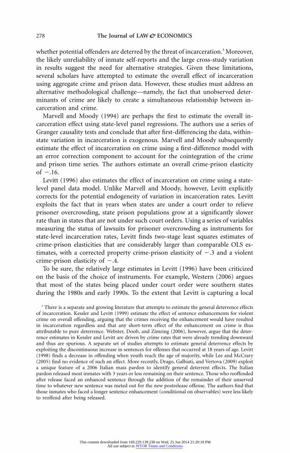
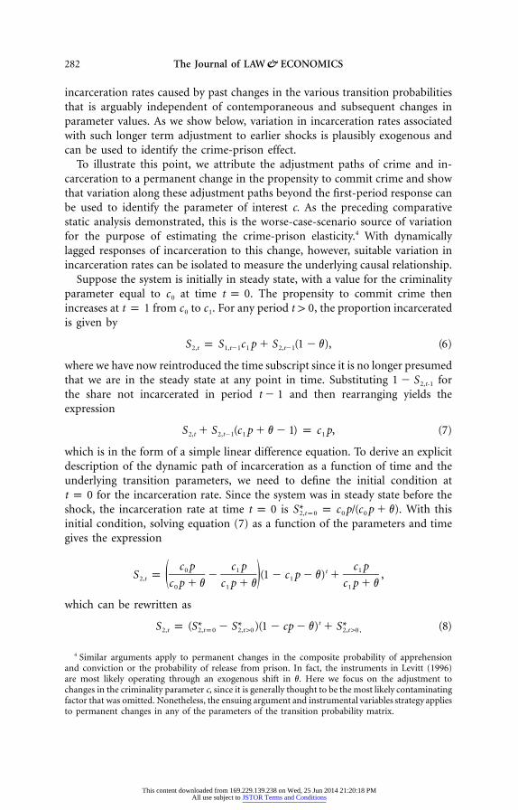
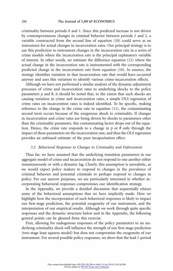
Figure 1. The dynamic adjustment path of incarceration and crime rates
where is the old steady-state incarceration rate prior toS* p c p/(c p � v)2,tp0 0 0
the change in criminality and is the new steady-state in-S* p c p/(c p � v)12,t 0 1 1
carceration rate that will eventually be reached given stability in the parametersand enough time.
Equation (8) shows that the incarceration rate at any time is equal tot 1 0the new steady-state incarceration rate (the second term on the right) plus aproportion of the disparity between the old and new steady-state rates. Sincethe first term is negative, and since for typical values of0 ! (1 � cp � v) ! 1these parameters,5 equation (8) depicts a stable process whereby the incarcerationrate approaches the new steady state from below. The adjustment path is depictedin Figure 1. Note that the incarceration rate increases between andt p 0 t p
because of the increase in the criminality parameter. Subsequent increases,1however, are not driven by further changes in c, since we have assumed a one-time permanent shock to criminality. Rather, subsequent increases reflect thedynamic multiperiod adjustment of incarceration toward its new equilibriumrate. For annual data for U.S. states, a typical value for v is roughly .5, while a
5 In theory, it is plausible that the term ( ) could fall below zero. This would require a1 � cp � vvery high release probability and a very large inflow rate into prison. If this were the case and if
, then the incarceration rate would still converge asymptotically to the higher�1 ! 1 � cp � v ! 0steady-state value. However, rather than approach the steady state from below, the adjustment pathwould oscillate above and below the long-run steady state, with the oscillation variance diminishingwith time. In practice, the prison release rate in the United States hovers around .5, and the transitioninto prison, cp, is consistently below .01. Hence, for practical purposes it is safe to assume that
.0 ! 1 � cp � v ! 1
This content downloaded from 169.229.139.238 on Wed, 25 Jun 2014 21:20:18 PMAll use subject to JSTOR Terms and Conditions
284 The Journal of LAW& ECONOMICS
typical value for cp (the flow rate into prison) is, at most, .01. These values,combined with equation (8), suggest that the incarceration rate becomes quiteclose to its new equilibrium value after 5 or 6 years.
We can derive a similar adjustment path for the crime rate. Substituting thetime path for incarceration into equation (5) and rearranging yields the ex-pression
tCrime p c (S* � S* )(1 � cp � v) � c (1 � S* ), (9)1 1t t 2,t 0 2,tp0 t 2,t 0
where the crime rate at time consists of two components: the new steady-t 1 0state crime rate (the second terms on the right-hand side of equation [9]), andthe deviation from the new steady state associated with the dynamics adjustment(the first term). Here the adjustment term is positive and approaches zero as tincreases, which implies that the crime rate approaches its new equilibrium fromabove. Given that the new steady-state crime rate will exceed the old steady-statecrime rate, equation (9) indicates that in response to a permanent increase incriminality, the crime rate increases discretely and then declines to the new equi-librium over time. The time path for this variable is also depicted in Figure 1.
The patterns observed in Figure 1 hint at our identification strategy. Betweenperiods and , both crime and incarceration rates increase as a resultt p 0 t p 1of the discrete increase in the criminality parameter from to . Clearly, thec c0 1
positive covariance between the two variables for this first difference (both crimeand incarceration rates increase) is driven by the change in criminality. Thus, aregression of a series of such first-period changes in the crime rate against afirst-period change in the incarceration rate will yield a spurious positive coef-ficient.
This is not the case, however, for subsequent changes in these series. For allchanges beyond the first, the criminality parameter is held constant, yet theincarceration rate increases as it approaches its new equilibrium rate. With regardto the crime rate, following the initial discrete increase, subsequent increases inthe incarceration rate decrease the crime rate by incapacitating a greater pro-portion of the population. In other words, the decline in the crime rate alongthe adjustment path beyond the change between periods 0 and 1 is driven bythe increase in the incarceration rate. In fact, the ratio of the changes in thecrime rate to the change in the incarceration rate for any of these subsequentperiods would yield �1 times the criminality parameter—that is, the incapac-itation effect that we seek to estimate. Thus, if one could discard the variationassociated with the initial shock and isolate variation in subsequent movementsassociated with the dynamics adjustment to the shock, one could identify theincapacitation effect of marginal increases in the incarceration rate.
The exogeneity of subsequent changes in the incarceration rate in this modelis best illustrated by deriving explicit expressions for the change in incarcerationand crime rates following permanent shocks to criminality. Let DS p2,t
and . From equation (8), explicit expressions for 1-S � S DC p C � C2,t�1 2,t t t�1 t
period changes in incarceration rates for , , and aret p 0 t p 1 t 1 1
This content downloaded from 169.229.139.238 on Wed, 25 Jun 2014 21:20:18 PMAll use subject to JSTOR Terms and Conditions
Crime Reduction 285
DS p (S* � S* )(c p � v),12,0 2,t 0 2,tp0 1
DS p (S* � S* )(c p � v)(1 � c p � v), (10)12,1 2,t 0 2,tp0 1 1
tDS p (S* � S* )(c p � v)(1 � c p � v) .12,t 2,t 0 2,tp0 1 1
Given that , the first change in the incarceration rate is the(1 � c p � v) ! 11
largest, and each subsequent change diminishes in size.By equation (9), an explicit expression for the first-period change in the crime
rate is
DCrime p �c DS � (c � c )(1 � S* ), (11)o 1 2,0 1 0 2,tp0
which has two components, one of which we are interested in uncovering. Thesecond term on the right-hand side of equation (11) gives the change in thecrime rate associated with the increase in criminality, holding the incarcerationrate at its equilibrium in period . This component is positive and drivest p 0the initial spike in crime rates. The first term on the right-hand side of equation(11) shows the association between the decline in crime rates and the first-periodincrease in incarceration rates. Thus, the discrete increase in crime rates in Figure1 entails the sum of two effects: the effect of an increase in criminality (the largerof the two) and the partially offsetting effect of the contemporaneous increasein incarceration.
In practice, we observe the total change in the crime rate and the change inthe incarceration rate, and we wish to estimate the coefficient associated�c1
with the first component in equation (11). We do not observe the second termon the right-hand side of equation (11), and thus it is swept into the residualof an OLS regression. Given that the contemporaneous change in criminalitywill be positively correlated with the contemporaneous change in the incarcer-ation rate, an OLS regression of on will yield a positively biasedDCrime DS0 2,0
estimate of . This argument is similar to the identification problem that we�c1
highlighted in the comparative static analysis.However, changes subsequent to the first-period change will not suffer from
this bias. To see this, the explicit expression for the next change in crime is givenby
DCrime p �c DS . (12)1 1 2,1
Here the crime rate change is a function of the change in incarceration ratesalone. This follows from the fact that we are modeling a one-time permanentincrease in criminality, and thus the contaminating second term in equation (11)drops out for all subsequent changes in crime rates until the crime rate reachesits new steady-state level. Most important, taking the ratio of equation (12) tothe second line of equation (10) yields the parameter of interest .�c1
Together, equations (10) and (12) provide the heart of our identificationstrategy. The second line of equation (10) provides a prediction for the changein incarceration rates between periods 1 and 2 associated with an increase in
This content downloaded from 169.229.139.238 on Wed, 25 Jun 2014 21:20:18 PMAll use subject to JSTOR Terms and Conditions
286 The Journal of LAW& ECONOMICS
criminality between periods 0 and 1. Since this predicted increase is not drivenby contemporaneous changes in criminal behavior between periods 1 and 2, avariable constructed from the second line of equation (10) could serve as aninstrument for actual changes in incarceration rates. Our principal strategy is touse this prediction to instrument changes in the incarceration rate in a series ofcrime models where the incarceration rate is the principal explanatory variableof interest. In other words, we estimate the difference equation (12) where theactual change in the incarceration rate is instrumented with the correspondingpredicted change in the incarceration rate from equation (10). In essence, thestrategy identifies variation in that incarceration rate that would have occurredanyway and uses this variation to identify various crime-incarceration effects.
Although we have not performed a similar analysis of the dynamic adjustmentprocesses of crime and incarceration rates to underlying shocks to the policyparameters p and v, it should be noted that, to the extent that such shocks arecausing variation in crime and incarceration rates, a simple OLS regression ofcrime rates on incarceration rates is indeed identified. To be specific, makingreference to the change in the crime rate in equation (11), the contaminatingsecond term occurs because of the exogenous shock to criminality. If changesin incarceration and crime rates are being driven by shocks to parameters otherthan the criminality parameter, this contaminating factor drops out of the equa-tion. Hence, the crime rate responds to a change in p or v only through theimpact of these parameters on the incarceration rate, and thus the OLS regressionprovides an unbiased estimate of the pure incapacitation effect.
3.2. Behavioral Responses to Changes in Criminality and Enforcement
Thus far, we have assumed that the underlying transition parameters in ouraggregate model of crime and incarceration do not respond to one another eitherinstantaneously or with a dynamic lag. Clearly, this assumption is unrealistic, aswe would expect policy makers to respond to changes in the prevalence ofcriminal behavior and potential criminals to perhaps respond to changes inpolicy. For our narrow purposes, we are particularly interested in whether in-corporating behavioral responses compromises our identification strategy.
In the Appendix, we provide a detailed discussion that sequentially relaxessome of the behavioral assumptions that we have implicitly made. Here wehighlight how the incorporation of such behavioral responses is likely to impactour first-stage prediction, the potential exogeneity of our instrument, and theinterpretation of our empirical results. Although we work through quite specificresponses and the dynamic structure below and in the Appendix, the followinggeneral points can be gleaned from this exercise.
First, allowing for endogenous responses of the policy parameters to an un-derlying criminality shock will influence the strength of our first-stage prediction(two-stage least squares model) but does not compromise the exogeneity of ourinstrument. For several possible policy responses, we show that the lead 1-period
This content downloaded from 169.229.139.238 on Wed, 25 Jun 2014 21:20:18 PMAll use subject to JSTOR Terms and Conditions
Crime Reduction 287
change in incarceration rates can be decomposed into a component equal toour prediction, assuming no behavioral response (via equation [10]) as well asadditional components associated with the second-order responsive changes inp and v. Since these parameters influence crime only through the incapacitationand deterrence effects of incarceration, we can still identify a causal effect aslong as our instrument predicts significant variation in the change in incarcer-ation rates.
Second, when we allow for a reciprocally responsive relationship betweencriminality and enforcement, we can no longer interpret the key coefficient asmeasuring a pure incapacitation effect (as in our simple model above). To bespecific, increases in enforcement caused by an exogenous shock to behaviormay induce any increase in criminality to be subsequently dulled by the higherincarceration risk. When this is the case, the empirical association between in-carceration and crime will be driven by incapacitation as well as deterrence. Inthe context of our instrumental variables strategy, our estimates will yield abiased estimate of the pure incapacitation effect. However, our estimate of thetotal effect of prison on crime is unbiased as long as we interpret the estimatemore broadly.
Finally, there are certain conditions under which the identification strategyproposed here would fail. The most obvious would be when changes in thecriminality parameter exhibit negative serial correlation for reasons that areindependent of policy. For example, if a wave of drug-related crime today leadsto the emergence of informal social controls that are external to the criminaljustice system that subsequently reduces criminality, the predicted future increasein incarceration rates may be spuriously inversely related to future decreases incrime rates.
In the Appendix, we provide a more detailed analysis of the consequences ofallowing for the following behavioral relationships.
Allowing Enforcement to Respond to Changes in Criminality: . Onep p p(c)might hypothesize that p may be either increasing or decreasing in the degreeof criminality. If policy makers increase enforcement in response to an increasein c, an elevated propensity to commit crime may be matched by an elevatedincarceration risk. On the other hand, an increase in c may dilute enforcementresources and reduce the risk of incarceration. Such a policy reaction shouldnot compromise the exogeneity of our instrument, although the timing of theresponse may impact the strength of our first-stage prediction. If p responds tochanges in c instantaneously, the behavioral response will either speed up orslow down the adjustment processes of crime and incarceration rates to theirnew equilibrium values (depending on the sign of dp/dc). If p responds with alag, our instrument will either overpredict or underpredict the actual change inincarceration rates. However, the proposed instrument is still orthogonal to thesecond-stage error term.
Allowing Sentence Severity to Respond to Changes in Criminality: . As-v p v(c)sessing the effect of a change in sentence length on our identification strategy
This content downloaded from 169.229.139.238 on Wed, 25 Jun 2014 21:20:18 PMAll use subject to JSTOR Terms and Conditions
288 The Journal of LAW& ECONOMICS
by necessity requires a dynamic analysis, since a change in sentence length todaywill not impact incarceration rates until today’s cohort of admitted inmates reachtheir counterfactual release dates under the prior sentencing regime. Assuminga 1-period lag in the response of v to a change in c, an increase in sentencelength (operationalized as a decrease in v) in response to an increase in c impliesthat our instrument will underpredict the change in incarceration rates after theinitial behavioral shock. Although this introduces error into our first-stage pre-diction, the instrument is still exogenous to the unobserved determinants offuture changes in crime rates.
Allowing Criminality and Enforcement to React Reciprocally: p p p(c), c p. The implications of allowing simultaneous determination of the crimi-c(p)
nality and incarceration risk parameters for our identification strategy will dependon whether these adjustments will occur instantaneously or over time. Moreover,if the reaction processes are dynamic, the timing and sequencing of the reactionsare important in assessing how such behavioral responses would impact theinterpretation of our empirical results. If we assume that criminality respondsto changes in p instantaneously, while enforcement responds to changes in cwith a lag, our proposed instrumental variables strategy will yield a biased es-timate of a pure incapacitation effect. This bias is driven by the fact that theerror term in the second-stage equation relating changes in crime rates to changesin incarceration rates will include a component reflecting the behavioral responseof criminal behavior to enhanced enforcement (a term that will be negativelycorrelated with our predicted change in incarceration). However, since this com-ponent is essentially a general deterrent effect, the structural estimate of the effectof incarceration on crime still represents a causal effect, as long as this estimateis interpreted as the overall impact of a change in incarceration rates (incapac-itation plus deterrence). With regard to the first-stage prediction, reciprocalreactionary responses between p and c imply that future increases in incarcerationrates in response to a change in c may be either smaller or larger than a non-behavioral model would predict, since the effect of enhanced enforcement onincarceration rates is offset by subsequent deterrence-induced declines incriminality.
Allowing Future Change in Criminality to Respond to a Previous Change inCriminality. Suppose that current increases in criminal behavior cause subse-quent decreases in criminality because of a revulsion on the part of those likelyto commit crime in response to the consequences of an initial crime spike. Suchan effect would induce negative serial correlation in changes in the criminalityparameter and would likely induce a spurious negative correlation between ourinstrument (which is increasing in the past period’s increase in criminality be-havior) and future changes in crime rates (which would be negatively impactedby the hypothesized reactive behavior). Of course, if the periodicity of our datais such that the 1-period lead prediction we employ as an instrument predictschanges in incarceration before such revulsion wells up and impacts crime, ourIV strategy would still be valid.
This content downloaded from 169.229.139.238 on Wed, 25 Jun 2014 21:20:18 PMAll use subject to JSTOR Terms and Conditions
Crime Reduction 289
To summarize, with the exception of the final possibility, incorporating be-havior into our model may impact the precision of our first-stage predictionbut does not compromise the exogeneity of the proposed instrument. If we allowcriminal behavior and corrections policy to respond simultaneously to one an-other, we need to interpret the IV results as an overall effect of incarceration oncrime rather than as an estimate of a pure incapacitation effect. Nonetheless,the IV estimates still carry a causal interpretation.
Our strategy would not be suitable if criminal behavior reacts negatively toprevious increases in criminal behavior (through channels not mediated by achange in enforcement or sentencing). Above we offer the example of the emer-gence of informal social controls intended to mitigate an increase in criminality.However, there are strong reasons to believe that such responses would likelytake more than 1 year (the time frame of our prediction) and thus are unlikelyto compromise our results. Nonetheless, we acknowledge this potential weakness.
3.3. Heterogeneity in the Propensity to Commit Crime
In our theoretical model, we made the simplifying assumption that the crim-inality parameter c was constant across the population. This assumption thuspermits identification of a constant incapacitation effect. To be sure, this pa-rameter most likely has a nondegenerate distribution among the general public,and the conditional expectation of c among the incarcerated (as well the valueon the margin for recent prison entrant) likely depends on the overall incar-ceration rate (with all else held equal, one would expect lower average values ofc among inmates the higher the incarceration rate). With heterogeneity in thecriminality parameter, estimates of the joint incapacitation/deterrence effectsshould be interpreted as local average treatment effects specific to the periodcovered by the underlying data. One of the key motivations driving this analysisis to test for such heterogeneity, specifically with regard to alternative periodswith different average incarceration rates.
4. Data Description and Documentation of the First-Stage Relationship
Implementing our identification strategy requires that we obtain informationon the transition probabilities between incarceration and nonincarceration bystate and year. Our strategy also requires that we identify permanent changes inunderlying transition probabilities. Finally, there are very few states and periodsin which changes in incarceration rates fit the model of a one-time increase incriminality with a delayed dynamic adjustment. In fact, over the past 20 or moreyears, most states have experienced repeated increases in prison admission rates.Thus, we must adapt our strategy to incorporate these serial shocks. Here wedescribe the data for this project and the manner in which we use these data toimplement our identification strategy.
Our first task is to estimate the transition probabilities by state and year, since
This content downloaded from 169.229.139.238 on Wed, 25 Jun 2014 21:20:18 PMAll use subject to JSTOR Terms and Conditions
290 The Journal of LAW& ECONOMICS
Table 1
Illustration of the Calculation of the Predicted Change inIncarceration Rates for New York, 1979–82
1979 1980 1981 1982
Current incarceration rate ( )S2,t 118.39 125.33 147.30 161.39Admission rate (cp) .00059 .00071 .00072Release rate (v) .432 .329 .360Equilibrium incarceration rate based
on current transition probabilities( )S* p [cp/(cp � v)] # 100,00012,t 0 135.87 215.61 199.97
Incarceration rate at t p 0 ( )S2,0 118.39 125.33 147.30Predicted change in incarceration ratea
[ ](S* � S ) # (1 � cp � v)(cp � v)12,t 0 2,0 4.29 19.94 12.15Actual change in incarceration ratea 21.97 14.09 13.64
a From t p 1 to t p 2.
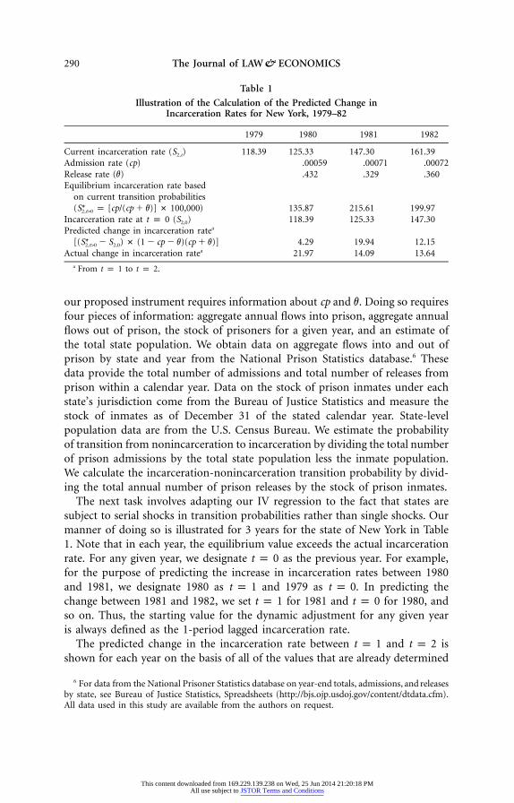
our proposed instrument requires information about cp and v. Doing so requiresfour pieces of information: aggregate annual flows into prison, aggregate annualflows out of prison, the stock of prisoners for a given year, and an estimate ofthe total state population. We obtain data on aggregate flows into and out ofprison by state and year from the National Prison Statistics database.6 Thesedata provide the total number of admissions and total number of releases fromprison within a calendar year. Data on the stock of prison inmates under eachstate’s jurisdiction come from the Bureau of Justice Statistics and measure thestock of inmates as of December 31 of the stated calendar year. State-levelpopulation data are from the U.S. Census Bureau. We estimate the probabilityof transition from nonincarceration to incarceration by dividing the total numberof prison admissions by the total state population less the inmate population.We calculate the incarceration-nonincarceration transition probability by divid-ing the total annual number of prison releases by the stock of prison inmates.
The next task involves adapting our IV regression to the fact that states aresubject to serial shocks in transition probabilities rather than single shocks. Ourmanner of doing so is illustrated for 3 years for the state of New York in Table1. Note that in each year, the equilibrium value exceeds the actual incarcerationrate. For any given year, we designate as the previous year. For example,t p 0for the purpose of predicting the increase in incarceration rates between 1980and 1981, we designate 1980 as and 1979 as . In predicting thet p 1 t p 0change between 1981 and 1982, we set for 1981 and for 1980, andt p 1 t p 0so on. Thus, the starting value for the dynamic adjustment for any given yearis always defined as the 1-period lagged incarceration rate.
The predicted change in the incarceration rate between and ist p 1 t p 2shown for each year on the basis of all of the values that are already determined
6 For data from the National Prisoner Statistics database on year-end totals, admissions, and releasesby state, see Bureau of Justice Statistics, Spreadsheets (http://bjs.ojp.usdoj.gov/content/dtdata.cfm).All data used in this study are available from the authors on request.
This content downloaded from 169.229.139.238 on Wed, 25 Jun 2014 21:20:18 PMAll use subject to JSTOR Terms and Conditions
Crime Reduction 291
by time period (with the exception of the initial incarceration rate, whicht p 1is determined by ), using the second expression in equation (10). Actualt p 0change in incarceration rates between and is calculated by usingt p 1 t p 2the predicted change in incarceration rates as an instrument for the first differ-ences in incarceration rates.
Finally, our identification strategy requires that we identify permanent changesto the underlying transition probabilities (which may subsequently be enhancedor diminished by future changes in these probabilities). To the extent that theobserved changes in empirical admission and release hazards reflect temporaryrather than permanent changes, our instrument will serve as a poor predictorof future actual change in incarceration rates.7 To minimize the influence oftemporary shocks to the transition probabilities, we first smooth the transitionprobability time series for each state and use the smoothed series to constructthe predicted change in incarceration rates as illustrated in Table 1. For eachstate, we estimate a simple regression where a given transition probability isregressed on an eighth-order polynomial time trend. We then calculate the pre-dicted value for the transition probability from the estimated regression function.We estimate this model for each of the 50 states plus Washington, D.C., for theadmission hazard as well as the release hazard (102 models in all). These predictedtransition probabilities are then used to construct our instrumental variable.8
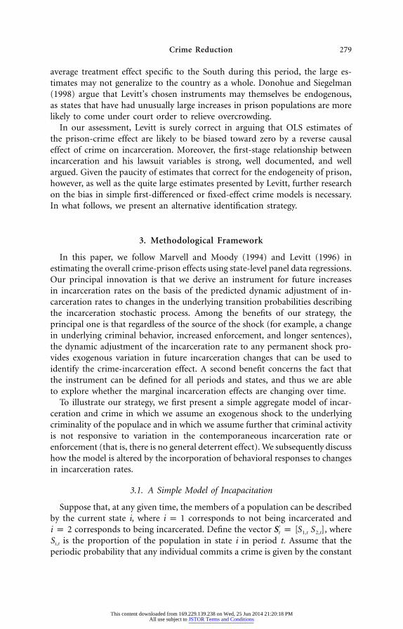
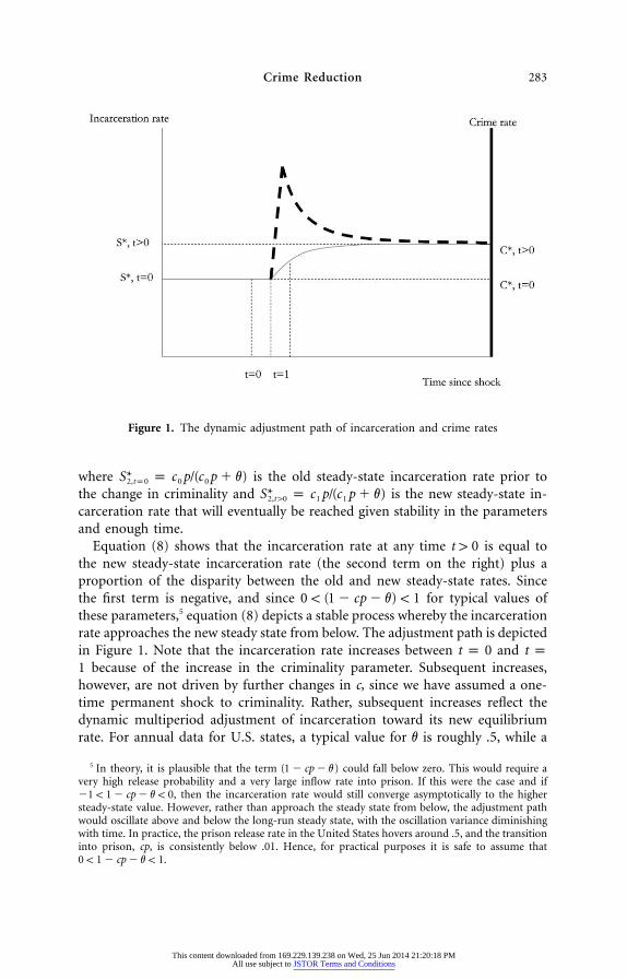
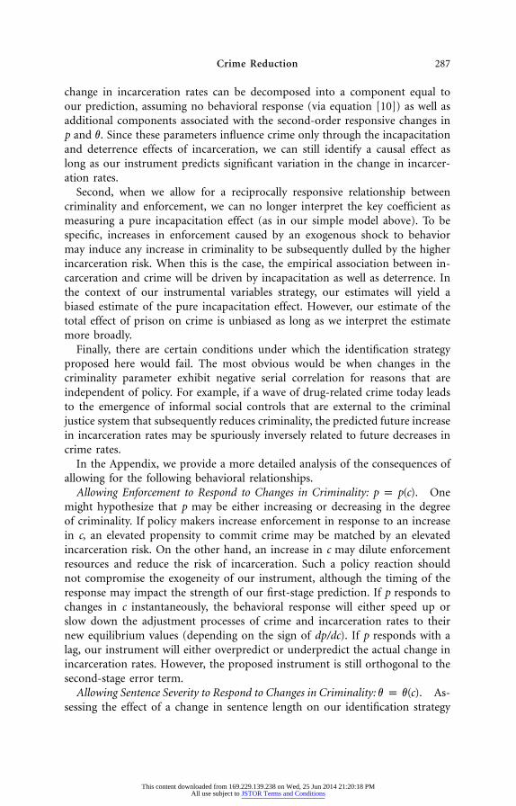
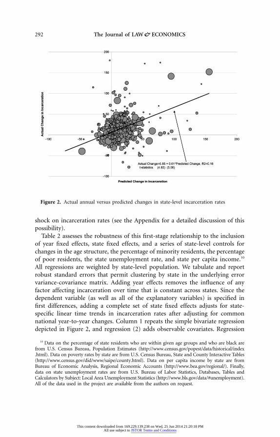
Our panel data set covers the period 1978–2004 and the 50 states and Wash-ington, D.C.9 Figure 2 presents a simple bivariate scatterplot (weighted by state-level population counts) of the actual annual changes in incarceration rates forthe entire panel against the predicted changes from equation (10) (using thesmoothed state-level transition probabilities). Several notable patterns stand out.First, there is a strong correlation between our instrument and actual changesin incarceration rates (approximately .40), with the instrument explainingroughly 16 percent of the variation in annual changes. Second, the lion’s shareof predicted increases in incarceration are positive (approximately 86 percent),which suggests that for most states and periods, the observed incarceration rateis below the steady-state rate implied by the value of their transition probabilities.Finally, the coefficient on the instrument is substantially less than 1 (.61), whichsuggests that the instrument is overpredicting the actual change in incarcerationrates. Note that this is consistent with a reciprocal responsiveness between crim-inal propensity and enforcement, with subsequent declines in criminality oc-curring in response to enhanced enforcement moderating the impact of a crime
7 Moreover, if temporary increases in criminality cause subsequent increases in incarceration ratesbecause of time lags between arrest and incarceration or a spurt of criminal activity at the end ofthe year, temporary shocks to the transition probabilities may induce a spurious negative relationshipbetween our instrument and crime.
8 In the remainder of Section 4, we discuss results that use the unsmoothed parameter values toconstruct the instrument as well.
9 There are a few missing observations for Alaska and two missing observations at the end of thetime series for Washington, D.C., when the metropolitan area abandoned its prison system.
This content downloaded from 169.229.139.238 on Wed, 25 Jun 2014 21:20:18 PMAll use subject to JSTOR Terms and Conditions
292 The Journal of LAW& ECONOMICS
Figure 2. Actual annual versus predicted changes in state-level incarceration rates
shock on incarceration rates (see the Appendix for a detailed discussion of thispossibility).
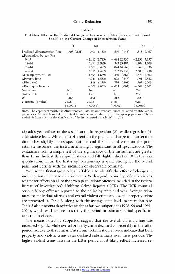
Table 2 assesses the robustness of this first-stage relationship to the inclusionof year fixed effects, state fixed effects, and a series of state-level controls forchanges in the age structure, the percentage of minority residents, the percentageof poor residents, the state unemployment rate, and state per capita income.10
All regressions are weighted by state-level population. We tabulate and reportrobust standard errors that permit clustering by state in the underlying errorvariance-covariance matrix. Adding year effects removes the influence of anyfactor affecting incarceration over time that is constant across states. Since thedependent variable (as well as all of the explanatory variables) is specified infirst differences, adding a complete set of state fixed effects adjusts for state-specific linear time trends in incarceration rates after adjusting for commonnational year-to-year changes. Column 1 repeats the simple bivariate regressiondepicted in Figure 2, and regression (2) adds observable covariates. Regression
10 Data on the percentage of state residents who are within given age groups and who are black arefrom U.S. Census Bureau, Population Estimates (http://www.census.gov/popest/data/historical/index.html). Data on poverty rates by state are from U.S. Census Bureau, State and County Interactive Tables(http://www.census.gov/did/www/saipe/county.html). Data on per capita income by state are fromBureau of Economic Analysis, Regional Economic Accounts (http://www.bea.gov/regional/). Finally,data on state unemployment rates are from U.S. Bureau of Labor Statistics, Databases, Tables andCalculators by Subject: Local Area Unemployment Statistics (http://www.bls.gov/data/#unemployment).All of the data used in the project are available from the authors on request.
This content downloaded from 169.229.139.238 on Wed, 25 Jun 2014 21:20:18 PMAll use subject to JSTOR Terms and Conditions
Crime Reduction 293
Table 2
First-Stage Effect of the Predicted Change in Incarceration Rates (Based on Last-PeriodShock) on the Current Change in Incarceration Rates
(1) (2) (3) (4)
Predicted DIncarceration Rate .605 (.121) .603 (.133) .549 (.143) .513 (.167)DPopulation, by age (%):
0–17 �2.415 (2.715) �.684 (2.530) �2.236 (3.057)18–24 �3.871 (4.989) .393 (3.483) �1.109 (4.009)25–44 �2.602 (3.492) �1.074 (4.565) �1.968 (5.236)45–64 �3.619 (4.472) 1.752 (5.137) 2.386 (5.438)
DUnemployment Rate �1.595 (.659) �1.430 (.861) �1.378 (.902)DPoverty Rate �.943 (.532) .078 (.547) .091 (.552)DBlack (%) .819 (.135) .736 (.203) .793 (.203)DPer Capita Income �.008 (.002) �.005 (.002) �.004 (.002)Year effects No No Yes YesState effects No No No YesR2 .164 .190 .312 .328F-statistic (p value) 24.96 20.63 14.83 9.45
(!.0001) (!.0001) (!.0003) (!.0035)
Note. The dependent variable is DIncarceration Rate. Robust standard errors, clustered by state, are inparentheses. All models include a constant terms and are weighted by the state-year populations. The F-statistic is from a test of the significance of the instrumental variable. N p 1,321.
(3) adds year effects to the specification in regression (2), while regression (4)adds state effects. While the coefficient on the predicted change in incarcerationdiminishes slightly across specifications and the standard error on the pointestimate increases, the instrument is highly significant in all specifications. TheF-statistics from a simple test of the significance of the instrument are greaterthan 10 in the first three specifications and fall slightly short of 10 in the finalspecification. Thus, the first-stage relationship is quite strong for the overallpanel and persists with the inclusion of observable covariates.
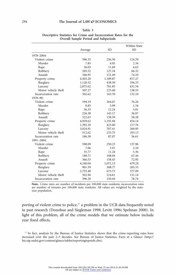
We use the first-stage models in Table 2 to identify the effect of changes inincarceration on changes in crime rates. With regard to our dependent variables,we test for effects on all of the seven part I felony offenses included in the FederalBureau of Investigation’s Uniform Crime Reports (UCR). The UCR count allserious felony offenses reported to the police by state and year. Average crimerates for individual offenses and overall violent crime and overall property crimeare presented in Table 3, along with the average state-level incarceration rate.Table 3 also presents descriptive statistics for two subperiods (1978–90 and 1991–2004), which we later use to stratify the period to estimate period-specific in-carceration effects.
The means noted by subperiod suggest that the overall violent crime rateincreased slightly, while overall property crime declined considerably in the latterperiod relative to the former. Data from victimization surveys indicate that bothproperty and violent crime rates declined substantially over these periods. Thehigher violent crime rates in the latter period most likely reflect increased re-
This content downloaded from 169.229.139.238 on Wed, 25 Jun 2014 21:20:18 PMAll use subject to JSTOR Terms and Conditions
294 The Journal of LAW& ECONOMICS
Table 3
Descriptive Statistics for Crime and Incarceration Rates for theOverall Sample Period and Subperiods
Average SDWithin-State
SD
1978–2004:Violent crime 596.35 256.50 124.70
Murder 7.85 4.05 2.34Rape 36.03 11.69 6.63Robbery 205.52 127.34 66.32Assault 346.95 151.49 74.10
Property crime 4,503.20 1,189.87 817.27Burglary 1,120.32 438.50 356.33Larceny 2,875.62 701.85 431.54Motor vehicle theft 507.27 223.40 138.55
Incarceration rate 302.62 163.70 132.101978–90:
Violent crime 594.19 264.07 76.26Murder 8.85 3.99 1.54Rape 36.33 12.24 5.01Robbery 226.38 145.17 36.07Assault 322.63 138.59 58.28
Property crime 4,929.62 1,191.04 454.14Burglary 1,392.10 423.60 217.76Larceny 3,024.91 707.41 260.95Motor vehicle theft 512.62 233.75 103.13
Incarceration rate 186.38 87.07 56.611991–2004:
Violent crime 598.09 250.23 137.96Murder 7.06 3.91 2.10Rape 35.77 11.24 5.36Robbery 188.71 108.04 67.44Assault 366.53 158.43 72.95
Property crime 4,160.04 1,072.13 679.24Burglary 901.59 308.77 205.33Larceny 2,755.48 673.73 377.09Motor vehicle theft 502.96 214.61 131.14
Incarceration rate 396.20 150.44 78.74
Note. Crime rates are number of incidents per 100,000 state residents; incarceration ratesare number of inmates per 100,000 state residents. All values are weighted by the state-year population.
porting of violent crime to police,11 a problem in the UCR data frequently notedin past research (Donohue and Siegleman 1998; Levitt 1996; Spelman 2000). Inlight of this problem, all of the crime models that we estimate below includeyear fixed effects.
11 In fact, analysis by the Bureau of Justice Statistics shows that the crime-reporting rates haveincreased over the past 2–3 decades. See Bureau of Justice Statistics, Facts at a Glance (http://bjs.ojp.usdoj.gov/content/glance/tables/reportingtypetab.cfm).
This content downloaded from 169.229.139.238 on Wed, 25 Jun 2014 21:20:18 PMAll use subject to JSTOR Terms and Conditions
Crime Reduction 295
5. Empirical Results Using the Entire Sample Period
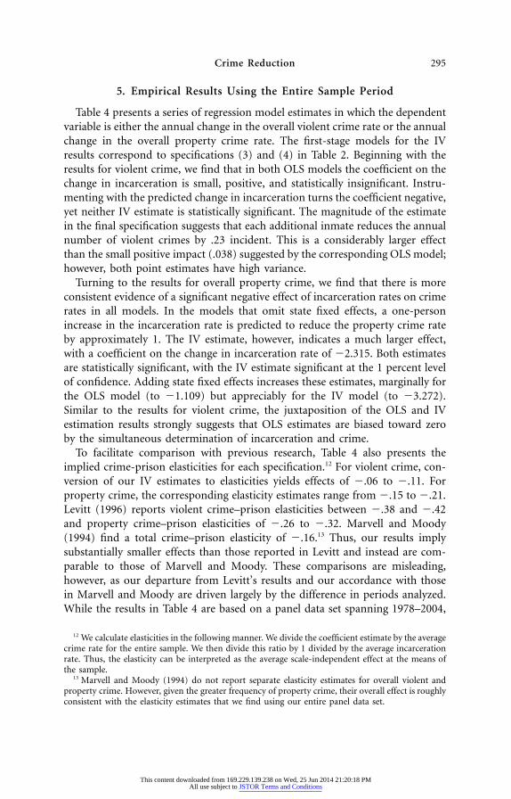
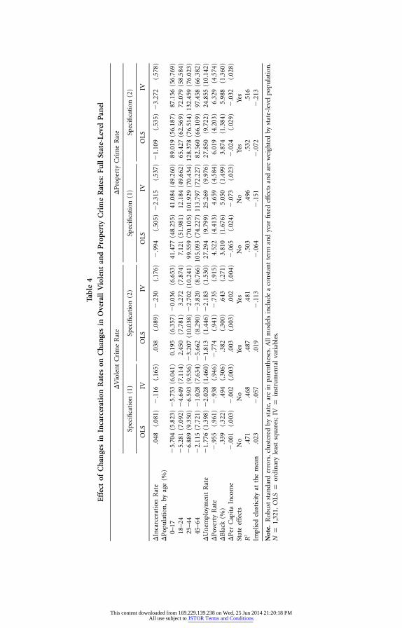
Table 4 presents a series of regression model estimates in which the dependentvariable is either the annual change in the overall violent crime rate or the annualchange in the overall property crime rate. The first-stage models for the IVresults correspond to specifications (3) and (4) in Table 2. Beginning with theresults for violent crime, we find that in both OLS models the coefficient on thechange in incarceration is small, positive, and statistically insignificant. Instru-menting with the predicted change in incarceration turns the coefficient negative,yet neither IV estimate is statistically significant. The magnitude of the estimatein the final specification suggests that each additional inmate reduces the annualnumber of violent crimes by .23 incident. This is a considerably larger effectthan the small positive impact (.038) suggested by the corresponding OLS model;however, both point estimates have high variance.
Turning to the results for overall property crime, we find that there is moreconsistent evidence of a significant negative effect of incarceration rates on crimerates in all models. In the models that omit state fixed effects, a one-personincrease in the incarceration rate is predicted to reduce the property crime rateby approximately 1. The IV estimate, however, indicates a much larger effect,with a coefficient on the change in incarceration rate of �2.315. Both estimatesare statistically significant, with the IV estimate significant at the 1 percent levelof confidence. Adding state fixed effects increases these estimates, marginally forthe OLS model (to �1.109) but appreciably for the IV model (to �3.272).Similar to the results for violent crime, the juxtaposition of the OLS and IVestimation results strongly suggests that OLS estimates are biased toward zeroby the simultaneous determination of incarceration and crime.
To facilitate comparison with previous research, Table 4 also presents theimplied crime-prison elasticities for each specification.12 For violent crime, con-version of our IV estimates to elasticities yields effects of �.06 to �.11. Forproperty crime, the corresponding elasticity estimates range from �.15 to �.21.Levitt (1996) reports violent crime–prison elasticities between �.38 and �.42and property crime–prison elasticities of �.26 to �.32. Marvell and Moody(1994) find a total crime–prison elasticity of �.16.13 Thus, our results implysubstantially smaller effects than those reported in Levitt and instead are com-parable to those of Marvell and Moody. These comparisons are misleading,however, as our departure from Levitt’s results and our accordance with thosein Marvell and Moody are driven largely by the difference in periods analyzed.While the results in Table 4 are based on a panel data set spanning 1978–2004,
12 We calculate elasticities in the following manner. We divide the coefficient estimate by the averagecrime rate for the entire sample. We then divide this ratio by 1 divided by the average incarcerationrate. Thus, the elasticity can be interpreted as the average scale-independent effect at the means ofthe sample.
13 Marvell and Moody (1994) do not report separate elasticity estimates for overall violent andproperty crime. However, given the greater frequency of property crime, their overall effect is roughlyconsistent with the elasticity estimates that we find using our entire panel data set.
This content downloaded from 169.229.139.238 on Wed, 25 Jun 2014 21:20:18 PMAll use subject to JSTOR Terms and Conditions
Tabl
e4
Eff
ect
ofC
han
ges
inIn
carc
erat
ion
Rat
eson
Cha
nge
sin
Ove
rall
Vio
len
tan
dP
rope
rty
Cri
me
Rat
es:
Full
Stat
e-Le
vel
Pan
el
DV
iole
nt
Cri
me
Rat
eD
Pro
pert
yC
rim
eR
ate
Spec
ifica
tion
(1)
Spec
ifica
tion
(2)
Spec
ifica
tion
(1)
Spec
ifica
tion
(2)
OL
SIV
OL
SIV
OL
SIV
OL
SIV
DIn
carc
erat
ion
Rat
e.0
48(.
081)
�.1
16(.
165)
.038
(.08
9)�
.230
(.17
6)�
.994
(.50
5)�
2.31
5(.
537)
�1.
109
(.53
5)�
3.27
2(.
578)
DP
opu
lati
on,
byag
e(%
)0–
17�
5.70
4(5
.823
)�
5.75
3(6
.041
)0.
195
(6.3
57)
�0.
036
(6.6
53)
41.4
77(4
8.25
5)41
.084
(49.
260)
89.0
19(5
6.18
7)87
.156
(56.
769)
18–2
4�
5.28
1(7
.092
)�
4.64
9(7
.114
)2.
450
(7.7
81)
3.27
2(7
.874
)7.
121
(51.
981)
12.1
84(4
9.66
2)65
.427
(62.
569)
72.0
79(5
8.58
4)25
–44
�6.
889
(9.3
50)
�6.
593
(9.5
36)
�3.
207
(10.
038)
�2.
702
(10.
241)
99.5
59(7
0.10
5)10
1.92
9(7
0.43
4)12
8.37
8(7
6.51
4)13
2.45
9(7
6.02
3)45
–64
�2.
115
(7.7
21)
�1.
028
(7.6
34)
�5.
662
(8.2
90)
�3.
820
(8.7
66)
105.
093
(74.
227)
113.
797
(72.
227)
82.5
60(6
6.10
9)97
.458
(66.
382)
DU
nem
ploy
men
tR
ate
�1.
776
(1.3
98)
�2.
028
(1.4
60)
�1.
813
(1.4
46)
�2.
183
(1.5
30)
27.2
94(9
.799
)25
.269
(9.9
76)
27.8
50(9
.722
)24
.855
(10.
142)
DP
over
tyR
ate
�.9
55(.
961)
�.9
38(.
946)
�.7
74(.
941)
�.7
35(.
915)
4.52
2(4
.413
)4.
659
(4.5
84)
6.01
9(4
.203
)6.
329
(4.5
74)
DB
lack
(%)
.339
(.32
2).4
94(.
306)
.382
(.30
0).6
43(.
271)
3.81
0(1
.676
)5.
050
(1.4
99)
3.87
4(1
.384
)5.
988
(1.3
60)
DP
erC
apit
aIn
com
e�
.001
(.00
3)�
.002
(.00
3).0
03(.
003)
.002
(.00
4)�
.065
(.02
4)�
.073
(.02
3)�
.024
(.02
9)�
.032
(.02
8)St
ate
effe
cts
No
No
Yes
Yes
No
No
Yes
Yes
R2
.471
.468
.487
.481
.503
.496
.532
.516
Impl
ied
elas
tici
tyat
the
mea
n.0
23�
.057
.019
�.1
13�
.064
�.1
51�
.072
�.2
13
Not
e.R
obu
stst
anda
rder
rors
,cl
ust
ered
byst
ate,
are
inpa
ren
thes
es.
All
mod
els
incl
ude
aco
nst
ant
term
and
year
fixe
def
fect
san
dar
ew
eigh
ted
byst
ate-
leve
lpop
ula
tion
.N
p1,
321.
OLS
por
din
ary
leas
tsq
uar
es;
IVp
inst
rum
enta
lva
riab
les.
This content downloaded from 169.229.139.238 on Wed, 25 Jun 2014 21:20:18 PMAll use subject to JSTOR Terms and Conditions
Crime Reduction 297
Table 5
Effect of Changes in Incarceration Rates on Changes in IndividualCrimes: Full State-Level Panel
Specification (1) Specification (2)
Dependent Variable OLS IV OLS IV
DMurder �.002 (.002) �.005 (.006) �.001 (.002) �.005 (.006)DRape �.005 (.004) �.029 (.011) �.005 (.004) �.033 (.015)DRobbery �.025 (.035) �.165 (.111) �.028 (.035) �.227 (.136)DAssault .079 (.055) .082 (.163) .072 (.060) .035 (.192)DBurlgary �.398 (.124) �.857 (.273) �.414 (.129) �1.064 (.394)DLarceny �.498 (.286) �1.182 (.353) �.573 (.308) �1.720 (.296)DMotor vehicle theft �.097 (.137) �.275 (.253) �.122 (.138) �.487 (.274)Year effects Yes Yes Yes YesState effects No Yes No Yes
Note. Robust standard errors, clustered by state, are in parentheses. All models include a constant termand control variables for changes in the age structure, the percentage of minority residents, the percentageof poor residents, the state unemployment rate, and state per capita income. All models include year fixedeffects and are also weighted by state-level population. OLS p ordinary least squares; IV p instrumentalvariables.
Levitt’s analysis is based on panel data spanning 1971–93, and Marvell andMoody analyze the period 1971–89. As we show below, we find considerablylarger effects when we restrict our sample to an earlier time period. Moreover,unlike Marvell and Moody, we consistently find strong evidence that the crime-prison elasticities estimated by OLS are severely biased toward zero.
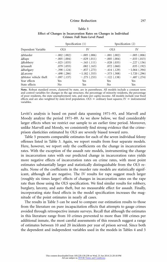
Table 5 presents comparable estimates for each of the seven individual felonyoffenses listed in Table 3. Again, we report results from four separate models.Here, however, we report only the coefficients on the change in incarcerationrates. With the exception of the assault rate models, instrumenting the changein incarceration rates with our predicted change in incarceration rates yieldsmore negative effects of incarceration rates on crime rates, with most pointestimates substantially larger and statistically distinguishable from the OLS re-sults. None of the coefficients in the murder rate models are statistically signif-icant, although all are negative. The IV results for rape suggest much larger(roughly six times larger) effects of changes in incarceration rates on the raperate than those using the OLS specification. We find similar results for robbery,burglary, larceny, and auto theft, but no measurable effect for assault. Finally,incorporating state fixed effects in the model specification increases the mag-nitude of the point estimates in nearly all cases.
The results in Table 5 can be used to compare our estimation results to thosefrom the literature on pure incapacitation effects that attempts to gauge crimesavoided through retrospective inmate surveys. Recall that although the estimatesin this literature range from 10 crimes prevented to more than 100 crimes peradditional inmate, the most careful assessments of this research suggest a rangeof estimates between 10 and 20 incidents per year of prison served. Since boththe dependent and independent variables used in the models in Tables 4 and 5
This content downloaded from 169.229.139.238 on Wed, 25 Jun 2014 21:20:18 PMAll use subject to JSTOR Terms and Conditions
298 The Journal of LAW& ECONOMICS
are expressed per 100,000 state residents, the coefficients on the change in theincarceration rate can be interpreted as the average effect of putting one moreperson in prison for a year. Thus, summing the coefficients for the seven crimecategories in Table 5 provides an estimate of the number of part I felony offensesprevented by putting one more person in prison.
One problem with this estimate concerns the fact that the UCR data are basedon crimes reported to the police, and with the exception of murder, reportingrates are considerably lower than 1 for all crimes. However, with crime-specificdata on reporting rates, one can easily inflate the point estimates by dividing bythe proportion of incidents reported to the police.
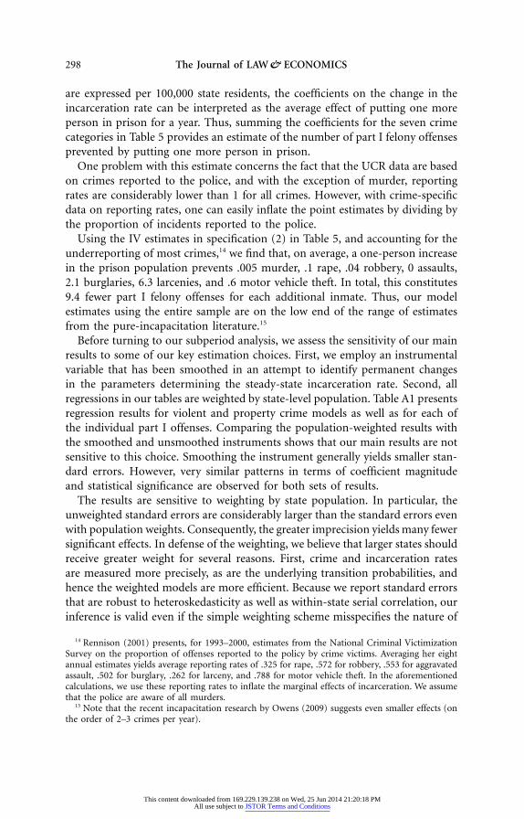
Using the IV estimates in specification (2) in Table 5, and accounting for theunderreporting of most crimes,14 we find that, on average, a one-person increasein the prison population prevents .005 murder, .1 rape, .04 robbery, 0 assaults,2.1 burglaries, 6.3 larcenies, and .6 motor vehicle theft. In total, this constitutes9.4 fewer part I felony offenses for each additional inmate. Thus, our modelestimates using the entire sample are on the low end of the range of estimatesfrom the pure-incapacitation literature.15
Before turning to our subperiod analysis, we assess the sensitivity of our mainresults to some of our key estimation choices. First, we employ an instrumentalvariable that has been smoothed in an attempt to identify permanent changesin the parameters determining the steady-state incarceration rate. Second, allregressions in our tables are weighted by state-level population. Table A1 presentsregression results for violent and property crime models as well as for each ofthe individual part I offenses. Comparing the population-weighted results withthe smoothed and unsmoothed instruments shows that our main results are notsensitive to this choice. Smoothing the instrument generally yields smaller stan-dard errors. However, very similar patterns in terms of coefficient magnitudeand statistical significance are observed for both sets of results.
The results are sensitive to weighting by state population. In particular, theunweighted standard errors are considerably larger than the standard errors evenwith population weights. Consequently, the greater imprecision yields many fewersignificant effects. In defense of the weighting, we believe that larger states shouldreceive greater weight for several reasons. First, crime and incarceration ratesare measured more precisely, as are the underlying transition probabilities, andhence the weighted models are more efficient. Because we report standard errorsthat are robust to heteroskedasticity as well as within-state serial correlation, ourinference is valid even if the simple weighting scheme misspecifies the nature of
14 Rennison (2001) presents, for 1993–2000, estimates from the National Criminal VictimizationSurvey on the proportion of offenses reported to the policy by crime victims. Averaging her eightannual estimates yields average reporting rates of .325 for rape, .572 for robbery, .553 for aggravatedassault, .502 for burglary, .262 for larceny, and .788 for motor vehicle theft. In the aforementionedcalculations, we use these reporting rates to inflate the marginal effects of incarceration. We assumethat the police are aware of all murders.
15 Note that the recent incapacitation research by Owens (2009) suggests even smaller effects (onthe order of 2–3 crimes per year).
This content downloaded from 169.229.139.238 on Wed, 25 Jun 2014 21:20:18 PMAll use subject to JSTOR Terms and Conditions
Crime Reduction 299
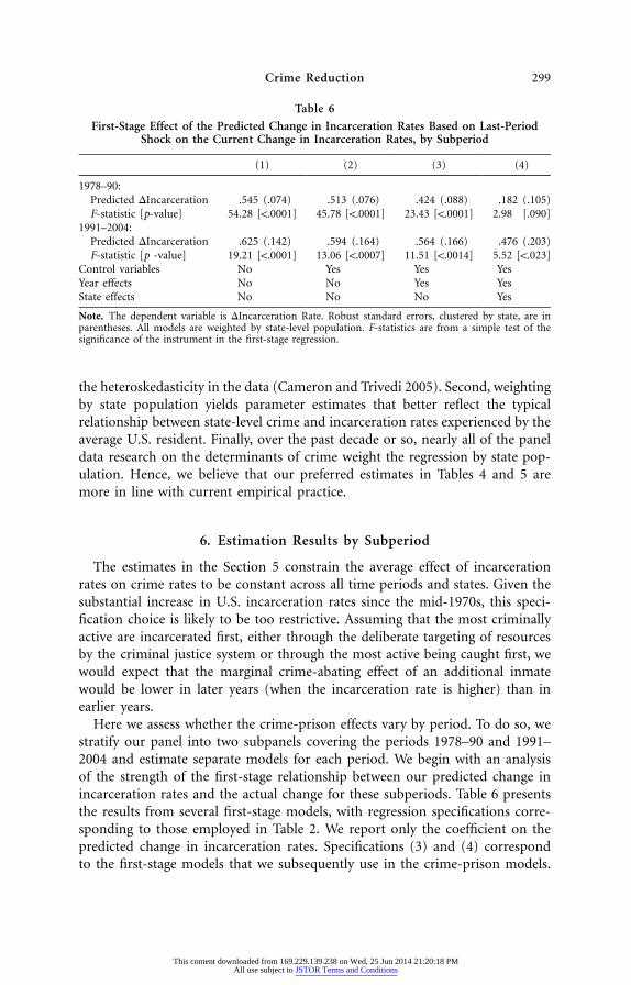
Table 6
First-Stage Effect of the Predicted Change in Incarceration Rates Based on Last-PeriodShock on the Current Change in Incarceration Rates, by Subperiod
(1) (2) (3) (4)
1978–90:Predicted DIncarceration .545 (.074) .513 (.076) .424 (.088) .182 (.105)F-statistic [p-value] 54.28 [!.0001] 45.78 [!.0001] 23.43 [!.0001] 2.98 [.090]
1991–2004:Predicted DIncarceration .625 (.142) .594 (.164) .564 (.166) .476 (.203)F-statistic [p -value] 19.21 [!.0001] 13.06 [!.0007] 11.51 [!.0014] 5.52 [!.023]
Control variables No Yes Yes YesYear effects No No Yes YesState effects No No No Yes
Note. The dependent variable is DIncarceration Rate. Robust standard errors, clustered by state, are inparentheses. All models are weighted by state-level population. F-statistics are from a simple test of thesignificance of the instrument in the first-stage regression.
the heteroskedasticity in the data (Cameron and Trivedi 2005). Second, weightingby state population yields parameter estimates that better reflect the typicalrelationship between state-level crime and incarceration rates experienced by theaverage U.S. resident. Finally, over the past decade or so, nearly all of the paneldata research on the determinants of crime weight the regression by state pop-ulation. Hence, we believe that our preferred estimates in Tables 4 and 5 aremore in line with current empirical practice.
6. Estimation Results by Subperiod
The estimates in the Section 5 constrain the average effect of incarcerationrates on crime rates to be constant across all time periods and states. Given thesubstantial increase in U.S. incarceration rates since the mid-1970s, this speci-fication choice is likely to be too restrictive. Assuming that the most criminallyactive are incarcerated first, either through the deliberate targeting of resourcesby the criminal justice system or through the most active being caught first, wewould expect that the marginal crime-abating effect of an additional inmatewould be lower in later years (when the incarceration rate is higher) than inearlier years.
Here we assess whether the crime-prison effects vary by period. To do so, westratify our panel into two subpanels covering the periods 1978–90 and 1991–2004 and estimate separate models for each period. We begin with an analysisof the strength of the first-stage relationship between our predicted change inincarceration rates and the actual change for these subperiods. Table 6 presentsthe results from several first-stage models, with regression specifications corre-sponding to those employed in Table 2. We report only the coefficient on thepredicted change in incarceration rates. Specifications (3) and (4) correspondto the first-stage models that we subsequently use in the crime-prison models.
This content downloaded from 169.229.139.238 on Wed, 25 Jun 2014 21:20:18 PMAll use subject to JSTOR Terms and Conditions
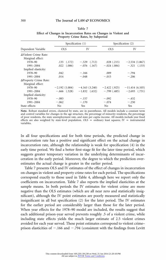
300 The Journal of LAW& ECONOMICS
Table 7
Effect of Changes in Incarceration Rates on Changes in Violent andProperty Crime Rates, by Subperiod
Specification (1) Specification (2)
Dependent Variable OLS IV OLS IV
DViolent Crime Rate:Marginal effect:
1978–90 .135 (.172) �.529 (.712) .028 (.215) �2.534 (1.867)1991–2004 .022 (.086) �.076 (.167) �.024 (.084) �.321 (.133)
Implied elasticity:1978–90 .042 �.166 .009 �.7941991–2004 .014 �.048 �.015 �.206
DProperty Crime Rate:Marginal effect:
1978–90 �2.192 (1.004) �4.163 (3.240) �2.422 (.925) �11.414 (6.105)1991–2004 �.666 (.528) �1.832 (.632) �.799 (.485) �2.693 (.731)
Implied elasticity:1978–90 �.083 �.157 �.092 �.4321991–2004 �.062 �.170 �.074 �.250
State effects No Yes No Yes
Note. Robust standard errors, clustered by state, are in parentheses. All models include a constant termand control variables for changes in the age structure, the percentage of minority residents, the percentageof poor residents, the state unemployment rate, and state per capita income. All models include year fixedeffects are also weighted by state-level population. OLS p ordinary least squares; IV p instrumentalvariables.
In all four specifications and for both time periods, the predicted change inincarceration rate has a positive and significant effect on the actual change inincarceration rate, although the relationship is weak for specification (4) in theearly time period. We find a better first-stage fit for the later time period, whichsuggests greater temporary variation in the underlying determinants of incar-ceration in the early period. Moreover, the degree to which the prediction over-estimates the actual change is greater in the earlier period.
Table 7 presents OLS and IV estimates of the effect of changes in incarcerationon changes in violent and property crime rates for each period. The specificationscorrespond exactly to those used in Table 4, although here we report only thecoefficients on incarceration. Table 7 also reports the implied elasticities at thesample means. In both periods the IV estimates for violent crime are morenegative than the OLS estimates (which are all near zero and statistically insig-nificant), although the IV point estimates are poorly measured and statisticallyinsignificant in all but specification (2) for the later period. The IV estimatesfor the earlier period are considerably larger than those for the later period.When year effects for the 1978–90 model are included, the results suggest thateach additional prison-year served prevents roughly .5 of a violent crime, whileincluding state effects yields the much larger estimate of 2.5 violent crimesavoided for each year served. These point estimates correspond to violent crime–prison elasticities of �.166 and �.794 (consistent with the findings from Levitt
This content downloaded from 169.229.139.238 on Wed, 25 Jun 2014 21:20:18 PMAll use subject to JSTOR Terms and Conditions
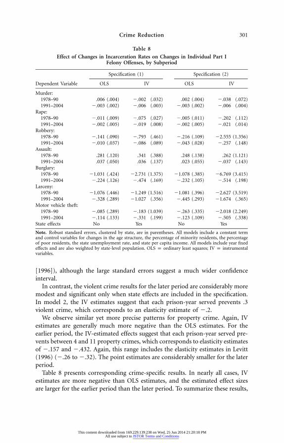
Crime Reduction 301
Table 8
Effect of Changes in Incarceration Rates on Changes in Individual Part IFelony Offenses, by Subperiod
Specification (1) Specification (2)
Dependent Variable OLS IV OLS IV
Murder:1978–90 .006 (.004) �.002 (.032) .002 (.004) �.038 (.072)1991–2004 �.003 (.002) �.006 (.003) �.003 (.002) �.006 (.004)
Rape:1978–90 �.011 (.009) �.075 (.027) �.005 (.011) �.202 (.112)1991–2004 �.002 (.005) �.019 (.008) �.002 (.005) �.021 (.014)
Robbery:1978–90 �.141 (.090) �.793 (.461) �.216 (.109) �2.555 (1.356)1991–2004 �.010 (.037) �.086 (.089) �.043 (.028) �.257 (.148)
Assault:1978–90 .281 (.120) .341 (.388) .248 (.138) .262 (1.121)1991–2004 .037 (.050) .036 (.137) .023 (.055) �.037 (.143)
Burglary:1978–90 �1.031 (.424) �2.731 (1.375) �1.078 (.385) �6.769 (3.415)1991–2004 �.224 (.126) �.474 (.169) �.232 (.105) �.514 (.198)
Larceny:1978–90 �1.076 (.446) �1.249 (1.516) �1.081 (.396) �2.627 (3.519)1991–2004 �.328 (.289) �1.027 (.356) �.445 (.293) �1.674 (.365)
Motor vehicle theft:1978–90 �.085 (.289) �.183 (1.039) �.263 (.335) �2.018 (2.249)1991–2004 �.114 (.133) �.331 (.199) �.123 (.109) �.505 (.338)
State effects No Yes No Yes
Note. Robust standard errors, clustered by state, are in parentheses. All models include a constant termand control variables for changes in the age structure, the percentage of minority residents, the percentageof poor residents, the state unemployment rate, and state per capita income. All models include year fixedeffects and are also weighted by state-level population. OLS p ordinary least squares; IV p instrumentalvariables.
[1996]), although the large standard errors suggest a much wider confidenceinterval.
In contrast, the violent crime results for the later period are considerably moremodest and significant only when state effects are included in the specification.In model 2, the IV estimates suggest that each prison-year served prevents .3violent crime, which corresponds to an elasticity estimate of �.2.
We observe similar yet more precise patterns for property crime. Again, IVestimates are generally much more negative than the OLS estimates. For theearlier period, the IV-estimated effects suggest that each prison-year served pre-vents between 4 and 11 property crimes, which corresponds to elasticity estimatesof �.157 and �.432. Again, this range includes the elasticity estimates in Levitt(1996) (�.26 to �.32). The point estimates are considerably smaller for the laterperiod.
Table 8 presents corresponding crime-specific results. In nearly all cases, IVestimates are more negative than OLS estimates, and the estimated effect sizesare larger for the earlier period than the later period. To summarize these results,
This content downloaded from 169.229.139.238 on Wed, 25 Jun 2014 21:20:18 PMAll use subject to JSTOR Terms and Conditions
302 The Journal of LAW& ECONOMICS
we again estimate the total number of crimes avoided by an additional prison-year served, adjusted for crime-specific underreporting rates in the UCR data.To do so, we make use of the estimation results in the final column of Table 8,which uses the most liberal specification of the IV model. The results indicatethat for the period 1978–90, each additional inmate prevented approximately 30part I felony offenses. The comparable value for the period 1991–2004 is 8.3.Thus, the marginal crime-fighting effect of an additional inmate has indeeddeclined substantially in recent years.
7. Conclusion
This study has several important findings and contributions. First, to isolateexogenous variation in incarceration, we use the dynamic adjustment path ofaggregate incarceration rates induced by shocks to underlying determinants ofincarceration rates. Our theoretical prediction regarding subsequent 1-yearchanges in incarceration rates provides a strong instrument for actual changesin incarceration rates. Moreover, the strategy permits us to estimate separateeffects for the United States, stratified by period, because the instrument doesnot depend on variation in specific states or periods.
Second, we find that breaking the simultaneity between incarceration andcrime rates yields substantially larger estimates of the effects of incarceration oncrime than those estimated in simple OLS models. When restricted to earlierperiods, our corrected estimates are in accord with those of Levitt (1996), whoanalyzes a similar period yet uses an entirely different identification strategy.
Third, we find that the effect on crime rates of incarcerating one more inmatehas declined drastically over the past quarter century. When we split the sampleinto two equal periods, we find crime-prison effects for the later period that areless than one-third the size of those for the earlier period. For 1978–90, weestimate that each additional prison-year served prevented approximately 30index crimes. For the period 1991–2004, the comparable value is eight. Moreover,this decline in level effects corresponds to substantial declines in crime-prisonelasticities, which suggests that the constant-elasticity specification often used inprevious research underestimates the degree to which the crime-abating effectsof incarceration decrease with scale.
This large decline in the marginal effect of an inmate suggests that the mostrecent increases in incarceration have been driven by the institutionalization ofmany inmates who, relative to previous periods, pose less of a threat to society.Indeed, given the much lower crime-abating effects for the most recent period,it is likely the case that for many recent inmates, the benefits to society in termsof crime reduction are unlikely to outweigh the explicit monetary costs of housingand maintaining an additional inmate. Moreover, once we accounts for theadditional external costs of incarceration, such as the adverse effects on thefamilies of inmates, the effects on victimizations behind bars, the effects on
This content downloaded from 169.229.139.238 on Wed, 25 Jun 2014 21:20:18 PMAll use subject to JSTOR Terms and Conditions
Crime Reduction 303
additional HIV/AIDS infections (Johnson and Raphael 2010), and the potentialeffects on the long-term employment prospects of former inmates, the benefit-cost ratio on the margin is likely to be substantially less than one.
Appendix
Incorporating Behavioral Responses into theModel of Incarceration and Crime
The model presented in Section 3 assumes that the underlying transitionparameters in our aggregate model of crime and incarceration do not respondto one another, either instantaneously or with a dynamic lag. Here we sequentiallyrelax some of the behavioral assumptions that we made and assess how thisimpacts the interpretation of our results.
We first maintain the assumption that underlying criminality is unresponsiveto either the threat of incarceration (captured by p) or the severity of punishment(captured by the release parameter v). We begin by considering the case in whichthe likelihood of being apprehended and incarcerated varies with the degree ofunderlying criminality—that is, where . One might hypothesize a priorip p p(c)that p may be either increasing or decreasing in the degree of criminality. Ifpolicy makers respond to an increase in criminal behavior by greatly increasingresources devoted to policing and corrections, we would expect that increasesin criminality would lead to increases in the risk of incarceration. On the otherhand, to the extent that increases in criminality dilute enforcement resources,
may be negative.dp/dcWith regard to our identification strategy, in isolation such a policy reaction
should not compromise the exogeneity of our proposed instrument, althoughthe timing of this response may impact the strength of our first-stage relationship.To see this, first consider the case in which p responds instantaneously to changesin c. For , an increase in criminality will cause an instantaneous increasedp/dc 1 0in the incarceration risk. The higher value of p will translate into a lower initialspike in crime, a larger initial increase in incarceration, and a speedier adjustmentof incarceration and crime rates to their new equilibrium levels. The oppositewould apply when p decreases in c. In either case, the change in incarcerationrate subsequent to the initial change still provides exogenous variation in in-carceration and thus the IV strategy outlined above still identifies a causal in-capacitation effect.
However, the incarceration risk parameter is unlikely to respond instanta-neously, since policy makers are likely to learn of an increase in c only with timeand since the budgetary process impedes instantaneous reaction to new problems.Such a delayed response will impact the first-stage relationship between thepredicted change in incarceration in equation (10) and actual changes. To seethis, suppose that at the risk of incarceration is but that it increases tot p 0 p0
at the beginning of period 1 (fully 1 period after the increase in criminalityp1
This content downloaded from 169.229.139.238 on Wed, 25 Jun 2014 21:20:18 PMAll use subject to JSTOR Terms and Conditions
304 The Journal of LAW& ECONOMICS
modeled above). Given that the incarceration risk remained constant for the firstperiod following the shock, the initial change in the incarceration rate remainsequal to that described in the first line of equation (10). However, the newincrease in incarceration between periods 1 and 2 becomes
DS p D � (S* � S* )(c p � v)S2,1 2,2 2,1 1 0 2,1Fconstant p (A1)
� c (p � p )(S* � S ),1 1 0 2,2 2,1
where the first term is the predicted change in incarceration holding the incar-ceration risk constant (the second line in equation [10] and our proposed in-strument), is the new long-run equilibrium incarcerationS* p c p /(c p � v)2,2 1 1 1 1
rate with the elevated incarceration risk, is the equilibriumS* p c p /(c p � v)2,1 1 0 1 0
incarceration rate given last period’s parameters, and is the actual incarcer-S2,1
ation rate in period 1. The second term in equation (A1) adjusts our previousestimate of the increase in incarceration for this period for the change in thelong-term equilibrium rate, while the third terms reflects the instantaneous effectof the increase in the incarceration risk parameter p. When p is increasing in c,both terms are positive. Thus, our proposed instrument will systematically un-derestimate the actual change in incarceration rate. If p is a decreasing functionof c, then the opposite would hold. Regardless, our proposed instrument is stilla component of the change in incarceration rate, and thus a first-stage rela-tionship should exist. Moreover, because the criminality parameter is assumedto be constant across periods, this particular behavioral response will not inducecorrelation between the instrument and the second-stage error term.
The impact of a change in sentence length on our instrument requires adynamics analysis, since a change in sentence length today will not impactchanges in incarceration rates until today’s cohort of admitted inmates reachestheir counterfactual release dates under the prior sentencing regime. In practice,inmates sentenced to state or federal prison receive sentences of at least 1 year,although those being sent back for parole violation often serve terms that mayfall short of a full year (Raphael and Weiman 2008). Here we work through theeffect of an increase in sentence length in response to an increase in criminality,operating under the assumption that an increase in c at time does nott p 0impact release rates until .t p 1
If policy makers increase sentence severity in response to an increase in crim-inality, this implies that period release rates decrease in the once-lagged valueof c, or . Again, since v does not change instantaneously in response′
v (c ) ! 0t t�1
to a change in the criminality parameter, the period 1 change in incarcerationrates will not differ from that in the first line of equation (10). The change inincarceration between periods 1 and 2, however, will differ by an identifiablequantity. To be specific, assuming that the release probability increases from
at to at , the implied change in the incarceration rate betweenv t p 0 v t p 10 1
periods 1 and 2 will be
This content downloaded from 169.229.139.238 on Wed, 25 Jun 2014 21:20:18 PMAll use subject to JSTOR Terms and Conditions
Crime Reduction 305
DS p DS � (v � v )S . (A2)2,1 2,1Fconstant v 0 1 2,1
The first term on the right-hand side of equation (A2) is our previous estimateof the period change in incarceration rates, assuming no responsiveness of v tochanges in c, while the second term reflects an additional component associatedwith the lower release rate at (which will be positive for ). Thus,t p 1 v ! v1 0
allowing sentence severity to respond punitively to increases in criminality sug-gests that our proposed instrument will underestimate the increase in incarcer-ation. Nonetheless, the instrument again predicts a component of the changeand thus should be able to identify significant variation in the future change inincarceration rates. Moreover, we are holding the criminality parameter constantby assumption, and thus the instrument will not be correlated with the errorterm in the second-stage equation.
Allowing criminality and corrections policy to respond reciprocally complicatesthe analysis somewhat and does indeed bias the second-stage estimate of ourstructural estimate of the effect of incarceration on crime, if we interpret thisestimate narrowly as a pure incapacitation effect. However, if we broaden theinterpretation of the effect that we are estimating to allow for a general deterrenceeffect in addition to an incapacitation effect, our instrument is still valid. To seethis, we begin with a simple model whereby criminality and enforcement adjustinstantaneously to one another. We then think through a likely dynamic structureof this response and how it will impact our estimation strategy.
Suppose that criminality is determined by two factors: a variable x measuringcriminogenic influences that are unresponsive to policy and the overall incar-ceration risk p. Assume further that criminality is determined according to theadditively separable function , where and . We′ ′c p h(x) � f(p) h (x) 1 0 f (p) ! 0also assume that the incarceration risk is a monotonically increasing functionof the criminality parameter —that is, , where�1h(x) � f(p) p g (p) p p g(c)
. The assumption that p is increasing in c best describes the recent history′g (c) 1 0of corrections policy in the United States.16 The equilibrium incarceration riskis defined by the condition
�1h(x) � f(p) p g (p), (A3)
where is the inverse of the function . Totally differentiating condition�1g (p) g(c)(A3) with respect to x and the equation for c gives the response of p and c inresponse to a change in x:
16 The period with perhaps the strongest evidence in favor of an overall increase in criminalityoccurred during the later 1980s and early 1990s (the period corresponding to the crack cocaineepidemic). During that period, prison admission rates increased steeply relative to previous levels,and sentences were enhanced at the federal level and in many states for nonviolent drug crimes andfor other felony offenses. For detailed discussions of sentencing policy in the United States, see Tonry(1996) and Jacobson (2006).
This content downloaded from 169.229.139.238 on Wed, 25 Jun 2014 21:20:18 PMAll use subject to JSTOR Terms and Conditions
306 The Journal of LAW& ECONOMICS
′dp h (x)p ,′ ′�1dx g (x) � f (p) (A4)
′dc f (p)′p h (x) 1 � .′ ′[ ]�1dx g (p) � f (p)
For , both derivatives in equation (A4) are positive. Thus, a positive′g (c) 1 0shock to underlying crime fundamentals leads to an equilibrium increase in bothcriminality and the incarceration risk.
The implications of this bidirectional responsiveness for our identificationstrategy will again depend on whether these adjustments occur instantaneouslyor over time. If a shock to c causes an instantaneous adjustment of the incar-ceration risk and criminality to new equilibrium levels, then our identificationstrategy is not affected. Future increases in incarceration will be based on stablebehavioral and policy parameters, and our proposed instrument will identifyexogenous variation in future changes in incarceration rates.
However, the reaction of policy to a change in criminality is likely to be slowerthan the reaction of criminal behavior to changes in enforcement, since changesin policy will be slowed to some degree by the timing of the budgetary process.Moreover, if policy makers choose an optimal enforcement level based on theirbest estimate of current criminality, equilibrium values of p and c may not bereached after only a multiperiod adjustment process. Here we consider the im-plications for our identification strategy of the specialized case where c respondsinstantaneously to changes in p but where p responds to changes in c with a 1-period lag. Since our chosen instrument will be used to predict changes inincarceration between periods and , we consider only the effect oft p 1 t p 2this reciprocal responsiveness for the first two changes in crime and incarcerationrates following a shock to c.
Assume that at , criminality increases from to . Given the laggedt p 0 c c0 1
responsiveness of the incarceration risk, p will not increase until period 1. Atthat time, the parameter increases from to . Since criminality respondsp p0 1
instantaneously, the criminality parameter will decrease from to , as suggestedc c1 2
by the simple model in equations (A3) and (A4).17 For this example, the firsttwo changes in observed crime rates are given by the equations
DC p �c DS � (c � c )(1 � S* )0 1 2,0 1 0 2,0 (A5)
DC p �c DS � (c � c )(1 � S ).1 2 2,1 2 1 2,1
Note that the change in the crime rate between periods 0 and 1 is equivalentto the change reported in equation (11), where we assumed away behavioral
17 To be sure, will not be an equilibrium value for criminality but rather the optimal behavioralc2
response to the incarceration risk associated with . It will take several additional policy iterationsp1
and reciprocal behavioral responses to reach steady-state values for the parameters. However, sincewe are primarily interested in instrumenting the change in incarceration between periods 1 and 2,we do not need to consider subsequent changes.
This content downloaded from 169.229.139.238 on Wed, 25 Jun 2014 21:20:18 PMAll use subject to JSTOR Terms and Conditions
Crime Reduction 307
responses of the parameters. The change in crime rates between periods 1 and2, however, has changed, with an alternative coefficient on the change in in-carceration ( instead of ) and an additional term capturing the effect on�c �c2 1
crime of the decrease in criminality from to . This second term is basicallyc c1 2
the general deterrence effect of an increase in the incarceration risk.Since we cannot observe the actual values for the criminality parameter, this
general deterrence component will be swept into the error term in the second-stage crime equation (given by the second line in equation [A5]). Since thedecreases in criminality in period 1 are driven by the response of policy to theincreases in criminality in period 0, the change in criminality between periods0 and 1 will be negatively correlated with the change in criminality betweenperiods 1 and 2. Our proposed instrument is increasing in the initial increasein criminality. Thus, our instrument will be negatively correlated with the de-terrence effect contained in the error term of the second-stage regression, whichcauses a negative bias to our estimate of the incapacitation effect of prison (thatis, our elasticity estimates will be too large).
Despite this change, however, we are still able to interpret the structural es-timate from the second stage as a causal effect of corrections policy on crime,although we must change our interpretation somewhat. With a lagged reciprocalresponse, the second-stage estimate of the coefficient on the change in incar-ceration will reflect both the incapacitation effect and the general deterrenceeffect of prison on crime (through the correlation between the predicted incar-ceration change and the general deterrence component in the error term). Thus,although we are unable to disentangle the separate avenues by which prison islikely to impact criminality activity, our proposed IV estimate does permit es-timation of a cumulative impact.
With regard to our first-stage prediction, the predicted increase in incarcerationwith stable parameters may either overestimate or underestimate the actual in-crease. With the stated sequence of criminality and incarceration risk valueslisted above, the actual increase in incarceration between periods 1 and 2 is givenby the equation
DS p DS � (S* � S*)(c p � v) � (S* � S )(c p � c p ), (A6)2,1 2,1Fconstant p, c 2 1 1 0 2 1 2 1 1 0
where the first term is the predicted change in incarceration between periods 1and 2, assuming stable parameters following the initial crime shock, where
is the new equilibrium incarceration rate after the periodS* p c p /(c p � v)2 2 1 2 1
1 response of criminality to the change in the incarceration risk, S* p1
is the equilibrium rate after the initial criminality shock butc p /(c p � v)1 0 1 0
preceding the incarceration risk response, and is the actual incarceration rateS1
at the beginning of period 1. The second and third terms in this model willboth be either positive or negative depending on the relative size of andc p2 1
. If , the increase in the incarceration risk is so large relative toc p c p 1 c p1 0 2 1 1 0
the subsequent decrease in criminality that the equilibrium incarceration rateincreases. In this instance, the instrument will underestimate the actual increase
This content downloaded from 169.229.139.238 on Wed, 25 Jun 2014 21:20:18 PMAll use subject to JSTOR Terms and Conditions
308 The Journal of LAW& ECONOMICS
in incarceration. On the other hand, if , then the decline in criminalityc p ! c p2 1 1 0
is sufficiently large relative to the increase in the incarceration risk that theequilibrium rate declines and both of the second terms in equation (A6) arenegative. In this instance, our nonbehavioral prediction will overestimate theactual change in the incarceration rate.
There is one potential behavioral response on the part of the potentiallycriminal that may bias our results, even when interpreted to represent a totaleffect of incarceration on crime. Suppose that current increases in criminalbehavior cause subsequent decreases in criminality because of a revulsion onthe part of the general public to the consequences of the crime spike. Suchresponses suggest that changes in the criminality parameter may exhibit negativeserial correlation. An example of such a revulsion effect may be a drug epidemicthat runs it course when a younger generation is reluctant to use a drug thatdevastated the lives of the preceding generation. This type of serial correlationwould create a negative correlation between our instrument and the correspond-ing change in the crime rate, for reasons similar to those given in the discussionof equation (A6). Here however, the decline in the crime rate cannot be attributedto a general deterrence effect of prison, since the decline would occur regardlessof a change in the chance of punishment. In this case, there would be a spuriousreduced-form relationship between the instrument and the change in the crimerate.
Although such changes in behavior are certainly possible, that spikes in crim-inal behavior driven by the introduction of a new drug or other variants ofcrime shocks would correct themselves within a year or two is unlikely andcontrary to recent history. Nonetheless, we acknowledge this threat to the validityof our estimation strategy.
This content downloaded from 169.229.139.238 on Wed, 25 Jun 2014 21:20:18 PMAll use subject to JSTOR Terms and Conditions
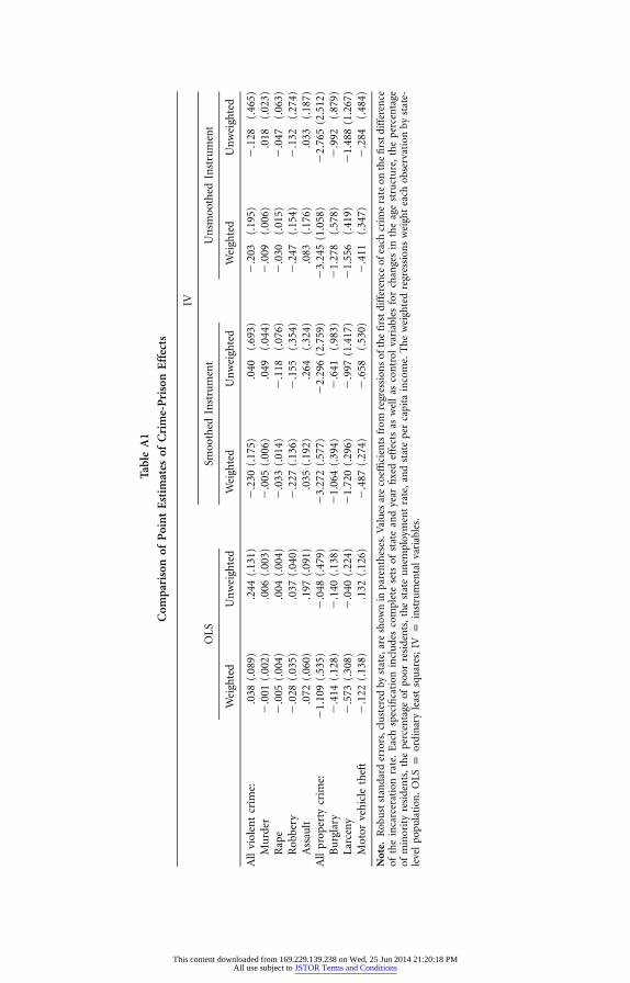
Tabl
eA
1
Com
pari
son
ofP
oin
tE
stim
ates
ofC
rim
e-P
riso
nE
ffec
ts
IV
OL
SSm
ooth
edIn
stru
men
tU
nsm
ooth
edIn
stru
men
t
Wei
ghte
dU
nw
eigh
ted
Wei
ghte
dU
nw
eigh
ted
Wei
ghte
dU
nw
eigh
ted
All
viol
ent
crim
e:.0
38(.
089)
.244
(.13
1)�
.230
(.17
5).0
40(.
693)
�.2
03(.
195)
�.1
28(.
465)
Mu
rder
�.0
01(.
002)
.006
(.00
3)�
.005
(.00
6).0
49(.
044)
�.0
09(.
006)
.018
(.02
3)R
ape
�.0
05(.
004)
.004
(.00
4)�
.033
(.01
4)�
.118
(.07
6)�
.030
(.01
5)�
.047
(.06
3)R
obbe
ry�
.028
(.03
5).0
37(.
040)
�.2
27(.
136)
�.1
55(.
354)
�.2
47(.
154)
�.1
32(.
274)
Ass
ault
.072
(.06
0).1
97(.
091)
.035
(.19
2).2
64(.
324)
.083
(.17
6).0
33(.
187)
All
prop
erty
crim
e:�
1.10
9(.
535)
�.0
48(.
479)
�3.
272
(.57
7)�
2.29
6(2
.759
)�
3.24
5(1
.058
)�
2.76
5(2
.512
)B
urg
lary
�.4
14(.
128)
�.1
40(.
138)
�1.
064
(.39
4)�
.641
(.98
3)�
1.27
8(.
578)
�.9
92(.
879)
Larc
eny
�.5
73(.
308)
�.0
40(.
224)
�1.
720
(.29
6)�
.997
(1.4
17)
�1.
556
(.41
9)�
1.48
8(1
.267
)M
otor
veh
icle
thef
t�
.122
(.13
8).1
32(.
126)
�.4
87(.
274)
�.6
58(.
530)
�.4
11(.
347)
�.2
84(.
484)
Not
e.R
obu
stst
anda
rder
rors
,clu
ster
edby
stat
e,ar
esh
own
inpa
ren
thes
es.V
alu
esar
eco
effi
cien
tsfr
omre
gres
sion
sof
the
firs
tdi
ffer
ence
ofea
chcr
ime
rate
onth
efi
rstd
iffe
ren
ceof
the
inca
rcer
atio
nra
te.
Eac
hsp
ecifi
cati
onin
clu
des
com
plet
ese
tsof
stat
ean
dye
arfi
xed
effe
cts
asw
ell
asco
ntr
olva
riab
les
for
chan
ges
inth
eag
est
ruct
ure
,th
epe
rcen
tage
ofm
inor
ity
resi
den
ts,
the
perc
enta
geof
poor
resi
den
ts,
the
stat
eu
nem
ploy
men
tra
te,
and
stat
epe
rca
pita
inco
me.
Th
ew
eigh
ted
regr
essi
ons
wei
ght
each
obse
rvat
ion
byst
ate-
leve
lpo
pula
tion
.O
LSp
ordi
nar
yle
ast
squ
ares
;IV
pin
stru
men
tal
vari
able
s.
This content downloaded from 169.229.139.238 on Wed, 25 Jun 2014 21:20:18 PMAll use subject to JSTOR Terms and Conditions
310 The Journal of LAW& ECONOMICS
References
Cameron, A. Colin, and Pravin K. Trivedi. 2005. Microeconometrics: Methods and Appli-cations. New York: Cambridge University Press.
DiIulio, John J., and Anne Piehl. 1991. Does Prison Pay? The Stormy National Debateover the Cost-Effectiveness of Imprisonment. Brookings Review 9(4):28–35.
Donohue, John J., III, and Peter Siegelman. 1998. Allocating Resources among Prisonsand Social Programs in the Battle against Crime. Journal of Legal Studies 27:1–43.
Drago, Francesco, Roberto Galbiati, and Pietro Vertova. 2009. The Deterrent Effects ofPrison: Evidence from a Natural Experiment. Journal of Political Economy 117:257–80.
Jacobson, Michael. 2005. Downsizing Prisons: How to Reduce Crime and End Mass Incar-ceration. New York: New York University Press.
Johnson, Rucker, and Steven Raphael. 2010. The Effect of Male Incarceration Dynamicson AIDS Infection Rates among African-American Women and Men. Journal of Lawand Economics 52:251–93.
Kessler, Daniel, and Steven D. Levitt. 1999. Using Sentence Enhancements to Distinguishbetween Deterrence and Incapacitation. Journal of Law and Economics 42:343–63.
Lee, David S., and Justin McCrary. 2005. Crime, Punishment, and Myopia. Working PaperNo. 11491. National Bureau of Economic Research, Cambridge, Mass.
Levitt, Steven D. 1996. The Effect of Prison Population Size on Crime Rates: Evidencefrom Prison Overcrowding Legislation. Quarterly Journal of Economics 111:319–51.
———. 1998. Juvenile Crime and Punishment. Journal of Political Economy 106:1156–85.
Marvell, Thomas, and Carlysle Moody. 1994. Prison Population Growth and Crime Re-duction. Journal of Quantiative Criminology 10:109–40.
Owens, Emily G. 2009. More Time, Less Crime? Estimating the Incapacitative Effects ofSentence Enhancements. Journal of Law and Economics 52:551–79.
Raphael, Steven, and David Weiman. 2008. The Impact of Local Labor Market Conditionson the Likelihood That Parolees Are Returned to Custody. Pp. 304–22 in Barriers toReentry? The Labor Market for Released Prisoners in Post-industrial America, edited byShawn Bushway, Michael A. Stoll, and David F. Weiman. New York: Russell SageFoundation.
Rennison, Callie M. 2001. Criminal Victimization 2000: Changes 1999–2000 with Trends1993–2000. NCJ 187007. Washington, D.C.: Bureau of Justice Statistics.
Spelman, William. 1994. Criminal Incapacitation. New York: Plenum Press.———. 2000. What Recent Studies Do (and Don’t) Tell Us about Imprisonment and
Crime. Pp. 419–94 in Crime and Justice: A Review of the Research, edited by MichaelTonry. Chicago: University of Chicago Press.
Tonry, Michael. 1996. Sentencing Matters. Oxford: Oxford University Press.Webster, Cheryl M., Anthony N. Doob, and Franklin E. Zimring. 2006. Proposition 8
and Crime Rates in California: The Case of the Disappearing Deterrent. Criminologyand Public Policy 5:417–48.
Western, Bruce. 2006. Punishment and Inequality in America. New York: Russell SageFoundation.
This content downloaded from 169.229.139.238 on Wed, 25 Jun 2014 21:20:18 PMAll use subject to JSTOR Terms and Conditions