Embed Size (px)
Citation preview
The Bayesian Bridge
Nicholas G. Polson
University of Chicago∗
James G. Scott
Jesse Windle
University of Texas at Austin
First Version: July 2011This Version: October 2012
Abstract
We develop the Bayesian bridge estimator for regularized regression and classification.We focus on two distinct mixture representations for the prior distribution that giverise to the Bayesian bridge model: (1) a scale mixture of normals with respect to analpha-stable random variable; and (2) a mixture of Bartlett–Fejer kernels (or triangledensities) with respect to a two-component mixture of gamma random variables. Thefirst representation is a well known result due to West (1987), and is the more efficientchoice for collinear design matrices. The second representation is new, and is moreefficient for orthogonal problems, largely by avoiding the need to deal with exponentiallytilted stable random variables. It also provides insight into the multimodality of the jointposterior distribution, a feature of the bridge model that is notably absent under ridgeor lasso-type priors (Park and Casella, 2008; Hans, 2009). We find that the Bayesianbridge model outperforms its classical cousin in estimation and prediction across avariety of data sets, both simulated and real. We also prove a theorem that extends theapproach to a wider class of regularization penalties that can be represented as scalemixtures of betas, and provide an explicit inversion formula for the mixing distribution.Finally, we show that the MCMC for fitting the bridge model has the striking propertyof generating nearly independent draws for the global scale parameter. This makes itfar more efficient than analogous MCMC algorithms for fitting other sparse Bayesianmodels.
∗Polson is Professor of Econometrics and Statistics at the Chicago Booth School of Business. email:[email protected]. Scott is Assistant Professor of Statistics at the University of Texas at Austin.email: [email protected]. Windle is a Ph.D student at the University of Texas at Austin.email: [email protected].
1
1 Introduction
1.1 Penalized likelihood and the Bayesian bridge
This paper studies the Bayesian analogue of the bridge estimator in regression, where y =Xβ + ε for some unknown vector β = (β1, . . . , βp)′. Given choices of α ∈ (0, 1] and ν ∈ R+,the bridge estimator β is the minimizer of
Qy(β) =12||y −Xβ||2 + ν
p∑j=1
|βj |α . (1)
This bridges a class of shrinkage and selection operators, with the best-subset-selectionpenalty at one end, and the `1 (or lasso) penalty at the other. An early reference to thisclass of models can be found in Frank and Friedman (1993), with recent papers focusingon model-selection asymptotics, along with strategies for actually computing the estimator(Huang et al., 2008; Zou and Li, 2008; Mazumder et al., 2011).
Our approach differs from this line of work in adopting a Bayesian perspective on bridgeestimation. Specifically, we treat p(β | y) ∝ exp−Qy(β) as a posterior distribution havingthe minimizer of (1) as its global mode. This posterior arises in assuming a Gaussianlikelihood for y, along with a prior for β that decomposes as a product of independentexponential-power priors (Box and Tiao, 1973):
p(β | α, ν) ∝p∏j=1
exp(−|βj/τ |α) , τ = ν−1/α . (2)
Rather than minimizing (1), we proceed by constructing a Markov chain having the jointposterior for β as its stationary distribution.
1.2 Relationship with previous work
Our paper emphasizes several interesting features of the Bayesian approach to bridge esti-mation. We summarize these features here, grouping them into three main categories.
Versus the Bayesian ridge and lasso priors. There is a large literature on Bayesianversions of classical estimators related to the exponential-power family, including the ridge(Lindley and Smith, 1972), lasso (Park and Casella, 2008; Hans, 2009, 2010), and elasticnet (Li and Lin, 2010; Hans, 2011). Yet the bridge penalty has a crucial feature not sharedby these other approaches: it is concave over (0,∞). From a Bayesian perspective, thisimplies that the prior for β has heavier-than-exponential tails. As a result, when theunderlying signal is sparse, and when further regularity conditions are met, the bridgepenalty dominates the lasso and ridge according to a classical criterion known as the oracleproperty (Fan and Li, 2001; Huang et al., 2008). Although the oracle property per seis of no particular relevance to a Bayesian treatment of the problem, it does correspondto a feature of certain prior distributions that Bayesians have long found important: theproperty of yielding a redescending score function for the marginal distribution of y (e.g.
2
Pericchi and Smith, 1992). This property is highly desirable in sparse situations, as it avoidsthe overshrinkage of large regression coefficients even in the presence of many zeros (Polsonand Scott, 2011a).
Versus the classical bridge estimator. Both the classical and Bayesian approaches tobridge estimation must confront a significant practical difficulty: exploring and summarizinga multimodal surface in high-dimensional Euclidean space. In our view, multimodalityis one of the strongest arguments for pursuing a full Bayes approach. For one thing, itis misleading to summarize a multimodal surface in terms of a single point estimate, nomatter how appealingly sparse that estimate may be. Moreover, Mazumder et al. (2011)report serious computational difficulties with getting stuck in local modes in attemptingto minimize (1). Our sampling-based approach, while not immune to this difficulty, seemsvery effective at exploring the whole space. (As Section 2 will show, there are very goodreasons for expecting this to be the case, based on the structure of the data-augmentationstrategy we pursue.) In this respect, MCMC behaves like a simulated annealing algorithmthat never cools.
In addition, previous authors have emphasized three other points about penalized-likelihood rules that will echo in the examples we present in Section 4. First, one mustchoose a penalty parameter ν. In the classical setting this can be done via cross valida-tion, which usually yields reasonable results. Yet this ignores uncertainty in the penaltyparameter, which may be considerable. We are able to handle this in a principled way byaveraging over uncertainty in the posterior distribution, under some default prior for theglobal variance component τ2 (e.g. Gelman, 2006; Polson and Scott, 2012b). In the caseof the bridge estimator, this logic may also be extended to the concavity parameter α, forwhich even less prior information is typically available.
Second, the minimizer of (1) may produce a sparse estimator, but this estimate isprovably suboptimal, in a Bayes-risk sense, with respect to most traditional loss functions.If, for example, one wishes either to estimate β or to predict future values of y undersquared-error loss, then the optimal solution is the posterior mean, not the mode. BothPark and Casella (2008) and Hans (2009) give realistic examples where the “Bayesian lasso”significantly outperforms its classical counterpart, both in prediction and in estimation.Similar conclusions are reached by Efron (2009) in a parallel context. Our own examplesprovide evidence of the practical differences that arise on real data sets—not merely betweenthe mean and the mode, but also between the classical bridge solution and the mode of thejoint distribution in the Bayesian model, marginal over over τ and σ. In the cases we study,the Bayesian approach leads to lower risk, often dramatically so.
Third, a fully Bayesian approach can often lead to different substantive conclusions thana traditional penalized-likelihood analysis, particularly regarding which components of β areimportant in predicting y. For example, Hans (2010) produces several examples where theclassical lasso estimator aggressively zeroes out components of β for which, according to afull Bayes analysis, there is quite a large amount of posterior uncertainty regarding theirsize. This is echoed in our analysis of the classic data set on diabetes in Pima Indians.This is not to suggest that one conclusion is right, and the other wrong, in any specific
3
setting—merely that the two conclusions can be quite different, and that practitioners arewell served by having both at hand.
Versus other sparsity-inducing priors in Bayesian regression analysis. Withinthe broader class of regularized estimators in high-dimensional regression, there has beenwidespread interest in cases where the penalty function corresponds to a normal scale mix-ture. Many estimators in this class share the favorable sparsity-inducing property (i.e. heavytails) of the Bayesian bridge model. This includes the relevance vector machine of Tipping(2001); the normal/Jeffreys model of Figueiredo (2003) and Bae and Mallick (2004); thenormal/exponential-gamma model of Griffin and Brown (2012); the normal/gamma andnormal/inverse-Gaussian (Caron and Doucet, 2008; Griffin and Brown, 2010); the horse-shoe prior of Carvalho et al. (2010); and the double-Pareto model of Armagan et al. (2012).
In virtually all of these models, the primary difficulty is the mixing rate of the MCMCused to sample from the joint posterior for β. Most MCMC approaches in this realm uselatent variables to make sampling convenient. But this can lead to poor mixing rates,especially in cases where the fraction of “missing information”—that is, the information inthe conditional distribution for β introduced by the latent variables—is large. Section 3.3of the paper by Hans (2009) contains an informative discussion of this point. We have alsoincluded an online supplement to the manuscript that extensively documents the mixingbehavior of Gibbs samplers within this realm.
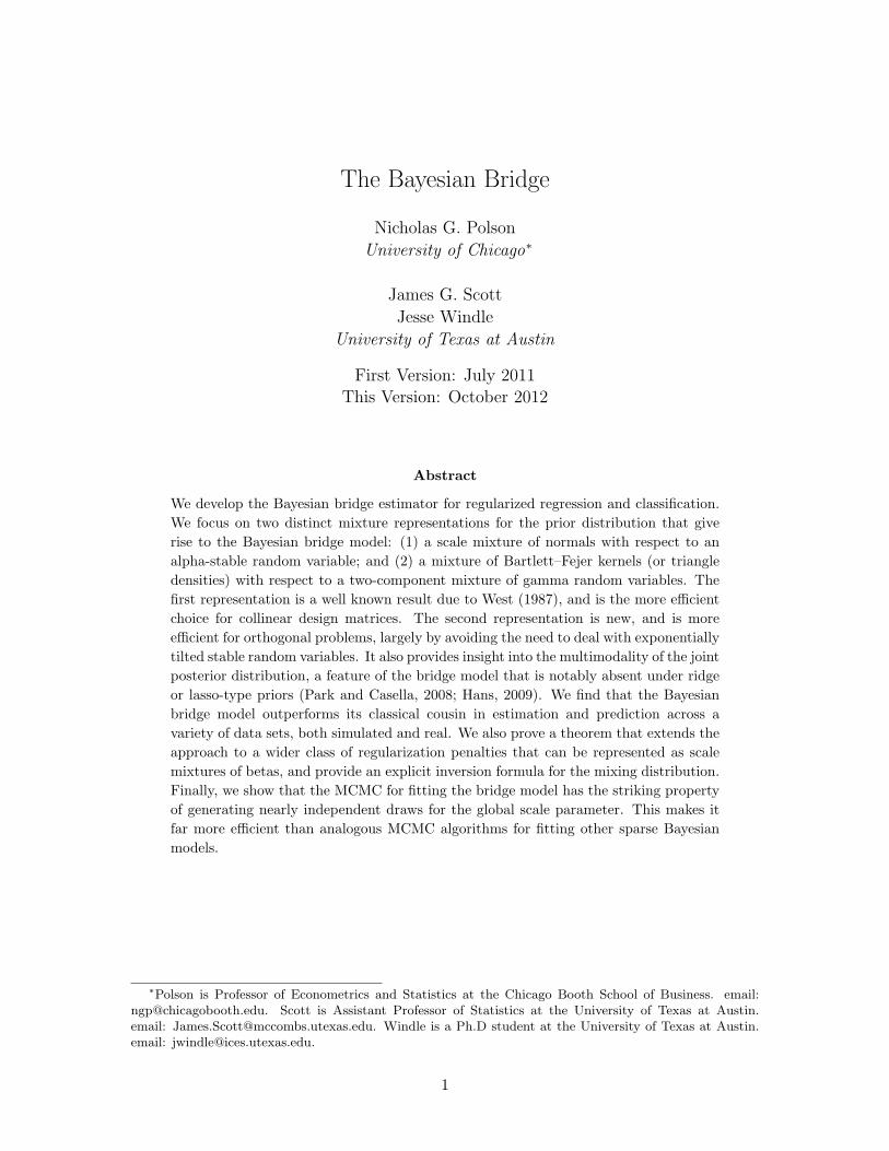
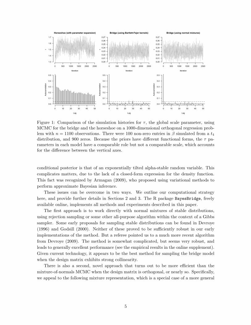
In light of these difficulties, it comes as something of a surprise that the Bayesianbridge model leads to an MCMC strategy with an excellent mixing rate. There are actuallytwo such approaches, both of which have the remarkable property of generating nearlyindependent draws for τ , the global scale parameter. For example, Figure 1 compares theperformance of our bridge MCMC versus the best known Gibbs sampler for fitting thehorseshoe prior (Carvalho et al., 2010) on a 1000-variable orthogonal regression problemwith 900 zero entries in β. (See the supplement for details.) The plots show the first 2500iterations of the sampler, starting from τ = 1. There is a dramatic difference in the effectivesampling rate for τ , which controls the overall level of sparsity in the estimate of β. (Thoughthese results are not shown here, equally striking differences emerge when comparing thesimulation histories of the local scale parameters under each method.)
1.3 Computational approach
Thus we would summarize the potential advantages of the Bayesian bridge as follows. Itleads to richer model summaries, superior performance in estimation and prediction, andbetter uncertainty quantification compared to the classical bridge. It is better at handlingsparsity than the Bayesian lasso. And it leads to an MCMC with superior mixing comparedto other heavy-tailed, sparsity-inducing priors widely used in Bayesian inference.
These advantages, however, do not come for free. In particular, posterior inference forthe Bayesian bridge is more challenging than in most other Bayesian models of this type,where MCMC sampling relies upon representing the implied prior distribution for βj as ascale mixture of normals. The exponential-power prior in (2) is known to lie within thenormal-scale mixture class (West, 1987). Yet the mixing distribution that arises in the
4
0 500 1000 1500 2000 2500
1.3
1.4
1.5
1.6
1.7
Horseshoe (with parameter expansion)
Iteration
τ
0 500 1000 1500 2000 2500
0.20
0.21
0.22
0.23
0.24
0.25
0.26
0.27
Bridge (using Bartlett-Fejer kernels)
Iteration
τ
0 500 1000 1500 2000 2500
0.20
0.21
0.22
0.23
0.24
0.25
0.26
0.27
Bridge (using normal mixtures)
Iteration
τ
0 10 20 30 40 50
0.0
0.1
0.2
0.3
0.4
0.5
Lag
Autocorrelation
0 10 20 30 40 50
0.0
0.1
0.2
0.3
0.4
0.5
Lag
Autocorrelation
0 10 20 30 40 50
0.0
0.1
0.2
0.3
0.4
0.5
Lag
Autocorrelation
Figure 1: Comparison of the simulation histories for τ , the global scale parameter, usingMCMC for the bridge and the horseshoe on a 1000-dimensional orthogonal regression prob-lem with n = 1100 observations. There were 100 non-zero entries in β simulated from a t4distribution, and 900 zeros. Because the priors have different functional forms, the τ pa-rameters in each model have a comparable role but not a comparable scale, which accountsfor the difference between the vertical axes.
conditional posterior is that of an exponentially tilted alpha-stable random variable. Thiscomplicates matters, due to the lack of a closed-form expression for the density function.This fact was recognized by Armagan (2009), who proposed using variational methods toperform approximate Bayesian inference.
These issues can be overcome in two ways. We outline our computational strategyhere, and provide further details in Sections 2 and 3. The R package BayesBridge, freelyavailable online, implements all methods and experiments described in this paper.
The first approach is to work directly with normal mixtures of stable distributions,using rejection sampling or some other all-purpose algorithm within the context of a Gibbssampler. Some early proposals for sampling stable distributions can be found in Devroye(1996) and Godsill (2000). Neither of these proved to be sufficiently robust in our earlyimplementations of the method. But a referee pointed us to a much more recent algorithmfrom Devroye (2009). The method is somewhat complicated, but seems very robust, andleads to generally excellent performance (see the empirical results in the online supplement).Given current technology, it appears to be the best method for sampling the bridge modelwhen the design matrix exhibits strong collinearity.
There is also a second, novel approach that turns out to be more efficient than themixture-of-normals MCMC when the design matrix is orthogonal, or nearly so. Specifically,we appeal to the following mixture representation, which is a special case of a more general
5
−10 −5 0 5 10
0.0
0.2
0.4
0.6
0.8
1.0
Normalized Bartlett kernels (alpha=0.5)
Beta
omega=1.0omega=1.5omega=3.0
0 2 4 6 8 10
0.00
0.05
0.10
0.15
0.20
0.25
The mixing distribution for omega
Omega
Den
sity
alpha=0.75alpha=0.25
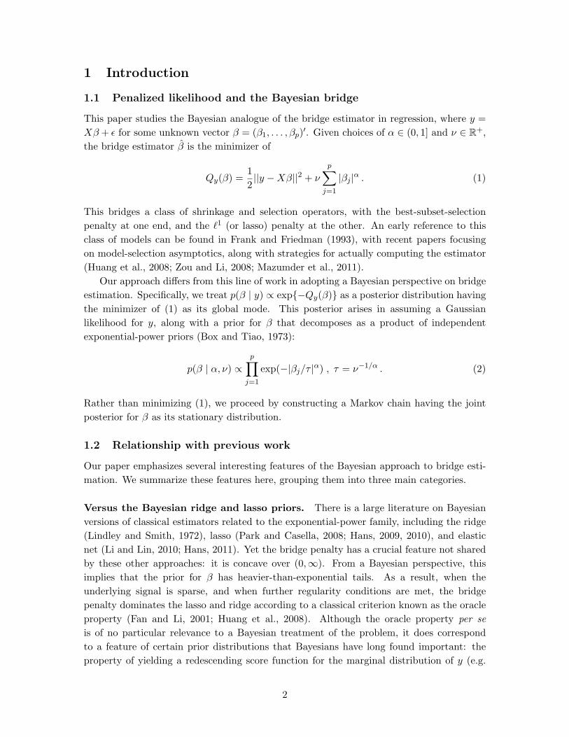
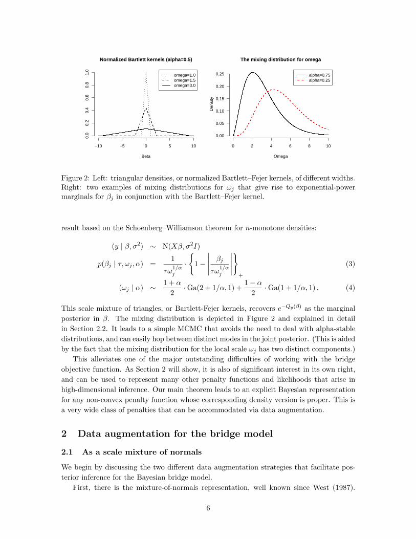
Figure 2: Left: triangular densities, or normalized Bartlett–Fejer kernels, of different widths.Right: two examples of mixing distributions for ωj that give rise to exponential-powermarginals for βj in conjunction with the Bartlett–Fejer kernel.
result based on the Schoenberg–Williamson theorem for n-monotone densities:
(y | β, σ2) ∼ N(Xβ, σ2I)
p(βj | τ, ωj , α) =1
τω1/αj
·
1−
∣∣∣∣∣ βj
τω1/αj
∣∣∣∣∣
+
(3)
(ωj | α) ∼ 1 + α
2·Ga(2 + 1/α, 1) +
1− α2·Ga(1 + 1/α, 1) . (4)
This scale mixture of triangles, or Bartlett-Fejer kernels, recovers e−Qy(β) as the marginalposterior in β. The mixing distribution is depicted in Figure 2 and explained in detailin Section 2.2. It leads to a simple MCMC that avoids the need to deal with alpha-stabledistributions, and can easily hop between distinct modes in the joint posterior. (This is aidedby the fact that the mixing distribution for the local scale ωj has two distinct components.)
This alleviates one of the major outstanding difficulties of working with the bridgeobjective function. As Section 2 will show, it is also of significant interest in its own right,and can be used to represent many other penalty functions and likelihoods that arise inhigh-dimensional inference. Our main theorem leads to an explicit Bayesian representationfor any non-convex penalty function whose corresponding density version is proper. This isa very wide class of penalties that can be accommodated via data augmentation.
2 Data augmentation for the bridge model
2.1 As a scale mixture of normals
We begin by discussing the two different data augmentation strategies that facilitate pos-terior inference for the Bayesian bridge model.
First, there is the mixture-of-normals representation, well known since West (1987).
6
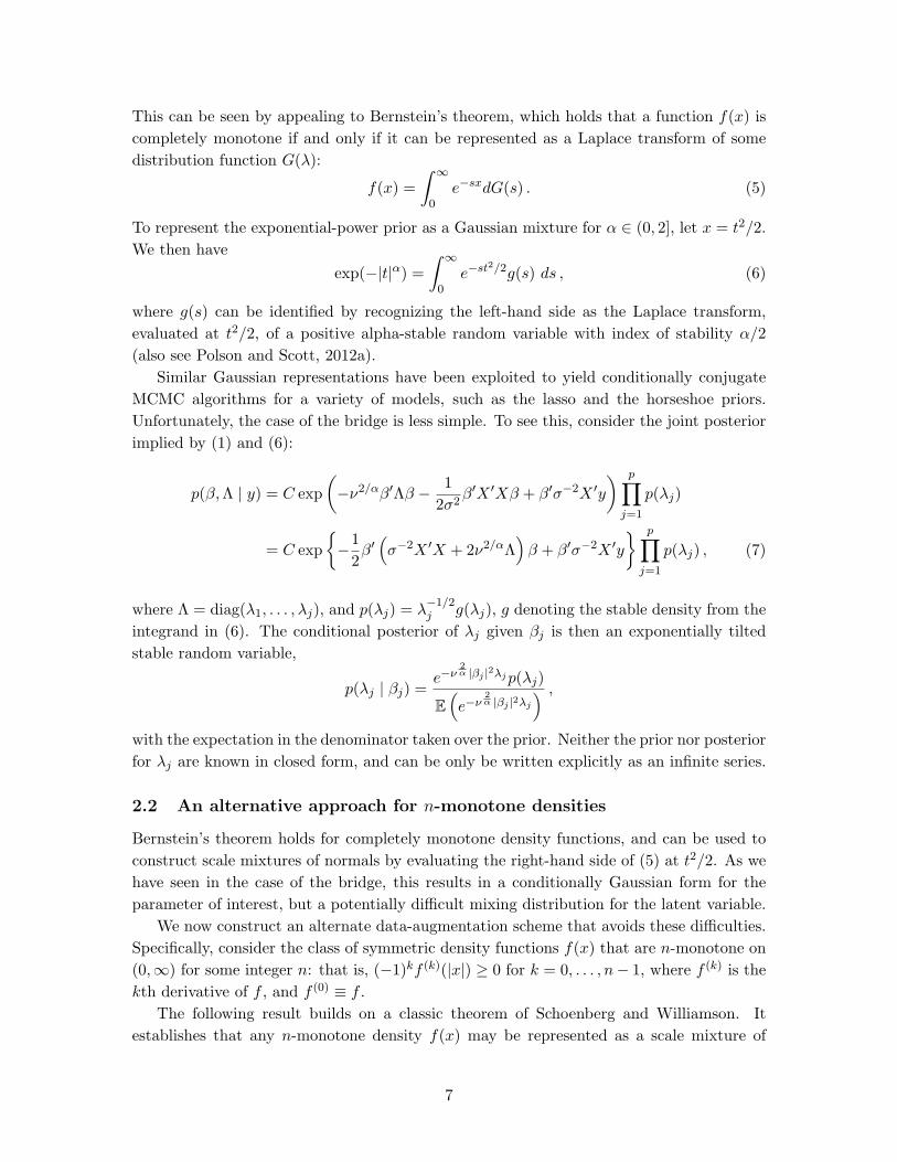
This can be seen by appealing to Bernstein’s theorem, which holds that a function f(x) iscompletely monotone if and only if it can be represented as a Laplace transform of somedistribution function G(λ):
f(x) =∫ ∞
0e−sxdG(s) . (5)
To represent the exponential-power prior as a Gaussian mixture for α ∈ (0, 2], let x = t2/2.We then have
exp(−|t|α) =∫ ∞
0e−st
2/2g(s) ds , (6)
where g(s) can be identified by recognizing the left-hand side as the Laplace transform,evaluated at t2/2, of a positive alpha-stable random variable with index of stability α/2(also see Polson and Scott, 2012a).
Similar Gaussian representations have been exploited to yield conditionally conjugateMCMC algorithms for a variety of models, such as the lasso and the horseshoe priors.Unfortunately, the case of the bridge is less simple. To see this, consider the joint posteriorimplied by (1) and (6):
p(β,Λ | y) = C exp(−ν2/αβ′Λβ − 1
2σ2β′X ′Xβ + β′σ−2X ′y
) p∏j=1
p(λj)
= C exp−1
2β′(σ−2X ′X + 2ν2/αΛ
)β + β′σ−2X ′y
p∏j=1
p(λj) , (7)
where Λ = diag(λ1, . . . , λj), and p(λj) = λ−1/2j g(λj), g denoting the stable density from the
integrand in (6). The conditional posterior of λj given βj is then an exponentially tiltedstable random variable,
p(λj | βj) =e−ν
2α |βj |2λjp(λj)
E(e−ν
2α |βj |2λj
) ,with the expectation in the denominator taken over the prior. Neither the prior nor posteriorfor λj are known in closed form, and can be only be written explicitly as an infinite series.
2.2 An alternative approach for n-monotone densities
Bernstein’s theorem holds for completely monotone density functions, and can be used toconstruct scale mixtures of normals by evaluating the right-hand side of (5) at t2/2. As wehave seen in the case of the bridge, this results in a conditionally Gaussian form for theparameter of interest, but a potentially difficult mixing distribution for the latent variable.
We now construct an alternate data-augmentation scheme that avoids these difficulties.Specifically, consider the class of symmetric density functions f(x) that are n-monotone on(0,∞) for some integer n: that is, (−1)kf (k)(|x|) ≥ 0 for k = 0, . . . , n− 1, where f (k) is thekth derivative of f , and f (0) ≡ f .
The following result builds on a classic theorem of Schoenberg and Williamson. Itestablishes that any n-monotone density f(x) may be represented as a scale mixture of
7
betas, and that we may invert for the mixing distribution using the derivatives of f .
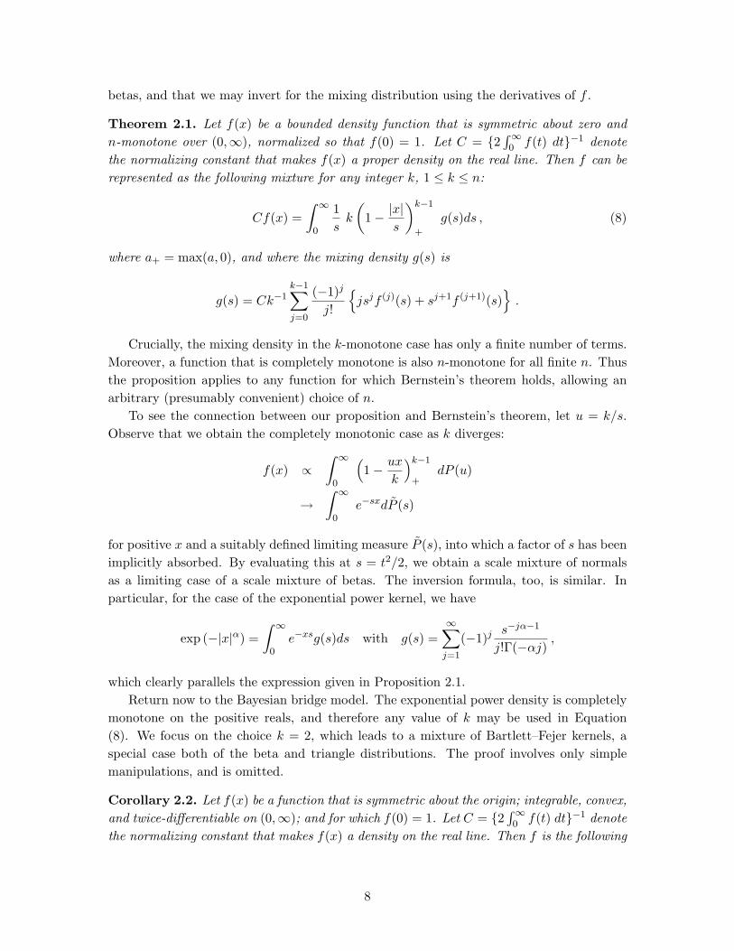
Theorem 2.1. Let f(x) be a bounded density function that is symmetric about zero andn-monotone over (0,∞), normalized so that f(0) = 1. Let C = 2
∫∞0 f(t) dt−1 denote
the normalizing constant that makes f(x) a proper density on the real line. Then f can berepresented as the following mixture for any integer k, 1 ≤ k ≤ n:
Cf(x) =∫ ∞
0
1sk
(1− |x|
s
)k−1
+
g(s)ds , (8)
where a+ = max(a, 0), and where the mixing density g(s) is
g(s) = Ck−1k−1∑j=0
(−1)j
j!
jsjf (j)(s) + sj+1f (j+1)(s)
.
Crucially, the mixing density in the k-monotone case has only a finite number of terms.Moreover, a function that is completely monotone is also n-monotone for all finite n. Thusthe proposition applies to any function for which Bernstein’s theorem holds, allowing anarbitrary (presumably convenient) choice of n.
To see the connection between our proposition and Bernstein’s theorem, let u = k/s.Observe that we obtain the completely monotonic case as k diverges:
f(x) ∝∫ ∞
0
(1− ux
k
)k−1
+dP (u)
→∫ ∞
0e−sxdP (s)
for positive x and a suitably defined limiting measure P (s), into which a factor of s has beenimplicitly absorbed. By evaluating this at s = t2/2, we obtain a scale mixture of normalsas a limiting case of a scale mixture of betas. The inversion formula, too, is similar. Inparticular, for the case of the exponential power kernel, we have
exp (−|x|α) =∫ ∞
0e−xsg(s)ds with g(s) =
∞∑j=1
(−1)js−jα−1
j!Γ(−αj),
which clearly parallels the expression given in Proposition 2.1.Return now to the Bayesian bridge model. The exponential power density is completely
monotone on the positive reals, and therefore any value of k may be used in Equation(8). We focus on the choice k = 2, which leads to a mixture of Bartlett–Fejer kernels, aspecial case both of the beta and triangle distributions. The proof involves only simplemanipulations, and is omitted.
Corollary 2.2. Let f(x) be a function that is symmetric about the origin; integrable, convex,and twice-differentiable on (0,∞); and for which f(0) = 1. Let C = 2
∫∞0 f(t) dt−1 denote
the normalizing constant that makes f(x) a density on the real line. Then f is the following
8
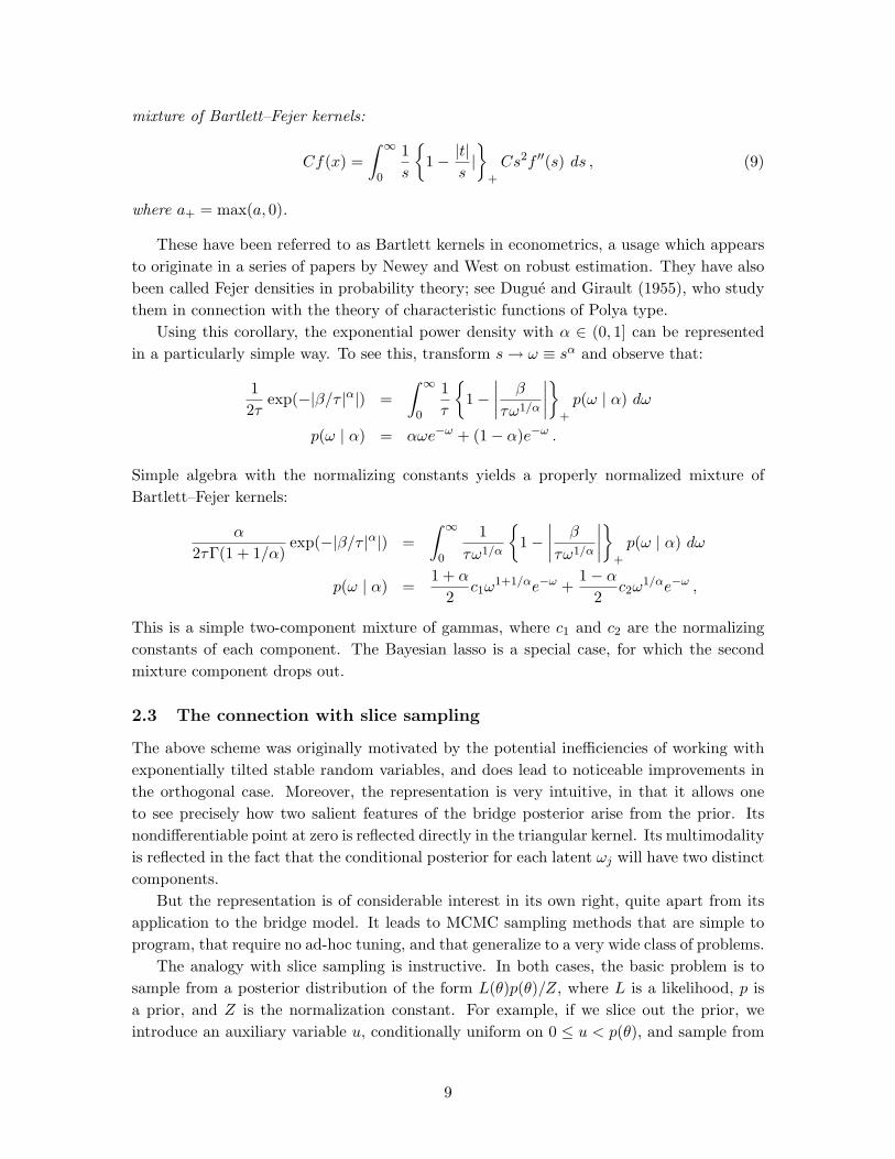
mixture of Bartlett–Fejer kernels:
Cf(x) =∫ ∞
0
1s
1− |t|
s|
+
Cs2f ′′(s) ds , (9)
where a+ = max(a, 0).
These have been referred to as Bartlett kernels in econometrics, a usage which appearsto originate in a series of papers by Newey and West on robust estimation. They have alsobeen called Fejer densities in probability theory; see Dugue and Girault (1955), who studythem in connection with the theory of characteristic functions of Polya type.
Using this corollary, the exponential power density with α ∈ (0, 1] can be representedin a particularly simple way. To see this, transform s→ ω ≡ sα and observe that:
12τ
exp(−|β/τ |α|) =∫ ∞
0
1τ
1−
∣∣∣∣ β
τω1/α
∣∣∣∣+
p(ω | α) dω
p(ω | α) = αωe−ω + (1− α)e−ω .
Simple algebra with the normalizing constants yields a properly normalized mixture ofBartlett–Fejer kernels:
α
2τΓ(1 + 1/α)exp(−|β/τ |α|) =
∫ ∞0
1τω1/α
1−
∣∣∣∣ β
τω1/α
∣∣∣∣+
p(ω | α) dω
p(ω | α) =1 + α
2c1ω
1+1/αe−ω +1− α
2c2ω
1/αe−ω ,
This is a simple two-component mixture of gammas, where c1 and c2 are the normalizingconstants of each component. The Bayesian lasso is a special case, for which the secondmixture component drops out.
2.3 The connection with slice sampling
The above scheme was originally motivated by the potential inefficiencies of working withexponentially tilted stable random variables, and does lead to noticeable improvements inthe orthogonal case. Moreover, the representation is very intuitive, in that it allows oneto see precisely how two salient features of the bridge posterior arise from the prior. Itsnondifferentiable point at zero is reflected directly in the triangular kernel. Its multimodalityis reflected in the fact that the conditional posterior for each latent ωj will have two distinctcomponents.
But the representation is of considerable interest in its own right, quite apart from itsapplication to the bridge model. It leads to MCMC sampling methods that are simple toprogram, that require no ad-hoc tuning, and that generalize to a very wide class of problems.
The analogy with slice sampling is instructive. In both cases, the basic problem is tosample from a posterior distribution of the form L(θ)p(θ)/Z, where L is a likelihood, p isa prior, and Z is the normalization constant. For example, if we slice out the prior, weintroduce an auxiliary variable u, conditionally uniform on 0 ≤ u < p(θ), and sample from
9
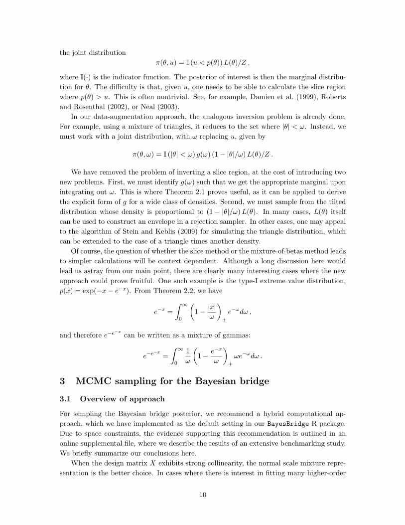
the joint distributionπ(θ, u) = I (u < p(θ))L(θ)/Z ,
where I(·) is the indicator function. The posterior of interest is then the marginal distribu-tion for θ. The difficulty is that, given u, one needs to be able to calculate the slice regionwhere p(θ) > u. This is often nontrivial. See, for example, Damien et al. (1999), Robertsand Rosenthal (2002), or Neal (2003).
In our data-augmentation approach, the analogous inversion problem is already done.For example, using a mixture of triangles, it reduces to the set where |θ| < ω. Instead, wemust work with a joint distribution, with ω replacing u, given by
π(θ, ω) = I (|θ| < ω) g(ω) (1− |θ|/ω)L(θ)/Z .
We have removed the problem of inverting a slice region, at the cost of introducing twonew problems. First, we must identify g(ω) such that we get the appropriate marginal uponintegrating out ω. This is where Theorem 2.1 proves useful, as it can be applied to derivethe explicit form of g for a wide class of densities. Second, we must sample from the tilteddistribution whose density is proportional to (1− |θ|/ω)L(θ). In many cases, L(θ) itselfcan be used to construct an envelope in a rejection sampler. In other cases, one may appealto the algorithm of Stein and Keblis (2009) for simulating the triangle distribution, whichcan be extended to the case of a triangle times another density.
Of course, the question of whether the slice method or the mixture-of-betas method leadsto simpler calculations will be context dependent. Although a long discussion here wouldlead us astray from our main point, there are clearly many interesting cases where the newapproach could prove fruitful. One such example is the type-I extreme value distribution,p(x) = exp(−x− e−x). From Theorem 2.2, we have
e−x =∫ ∞
0
(1− |x|
ω
)+
e−ωdω ,
and therefore e−e−x
can be written as a mixture of gammas:
e−e−x
=∫ ∞
0
1ω
(1− e−x
ω
)+
ωe−ωdω .
3 MCMC sampling for the Bayesian bridge
3.1 Overview of approach
For sampling the Bayesian bridge posterior, we recommend a hybrid computational ap-proach, which we have implemented as the default setting in our BayesBridge R package.Due to space constraints, the evidence supporting this recommendation is outlined in anonline supplemental file, where we describe the results of an extensive benchmarking study.We briefly summarize our conclusions here.
When the design matrix X exhibits strong collinearity, the normal scale mixture repre-sentation is the better choice. In cases where there is interest in fitting many higher-order
10
interaction terms, the efficiency advantage can be substantial. On the other hand, theBartlett-Fejer representation is the better choice when the design matrix is orthogonal,usually enjoying an effective sampling rate roughly two to three times that of the Gaussianmethod. The orthogonal case applies to nonlinear regression problems where the effect of acovariate is expanded in an orthogonal basis. It also has connections with the generalizedg-priors for p > n problems discussed in Polson and Scott (2012a).
Once one has a method for sampling exponentially tilted alpha-stable random variables,it is easy to use (7) to generate posterior draws, appealing to standard multivariate normaltheory. Thus we omit a discussion of this method in the main manuscript, and focus on themixture-of-betas approach.
3.2 Sampling β and the latent variables
To see why the representation in (3)–(4) leads to a simple algorithm for posterior sampling,consider the joint distribution for β and the latent ωj ’s:
p(β,Ω | τ, y) = C exp(− 1
2σ2β′X ′Xβ +
1σ2β′X ′y
) p∏i=1
p(ωj | α)p∏i=1
(1− |βj |
τω1/αj
)+
. (10)
Introduce further slice variables u1, . . . , uj . This leads to the joint posterior
p(β,Ω, u | τ, y) ∝ exp(− 1
2σ2β′X ′Xβ +
1σ2β′X ′y
)×
p∏j=1
p(ωj | α)p∏j=1
I
(0 ≤ uj ≤ 1− |βj |
τω1/αj
). (11)
Note that we have implicitly absorbed a factor of ω1/α from the normalization constant forthe Bartlett–Fejer kernel into the gamma conditional for ωj . This will make inverting theslice region for ωj far easier.
Applying Corollary 2.2, if we marginalize out both the slice variables and the latentωj ’s, we recover the Bayesian bridge posterior distribution,
p(β | y) = C exp
− 12σ2‖y −Xβ‖2 −
p∑j=1
|βj/τ |α .
We can invert the slice region in (11) by defining (aj , bj) as
|βj | ≤ τ−1(1− uj)ω1/αj = bj and ωj ≥
(τ |βj |
1− uj
)α= aj .
This leads us to an exact Gibbs sampler that starts at initial guesses for (β,Ω) and iteratesthe following steps:
1. Generate (uj | βj , ωj) ∼ Unif(
0, 1− τ |βj |ω−1/αj
).
2. Generate each ωj from a mixture of truncated gammas, as described below.
11
3. Generate β from a truncated multivariate normal proportional to
N(β, σ2(X ′X)−1
)I (|βj | ≤ bj for all j) ,
where β indicates the least-squares estimate for β.
We explored several different methods for simulating from the truncated multivariatenormal, ultimately settling on the proposal of Rodriguez-Yam et al. (2004) as the most effi-cient. The conditional posterior of the latent ωj ’s can be determined as follows. Suppressingsubscripts for the moment, it is clear from (11) that
p(ω | α) = α(ωe−ω) + (1− α)e−ω
p(ω | a, α) = Caα(ωe−ω) + (1− α)e−ω
I (ω ≥ a) ,
where a comes from inverting the slice region in (11) and Ca is the normalization constant.We can simulate from this mixture of truncated gammas by defining ω = ω − a, where
ω > 0. Then ω has density
p(ω|a, α) = Caαe−a(a+ ω)e−ω + (1− α)e−ae−ω
=
α
1 + αa· ωe−ω +
1− α(1 + a)1 + αa
· e−ω .
This is a mixture of gammas, where
(ω | a) ∼
Γ(1, 1) with prob 1−α(1+a)
1+αa
Γ(2, 1) with prob α1+αa .
After sampling ω, simply transform back using the fact that ω = a+ ω.This representation has two interesting and intuitive features. First, full conditional for
β in step 3 is centered at the usual least-squares estimate β. Only the truncations (bj)change at each step, which speeds matrix operations. Compare this to the usual scale-mixture representation, which involves inverting a matrix of the form (X ′X+Λ)−1 at everyMCMC step.
Second, the mixture-of-gammas form of p(ω) naturally accounts for the bimodality inthe marginal posterior distribution, p(βj | y) =
∫p(βj | ω, y)p(ωj | y)dωj . Each mixture
component of the conditional for ωj represents a distinct mode of the marginal posterior forβj . As the examples later will show, this endows the algorithm with the ability to explorevarious modes of the joint posterior very easily.
3.3 Sampling hyperparameters
To update the global scale parameter τ , we work directly with the exponential-power density,marginalizing out the latent variables ωj , uj. From (1), observe that the posterior for
12
ν ≡ τ−α, given β, is conditionally independent of y, and takes the form
p(ν | β) ∝ νp/α exp(−νp∑j=1
|βj |α) p(ν) .
Therefore if ν has a Gamma(c, d) prior, its conditional posterior will also be a gamma dis-tribution, with hyperparameters c? = c+p/α and d? = d+
∑pj=1 |βj |α. To sample τ , simply
draw ν from this gamma distribution, and use the transformation τ = ν−1/α. Alterna-tive priors for ν can also be considered, in which case the gamma form of the conditionallikelihood in ν will make for a useful proposal distribution that closely approximates theposterior. As Figure 1 from the introduction shows, the ability to marginalize over the localscales in sampling τ is crucial here in leading to a good mixing rate.
In many cases the concavity parameter α will be fixed ahead of time to reflect a particulardesired shape of the penalty function. But it too can be give a prior p(α), most convenientlyfrom the beta family, and can be updated using a random-walk Metropolis sampler.
4 Examples
4.1 Diabetes data
We first explore the Bayesian bridge estimator using the well-known data set on diabetesamong Pima Indians, available in the R package lars (see, e.g. Efron et al., 2004). The maindata set has 10 predictors and 442 observations. Yet even for this relatively information-richproblem, significant differences emerge between the Bayesian and classical methods.
We also fit the Bayesian bridge, using Algorithm 1 and a default Gamma(2,2) prior forν. We also fit the classical bridge, using generalized cross validation and the EM algorithmfrom Polson and Scott (2011b). Both the predictor and responses were centered, while thepredictors were also re-scaled to have unit variance. At each step of the MCMC for theBayesian model, we calculated the conditional posterior density for each βj at a discretegrid of values.
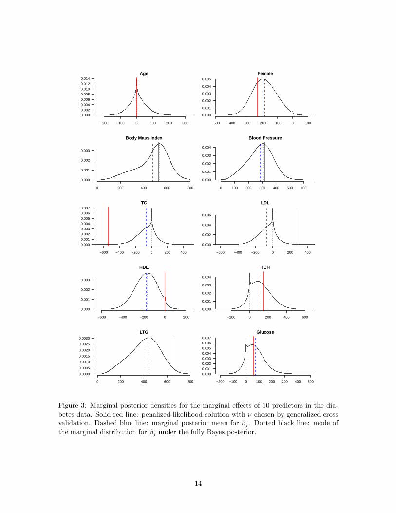
Figure 3 summarizes the results of the two fits, showing both the marginal posterior den-sity and the classical bridge solution for each of the 10 regression coefficients. One notablefeature of the problem is the pronounced multimodality in the joint posterior distributionfor the Bayesian bridge. Observe, for example, the two distinct modes in the marginalposteriors for the coefficients associated with the TCH and Glucose predictors (and, to alesser extent, for the HDL and Female predictors). In none of these cases does it seemsatisfactory to summarize information about βj using only a single number, as the classicalsolution forces one to do.
Second, observe that the classical bridge solution does not coincide with the joint mode ofthe fully Bayesian posterior distribution. This discrepancy can be attributed to uncertaintyin τ and σ, which is ignored in the classical solution. Marginalizing over these hyperparam-eters leads to a fundamentally different objective function, and therefore a different jointposterior mode.
The difference between the classical mode and the Bayesian mode, moreover, need not
13
Age
−200 −100 0 100 200 300
0.000
0.002
0.004
0.006
0.008
0.010
0.012
0.014Female
−500 −400 −300 −200 −100 0 100
0.000
0.001
0.002
0.003
0.004
0.005
Body Mass Index
0 200 400 600 800
0.000
0.001
0.002
0.003
Blood Pressure
0 100 200 300 400 500 600
0.000
0.001
0.002
0.003
0.004
TC
−600 −400 −200 0 200 400
0.000
0.001
0.002
0.003
0.004
0.005
0.006
0.007LDL
−600 −400 −200 0 200 400
0.000
0.002
0.004
0.006
HDL
−600 −400 −200 0 200
0.000
0.001
0.002
0.003
TCH
−200 0 200 400 600
0.000
0.001
0.002
0.003
0.004
LTG
0 200 400 600 800
0.0000
0.0005
0.0010
0.0015
0.0020
0.0025
0.0030
Glucose
−200 −100 0 100 200 300 400 500
0.0000.0010.0020.0030.0040.0050.0060.007
Figure 3: Marginal posterior densities for the marginal effects of 10 predictors in the dia-betes data. Solid red line: penalized-likelihood solution with ν chosen by generalized crossvalidation. Dashed blue line: marginal posterior mean for βj . Dotted black line: mode ofthe marginal distribution for βj under the fully Bayes posterior.
14
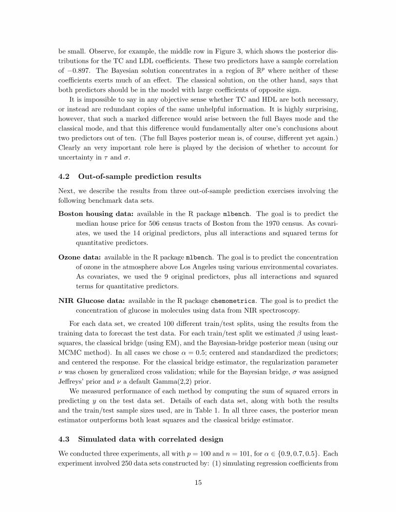
be small. Observe, for example, the middle row in Figure 3, which shows the posterior dis-tributions for the TC and LDL coefficients. These two predictors have a sample correlationof −0.897. The Bayesian solution concentrates in a region of Rp where neither of thesecoefficients exerts much of an effect. The classical solution, on the other hand, says thatboth predictors should be in the model with large coefficients of opposite sign.
It is impossible to say in any objective sense whether TC and HDL are both necessary,or instead are redundant copies of the same unhelpful information. It is highly surprising,however, that such a marked difference would arise between the full Bayes mode and theclassical mode, and that this difference would fundamentally alter one’s conclusions abouttwo predictors out of ten. (The full Bayes posterior mean is, of course, different yet again.)Clearly an very important role here is played by the decision of whether to account foruncertainty in τ and σ.
4.2 Out-of-sample prediction results
Next, we describe the results from three out-of-sample prediction exercises involving thefollowing benchmark data sets.
Boston housing data: available in the R package mlbench. The goal is to predict themedian house price for 506 census tracts of Boston from the 1970 census. As covari-ates, we used the 14 original predictors, plus all interactions and squared terms forquantitative predictors.
Ozone data: available in the R package mlbench. The goal is to predict the concentrationof ozone in the atmosphere above Los Angeles using various environmental covariates.As covariates, we used the 9 original predictors, plus all interactions and squaredterms for quantitative predictors.
NIR Glucose data: available in the R package chemometrics. The goal is to predict theconcentration of glucose in molecules using data from NIR spectroscopy.
For each data set, we created 100 different train/test splits, using the results from thetraining data to forecast the test data. For each train/test split we estimated β using least-squares, the classical bridge (using EM), and the Bayesian-bridge posterior mean (using ourMCMC method). In all cases we chose α = 0.5; centered and standardized the predictors;and centered the response. For the classical bridge estimator, the regularization parameterν was chosen by generalized cross validation; while for the Bayesian bridge, σ was assignedJeffreys’ prior and ν a default Gamma(2,2) prior.
We measured performance of each method by computing the sum of squared errors inpredicting y on the test data set. Details of each data set, along with both the resultsand the train/test sample sizes used, are in Table 1. In all three cases, the posterior meanestimator outperforms both least squares and the classical bridge estimator.
4.3 Simulated data with correlated design
We conducted three experiments, all with p = 100 and n = 101, for α ∈ 0.9, 0.7, 0.5. Eachexperiment involved 250 data sets constructed by: (1) simulating regression coefficients from
15
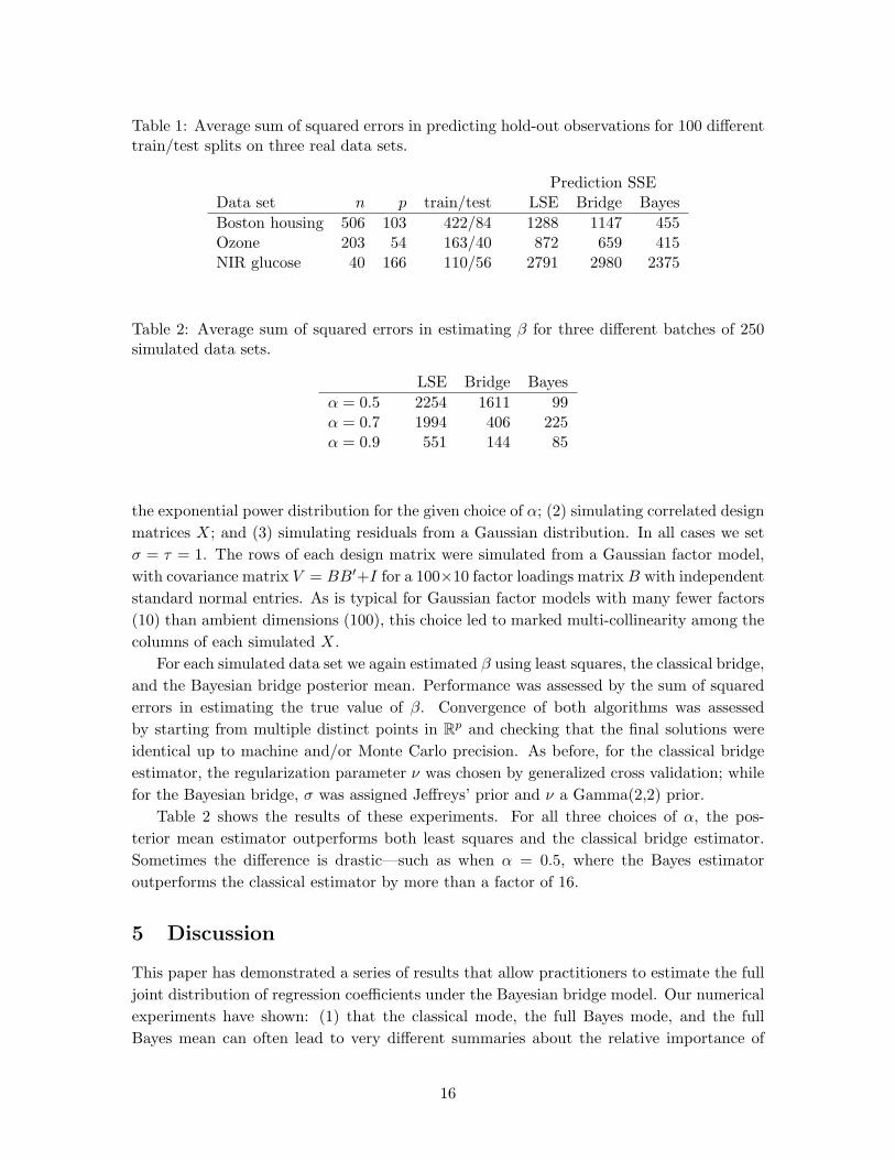
Table 1: Average sum of squared errors in predicting hold-out observations for 100 differenttrain/test splits on three real data sets.
Prediction SSEData set n p train/test LSE Bridge BayesBoston housing 506 103 422/84 1288 1147 455Ozone 203 54 163/40 872 659 415NIR glucose 40 166 110/56 2791 2980 2375
Table 2: Average sum of squared errors in estimating β for three different batches of 250simulated data sets.
LSE Bridge Bayesα = 0.5 2254 1611 99α = 0.7 1994 406 225α = 0.9 551 144 85
the exponential power distribution for the given choice of α; (2) simulating correlated designmatrices X; and (3) simulating residuals from a Gaussian distribution. In all cases we setσ = τ = 1. The rows of each design matrix were simulated from a Gaussian factor model,with covariance matrix V = BB′+I for a 100×10 factor loadings matrix B with independentstandard normal entries. As is typical for Gaussian factor models with many fewer factors(10) than ambient dimensions (100), this choice led to marked multi-collinearity among thecolumns of each simulated X.
For each simulated data set we again estimated β using least squares, the classical bridge,and the Bayesian bridge posterior mean. Performance was assessed by the sum of squarederrors in estimating the true value of β. Convergence of both algorithms was assessedby starting from multiple distinct points in Rp and checking that the final solutions wereidentical up to machine and/or Monte Carlo precision. As before, for the classical bridgeestimator, the regularization parameter ν was chosen by generalized cross validation; whilefor the Bayesian bridge, σ was assigned Jeffreys’ prior and ν a Gamma(2,2) prior.
Table 2 shows the results of these experiments. For all three choices of α, the pos-terior mean estimator outperforms both least squares and the classical bridge estimator.Sometimes the difference is drastic—such as when α = 0.5, where the Bayes estimatoroutperforms the classical estimator by more than a factor of 16.
5 Discussion
This paper has demonstrated a series of results that allow practitioners to estimate the fulljoint distribution of regression coefficients under the Bayesian bridge model. Our numericalexperiments have shown: (1) that the classical mode, the full Bayes mode, and the fullBayes mean can often lead to very different summaries about the relative importance of
16
different predictors; and (2) that using the posterior mean offers substantial improvementsover the mode when estimating β or making predictions under squared-error loss. Bothresults parallel the findings of Park and Casella (2008) and Hans (2009) for the Bayesianlasso.
The existence of a second, novel mixture representation for the Bayesian bridge is ofparticular interest, and suggests many generalizations, some of which we have mentioned.Our main theorem leads to a novel Gibbs-sampling scheme for the bridge that—by virtue ofworking directly with a two-component mixing measure for each latent scale ωj—is capableof easily jumping between modes in the joint posterior distribution. It thereby avoids manyof the difficulties associated with slow mixing in global-local scale-mixture models describedby Hans (2009), and further studied in the online supplemental file. It appears to be thebest algorithm in the orthogonal case, but suffers from poor mixing when the design matrixis extremely collinear. Luckily, in this case, the normal-mixture method based on the workof Devroye (2009) for sampling exponentially tilted stable random variables performs well.Both methods are implemented in the R package BayesBridge, available through CRAN.Together, they give practioners a set of tools for efficiently exploring the bridge model acrossa wide range of commonly encountered situations.
A Proofs
A.1 Theorem 2.1
Proof. Let Mn denote the class of n-times monotone functions on (0,∞). Clearly for n ≥ 2,f ∈ Mn ⇒ f ∈ Mn−1. Thus it is sufficient to prove the proposition for k = n. As thedensity f(x) is symmetric, we consider only positive values of x.
The Schoenberg–Williamson theorem (Williamson, 1956) states that a necessary andsufficient condition for a function f(x) defined on (0,∞) to be in Mn is that
f(x) =∫ ∞
0(1− ut)n−1
+ dG(u) ,
for some G(u) that is non-decreasing and bounded below. Moreover, if G(u) = 0, therepresentation is unique, in the sense of being determined at the points of continuity ofG(u), and is given by
G(u) =n−1∑j=0
(−1)jf (j)(1/u)j!
(1u
)j.
References
A. Armagan. Variational bridge regression. Journal of Machine Learning Research W&CP, 5(17–24), 2009.
A. Armagan, D. Dunson, and J. Lee. Generalized double Pareto shrinkage. Statistica Sinica, to appear,2012.
17
K. Bae and B. Mallick. Gene selection using a two-level hierarchical Bayesian model. Bioinformatics, 20(18):3423–30, 2004.
G. Box and G. C. Tiao. Bayesian Inference in Statistical Analysis. Addison-Wesley, 1973.
F. Caron and A. Doucet. Sparse Bayesian nonparametric regression. In Proceedings of the 25th InternationalConference on Machine Learning, pages 88–95. Association for Computing Machinery, Helsinki, Finland,2008.
C. M. Carvalho, N. G. Polson, and J. G. Scott. The horseshoe estimator for sparse signals. Biometrika, 97(2):465–80, 2010.
P. Damien, J. C. Wakefield, and S. G. Walker. Bayesian nonconjugate and hierarchical models by usingauxiliary variables. J. R. Stat. Soc. Ser. B, Stat. Methodol., 61:331–44, 1999.
L. Devroye. Random variate generation in one line of code. In J. Charnes, D. Morrice, D. Brunner, andJ. Swain, editors, Proceedings of the 1996 Winter Simulation Conference, pages 265–72, 1996.
L. Devroye. On exact simulation algorithms for some distributions related to Jacobi theta functions. Statistics& Probability Letters, 79(21):2251–9, 2009.
D. Dugue and M. Girault. Fonctions convexes de Polya. Publications de l’Institut de Statistique des Univer-sites de Paris, 4:3–10, 1955.
B. Efron. Empirical Bayes estimates for large-scale prediction problems. Journal of the American StatisticalAssociation, 104(487):1015–28, 2009.
B. Efron, T. Hastie, I. Johnstone, and R. Tibshirani. Least angle regression. The Annals of Statistics, 32(2):407–99, 2004.
J. Fan and R. Li. Variable selection via nonconcave penalized likelihood and its oracle properties. Journalof the American Statistical Association, 96(456):1348–60, 2001.
M. Figueiredo. Adaptive sparseness for supervised learning. IEEE Transactions on Pattern Analysis andMachine Intelligence, 25(9):1150–9, 2003.
I. Frank and J. H. Friedman. A statistical view of some chemometrics regression tools (with discussion).Technometrics, 35(2):109–135, 1993.
A. Gelman. Prior distributions for variance parameters in hierarchical models. Bayesian Analysis, 1(3):515–33, 2006.
S. Godsill. Inference in symmetric alpha-stable noise using MCMC and the slice sampler. In Acoustics,Speech, and Signal Processing, volume 6, pages 3806–9, 2000.
J. Griffin and P. Brown. Inference with normal-gamma prior distributions in regression problems. BayesianAnalysis, 5(1):171–88, 2010.
J. Griffin and P. Brown. Alternative prior distributions for variable selection with very many more variablesthan observations. Australian and New Zealand Journal of Statistics, 2012. (to appear).
C. M. Hans. Bayesian lasso regression. Biometrika, 96(4):835–45, 2009.
C. M. Hans. Model uncertainty and variable selection in Bayesian lasso regression. Statistics and Computing,20:221–9, 2010.
C. M. Hans. Elastic net regression modeling with the orthant normal prior. Journal of the AmericanStatistical Association, to appear, 2011.
J. Huang, J. Horowitz, and S. Ma. Asymptotic properties of bridge estimators in sparse high-dimensionalregression models. The Annals of Statistics, 36(2):587–613, 2008.
Q. Li and N. Lin. The Bayesian elastic net. Bayesian Analysis, 5(1):151–70, 2010.
18

D. Lindley and A. Smith. Bayes estimates for the linear model. Journal of the Royal Statistical Society,Series B, 34(1–41), 1972.
R. Mazumder, J. Friedman, and T. Hastie. Sparsenet: coordinate descent with non-convex penalties. Journalof the American Statistical Association, 106(495):1125–38, 2011.
R. M. Neal. Slice sampling. The Annals of Statistics, 31(3):705–67, 2003.
T. Park and G. Casella. The Bayesian lasso. Journal of the American Statistical Association, 103(482):681–6, 2008.
L. R. Pericchi and A. Smith. Exact and approximate posterior moments for a normal location parameter.Journal of the Royal Statistical Society (Series B), 54(3):793–804, 1992.
N. G. Polson and J. G. Scott. Shrink globally, act locally: sparse Bayesian regularization and prediction(with discussion). In J. M. Bernardo, M. J. Bayarri, J. O. Berger, A. P. Dawid, D. Heckerman, A. F. M.Smith, and M. West, editors, Proceedings of the 9th Valencia World Meeting on Bayesian Statistics, pages501–38. Oxford University Press, 2011a.
N. G. Polson and J. G. Scott. Data augmentation for non-Gaussian regression models using variance-meanmixtures. Technical report, University of Texas at Austin, http://arxiv.org/abs/1103.5407v3, 2011b.
N. G. Polson and J. G. Scott. Local shrinkage rules, Levy processes, and regularized regression. Journal ofthe Royal Statistical Society (Series B), 74(2):287–311, 2012a.
N. G. Polson and J. G. Scott. On the half-Cauchy prior for a global scale parameter. Bayesian Analysis,2012b.
G. O. Roberts and J. S. Rosenthal. Convergence of slice sampler Markov chains. Journal of the RoyalStatistical Society (Series B), 61(3):643–60, 2002.
G. Rodriguez-Yam, R. A. Davis, and L. L. Scharf. Efficient gibbs sampling of truncated multivariate normalwith application to constrained linear regression. Columbia, March 2004.
W. E. Stein and M. F. Keblis. A new method to simulate the triangular distribution. Mathematical andComputer Modeling, 49(2009):1143–7, 2009.
M. Tipping. Sparse Bayesian learning and the relevance vector machine. Journal of Machine LearningResearch, 1:211–44, 2001.
M. West. On scale mixtures of normal distributions. Biometrika, 74(3):646–8, 1987.
R. Williamson. Multiply monotone functions and their laplace transforms. Duke Mathematics Journal, 23(189–207), 1956.
H. Zou and R. Li. One-step sparse estimates in nonconcave penalized likelihood models. Annals of Statistics,36(4):1509–33, 2008.
19