Embed Size (px)
Citation preview
Article Draft 2
Government Size and Trade Openness using Bayesian Model Average
Kyriakos Petrou
Department of Economics, University of Cyprus
Abstract:
This paper uses the Bayesian Model Average estimation in order to investigate the relationship between
government size and trade openness taking into account the model uncertainty. The empirical findings are
consistent with the efficiency hypothesis. We use three different government size variables and more than
140 dependent variables. In addition, we divide trade openness into two groups. The trade openness under
trade agreement regime, such as Customs Union, Economic Integration Agreement, Free Trade Agreement
and Partial Scope Agreement and the trade openness under no trade agreement regime. We find evidence
against any effect of trade openness under trade agreement regime on government expenditure and a
negative effect of the trade openness under no trade agreement regime on government expenditure, which
supports the efficiency hypothesis.
Keywords: BMA; Government Consumption; Government Expenditure; Trade Agreements; Trade Openness
JEL classification: C11; C26; F13; F15; H5; H7; H87
1
1. Introduction
In the last few years, fiscal adjustment and government expenditure are a part the daily agenda. If we
observe the data about government size we can see that the per year average time trend of government size
increases in time, up to 1989, a year in which we have radical changes in the global scene, then they slightly
decrease up to 2008 and then we have a rapid increase. Since we are in a globalized world the primary
objective of the article is to find the relationship between government size and trade, especially in the case
where trade can be divided into trade agreement regime, such as Customs Union (CU), Economic
Integration Agreement (EIA), Free Trade Agreement (FTA) and Partial Scope Agreement (PSA). From the
data we can see that all types of trade agreements increase from 1958 onwards. This increase though is
sharper after 1989. Also a main objective is to find all possible determinants of government size.
There is a large existing literature about the relationship between government size and trade openness. This
relationship is not clear, but we can divide the literature into two “schools”. Garrett (1995), Schulze and
Ursprung (1999), Garrett (2001) and Garrett and Mitchell (2001) state that under the compensate hypothesis
as a response to globalization the policy makers increases government expenditure. Globalization may well
benefit all segments of society in the long run through the more efficient allocation of production and
investment. The short-term political effects of globalization though are likely to be very different.
Expanding the scope of markets can be expected to have two effects, the increase of inequality and the
increase of economic insecurity which would increase government spending for the support of citizens.
Globalization tends to increase economic inequality, economic insecurity and external risk. From the
demand side of the political market this creates incentives for government to compensate the losers from
globalization, mainly through income transfer programs and economic policy activism. Under the efficiency
hypothesis as a response to globalization the policy makers decrease government expenditure. Government
spending reduces the competitiveness of national producers in international goods and services markets.
Income transfer programs and social services distort labor markets and bias intertemporal investment
decisions. Under efficiency hypothesis globalization increases the ability of the capital holders to move
money and production around the world in search of higher rates of return. From the supply side of the
political market this creates incentives for the government to reduce economic policy activism to promote
competitiveness in order to keep mobile capital within national borders.
Studying the existing literature, one of the first articles which support the compensate hypothesis is Cameron
(1978), which find a positive relationship between government revenue and trade openness, for 18 countries,
for the years 1960-1975 averages, using the OLS cross section estimator. Alesina and Wacziarg (1998) find
a positive relationship between government consumption in GDP and trade openness, for 137 developed and
developing countries, for the years 1980-1984 and 1985-1989 averages, using the OLS cross section
estimator. Rodrik (1998) support the compensate hypothesis using government consumption and trade
openness, for 125 developed and developing countries, for the years 1985-1989 and 1990-1992 average,
using the OLS cross section estimator. In the same context Shelton (2007) find a positive coefficient of trade
openness on central government expenditure, for 101 developed and developing countries, for the years
2
1970-2000, using the panel data pooled OLS estimator and the between estimator. Finally Epifani and
Gancia (2009) find a positive coefficient of trade openness on both government consumption and the
expenditure for social security and welfare, for 143 countries, for the years 1950-2000 (five year averages),
using the OLS cross section estimator, for 1995-2000 average, and the panel data fixed effect estimator for
the whole period. Other papers that support the compensate hypothesis are Abizadeh (2005), Adsera and
Boix (2002), Baunsgaard and Keen (2010), Bretschger and Hettich (2002), Eterovic and Eterovic (2012),
Garen and Trask (2005), Garrett (2001), Gemmell, Kneller and Sanz (2008), Islam (2004), Khattry and Rao
(2002), Kimakova (2009), Molana, Montagna and Violato (2004), Mueller and Stratmann (2003), Pickup
(2006), Prohl and Schneider (2009), Ram (2009), Swank (2001) and Zakaria and Shakoor (2011).
One of the first articles that support the efficiency hypothesis is Cusack (1997), where he finds a negative
relationship between and the international financial integration, for 16 countries, for the years 1955-1989,
using the panel data pooled OLS estimator. Garrett and Mitchell (2001) found a negative coefficient for
trade openness, a negative coefficient for low wage imports and an insignificant coefficient for foreign direct
and international financial openness on government spending, government consumption and social security
transfers, for 18 OECD countries, for the years 1961-1993, using the linear regression with panel-corrected
standard errors estimator. Finally Adsera and Boix (2002) found a positive and significant coefficient of
trade openness on revenue if they use the pooled OLS and the random effect and a negative coefficient of
trade if they use the fixed effect on the general government revenue, for 65 countries, for the years 1950-
1990, using panel data pooled OLS, fixed and random effect estimator. Other papers that support the
efficiency hypothesis are Abizadeh (2005), Baskaran (2011), Bretschger and Hettich (2002), Cassette and
Paty (2010), Ferris, Park and Winer (2008), Islam (2004), Kaufman and Segura-Ubiergo (2001), Kittel and
Winner (2005), Liberati (2007), Molana, Montagna and Violato (2004) and Swank (2001).
Iversen and Cusack (2000) find no relationship between the transfer spending and both trade openness and
capital openness, for 15 countries, for the years 1961-1993, using the OLS cross section estimator. In the
same context Aidt and Jensen (2009) found an insignificant coefficient of trade openness on both
government spending and tax revenue, for 10 European countries, for the years 1860-1938, using the linear
estimator with panel corrected standard error. Other papers that support neither the compensate nor the
efficiency hypothesis are Balle and Vaidya (2002), Benarroch and Pandey (2008), Dreher (2006), Dreher,
Sturm and Ursprung (2008), Jin and Zou (2002), Potrafke (2009) and Tavits (2004).
For the government size variable we use the consolidated central and general government expenditure and
the government consumption variables. Those variables refer to the period 1960-2011, for 185 countries. For
the trade variable we use the trade openness variable as well as the Regional Trade Agreements Information
System of the World Trade Organization to identify trade agreements from 1958-2012. We run 71
specifications using more than 140 variables in order to find out which of those affect government size.
After removing the variables that were not significant in none of the 71 specifications we have 50
independent variables in the final model. We ended up using data from 1976-2010. For avoiding business
cycles we used a 5-year average technique in all variables. We ended up with seven time periods.
3
In order to explain government size using a linear combination we need to find the “best” set of independent
variables, which is a subset of all possible independent variables and then make inferences as if the selected
model is the true. Leamer (1978), Moulton (1991) and Raftery (1988, 1996) state that, a solution to this is
averaging over all possible combinations of predictors when making inferences about quantities of interest.
In order to achieve this we use the Bayesian Model Average (BMA) estimation.
The main contributions of the article are: (1) we try to find evidence of the compensate or the efficiency
hypothesis, not using the traditional trade openness variable, but instead using the constructed variables
trade openness under trade agreement regime and trade openness under no trade agreement regime; (2) we
take into account model uncertainty. We test more than 140 control variables that are used in the existing
literature, without deciding a priori which of those to include in the final mode. In order to do this we use a
new econometric technique, the Bayesian Model Average, which is not used in any other article, for
explaining government size and government consumption.
First, we revisit the two hypothesis using trade openness. We found that the results for government
expenditure are consistent with the efficiency hypothesis. This shows that more trade open countries tend, on
average, to decrease their government expenditures. This is not true if we use the government consumption.
We found a statistically insignificant coefficient which shows that trade does not affect government
consumption. Secondly, when we divide trade openness into the trade openness under the trade agreement
regime and the trade openness under no trade agreement regime we get new information on how trade
affects government size. For government expenditure we found evidence that trade under customs union,
economic integration agreement, free trade agreement and partial scope agreement does not support neither
the compensate nor the efficiency hypothesis. On the other hand we found evidence of a negative
relationship between trade under no trade agreement regime and government expenditure. This shows that
trade can be very beneficial for a country that wants to decrease its expenditure and achieve a fiscal
adjustment. Finally we found that neither the trade openness under the trade agreement regime nor the trade
openness under no trade agreement regime affect government consumption.
Government expenditure is negatively affected from infant mortality rate, the share of central to general
government expenditure (this is true for general government expenditure), gdp per capita and if the type of
regime is presidential. Furthermore it is affected positively from death rate, the number of neighboring
countries sharing a border, if the chief executive party is nationalist, the share of central to general
government expenditure (this is true for central government expenditure) and social globalization.
Government consumption is affected negatively from infant mortality rate, population, gdp per capita and if
the type of regime is presidential. It is affected positively from ethnic war, death rate, population density,
religious fractionalization, total area and investment.
This paper is organized as follows. Section 2 describes the dataset in details. Section 4 describes the
econometric methodology we used; we show the Bayesian Model Average estimation. Section 5 presents the
empirical results of the article and finally in section 6 we present our overall conclusions.
4
2. Data
2.1. Government Expenditure Variables
Using the existing literature we try to find the most commonly used variables for government size. We
found out that in almost every article, of that specific literature, the authors used either the government
consumption or the government expenditure as the dependent variable. Aidt and Jensen (2009), Cusack
(1997), Garrett (2001), Garrett and Mitchell (2001), Islam (2004), Iversen and Cusack (2000), Kittel and
Winner (2005), Liberati (2007), Potrafke (2009), Shelton (2007) and Tavits (2004) are among the articles
that use government expenditure. On the other hand Alesina and Wacziarg (1998), Epifani and Gancia
(2009), Kimakova (2009), Ram (2009), Rodrik (1998) and Swank (2001) are among the articles that use
government consumption.
For government consumption we use the Government Consumption share of PPP converted GDP per capita
at current prices (GovCon1) from the PWT7.1 database. This variable refers to the period 1950-2010, for
147 countries in an unbalanced panel. For the government expenditure we use the share of Consolidated
Central Government Expenses to GDP (GovExp1) and the share of Consolidated General Government
Expenses to GDP (GovExp3) from the GFS database. Those variables are in current local currency and
using the PWT7.1 GDP data we calculate the share to gdp. Variables refer to the period 1972-2010, for 169
countries in an unbalanced panel.
The description for all variables can be found in Appendix Table 1 and the descriptive statistics in Table 2.
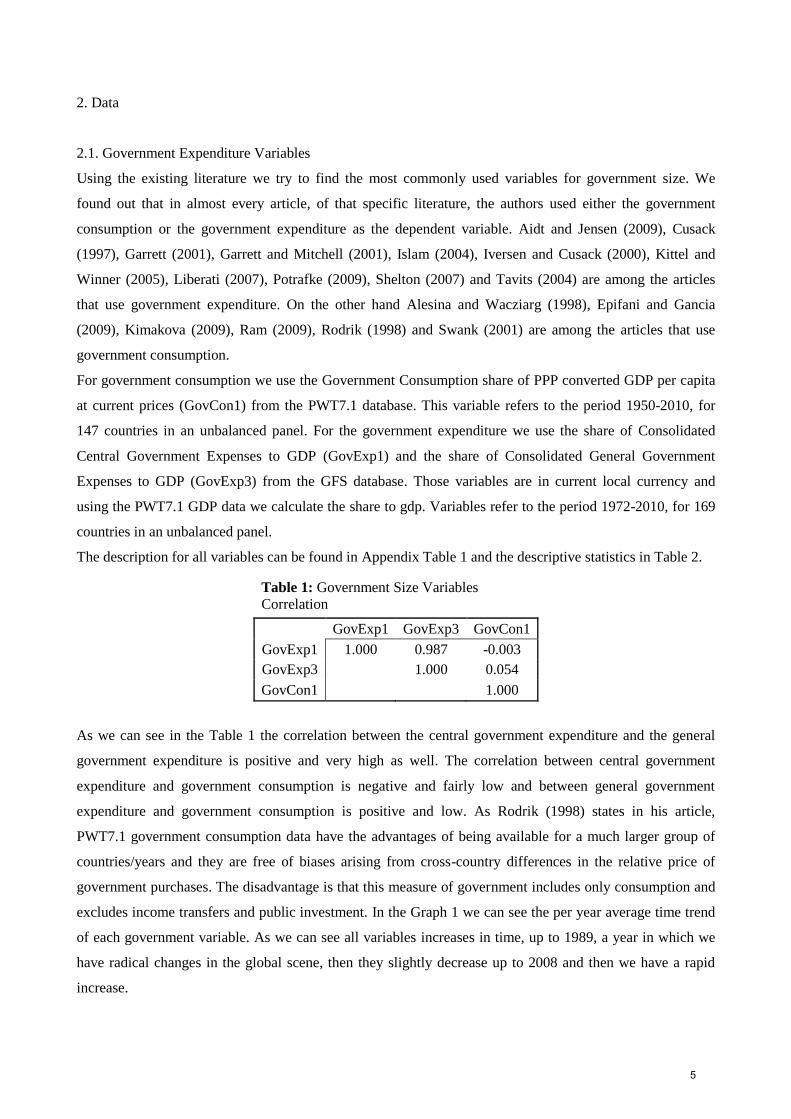
Table 1: Government Size Variables
Correlation
GovExp1 GovExp3 GovCon1
GovExp1 1.000 0.987 -0.003
GovExp3 1.000 0.054
GovCon1 1.000
As we can see in the Table 1 the correlation between the central government expenditure and the general
government expenditure is positive and very high as well. The correlation between central government
expenditure and government consumption is negative and fairly low and between general government
expenditure and government consumption is positive and low. As Rodrik (1998) states in his article,
PWT7.1 government consumption data have the advantages of being available for a much larger group of
countries/years and they are free of biases arising from cross-country differences in the relative price of
government purchases. The disadvantage is that this measure of government includes only consumption and
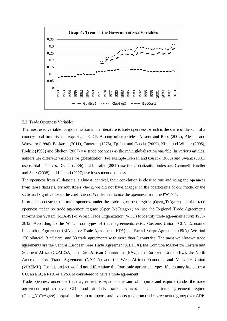
excludes income transfers and public investment. In the Graph 1 we can see the per year average time trend
of each government variable. As we can see all variables increases in time, up to 1989, a year in which we
have radical changes in the global scene, then they slightly decrease up to 2008 and then we have a rapid
increase.
5
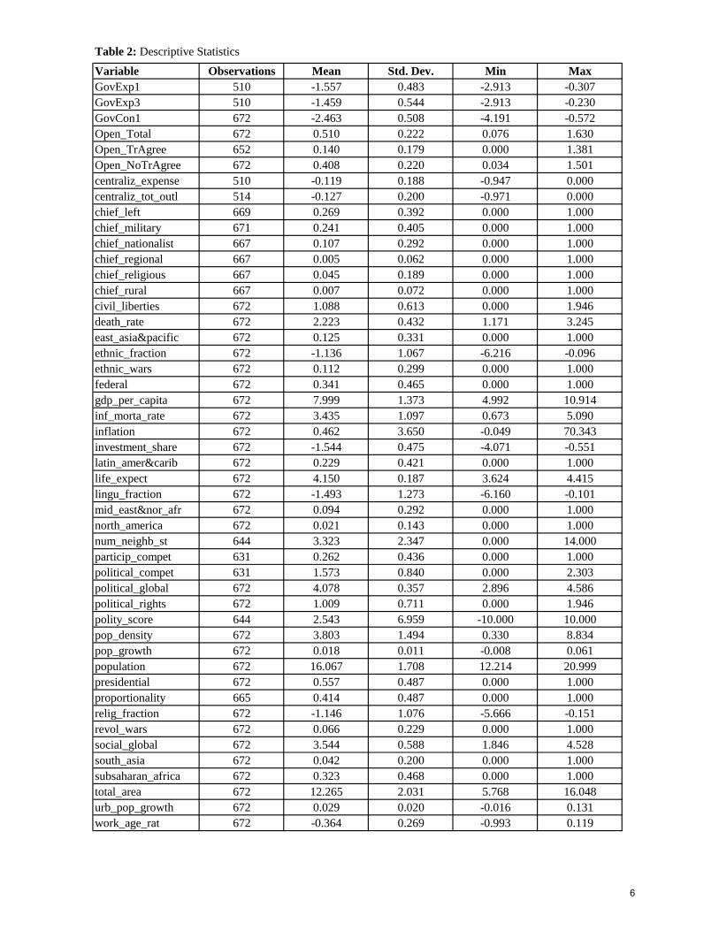
Variable Observations Mean Std. Dev. Min Max
GovExp1 510 -1.557 0.483 -2.913 -0.307
GovExp3 510 -1.459 0.544 -2.913 -0.230
GovCon1 672 -2.463 0.508 -4.191 -0.572
Open_Total 672 0.510 0.222 0.076 1.630
Open_TrAgree 652 0.140 0.179 0.000 1.381
Open_NoTrAgree 672 0.408 0.220 0.034 1.501
centraliz_expense 510 -0.119 0.188 -0.947 0.000
centraliz_tot_outl 514 -0.127 0.200 -0.971 0.000
chief_left 669 0.269 0.392 0.000 1.000
chief_military 671 0.241 0.405 0.000 1.000
chief_nationalist 667 0.107 0.292 0.000 1.000
chief_regional 667 0.005 0.062 0.000 1.000
chief_religious 667 0.045 0.189 0.000 1.000
chief_rural 667 0.007 0.072 0.000 1.000
civil_liberties 672 1.088 0.613 0.000 1.946
death_rate 672 2.223 0.432 1.171 3.245
east_asia&pacific 672 0.125 0.331 0.000 1.000
ethnic_fraction 672 -1.136 1.067 -6.216 -0.096
ethnic_wars 672 0.112 0.299 0.000 1.000
federal 672 0.341 0.465 0.000 1.000
gdp_per_capita 672 7.999 1.373 4.992 10.914
inf_morta_rate 672 3.435 1.097 0.673 5.090
inflation 672 0.462 3.650 -0.049 70.343
investment_share 672 -1.544 0.475 -4.071 -0.551
latin_amer&carib 672 0.229 0.421 0.000 1.000
life_expect 672 4.150 0.187 3.624 4.415
lingu_fraction 672 -1.493 1.273 -6.160 -0.101
mid_east&nor_afr 672 0.094 0.292 0.000 1.000
north_america 672 0.021 0.143 0.000 1.000
num_neighb_st 644 3.323 2.347 0.000 14.000
particip_compet 631 0.262 0.436 0.000 1.000
political_compet 631 1.573 0.840 0.000 2.303
political_global 672 4.078 0.357 2.896 4.586
political_rights 672 1.009 0.711 0.000 1.946
polity_score 644 2.543 6.959 -10.000 10.000
pop_density 672 3.803 1.494 0.330 8.834
pop_growth 672 0.018 0.011 -0.008 0.061
population 672 16.067 1.708 12.214 20.999
presidential 672 0.557 0.487 0.000 1.000
proportionality 665 0.414 0.487 0.000 1.000
relig_fraction 672 -1.146 1.076 -5.666 -0.151
revol_wars 672 0.066 0.229 0.000 1.000
social_global 672 3.544 0.588 1.846 4.528
south_asia 672 0.042 0.200 0.000 1.000
subsaharan_africa 672 0.323 0.468 0.000 1.000
total_area 672 12.265 2.031 5.768 16.048
urb_pop_growth 672 0.029 0.020 -0.016 0.131
work_age_rat 672 -0.364 0.269 -0.993 0.119
Table 2: Descriptive Statistics
6
2.2. Trade Openness Variables
The most used variable for globalization in the literature is trade openness, which is the share of the sum of a
country total imports and exports, in GDP. Among other articles, Adsera and Boix (2002), Alesina and
Wacziarg (1998), Baskaran (2011), Cameron (1978), Epifani and Gancia (2009), Kittel and Winner (2005),
Rodrik (1998) and Shelton (2007) use trade openness as the main globalization variable. In various articles,
authors use different variables for globalization. For example Iversen and Cusack (2000) and Swank (2001)
use capital openness, Dreher (2006) and Potrafke (2009) use the globalization index and Gemmell, Kneller
and Sanz (2008) and Liberati (2007) use investment openness.
The openness from all datasets is almost identical, their correlation is close to one and using the openness
from those datasets, for robustness check, we did not have changes in the coefficients of our model or the
statistical significance of the coefficients. We decided to use the openness from the PWT7.1.
In order to construct the trade openness under the trade agreement regime (Open_TrAgree) and the trade
openness under no trade agreement regime (Open_NoTrAgree) we use the Regional Trade Agreements
Information System (RTA-IS) of World Trade Organization (WTO) to identify trade agreements from 1958-
2012. According to the WTO, four types of trade agreements exist: Customs Union (CU), Economic
Integration Agreement (EIA), Free Trade Agreement (FTA) and Partial Scope Agreement (PSA). We find
136 bilateral, 3 trilateral and 33 trade agreements with more than 3 countries. The most well-known trade
agreements are the Central European Free Trade Agreement (CEFTA), the Common Market for Eastern and
Southern Africa (COMESA), the East African Community (EAC), the European Union (EU), the North
American Free Trade Agreement (NAFTA) and the West African Economic and Monetary Union
(WAEMU). For this project we did not differentiate the four trade agreement types. If a country has either a
CU, an EIA, a FTA or a PSA is considered to have a trade agreement.
Trade openness under the trade agreement is equal to the sum of imports and exports (under the trade
agreement regime) over GDP and similarly trade openness under no trade agreement regime
(Open_NoTrAgree) is equal to the sum of imports and exports (under no trade agreement regime) over GDP.
0
0.05
0.1
0.15
0.2
0.25
0.3
0.35
195
0
195
3
195
6
195
9
196
2
196
5
196
8
197
1
197
4
197
7
198
0
198
3
198
6
198
9
199
2
199
5
199
8
200
1
200
4
200
7
201
0
Graph1: Trend of the Government Size Variables
GovExp1 GovExp3 GovCon1
7
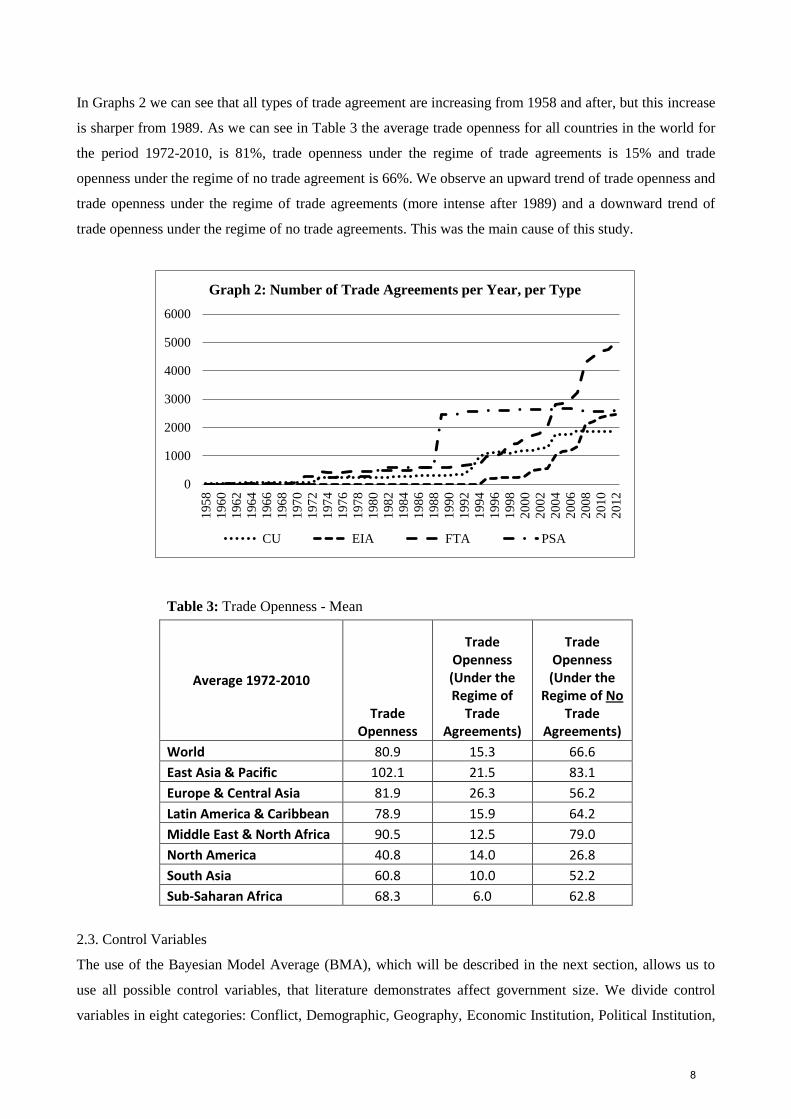
In Graphs 2 we can see that all types of trade agreement are increasing from 1958 and after, but this increase
is sharper from 1989. As we can see in Table 3 the average trade openness for all countries in the world for
the period 1972-2010, is 81%, trade openness under the regime of trade agreements is 15% and trade
openness under the regime of no trade agreement is 66%. We observe an upward trend of trade openness and
trade openness under the regime of trade agreements (more intense after 1989) and a downward trend of
trade openness under the regime of no trade agreements. This was the main cause of this study.
Table 3: Trade Openness - Mean
Average 1972-2010
Trade Openness
Trade Openness (Under the Regime of
Trade Agreements)
Trade Openness (Under the
Regime of No Trade
Agreements)
World 80.9 15.3 66.6
East Asia & Pacific 102.1 21.5 83.1
Europe & Central Asia 81.9 26.3 56.2
Latin America & Caribbean 78.9 15.9 64.2
Middle East & North Africa 90.5 12.5 79.0
North America 40.8 14.0 26.8
South Asia 60.8 10.0 52.2
Sub-Saharan Africa 68.3 6.0 62.8
2.3. Control Variables
The use of the Bayesian Model Average (BMA), which will be described in the next section, allows us to
use all possible control variables, that literature demonstrates affect government size. We divide control
variables in eight categories: Conflict, Demographic, Geography, Economic Institution, Political Institution,
0
1000
2000
3000
4000
5000
6000
195
8
196
0
196
2
196
4
196
6
196
8
197
0
197
2
197
4
197
6
197
8
198
0
198
2
198
4
198
6
198
8
199
0
199
2
199
4
199
6
199
8
200
0
200
2
200
4
200
6
200
8
201
0
201
2
Graph 2: Number of Trade Agreements per Year, per Type
CU EIA FTA PSA
8
Macro Policy, Politics and Trade variables. The databases we use are the Cross-National Time-Series Data
(CNTS) database, the Political Institutions (DPI) database, the Freedom House (FH) database, the
International Country Risk Guide (ICRG) database, the KOF Index of Globalization (KOF) database, the
NYU Development Research Institute (NYU) database, the Polity IV (PIV) database, the Penn World Table
7.1 (PWT7.1) database, the Quality of Government Institute (QoG) database and the World Development
Indicators (WDI) database. We run 71 specifications using more than 140 variables, in order to find out
which of those affect government expenditure and/or government consumption. After removing the
variables that were not significant in none of the 71 specifications we have 50 independent variables in the
final model. More information about the variables can be found in Appendix Tables 1-2.
2.3.1. Conflict Variables
In the final model we used the ethnic wars (ethnic_wars) and revolutionary wars (revol_wars) dummies from
the PIV database. We expect that war variables will positively affect government size. Eterovic and Eterovic
(2012) find a positive coefficient for the armed conflict dummy and Ferris, Park and Winer (2008) find that
the period between the two World Wars and the period after WWII (peaceful periods) negatively affect the
government size. We also tested the number of armed activity, sabotage, or bombings carried on by
independent bands of citizens or irregular forces, the number of illegal or forced change in the top
government elite, the number peaceful public gathering of at least 100 people, the number of strike of 1,000
or more industrial or service workers, the number of violent demonstration or clash of more than 100
citizens involving the use of physical force, the weighted conflict index and the genocide and politicide
dummy. We found that none of those variables affect any of our dependent variables in any specification.
2.3.2. Demographic Variables
In the final model we used population (population) from PWT7.1 database, the percentage of working-age
population (work_age_rat), the death rate (death_rate), the infant mortality rate (inf_morta_rate), the life
expectancy (life_expect), the population density (pop_density), the population growth (pop_growth) and the
urban population growth (urb_pop_growth) from WDI database. We expect that death rate and infant
mortality rate will positively affect government size and the rest variables will negatively affect it. In
literature the effect of population is ambiguous. Articles such as Epifani and Gancia (2009), Kittel and
Winner (2005) and Grossman (1989, 1992) show that population has a positive effect while articles such as
Alesina and Wacziarg (1998), Benarroch and Pandey (2008), Liberati (2007) and Prohl and Schneider
(2009) show it has a negative effect. The same is true for urbanization. Alesina and Wacziarg (1998),
Benarroch and Pandey (2008), Pickup (2006) and Rodrik (1998) conclude that urbanization negatively
affects the government size while Aidt and Jensen (2009), Jin and Zou (2002), Khattry and Rao (2002) and
Kimakova (2009) conclude that urbanization affects it positively. In the case of dependency ratio the vast
majority of articles, like Benarroch and Pandey (2008), Garrett and Mitchell (2001), Kittel and Winner
(2005), Rodrik (1998) and Shelton (2007) find out that dependency ratio positively affects the government
expenditure (in our case we have the working population, which is one minus the dependency ratio, so we
expect a negative result). Baskaran (2011), Cassette and Paty (2010) and Lott and Kenny (1999), which
9
tested population density find a negative effect. We also tested the birth rate and the rural population growth
and came to the conclusion that none of those variables affect any of our dependent variables in any
specification.
2.3.3. Geographic Variables
In the final model we used the number of neighboring states sharing a border with the identified state
(num_neighb_st), the ethnic (ethnic_fraction), the linguistic (lingu_fraction) and the religious
fractionalization (relig_fraction) index from QoG database and the country total area (total_area) from WDI
database. We expect a positive coefficient for all variables. Adsera and Boix (2002), Bretschger and Hettich
(2002) and Garrett (2001) found that the country area positively affects government size. Alesina
Devleeschauwer, Easterly, Kurlat and Wacziarg (2003) found that ethnic and linguistic fractionalization has
a negative effect on it. We also tested three geographical dummies: if a country is an island, landlocked or
has a tropical climate, and found out that none of those variables affect any of our dependent variables in
any specification.
2.3.4. Economic Institution Variables
In the final model we used the civil liberties index (civil_liberties) from FH database. We expect a negative
coefficient, since the variable is smaller for countries with more respect to civil liberties. Adsera and Boix
(2002) found a negative coefficient for the democratic index (civil liberties index can be considered as a
proxy for democracy) while Zakaria and Shakoor (2011) found a positive coefficient. We also tested various
risk variables from ICRG database, such as budget balance, current account as % of xgs, current account as
% of gdp, debt service, exchange rate stability, foreign debt, gdp growth, per capita gdp, inflation and
international liquidity risk, as well as the investment profile and socioeconomic conditions of the country.
None of those variables affect any of our dependent variables in any specification.
2.3.5. Political Institution Variables
In the final model we used five dummy variables about the chief executive party from DPI database: left
(chief_left), nationalist (chief_nationalist), regional (chief_regional), religious (chief_religious) and rural
(chief_rural). Also we use a dummy, if the chief executive is a military officer (chief_military) from DPI,
the political rights index (political_rights) from FH database and the revised combined polity score
(polity_score) from PIV database. We expect that if the chief executive party is left-wing or nationalist this
will positively affect the government size. We expect a negative coefficient for political rights index, since
the variable is smaller for countries with more respect to political rights, and a positive coefficient for the
revised combined polity score. As we mention earlier Adsera and Boix (2002) found a negative coefficient
for the democratic index, while Zakaria and Shakoor (2011) found a positive coefficient. Cameron (1978),
Iversen and Cusack (2000) and Kittel and Winner (2005) found that left-wing, social democratic or labor
parties positively affect the governments expenditure. We also tested two extra dummies from the DPI
database: if the chief executive party controls all relevant houses and if there is a finite term in office for the
chief executive. Moreover we tested ten indices from ICRG database: bureaucracy quality, corruption,
democratic accountability, ethnic tensions, external conflict, government stability, internal conflict, law &
10

order, military in politics and religious tensions. From the PIV database we tested four dummies: if an
executive have unlimited authority, if the executive is recruit by election, if the executive recruitment is
open to everybody if the chief executive recruitment is regulated. Finally we tested five dummies from the
QoG database: if the judiciary is independent and if the legal origin of the country is British, French,
German or Scandinavian. None of those variables affect any of our dependent variables in any specification.
2.3.6. Macro Policy Variables
In the final model we used two centralization variables (centraliz_expense and centraliz_tot_outl) from the
GFS database, as well as the investment share to gdp (investment_share) and the gdp per capita
(gdp_per_capita) from the PWT7.1 database and the inflation (inflation) from the WDI database. According
to Wagner’s law we expect that gdp per capita have a positive effect on government size. The Leviathan
Hypothesis from Brennan and Buchanan (1980) states that government intrusion into the economy will be
smaller when the public sector is decentralized. Under this hypothesis we expect a positive coefficient of
centralization (in our case centralization is the share of central to general government expenditure) on central
government expenditure and a negative coefficient on general government expenditure. Alesina and
Wacziarg (1998), Epifani and Gancia (2009) and Rodrik (1998) find a negative sign for gdp per capita,
while Adsera and Boix (2002), Garrett (2001) and Islam (2004) find a positive coefficient. As for
decentralization, Grossman (1989) and Marlow (1988) find a negative effect while Baskaran (2011) and
Cassette and Paty (2010) find a positive effect. We also tested for the effect of gdp growth, current account
balance, foreign direct investment, gross capital formation, gross savings and total reserves. None of those
variables affect any of our dependent variables in any specification.
2.3.7. Politic Variables
In the final model we used four political dummies: the electoral rule (proportionality) and type of regime
(presidential) from the DPI database, if participation is competitive (particip_compet) from the PIV database
and the system of government (federal) from the QoG database. Also we used the political competition
index (political_compet) from the PIV database. Aidt and Jensen (2009) and Eterovic and Eterovic (2012)
find a negative coefficient for political competition, Eterovic and Eterovic (2012), Iversen and Cusack
(2000) and Mueller and Stratmann (2003) find a positive coefficient for participation index, Aidt and Jensen
(2009) and Baraldi (2008) find a negative coefficient for the proportional electoral rule and Prohl and
Schneider (2009) find a negative coefficient for the majoritarian electoral system, while Tavits (2004) find a
positive coefficient. We also tested the polarization index, the vote share of government and opposition
parties and the executive and/or legislative election year dummy. None of those variables affect any of our
dependent variables in any specification.
2.3.8. Trade Variables
In the final model, except from the trade openness variables which was previously explained, we used the
political (political_global) and social globalization index (social_global) from KOF database. We also tested
the terms of trade adjustment and four dummies about the export profile of the country: fuels, manufactures,
11
nonfuel primary products and services. None of those variables affect any of our dependent variables in any
specification.
2.3.9. Other Variables
Except from the control variables mentioned above in the final model we use time dummies and regional
dummies from the WDI database: East Asia & Pacific, Latin America & Caribbean, Middle East & North
Africa, North America, South Asia and Sub-Saharan Africa region. Also we run various specifications using
interaction terms. We use the squares of area size, civil liberties, per capita income, political rights,
population and revised combined polity score as well as the interaction of those variables with all the trade
openness variables.
2.4. Final Dataset
Time: Because of the use of different databases, which cover different time periods, we had to find the
common period range to use. We ended up using data from 1976-2010. In order to avoid business cycle we
used a 5-year average technique in all variables. We ended up with seven time periods: 1976-1980, 1981-
1985, 1986-1990, 1991-1995, 1996-2000, 2001-2005 and 2006-2010.
Countries: We decided to use a balanced panel of countries. As a result, for each of the seven depended
variables, we used countries with full observation for all variables, for all time periods. We did this in order
to avoid the effect on the results from “newly-born” countries, such as Russia or other former USSR
countries. For each of the government variable we can see the countries we used in Appendix Table 3.
Variables: Finally we had to choose the way that a variable would enter the model. By this we mean if the
variable will enter as a five-year average, the natural logarithm of the five-year average, the initial value for
each time period window or the natural logarithm of the initial value. So as to decide the way we consulted
the literature and ran different specifications, to see if our results are robust. All dependent variables are the
logarithm of the five-year average. The openness variables are entering the final model as the logarithm of
the five-year average, but we used the expression ln(1+X) instead of ln(X) in order not to reduce our sample
(for a lot of countries, especially for the first years, the trade openness under the regime of no trade
agreement was zero). For gdp per capita we used the logarithm of the initial value for each time period (this
is the common use in the literature). Finally all other control variables are entering as the logarithm of the
five-year average. In the case that we were not able to calculate the logarithm of the five-year average (in
case of zero or negative values and in case of dummies that did not vary through time), we used the five-year
average. For each of the government variables we can see the variables and the way they enter in the model
in Appendix Table 4. Finally in Table 2 we have the descriptive statistics for all variables.
12
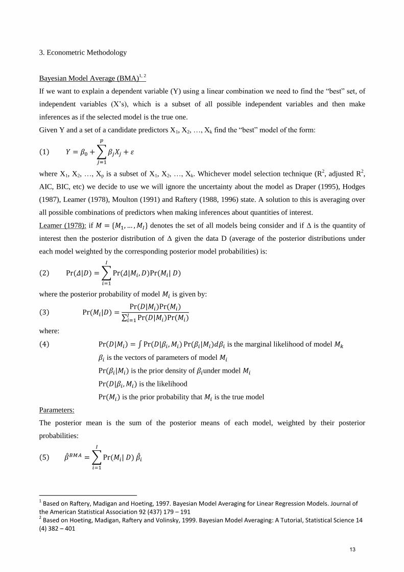
3. Econometric Methodology
Bayesian Model Average (BMA)1, 2
If we want to explain a dependent variable (Y) using a linear combination we need to find the “best” set, of
independent variables (X’s), which is a subset of all possible independent variables and then make
inferences as if the selected model is the true one.
Given Y and a set of a candidate predictors X1, X2, …, Xk find the “best” model of the form:
( ) ∑
where X1, X2, …, Xp is a subset of X1, X2, …, Xk. Whichever model selection technique (R2, adjusted R
2,
AIC, BIC, etc) we decide to use we will ignore the uncertainty about the model as Draper (1995), Hodges
(1987), Leamer (1978), Moulton (1991) and Raftery (1988, 1996) state. A solution to this is averaging over
all possible combinations of predictors when making inferences about quantities of interest.
Leamer (1978): if * + denotes the set of all models being consider and if Δ is the quantity of
interest then the posterior distribution of Δ given the data D (average of the posterior distributions under
each model weighted by the corresponding posterior model probabilities) is:
( ) ( ) ∑ ( ) ( )
where the posterior probability of model is given by:
( ) ( ) ( ) ( )
∑ ( ) ( )
where:
( ) ( ) ∫ ( ) ( ) is the marginal likelihood of model
is the vectors of parameters of model
( ) is the prior density of under model
( ) is the likelihood
( ) is the prior probability that is the true model
Parameters:
The posterior mean is the sum of the posterior means of each model, weighted by their posterior
probabilities:
( ) ̂ ∑ ( ) ̂
1 Based on Raftery, Madigan and Hoeting, 1997. Bayesian Model Averaging for Linear Regression Models. Journal of
the American Statistical Association 92 (437) 179 – 191 2 Based on Hoeting, Madigan, Raftery and Volinsky, 1999. Bayesian Model Averaging: A Tutorial, Statistical Science 14
(4) 382 – 401
13
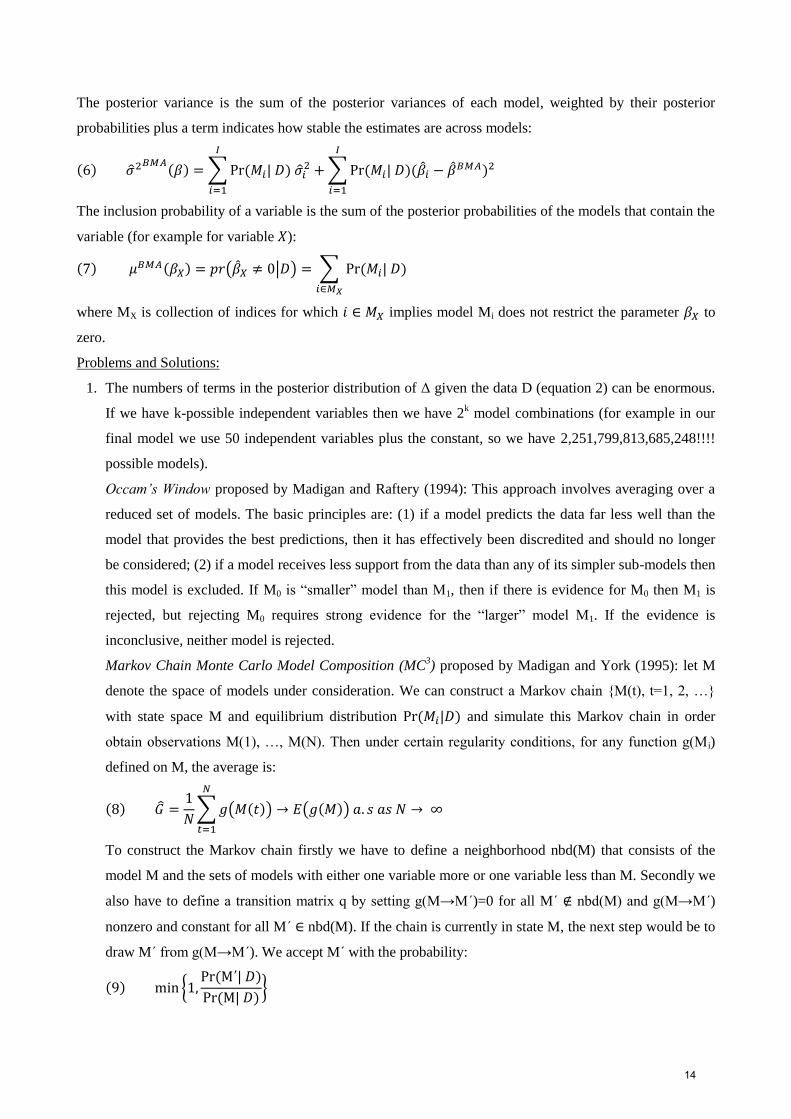
The posterior variance is the sum of the posterior variances of each model, weighted by their posterior
probabilities plus a term indicates how stable the estimates are across models:
( ) ̂
( ) ∑ ( ) ̂
∑ ( )( ̂ ̂ )
The inclusion probability of a variable is the sum of the posterior probabilities of the models that contain the
variable (for example for variable ):
( ) ( ) ( ̂ | ) ∑ ( )
where MX is collection of indices for which implies model Mi does not restrict the parameter to
zero.
Problems and Solutions:
1. The numbers of terms in the posterior distribution of Δ given the data D (equation 2) can be enormous.
If we have k-possible independent variables then we have 2k model combinations (for example in our
final model we use 50 independent variables plus the constant, so we have 2,251,799,813,685,248!!!!
possible models).
Occam’s Window proposed by Madigan and Raftery (1994): This approach involves averaging over a
reduced set of models. The basic principles are: (1) if a model predicts the data far less well than the
model that provides the best predictions, then it has effectively been discredited and should no longer
be considered; (2) if a model receives less support from the data than any of its simpler sub-models then
this model is excluded. If M0 is “smaller” model than M1, then if there is evidence for M0 then M1 is
rejected, but rejecting M0 requires strong evidence for the “larger” model M1. If the evidence is
inconclusive, neither model is rejected.
Markov Chain Monte Carlo Model Composition (MC3) proposed by Madigan and York (1995): let M
denote the space of models under consideration. We can construct a Markov chain {M(t), t=1, 2, …}
with state space M and equilibrium distribution ( ) and simulate this Markov chain in order
obtain observations M(1), …, M(N). Then under certain regularity conditions, for any function g(Mi)
defined on M, the average is:
( ) ̂
∑ ( ( ))
( ( ))
To construct the Markov chain firstly we have to define a neighborhood nbd(M) that consists of the
model M and the sets of models with either one variable more or one variable less than M. Secondly we
also have to define a transition matrix q by setting g(M→M΄)=0 for all M΄ ∉ nbd(M) and g(M→M΄)
nonzero and constant for all M΄ nbd(M). If the chain is currently in state M, the next step would be to
draw M΄ from g(M→M΄). We accept M΄ with the probability:
( ) { ( )
( )}
14
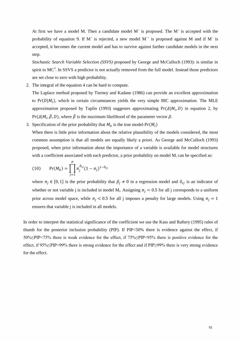
At first we have a model M. Then a candidate model M΄ is proposed. The M΄ is accepted with the
probability of equation 9. If M΄ is rejected, a new model M΄΄ is proposed against M and if M΄ is
accepted, it becomes the current model and has to survive against further candidate models in the next
step.
Stochastic Search Variable Selection (SSVS) proposed by George and McCulloch (1993): is similar in
spirit to MC3. In SSVS a predictor is not actually removed from the full model. Instead those predictors
are set close to zero with high probability.
2. The integral of the equation 4 can be hard to compute.
The Laplace method proposed by Tierney and Kadane (1986) can provide an excellent approximation
to ( ), which in certain circumstances yields the very simple BIC approximation. The MLE
approximation proposed by Taplin (1993) suggestes approximating ( ) in equation 2, by
( ̂ ), where ̂ is the maximum likelihood of the parameter vector .
3. Specification of the prior probability that is the true model- ( )
When there is little prior information about the relative plausibility of the models considered, the most
common assumption is that all models are equally likely a priori. As George and McCulloch (1993)
proposed, when prior information about the importance of a variable is available for model structures
with a coefficient associated with each predictor, a prior probability on model Mi can be specified as:
( ) ( ) ∏
( )
where , - is the prior probability that in a regression model and is an indicator of
whether or not variable j is included in model Mi. Assigning for all j corresponds to a uniform
prior across model space, while for all j imposes a penalty for large models. Using
ensures that variable j is included in all models.
In order to interpret the statistical significance of the coefficient we use the Kass and Raftery (1995) rules of
thumb for the posterior inclusion probability (PIP). If PIP<50% there is evidence against the effect, if
50%≤PIP<75% there is weak evidence for the effect, if 75%≤PIP<95% there is positive evidence for the
effect, if 95%≤PIP<99% there is strong evidence for the effect and if PIP≥99% there is very strong evidence
for the effect.
15
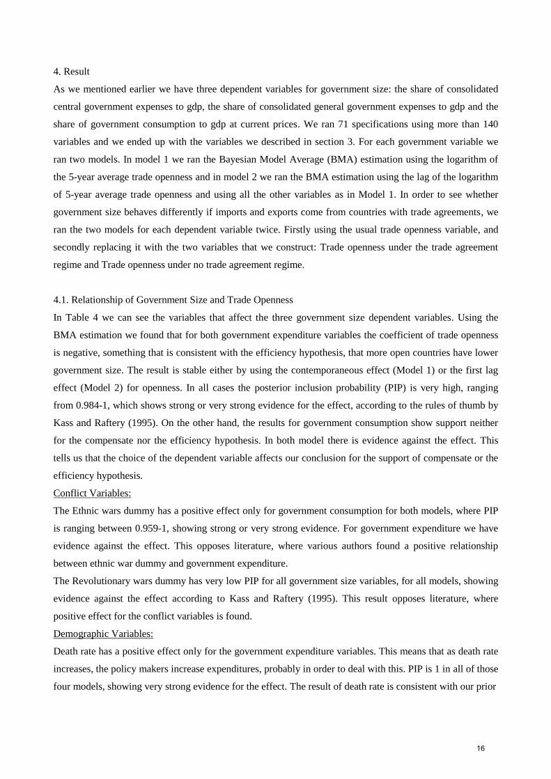
4. Result
As we mentioned earlier we have three dependent variables for government size: the share of consolidated
central government expenses to gdp, the share of consolidated general government expenses to gdp and the
share of government consumption to gdp at current prices. We ran 71 specifications using more than 140
variables and we ended up with the variables we described in section 3. For each government variable we
ran two models. In model 1 we ran the Bayesian Model Average (BMA) estimation using the logarithm of
the 5-year average trade openness and in model 2 we ran the BMA estimation using the lag of the logarithm
of 5-year average trade openness and using all the other variables as in Model 1. In order to see whether
government size behaves differently if imports and exports come from countries with trade agreements, we
ran the two models for each dependent variable twice. Firstly using the usual trade openness variable, and
secondly replacing it with the two variables that we construct: Trade openness under the trade agreement
regime and Trade openness under no trade agreement regime.
4.1. Relationship of Government Size and Trade Openness
In Table 4 we can see the variables that affect the three government size dependent variables. Using the
BMA estimation we found that for both government expenditure variables the coefficient of trade openness
is negative, something that is consistent with the efficiency hypothesis, that more open countries have lower
government size. The result is stable either by using the contemporaneous effect (Model 1) or the first lag
effect (Model 2) for openness. In all cases the posterior inclusion probability (PIP) is very high, ranging
from 0.984-1, which shows strong or very strong evidence for the effect, according to the rules of thumb by
Kass and Raftery (1995). On the other hand, the results for government consumption show support neither
for the compensate nor the efficiency hypothesis. In both model there is evidence against the effect. This
tells us that the choice of the dependent variable affects our conclusion for the support of compensate or the
efficiency hypothesis.
Conflict Variables:
The Ethnic wars dummy has a positive effect only for government consumption for both models, where PIP
is ranging between 0.959-1, showing strong or very strong evidence. For government expenditure we have
evidence against the effect. This opposes literature, where various authors found a positive relationship
between ethnic war dummy and government expenditure.
The Revolutionary wars dummy has very low PIP for all government size variables, for all models, showing
evidence against the effect according to Kass and Raftery (1995). This result opposes literature, where
positive effect for the conflict variables is found.
Demographic Variables:
Death rate has a positive effect only for the government expenditure variables. This means that as death rate
increases, the policy makers increase expenditures, probably in order to deal with this. PIP is 1 in all of those
four models, showing very strong evidence for the effect. The result of death rate is consistent with our prior
16

Conflict Variables
ethnic_wars 0.0014 0.0011 0.0014 0.0011 0.2588 *** 0.2456 **
(0.054) (0.049) (0.022) (0.039) (1.000) (0.959)
revol_wars -0.0002 -0.0005 0.0006 0.0013 -0.0864 -0.0405
(0.018) (0.048) (0.077) (0.049) (0.454) (0.220)
Demographic Variables
death_rate 0.4928 *** 0.5064 *** 0.4671 *** 0.4808 *** -0.0043 -0.0015
(1.000) (1.000) (1.000) (1.000) (0.068) (0.082)
inf_morta_rate -0.2892 *** -0.2778 *** -0.3101 *** -0.2943 *** 0.0009 0.0007
(1.000) (1.000) (1.000) (1.000) (0.071) (0.023)
life_expect 0.0099 -0.0018 0.0149 -0.0042 0.0024 0.0295
(0.143) (0.094) (0.132) (0.094) (0.011) (0.065)
pop_density 0.0002 -0.0001 -0.0002 -0.0003 3.0111 *** 2.9915 ***
(0.037) (0.027) (0.024) (0.027) (1.000) (1.000)
pop_growth -0.2096 -0.0901 -0.2965 -0.1245 0.0181 -0.0289
(0.065) (0.069) (0.132) (0.037) (0.020) (0.071)
population -0.0007 -0.0004 -0.0006 -0.0001 -3.1143 *** -3.0939 ***
(0.046) (0.046) (0.050) (0.048) (1.000) (1.000)
urb_pop_growth -0.5044 -0.4431 -0.6789 -0.4278 -0.0601 -0.0709
(0.241) (0.245) (0.292) (0.175) (0.053) (0.079)
work_age_rat -0.0008 0.0003 0.0071 0.0014 0.0050 0.0197
(0.081) (0.017) (0.090) (0.033) (0.032) (0.135)
Geographic Variables
ethnic_fraction -0.0014 -0.0010 -0.0021 -0.0002 0.0197 0.0147
(0.100) (0.096) (0.160) (0.040) (0.390) (0.316)
lingu_fraction -0.0028 -0.0032 -0.0031 -0.0051 -0.0017 -0.0007
(0.163) (0.187) (0.177) (0.219) (0.058) (0.052)
relig_fraction 0.0352 0.0336 0.0271 0.0291 0.0918 *** 0.0885 ***
(0.743) (0.698) (0.596) (0.618) (1.000) (1.000)
num_neighb_st 0.0465 *** 0.0449 *** 0.0427 *** 0.0425 ***
(1.000) (1.000) (1.000) (1.000)
total_area -0.0004 -0.0013 -0.0002 0.0006 3.0492 *** 3.0278 ***
(0.037) (0.156) (0.024) (0.065) (1.000) (1.000)
Economic Institution Variables
civil_liberties -0.0740 -0.0557 -0.0721 -0.0839 0.0006 0.0014
(0.568) (0.466) (0.512) (0.551) (0.034) (0.051)
Table 4: Results - Relationship of Government Size and Trade Openness
Model 1 Model 2
Dependent Variable Central Government
Expenditure
Model 2
Government Consumption
Model 1 Model 2
General Government
Expenditure
Model 1
17
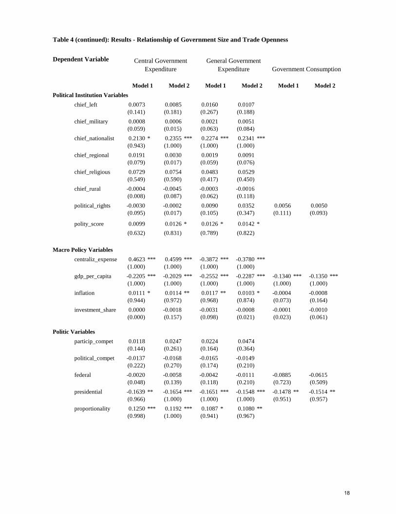
Political Institution Variables
chief_left 0.0073 0.0085 0.0160 0.0107
(0.141) (0.181) (0.267) (0.188)
chief_military 0.0008 0.0006 0.0021 0.0051
(0.059) (0.015) (0.063) (0.084)
chief_nationalist 0.2130 * 0.2355 *** 0.2274 *** 0.2341 ***
(0.943) (1.000) (1.000) (1.000)
chief_regional 0.0191 0.0030 0.0019 0.0091
(0.079) (0.017) (0.059) (0.076)
chief_religious 0.0729 0.0754 0.0483 0.0529
(0.549) (0.590) (0.417) (0.450)
chief_rural -0.0004 -0.0045 -0.0003 -0.0016
(0.008) (0.087) (0.062) (0.118)
political_rights -0.0030 -0.0002 0.0090 0.0352 0.0056 0.0050
(0.095) (0.017) (0.105) (0.347) (0.111) (0.093)
polity_score 0.0099 0.0126 * 0.0126 * 0.0142 *
(0.632) (0.831) (0.789) (0.822)
Macro Policy Variables
centraliz_expense 0.4623 *** 0.4599 *** -0.3872 *** -0.3780 ***
(1.000) (1.000) (1.000) (1.000)
gdp_per_capita -0.2205 *** -0.2029 *** -0.2552 *** -0.2287 *** -0.1340 *** -0.1350 ***
(1.000) (1.000) (1.000) (1.000) (1.000) (1.000)
inflation 0.0111 * 0.0114 ** 0.0117 ** 0.0103 * -0.0004 -0.0008
(0.944) (0.972) (0.968) (0.874) (0.073) (0.164)
investment_share 0.0000 -0.0018 -0.0031 -0.0008 -0.0001 -0.0010
(0.000) (0.157) (0.098) (0.021) (0.023) (0.061)
Politic Variables
particip_compet 0.0118 0.0247 0.0224 0.0474
(0.144) (0.261) (0.164) (0.364)
political_compet -0.0137 -0.0168 -0.0165 -0.0149
(0.222) (0.270) (0.174) (0.210)
federal -0.0020 -0.0058 -0.0042 -0.0111 -0.0885 -0.0615
(0.048) (0.139) (0.118) (0.210) (0.723) (0.509)
presidential -0.1639 ** -0.1654 *** -0.1651 *** -0.1548 *** -0.1478 ** -0.1514 **
(0.966) (1.000) (1.000) (1.000) (0.951) (0.957)
proportionality 0.1250 *** 0.1192 *** 0.1087 * 0.1080 **
(0.998) (1.000) (0.941) (0.967)
Table 4 (continued): Results - Relationship of Government Size and Trade Openness
Dependent Variable Central Government
Expenditure
General Government
Expenditure Government Consumption
Model 2Model 1 Model 2 Model 1 Model 2 Model 1
18
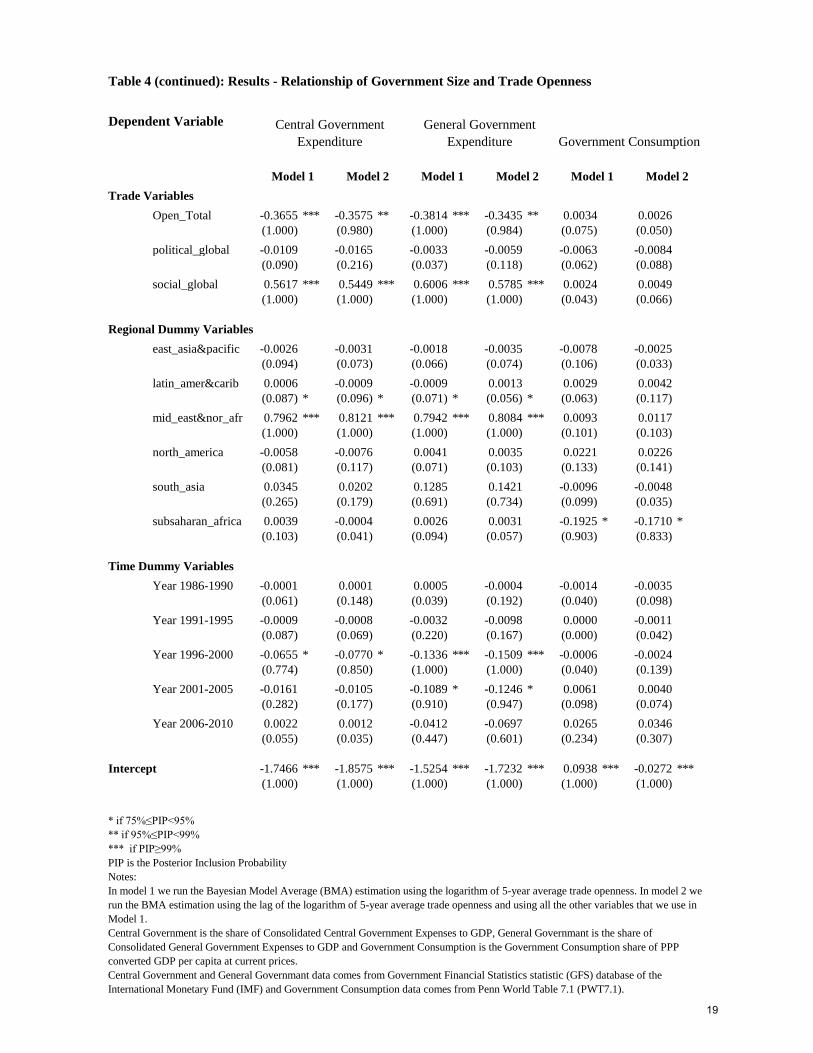
Trade Variables
Open_Total -0.3655 *** -0.3575 ** -0.3814 *** -0.3435 ** 0.0034 0.0026
(1.000) (0.980) (1.000) (0.984) (0.075) (0.050)
political_global -0.0109 -0.0165 -0.0033 -0.0059 -0.0063 -0.0084
(0.090) (0.216) (0.037) (0.118) (0.062) (0.088)
social_global 0.5617 *** 0.5449 *** 0.6006 *** 0.5785 *** 0.0024 0.0049
(1.000) (1.000) (1.000) (1.000) (0.043) (0.066)
Regional Dummy Variables
east_asia&pacific -0.0026 -0.0031 -0.0018 -0.0035 -0.0078 -0.0025
(0.094) (0.073) (0.066) (0.074) (0.106) (0.033)
latin_amer&carib 0.0006 -0.0009 -0.0009 0.0013 0.0029 0.0042
(0.087) * (0.096) * (0.071) * (0.056) * (0.063) (0.117)
mid_east&nor_afr 0.7962 *** 0.8121 *** 0.7942 *** 0.8084 *** 0.0093 0.0117
(1.000) (1.000) (1.000) (1.000) (0.101) (0.103)
north_america -0.0058 -0.0076 0.0041 0.0035 0.0221 0.0226
(0.081) (0.117) (0.071) (0.103) (0.133) (0.141)
south_asia 0.0345 0.0202 0.1285 0.1421 -0.0096 -0.0048
(0.265) (0.179) (0.691) (0.734) (0.099) (0.035)
subsaharan_africa 0.0039 -0.0004 0.0026 0.0031 -0.1925 * -0.1710 *
(0.103) (0.041) (0.094) (0.057) (0.903) (0.833)
Time Dummy Variables
Year 1986-1990 -0.0001 0.0001 0.0005 -0.0004 -0.0014 -0.0035
(0.061) (0.148) (0.039) (0.192) (0.040) (0.098)
Year 1991-1995 -0.0009 -0.0008 -0.0032 -0.0098 0.0000 -0.0011
(0.087) (0.069) (0.220) (0.167) (0.000) (0.042)
Year 1996-2000 -0.0655 * -0.0770 * -0.1336 *** -0.1509 *** -0.0006 -0.0024
(0.774) (0.850) (1.000) (1.000) (0.040) (0.139)
Year 2001-2005 -0.0161 -0.0105 -0.1089 * -0.1246 * 0.0061 0.0040
(0.282) (0.177) (0.910) (0.947) (0.098) (0.074)
Year 2006-2010 0.0022 0.0012 -0.0412 -0.0697 0.0265 0.0346
(0.055) (0.035) (0.447) (0.601) (0.234) (0.307)
Intercept -1.7466 *** -1.8575 *** -1.5254 *** -1.7232 *** 0.0938 *** -0.0272 ***
(1.000) (1.000) (1.000) (1.000) (1.000) (1.000)
Table 4 (continued): Results - Relationship of Government Size and Trade Openness
Dependent Variable Central Government
Expenditure
General Government
Expenditure Government Consumption
Model 2
* if 75%≤PIP<95%
** if 95%≤PIP<99%
*** if PIP≥99%
PIP is the Posterior Inclusion Probability
Notes:
In model 1 we run the Bayesian Model Average (BMA) estimation using the logarithm of 5-year average trade openness. In model 2 we
run the BMA estimation using the lag of the logarithm of 5-year average trade openness and using all the other variables that we use in
Model 1.
Central Government is the share of Consolidated Central Government Expenses to GDP, General Governmant is the share of
Consolidated General Government Expenses to GDP and Government Consumption is the Government Consumption share of PPP
converted GDP per capita at current prices.
Central Government and General Governmant data comes from Government Financial Statistics statistic (GFS) database of the
International Monetary Fund (IMF) and Government Consumption data comes from Penn World Table 7.1 (PWT7.1).
Model 1 Model 2 Model 1 Model 2 Model 1
19

expectations. This is not true for the government consumption variable, where death rate has a very low PIP,
for all models, showing evidence against the effect according to Kass and Raftery (1995).
Infant mortality rate has a negative effect for the government expenditure variables. This shows that as
infant mortality rate increases, the policy makers decrease expenditures. PIP is 1 in all models,
demonstrating very strong evidence for the effect. If we use the government consumption as the dependent
variable, the results are different. Infant mortality rate has a very low PIP, for all models, showing evidence
against the effect according to Kass and Raftery (1995).
Life expectancy has very low PIP for all government size variables, for all models, showing evidence
against the effect according to Kass and Raftery (1995).
Population density has a very strong positive effect only for government consumption, with PIP equal to 1.
For both government expenditure variables population density shows evidence against the effect. Those
results opposes the literature, where they found a negative coefficient for government size, showing that as
the population per square km of land area increases, the policy makers decrease expenditures.
Population growth has very low PIP for all government size variables, for all models, showing evidence
against the effect according to Kass and Raftery (1995). This result opposes our prior expectations, where
we expected a negative effect.
Population has a strong negative effect for government consumption to gdp with PIP equal to 1 in both
models, showing a very strong evidence for the effect. This is not true for the government expenditure
variables, where we find evidence against the effect. The negative effect is consistent with a part of the
literature (since the effect is ambiguous) and shows that as population increases, the policy makers decrease
expenditures.
Urban population growth has very low PIP for all government size variables, for all models, showing
evidence against the effect according to Kass and Raftery (1995). This opposes literature where various
authors found either a negative or a positive effect.
Working age ratio has very low PIP for all government size variables, for all models, showing evidence
against the effect according to Kass and Raftery (1995). This opposes literature. The vast majority of the
literature found a negative effect and shows that as working age ratio increases, the policy makers decrease
expenditures, since the inhabitants that need social transfers decreased.
Geographic Variables:
The Ethnic, Linguistic and Religious fractionalization index has very low PIP for all government size
variables, for all models, showing evidence against the effect according to Kass and Raftery (1995). The
only exception is the very strong positive effect of religious fractionalization for both models if we use the
government consumption as the dependent variable. This shows that as the probability that two randomly
selected people from a given country will not belong to the same religious group increases, the policy
makers increase expenditures. In the literature ethnic and linguistic fractionalization indices have a negative
effect, which opposes our results.
20
The number of neighboring states sharing a border with the identified state has a very strong positive effect
on both government expenditure variables. This shows that countries with many neighbors tend to have
more government expenditures, probably in order to deal with this, in terms of external threads or migration.
The result of the number of neighboring states sharing a border with the identified state is consistent with
our prior expectations.
The country’s total area in square kilometers has a very strong positive effect only for government
consumption. This is consistent with literature findings and shows that bigger countries tend to have bigger
government consumption.
Economic Institution Variables:
The Civil liberties index has very low PIP for all government size variables, for all models, showing
evidence against the effect according to Kass and Raftery (1995). For Model 1, in the case of the central
government expenditure variable, and for the general government expenditure variable, PIP is ranging from
0.512-0.568, which shows weak evidence for the effect, according rules of thumb of Kass and Raftery
(1995). Those results opposes the literature, where various authors found that countries with greater respect
(smaller number of the index show greater respect) for civil liberties tend to have higher government
expenditures.
Political Institution Variables:
The orientation of the chief executive party (in our case if we test for a left-wing party), has a very low PIP
for all government size variables, for all models, showing evidence against the effect according to Kass and
Raftery (1995). This result opposes the literature, where a positive effect is found.
Whether the president is a military officer, then this will not affect either the government expenditure or the
government consumption. In all cases we have a very low PIP, showing evidence against the effect
according to Kass and Raftery (1995).
The background of the chief executive party (we test if the chief executive originates from a nationalist, a
regional, a religious or a rural parties) do not seem to affect government expenditure. The only exception is
when the chief executive party is nationalist. This affects the government expenditures positively. PIP is
very high, ranging from 0.943-1, which shows strong or very strong evidence for the effect, according rules
of thumb of Kass and Raftery (1995). In the case when we use the central government expenditure, when the
chief executive party is religious we have a weak positive evidence for the effect. In all other cases PIP
shows evidence against the effect
The Political rights index has very low PIP for all government size variables, for all models, showing
evidence against the effect according to Kass and Raftery (1995). This opposes the literature findings which
shows that countries with greater respect (smaller number of the index show greater respect) for political
rights tend to have higher government size.
The Revised combined polity score has a positive effect for government expenditure, with PIP ranging from
0.789-0.831. The only exception is Model 1 for the central government expenditure, where we have a weak
evidence for a positive effect. This result is consistent with the literature and shows that more democratic
21

countries (the index range from -10, strongly autocratic regime to +10, strongly democratic regime) tend to
have bigger government expenditures.
Macro Policy Variables:
The share of central government to general government expenditure has a very strong positive effect on
central government expenditure and a very strong negative effect on general government expenditure. PIP is
equal to 1 in models. The result is consistent with the literature and the Brennan and Buchanan (1980)
Leviathan Hypothesis and states that government intrusion into the economy will be smaller when the public
sector is decentralized.
Gdp per capita has a negative effect on all government size variables with PIP equal to 1, showing a very
strong evidence for the effect. The negative result is consistent with a part of the literature and is in contrast
with the Wagner’s law, where it assumes a positive effect.
Inflation has a positive effect only for government expenditure. For central government expenditure, in the
first lag estimation and for the general government expenditure in the contemporaneous model we have a
strong evidence for the effect. For the central government expenditure, in the contemporaneous estimation
and for the general government expenditure in the first lag model we have a positive evidence for the effect.
On the other hand for government consumption we have evidence against the effect. The result of inflation
is consistent with our prior expectations and states that as inflation rises, the government expenditures
increase.
The share of investment to gdp has very low PIP for all government size variables, for all models, showing
evidence against the effect according to Kass and Raftery (1995). This opposes our prir expectations. We
expected that as investment share rises, the government expenditures would decreased.
Politic Variables:
The Competitiveness of participation dummy, the Political competition index and the Federal system of
government have a very low PIP for all government size variables, for all models, showing evidence against
the effect according to Kass and Raftery (1995). The result for the competitiveness of participation opposes
the literature, in which, authors find a positive effect. Also the result for the political competition opposes
the literature, in which, authors find a negative effect. Finally the result for the federal dummy opposes the
literature, in which authors find a positive effect.
The Presidential type of regime has a negative effect on all government size variables. PIP is ranging
between 0.951-1 in all of those models, showing strong or very strong evidence for the effect. The negative
result is consistent with our prior expectations and states that countries with presidential type of regime tend
to have lower government expenditures.
The Proportional electoral rule has a positive effect on all government expenditure variables. If we use the
central government expenditure as the dependent variable then we have a very strong evidence for the effect.
If we use the general government expenditure, for the contemporaneous model (Model 1) we have positive
evidence for the effect and for the first lag model we have a strong evidence for the effect. The result for the
proportional electoral rule opposes the literature, in which authors find a negative effect.
22
Trade Variables:
The Political globalization index has a very low PIP for all government expenditures variables, for all
models, showing evidence against the effect according to Kass and Raftery (1995).
The Social globalization index has a positive effect on all government expenditure variables. PIP is equal to
1 showing very strong evidence for the effect. On the other hand for government consumption we have
evidence against the effect.
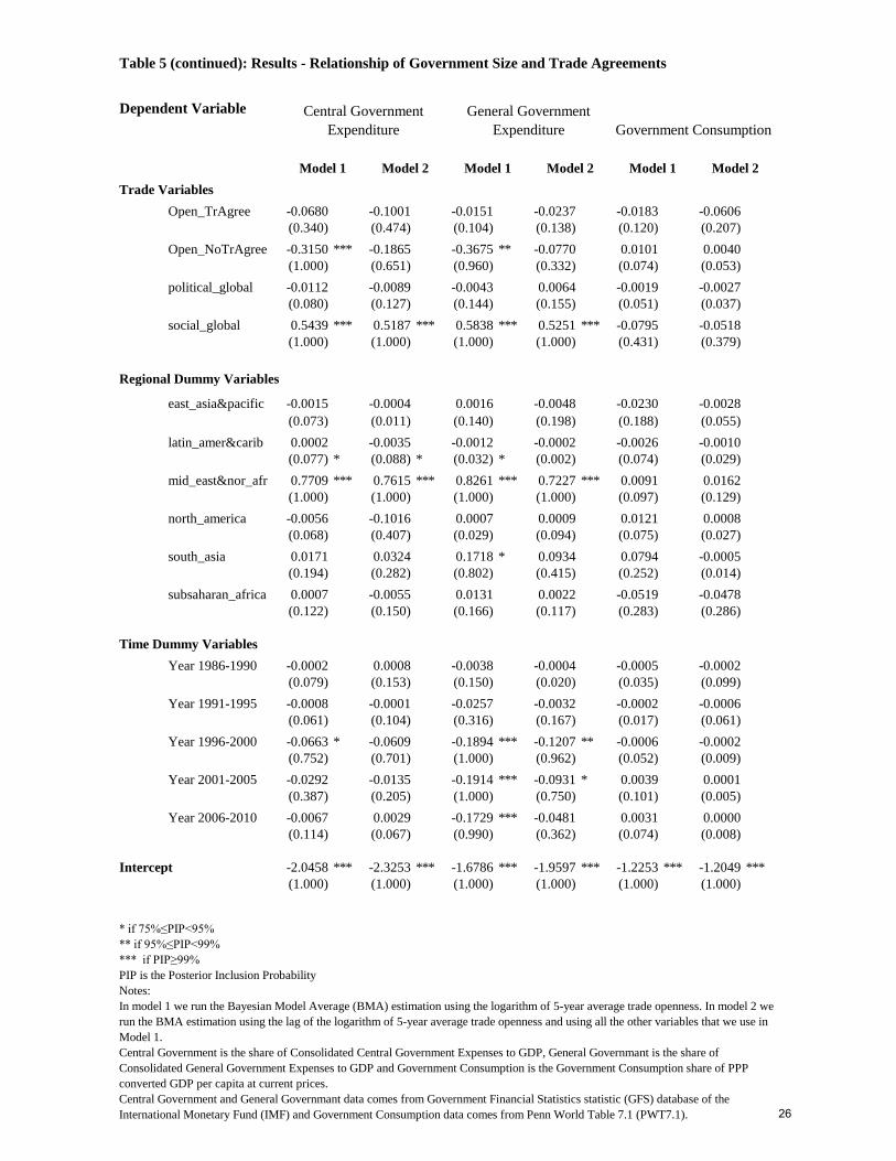
4.2. Relationship of Government Size and Trade Agreements
In Table 5 we can see the variables that affect the three government size dependent variables. Those models
use the exact same control variables as the Table 4. The only difference is that we do not use the trade
openness variable. We instead use the two trade openness variables that we constructed: Trade openness
under the trade agreement regime and Trade openness under no trade agreement regime. We want to check if
the use of those new variables affects the coefficients of the control variables and if by using those variables
we have new information about the relationship between trade openness and government expenditures. The
Trade openness under the trade agreement regime has very low PIP for all government size variables, for all
models, showing evidence against the effect according to Kass and Raftery (1995). Those result do not
support neither the compensate nor the efficiency hypothesis, and we can state that the trade with a country
under a trade agreement (Customs Union, Economic Integration Agreement, Free Trade Agreement and
Partial Scope Agreement) does not affect government expenditures.
The Trade openness under no trade agreement regime has a negative sign when we use government
consumption as the dependent variable. PIP for the contemporaneous model (Model 1), when the central
government expenditure is used, is equal to 1 showing very strong evidence for the effect. When we use
general government expenditure for Model 1, PIP is equal to 0.96 showing strong evidence for the effect.
PIP for the first lag model (Model 2), when the central government expenditure is used, is equal to 0.651
showing positive evidence for the effect. When we use general government expenditure for Model 2, PIP is
equal to 0.332 showing evidence against for the effect. On the other hand, for both model when government
consumption is used as the dependent variable, we have a fairly low PIP, ranging from 0.053-0.074, showing
evidence against the effect. The results for the government expenditure are consistent with the efficiency
hypothesis and shows that the trade with a country with no trade agreements decreases government
expenditures.
Conflict Variables:
The Ethnic and Revolutionary wars dummies have a very low PIP for all government size variables, for all
models. For the government expenditure variables those results are the same as in the case where we use
trade openness. For the government consumption variable the results are different from the case where we
use trade openness, where we found very strong or strong evidence for the effect. Now the coefficient for
both models fall, and according to PIP we have a positive evidence for the effect.
23

Conflict Variables
ethnic_wars 0.0004 0.0002 0.0022 0.0064 0.1181 0.1241
(0.136) (0.004) (0.063) (0.105) (0.613) (0.636)
revol_wars -0.0017 -0.0006 0.0002 0.0004 -0.1223 -0.0581
(0.116) (0.101) (0.033) (0.018) (0.574) (0.287)
Demographic Variables
death_rate 0.4910 *** 0.4894 *** 0.4416 *** 0.4774 *** 0.0207 0.0631
(1.000) (1.000) (1.000) (1.000) (0.150) (0.380)
inf_morta_rate -0.2451 *** -0.2256 ** -0.2721 *** -0.2488 *** 0.0559 0.0160
(0.999) (0.953) (1.000) (1.000) (0.463) (0.174)
life_expect 0.0331 0.0207 -0.0187 0.0093 -0.0229 -0.0593
(0.116) (0.059) (0.095) (0.145) (0.094) (0.102)
pop_density 0.0000 -0.0009 -0.0005 -0.0041 3.6147 *** 3.5195 ***
(0.035) (0.083) (0.056) (0.169) (1.000) (1.000)
pop_growth -0.1258 -1.3554 -0.7239 -1.1752 0.0550 -0.0423
(0.082) (0.300) (0.175) (0.278) (0.049) (0.019)
population -0.0002 -0.0003 -0.0003 0.0017 -3.6442 *** -3.5558 ***
(0.029) (0.098) (0.051) (0.117) (1.000) (1.000)
urb_pop_growth -0.3108 -0.3452 -0.3099 -1.1232 0.1696 0.0251
(0.191) (0.144) (0.149) (0.320) (0.089) (0.034)
work_age_rat -0.0038 0.0013 0.0062 0.0143 0.0386 0.0255
(0.098) (0.085) (0.055) (0.155) (0.146) (0.146)
Geographic Variables
ethnic_fraction -0.0026 -0.0008 -0.0004 -0.0022 0.0056 0.0544 *
(0.116) (0.046) (0.041) (0.065) (0.100) (0.785)
lingu_fraction -0.0061 -0.0114 -0.0045 -0.0170 0.0009 -0.0001
(0.245) (0.457) (0.192) (0.530) (0.043) (0.085)
relig_fraction 0.0331 0.0348 0.0382 0.0219 0.0946 *** 0.0912 ***
(0.662) (0.664) (0.709) (0.450) (1.000) (1.000)
num_neighb_st 0.0456 *** 0.0473 *** 0.0408 *** 0.0487 ***
(1.000) (1.000) (1.000) (1.000)
total_area -0.0002 0.0006 0.0021 0.0095 3.6084 *** 3.5175 ***
(0.036) (0.042) (0.116) (0.393) (1.000) (1.000)
Economic Institution Variables
civil_liberties -0.0633 -0.0402 -0.0695 -0.1012 0.0000 0.0012
(0.420) (0.305) (0.495) (0.616) (0.038) (0.080)
Model 1 Model 2
Dependent Variable Central Government
Expenditure
Table 5 : Results - Relationship of Government Size and Trade Agreements
Model 1 Model 2
General Government
Expenditure
Model 1 Model 2
Government Consumption
24
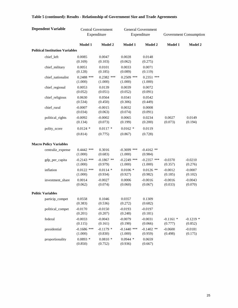
Political Institution Variables
chief_left 0.0085 0.0047 0.0028 0.0148
(0.169) (0.103) (0.062) (0.275)
chief_military 0.0051 0.0101 0.0033 0.0071
(0.128) (0.185) (0.089) (0.119)
chief_nationalist 0.2488 *** 0.2382 *** 0.2509 *** 0.2351 ***
(1.000) (1.000) (1.000) (1.000)
chief_regional 0.0053 0.0139 0.0039 0.0072
(0.052) (0.051) (0.052) (0.091)
chief_religious 0.0630 0.0564 0.0341 0.0542
(0.534) (0.450) (0.306) (0.449)
chief_rural -0.0007 -0.0015 0.0032 0.0008
(0.034) (0.063) (0.074) (0.091)
political_rights -0.0092 -0.0002 0.0065 0.0234 0.0027 0.0149
(0.134) (0.073) (0.199) (0.200) (0.073) (0.194)
polity_score 0.0124 * 0.0117 * 0.0162 * 0.0119
(0.814) (0.775) (0.867) (0.728)
Macro Policy Variables
centraliz_expense 0.4442 *** 0.3016 -0.3699 *** -0.4162 **
(1.000) (0.683) (1.000) (0.984)
gdp_per_capita -0.2143 *** -0.1867 ** -0.2249 *** -0.2357 *** -0.0370 -0.0210
(1.000) (0.979) (1.000) (1.000) (0.357) (0.276)
inflation 0.0122 *** 0.0114 * 0.0106 * 0.0126 ** -0.0012 -0.0007
(1.000) (0.934) (0.927) (0.982) (0.185) (0.102)
investment_share 0.0014 -0.0027 0.0006 -0.0016 -0.0016 -0.0043
(0.062) (0.074) (0.060) (0.067) (0.033) (0.070)
Politic Variables
particip_compet 0.0558 0.1046 0.0357 0.1309
(0.383) (0.536) (0.272) (0.682)
political_compet -0.0170 -0.0150 -0.0193 -0.0197
(0.201) (0.207) (0.248) (0.181)
federal -0.0033 -0.0043 -0.0079 -0.0031 -0.1161 * -0.1219 *
(0.115) (0.161) (0.190) (0.066) (0.777) (0.852)
presidential -0.1686 *** -0.1179 * -0.1440 *** -0.1402 ** -0.0600 -0.0181
(1.000) (0.830) (1.000) (0.959) (0.498) (0.175)
proportionality 0.0893 * 0.0810 * 0.0944 * 0.0659
(0.850) (0.752) (0.936) (0.667)
Table 5 (continued): Results - Relationship of Government Size and Trade Agreements
Dependent Variable Central Government
Expenditure
General Government
Expenditure Government Consumption
Model 1 Model 2 Model 1 Model 2 Model 1 Model 2
25
Trade Variables
Open_TrAgree -0.0680 -0.1001 -0.0151 -0.0237 -0.0183 -0.0606
(0.340) (0.474) (0.104) (0.138) (0.120) (0.207)
Open_NoTrAgree -0.3150 *** -0.1865 -0.3675 ** -0.0770 0.0101 0.0040
(1.000) (0.651) (0.960) (0.332) (0.074) (0.053)
political_global -0.0112 -0.0089 -0.0043 0.0064 -0.0019 -0.0027
(0.080) (0.127) (0.144) (0.155) (0.051) (0.037)
social_global 0.5439 *** 0.5187 *** 0.5838 *** 0.5251 *** -0.0795 -0.0518
(1.000) (1.000) (1.000) (1.000) (0.431) (0.379)
Regional Dummy Variables
east_asia&pacific -0.0015 -0.0004 0.0016 -0.0048 -0.0230 -0.0028
(0.073) (0.011) (0.140) (0.198) (0.188) (0.055)
latin_amer&carib 0.0002 -0.0035 -0.0012 -0.0002 -0.0026 -0.0010
(0.077) * (0.088) * (0.032) * (0.002) (0.074) (0.029)
mid_east&nor_afr 0.7709 *** 0.7615 *** 0.8261 *** 0.7227 *** 0.0091 0.0162
(1.000) (1.000) (1.000) (1.000) (0.097) (0.129)
north_america -0.0056 -0.1016 0.0007 0.0009 0.0121 0.0008
(0.068) (0.407) (0.029) (0.094) (0.075) (0.027)
south_asia 0.0171 0.0324 0.1718 * 0.0934 0.0794 -0.0005
(0.194) (0.282) (0.802) (0.415) (0.252) (0.014)
subsaharan_africa 0.0007 -0.0055 0.0131 0.0022 -0.0519 -0.0478
(0.122) (0.150) (0.166) (0.117) (0.283) (0.286)
Time Dummy Variables
Year 1986-1990 -0.0002 0.0008 -0.0038 -0.0004 -0.0005 -0.0002
(0.079) (0.153) (0.150) (0.020) (0.035) (0.099)
Year 1991-1995 -0.0008 -0.0001 -0.0257 -0.0032 -0.0002 -0.0006
(0.061) (0.104) (0.316) (0.167) (0.017) (0.061)
Year 1996-2000 -0.0663 * -0.0609 -0.1894 *** -0.1207 ** -0.0006 -0.0002
(0.752) (0.701) (1.000) (0.962) (0.052) (0.009)
Year 2001-2005 -0.0292 -0.0135 -0.1914 *** -0.0931 * 0.0039 0.0001
(0.387) (0.205) (1.000) (0.750) (0.101) (0.005)
Year 2006-2010 -0.0067 0.0029 -0.1729 *** -0.0481 0.0031 0.0000
(0.114) (0.067) (0.990) (0.362) (0.074) (0.008)
Intercept -2.0458 *** -2.3253 *** -1.6786 *** -1.9597 *** -1.2253 *** -1.2049 ***
(1.000) (1.000) (1.000) (1.000) (1.000) (1.000)
* if 75%≤PIP<95%
** if 95%≤PIP<99%
*** if PIP≥99%
PIP is the Posterior Inclusion Probability
Notes:
In model 1 we run the Bayesian Model Average (BMA) estimation using the logarithm of 5-year average trade openness. In model 2 we
run the BMA estimation using the lag of the logarithm of 5-year average trade openness and using all the other variables that we use in
Model 1.
Central Government is the share of Consolidated Central Government Expenses to GDP, General Governmant is the share of
Consolidated General Government Expenses to GDP and Government Consumption is the Government Consumption share of PPP
converted GDP per capita at current prices.
Central Government and General Governmant data comes from Government Financial Statistics statistic (GFS) database of the
International Monetary Fund (IMF) and Government Consumption data comes from Penn World Table 7.1 (PWT7.1).
Table 5 (continued): Results - Relationship of Government Size and Trade Agreements
Dependent Variable Central Government
Expenditure
General Government
Expenditure Government Consumption
Model 1 Model 2 Model 1 Model 2 Model 1 Model 2
26

Demographic Variables:
Death rate has a positive effect on all government expenditure variables as in the case where we use trade
openness. In all model the PIP is equal to 1, showing very strong evidence for the effect. For government
consumption PIP is very low, as before, showing evidence against the effect.
Infant mortality rate has a negative effect on all government expenditure variables as in the case where we
use trade openness. PIP is ranging from 0.953-1 in every of those models, showing strong or very strong
evidence for the effect. This is not true if we use the government consumption as the dependent variable,
where, as before, PIP shows evidence against the effect.
Life expectancy has a fairly low PIP, showing evidence against the effect, for all government size variables.
The overall results are quite similar as in the case where we use trade openness.
Population density has a very strong positive effect only when the government consumption is used as the
dependent variable. For government expenditure we have evidence against the effect. The overall results are
quite similar as in the case where we use trade openness.
Population growth has a very low PIP for all government size variables showing evidence against the effect.
The overall results are quite similar as in the case where we use trade openness.
Population has a negative effect only when we use government consumption. PIP is equal to 1showing very
strong evidence for the effect. When we use government expenditure we have evidence against the effect.
The overall results are quite similar as in the case where we use trade openness.
Both urban population growth and working age ratio have a fairly low PIP, for all government size variables,
showing evidence against the effect. The overall results are quite similar as in the case where we use trade
openness.
Geographic Variables:
The overall results for Ethnic, Linguistic and Religious fractionalization index are quite similar as in the case
where we use trade openness. The Ethnic, Linguistic and Religious fractionalization index have very a low
PIP for all government size variables, for all models, showing evidence against the effect according to Kass
and Raftery (1995) as in the case where we use trade openness. As before the only exception is when we use
the religious fractionalization index on government consumption, where it has a very strong positive effect.
The only difference from the case where we use trade openness is the ethnic fractionalization index, for the
first lag model (Model 2), when the dependent variable is government consumption. PIP is 0.785 showing a
positive evidence for the effect.
The number of neighboring states sharing a border with the identified state has a positive effect on all
government expenditure variables as in the case where we use trade openness. PIP is ranging from 0.973-1
in all of those models, showing strong or very strong evidence for the effect. The overall results are quite
similar as in the case where we use trade openness.
The country’s total area in square kilometers has a very strong negative effect only for government
consumption. The overall results are quite similar as in the case where we use trade openness.
Economic Institution Variables:
27

The Civil liberties index has a fairly low PIP for all government size variables showing evidence against the
effect. When the dependent variable is general government, for the first lag model (Model 2), PIP is 0.616
showing a weak evidence for the effect. The overall results are quite similar as in the case where we use
trade openness.
Political Institution Variables:
The orientation of the chief executive party (in our case if we test for a left party), has a very low PIP for all
government expenditures variables, for all models, showing evidence against the effect according to Kass
and Raftery (1995) as in the case where we use trade openness.
The results show that a chief executive, who is a military officer, will not affect government expenditures.
PIP is ranging from 0.089-0.185, showing evidence against the effect. The overall results are quite similar as
in the case where we use trade openness.
The background of the chief executive party (we test for nationalist, regional, religious and rural parties) do
not seem to affect government expenditure, with the exception of a nationalist party, as in the case where we
use trade openness. If the chief executive party is nationalist then this affect positive all government
expenditure variables. The overall results are quite similar as in the case where we use trade openness.
The Political rights index has a fairly low PIP for all government size variables showing evidence against the
effect. The overall results are quite similar as in the case where we use trade openness.
The Revised combined polity score has quite similar results as in the case where we use trade openness. PIP
is ranging from 0.775-0.867 showing a positive evidence for the effect when we use the government
expenditure as the dependent variable. The only exception is for the first lag model (Model 2), for the
general government consumption
Macro Policy Variables:
The share of central government to general government expenditure has a strong or a very strong effect on
both government expenditure variables. PIP is ranging from 0.984-1 showing strong or very strong evidence
for the effect. This is not true for the first lag estimation (Model 2) on central government expenditure. For
central government expenditure we have a positive effect and for general government effect we have a
negative effect. The overall results are similar as in the case where we use trade openness.
Gdp per capita has a negative effect on both government expenditure variables as in the case where we use
trade openness. PIP is ranging from 0.979-1 in all of those models, showing strong or very strong evidence
for the effect. In contract with the case where we use trade openness, we have evidence against the effect of
GDP per capita on government consumption.
Inflation has a positive effect only for government expenditure. For central government expenditure, in the
contemporaneous estimation (Model 1) we have a very strong evidence for the effect and for the first lag
model (Model 2) we have a positive evidence for the effect. For general government expenditure, in Model 1
we have a positive evidence for the effect and in Model 1 we have a strong evidence for the effect. On the
other hand for government consumption we have evidence against the effect. The overall results are quite
similar as in the case where we use trade openness.
28

The share of investment to gdp has a very low PIP for all government size variables, for all models, showing
evidence against the effect according to Kass and Raftery (1995) as in the case where we use trade openness.
Politic Variables:
The Competitiveness of participation dummy, the Political competition index and the Federal system of
government have a very low PIP for all government size variables, for all models, showing evidence against
the effect according to Kass and Raftery (1995). This is not true for the federal system dummy only when
we use government consumption as the dependent variable where we have a positive evidence for the effect.
The overall results are similar as in the case where we use trade openness.
The Presidential type of regime has a negative effect on all government expenditure variables. PIP is ranging
from 0.830-1 in all of those models, showing positive, strong or very strong evidence for the effect. For the
government consumption variable the results are different from the case where we use trade openness, where
we found strong evidence for the effect. Now the coefficient for both models fall, and according to PIP we
have evidence against the effect.
The Proportional electoral rule has a positive effect on all government expenditure variables as in the case
where we use trade openness. Now the coefficient for both government expenditure variables fall and
according to Kass and Raftery (1995) rule of thumb there is a positive evidence for the effect. The overall
results are similar as in the case where we use trade openness.
Trade Variables:
The Political globalization index has a very low PIP for all government size variables, for all models,
showing evidence against the effect according to Kass and Raftery (1995). The overall results are similar as
in the case where we use trade openness.
The Social globalization index has a very strong, positive effect on all government expenditure variables. On
the other hand for government consumption we have evidence against the effect. The overall results are
similar as in the case where we use trade openness.
4.3. Robustness
In order to check the robustness of the results we run the models in tables 5 and 6 using four different
dependent variables. For government expenditure we use the hare of Consolidated Central Government
Total Outlays to GDP (GovExp2) and the share of Consolidated General Government Total Outlays to GDP
(GovExp4) from the Government Financial Statistics statistic (GFS) database of the International Monetary
Fund (IMF). Those two variables refer to the period 1972-2010, for 169 countries in an unbalanced panel.
For government consumption we use the Government Consumption share of PPP converted GDP per capita
at 2005 constant prices (GovCon2) from the Penn World Table 7.1 (PWT7.1) database and the share of
General Government Final Consumption Expenditure to GDP (GovCon3) from the World Development
Indicators (WDI) database of the World Bank (WB). GovCon2 refers to the period 1950-2010, for 147
countries in an unbalanced panel and GovCon3 refers to the period 1960-2011, for 185 countries in an
unbalanced panel. The results for the robustness check can be found in table 6 below.
29
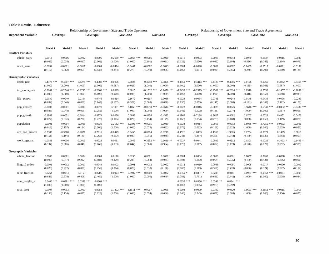
Conflict Variables
ethnic_wars 0.0013 0.0006 0.0002 0.0005 0.2659 *** 0.2664 *** 0.0066 0.0020 -0.0016 0.0003 0.0003 0.0044 0.1070 0.1537 0.0015 0.0037
(0.069) (0.035) (0.017) (0.062) (1.000) (1.000) (0.101) (0.031) (0.126) (0.050) (0.043) (0.104) (0.586) (0.745) (0.104) (0.076)
revol_wars -0.0054 -0.0021 -0.0017 -0.0004 -0.0494 -0.0467 -0.0062 -0.0043 -0.0004 -0.0028 -0.0002 0.0002 -0.0439 -0.0518 -0.0321 -0.0182
(0.117) (0.062) (0.061) (0.038) (0.284) (0.273) (0.090) (0.056) (0.009) (0.061) (0.036) (0.066) (0.248) (0.292) (0.250) (0.188)
Demographic Variables
death_rate 0.4378 *** 0.4507 *** 0.4278 *** 0.4780 *** -0.0006 -0.0024 0.3958 *** 0.3856 *** 0.4551 *** 0.4414 *** 0.4725 *** 0.4566 *** 0.0126 0.0066 0.3052 ** 0.3468 ***
(1.000) (1.000) (1.000) (1.000) (0.087) (0.026) (1.000) (1.000) (1.000) (1.000) (1.000) (1.000) (0.135) (0.063) (0.987) (1.000)
inf_morta_rate -0.2641 *** -0.2546 *** -0.2795 *** -0.2666 *** 0.0029 0.0015 -0.1532 *** -0.1470 *** -0.2432 *** -0.2379 *** -0.2562 *** -0.2616 *** 0.0310 0.0550 -0.1457 *** -0.1099 *
(1.000) (1.000) (1.000) (1.000) (0.060) (0.028) (1.000) (1.000) (1.000) (1.000) (1.000) (1.000) (0.318) (0.558) (0.998) (0.935)
life_expect -0.0030 -0.0040 0.0104 0.0746 0.0814 0.1679 -0.0257 -0.0088 0.0024 0.0054 0.0743 0.0248 -0.0148 -0.0435 -0.0408 -0.0239
(0.034) (0.040) (0.069) (0.143) (0.157) (0.322) (0.068) (0.038) (0.030) (0.055) (0.147) (0.080) (0.121) (0.169) (0.112) (0.103)
pop_density -0.0003 -0.0001 0.0000 -0.0070 3.1051 *** 3.1063 *** -0.0618 *** -0.0614 *** -0.0023 -0.0016 -0.0025 0.0026 3.5646 *** 3.6540 *** -0.0432 ** -0.0480 ***
(0.025) (0.048) (0.095) (0.252) (1.000) (1.000) (1.000) (1.000) (0.042) (0.122) (0.115) (0.277) (1.000) (1.000) (0.957) (0.996)
pop_growth -0.1883 -0.0031 -0.6814 -0.8774 0.0056 0.0059 -0.4356 -0.4552 -0.1869 -0.7138 -1.2627 -0.8082 0.0707 0.0028 0.4452 -0.0472
(0.077) (0.031) (0.230) (0.222) (0.015) (0.026) (0.154) (0.179) (0.065) (0.194) (0.273) (0.188) (0.068) (0.056) (0.119) (0.071)
population 0.0001 0.0004 0.0005 0.0039 -3.2182 *** -3.2193 *** 0.0005 0.0010 0.0024 0.0014 0.0013 -0.0013 -3.6056 *** -3.7055 *** -0.0003 -0.0006
(0.019) (0.157) (0.134) (0.200) (1.000) (1.000) (0.079) (0.092) (0.076) (0.092) (0.101) (0.322) (1.000) (1.000) (0.035) (0.051)
urb_pop_growth -0.2383 -0.3500 -0.2871 -0.7916 -0.0449 -0.0455 -0.0294 -0.0219 -0.4526 -1.0033 -1.1356 -1.9605 0.2754 -0.0079 0.1469 0.0816
(0.151) (0.191) (0.130) (0.262) (0.062) (0.037) (0.056) (0.048) (0.241) (0.317) (0.361) (0.544) (0.150) (0.030) (0.093) (0.053)
work_age_rat -0.0053 -0.0016 -0.0019 -0.0023 0.0031 0.0045 0.3552 ** 0.3689 ** -0.0027 -0.0041 0.0039 0.0212 0.0301 0.0029 0.3403 * 0.3495 *
(0.134) (0.085) (0.046) (0.068) (0.033) (0.044) (0.969) (0.964) (0.076) (0.117) (0.092) (0.173) (0.170) (0.027) (0.892) (0.905)
Geographic Variables
ethnic_fraction 0.0000 0.0001 0.0004 0.0004 0.0110 0.0136 0.0001 0.0002 -0.0004 0.0004 -0.0006 0.0001 0.0057 0.0260 -0.0008 0.0000
(0.000) (0.047) (0.222) (0.084) (0.229) (0.289) (0.084) (0.045) (0.104) (0.112) (0.054) (0.035) (0.160) (0.431) (0.056) (0.006)
lingu_fraction -0.0001 -0.0012 -0.0017 -0.0049 -0.0003 -0.0001 -0.0002 -0.0002 -0.0012 -0.0010 -0.0086 -0.0091 0.0008 0.0017 0.0000 -0.0002
(0.020) (0.222) (0.097) (0.259) (0.014) (0.023) (0.033) (0.138) (0.108) (0.113) (0.367) (0.420) (0.036) (0.124) (0.027) (0.112)
relig_fraction 0.0264 0.0244 0.0153 0.0206 0.0923 *** 0.0902 *** 0.0000 0.0002 0.0359 * 0.0391 * 0.0283 0.0181 0.0937 *** 0.0952 *** -0.0004 -0.0003
(0.648) (0.578) (0.408) (0.460) (1.000) (1.000) (0.000) (0.049) (0.783) (0.781) (0.631) (0.442) (1.000) (1.000) (0.038) (0.084)
num_neighb_st 0.0400 *** 0.0381 *** 0.0389 *** 0.0364 *** 0.0355 *** 0.0356 *** 0.0349 ** 0.0341 ***
(1.000) (1.000) (1.000) (1.000) (1.000) (0.995) (0.973) (0.992)
total_area 0.0004 0.0013 0.0000 0.0058 3.1492 *** 3.1511 *** 0.0007 0.0001 0.0003 0.0079 0.0199 0.0320 3.5693 *** 3.6652 *** 0.0015 0.0013
(0.153) (0.134) (0.027) (0.223) (1.000) (1.000) (0.054) (0.006) (0.146) (0.243) (0.658) (0.688) (1.000) (1.000) (0.136) (0.055)
Table 6: Results - Robustness
Model 1 Model 2
GovCon2
Model 1 Model 2
GovCon3
Model 2
GovExp2
Relationship of Government Size and Trade Openness
Model 1 Model 2
GovExp4
Relationship of Government Size and Trade Agreements
Model 1 Model 2Model 1 Model 2
GovExp2
Model 1
Dependent Variable GovCon3
Model 1Model 2
GovExp4
Model 1 Model 2
GovCon2
30
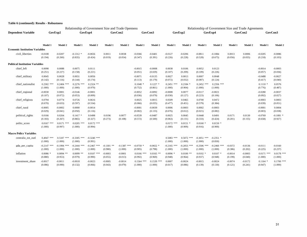
Economic Institution Variables
civil_liberties -0.0108 -0.0207 -0.1312 * -0.0656 0.0011 0.0038 -0.0366 -0.0401 -0.0127 -0.0206 -0.0811 -0.1084 0.0013 0.0006 -0.0205 -0.0086
(0.194) (0.260) (0.835) (0.424) (0.019) (0.054) (0.347) (0.391) (0.226) (0.228) (0.528) (0.675) (0.056) (0.035) (0.218) (0.103)
Political Institution Variables
chief_left 0.0098 0.0088 0.0075 0.0111 -0.0015 -0.0008 0.0038 0.0106 0.0052 0.0123 -0.0014 -0.0003
(0.251) (0.227) (0.158) (0.221) (0.051) (0.029) (0.107) (0.209) (0.109) (0.226) (0.057) (0.036)
chief_military 0.0045 0.0028 0.0031 0.0056 -0.0071 -0.0135 0.0027 0.0013 0.0007 0.0048 -0.0488 -0.0027
(0.142) (0.116) (0.144) (0.174) (0.113) (0.179) (0.072) (0.032) (0.087) (0.124) (0.417) (0.040)
chief_nationalist 0.2302 *** 0.2404 *** 0.2276 *** 0.2324 ** 0.1048 * 0.1227 * 0.2451 *** 0.2184 * 0.2452 *** 0.2356 *** 0.1110 * 0.0576
(1.000) (1.000) (1.000) (0.979) (0.752) (0.861) (1.000) (0.904) (1.000) (1.000) (0.776) (0.487)
chief_regional -0.0030 0.0001 -0.0146 -0.0001 -0.0052 -0.0092 -0.0008 0.0077 -0.0117 -0.0021 -0.0280 -0.0037
(0.107) (0.072) (0.053) (0.009) (0.036) (0.079) (0.030) (0.127) (0.223) (0.106) (0.092) (0.027)
chief_religious 0.0794 0.0774 0.0726 0.0616 0.0025 0.0015 0.0509 0.0465 0.0700 0.0472 -0.0003 0.0003
(0.670) (0.633) (0.597) (0.534) (0.066) (0.035) (0.477) (0.451) (0.579) (0.384) (0.039) (0.051)
chief_rural -0.0005 -0.0002 0.0000 -0.0014 -0.0001 -0.0039 0.0006 -0.0003 0.0002 -0.0003 -0.0001 0.0004
(0.029) (0.041) (0.050) (0.116) (0.002) (0.133) (0.076) (0.012) (0.021) (0.082) (0.003) (0.038)
political_rights 0.0166 0.0264 0.1417 * 0.0498 0.0196 0.0077 -0.0539 -0.0487 0.0025 0.0045 0.0448 0.0491 0.0171 0.0130 -0.0769 -0.1081 *
(0.183) (0.267) (0.865) (0.327) (0.273) (0.108) (0.572) (0.500) (0.063) (0.131) (0.333) (0.424) (0.201) (0.155) (0.658) (0.927)
polity_score 0.0167 *** 0.0171 *** 0.0205 *** 0.0172 *** 0.0172 *** 0.0151 * 0.0160 * 0.0150 *
(1.000) (0.997) (1.000) (0.994) (1.000) (0.909) (0.916) (0.900)
Macro Policy Variables
centraliz_tot_outl 0.4947 *** 0.5107 *** -0.3305 *** -0.3240 *** 0.5083 *** 0.5072 *** -0.3051 *** -0.2351 *
(1.000) (1.000) (1.000) (0.991) (1.000) (1.000) (1.000) (0.830)
gdp_per_capita -0.2147 *** -0.1994 *** -0.2444 *** -0.2467 *** -0.1301 ** -0.1387 *** -0.0759 * -0.0652 * -0.2165 *** -0.2053 *** -0.2506 *** -0.2460 *** -0.0372 -0.0136 -0.0111 -0.0160
(1.000) (1.000) (1.000) (1.000) (0.980) (1.000) (0.905) (0.798) (1.000) (1.000) (1.000) (1.000) (0.386) (0.202) (0.225) (0.237)
inflation 0.0086 * 0.0094 ** 0.0099 ** 0.0107 *** -0.0003 -0.0001 0.0166 *** 0.0165 ** 0.0096 * 0.0100 ** 0.0102 * 0.0107 * -0.0014 -0.0003 0.0171 *** 0.0178 ***
(0.880) (0.953) (0.979) (0.990) (0.055) (0.013) (0.992) (0.969) (0.948) (0.964) (0.937) (0.948) (0.199) (0.040) (1.000) (1.000)
investment_share -0.0017 -0.0011 -0.0018 -0.0023 -0.0005 -0.0014 0.1564 *** 0.1539 *** 0.0007 -0.0024 -0.0015 -0.0024 -0.0074 -0.0172 0.1164 * 0.1700 ***
(0.086) (0.090) (0.132) (0.066) (0.043) (0.079) (1.000) (1.000) (0.017) (0.086) (0.139) (0.130) (0.121) (0.241) (0.947) (1.000)
Model 2 Model 1 Model 2Model 1 Model 2 Model 1 Model 2 Model 1
Table 6 (continued): Results - Robustness
Relationship of Government Size and Trade Openness Relationship of Government Size and Trade Agreements
Dependent Variable GovExp2 GovExp4 GovCon2 GovCon3 GovExp2 GovExp4 GovCon2 GovCon3
Model 2Model 1 Model 2 Model 1 Model 2 Model 1Model 2 Model 1
31
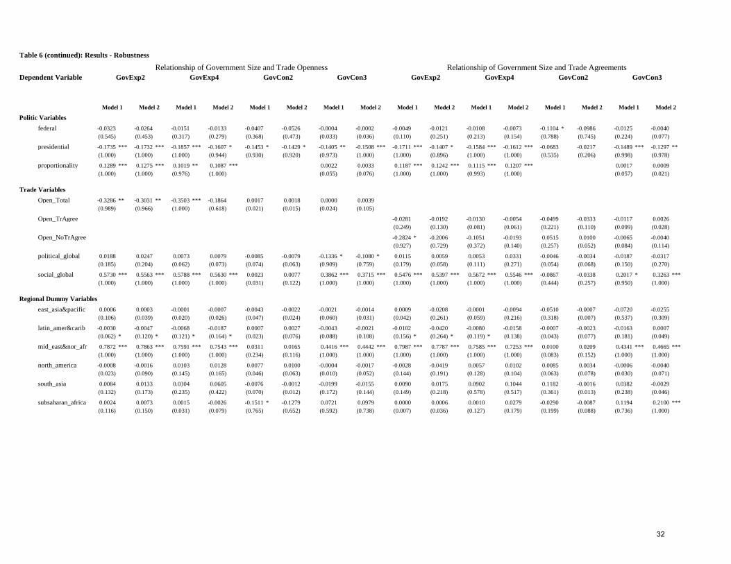
Politic Variables
federal -0.0323 -0.0264 -0.0151 -0.0133 -0.0407 -0.0526 -0.0004 -0.0002 -0.0049 -0.0121 -0.0108 -0.0073 -0.1104 * -0.0986 -0.0125 -0.0040
(0.545) (0.453) (0.317) (0.279) (0.368) (0.473) (0.033) (0.036) (0.110) (0.251) (0.213) (0.154) (0.788) (0.745) (0.224) (0.077)
presidential -0.1735 *** -0.1732 *** -0.1857 *** -0.1607 * -0.1453 * -0.1429 * -0.1405 ** -0.1508 *** -0.1711 *** -0.1407 * -0.1584 *** -0.1612 *** -0.0683 -0.0217 -0.1489 *** -0.1297 **
(1.000) (1.000) (1.000) (0.944) (0.930) (0.920) (0.973) (1.000) (1.000) (0.896) (1.000) (1.000) (0.535) (0.206) (0.998) (0.978)
proportionality 0.1289 *** 0.1275 *** 0.1019 ** 0.1087 *** 0.0022 0.0033 0.1187 *** 0.1242 *** 0.1115 *** 0.1207 *** 0.0017 0.0009
(1.000) (1.000) (0.976) (1.000) (0.055) (0.076) (1.000) (1.000) (0.993) (1.000) (0.057) (0.021)
Trade Variables
Open_Total -0.3286 ** -0.3031 ** -0.3503 *** -0.1864 0.0017 0.0018 0.0000 0.0039
(0.989) (0.966) (1.000) (0.618) (0.021) (0.015) (0.024) (0.105)
Open_TrAgree -0.0281 -0.0192 -0.0130 -0.0054 -0.0499 -0.0333 -0.0117 0.0026
(0.249) (0.130) (0.081) (0.061) (0.221) (0.110) (0.099) (0.028)
Open_NoTrAgree -0.2824 * -0.2006 -0.1051 -0.0193 0.0515 0.0100 -0.0065 -0.0040
(0.927) (0.729) (0.372) (0.140) (0.257) (0.052) (0.084) (0.114)
political_global 0.0188 0.0247 0.0073 0.0079 -0.0085 -0.0079 -0.1336 * -0.1080 * 0.0115 0.0059 0.0053 0.0331 -0.0046 -0.0034 -0.0187 -0.0317
(0.185) (0.204) (0.062) (0.073) (0.074) (0.063) (0.909) (0.759) (0.179) (0.058) (0.111) (0.271) (0.054) (0.068) (0.150) (0.270)
social_global 0.5730 *** 0.5563 *** 0.5788 *** 0.5630 *** 0.0023 0.0077 0.3862 *** 0.3715 *** 0.5476 *** 0.5397 *** 0.5672 *** 0.5546 *** -0.0867 -0.0338 0.2017 * 0.3263 ***
(1.000) (1.000) (1.000) (1.000) (0.031) (0.122) (1.000) (1.000) (1.000) (1.000) (1.000) (1.000) (0.444) (0.257) (0.950) (1.000)
Regional Dummy Variables
east_asia&pacific 0.0006 0.0003 -0.0001 -0.0007 -0.0043 -0.0022 -0.0021 -0.0014 0.0009 -0.0208 -0.0001 -0.0094 -0.0510 -0.0007 -0.0720 -0.0255
(0.106) (0.039) (0.020) (0.026) (0.047) (0.024) (0.060) (0.031) (0.042) (0.261) (0.059) (0.216) (0.318) (0.007) (0.537) (0.309)
latin_amer&carib -0.0030 -0.0047 -0.0068 -0.0187 0.0007 0.0027 -0.0043 -0.0021 -0.0102 -0.0420 -0.0080 -0.0158 -0.0007 -0.0023 -0.0163 0.0007
(0.062) * (0.120) * (0.121) * (0.164) * (0.023) (0.076) (0.088) (0.108) (0.156) * (0.264) * (0.119) * (0.138) (0.043) (0.077) (0.181) (0.049)
mid_east&nor_afr 0.7872 *** 0.7863 *** 0.7591 *** 0.7543 *** 0.0311 0.0165 0.4416 *** 0.4442 *** 0.7987 *** 0.7787 *** 0.7585 *** 0.7253 *** 0.0100 0.0209 0.4341 *** 0.4665 ***
(1.000) (1.000) (1.000) (1.000) (0.234) (0.116) (1.000) (1.000) (1.000) (1.000) (1.000) (1.000) (0.083) (0.152) (1.000) (1.000)
north_america -0.0008 -0.0016 0.0103 0.0128 0.0077 0.0100 -0.0004 -0.0017 -0.0028 -0.0419 0.0057 0.0102 0.0085 0.0034 -0.0006 -0.0040
(0.023) (0.090) (0.145) (0.165) (0.046) (0.063) (0.010) (0.052) (0.144) (0.191) (0.128) (0.104) (0.063) (0.078) (0.030) (0.071)
south_asia 0.0084 0.0133 0.0304 0.0605 -0.0076 -0.0012 -0.0199 -0.0155 0.0090 0.0175 0.0902 0.1044 0.1182 -0.0016 0.0382 -0.0029
(0.132) (0.173) (0.235) (0.422) (0.070) (0.012) (0.172) (0.144) (0.149) (0.218) (0.578) (0.517) (0.361) (0.013) (0.238) (0.046)
subsaharan_africa 0.0024 0.0073 0.0015 -0.0026 -0.1511 * -0.1279 0.0721 0.0979 0.0000 0.0006 0.0010 0.0279 -0.0290 -0.0087 0.1194 0.2100 ***
(0.116) (0.150) (0.031) (0.079) (0.765) (0.652) (0.592) (0.738) (0.007) (0.036) (0.127) (0.179) (0.199) (0.088) (0.736) (1.000)
Model 2 Model 1 Model 2 Model 1
Table 6 (continued): Results - Robustness
Relationship of Government Size and Trade Openness Relationship of Government Size and Trade Agreements
Dependent Variable GovExp2 GovExp4 GovCon2 GovCon3 GovExp2 GovExp4 GovCon2 GovCon3
Model 2Model 1 Model 2 Model 1 Model 2 Model 1Model 2 Model 1 Model 2 Model 1 Model 2Model 1
32
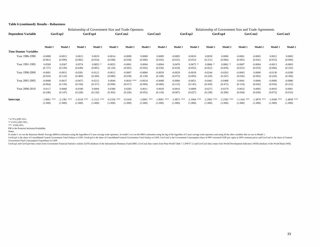
Time Dummy Variables
Year 1986-1990 -0.0008 -0.0013 0.0015 0.0019 -0.0014 -0.0009 0.0000 0.0009 -0.0005 -0.0010 0.0039 0.0000 -0.0001 -0.0002 0.0012 0.0002
(0.061) (0.099) (0.082) (0.054) (0.048) (0.028) (0.000) (0.043) (0.025) (0.053) (0.221) (0.066) (0.005) (0.041) (0.053) (0.006)
Year 1991-1995 0.0509 0.0367 0.0574 0.0853 * -0.0053 -0.0001 0.0004 0.0004 0.0476 0.0675 * 0.0866 * 0.0862 * -0.0007 -0.0004 -0.0013 -0.0003
(0.727) (0.539) (0.649) (0.891) (0.120) (0.002) (0.043) (0.036) (0.618) (0.835) (0.822) (0.839) (0.022) (0.019) (0.066) (0.102)
Year 1996-2000 -0.0001 -0.0031 -0.0281 -0.0121 -0.0012 -0.0007 -0.0084 -0.0059 -0.0029 -0.0018 -0.0244 -0.0263 -0.0003 0.0000 -0.0130 -0.0189
(0.010) (0.110) (0.400) (0.260) (0.080) (0.039) (0.139) (0.108) (0.072) (0.093) (0.229) (0.247) (0.026) (0.002) (0.243) (0.306)
Year 2001-2005 -0.0008 -0.0037 -0.0475 -0.0212 0.0044 0.0010 *** -0.0024 -0.0008 -0.0060 -0.0051 -0.0445 -0.0488 0.0041 0.0006 -0.0006 -0.0086
(0.064) (0.120) (0.556) (0.317) (0.090) (0.017) (0.069) (0.060) (0.123) (0.145) (0.429) (0.472) (0.124) (0.042) (0.026) (0.222)
Year 2006-2010 0.0117 0.0060 -0.0180 0.0004 0.0380 0.0283 0.0011 0.0029 -0.0010 0.0009 -0.0275 -0.0279 0.0032 0.0005 -0.0010 -0.0001
(0.246) (0.147) (0.228) (0.120) (0.302) (0.226) (0.052) (0.118) (0.067) (0.027) (0.238) (0.296) (0.044) (0.020) (0.072) (0.033)
Intercept -1.9661 *** -2.1381 *** -1.6518 *** -2.1512 *** -0.2336 *** -0.5418 -1.6901 *** -1.9091 *** -1.9875 *** -2.1064 *** -2.2902 *** -2.2583 *** -1.1104 *** -1.3879 *** -1.9349 *** -2.4858 ***
(1.000) (1.000) (1.000) (1.000) (1.000) (1.000) (1.000) (1.000) (1.000) (1.000) (1.000) (1.000) (1.000) (1.000) (1.000) (1.000)
Table 6 (continued): Results - Robustness
Relationship of Government Size and Trade Openness Relationship of Government Size and Trade Agreements
Dependent Variable GovExp2 GovExp4 GovCon2 GovCon3 GovExp2 GovExp4 GovCon2 GovCon3
Model 2
* if 75%≤PIP<95%
** if 95%≤PIP<99%
*** if PIP≥99%
PIP is the Posterior Inclusion Probability
Notes:
In model 1 we run the Bayesian Model Average (BMA) estimation using the logarithm of 5-year average trade openness. In model 2 we run the BMA estimation using the lag of the logarithm of 5-year average trade openness and using all the other variables that we use in Model 1.
GovExp2 is the share of Consolidated Central Government Total Outlays to GDP, GovExp4 is the share of Consolidated General Government Total Outlays to GDP, GovCon2 is the Government Consumption share of PPP converted GDP per capita at 2005 constant prices and GovCon3 is the share of General
Government Final Consumption Expenditure to GDP.
GovExp2 and GovExp4 data comes from Government Financial Statistics statistic (GFS) database of the International Monetary Fund (IMF), GovCon2 data comes from Penn World Table 7.1 (PWT7.1) and GovCon3 data comes from World Development Indicators (WDI) database of the World Bank (WB).
Model 1 Model 2 Model 1 Model 2 Model 1Model 2 Model 1 Model 2 Model 1 Model 2Model 1 Model 2 Model 1 Model 2 Model 1
33
Trade openness has a negative coefficient on both new government expenditure variables. PIP is ranging
from 0.966-1, showing strong or very strong evidence for the effect. The only exception is the first lag
model (Model 2) where PIP shows weak evidence for the effect. PIP shows evidence against the effect of
trade openness on both the new government consumption variables. Those results are robust with our
previous findings and consistent with the efficiency hypothesis.
For all new dependent variables, for all models, PIP for the trade openness under trade agreement regime is
less than 0.5, showing evidence against the effect. The Trade openness under no trade agreement regime has
a negative sign only on the new central government expenditure and PIP shows strong evidence for the
effect. The results for both trade openness variables, under trade agreement regime and under no trade
agreement regime, are robust with the previous ones.
Conflict Variables:
The Ethnic and Revolutionary wars dummies have a very low PIP for all government size variables, for all
models even if we use trade openness or trade openness with the trade agreement information. The only
exception, as in our previous finding, is the government consumption variable from PWT7.1 where we have
very strong evidence for a positive effect.
Demographic Variables:
Death rate has a positive effect on all government size variables, for all trade openness variables. PIP shows
strong or very strong evidence for the effect. The only exception is when we use the government
consumption from PWT7.1, where we have evidence against the effect if we use trade openness and weak
evidence for the effect if we use trade openness under trade agreement regime. The overall results are robust
with our previous findings.
Infant mortality rate has a negative effect on all government size variables, for all trade openness variables.
PIP shows strong or very strong evidence for the effect. The only exception is when we use the government
consumption from PWT7.1, where we have evidence against the effect if we use trade openness and weak
evidence for the effect if we use trade openness under trade agreement regime. The overall results are robust
with our previous findings.
Life expectancy has a fairly low PIP, showing evidence against the effect, for all government size variables,
for all trade openness variables. The overall results are quite similar with our previous results.
The PIP of the population density shows very strong evidence for the effect only on the government
consumption variable. We found a positive effect on the government consumption from PWT7.1 and a
negative effect on the government consumption from WDI.
Population growth has a fairly low PIP, showing evidence against the effect, for all government size
variables, for all trade openness variables. The overall results are robust with our previous findings.
Population has a negative effect only when we use government consumption from PWT7.1. PIP shows very
strong evidence for the effect. The overall results are robust with our previous results.
Both urban population growth and working age ratio have a fairly low PIP, for all government size variables,
for all trade openness variables. Those results are robust with our previous finding. The only exception is the
34

positive effect on the government consumption from WDI of the working age ratio. PIP shows strong
evidence using either the trade openness variable or the trade agreement openness.
Geographic Variables:
The overall results for Ethnic, Linguistic and Religious fractionalization index are robust with our previous
results. The Ethnic, Linguistic and Religious fractionalization index have very a low PIP for all government
size variables, for all models, for all trade openness variables. The only difference is the religious
fractionalization index, when the dependent variable is government consumption from PWT7.1 where we
have a very strong evidence for the effect. Also we have a positive evidence for the effect for the religious
fractionalization index, when we use the trade agreement variables.
The number of neighboring states sharing a border with the identified state has a strong or very strong
evidence for a positive effect on all new government expenditure variables, showing robustness with our
previous finding.
The country’s total area in square kilometers has a very strong negative effect only for government
consumption as before. The overall results are robust with the previous ones.
Economic Institution Variables:
The Civil liberties index has a fairly low PIP for all new government size variables, for all models, for all
trade openness variables. Those results are robust with our previous findings.
Political Institution Variables:
The orientation of the chief executive party (in our case if we test for a left party), has a very low PIP for all
new government size variables, for all models, for all trade openness variables showing robustness with our
previous results.
The results show that a chief executive, who is a military officer, will affect none of the new government
size variables. We get the same results with our previous findings.
The results from the background of the chief executive party (we test for nationalist, regional, religious and
rural parties) on the new government size variables are robust with our previous findings. As before if the
chief executive party is nationalist then this affect positive all government expenditure variables.
The Political rights index has a very low PIP for all new government size variables, for all models, for all
trade openness variables showing robustness with our previous results.
The Revised combined polity score has very strong evidence for a positive effect on both the new
government expenditure variables. Those results are robust with our previous findings.
Macro Policy Variables:
The share of central government to general government expenditure has a strong or a very strong effect on
both the new government expenditure variables. As before for the central government expenditure we have a
positive effect and for general government effect we have a negative effect.
Gdp per capita has a negative effect on all new government size variables when we use the trade openness
variable and a negative effect on the government expenditure variables when we use the trade agreement
openness. Those results are robust with our previous findings.
35
Inflation has a positive effect on the two new government expenditure variables and on the government
consumption variable from WDI. For government expenditure we have strong evidence for the effect if we
use the trade openness variable and positive evidence for the effect if we use the trade agreement openness
variables. For government consumption we have very strong evidence for the effect for any trade openness
variable we use.
The share of investment to gdp has a very low PIP for all government size variables, for all models, showing
evidence against the effect. The only exception with our previous results is the very strong evidence for a
positive effect on the government consumption from WDI.
Politic Variables:
The Federal system of government has a very low PIP for all government size variables, for all trade
openness variables showing robustness with our previous results.
The Presidential type of regime has a negative effect on all government size variables. PIP shows very
strong evidence for the effect on the government expenditure and on government consumption from WDI
even if we use trade openness or trade openness with the trade agreement information. Those results are
robust with our previous findings.
The Proportional electoral rule has a positive effect only on the government expenditure. PIP shows very
strong evidence for the effect something which is robust with our previous findings.
Trade Variables:
The Political globalization index has a very low PIP for all government size variables, for all models, for all
trade openness variables showing robustness with our previous results.
The Social globalization index has a very strong, positive effect on all government size variables. The only
exception is when we use the government consumption variable from PWT7.1 as the dependent variable.
The overall results are robust with our previous findings.
36
5. Conclusion
Through this study we tried to find what the determinants of government size are. We used data for 102
countries from 1976 to 2010. Data for the dependent variables come from the Penn World Table 7.1
(PWT7.1) database and the Government Financial Statistics statistic (GFS) database of the International
Monetary Fund (IMF). Studying the existing literature we tried to use all possible control variables that
authors used in order to determine which of those affect government size. We tested more than 140
variables, and ended up with 45 for our final model. Control variables come from the Political Institutions
database, the Freedom House database, the KOF Index of Globalization database, the Polity IV database, the
Penn World Table 7.1 database, the Quality of Government Institute database, the World Development
Indicators database and the World Trade Organization database. In order to find the determinants of
government expenditures and consumption we used the Bayesian Model Average estimation so that to count
for model uncertainty.
Our main independent variable is trade openness. The most used measure of trade openness is the share of
the sum of exports and imports to gdp. We tested trade openness from various datasets and ended up with
the one from the Penn World Table 7.1, because it includes data for more countries than other datasets. The
relationship between government size and trade openness is not clear. This relationship divides the literature
into two hypotheses. The first one indicates that more open countries have greater government size
(compensate hypothesis) and the second one that more open countries have lower government size
(efficiency hypothesis).
We found that by using trade openness, the results for government expenditure are consistent with the
efficiency hypothesis. This shows that more trade open countries tend on average to decrease their
government expenditures. This is not true if we use government consumption. We found a statistically
insignificant coefficient which shows that trade does not affect government consumption. When we divide
trade openness into trade openness under the trade agreement regime and trade openness under no trade
agreement regime we get new information on how trade affects government size. For government
expenditure we found evidence that trade under customs union, economic integration agreements, free trade
agreements and partial scope agreements does not support neither the compensate nor the efficiency
hypothesis. This was something that we expected since the countries that signed those agreements agreed to
let trade between them free of any government intervention. On the other hand, we found evidence of a
negative relationship between trade under no trade agreement regime and government expenditure. This
shows that trade can be very beneficial for a country that wants to decrease its expenditure and achieve a
fiscal adjustment. Finally we found that neither trade openness under the trade agreement regime nor trade
openness under no trade agreement regime affect government consumption.
The main control variables that affect government expenditures are death rate, infant mortality rate, the
number of neighboring countries sharing a border, if the chief executive party is nationalist, the share of
central to general government expenditure, gdp per capita, if the type of regime is presidential and social
globalization. Death rate has a positive coefficient showing that as deaths per 1000 people increase,
37
government expenditure increases, since the policy makers want to deal with it. The result of death rate is
consistent with our prior expectations. Infant mortality rate has a negative coefficient showing that as infant
deaths per 1000 live births increase, government expenditure decrease. This opposes our prior expectations.
One explanation is that alive infants increase government expenditures, through the health expenditures that
an infant will need. So less alive infants will decrease health expenditures and as a consequence government
expenditures are decreased. The number of neighboring countries sharing a border with the identified
country has a positive coefficient showing that as the neighboring countries increase, government
expenditures increase. This shows that countries with many neighbors tend to have more government
expenditures, probably in order to deal with this, in terms of external threads or migration. If the chief
executive party is nationalist then the coefficient is positive. This is consistent with our prior expectations
and shows that if nationalist parties are in charge of the government policy, then government expenditures
increase. The coefficient of the share of central to general government expenditures is positive for central
and negative for general government expenditures. This is consistent with the Leviathan hypothesis and
shows that government intrusion into the economy will be smaller when the public sector is decentralized.
Gdp per capita has a negative coefficient, something that is consistent with a part of the literature but it is
contrast with Wagner’s law. This shows that on average richer countries tend to have lower government
expenditures. This is consistent with our prior expectations since on average richer inhabitants prefer private
education or health, something that decreases government expenditures. The presidential system has a
negative coefficient. A presidential system is a republican system of government where a head of
government is also head of state and leads an executive branch that is separate from the legislative branch.
This is consistent with our prior expectations and states that countries with presidential type of regime tend
to have lower government expenditures. The Social globalization index has a positive coefficient. Social
globalization is an index combining information about Telephone Traffic, Transfers, International Tourism,
Foreign Population, International letters, Internet Users, Television, Trade in Newspapers, Number of
McDonald's Restaurants, Number of Ikea stores, and Trade in books. The positive coefficient can be
considered as evidence of the compensate hypothesis about social globalization. According to the
compensate hypothesis globalization tends to increase economic inequality, economic insecurity and
external risk. Consequently policy makers increase government expenditures in order to protect inhabitants
and producers from the social globalization.
The main control variables that affect government consumption are ethnic war, death rate, infant mortality
rate, population density, population, religious fractionalization, total area, gdp per capita, investment and if
the type of regime is presidential. The coefficient of the ethnic war dummy is positive. This is consistent
with the literature and states that countries involved in an ethnic war tend to have higher government
consumption. Death rate has a positive coefficient and infant mortality rate has a negative coefficient, only
for government consumption to gdp from WDI. Result and explanation about those two variables are the
same as of government expenditures mentioned above. Population density has a positive coefficient for both
the government consumption to gdp at current and 2005 constant prices and a negative coefficient for
38
government consumption to gdp from WDI. Population density shows population per square km. The
negative effect is consistent with the literature and shows that as population per square km of land area
increases, the policy makers decrease expenditures because of economics of scale. The fixed cost of some
government projects, such as hospitals or schools, is independent of the population but the average variable
cost decreases with the increase of population in a particular area. Population has a negative coefficient. This
is consistent with a part of the literature (since the effect is ambiguous) and shows that as population
increases, the policy makers decrease expenditures. The reason is the economics of scale, as for population
density. Religious fractionalization has a positive coefficient and shows that as the probability that two
randomly selected people from a given country will not belong to the same religious group increases, the
policy makers increase expenditures. This is consistent with our prior expectations, since the policy makers
are expected to increase government expenditures in order to decrease the possible tension between the
different religious groups and because the government is obliged to respect all religions and to provide them
with the basic tools to meet their religious needs. A Country’s total area in square km has a positive
coefficient. This is consistent with the literature findings and shows that bigger countries tend to have bigger
government consumption. The reason for that is that a big country needs more government facilities, such as
airports, ports, hospitals or schools even in places with low population. Also, a big country needs bigger
military expenditures in order to deal with external threads and spend more in order to protect its borders
from illegal migration. Gdp per capita has a negative coefficient and the explanation about that is the same
as of government expenditures mentioned above. Investment share to gdp has a positive coefficient, only for
government consumption to gdp from WDI. This opposes our prior expectations and states that as the
investment share rises, the government expenditures increase. One explanation is that as investments rise,
the government increases expenditures in order to protect inhabitants or producers that may be affected by
these investments. Finally, as in the case of government expenditures, the presidential system coefficient is
negative.
Our final conclusion is the difference in the results when we use government expenditure and government
consumption. Rodrik, in his 1998 article, states that government consumption excludes income transfers and
public investment. This difference between the two measures of the government size, affects our results of
trade openness and the other control variables. For example, we cannot compare the article of Rodrik (1998)
and Shelton (2007) because they use different government size measures. In our article we found that
government expenditures are consistent with the efficiency hypothesis but government consumption are not
affected by either trade openness, trade openness under the regime of trade agreements or trade openness
under the regime of no trade agreements. Those two results cannot be compared with each other since we
use different dependent variable and can only be compared with articles which use the same government size
variable. Using our result we have evidence that death rate, infant mortality rate, gdp per capita and
presidential system affect both government expenditure and government consumption, in the same direction.
On the other hand we found that the number of neighboring countries sharing a border, if the chief executive
party is nationalist, the share of central to general government expenditure and social globalization affect
39
only government expenditures whereas ethnic war, population density, population, religious
fractionalization, total area and investment affect only government consumption.
This article can be considered as the first step in explaining the determinants of government expenditures
and government consumption and their relationship with trade openness and trade agreements. In order to
reach a final theory about government size we have to extent data and methodology. What we will try to do
first is to add all possible countries which do not have data for all the years we used, and construct an
unbalance panel using the variables and the same methodology from this article in order to see if this will
affect our result and if the heterogeneity between countries has to be considered as a problem that needs a
solution. Also, we must see what the results are if we divide countries according to their geographical and
income regions. In this article we divided trade openness in trade openness under the trade agreement regime
and trade openness under no trade agreement regime. We also have to divide the trade agreement regime
into its four types, according to World Trade Organization (Customs Union, Economic Integration
Agreement, Free Trade Agreement and Partial Scope Agreement) to see if we will get new information
about the compensate and the efficiency hypothesis. The traditional measure of trade openness is the share
of the sum of imports and exports to gdp. One problem of this measure is that two countries may have the
same trade openness but different imports and exports. The first country might have very high imports and
very low exports and the other country might have the exact opposite. Using only trade openness though,
without knowing the imports and exports share, we lose information about their actual effect on government
size. So in order to get as much information as we can we should divide imports and exports under trade
agreement regime (CU, EIA, FTA and PSA) and imports and exports under no trade agreement regime. This
is one of the first articles that use the Bayesian Model Average (BMA) estimation, in order to explain
government size. We use the BMA estimation but we can also test for the simple BMA for panel data and
BMA for Dynamic Panels. As a final step we must compare all possible econometric techniques that the
literature uses or the ones that can be used for those data. We must compare the different versions of BMA
with ordinary least squares, instrumental variables, panel data fixed and random effect, panel data between
estimator, simple and GMM dynamic panel data.
40
References
S. Abizadeh, 2005. An analysis of government expenditure and trade liberalization. Applied Economics, 37
(16), 1881-1884
A. Adsera and C. Boix, 2002. Trade, Democracy, and the Size of the Public Sector: The Political
Underpinnings of Openness. International Organization, 56 (2), 229-262
T. Aidt and P. Jensen, 2009. Tax structure, size of government, and the extension of the voting franchise in
Western Europe, 1860-1938. International Tax and Public Finance, 16 (3), 362-394
A. Alesina and R. Wacziarg, 1998. Openness, country size and government. Journal of Public Economics,
69 (3), 305-321
A. Alesina, A. Devleeschauwer, W. Easterly, S. Kurlat, and R. Wacziarg, 2003. Fractionalization. Journal of
Economic Growth, 8 (2), 155-194
F. Balle and A. Vaidya, 2002. A regional analysis of openness and government size. Applied Economics
Letters, 9 (5), 289-292
AL. Baraldi, 2008. Effects of Electoral Rules, Political Competition and Corruption on the Size and
Composition of Government Consumption Spending: An Italian Regional Analysis. B.E. Journal of
Economic Analysis & Policy, 8 (1), Article 24
T. Baskaran, 2011. Fiscal decentralization, ideology, and the size of the public sector. European Journal of
Political Economy, 27 (3), 485-506
T. Baunsgaard and M. Keen, 2010. Tax revenue and (or?) trade liberalization. Journal of Public Economics,
94 (9-10), 563-577
M. Benarroch and M. Pandey, 2008. Trade openness and government size. Economics Letters, 101 (3), 157-
159
G. Brennan and J. Buchanan, 1980. The Power to Tax: Analytical Foundations of a Fiscal Constitution.
Cambridge University Press, Cambridge
L. Bretschger and F. Hettich, 2002. Globalisation, capital mobility and tax competition: theory and evidence
for OECD countries. European Journal of Political Economy, 18 (4), 695-716
D. Cameron, 1978. The Expansion of the Public Economy: A Comparative Analysis. The American Political
Science Review, 72 (4), 1243-1261
A. Cassette and S. Paty, 2010. Fiscal decentralization and the size of government: a European country
empirical analysis. Public Choice, 143 (1-2), 173-189
CH. Chen, 2004. Fiscal decentralization, collusion and government size in China's transitional economy.
Applied Economics Letters, 11 (11), 699-705
J. Cragg and S. Donald, 1993. Testing identifiability and specification in instrumental variables models.
Econometric Theory, 9 (2), 222-240
T. Cusack, 1997. Partisan politics and public finance: Changes in public spending in the industrialized
democracies, 1955-1989. Public Choice, 91 (3-4), 375-395
41
D. Draper, 1995. Assessment and propagation of model uncertainty. Journal of the Royal Statistical Society.
Series B (Methodological), 57 (1), 45-97
A. Dreher, 2006. The influence of globalization on taxes and social policy: An empirical analysis for OECD
countries. European Journal of Political Economy, 22 (1), 179-201
A. Dreher, JE. Sturm and H. Ursprung, 2008. The impact of globalization on the composition of government
expenditures: Evidence from panel data. Public Choice, 134 (3-4), 263-292
T. Eicher, A. Lenkoski, A. Raftery, 2009. Bayesian Model Averaging and Endogeneity Under Model
Uncertainty: An Application to Development Determinants. Center for Statistics and the Social
Sciences, University of Washington, Working Paper no. 94
P. Epifani and G. Gancia, 2009. Openness, Government Size and the Terms of Trade. Review of Economic
Studies Limited, 76 (2), 629-668
D. Eterovic and N. Eterovic, 2012. Political competition versus electoral participation: effects on
government’s size. Economics of Governance, 13 (4), 333-363
S. Ferris, SB. Park and S. Winer, 2008. Studying the role of political competition in the evolution of
government size over long horizons. Public Choice, 137 (1-2), 369-401
J. Garen and K. Trask, 2005. Do more open economies have bigger governments? Another look. Journal of
Development Economics, 77 (2), 533-551
G. Garrett, 1995. Capital mobility, trade, and the domestic politics of economic policy. International
Organization, 49 (4), 657-687
G. Garrett, 2001. Globalization and government spending around the world. Studies in Comparative
International Development, 35 (4), 3-29
G. Garrett and D. Mitchell, 2001. Globalization, government spending and taxation in the OECD. European
Journal of Political Research, 39 (2), 145-177
N. Gemmell, R. Kneller and I. Sanz, 2008. Foreign investment, international trade and the size and structure
of public expenditures. European Journal of Political Economy, 24 (1) 151-171
E. George and R. McCulloch, 1993. Variable selection via Gibbs sampling. Journal of the American
Statistical Association, 88 (423), 881-889
P. Grossman, 1989. Fiscal decentralization and government size: An extension. Public Choice, 62 (1), 63-69
P. Grossman, 1992. Fiscal Decentralization and Public Sector Size in Australia. The Economic Record, 68
(3), 240-246
J. Hodges, 1987. Uncertainty, policy analysis, and statistics. Statistical Science, 2 (3), 259-275
J. Hoeting, D. Madigan, A. Raftery and C. Volinsky, 1999. Bayesian Model Averaging: A Tutorial.
Statistical Science, 14 (4), 382-401
M. Islam, 2004. The long run relationship between openness and government size: evidence from bounds
test. Applied Economics, 36 (9), 995-1000
T. Iversen and T. Cusack, 2000. The Causes of Welfare State Expansion: Deindustrialization or
Globalization? World Politics, 52 (3), 313-349
42
J. Jin and H. Zou, 2002. How does fiscal decentralization affect aggregate, national, and subnational
government size? Journal of Urban Economics, 52 (2), 270-293
A. Karl and A. Lenkoski, 2012. Instrumental Variable Bayesian Model Averaging via Conditional Bayes
Factors. http://arxiv.org/abs/1202.5846
R. Kass and A. Raftery, 1995. Bayes factors. Journal of the American Statistical Association, 90 (430), 773-
795
R. Kaufman and A. Segura-Ubiergo, 2001. Globalization, Domestic Politics, and Social Spending in Latin
America: A Time-Series Cross-Section Analysis, 1973–97. World Politics, 53 (4), 553-587
L. Keele, 2006. An Introduction to R. Notes, Nu±eld College, Oxford University
B. Khattry and M. Rao, 2002. Fiscal Faux Pas? An Analysis of the Revenue Implications of Trade
Liberalization, World Development, 30 (8), 1431-1444
A. Kimakova, 2009. Government size and openness revisited: the case of financial globalization. KYKLOS,
62 (3), 394-406
B. Kittel and H. Winner, 2005. How reliable is pooled analysis in political economy? The globalization-
welfare state nexus revisited. European Journal of Political Research, 44 (2), 269-293
C. Kleiber and A. Zeileis, 2008. Applied Econometrics with R. Springer, New York
E. Leamer, 1978. Specification Searches. Wiley, New York
A. Lenkoski, T. Eicher, A. Raftery, 2014. Bayesian Model Averaging and Endogeneity Under Model
Uncertainty: An Application to Development Determinants. Econometric Reviews, to appear
P. Liberati, 2007. Trade Openness, Capital Openness and Government Size. Journal of Public Policy, 27 (2),
215-247
P. Lindert, 1996. What Limits Social Spending? Explorations in Economic History, 33 (1), 1-34
J. Lott and L. Kenny, 1999. Did women's suffrage change the size and scope of government? Journal of
Political Economy, 107 (6), 1163-1198
D. Madigan and A. Raftery, 1994. Model selection and accounting for model uncertainty in graphical
models using Occam's window. Journal of the American Statistical Association, 89 (428), 1535-1546
D. Madigan and J. York, 1995. Bayesian graphical models for discrete data. International Statistical Review,
63 (2), 215-232
M. Marlow, 1988. Fiscal decentralization and government size. Public Choice, 56 (3), 259-269
P. Mauro, 1998. Corruption and the composition of government expenditure. Journal of Public Economics,
69 (2), 263–279
GM. Milesi-Ferretti, R. Perotti, and M. Rostagno, 2001. Electoral Systems and Public Spending. The
Quarterly Journal of Economics, 117 (2), 609-657
H. Molana, C. Montagna and M. Violato, 2004. On the Causal Relationship between Trade-Openness and
Government Size: Evidence from 23 OECD Countries. Dundee Discussion Papers in Economics, 164
B. Moulton, 1991. A Bayesian approach to regression selection and estimation, with application to a price
index for radio services. Journal of Econometrics, 49 (1-2), 169-193
43
D. Mueller and T. Stratmann, 2003. The economic effects of democratic participation, Journal of Public
Economics, 87 (9-10), 2129–2155
M. Pickup, 2006. Globalization, Politics and Provincial Government Spending in Canada. Canadian Journal
of Political Science, 39 (4), 883-917
N. Potrafke, 2009. Did globalization restrict partisan politics? An empirical evaluation of social expenditures
in a panel of OECD countries. Public Choice, 140 (1-2), 105-124
S. Prohl and F. Schneider, 2009. Does Decentralization Reduce Government Size? A Quantitative Study of
the Decentralization Hypothesis. Public Finance Review, 37 (6), 639-664
A. Raftery, 1988. Inference and prediction for the binomial N parameter: A hierarchical Bayes approach.
Biometrika, 75 (2), 223-228
A. Raftery, 1996. Approximate Bayes factors and accounting for model uncertainty in generalised linear
models. Biometrika 83 (2), 251-266
A. Raftery, D. Madigan and J. Hoeting, 1997. Bayesian model averaging for linear regression models.
Journal of the American Statistical Association, 92 (437), 179-191
R. Ram, 2009. Openness, country size, and government size: Additional evidence from a large cross-country
panel. Journal of Public Economics, 93 (1-2), 213-218
D. Rodrik, 1998. Why Do More Open Economies Have Bigger Governments? Journal of Political Economy,
106 (5), 997-1032
J. D. Sargan, 1958. The Estimation of Economic Relationships using Instrumental Variables. Econometrica,
26 (3), 393-415
G. Schulze and H. Ursprung, 1999. Globalisation of the Economy and the Nation State. The World
Economy, 22 (3), 295-352
R. Shadbegian, 1999. Fiscal Federalism, Collusion, and Government Size: Evidence from the States. Public
Finance Review, 27 (3), 262-281
C. Shelton, 2007. The size and composition of government expenditure. Journal of Public Economics, 91
(11-12), 2230-2260
D. Swank, 2001. Mobile capital, democratic institutions, and the public economy in advanced industrial
societies. Journal of Comparative Policy Analysis: Research and Practice. 3 (2), 133-162
R. Taplin, 1993. Robust likelihood calculation for time series. Journal of the Royal Statistical Society. Series
B (Methodological), 55 (4), 829-836
M. Tavits, 2004. The Size of Government in Majoritarian and Consensus Democracies. Comparative
Political Studies, 37 (3), 340-359
L. Tierney and J. Kadane, 1986. Accurate approximations for posterior moments and marginal densities.
American Statistical Association, 81 (393), 82-86
M. Zakaria and S. Shakoor, 2011. Relationship Between Government Size and Trade Openness: Evidence
from Pakistan. Transition Studies Review, 18 (2), 328-341
44
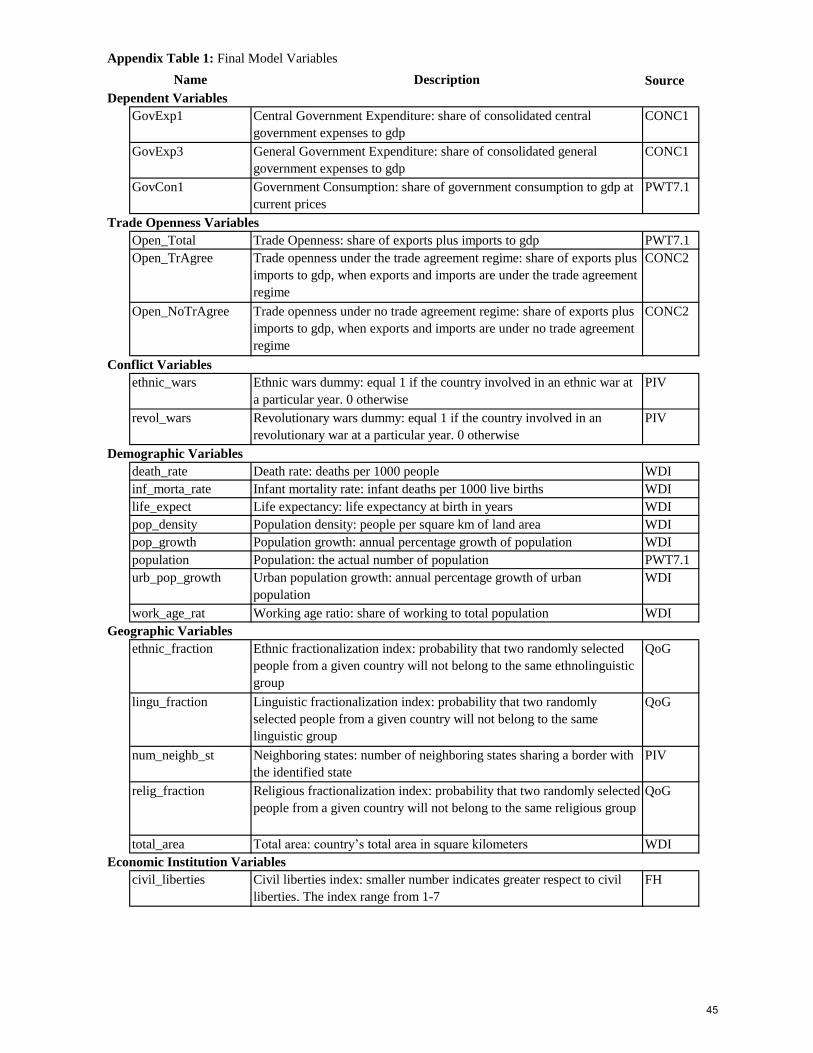
Name Description Source
Dependent Variables
GovExp1 Central Government Expenditure: share of consolidated central
government expenses to gdp
CONC1
GovExp3 General Government Expenditure: share of consolidated general
government expenses to gdp
CONC1
GovCon1 Government Consumption: share of government consumption to gdp at
current prices
PWT7.1
Trade Openness Variables
Open_Total Trade Openness: share of exports plus imports to gdp PWT7.1
Open_TrAgree Trade openness under the trade agreement regime: share of exports plus
imports to gdp, when exports and imports are under the trade agreement
regime
CONC2
Open_NoTrAgree Trade openness under no trade agreement regime: share of exports plus
imports to gdp, when exports and imports are under no trade agreement
regime
CONC2
Conflict Variables
ethnic_wars Ethnic wars dummy: equal 1 if the country involved in an ethnic war at
a particular year. 0 otherwise
PIV
revol_wars Revolutionary wars dummy: equal 1 if the country involved in an
revolutionary war at a particular year. 0 otherwise
PIV
Demographic Variables
death_rate Death rate: deaths per 1000 people WDI
inf_morta_rate Infant mortality rate: infant deaths per 1000 live births WDI
life_expect Life expectancy: life expectancy at birth in years WDI
pop_density Population density: people per square km of land area WDI
pop_growth Population growth: annual percentage growth of population WDI
population Population: the actual number of population PWT7.1
urb_pop_growth Urban population growth: annual percentage growth of urban
population
WDI
work_age_rat Working age ratio: share of working to total population WDI
Geographic Variables
ethnic_fraction Ethnic fractionalization index: probability that two randomly selected
people from a given country will not belong to the same ethnolinguistic
group
QoG
lingu_fraction Linguistic fractionalization index: probability that two randomly
selected people from a given country will not belong to the same
linguistic group
QoG
num_neighb_st Neighboring states: number of neighboring states sharing a border with
the identified state
PIV
relig_fraction Religious fractionalization index: probability that two randomly selected
people from a given country will not belong to the same religious group
QoG
total_area Total area: country’s total area in square kilometers WDI
Economic Institution Variables
civil_liberties Civil liberties index: smaller number indicates greater respect to civil
liberties. The index range from 1-7
FH
Appendix Table 1: Final Model Variables
45

Name Description Source
Political Institution Variables
chief_left Chief executive party dummy: equal 1 if the chief executive party is left.
0 otherwise
DPI
chief_military Chief Executive dummy: equal 1 if the chief executive is a military
officer. 0 otherwise
DPI
chief_nationalist Chief executive party dummy: equal 1 if the chief executive party is
nationalist. 0 otherwise
DPI
chief_regional Chief executive party dummy: equal 1 if the chief executive party is
regionalist. 0 otherwise
DPI
chief_religious Chief executive party dummy: equal 1 if the chief executive party is
religious. 0 otherwise
DPI
chief_rural Chief executive party dummy: equal 1 if the chief executive party is
rural. 0 otherwise
DPI
political_rights Political rights index: smaller number indicates greater respect to
political rights. The index range from 1-7
FH
polity_score Revised combined polity score: index showing the regime of a country.
Range from -10 (strongly autocratic regime ) to +10 (strongly
democratic regime)
PIV
Macro Policy Variables
centraliz_expense Centralization: share of central government to general government
expenses
CONC3
centraliz_tot_outl Centralization: share of central government to general government total
outlays
CONC3
gdp_per_capita Gdp per capita: in current international dollar PWT7.1
inflation Inflation: annual percentage rate of gdp deflator WDI
investment_share Investment Share: share of investment to gdp PWT7.1
Politic Variables
federal System of government: equal 1 if the system of government is federal. 0
otherwise
QoG
particip_compet Competitiveness of participation dummy: the extent to which alternative
preferences for policy and leadership can be pursued in the political
arena. Equal 1 if the preferences are competitive. 0 otherwise
PIV
political_compet Political competition index: range from 0 (repressed competition
electoral participation) to 10 (institutionalized open electoral
participation)
PIV
presidential Type of regime: equal 1 if the type of regime is presidential. 0 otherwise DPI
proportionality Electoral rule: equal 1 if the electoral rule is proportional representation.
0 otherwise
DPI
Trade Variables
political_global Political globalization index: bigger number indicates greater political
globalization. The index range from 0-100
KOF
social_global Social globalization index: bigger number indicates greater social
globalization. The index range from 0-100
KOF
DPI stand for Political Institutions database, FH stand for Freedom House database, GFS stand for Government Financial Statistics
statistic database, KOF stand for KOF Index of Globalization database, PIV stand for Polity IV database, PWT7.1 stand for Penn
World Table 7.1 database, QoG stand for Quality of Government Institute database, WDI stand for World Development Indicators
database, WTO stands for World Trade Organization database, CONC1 stand for constructed data (government expenditure data
comes from GFS and gdp data from PWT7.1), CONC2 stand for constructed data (trade agreements come from WTO and imports,
exports and gdp come from PWT7.1 - see section 3.2) and CONC2 stand for constructed data (government expenditure data comes
from GFS)
Appendix Table 1 (continued): Final Model Variables
46
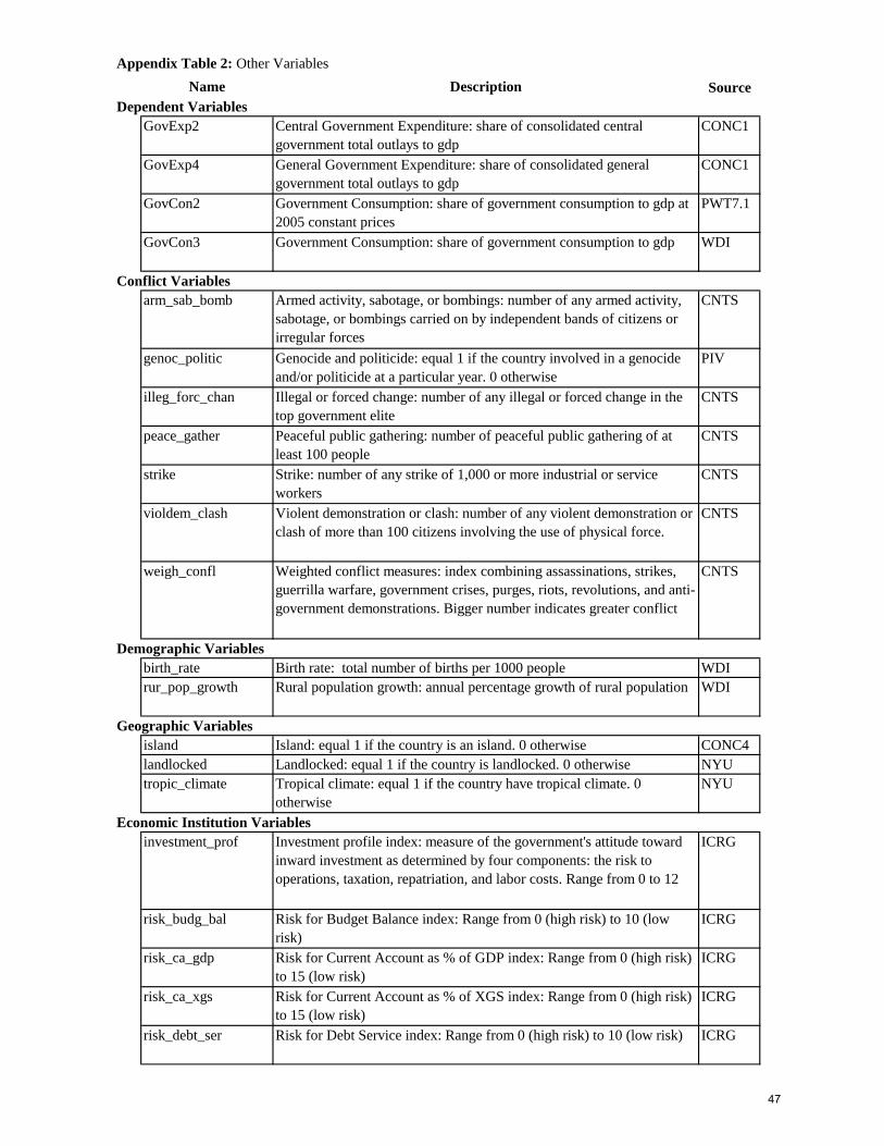
Name Description Source
Dependent Variables
GovExp2 Central Government Expenditure: share of consolidated central
government total outlays to gdp
CONC1
GovExp4 General Government Expenditure: share of consolidated general
government total outlays to gdp
CONC1
GovCon2 Government Consumption: share of government consumption to gdp at
2005 constant prices
PWT7.1
GovCon3 Government Consumption: share of government consumption to gdp WDI
Conflict Variables
arm_sab_bomb Armed activity, sabotage, or bombings: number of any armed activity,
sabotage, or bombings carried on by independent bands of citizens or
irregular forces
CNTS
genoc_politic Genocide and politicide: equal 1 if the country involved in a genocide
and/or politicide at a particular year. 0 otherwise
PIV
illeg_forc_chan Illegal or forced change: number of any illegal or forced change in the
top government elite
CNTS
peace_gather Peaceful public gathering: number of peaceful public gathering of at
least 100 people
CNTS
strike Strike: number of any strike of 1,000 or more industrial or service
workers
CNTS
violdem_clash Violent demonstration or clash: number of any violent demonstration or
clash of more than 100 citizens involving the use of physical force.
CNTS
weigh_confl Weighted conflict measures: index combining assassinations, strikes,
guerrilla warfare, government crises, purges, riots, revolutions, and anti-
government demonstrations. Bigger number indicates greater conflict
CNTS
Demographic Variables
birth_rate Birth rate: total number of births per 1000 people WDI
rur_pop_growth Rural population growth: annual percentage growth of rural population WDI
Geographic Variables
island Island: equal 1 if the country is an island. 0 otherwise CONC4
landlocked Landlocked: equal 1 if the country is landlocked. 0 otherwise NYU
tropic_climate Tropical climate: equal 1 if the country have tropical climate. 0
otherwise
NYU
Economic Institution Variables
investment_prof Investment profile index: measure of the government's attitude toward
inward investment as determined by four components: the risk to
operations, taxation, repatriation, and labor costs. Range from 0 to 12
ICRG
risk_budg_bal Risk for Budget Balance index: Range from 0 (high risk) to 10 (low
risk)
ICRG
risk_ca_gdp Risk for Current Account as % of GDP index: Range from 0 (high risk)
to 15 (low risk)
ICRG
risk_ca_xgs Risk for Current Account as % of XGS index: Range from 0 (high risk)
to 15 (low risk)
ICRG
risk_debt_ser Risk for Debt Service index: Range from 0 (high risk) to 10 (low risk) ICRG
Appendix Table 2: Other Variables
47
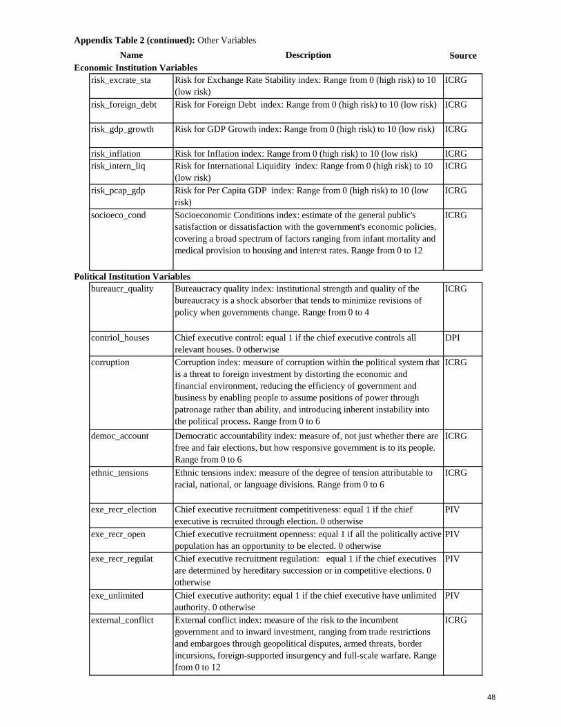
Name Description Source
Economic Institution Variables
risk_excrate_sta Risk for Exchange Rate Stability index: Range from 0 (high risk) to 10
(low risk)
ICRG
risk_foreign_debt Risk for Foreign Debt index: Range from 0 (high risk) to 10 (low risk) ICRG
risk_gdp_growth Risk for GDP Growth index: Range from 0 (high risk) to 10 (low risk) ICRG
risk_inflation Risk for Inflation index: Range from 0 (high risk) to 10 (low risk) ICRG
risk_intern_liq Risk for International Liquidity index: Range from 0 (high risk) to 10
(low risk)
ICRG
risk_pcap_gdp Risk for Per Capita GDP index: Range from 0 (high risk) to 10 (low
risk)
ICRG
socioeco_cond Socioeconomic Conditions index: estimate of the general public's
satisfaction or dissatisfaction with the government's economic policies,
covering a broad spectrum of factors ranging from infant mortality and
medical provision to housing and interest rates. Range from 0 to 12
ICRG
Political Institution Variables
bureaucr_quality Bureaucracy quality index: institutional strength and quality of the
bureaucracy is a shock absorber that tends to minimize revisions of
policy when governments change. Range from 0 to 4
ICRG
contriol_houses Chief executive control: equal 1 if the chief executive controls all
relevant houses. 0 otherwise
DPI
corruption Corruption index: measure of corruption within the political system that
is a threat to foreign investment by distorting the economic and
financial environment, reducing the efficiency of government and
business by enabling people to assume positions of power through
patronage rather than ability, and introducing inherent instability into
the political process. Range from 0 to 6
ICRG
democ_account Democratic accountability index: measure of, not just whether there are
free and fair elections, but how responsive government is to its people.
Range from 0 to 6
ICRG
ethnic_tensions Ethnic tensions index: measure of the degree of tension attributable to
racial, national, or language divisions. Range from 0 to 6
ICRG
exe_recr_election Chief executive recruitment competitiveness: equal 1 if the chief
executive is recruited through election. 0 otherwise
PIV
exe_recr_open Chief executive recruitment openness: equal 1 if all the politically active
population has an opportunity to be elected. 0 otherwise
PIV
exe_recr_regulat Chief executive recruitment regulation: equal 1 if the chief executives
are determined by hereditary succession or in competitive elections. 0
otherwise
PIV
exe_unlimited Chief executive authority: equal 1 if the chief executive have unlimited
authority. 0 otherwise
PIV
external_conflict External conflict index: measure of the risk to the incumbent
government and to inward investment, ranging from trade restrictions
and embargoes through geopolitical disputes, armed threats, border
incursions, foreign-supported insurgency and full-scale warfare. Range
from 0 to 12
ICRG
Appendix Table 2 (continued): Other Variables
48
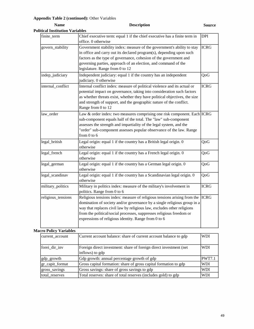
Name Description Source
Political Institution Variables
finite_term Chief executive term: equal 1 if the chief executive has a finite term in
office. 0 otherwise
DPI
govern_stability Government stability index: measure of the government's ability to stay
in office and carry out its declared program(s), depending upon such
factors as the type of governance, cohesion of the government and
governing parties, approach of an election, and command of the
legislature. Range from 0 to 12
ICRG
indep_judiciary Independent judiciary: equal 1 if the country has an independent
judiciary. 0 otherwise
QoG
internal_conflict Internal conflict index: measure of political violence and its actual or
potential impact on governance, taking into consideration such factors
as whether threats exist, whether they have political objectives, the size
and strength of support, and the geographic nature of the conflict.
Range from 0 to 12
ICRG
law_order Law & order index: two measures comprising one risk component. Each
sub-component equals half of the total. The "law" sub-component
assesses the strength and impartiality of the legal system, and the
"order" sub-component assesses popular observance of the law. Range
from 0 to 6
ICRG
legal_british Legal origin: equal 1 if the country has a British legal origin. 0
otherwise
QoG
legal_french Legal origin: equal 1 if the country has a French legal origin. 0
otherwise
QoG
legal_german Legal origin: equal 1 if the country has a German legal origin. 0
otherwise
QoG
legal_scandinav Legal origin: equal 1 if the country has a Scandinavian legal origin. 0
otherwise
QoG
military_politics Military in politics index: measure of the military's involvement in
politics. Range from 0 to 6
ICRG
religious_tensions Religious tensions index: measure of religious tensions arising from the
domination of society and/or governance by a single religious group in a
way that replaces civil law by religious law, excludes other religions
from the political/social processes, suppresses religious freedom or
expressions of religious identity. Range from 0 to 6
ICRG
Macro Policy Variables
current_account Current account balance: share of current account balance to gdp WDI
forei_dir_inv Foreign direct investment: share of foreign direct investment (net
inflows) to gdp
WDI
gdp_growth Gdp growth: annual percentage growth of gdp PWT7.1
gr_capit_format Gross capital formation: share of gross capital formation to gdp WDI
gross_savings Gross savings: share of gross savings to gdp WDI
total_reserves Total reserves: share of total reserves (includes gold) to gdp WDI
Appendix Table 2 (continued): Other Variables
49
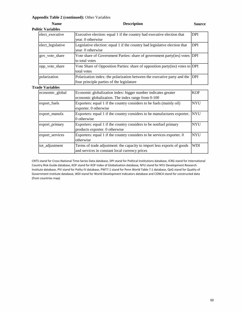
Name Description Source
Politic Variables
elect_executive Executive election: equal 1 if the country had executive election that
year. 0 otherwise
DPI
elect_legislative Legislative election: equal 1 if the country had legislative election that
year. 0 otherwise
DPI
gov_vote_share Vote share of Government Parties: share of government party(ies) votes
to total votes
DPI
opp_vote_share Vote Share of Opposition Parties: share of opposition party(ies) votes to
total votes
DPI
polarization Polarization index: the polarization between the executive party and the
four principle parties of the legislature
DPI
Trade Variables
economic_global Economic globalization index: bigger number indicates greater
economic globalization. The index range from 0-100
KOF
export_fuels Exporters: equal 1 if the country considers to be fuels (mainly oil)
exporter. 0 otherwise
NYU
export_manufa Exporters: equal 1 if the country considers to be manufactures exporter.
0 otherwise
NYU
export_primary Exporters: equal 1 if the country considers to be nonfuel primary
products exporter. 0 otherwise
NYU
export_services Exporters: equal 1 if the country considers to be services exporter. 0
otherwise
NYU
tot_adjustment Terms of trade adjustment: the capacity to import less exports of goods
and services in constant local currency prices
WDI
CNTS stand for Cross-National Time-Series Data database, DPI stand for Political Institutions database, ICRG stand for International
Country Risk Guide database, KOF stand for KOF Index of Globalization database, NYU stand for NYU Development Research
Institute database, PIV stand for Polity IV database, PWT7.1 stand for Penn World Table 7.1 database, QoG stand for Quality of
Government Institute database, WDI stand for World Development Indicators database and CONC4 stand for constructed data
(from countries map)
Appendix Table 2 (continued): Other Variables
50
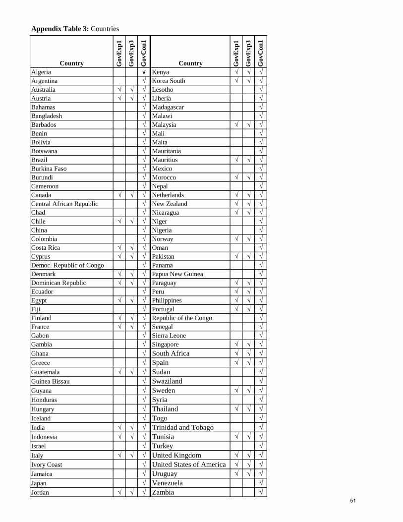
Country GovE
xp
1
GovE
xp
3
GovC
on
1
Country GovE
xp
1
GovE
xp
3
GovC
on
1
Algeria √ Kenya √ √ √
Argentina √ Korea South √ √ √
Australia √ √ √ Lesotho √
Austria √ √ √ Liberia √
Bahamas √ Madagascar √
Bangladesh √ Malawi √
Barbados √ Malaysia √ √ √
Benin √ Mali √
Bolivia √ Malta √
Botswana √ Mauritania √
Brazil √ Mauritius √ √ √
Burkina Faso √ Mexico √
Burundi √ Morocco √ √ √
Cameroon √ Nepal √
Canada √ √ √ Netherlands √ √ √
Central African Republic √ New Zealand √ √ √
Chad √ Nicaragua √ √ √
Chile √ √ √ Niger √
China √ Nigeria √
Colombia √ Norway √ √ √
Costa Rica √ √ √ Oman √
Cyprus √ √ √ Pakistan √ √ √
Democ. Republic of Congo √ Panama √
Denmark √ √ √ Papua New Guinea √
Dominican Republic √ √ √ Paraguay √ √ √
Ecuador √ Peru √ √ √
Egypt √ √ √ Philippines √ √ √
Fiji √ Portugal √ √ √
Finland √ √ √ Republic of the Congo √
France √ √ √ Senegal √
Gabon √ Sierra Leone √
Gambia √ Singapore √ √ √
Ghana √ South Africa √ √ √
Greece √ Spain √ √ √
Guatemala √ √ √ Sudan √
Guinea Bissau √ Swaziland √
Guyana √ Sweden √ √ √
Honduras √ Syria √
Hungary √ Thailand √ √ √
Iceland √ Togo √
India √ √ √ Trinidad and Tobago √
Indonesia √ √ √ Tunisia √ √ √
Israel √ Turkey √
Italy √ √ √ United Kingdom √ √ √
Ivory Coast √ United States of America √ √ √
Jamaica √ Uruguay √ √ √
Japan √ Venezuela √
Jordan √ √ √ Zambia √
Appendix Table 3: Countries
51

Variable GovE
xp
1
GovE
xp
3
GovC
on
1
Way of Entering into the Model
GovExp1 √ ln(5-Year Average)
GovExp2 ln(5-Year Average)
GovExp3 √ ln(5-Year Average)
GovExp4 ln(5-Year Average)
GovCon1 √ ln(5-Year Average)
GovCon2 ln(5-Year Average)
GovCon3 ln(5-Year Average)
Open_NoTrAgree √ √ √ ln(5-Year Average) - ln(1+X)
Open_Total √ √ √ ln(5-Year Average) - ln(1+X)
Open_TrAgree √ √ √ ln(5-Year Average) - ln(1+X)
centraliz_expense √ √ ln(5-Year Average)
centraliz_tot_outl ln(5-Year Average)
chief_left √ √ 5-Year Average
chief_military √ √ 5-Year Average
chief_nationalist √ √ 5-Year Average
chief_regional √ √ 5-Year Average
chief_religious √ √ 5-Year Average
chief_rural √ √ 5-Year Average
civil_liberties √ √ √ ln(5-Year Average)
death_rate √ √ √ ln(5-Year Average)
east_asia&pacific √ √ √ 5-Year Average
ethnic_fraction √ √ √ ln(5-Year Average)
ethnic_wars √ √ √ 5-Year Average
federal √ √ √ 5-Year Average
gdp_per_capita √ √ √ ln(Initial Value)
inf_morta_rate √ √ √ ln(5-Year Average)
inflation √ √ √ 5-Year Average
investment_share √ √ √ ln(5-Year Average)
latin_amer&carib √ √ √ 5-Year Average
life_expect √ √ √ ln(5-Year Average)
lingu_fraction √ √ √ ln(5-Year Average)
mid_east&nor_afr √ √ √ 5-Year Average
north_america √ √ √ 5-Year Average
num_neighb_st √ √ 5-Year Average
particip_compet √ √ 5-Year Average
political_compet √ √ ln(5-Year Average)
political_global √ √ √ ln(5-Year Average)
political_rights √ √ √ ln(5-Year Average)
polity_score √ √ 5-Year Average
pop_density √ √ √ ln(5-Year Average)
pop_growth √ √ √ 5-Year Average
population √ √ √ ln(5-Year Average)
presidential √ √ √ 5-Year Average
proportionality √ √ 5-Year Average
relig_fraction √ √ √ ln(5-Year Average)
revol_wars √ √ √ 5-Year Average
social_global √ √ √ ln(5-Year Average)
south_asia √ √ √ 5-Year Average
subsaharan_africa √ √ √ 5-Year Average
total_area √ √ √ ln(5-Year Average)
urb_pop_growth √ √ √ 5-Year Average
work_age_rat √ √ √ ln(5-Year Average)
Appendix Table 4: Variables
52


![Openness Agreements: Part Two The Reality of Openness · Presented by © Adoptive Families Association of BC [2016] Openness Agreements: Part Two The Reality of Openness](https://img.pdfslide.us/doc/110x75/5e81797d22c1fb32191241b3/openness-agreements-part-two-the-reality-of-openness-presented-by-adoptive-families.jpg)