Embed Size (px)
Citation preview


Are Business Cycles All Alike? A BandpassFilter Analysis of the Italian and US Cycles∗
Mauro Napoletano† Andrea Roventini◦ Sandro Sapio‡
October 20, 2005
Abstract
In this paper, we perform an empirical comparison of Italian and U.S.business cycles. After filtering the time series of the main macroeco-nomic variables of the two countries, through an approximate band-pass filter, we analyze the cross-correlations between each filtered vari-able and the filtered GDP, indicator of the business cycle.
We find heterogeneity in business cycle dynamics as regards vari-ables related to the industrial structure (see exports, investment inconstruction), and to the organization of markets (e.g. stock prices,private consumption), interpreted as effects of local path-dependencies.Cyclical components of prices, labor market variables, and monetarypolicy indicators are almost invariant across economies, reflecting com-mon international drivers, such as the Federal Reserve Bank monetarypolicy, and international oil prices.
Keywords: Business Cycles, Bandpass Filter, Cross Correlations,Italian Economy, Macroeconomics.
JEL Classification: C22, E32.
∗We are grateful to Marco Lippi, Carlo Bianchi, to an anonimous referee, and to con-ference participants in Bologna (Annual Meeting of the Italian Economic Association,October 2004) and in Venice (First Italian Congress of Econometrics and Empirical Eco-nomics, January 2005) for helpful comments and suggestions. All usual disclaimers apply.
†S. Anna School of Advanced Studies, Pisa, and Polytechnic University of Marche,Ancona. E-mail: [email protected].◦ S. Anna School of Advanced Studies, Pisa and University of Modena and Reggio Emilia.E-mail: [email protected].‡S. Anna School of Advanced Studies, Pisa.E-mail: [email protected]
1

1 Introduction
In this paper, an international comparison between the statistical propertiesof Italian and U.S. business cycles is proposed. After filtering the time seriesof the most relevant macroeconomic variables of the two countries, throughan approximate bandpass filter, we study the cross-correlations between eachfiltered variable and the filtered real GDP, used as benchmark indicator ofthe business cycle.
The aim of the analysis is to answer to a simple question: “Are businesscycles all alike across countries?”. We are interested in detecting invariancesand diversities in the behavior of the main macroeconomic variables at busi-ness cycle frequencies, and in deducing the economic mechanisms - in termsof common and idiosyncratic drivers - behind the observed patterns.
Business cycles are among the most salient features of the aggregate dy-namics of industrialized economies. As such, they have been the topic of alarge number of theoretical and empirical studies, which typically see macro-economic dynamics as driven by stochastic trends, resulting from the accu-mulation of random shocks, with varying degrees of persistence and differentperiodicities. Business cycle dynamics is mapped into a specific set of short-to-medium run frequencies, and the analysis is usually focused on variablesresulting from the application of filters meant to isolate the business cyclecomponent. Many procedures have been deviced, such as linear trend re-moval, first differencing, the Hodrick-Prescott (1981) filter, wavelets, andthe bandpass filter (Baxter and King, 1999).
The latter, characterized by particularly appealing properties, has beenfirst applied by Stock and Watson (1999) on U.S. data. More recently, inter-national comparisons have been performed, e.g. Agresti and Mojon (2001),who focus on E.U. countries. Interestingly, Agresti and Mojon tend to under-line the similarities between business cycles in European countries, as well aswith the U.S., much more than their differences, so much as to conclude thatmodels conceived originally for the U.S. economy can provide good approxi-mations for E.U. countries, too. On the other hand, even a quick comparisonbetween the Stock-Watson results and works focused on the Italian economy,such as Gallegati and Stanca (1998), shows that cross-country differences arefar from negligible.
The present study takes part into the debate, and adds evidence thatcountry-specific features are key in determining which variables prompt andwhich respond to business cycles. Heterogeneity in business cycle dynamicsis detected as regards private consumption, government expenditure, invest-ments, exports, credit, and share prices. On the contrary, business cyclecomponents of prices, wages, employment, unemployment, labor productiv-
2

ity, interest rates, and money aggregates display almost invariant propertiesacross the analyzed economies.
We interpret differences in business cycle properties as effects of localpath-dependencies, and invariances as reflecting the impact of common in-ternational drivers. Moreover, we put forward some conjectures as to thesources of common and idiosyncratic components. Specifically, internationalcoordination mechanisms such U.S. monetary policy and oil prices may havedriven the similar dynamics in money, prices and labor markets in Italy andin the U.S., whereas differences in business cycles may be related to path-dependencies in the industrial structure (see exports, investment in construc-tion), and in the organization and development of markets (cf. stock prices,private consumption).1
The paper is organized as follows. In Section 2, we describe the bandpassfilter and the cross-correlation analysis, and we explain the criteria utilized forour classification of comovements. Section 3 describes the available datasetand gives an account of the results. Conclusions and perspectives are inSection 4.
2 Methodology
The first quantitative enquiry on business cycle dynamics can be found inthe work of Burns and Mitchell (1946), which was based on a careful analysisof a wide set of macroeconomic variables, during the various business cyclestages. It aimed at classifying variables into leading, coincident and lagging,depending on the number of months it takes to reach peaks and troughs ofthe business cycle. Such a qualitative method is nowadays known as theNBER approach.
As defined by Burns and Mitchell,
a (business) cycle consists of expansions occurring at aboutthe same time in many economic activities, followed by similargeneral recessions, contractions and revivals which merge intothe expansion phase of the next cycle; this sequence of changesis recurrent but not periodic; in duration business cycles varyfrom more than one year to ten or twelve years; they are notdivisible into shorter cycles of similar character with amplitudesapproximating their own.
1See Arthur (1994), David (1985), and Castaldi and Dosi (2005), for the concept ofpath-dependence.
3

Consistent with the above, the empirical analysis of business cycles re-quires (i) retrieving the business cycle component of each macroeconomictime series, and (ii) estimating comovements between business cycle com-ponents of various macroeconomic variables. The former step is the mostcontroversial of the two, as it requires an operational definition of businesscycle.
The very idea that macroeconomic variables include a business cycle com-ponent is rooted in a widely used methodological tool, the so-called tradi-tional decomposition, or model with unobserved components, according towhich a macroeconomic variable (in logs) can be expressed as the sum oftrend (T), cycle (C), seasonal (S), and irregular (I) components, as follows:
Y = T + S + C + I
The trend includes long-term fluctuations of any nature, deterministic(such as linear and quadratic trends), as well as stochastic (e.g. I(1) and I(2)components). The seasonal refers to systematic fluctuations with periodicityshorter than one year. The irregular conveys high-frequency random shocks.Macroeconomics typically focuses on the business cycle component, whichis about non-periodic cycles at short-to-medium run frequencies. Harvey(1985), Watson (1986), Clark (1987), and Harvey and Jaeger (1993) areamong the main contributors to this methodological stream.
It is worth noting that such a decomposition is crucially based on twoassumptions: (a) there exists a log-linear relationship between the observedvariable and its unobserved components; (b) components are mutually inde-pendent. These are perhaps too restrictive conditions.2One would rather liketo avoid imposing any specific model on the data.
Therefore, the approach followed here is somewhat different. FollowingMurray (2003), our working definition of business cycle is what remains ofa series, after frequencies outside a given frequency band are filtered out.Notice that the choice of the relevant frequency band was already suggestedby Burns and Mitchell’s definition. In terms of assumptions, the definitionused here is less demanding than the unobserved component model. Spectralmethods based on the Fourier Transform seem proper vis-a-vis the implemen-tation of this definition.3
2See, for instance, Zarnowitz (1997) for critical remarks on the independence betweencycles and long-run growth.
3A criticism to the Fourier-based approach to spectral analysis as regards empiricalmacroeconomics is grounded on wavelet analysis. See Ramsey (1999) for a review ofwavelets for economists. A recent application to macroeconomic time series is providedby Gallegati, Gallegati, Ramsey, and Semmler (2004).
4

In this respect, our methodology is line with the early work by Engle(1974), and with more recent analyses by Stock and Watson (1999), Gallegatiand Stanca (1998), Agresti and Mojon (2001), and Christiano and Fitzgerald(2003). Hodrick and Prescott’s (1981) work and follow-ups can be seen asmembers of this family, too.
2.1 Estimating the business cycle component
Estimation of the business cycle, as defined above, is usually accomplished bytransforming the observed series, through application of a filter. The choiceof the proper filter is crucial, in that, as pointed out by Canova (1998; 1999),different methods may affect both the qualitative and quantitative stylizedfacts of the business cycle.
According to Baxter and King (1999), the ideal filter for business cycleanalysis should meet the following properties. First, trend-reduction, i.e., theproperty of removing long-run trends.4 Second, high frequency components(i.e. seasonal and irregular) ought to be smoothed out, too. Third, nophase shifts should be induced, meaning that timing relationships betweenvariables should not be altered. This is a key requirement, in that isolatingbusiness cycle components is only an intermediate step towards studyingcomovements. Fourth, one would like the filtering outcome to be independentof the length of the original series. In other words, if the sample is updatedas new observations are made available, further application of the filter mustyield a series with the first n values equal to the business cycle componentpreviously estimated over a sample size of n. Fifth, it is desirable that thefiltered series are able to track the NBER dating of business cycles, which istaken as a benchmark.
Baxter and King (1999) showed that a symmetric and stationary band-pass filter satisfies all the above requirements, while outperforming previousapproaches, such as linear trend removal, first differencing, and the Hodrick-Prescott filter. 5
The starting point is the Cramer representation of a time series, accordingto which a sequence {yt} can be approximated by an integral sum of mutually
4As first shown by Granger (1964), the “typical spectral shape” of a macroeconomicvariable is monotonically decreasing, meaning that the bulk of the variance is attributableto very low frequency components (such as long-run trends) and, albeit to a lesser extent, tobusiness cycle (or medium frequency) fluctuations. The strong contribution of frequenciesaround zero is the reason why business cycle analysis requires a prior detrending of theoriginal series.
5See also Zarnowitz and Ozyildirim (2002) for an extensive discussion on this point.
5

orthogonal random periodic components, with frequencies ω ∈ [−π, π]:
yt =∫ π
−πeiωtξ(ω)dω (1)
Based on the above equation, the variance of yt can be decomposed asfollows:
var(yt) =∫ π
−πfy(ω)dω (2)
where fy(ω) = var(ξ(ω)) is defined as the power spectrum of yt. Thelatter provides information about the contribution of any periodic componentto the total variance of yt.
Suppose now we filter yt as follows, to yield the new series y∗t :
y∗t = a(L)yt (3)
where
a(L) =∑+∞
h=−∞ ahLh
is a two-sided moving average filter, with infinite leads and lags, expressedas a polynomial in the lag operator L (such that Lhyt = yt−h). The associatedspectral representation reads:
y∗t =∫ π
−πeiωtα(ω)ξ(ω)dω (4)
where α(ω) =∑+∞
h=−∞ aheiωh is the so-called frequency response function,
mapping each frequency ω into the extent to which the filter alters the weightof the periodic component ξ(ω) in the spectral decomposition. Accordingly,the variance of y∗t is decomposed as follows:
var(y∗t ) =∫ π
−π|α(ω)|2fy(ω)dω (5)
where |α(ω)|2 denotes the spectral transfer function, a measure of theeffect of the filter on the variance contribution at frequency ω.
The above equations allow to define the outcome of any filtering procedureand, in turn, the filter required for that outcome to be achieved. One maywant to isolate frequencies belonging to some interval [ω′, ω′′], |ω′| ≤ |ω′′|. Insuch a case, the ideal filter must satisfy α(ω) = 1 if ω′ ≤ |ω| ≤ ω′′, α(ω) = 0otherwise.
In order to meet the trend reduction property, the condition α(0) = 0should hold, so that the filtered series does not display any power at zerofrequency. This in turn requires α(0) =
∑+∞h=−∞ ahe
i0h =∑+∞
h=−∞ ah = 0,
6

i.e. the application of a symmetric moving average filter in the time domain,with weights summing up to zero.6
In practice, the ideal bandpass filter cannot be used: it has to be replacedby an approximate bandpass filter, entailing finite leads and lags, say K. Fora given K, the associated frequency response function, denoted as αK(ω), ischosen by minimizing a loss function such as
Q =∫ π
−π|α(ω)− αK(ω)|2dω (6)
In the above criterion, the goodness of the approximation is measured bythe integral sum of squared deviations between the approximate and idealfilters.7 Because the outcome of the above minimization problem is sensitiveto K, this ought to be carefully chosen. Of course, as K grows large, one canachieve better approximations, but because 2K observations are lost, there isa cost in terms of sample size. Moreover, cutting off the moving average filtergives rise to two distortionary effects: leakage (i.e. overstating frequenciesoutside of the band of interest) and compression (i.e. underrepresenting thefrequencies one wants to focus on). The choice of K must account also forthis. The solution to these trade-offs is mainly an empirical matter.8
Summing up, the application of a bandpass filter requires setting threeparameters: two defining the breadth of the frequency band of interest (lowerbound ω′ and upper bound ω′′); and a cut-off parameter (K). Conditionalon these choices, the bandpass filter yields a stationary series, with variance(almost) completely attributable to frequencies between ω′ and ω′′.
2.2 Estimating Comovements
Once estimates of business cycle components of many macroeconomic vari-ables have been obtained, one can measure their mutual correlations. Acommon way to do this is to define a benchmark variable, which is thoughtto represent the business cycle, and to estimate cross-correlations of all othervariables with respect to this one, at various leads and lags. This is for ex-ample the approach applied by Stock and Watson (1999) to U.S. quarterlydata, and by Agresti and Mojon (2001) to quarterly data for E.U. countries.
6Another possibility is to apply the filter directly in the frequency domain, but estimatesof the spectrum are not unaffected by the length of the series. As an implication, one ofthe requirements mentioned above cannot be met. See Canova (1998) for an example, andBaxter and King (1999) for a caveat.
7A generalization of this loss function, entaling weighted integral sums of squared de-viations, is provided by Christiano and Fitzgerald (2003).
8Baxter and King recommend to set K = 12, because higher values do not lead tosignificant improvements in the performance of the filter.
7

The aim is to build a taxonomy of macroeconomic variables according tofive dimensions: (i) sign, (ii) magnitude, and (iii) timing (in leads and lags)of the cross-correlations with respect to “the cycle” (i.e. to the benchmarkvariable representing it); as well as (iv) amplitudes of the fluctuations, and(v) predictive ability.
As commonly done, here we use the filtered GDP as benchmark vari-able.9 It may be pointed out that a composite index may provide a betterapproximation of the business cycle. However, previous work by Gallegatiand Stanca (1998), who performed a sensitivity analysis on the benchmarkvariable, shows that results are robust to the benchmark chosen. We computecross-correlations between each variable at time t, and the GDP at all leadsand lags from t− 6 to t + 6. Then, we look at the sign and the magnitude ofcross-correlations, and we investigate on the existence of patterns.
A variable is said to be “procyclical” if its cross-correlogram displayspositive values around lag zero and resembles the shape of the GDP auto-correlogram; “countercyclical” if the cross-correlogram pattern - in terms ofsign and shape - is inverse to the one displayed by the GDP autocorrelogram;and “acyclical” if its cross-correlogram does not exhibit any definite patternwith respect to the GDP autocorrelogram.
As it will be noted, some variables display cross-correlograms which aresimilar to the GDP autocorrelogram, but slightly “out-of-phase”: i.e., reach-ing their maximum (or minimum if countercyclical) at some different leads orlags. If the absolute maximum (or minimum) is achieved at some GDP lead,then the variable is denoted as “leading”, whereas it is called “lagging” inthe opposite case. This definition in turn implies that the cross-correlationsof leading (lagging) variables tend to decay more slowly than GDP autocor-relations when considering future (past) GDP. Finally, “coincident” variablesare those displaying the bulk of their cross-correlation with GDP at lag zero.
Amplitudes of fluctuations can be measured in terms of relative variances,computed with respect to the variance of the filtered GDP. These are usefulto distinguish between variables according to whether they are more or lessvolatile than the cycle.
Finally, further information as to the predictive ability of macroeconomicvariables may complement the above set of dimensions. This is obtainedthrough simple, bivariate Granger-causality tests, performed using the GDPand any given variable.10
9Henceforth, the term “GDP” shall denote the filtered GDP.10Granger causality does not correspond to the causality concept usually referred to in
the economic discourse. A variable might well predict GDP growth not because it is afundamental determinant of GDP growth but just because it embeds information on somethird variable which is itself a determinant of GDP growth. In addition, the predictive
8

3 Empirical Analysis and Results
Our analysis is performed on seasonally-adjusted quarterly data from theOECD Main Economic Indicator and Quarterly Labour Force Statistics databases. We apply the bandpass filter to the natural logarithm of all thevariables that are not expressed in percentage points. Lists of variables areprovided in Tables 1 and 2. For most series, the sample period goes fromthe 1st quarter of 1970 to the 3rd quarter of 2002.11 In order to define theduration of the Italian business cycle, we follow Stock and Watson’s (1999)approach, i.e. we set the lower and upper bounds as the shortest and longestfluctuations experienced by the Italian economy in the period under analysis.Consistent with the chronologies of the Italian business cycles reported byGallegati and Stanca (1998), frequencies ranging from 9 to 43 quarters areconsidered. Hence, our upper and lower bounds for Italian series are differentfrom the ones set by Stock and Watson for the U.S. series (6 and 32 quarters).This is justified by the evidence that, in the last 30 years, Italian businesscycles have been longer than the American one (see Agresti and Mojon,2001, more generally on European economies). In line with Baxter and King(1999) and Stock and Watson (1999), we set the cut-off parameter K to 12.However, given that some of our series start as late as 1980, we decided tobarter a lower precision with a higher number of usable observations. Hence,following Agresti and Mojon (2001), the filtering is performed using K = 8as well.
3.1 Basic Statistical Properties
Basic properties of the filtered series are shown in Table 3. These tableprovides information about mean, variance, skewness and kurtosis of eachbandpass filtered variables, for K = 12. Using a different cut-off parameter(K = 8) does not yield significant deviations from the statistics reported inthe table12.
First, let us have a look at variances. In this respect, Italy and U.S. showsimilar patterns: the most volatile variables are share prices, unemployment,
content of each relation tested in Tables 6 and 7 can be altered by the inclusion ofadditional variables. Nevertheless, those tests give a quantitative measure of forecastingability in bivariate relations which theoretical models must be consistent with.
11The most important exceptions are the money and credit series, whose sample periodgoes from the 1st quarter of 1975 to the 4th quarter of 1998, when the EMU becameoperative.
12Fixing K = 8 does not significantly alter the cross-correlation structure either. Hence,in the next section, we only report the cross-correlations for K = 12.
9
foreign trade indicators, and investment variables.13
Second, by analyzing kurtosis values we notice that there exists a set ofvariables with negative excess kurtosis (i.e. more platykurtic than a Normallaw). This set, which is shared by the two countries, includes total credit toprivate sector, the official discount rate, and share prices.
Furthermore, the cyclical components of labor market variables and ofmoney aggregates in Italy are more exposed to extreme events than in theU.S. For instance, the excess kurtosis for the growth rate of wages is 1.35in Italy, as compared to 0.02 in the U.S., and 1.86 for the Italian inflationrate, vis-a-vis 0.66 in the U.S.. We also find the excess kurtosis of Italianemployment to be 1.37, much higher than for the U.S. (0.04). Similar resultshold for the money aggregates (M1 and M2). The opposite occurs for importsand labor productivity: the distribution of these filtered variables displayslarger departures from normality in the U.S. than in Italy.
Finally, U.S. variables within the monetary and foreign trade sectors tendto be less similar to each other, than in Italy. More specifically, the bandpassfiltered M1 in the U.S. is almost three times more volatile than M2, while inItaly M1 and M2 display basically the same variance. Furtherly, imports andexports in the U.S. are different in terms of skewness (negative for imports,very close to zero for exports) and as regards excess kurtosis (positive onlyfor imports).
3.2 Cross-correlation Analysis
The results of the cross-correlation analysis for our Italian and U.S. dataare summarized in Tables 4 and 5. Each entry is the correlation of eachbandpass-filtered variable at time t, with the bandpass-filtered GDP, takenas the benchmark indicator of the business cycle, at all leads and lags withina range of 6 quarters.
A detailed description of results is provided as follows. We proceed forhomogeneous groups of variables. The identification of the cyclical natureof the variables analyzed is based on the criteria explained in Section 2.2.Comparisons between our results for the two countries, as well as with theresults of previous analyses - specifically, Stock and Watson’s (1999) studyon U.S. data - are meant to shed light on invariances and specificities ofthe Italian and U.S. business cycles, and on the robustness of the patternsdetected.
GDP Components. Bandpass-filtered variables considered here are:
13We can only compare the standard deviations of series that have the same units (e.g.natural logarithm).
10

private final consumption, government final consumption, gross fixed capitalformation (GFCF), exports, and imports. See Figures 1 and 7.
Private final consumption is positively correlated with the GDP over thecycle; in Italy, it is a coincident indicator, whereas it leads the GDP in theU.S. Furthermore, it Granger-causes GDP in Italy (see Table 6), whereas inthe U.S., the causality runs in both directions (see Table 7).
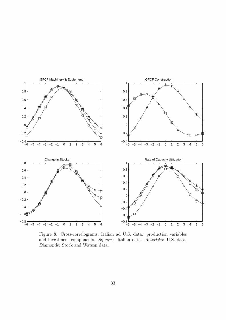
The bandpass filtered GCFC is procyclical in both countries. It is aslightly lagging variable in Italy, whereas in the U.S. it is synchronized withthe cycle. Differences among the two countries emerge also with respectto Granger-causality relationships between aggregate investment and GDP.Indeed, GCFC does not have any causal relationship with GDP in Italy,whereas it appears to be predicted by the latter variable in the U.S. Inter-estingly, the analysis of more disaggregated investment series reveals someheterogeneity between the cyclical behaviors of investment in construction(lagging in Italy, coincident in the U.S.). Fig. 2 and lower charts of Fig. 8illustrate these patterns.
Government final consumption exhibits a coincident and countercyclicalbehavior in Italy, and a lagging and procyclical pattern in the U.S. However,in both countries, most of the cross-correlations are not significantly differentfrom zero. A possible explanation for this result is that government finalconsumption includes expenses that tend to vary little with business cycles(e.g. labor retirement payments, health care outlays), as well as the so-calledautomatic stabilizers.
Both imports and exports display a procyclical pattern. However, whileimports tend to be coincident in both countries, exports display oppositebehaviors (leading in Italy vs. lagging in the U.S.). Consequently, the tradebalance is leading in Italy, lagging in the U.S. These patterns are not rejectedby the Granger causality analysis (cf. Tables 6 and 7). In Italy, exportsdisplay both causal relations with respect to GDP in a simple bivariate model,whereas they appear to be predicted by GDP in the U.S. Finally, imports donot have any causal relation with GDP in both countries considered.
Production Process. Industrial production, change in stocks, and therate of capacity utilization are under focus here (see Fig. 3 and the uppercharts of Fig. 8). All three are procyclical and coincident indicators. Forthis group of variables, cross-correlations do not reveal any remarkable dif-ferences between Italy and the U.S. More interesting is the bivariate causalrelationship between the rate of capacity utilization and the GDP. In theU.S., the former variable helps forecasting the latter, whereas the relation-ship is inverted in Italy.
Labor Market. Italian total employment and total unemployment are
11

significantly correlated with lagged GDP (cf. Figures 4 and 9).14 Totalemployment is procyclical, whereas total unemployment is countercyclical.These correlation patterns are in accordance with those found for the U.S.However, magnitudes are generally higher for U.S. variables. Moreover, thetransmission of a GDP shock to the unemployment level requires much moretime in Italy than in the U.S.
As implied by the Okun’s law, labor productivity, measured as the ratiobetween GDP and total employment, is expected to be procyclical. Thisindeed occurs: Figures 4 and 9 display a clearly procyclical and slightlyleading pattern for both Italy and the U.S. This is consistent with the evi-dence of a procyclical total employment.
Prices and Wages. Indicators of prices and wages (Figures 5 and10) are supposedly characterized by very similar statistical properties. Thecomparison across countries, however, might reveal interesting information.Cross-correlations with the GDP show that CPI and hourly wage ratesare leading and countercyclical variables in both Italy and the U.S. Cross-correlations with lagged GDP are stronger for the CPI than for the wage rate(roughly -0.70 vs. -0.55). Remarkably, magnitudes are very similar acrosscountries.
Relevant differences emerge as the bandpass filtered rates of change comeunder focus. Indeed, in Italy the CPI inflation and the growth rate of wagesare coincident and procyclical, while in the U.S. they tend to lead the cycle,and to be negatively correlated with it.
Notice, however, that the picture is less clear than with respect to levelvariables. For instance, the U.S. wage growth displays strong cross-correlations(around 0.30) with past GDP. Something similar occurs for other growth ratevariables, also in Italy: the relationship of growth rates with the GDP acrossthe cycle is somewhat blurred.
In both countries analyzed bivariate tests do not help discerning clearcausality relationships among labor-market variables and GDP or amongprice variables and GDP. In most cases (cf. Tables 6 and 7) the hypothesisof Granger causality is accepted or rejected in both directions.
Money and Finance. Turning the attention to monetary and finan-cial variables (Figures 6 and 11), we observe that both monetary aggregatesanalyzed (M1 and M2) exhibit a procyclical and leading pattern in bothcountries. Furthermore, money appears to Granger-cause output in bothcountries, as long as larger money aggregates are considered (see Tables 6and 7).
14We have also analyzed the rate of unemployment. However, its pattern is not verydifferent with respect to the one displayed by the unemployment level.
12

Total domestic credit displays heterogeneity across countries. Credit leadsthe cycle in Italy, and it is negatively correlated with it. On the contrary,U.S. commercial bank loans tend to lag the cycle, and to have positive cross-correlations. This divergence may stem from the imperfect comparability ofthe two variables as well as from the different institutional setups character-izing the financial system of the two countries. Nonetheless, it does not seemto affect the ability of credit to predict cyclical movements of GDP. Indeed,all credit variables considered Granger-cause GDP both in Italy and in theU.S.
On the grounds of our results, a countercyclical and leading relationshipcan be detected between bond yields and the GDP over the business cycle.Indeed, the cross-correlation with lagged GDP is negative in both countries,between -0.50 and -0.60. Similar results seem to hold for official discountrates, although positive cross-correlations with past GDP are pretty strong.The Granger causality tests in Table 7 provide additional evidence on thelinks between interest rates and output movements in the U.S.: both shortand long term interest rates display predictive ability with respect to GDPin the U.S.15 As far as Italy is concerned, official discount rates appear to bepredicted by GDP, whereas no causal relation emerges between bond yieldsand GDP.
Overall, the foregoing findings support the idea that, in the analyzedperiod, monetary policy has been effective, although with some lag.16
The results on share prices indicate a lagging procyclical pattern in Italy.The cross-correlations with GDP from time t onwards are not significantlydifferent from zero, suggesting the absence of any forecasting property of theItalian stock prices during the period analyzed. The bivariate Granger testsin Table 6 confirm the foregoing conjecture. A different result holds for theU.S., where stock prices are moderately procyclical and tend to lead the cycle.Nonetheless, also in the U.S. they lack any bivariate causal relationship withGDP.
3.3 Summary and Discussion of Results
In discussing results, we shall go through the main similarities and differencesbetween business cycle comovements in Italy and in the U.S.
First, both countries share very similar comovement patterns as regardsemployment, price and wage levels, labor productivity, as well as money ag-gregates and interest rates. In other words, comovements of price levels and
15In the U.S. long term interest rates are also Granger-caused by GDP.16We preferred not to analyze measures of the real interest rate. We were dissuaded by
the big uncertainty surrounding the construction of any measure of that variable.
13

quantities in the labor and monetary markets are similar across countries. Inboth, CPI, wages and interest rates are leading and countercyclical indicatorsof the business cycle. Money, and labor productivity are leading too, but pro-cyclical. Labor market series are lagging; unemployment is countercyclical,whereas employment is procyclical.
Relevant differences are instead detected as to consumption, governmentexpenditure, investments, exports, credit, and share prices. More in detail,U.S. expansions seem to be anticipated by increases in consumption, gov-ernment expenditure, and stock prices, and followed by wider availability ofcommercial bank loans, by greater investment in machinery and equipment,and by surges in import.
This does not occur in Italy, where decreases in credit and increases in im-ports and in the rate of capacity utilization typically signal that the economyis going to expand, while positive changes in stock prices and in constructioninvestments tend to show up with some lag.
Finally, in both countries CPI and wage inflation rates are character-ized by peculiar cross-correlation patterns. Indeed, according to Zarnowitz(1997), growth rates naturally tend to decrease in absolute value at the endof each stage of a business cycle (expansions as well as contractions), i.e., justbefore reaching a peak or a trough. On the contrary, their absolute valueincreases quite rapidly at the inset of a new stage. As an implication, theydisplay positive contemporaneous correlation with the last part of a contrac-tion, and with the inset of an expansion, but a negative one with the lastpart of an expansion and with the inset of a contraction. By definition, aprocyclical (countercyclical) variable is characterized by positive (negative)contemporaneous correlation with the cycle, regardless of the stage. Hence,our procyclicality and countercyclicality concepts might not fit the analysisof growth rates.
4 Conclusions
In this paper, we have compared the statistical properties of Italian and U.S.business cycles. After filtering the time series of the most relevant macro-economic variables of the two countries, through an approximate bandpassfilter, we have analyzed the cross-correlations between each filtered variableand the filtered real GDP, used as benchmark indicator of the business cycle.
Interestingly, it appears that which variables prompt and which respondto business cycles depends on country-specific features, despite the similarlevel of development of the two countries. Heterogeneity in business cycledynamics is detected as regards variables related to the industrial structure
14

(see imports, investment in construction), and to the level of organizationand development of markets (cf. stock prices, private consumption). Onthe contrary, business cycle dynamics of labor market and monetary policyvariables is basically invariant across the analyzed economies, despite somewell-known differences (e.g. in unemployment rates).
The distinction between country-specific and invariant properties is basedon some fundamental questions: Can one identify common drivers of inter-national business cycles? And which mechanisms lay behind common trendsand idiosyncratic factors?
Macroeconomic variables in two countries can behave in a similar wayjust as a result of random forces, or because their dynamics are driven bycommon trends. Cross-country heterogeneities in business cycle behaviors,instead, signal that local driving mechanisms are most important.
If we can identify international coordination mechanisms which tie eco-nomic fluctuations of different countries together, then we expect invariancesto show up only as regards the economic sectors which are directly involved.Among the possible examples: (i) the existence of a leader-follower rela-tionship as to monetary policies (the Italian central bank as a follower ofthe U.S. Federal Reserve policy moves); (ii) the exposure to common priceshocks, such as those affecting oil prices (oil being a pervasive input in botheconomies, and its price being set by a cartel such as the OPEC).
The variables most likely affected are interest rates, money aggregates,prices, wages, employment, and unemployment. Notice that cross-countrysimilarity in cyclical properties of labor market variables in not a trivial re-sult: these markets are organized in quite different ways in Italy and in theU.S. One may thus expect their dynamics to differ quite substantially. Find-ing common cross-country properties means that the effect of idiosyncraticfactors is more than offset by the effect of common drivers. In other words,institutional differences in labor market organizations do not show up in dataso much as the impact of international trends.
Whenever we find significant differences in cyclical dynamics, we can in-terpret them as the effect of relevant idiosyncratic factors, outcomes of path-dependent growth processes. Different initial conditions can lead to dramaticdiversities in dynamics. First, substantially different sectoral structures canemerge, implying, for instance, different patterns of imports and exports. Asecond possible outcome is diversity in the way financial and credit marketsare organized, and relatedly in their actual impact in the economy. For in-stance, the credit market design can strongly affect the ability of consumersto borrow money, and thus determine more or less strict constraints on, say,their intertemporal allocation of income between consumption and saving.
As a conclusion, our results imply that business cycle dynamics can be de-
15

scribed in terms of (i) path-dependent processes and (ii) coordination mech-anisms. Partially quoting Burns and Mitchell, we can see a national businesscycle as a sequence of expansions, recessions, contractions and revivals oc-curring at about the same time in many economic activities; such a sequencepreserves its properties across countries, to the extent that international co-ordination mechanisms more than offset the effect of idiosyncratic factorsengendered by local path-dependent processes. Broader comparative studiesare needed in order to assess the robustness of our conclusions.
References
[1] Agresti A., and B. Mojon, 2001, “Some Stylised Facts on the Euro AreaBusiness Cycle”, European Central Bank, working paper 95.
[2] Arthur B., 1994, Increasing Returns and Path-Dependence in the Econ-omy. Ann Arbor, Mich, University of Michigan Press.
[3] Baxter M., and R.G. King, 1999, “Measuring Business Cycles: Ap-proximate Bandpass Filters for Economic Time Series”, The Review ofEconomics and Statistics 61, 197-222.
[4] Bergman U.M., M.D. Bordo, and L. Jonung, 1998, “Historical Evidenceon Business Cycles: The International Experience” in Beyond Shocks:What Causes Business Cycles?, Conference Series n.42 Federal ReserveBank of Boston.
[5] Burns A.F., and W.C. Mitchell, 1946, Measuring Business Cycles. NewYork, NBER.
[6] Canova F., 1998, “Detrending and Business Cycle Facts”, Journal ofMonetary Economics 41, 475-512.
[7] Canova F., 1999, “Does Detrending Matter for the Determination of theReference Cycle and the Selection of Turning Points?”, The EconomicJournal 109, 126-50.
[8] Castaldi C., and G. Dosi, 2005, “The Grip of History and the Scope forNovelty. Some Results and Open Questions on Path Dependence”, forth-coming in A. Wimmer and R. Koessler, (eds.), Understanding Change.London, Palgrave.
[9] Christiano L.J., and T.J. Fitzgerald, 2003, “The Band Pass Filter”,International Economic Review 44, 435-465.
16
[10] Clark P.K., 1987, “The Cyclical Component of Economic Activity”,Quarterly Journal of Economics 102, 797-814.
[11] David P.A., 1985, “Clio and the Economics of QWERTY”, The Ameri-can Economic Review 75, 332-337.
[12] Engle R.F., 1974, “Band Spectrum Regression”, International EconomicReview 15, 1-11.
[13] Gallegati M., M. Gallegati, J. Ramsey, and W. Semmler, 2004, “TheU.S. Phillips Curve by Time Scale Using Wavelets”, Computing in Eco-nomics and Finance 308.
[14] Gallegati M., and L.M. Stanca, 1998, Le Fluttuazioni Economiche inItalia 1861-1995: ovvero il Camaleonte e il Virus dell’Influenza. Torino,Giappichelli.
[15] Granger C.W.J., 1964, Spectral Analysis of Economic Time Series.Princeton, NJ, Princeton University Press.
[16] Harvey A.C., 1985, “Trends and Cycles in Macroeconomic Time Series”,Journal of Business and Economic Statistics 3, 216-227.
[17] Harvey A.C., and A. Jaeger, 1993, “Detrending, Stylized Facts, and theBusiness Cycle”, Journal of Applied Econometrics 8, 231-247.
[18] Hodrick R., and E. Prescott, 1981, “Post-war U.S. Business Cycles: AnEmpirical Investigation”, Working Paper, Carnegie-Mellon University;printed in Journal of Money, Credit and Banking 29 (1997), 1-16.
[19] Kydland F. and E. Prescott, 1990, “Business Cycles: Real Facts anda Monetary Myth”, Federal Reserve of Minneapolis Quarterly Review,Spring 1990, 3-18.
[20] Murray C.J., 2003, “Cyclical Properties of Baxter-King Filtered TimeSeries”, Review of Economics and Statistics 85, 472-476.
[21] Ramsey J., 1999, “The Contribution of Wavelets to the Analysis ofEconomic and Financial Data”, Philosophical Transactions of the RoyalSociety of London A 357, 2593-2606.
[22] Stock J.H., and M.W. Watson, 1999, “Business Cycle Fluctuations inUS Macroeconomic Time Series”, in Taylor J. and M. Woodford (eds.),Handbook of Macroeconomics. Amsterdam, Elsevier Science.
17

[23] Watson M.W., 1986, “Univariate Detrending Methods with StochasticTrends”, Journal of Monetary Economics 18, 49-75.
[24] Zarnowitz V., 1992, “Business Cycles: Theory, History, Indicators andForecasting”, NBER Studies in Business Cycles, vol. 27. Chicago, Uni-versity of Chicago Press.
[25] Zarnowitz V., 1997, “Business Cycles Observed and Assessed: Why andHow They Matter”, NBER Working Paper 6230.
[26] Zarnowitz V., and A. Ozyildirim, 2002, “Time Series Decomposition andMeasurement of Business Cycles, Trends, and Growth Cycles”, NBERWorking Paper 8736.
18
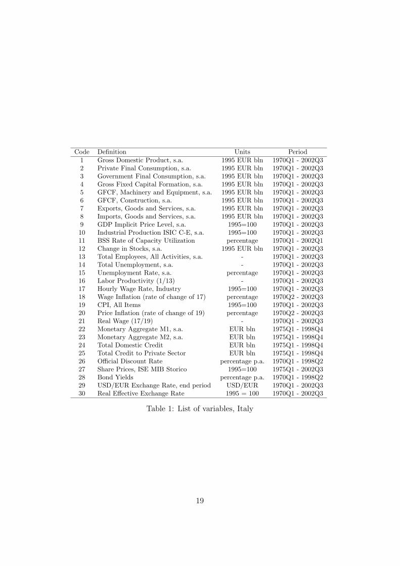
Code Definition Units Period1 Gross Domestic Product, s.a. 1995 EUR bln 1970Q1 - 2002Q32 Private Final Consumption, s.a. 1995 EUR bln 1970Q1 - 2002Q33 Government Final Consumption, s.a. 1995 EUR bln 1970Q1 - 2002Q34 Gross Fixed Capital Formation, s.a. 1995 EUR bln 1970Q1 - 2002Q35 GFCF, Machinery and Equipment, s.a. 1995 EUR bln 1970Q1 - 2002Q36 GFCF, Construction, s.a. 1995 EUR bln 1970Q1 - 2002Q37 Exports, Goods and Services, s.a. 1995 EUR bln 1970Q1 - 2002Q38 Imports, Goods and Services, s.a. 1995 EUR bln 1970Q1 - 2002Q39 GDP Implicit Price Level, s.a. 1995=100 1970Q1 - 2002Q310 Industrial Production ISIC C-E, s.a. 1995=100 1970Q1 - 2002Q311 BSS Rate of Capacity Utilization percentage 1970Q1 - 2002Q112 Change in Stocks, s.a. 1995 EUR bln 1970Q1 - 2002Q313 Total Employees, All Activities, s.a. - 1970Q1 - 2002Q314 Total Unemployment, s.a. - 1970Q1 - 2002Q315 Unemployment Rate, s.a. percentage 1970Q1 - 2002Q316 Labor Productivity (1/13) - 1970Q1 - 2002Q317 Hourly Wage Rate, Industry 1995=100 1970Q1 - 2002Q318 Wage Inflation (rate of change of 17) percentage 1970Q2 - 2002Q319 CPI, All Items 1995=100 1970Q1 - 2002Q320 Price Inflation (rate of change of 19) percentage 1970Q2 - 2002Q321 Real Wage (17/19) - 1970Q1 - 2002Q322 Monetary Aggregate M1, s.a. EUR bln 1975Q1 - 1998Q423 Monetary Aggregate M2, s.a. EUR bln 1975Q1 - 1998Q424 Total Domestic Credit EUR bln 1975Q1 - 1998Q425 Total Credit to Private Sector EUR bln 1975Q1 - 1998Q426 Official Discount Rate percentage p.a. 1970Q1 - 1998Q227 Share Prices, ISE MIB Storico 1995=100 1975Q1 - 2002Q328 Bond Yields percentage p.a. 1970Q1 - 1998Q229 USD/EUR Exchange Rate, end period USD/EUR 1970Q1 - 2002Q330 Real Effective Exchange Rate 1995 = 100 1970Q1 - 2002Q3
Table 1: List of variables, Italy
19

Code Definition Units Period1 Gross Domestic Product, s.a. 1996 USD bln 1970Q1 - 2002Q32 Private Final Consumption Expenditures, s.a. 1996 USD bln 1970Q1 - 2002Q33 Government Final Consumption Expenditures, s.a. 1996 USD bln 1970Q1 - 2002Q34 Gross Fixed Capital Formation, s.a. 1996 USD bln 1970Q1 - 2002Q35 GFCF, Machinery and Equipment, s.a. 1996 USD bln 1970Q1 - 2002Q36 GFCF, Construction, s.a. 1996 USD bln 1970Q1 - 2002Q37 Change in Stocks, s.a. 1996 USD bln 1970Q1 - 2002Q38 Exports, Goods and Services, s.a. 1996 USD bln 1970Q1 - 2002Q39 Imports, Goods and Services, s.a. 1996 USD bln 1970Q1 - 2002Q310 Industrial Production ISIC C-E, s.a. 1995=100 1970Q1 - 2002Q311 Capacity Utilization Rate, s.a. percentage 1970Q1 - 2002Q312 Civilian Employment, s.a. - 1970Q1 - 2002Q313 Unemployment Total, s.a. - 1970Q1 - 2002Q314 Unemp % Civ. Labor Force, s.a. percentage 1970Q1 - 2002Q315 Hourly Earnings, Total Private, s.a. 1995=100 1970Q1 - 2002Q316 Wage Inflation (rate of change of 15) percentage 1970Q1 - 2002Q317 CPI All Items, s.a. 1995=100 1970Q1 - 2002Q318 CPI Inflation (rate of change of 17) percentage 1970Q1 - 2002Q319 Money Supply M1, s.a. USD bln 1975Q1 - 1998Q420 Money Supply M2, s.a. USD bln 1975Q1 - 1998Q421 Commercial Banks Loans, s.a. USD bln 1975Q1 - 1998Q422 Federal Funds Rate percentage p.a. 1970Q1 - 1998Q223 Government Composite Bonds (>10 years) percentage p.a. 1970Q1 - 1998Q224 Share Prices: NYSE Common Stocks 1995=100 1975Q1 - 2002Q325 Real Effective Exchange Rate 1995 = 100 1970Q1 - 2002Q326 Real Wage (15/16) - 1970Q1 - 2002Q327 Labor Productivity (1/12) - 1970Q1 - 2002Q3
Table 2: List of variables, USA
20

Ital
yU
SAV
aria
ble
Mea
nSt
d.D
ev.
Skew
ness
Exc
.K
urt.
Mea
nSt
d.D
ev.
Skew
ness
Exc
.K
urt.
GD
P0.
0012
0.01
240.
5495
0.94
44-0
.000
10.
0157
-0.4
931
0.69
89P
riva
teFin
alC
onsu
mpt
ion
0.00
080.
0129
0.45
73-0
.262
4-0
.000
60.
0125
-0.2
596
0.16
76G
over
nmen
tFin
alC
onsu
mpt
ion
0.00
090.
0077
0.40
52-0
.274
1-0
.001
20.
0077
0.12
700.
0254
GC
FC
-0.0
005
0.02
96-0
.143
80.
1482
-0.0
011
0.04
35-0
.425
60.
0330
GC
FC
Mac
hine
ry&
Equ
ipm
ent
0.00
070.
0468
-0.3
449
0.07
670.
0007
0.04
38-0
.267
6-0
.050
8G
CFC
Con
stru
ctio
n-0
.001
00.
0232
0.02
65-0
.335
9-0
.002
00.
0474
-0.6
846
0.40
33E
xpor
ts0.
0004
0.03
110.
6593
0.14
080.
0039
0.03
730.
1770
-0.3
176
Impo
rts
0.00
060.
0416
0.08
74-0
.257
5-0
.003
60.
0477
-1.0
746
1.28
80In
dust
rial
Pro
duct
ion
0.00
230.
0314
0.11
290.
4450
0.00
040.
0301
-0.4
400
0.87
51C
hang
ein
Stoc
ks0.
5367
4.66
520.
3115
0.16
890.
7679
20.8
229
-0.0
840
0.32
41R
ate
ofC
apac
ity
Uti
lizat
ion
-0.0
015
1.58
82-0
.156
70.
5163
0.10
142.
7837
-0.4
944
0.85
73Tot
alE
mpl
oym
ent
-0.0
002
0.01
010.
9780
1.37
350.
0005
0.01
02-0
.369
90.
0397
Tot
alU
nem
ploy
men
t0.
0023
0.04
89-1
.066
4-0
.288
80.
0015
0.10
400.
3762
0.03
03U
nem
ploy
men
t%
Tot
alLab
orFo
rce
0.02
870.
3714
-0.7
042
0.16
850.
0064
0.74
760.
8075
0.66
01Lab
orP
rodu
ctiv
ity
0.00
170.
0119
0.44
760.
4434
-0.0
005
0.00
80-0
.396
31.
4132
Hou
rly
Wag
eR
ate
0.00
730.
0181
0.07
870.
2787
0.00
130.
0075
1.09
290.
7150
CP
IA
llIt
ems
0.00
370.
0185
-1.3
198
-0.6
231
0.00
200.
0147
0.13
350.
4439
Rea
lW
age
0.00
190.
0042
1.25
681.
1240
-0.0
007
0.01
070.
2965
0.55
32H
ourl
yW
age
Rat
e,(r
ate
ofch
ange
)0.
0005
0.00
560.
1557
1.35
73-0
.000
00.
0023
0.34
780.
0136
CP
IA
llIt
ems
(rat
eof
chan
ge)
0.00
050.
0048
0.43
541.
8604
0.00
030.
0040
0.67
750.
6629
M1
0.01
160.
0173
0.35
260.
6679
0.00
660.
0299
0.35
31-0
.794
5M
20.
0114
0.01
83-0
.802
51.
3530
0.00
300.
0112
-0.4
501
-0.4
161
Tot
alC
redi
tto
Pri
vate
Sect
or0.
0051
0.02
630.
3356
-0.8
368
0.00
380.
0221
-0.3
261
-0.4
424
Offi
cial
Dis
coun
tR
ate
0.05
821.
5344
-0.0
402
-0.5
742
0.09
571.
7195
0.64
95-0
.390
5B
ond
Yie
lds
0.04
931.
3112
0.55
090.
1321
0.04
270.
7740
0.40
170.
6631
Rea
lE
ffect
ive
Exc
hang
eR
ate
-0.0
015
0.03
270.
0999
-0.1
802
-0.0
044
0.03
691.
1238
-0.9
113
Shar
eP
rice
s-0
.004
70.
2125
0.54
88-0
.563
0-0
.001
40.
0685
-0.0
729
-0.5
775
Tab
le3:
Sum
mar
yst
atis
tics
ofban
dpas
sfilt
ered
Ital
ian
mac
roec
onom
icva
riab
les,
wit
hK
=12
.
21

GD
PSe
ries
t-6
t-5
t-4
t-3
t-2
t-1
tt+
1t+
2t+
3t+
4t+
5t+
6G
DP
-0.3
5-0
.21
0.04
0.36
0.67
0.91
1.00
0.91
0.67
0.36
0.04
-0.2
1-0
.35
Pri
vate
Fin
alC
onsu
mpt
ion
0.03
0.15
0.32
0.51
0.67
0.78
0.78
0.64
0.41
0.14
-0.1
2-0
.34
-0.4
8G
over
nmen
tFin
alC
onsu
mpt
ion
0.18
0.12
0.04
-0.0
4-0
.11
-0.1
5-0
.14
-0.0
9-0
.01
0.08
0.16
0.23
0.26
Gro
ssFix
edC
apit
alFo
rmat
ion
0.02
0.22
0.43
0.62
0.76
0.82
0.77
0.61
0.39
0.17
-0.0
1-0
.16
-0.2
4E
xpor
ts-0
.47
-0.4
7-0
.41
-0.3
0-0
.15
0.02
0.20
0.33
0.41
0.45
0.47
0.47
0.47
Impo
rts
-0.2
7-0
.18
-0.0
10.
220.
470.
700.
830.
820.
670.
440.
19-0
.05
-0.2
3G
FC
FM
achi
nery
&E
quip
men
t-0
.26
-0.0
80.
160.
420.
660.
840.
900.
810.
600.
350.
11-0
.09
-0.2
3G
FC
FC
onst
ruct
ion
0.45
0.63
0.73
0.73
0.65
0.49
0.28
0.05
-0.1
2-0
.22
-0.2
5-0
.24
-0.2
1In
dust
rial
Pro
duct
ion
-0.4
9-0
.35
-0.1
00.
220.
530.
790.
920.
860.
640.
360.
08-0
.15
-0.2
8C
hang
ein
Stoc
ks-0
.61
-0.5
4-0
.33
-0.0
30.
300.
600.
770.
760.
580.
320.
03-0
.21
-0.3
7R
ate
ofC
apac
ity
Uti
lizat
ion
-0.6
7-0
.57
-0.3
5-0
.04
0.30
0.61
0.82
0.86
0.75
0.56
0.36
0.19
0.08
Tot
alE
mpl
oyee
sA
llA
ctiv
itie
s0.
260.
360.
440.
510.
540.
520.
430.
260.
07-0
.11
-0.2
6-0
.38
-0.4
4U
nem
ploy
men
tTot
al-0
.51
-0.6
3-0
.64
-0.5
4-0
.34
-0.0
80.
210.
440.
550.
530.
420.
270.
11U
nem
ploy
ed%
Tot
alLab
orFo
rce
-0.5
1-0
.61
-0.6
1-0
.52
-0.3
5-0
.11
0.16
0.38
0.50
0.52
0.47
0.36
0.25
Lab
orP
rodu
ctiv
ity
-0.7
2-0
.64
-0.4
1-0
.06
0.32
0.63
0.80
0.81
0.67
0.41
0.09
-0.1
8-0
.31
CP
IA
llIt
ems
0.03
0.11
0.16
0.15
0.09
-0.0
3-0
.21
-0.3
9-0
.54
-0.6
4-0
.69
-0.6
9-0
.63
Hou
rly
Wag
eR
ate
-0.1
8-0
.12
-0.0
6-0
.02
-0.0
2-0
.09
-0.2
1-0
.35
-0.4
7-0
.56
-0.5
9-0
.56
-0.4
5C
PI
All
Item
s(r
ate
ofch
ange
)-0
.26
-0.1
50.
050.
280.
510.
650.
660.
530.
320.
09-0
.14
-0.3
2-0
.43
Hou
rly
Wag
eR
ate
(rat
eof
chan
ge)
-0.2
0-0
.21
-0.1
20.
030.
220.
380.
450.
400.
260.
05-0
.19
-0.4
1-0
.56
Rea
lW
age
-0.3
0-0
.30
-0.2
7-0
.21
-0.1
5-0
.09
-0.0
5-0
.03
-0.0
2-0
.02
0.00
0.05
0.12
M1
-0.5
1-0
.42
-0.2
7-0
.10
0.07
0.21
0.32
0.40
0.45
0.45
0.40
0.30
0.17
M2
-0.6
9-0
.64
-0.5
3-0
.37
-0.1
9-0
.01
0.15
0.29
0.41
0.48
0.49
0.44
0.32
Tot
alD
omes
tic
Cre
dit
-0.1
9-0
.24
-0.2
9-0
.34
-0.3
7-0
.41
-0.4
4-0
.47
-0.4
9-0
.49
-0.4
5-0
.37
-0.2
4Tot
alC
redi
tto
Pri
vate
Sect
or0.
320.
260.
170.
05-0
.08
-0.2
1-0
.32
-0.4
3-0
.52
-0.5
9-0
.64
-0.6
5-0
.63
Shar
eP
rice
s0.
350.
350.
300.
230.
160.
100.
050.
020.
00-0
.01
0.00
0.01
0.04
USD
/EU
R0.
250.
330.
370.
380.
370.
350.
320.
290.
270.
260.
260.
250.
20R
ealE
ffect
ive
Exc
hang
eR
ate
0.36
0.39
0.39
0.34
0.28
0.21
0.14
0.07
0.02
-0.0
2-0
.06
-0.1
2-0
.19
Offi
cial
Dis
coun
tR
ate
-0.1
0-0
.01
0.12
0.27
0.38
0.41
0.32
0.12
-0.1
4-0
.40
-0.6
2-0
.76
-0.7
7B
ond
Yie
lds
0.31
0.29
0.27
0.23
0.16
0.06
-0.0
9-0
.26
-0.4
0-0
.52
-0.5
9-0
.61
-0.5
6
Tab
le4:
Cro
ss-c
orre
lati
onco
effici
ents
ofban
dpas
s-filt
ered
vari
able
svs.
the
filt
ered
GD
P:
Ital
y.K
=12
.Bol
d:
cros
s-co
rrel
atio
ns
sign
ifica
ntl
ydiff
eren
tfr
omU
.S.on
es.
22

GD
PSe
ries
t-6
t-5
t-4
t-3
t-2
t-1
tt+
1t+
2t+
3t+
4t+
5t+
6G
DP
-0.1
6-0
.02
0.20
0.46
0.71
0.91
1,00
0.91
0.71
0.46
0.20
-0.0
2-0
.16
Pri
vate
Fin
alC
onsu
mpt
ion
-0.2
7-0
.12
0.08
0.32
0.57
0.76
0.88
0.90
0.85
0.73
0.58
0.43
0.30
Gov
ernm
ent
Fin
alC
onsu
mpt
ion
0.54
0.50
0.40
0.28
0.14
0.02
-0.0
6-0
.11
-0.1
3-0
.13
-0.1
2-0
.11
-0.1
0G
ross
Fix
edC
apit
alFo
rmat
ion
-0.1
70.
040.
290.
550.
790.
930.
960.
880.
730.
530.
330.
160.
03E
xpor
ts0.
340.
390.
450.
500.
490.
430.
310.
160.
01-0
.14
-0.2
9-0
.42
-0.5
2Im
port
s-0
.45
-0.2
40.
040.
350.
620.
790.
840.
800.
700.
590.
480.
400.
33G
FC
FM
achi
nery
&E
quip
men
t-0
.04
0.18
0.43
0.68
0.86
0.93
0.89
0.76
0.59
0.39
0.19
0.03
-0.0
9G
FC
FC
onst
ruct
ion
-0.2
6-0
.08
0.15
0.42
0.68
0.87
0.95
0.92
0.80
0.62
0.42
0.25
0.12
Cha
nge
inSt
ocks
-0.5
8-0
.49
-0.2
90.
000.
310.
550.
660.
630.
500.
320.
160.
070.
04R
ate
ofC
apac
ity
Uti
lizat
ion
-0.3
6-0
.18
0.07
0.37
0.64
0.83
0.90
0.87
0.76
0.61
0.44
0.30
0.18
Civ
ilian
Em
ploy
men
t0.
060.
250.
480.
700.
880.
950.
920.
790.
610.
400.
190.
02-0
.12
Une
mpl
oym
ent
Tot
al0.
08-0
.11
-0.3
5-0
.60
-0.8
1-0
.92
-0.9
2-0
.83
-0.6
6-0
.47
-0.2
8-0
.12
0.01
Lab
orpr
oduc
tivi
ty-0
.46
-0.3
8-0
.21
0.05
0.36
0.65
0.83
0.88
0.80
0.63
0.42
0.24
0.12
CP
IA
llIt
ems
0.37
0.27
0.14
-0.0
2-0
.19
-0.3
5-0
.50
-0.6
2-0
.71
-0.7
6-0
.77
-0.7
5-0
.69
Hou
rly
Ear
ning
sTot
alP
riva
te0.
060.
060.
050.
01-0
.05
-0.1
4-0
.24
-0.3
3-0
.41
-0.4
8-0
.53
-0.5
5-0
.52
CP
IA
llIt
ems
(rat
eof
chan
ge)
0.25
0.25
0.21
0.13
0.01
-0.1
5-0
.30
-0.4
2-0
.46
-0.4
4-0
.38
-0.3
3-0
.29
Hou
rly
Ear
ning
sTot
alP
riva
te(r
ate
ofch
ange
)-0
.05
0.12
0.25
0.28
0.22
0.11
-0.0
2-0
.11
-0.1
8-0
.24
-0.3
1-0
.40
-0.4
3R
ealW
age
-0.4
6-0
.32
-0.1
50.
030.
210.
380.
510.
600.
660.
680.
660.
610.
55M
1-0
.20
-0.2
5-0
.28
-0.2
7-0
.21
-0.1
10.
030.
160.
260.
330.
360.
370.
36M
2-0
.05
-0.1
2-0
.18
-0.2
0-0
.19
-0.1
3-0
.04
0.06
0.15
0.22
0.27
0.31
0.35
Com
mer
cial
Ban
kLoa
ns0.
520.
660.
740.
770.
710.
590.
400.
200.
02-0
.08
-0.1
2-0
.10
-0.0
9Sh
are
pric
es0.
240.
08-0
.08
-0.1
8-0
.18
-0.0
80.
090.
260.
360.
340.
230.
07-0
.06
Fede
ralFu
nds
Rat
e0.
350.
410.
480.
550.
580.
540.
430.
250.
02-0
.22
-0.4
3-0
.59
-0.6
8U
SAG
over
nmen
tco
mpo
site
bond
s(>
10ye
ars)
-0.0
20.
000.
050.
120.
160.
150.
07-0
.07
-0.2
3-0
.39
-0.5
0-0
.54
-0.5
3
Tab
le5:
Cro
ss-c
orre
lati
onco
effici
ents
ofban
dpas
s-filt
ered
vari
able
svs.
the
filt
ered
GD
P:U
SA
.K
=12
.
23

Cause GDP GDP CausedSeries F-stat F-statPrivate Final Consumption 5.230 2.308
(0.000) (0.051)
Government Final Consumption 1.006 1.386(0.419) (0.237)
Gross Fixed Capital Formation 0.938 2.001(0.460) (0.086)
Exports 2.599 2.478(0.030) (0.038)
Imports 1.053 2.195(0.392) (0.062)
GFCF Machinery and Equipment 2.805 3.048(0.021) (0.014)
GFCF Construction 0.919 5.066(0.472) (0.000)
Industrial Production 1.470 2.607(0.207) (0.030)
Change in Stocks 3.731 1.880(0.004) (0.105)
Rate of Capacity Utilization 1.722 4.577(0.138) (0.001)
Total Employees All Activities 1.946 1.922(0.094) (0.098)
Unemployment Total 1.987 1.356(0.088) (0.248)
Unemployed % Total Labour Force 1.433 1.283(0.220) (0.278)
Labor Productivity 2.072 1.641(0.076) (0.157)
CPI All Items 3.104 4.998(0.012) (0.000)
Hourly Wage Rate 3.220 3.324(0.010) (0.008)
CPI All Items (rate of change) 3.185 4.869(0.011) (0.001)
Hourly Wage Rate (rate of change) 2.502 4.840(0.036) (0.001)
Real Wage 1.527 0.956(0.189) (0.449)
M1 1.986 3.168(0.095) (0.014)
M2 2.563 2.257(0.037) (0.061)
Total Domestic Credit 2.768 0.404(0.026) (0.844)
Total Credit to Private Sector 2.461 0.780(0.044) (0.568)
Share Prices 0.659 0.238(0.656) (0.944)
USD/EUR 2.615 1.874(0.030) (0.107)
Real Effective Exchange Rate 0.685 0.468(0.636) (0.799)
Official Discount Rate 2.137 3.415(0.070) (0.008)
Bond Yields 0.855 0.382(0.515) (0.860)
Table 6: Granger causality tests, bivariate models with each variable and theGDP, and five lags: Italy. K = 12. p-values are in brackets. Bold : valuesfor which the null (no causality) is rejected at 5%-significance level.
24

Cause GDP GDP CausedSeries F-stat F-statPrivate Final Consumption 2.595 2.530
(0.031) (0.034)
Government Final Consumption 3.172 2.556(0.011) (0.033)
GFCF 1.434 3.644(0.220) (0.005)
Exports 0.984 5.536(0.432) (0.000)
Imports 1.128 2.115(0.351) (0.071)
GFCF Machinery and Equipment 1.008 1.291(0.418) (0.275)
GFCF Construction 4.991 4.947(0.000) (0.000)
Change in Stocks 2.530 5.347(0.034) (0.000)
Rate of Capacity Utilization 4.103 0.988(0.002) (0.429)
Civilian Employment 3.622 3.192(0.005) (0.011)
Unemployment Total 5.082 2.020(0.000) (0.083)
Labor productivity 3.621 3.069(0.005) (0.013)
CPI All Items 3.971 3.771(0.003) (0.004)
Hourly Earnings Total Private 3.842 1.887(0.003) (0.104)
CPI All Items (rate of change) 2.234 6.827(0.058) (0.000)
Hourly Earnings Total Private (rate of change) 3.758 3.165(0.004) (0.011)
Real Wage 3.375 0.648(0.008) (0.664)
M1 3.798 2.792(0.005) (0.025)
M2 2.388 1.136(0.049) (0.352)
Commercial Bank Loans 4.822 2.093(0.001) (0.080)
Share prices 0.615 1.025(0.688) (0.409)
Federal Funds Rate 4.287 2.691(0.002) (0.027)
USA Government composite bonds (>10 years) 5.348 0.822(0.000) (0.538)
Table 7: Granger causality tests, bivariate models with each variable and theGDP, and five lags: U.S. K = 12. p-values are in brackets. Bold : values forwhich the null (no causality) is rejected at 5%-significance level.
25

−6 −5 −4 −3 −2 −1 0 1 2 3 4 5 6−0.5
0
0.5
1 GDP
−6 −5 −4 −3 −2 −1 0 1 2 3 4 5 6−0.5
0
0.5
1Private Final Consumption
−6 −5 −4 −3 −2 −1 0 1 2 3 4 5 6−0.5
0
0.5
1Government Final Consumption
−6 −5 −4 −3 −2 −1 0 1 2 3 4 5 6−0.5
0
0.5
1Gross Fixed Capital Formation
−6 −5 −4 −3 −2 −1 0 1 2 3 4 5 6−0.5
0
0.5
1 Exports
−6 −5 −4 −3 −2 −1 0 1 2 3 4 5 6−0.5
0
0.5
1 Imports
Figure 1: Cross-correlograms, Italian data: GDP components.Diamonds: GDP autocorrelation. Squares: GDP component.
26

−6 −5 −4 −3 −2 −1 0 1 2 3 4 5 6−0.5
0
0.5
1Gross Fixed Capital Formation
−6 −5 −4 −3 −2 −1 0 1 2 3 4 5 6−0.5
0
0.5
1GFCF Machinery & Equipment
−6 −5 −4 −3 −2 −1 0 1 2 3 4 5 6−0.5
0
0.5
1GFCF Construction
Figure 2: Cross-correlograms, Italian data: investment components.Diamonds: GDP autocorrelation. Squares: investment component.
27

−6 −5 −4 −3 −2 −1 0 1 2 3 4 5 6−0.5
0
0.5
1Industrial Production
−6 −5 −4 −3 −2 −1 0 1 2 3 4 5 6−1
−0.5
0
0.5
1Change in Stocks
−6 −5 −4 −3 −2 −1 0 1 2 3 4 5 6−1
−0.5
0
0.5
1Rate of Capacity Utilization
Figure 3: Cross-correlograms, Italian data: production variables.Diamonds: GDP autocorrelation. Squares: production variable.
28

−6 −5 −4 −3 −2 −1 0 1 2 3 4 5 6−0.5
0
0.5
1Total Employees All Activities
−6 −5 −4 −3 −2 −1 0 1 2 3 4 5 6−1
−0.5
0
0.5
1Unemployment Total
−6 −5 −4 −3 −2 −1 0 1 2 3 4 5 6−1
−0.5
0
0.5
1Unemployed % Total Labour Force
−6 −5 −4 −3 −2 −1 0 1 2 3 4 5 6−1
−0.5
0
0.5
1Labor Productivity
Figure 4: Cross-correlograms, Italian data: labor market variables.Diamonds: GDP autocorrelation. Squares: labor market variable.
29

−6−5−4−3−2−1 0 1 2 3 4 5 6−1
−0.5
0
0.5
1 CPI All Items
−6−5−4−3−2−1 0 1 2 3 4 5 6−1
−0.5
0
0.5
1 Hourly Wage Rate
−6−5−4−3−2−1 0 1 2 3 4 5 6−0.5
0
0.5
1CPI All Items (rate of change)
−6−5−4−3−2−1 0 1 2 3 4 5 6−1
−0.5
0
0.5
1Hourly Wage Rate (rate of change)
−6−5−4−3−2−1 0 1 2 3 4 5 6−0.5
0
0.5
1 Real Wage
Figure 5: Cross-correlograms, Italian data: prices and wages.Diamonds: GDP autocorrelation. Squares: prices and wages variable.
30

−6 −5 −4 −3 −2 −1 0 1 2 3 4 5 6−1
−0.5
0
0.5
1 M1
−6 −5 −4 −3 −2 −1 0 1 2 3 4 5 6−1
−0.5
0
0.5
1 M2
−6 −5 −4 −3 −2 −1 0 1 2 3 4 5 6−0.5
0
0.5
1 Total Domestic Credit
−6 −5 −4 −3 −2 −1 0 1 2 3 4 5 6−1
−0.5
0
0.5
1 Total Credit to Private Sector
−6 −5 −4 −3 −2 −1 0 1 2 3 4 5 6−0.5
0
0.5
1 Share Prices
−6 −5 −4 −3 −2 −1 0 1 2 3 4 5 6−0.5
0
0.5
1 USD/EUR
−6 −5 −4 −3 −2 −1 0 1 2 3 4 5 6−1
−0.5
0
0.5
1 Official Discount Rate
−6 −5 −4 −3 −2 −1 0 1 2 3 4 5 6−1
−0.5
0
0.5
1 Bond Yields
Figure 6: Cross-correlograms, Italian data: monetary and financial variables.Diamonds: GDP autocorrelation. Squares: monetary and financial variable.
31

−6 −5 −4 −3 −2 −1 0 1 2 3 4 5 6−0.5
0
0.5
1 GDP
−6 −5 −4 −3 −2 −1 0 1 2 3 4 5 6−0.5
0
0.5
1Private Final Consumption
−6 −5 −4 −3 −2 −1 0 1 2 3 4 5 6−0.4
−0.2
0
0.2
0.4
0.6Government Final Consumption
−6 −5 −4 −3 −2 −1 0 1 2 3 4 5 6−0.5
0
0.5
1Gross Fixed Capital Formation
−6 −5 −4 −3 −2 −1 0 1 2 3 4 5 6−1
−0.5
0
0.5 Exports
−6 −5 −4 −3 −2 −1 0 1 2 3 4 5 6−0.5
0
0.5
1 Imports
Figure 7: Cross-correlograms, Italian ad U.S. data: GDP components.Squares: Italian data. Asterisks: U.S. data. Diamonds: Stock and Wat-son data.
32
−6 −5 −4 −3 −2 −1 0 1 2 3 4 5 6−0.4
−0.2
0
0.2
0.4
0.6
0.8
1GFCF Machinery & Equipment
−6 −5 −4 −3 −2 −1 0 1 2 3 4 5 6−0.4
−0.2
0
0.2
0.4
0.6
0.8
1GFCF Construction
−6 −5 −4 −3 −2 −1 0 1 2 3 4 5 6−0.8
−0.6
−0.4
−0.2
0
0.2
0.4
0.6
0.8Change in Stocks
−6 −5 −4 −3 −2 −1 0 1 2 3 4 5 6−0.8
−0.6
−0.4
−0.2
0
0.2
0.4
0.6
0.8
1Rate of Capacity Utilization
Figure 8: Cross-correlograms, Italian ad U.S. data: production variablesand investment components. Squares: Italian data. Asterisks: U.S. data.Diamonds: Stock and Watson data.
33

−6 −5 −4 −3 −2 −1 0 1 2 3 4 5 6−0.5
0
0.5
1Total Employees All Activities
−6 −5 −4 −3 −2 −1 0 1 2 3 4 5 6−1
−0.5
0
0.5
1Unemployment Total
−6 −5 −4 −3 −2 −1 0 1 2 3 4 5 6−1
−0.5
0
0.5
1Labor Productivity
Figure 9: Cross-correlograms, Italian ad U.S. data: labor market variables.Squares: Italian data. Asterisks: U.S. data. Diamonds: Stock and Watsondata.
34

−6−5 −4 −3−2 −1 0 1 2 3 4 5 6−1
−0.5
0
0.5 CPI All Items
−6−5 −4 −3−2 −1 0 1 2 3 4 5 6−1
−0.5
0
0.5
1 Hourly Wage Rate
−6−5 −4 −3−2 −1 0 1 2 3 4 5 6−0.5
0
0.5
1CPI All Items (rate of change)
−6−5 −4 −3−2 −1 0 1 2 3 4 5 6−1
−0.5
0
0.5
1Hourly Wage Rate (rate of change)
−6−5 −4 −3−2 −1 0 1 2 3 4 5 6−0.4
−0.2
0
0.2
0.4
0.6 Real Wage
Figure 10: Cross-correlograms, Italian ad U.S. data: prices and wages.Squares: Italian data. Asterisks: U.S. data. Diamonds: Stock and Wat-son data.
35

−6 −5 −4 −3 −2 −1 0 1 2 3 4 5 6−1
−0.5
0
0.5 M1
−6 −5 −4 −3 −2 −1 0 1 2 3 4 5 6−1
−0.5
0
0.5
1 M2
−6 −5 −4 −3 −2 −1 0 1 2 3 4 5 6−1
−0.5
0
0.5
1Total Credit to Private Sector
−6 −5 −4 −3 −2 −1 0 1 2 3 4 5 6−0.4
−0.2
0
0.2
0.4
0.6Share Prices
−6 −5 −4 −3 −2 −1 0 1 2 3 4 5 6−1
−0.5
0
0.5
1Official Discount Rate
−6 −5 −4 −3 −2 −1 0 1 2 3 4 5 6−1
−0.5
0
0.5Bond Yields
Figure 11: Cross-correlograms, Italian ad U.S. data: monetary and financialvariables. Squares: Italian data. Asterisks: U.S. data. Diamonds: Stockand Watson data.
36