Embed Size (px)
Citation preview
Emerging Economy Business Cycles: Financial Integration and Terms of Trade
Shocks
Prepared by Rudrani Bhattacharya,Ila Patnaik, Madhavi Pundit
WP/13/119
© 2013 International Monetary Fund WP/13/119
IMF Working Paper
Research Department
Emerging Economy Business Cycles: Financial Integration and Terms of Trade Shocks
Prepared by Ila Patnaik, Rudrani Bhattacharya, Madhavi Pundit1
Authorized for distribution by Prakash Loungani
May 2013
Abstract
This paper analyses the extent to which financial integration impacts the manner in which terms of trade affect business cycles in emerging economies. Using a s mall open economy model, we show that as capital account openness increases in an economy that faces trade shocks, business cycle volatility reduces. For an economy with limited financial openness, and a relatively open trade account, a model with exogenous terms of trade shocks is able to replicate the features of the business cycle.
JEL Classification Numbers: F4, E32
Keywords: Macroeconomics, real business cycles, emerging market DSGE models, volatility, terms of trade.
Authors E-Mail Addresses: [email protected]; [email protected]; [email protected]
1 Visiting Scholar, Research Department; National Institute of Public Finance and Policy, India; and Asian Development Bank, Philippines respectively.
This Working Paper should not be reported as representing the views of the IMF. The views expressed in this Working Paper are those of the author(s) and do not necessarily represent those of the IMF or IMF policy. Working Papers describe research in progress by the author(s) and are published to elicit comments and to further debate.
2
Contents
1 Introduction 3
2 Openness in emerging markets 52.1 Financial versus trade openness . . . . . . . . . . . . . . . . . . . . 62.2 Relative volatility of the terms of trade . . . . . . . . . . . . . . . . 72.3 Current account volatility . . . . . . . . . . . . . . . . . . . . . . . 8
3 Case of India 93.1 Limited financial openness . . . . . . . . . . . . . . . . . . . . . . . 93.2 Role of terms of trade . . . . . . . . . . . . . . . . . . . . . . . . . 10
4 Model 12
5 Calibration 15
6 Results 176.1 Financial openness and volatility . . . . . . . . . . . . . . . . . . . 176.2 Business cycle features of an emerging economy . . . . . . . . . . . 19
7 Conclusion 21
3
1 Introduction
Emerging economies differ in the extent of international trade and financial inte-gration. While most emerging economies have opened their trade accounts, theyhave retained different degrees of control over their capital accounts. The interna-tional business cycle literature suggests that financial integration may play a rolein determining the volatility of domestic business cycles in an emerging economy invarious ways. The composition, magnitude and the cyclicality of capital flows maydetermine how financial openness impacts macroeconomic variables. On the otherhand, financially closed economies may be unable to share risk which again affectsdomestic volatility. Therefore, financial integration may affect the extent to whicheconomies are able to absorb external shocks (Cakici, 2011; Buch et al., 2005; vonHagen and Zhang, 2006; Levchenko, 2004)
In this paper, we study one aspect of this relation, namely the role of the levelof financial openness on the propagation of an exogenous terms of trade (tot)shock on business cycle volatility in an emerging economy. A country with anopen current account, but closed capital account is likely to have lower ability toabsorb tot shocks. This is because if trade has to balance in each period, currentaccount volatility will be low, and a shock is expected to propagate to output,consumption and investment. On the other hand, when the capital account isopen, agents can borrow and lend in international financial markets to smooththeir consumption. They are less constrained and do not need to balance the tradeaccount in each period. External tot shocks may be absorbed and not transmittedto macroeconomic variables. Hence higher terms of trade volatility is expected tolead to higher volatility of output in an economy with low capital account openness.
As emerging economies are being exposed to international markets, a body of lit-erature is developing recently on the relation between integration and volatility.For example, Kose et al. (2003) and Evans and Hnatkovska (2007) study the im-pact of financial integration in stabilizing the business cycle volatility of emergingmarkets. We extend this literature by highlighting the role that financial integra-tion could play in determining the volatility of domestic macroeconomic variables,in the presence of an exogenous terms of trade shock. Being commodity traders,emerging economies face exogenous price shocks in the world market which deter-mine domestic business cycle fluctuations (Mendoza, 1995; Kose, 2002). This papercontributes further to this discussion by examining differences in the response ofdifferent emerging economies to terms of trade shocks, and proposing a model forunderstanding how these shocks are propagated.
The model embodies features of an emerging economy and is related to the recentliterature studying emerging economy business cycles, especially those focussingon external shocks. A strand of literature studies shocks in the financial marketsdue to an open capital account. Neumeyer and Perri (2005) relate interest ratefluctuations in international financial markets to the business cycle of emergingmarkets. Uribe and Yue (2006) find that besides interest rate shocks, fluctuationsin the country spread can explain the business cycle. Based on this, Garcıa-Cicco
4
et al. (2010) and Chang and Fernandez (2010) show that the business cycle in anopen emerging economy is driven by external shocks to the country’s interest ratepremium in conjunction with financial frictions. These models, however, do notadequately explain features of the business cycle, especially the lower volatility ofthe trade balance to output ratio relative to the volatility of output seen in thedata.
Data shows that emerging economies exhibit heterogeneity in the nature of open-ness. We compare the level of trade openness (gross trade as a percent to gdp) andfinancial openness (external assets and liabilities as a percent to gdp) for a groupof emerging economies. We find a wide range in the degree of trade versus financialopenness. In general, while Asian economies have higher relative trade openness,Latin American countries have lower relative trade openness and are more finan-cially open. Further, by looking at the relation between the nature of openness andthe terms of trade fluctuations, we observe that in countries which have limitedcapital openness and more open trade accounts, the ratio of tot volatility to out-put volatility is lower. This motivates the hypothesis that financial openness playsa role in the relation between tot shocks and business cycle volatility.
We present a small open economy real business cycle model. In the model, we varythe level of financial integration from full capital mobility to financial autarky. Inaddition to a productivity shock, we incorporate shocks to the terms of trade as inMendoza (1995) and Lubik and Teo (2005).
The model is used to analyse the effect of financial integration in two ways: first,we calibrate the model using the parameters of an emerging economy, India, andvary the level of financial integration. We compare the volatility of the businesscycle obtained in the economy by assuming increasing levels of financial integra-tion. In the second approach, we calibrate the model to another emerging economy,Brazil, that is similar in most respects, especially in its exposure to terms of tradefluctuations, but is different in the level of financial integration. We compare theperformance of the model in its ability to replicate moments from the data for thetwo economies.
In the first exercise, our results show that the level of financial integration plays arole in the relation between terms of trade shocks and the business cycle volatility.We find that as financial integration increases, volatility of output, consumptionand investment declines and the volatility of trade balance to output increases.This is because with higher financial integration, the economy is not constrainedin having to balance its current account every period. Volatility in terms of tradedoes not get transmitted to output, consumption and investment.
We also see that the model broadly matches the features of an emerging economy,India, characterised by trade openness but limited financial openness. It reproducesthe relatively higher consumption volatility, countercyclical trade balance, and thelower relative volatility of trade balance to output. In the case of an economy withhigh financial openness, Brazil, the model is able to replicate the higher relativevolatility of trade balance to output.
5
Our conclusion that financial openness determines the extent to which a tot shockis transmitted to the domestic business cycle has important policy implications. Inthe face of external shocks, capital account openness enables an emerging economyto borrow and lend in the international financial markets and absorb such shocks,and thereby stabilise business cycle volatility.
The rest of the paper is organised as follows: Section 2 documents empiricallyheterogeneity in openness in emerging countries, the relation to terms of tradevolatility and current account volatility. Section 3 uses the example of India todiscuss the potential role for terms of trade shocks in explaining the business cycleof an emerging economy. Section 4 discusses a small open economy model withfinancial integration, and productivity and tot shocks, and Section 5 calibratesit to an emerging economy. Section 6 discusses the results by varying the level offinancial integration and comparing the moments from the model and the data foremerging economies. Section 7 concludes.
2 Openness in emerging markets
One of the critical features in which emerging economy business cycles differ fromthose of advanced economies is the impact of external shocks on the economy and theconsequent volatility of macroeconomic variables. The timing, pace and manner ofglobalisation of emerging economies has varied. In general, in a number of emergingeconomies, trade openness was undertaken before the capital account was opened.
The reduction in trade barriers depended on the domestic growth environmentand development policies and has thus varied across countries. Similarly, differentemerging markets opened up their capital accounts at different times and to avarying extent. Many countries still have a number of capital controls in placewhich restricts their financial openness (Chinn and Ito, 2008; Schindler, 2009; Laneand Milesi-Feretti, 2007). Table 1 presents evidence on the nature of openness forselected emerging economies.1
In this setting it is possible to see that the degree of financial openness may deter-mine the extent to which external shocks, such as trade shocks, influence macroe-conomic volatility in an emerging economy. An open capital account would allowa country to borrow, and import, even when terms of trade move against it, so asto smooth consumption. A country with a relatively closed capital account wouldnot be able to borrow and would have to absorb a tot shock by adjusting quanti-ties of exports and imports, such that the current account is more or less balanced(i.e., exports pay for its imports) every period. In the extreme, with financial au-tarky, a country must have a zero current account deficit and zero volatility of thecurrent account. Changes in the quantities of exports and imports would result inadjustments in output, investment and consumption, and in this way the tot shockpropagates to the macroeconomic variables. On the other hand, borrowing would
1The emerging markets considered are based on the msci country list, with the addition ofArgentina.
6
allow a country to have higher volatility of the current account in the face of tradeshocks, and such a shock would not propagate to the real variables. Thus, higherterms of trade volatility would lead to higher volatility of output in an economywith low capital account openness.
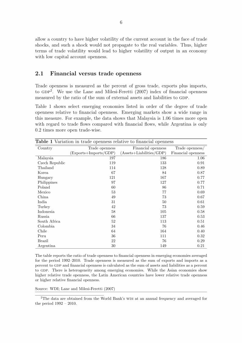
2.1 Financial versus trade openness
Trade openness is measured as the percent of gross trade, exports plus imports,to gdp2. We use the Lane and Milesi-Feretti (2007) index of financial opennessmeasured by the ratio of the sum of external assets and liabilities to gdp.
Table 1 shows select emerging economies listed in order of the degree of tradeopenness relative to financial openness. Emerging markets show a wide range inthis measure. For example, the data shows that Malaysia is 1.06 times more openwith regard to trade flows compared with financial flows, while Argentina is only0.2 times more open trade-wise.
Table 1 Variation in trade openness relative to financial openness
Country Trade openness Financial openness Trade openness/(Exports+Imports/GDP) (Assets+Liabilities/GDP) Financial openness
Malaysia 197 186 1.06Czech Republic 119 133 0.91Thailand 114 128 0.89Korea 67 84 0.87Hungary 121 167 0.77Philippines 97 127 0.77Poland 60 86 0.71Mexico 53 77 0.69China 49 73 0.67India 31 50 0.61Turkey 42 73 0.59Indonesia 58 105 0.58Russia 66 137 0.53South Africa 52 113 0.51Colombia 34 76 0.46Chile 64 164 0.40Peru 36 111 0.32Brazil 22 76 0.29Argentina 30 149 0.21
The table reports the ratio of trade openness to financial openness in emerging economies averagedfor the period 1992–2010. Trade openness is measured as the sum of exports and imports as apercent to gdp and financial openness is calculated as the sum of assets and liabilities as a percentto gdp. There is heterogeneity among emerging economies. While the Asian economies showhigher relative trade openness, the Latin American countries have lower relative trade opennessor higher relative financial openness.
Source: WDI; Lane and Milesi-Feretti (2007)
2The data are obtained from the World Bank’s wdi at an annual frequency and averaged forthe period 1992 – 2010.
7
We observe that the south, east and south-east Asian countries, namely Malaysia,Thailand, Korea, Philippines, China and India have more open trade accounts com-pared to financial accounts. In contrast, Latin American countries, such as Colom-bia, Chile, Peru, Brazil and Argentina have less relative openness in trade. Mexico,Turkey and Indonesia are similar to India with about 0.6 times more openness intrade than financial flows. While the Czech Republic, Hungary and Poland showhigher relative trade openness, Russia and South Africa appear lower in the order.In general, there is significant heterogeneity in the degree of trade openness relativeto financial openness among emerging economies.
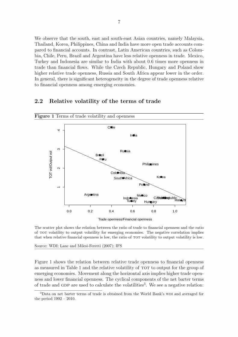
2.2 Relative volatility of the terms of trade
Figure 1 Terms of trade volatility and openness
●
●
●
●
●
●
●
●
●
●
●●
●
●
●
●●
●
0.0 0.2 0.4 0.6 0.8 1.0
12
34
Trade openness/Financial openness
TOT
vol
/Out
put v
ol Russia
Chile
Peru
India
ColombiaKorea
Brazil
Philippines
Argentina
South Africa
ThailandIndonesia
Poland
Mexico
TurkeyCzech Republic
MalaysiaHungary
The scatter plot shows the relation between the ratio of trade to financial openness and the ratioof tot volatility to output volatility for emerging economies. The negative correlation impliesthat when relative financial openness is low, the ratio of tot volatility to output volatility is low.
Source: WDI; Lane and Milesi-Feretti (2007); IFS
Figure 1 shows the relation between relative trade openness to financial opennessas measured in Table 1 and the relative volatility of tot to output for the group ofemerging economies. Movement along the horizontal axis implies higher trade open-ness and lower financial openness. The cyclical components of the net barter termsof trade and gdp are used to calculate the volatilities3. We see a negative relation:
3Data on net barter terms of trade is obtained from the World Bank’s wdi and averaged forthe period 1992 – 2010.
8
countries with more closed capital accounts and higher relative trade openness havea lower ratio of tot volatility to output volatility.
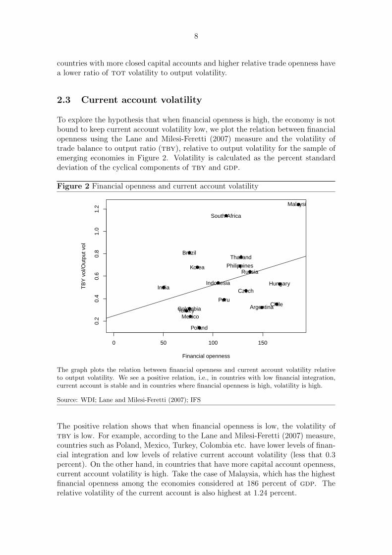
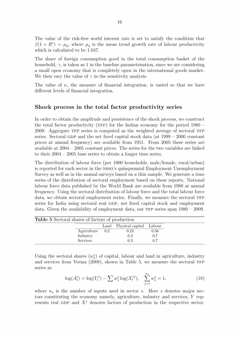
2.3 Current account volatility
To explore the hypothesis that when financial openness is high, the economy is notbound to keep current account volatility low, we plot the relation between financialopenness using the Lane and Milesi-Feretti (2007) measure and the volatility oftrade balance to output ratio (tby), relative to output volatility for the sample ofemerging economies in Figure 2. Volatility is calculated as the percent standarddeviation of the cyclical components of tby and gdp.
Figure 2 Financial openness and current account volatility
●
●
●
●
●
●
●
●
●
●
●
●
●
●
●
●
●
●
0 50 100 150
0.2
0.4
0.6
0.8
1.0
1.2
Financial openness
TB
Y v
ol/O
utpu
t vol
Malaysia
Czech
Thailand
Korea
Hungary
Philippines
Poland
Mexico
India
Turkey
Indonesia
Russia
South Africa
ColombiaChile
Peru
Brazil
Argentina
The graph plots the relation between financial openness and current account volatility relativeto output volatility. We see a positive relation, i.e., in countries with low financial integration,current account is stable and in countries where financial openness is high, volatility is high.
Source: WDI; Lane and Milesi-Feretti (2007); IFS
The positive relation shows that when financial openness is low, the volatility oftby is low. For example, according to the Lane and Milesi-Feretti (2007) measure,countries such as Poland, Mexico, Turkey, Colombia etc. have lower levels of finan-cial integration and low levels of relative current account volatility (less that 0.3percent). On the other hand, in countries that have more capital account openness,current account volatility is high. Take the case of Malaysia, which has the highestfinancial openness among the economies considered at 186 percent of gdp. Therelative volatility of the current account is also highest at 1.24 percent.
9
3 Case of India
India is an example of an emerging economy with trade openness and low financialopenness. By studying the nature of current account volatility, we provide evidencefor the potential role of tot shocks in propagating the business cycle.
3.1 Limited financial openness
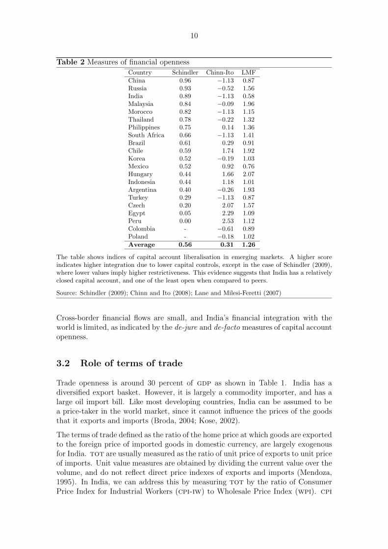
India has a large and complex structure of legal and administrative controls thatrestrict the flow of capital in the economy (Patnaik and Shah, 2011). Variousmeasures of de-jure capital controls such as Chinn and Ito (2008); Abiad et al.(2008); Quinn and Toyoda (2007) show that India has a relatively closed capitalaccount. As shown in Table 2, this not only implies that India is financially lessopen, but it is one of the least open among other emerging markets.
A measure of de-jure restrictions at a more disaggregate level of financial transac-tions is provided by Schindler (2009). The main categories in this dataset, which arefurther divided into sub-categories are: Shares or other securities of a participatingnature; Bonds or other debt securities; Money market instruments; Collective in-vestments; Financial credits; and Direct investment. According to this measure, 0implies no restrictions, while 1 implies complete restrictions in the categories. Indiafeatures high in the list among emerging markets, with an average restriction indexbetween 1995 – 2005 of 0.89.
The last column of Table 2 shows a measure of de-facto capital account opennessusing the Lane and Milesi-Ferreti database. This index is constructed based ona country’s external assets and liabilities. Lane and Milesi-Feretti (2007) describethe methodology for the construction of the index. Accordingly, international hold-ings and transactions are classified as: Portfolio investment, subdivided into eq-uity securities and debt securities; Foreign direct investment; Other investment,which includes debt instruments such as loans, deposits, and trade credits; Finan-cial derivatives; and Reserve assets. The average index for India from 2000 – 2007stands at 0.58, which again is one of the lowest among the emerging markets, andshows low level of financial integration.
10
Table 2 Measures of financial openness
Country Schindler Chinn-Ito LMFChina 0.96 −1.13 0.87Russia 0.93 −0.52 1.56India 0.89 −1.13 0.58Malaysia 0.84 −0.09 1.96Morocco 0.82 −1.13 1.15Thailand 0.78 −0.22 1.32Philippines 0.75 0.14 1.36South Africa 0.66 −1.13 1.41Brazil 0.61 0.29 0.91Chile 0.59 1.74 1.92Korea 0.52 −0.19 1.03Mexico 0.52 0.92 0.76Hungary 0.44 1.66 2.07Indonesia 0.44 1.18 1.01Argentina 0.40 −0.26 1.93Turkey 0.29 −1.13 0.87Czech 0.20 2.07 1.57Egypt 0.05 2.29 1.09Peru 0.00 2.53 1.12Colombia - −0.61 0.89Poland - −0.18 1.02Average 0.56 0.31 1.26
The table shows indices of capital account liberalisation in emerging markets. A higher scoreindicates higher integration due to lower capital controls, except in the case of Schindler (2009),where lower values imply higher restrictiveness. This evidence suggests that India has a relativelyclosed capital account, and one of the least open when compared to peers.
Source: Schindler (2009); Chinn and Ito (2008); Lane and Milesi-Feretti (2007)
Cross-border financial flows are small, and India’s financial integration with theworld is limited, as indicated by the de-jure and de-facto measures of capital accountopenness.
3.2 Role of terms of trade
Trade openness is around 30 percent of gdp as shown in Table 1. India has adiversified export basket. However, it is largely a commodity importer, and has alarge oil import bill. Like most developing countries, India can be assumed to bea price-taker in the world market, since it cannot influence the prices of the goodsthat it exports and imports (Broda, 2004; Kose, 2002).
The terms of trade defined as the ratio of the home price at which goods are exportedto the foreign price of imported goods in domestic currency, are largely exogenousfor India. tot are usually measured as the ratio of unit price of exports to unit priceof imports. Unit value measures are obtained by dividing the current value over thevolume, and do not reflect direct price indexes of exports and imports (Mendoza,1995). In India, we can address this by measuring tot by the ratio of ConsumerPrice Index for Industrial Workers (cpi-iw) to Wholesale Price Index (wpi). cpi
11
contains tradeables and non-tradeables prices and can be considered a proxy forthe home price. wpi reflects global prices of tradeables and the fluctuations of therupee, due to a large share of tradeables in it (Patnaik et al., 2011). This priceindex can be used as a proxy for foreign price.
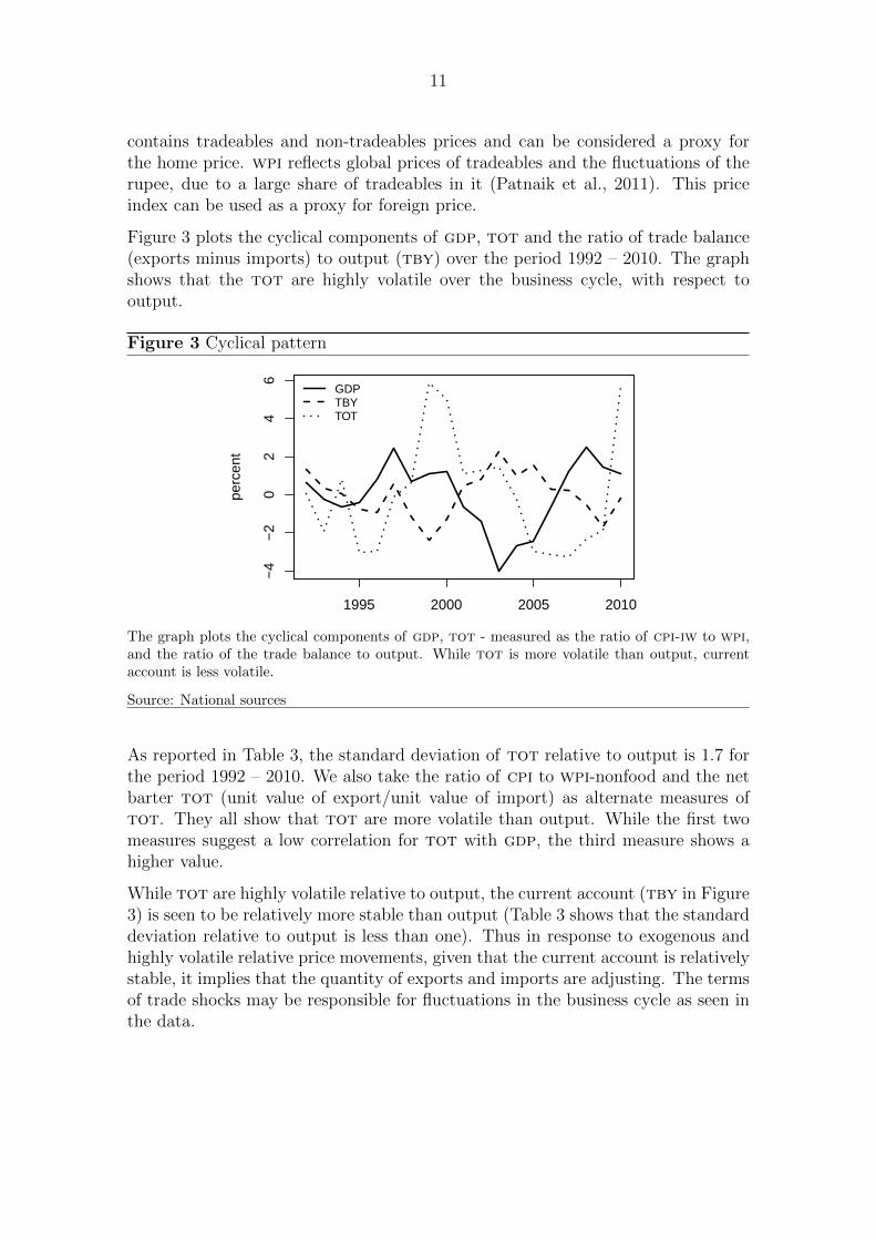
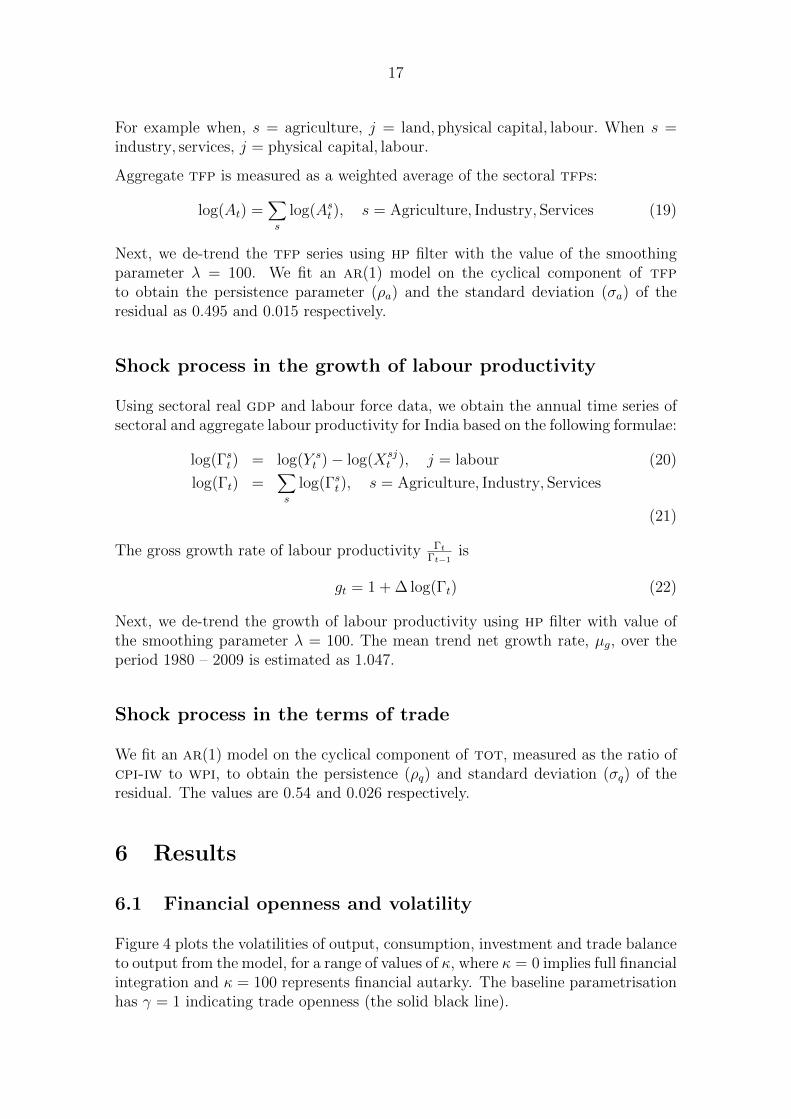
Figure 3 plots the cyclical components of gdp, tot and the ratio of trade balance(exports minus imports) to output (tby) over the period 1992 – 2010. The graphshows that the tot are highly volatile over the business cycle, with respect tooutput.
Figure 3 Cyclical pattern
1995 2000 2005 2010
−4
−2
02
46
perc
ent
GDPTBYTOT
The graph plots the cyclical components of gdp, tot - measured as the ratio of cpi-iw to wpi,and the ratio of the trade balance to output. While tot is more volatile than output, currentaccount is less volatile.
Source: National sources
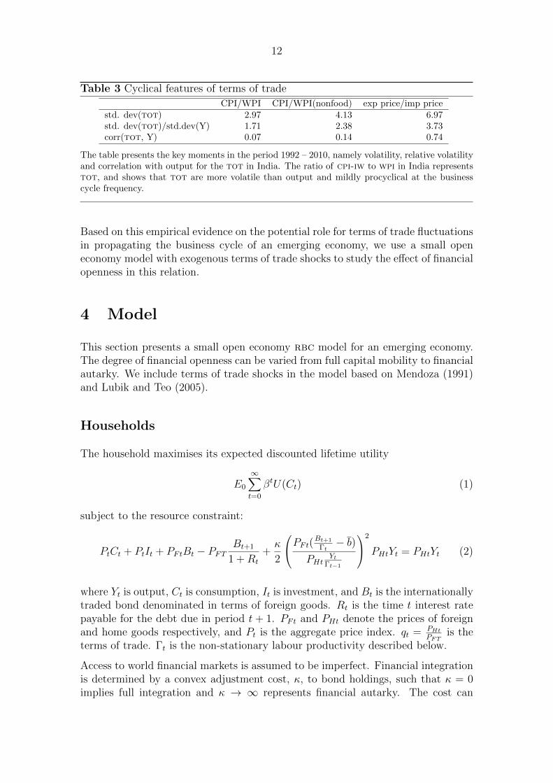
As reported in Table 3, the standard deviation of tot relative to output is 1.7 forthe period 1992 – 2010. We also take the ratio of cpi to wpi-nonfood and the netbarter tot (unit value of export/unit value of import) as alternate measures oftot. They all show that tot are more volatile than output. While the first twomeasures suggest a low correlation for tot with gdp, the third measure shows ahigher value.
While tot are highly volatile relative to output, the current account (tby in Figure3) is seen to be relatively more stable than output (Table 3 shows that the standarddeviation relative to output is less than one). Thus in response to exogenous andhighly volatile relative price movements, given that the current account is relativelystable, it implies that the quantity of exports and imports are adjusting. The termsof trade shocks may be responsible for fluctuations in the business cycle as seen inthe data.
12
Table 3 Cyclical features of terms of trade
CPI/WPI CPI/WPI(nonfood) exp price/imp pricestd. dev(tot) 2.97 4.13 6.97std. dev(tot)/std.dev(Y) 1.71 2.38 3.73corr(tot, Y) 0.07 0.14 0.74
The table presents the key moments in the period 1992 – 2010, namely volatility, relative volatilityand correlation with output for the tot in India. The ratio of cpi-iw to wpi in India representstot, and shows that tot are more volatile than output and mildly procyclical at the businesscycle frequency.
Based on this empirical evidence on the potential role for terms of trade fluctuationsin propagating the business cycle of an emerging economy, we use a small openeconomy model with exogenous terms of trade shocks to study the effect of financialopenness in this relation.
4 Model
This section presents a small open economy rbc model for an emerging economy.The degree of financial openness can be varied from full capital mobility to financialautarky. We include terms of trade shocks in the model based on Mendoza (1991)and Lubik and Teo (2005).
Households
The household maximises its expected discounted lifetime utility
E0
∞∑t=0
βtU(Ct) (1)
subject to the resource constraint:
PtCt + PtIt + PFtBt − PFTBt+1
1 +Rt
+κ
2
PFt(Bt+1
Γt− b)
PHtYt
Γt−1
2
PHtYt = PHtYt (2)
where Yt is output, Ct is consumption, It is investment, and Bt is the internationallytraded bond denominated in terms of foreign goods. Rt is the time t interest ratepayable for the debt due in period t + 1. PFt and PHt denote the prices of foreignand home goods respectively, and Pt is the aggregate price index. qt = PHt
PFTis the
terms of trade. Γt is the non-stationary labour productivity described below.
Access to world financial markets is assumed to be imperfect. Financial integrationis determined by a convex adjustment cost, κ, to bond holdings, such that κ = 0implies full integration and κ → ∞ represents financial autarky. The cost can
13
be interpreted as taxes and other restrictions on capital account transactions thatprevent free mobility.
Capital, Kt, evolves according to the law of motion:
Kt+1 − (1− δ)Kt +φ
2
(Kt+1
Kt
− 1)2
Kt = It (3)
where δ is the depreciation rate and φ is the parameter governing the investmentadjustment cost.
Aggregate consumption is assumed to be a Cobb-Douglas function of consumptionof domestic goods CHt and foreign goods CFt given by:
Ct =C
(1−γ)Ht Cγ
Ft
(1− γ)(1−γ)γγ. (4)
where γ is the share of foreign consumption goods in the basket. Similarly, invest-ment is also a Cobb-Douglas aggregate of domestic and foreign investment goods,IHt and IFt. Then the corresponding consumption-based price index is
Pt = P 1−γHt P
γFt. (5)
Thus the resource constraint can be rewritten as:
Ct + It + qγ−1t Bt − qγ−1
t
Bt+1
1 +Rt
+κ
2
Bt+1
Γt− b
qtYt
Γt−1
2
qγt Yt = qγt Yt (6)
to include the terms of trade, qt.
A shock to the terms of trade evolves according to an ar(1) process given by
ln qt = ρq ln qt−1 + εqt ; εqt ∼ N(0, σ2
q ). (7)
Firms
Output is produced using a Cobb-Douglas technology with capital and one unit oflabour inelastically supplied by the household. It takes the form:
Yt = eatK1−αt Γαt , (8)
where α ∈ (0, 1) represents the share of labour in output, eat denotes the levelof total factor productivity and Γt represents labour productivity. Total factorproductivity evolves according to an ar(1) process as follows:
at = ρaat−1 + εat ; εat ∼ N(0, σ2
a), (9)
with |ρa| < 1. Labour productivity Γt is non-stationary and defined as
Γt = gtΓt−1 (10)
where gt is the growth rate of labour productivity.
14
Interest rate and country premium
Domestic interest rate is assumed to be the sum of the world interest rate R∗ > 0,exogenous to the small open economy, and a country premium that is increasing ina detrended measure of aggregate debt (Aguiar and Gopinath, 2007; Garcıa-Ciccoet al., 2010). The country premium takes the form:
Rt = R∗ + ψ(eBt+1
Γt−b − 1), (11)
The total debt of the economy Bt is exogenously given to the household, which doesnot internalise the premium payable on the foreign interest rate determined by theindebtedness of the economy. However, in equilibrium, total foreign debt of theeconomy coincides with the amount of debt acquired by the household. b denotesthe steady state level of debt, and ψ > 0 governs the elasticity of the premium tochanges in the indebtedness of the economy. ψ can be regarded as a reduced formof frictions in the economy.
Equilibrium
For any variable X, its detrended counterpart is defined as xt = Xt
Γt−1. The trend
growth is represented by µg. The households’ optimality conditions in stationaryform are:
1
ctgt
[1 + φ(
kt+1gtkt− µg)
]= β
1
ct+1
[qγt+1(1− α)eat+1k−αt+1gαt+1 + (1− δ) (12)
+φ
(kt+2gt+1
kt+1
− µg)(
kt+2gt+1
kt+1
)
−φ2
(kt+2gt+1
kt+1
− µg)
]
and1
ctgtq
γ−1t [
1
1 +Rt
− κ(bt+1 − b)] = βEt1
ct+1
qγ−1t+1 . (13)
The resource constraint is
ct + it + qγ−1t bt − qγ−1
t gtbt+1
1 +Rt
+κ
2
(bt+1 − bqtyt
)2
qγt yt = qγt yt (14)
where
it = gtkt+1 − (1− δ)kt +φ
2(gtkt+1
kt− µg)2kt, (15)
yt = atk1−αt gαt , (16)
andRt = R∗ + ψ(ebt+1−b − 1). (17)
15
With initial capital stock k0 and debt b0, the competitive equilibrium is defined asa set of prices (Rt) and quantities (yt, ct, it, kt, bt), given the sequence of shocksto at and qt, that solve the maximisation problem of the household, and satisfy theresource constraint and interest rate dynamics.
5 Calibration
The model is calibrated for India for the period 1992 – 2010. We obtain some ofthe parameters from the literature, and estimate the rest. The value for financialintegration, κ, is varied over a range. Table 4 summarises the parameter valuesused in the calibration of the model.
Table 4 Parameters for simulating the model economy
Parameter ValueDiscount factor β 0.98Rate of Depreciation δ 5%Share of labour α 0.7Adjustment cost parameter φ 4Foreign interest rate R∗ 6.84%Steady state debt to gdp ratio b/y 23.75%Elasticity of premium to indebtedness ψ 1Share of foreign consumption in total γ 1Mean trend growth rate of labour productivity µg 1.047Persistence in tfp shock process ρa 0.495Volatility in tfp shock σa 0.015Persistence in tot shock process ρq 0.54Volatility in tot shock σq 0.026
The table summarises the parameters based on the Indian economy for estimating the model.While most of the values are obtained from the literature, the shock processes are estimated usingannual data.
One time period in the model is a year. The discount rate β is set to 0.98. Theadjustment cost parameter φ is set to 4 as in Aguiar and Gopinath (2007). Theshare of labour α is 0.7 from Verma (2008), while the rate of depreciation δ isassumed to be 5% as in Virmani (2004). The parameter b is set such that thesteady state external debt-to-output ratio is 23.75 percent, which is the average inIndia over the period 1990 - 2010 (GOI, 2011).
Garcıa-Cicco et al. (2010) show that a high value of ψ, is required for the realistictransmission of a shock that affects the interest rate. The terms of trade shockimpacts the interest rate indirectly through its effect on output, consumption, andforeign bonds. A number of studies examine the relation between emerging marketspread and macroeconomic fundamentals such as debt, reserves, current account,fiscal variables, gdp growth etc. (Edwards, 1984; Min et al., 2003; Min, 1998;Eichengreen and Mody, 2000). We take the value for ψ, the elasticity of the spreadto changes in debt-to-output, from Eichengreen and Mody (2000) as 1.
16
The value of the risk-free world interest rate is set to satisfy the condition thatβ(1 + R∗) = µg, where µg is the mean trend growth rate of labour productivitywhich is calculated to be 1.047.
The share of foreign consumption good in the total consumption basket of thehousehold, γ, is taken as 1 in the baseline parametrisation, since we are consideringa small open economy that is completely open in the international goods market.We then vary the value of γ in the sensitivity analysis.
The value of κ, the measure of financial integration, is varied so that we havedifferent levels of financial integration.
Shock process in the total factor productivity series
In order to obtain the amplitude and persistence of the shock process, we constructthe total factor productivity (tfp) for the Indian economy for the period 1980 –2009. Aggregate tfp series is computed as the weighted average of sectoral tfpseries. Sectoral gdp and the net fixed capital stock data (at 1999 – 2000 constantprices at annual frequency) are available from 1951. From 2005 these series areavailable at 2004 – 2005 constant prices. The series for the two variables are linkedto their 2004 – 2005 base series to obtain a longer time series.
The distribution of labour force (per 1000 households, male/female, rural/urban)is reported for each sector in the nsso’s quinquennial Employment UnemploymentSurvey as well as in the annual surveys based on a thin sample. We generate a timeseries of the distribution of sectoral employment based on these reports. Nationallabour force data published by the World Bank are available from 1980 at annualfrequency. Using the sectoral distribution of labour force and the total labour forcedata, we obtain sectoral employment series. Finally, we measure the sectoral tfpseries for India using sectoral real gdp, net fixed capital stock and employmentdata. Given the availability of employment data, our tfp series span 1980 – 2009.
Table 5 Sectoral shares of factors of production
Land Physical capital LabourAgriculture 0.2 0.24 0.56Industry 0.3 0.7Services 0.3 0.7
Using the sectoral shares (wjs) of capital, labour and land in agriculture, industryand services from Verma (2008), shown in Table 5, we measure the sectoral tfpseries as
log(Ast) = log(Y st )−
∑wjs log(Xsj
t ),ns∑j=1
wjs = 1, (18)
where ns is the number of inputs used in sector s. Here s denotes major sec-tors constituting the economy namely, agriculture, industry and services, Y rep-resents real gdp and Xj denotes factors of production in the respective sector.
17
For example when, s = agriculture, j = land, physical capital, labour. When s =industry, services, j = physical capital, labour.
Aggregate tfp is measured as a weighted average of the sectoral tfps:
log(At) =∑s
log(Ast), s = Agriculture, Industry, Services (19)
Next, we de-trend the tfp series using hp filter with the value of the smoothingparameter λ = 100. We fit an ar(1) model on the cyclical component of tfpto obtain the persistence parameter (ρa) and the standard deviation (σa) of theresidual as 0.495 and 0.015 respectively.
Shock process in the growth of labour productivity
Using sectoral real gdp and labour force data, we obtain the annual time series ofsectoral and aggregate labour productivity for India based on the following formulae:
log(Γst) = log(Y st )− log(Xsj
t ), j = labour (20)
log(Γt) =∑s
log(Γst), s = Agriculture, Industry, Services
(21)
The gross growth rate of labour productivity Γt
Γt−1is
gt = 1 + ∆ log(Γt) (22)
Next, we de-trend the growth of labour productivity using hp filter with value ofthe smoothing parameter λ = 100. The mean trend net growth rate, µg, over theperiod 1980 – 2009 is estimated as 1.047.
Shock process in the terms of trade
We fit an ar(1) model on the cyclical component of tot, measured as the ratio ofcpi-iw to wpi, to obtain the persistence (ρq) and standard deviation (σq) of theresidual. The values are 0.54 and 0.026 respectively.
6 Results
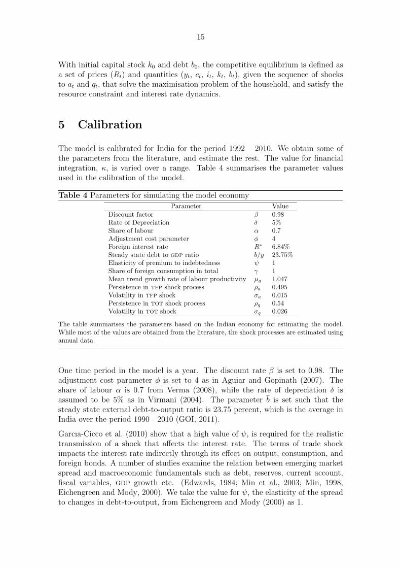
6.1 Financial openness and volatility
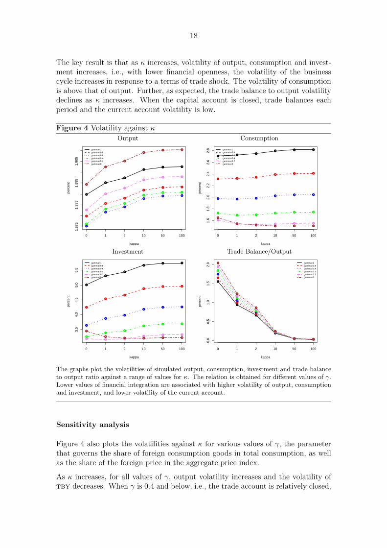
Figure 4 plots the volatilities of output, consumption, investment and trade balanceto output from the model, for a range of values of κ, where κ = 0 implies full financialintegration and κ = 100 represents financial autarky. The baseline parametrisationhas γ = 1 indicating trade openness (the solid black line).
18
The key result is that as κ increases, volatility of output, consumption and invest-ment increases, i.e., with lower financial openness, the volatility of the businesscycle increases in response to a terms of trade shock. The volatility of consumptionis above that of output. Further, as expected, the trade balance to output volatilitydeclines as κ increases. When the capital account is closed, trade balances eachperiod and the current account volatility is low.
Figure 4 Volatility against κ
Output Consumption
●
●
●
●● ●
1.87
51.
885
1.89
51.
905
kappa
perc
ent
●
●
●
●
● ●
●
●
●
●
● ●
●
●
●
●
● ●
●
●
●
●
● ●
●
●
●
●● ●
0 1 2 10 50 100
gamma=1gamma=0.8gamma=0.6gamma=0.4gamma=0.2gamma=0
●●
●
● ● ●
1.6
1.8
2.0
2.2
2.4
2.6
2.8
kappa
perc
ent
● ●●
●● ●
● ● ●● ● ●
●● ●
● ● ●
●
● ● ● ● ●
●
●● ● ● ●
0 1 2 10 50 100
gamma=1gamma=0.8gamma=0.6gamma=0.4gamma=0.2gamma=0
Investment Trade Balance/Output
●
●
●
●● ●
3.5
4.0
4.5
5.0
5.5
kappa
perc
ent
●
●
●
●● ●
●
●
●
●● ●
●
●●
●● ●
● ● ●
●● ●
●
●● ● ● ●
0 1 2 10 50 100
gamma=1gamma=0.8gamma=0.6gamma=0.4gamma=0.2gamma=0
●
●
●
●
● ●
0.0
0.5
1.0
1.5
2.0
kappa
perc
ent
●
●
●
●
● ●
●
●
●
●
● ●
●
●
●
●
● ●
●
●
●
●
● ●
●
●
●
●
● ●
0 1 2 10 50 100
gamma=1gamma=0.8gamma=0.6gamma=0.4gamma=0.2gamma=0
The graphs plot the volatilities of simulated output, consumption, investment and trade balanceto output ratio against a range of values for κ. The relation is obtained for different values of γ.Lower values of financial integration are associated with higher volatility of output, consumptionand investment, and lower volatility of the current account.
Sensitivity analysis
Figure 4 also plots the volatilities against κ for various values of γ, the parameterthat governs the share of foreign consumption goods in total consumption, as wellas the share of the foreign price in the aggregate price index.
As κ increases, for all values of γ, output volatility increases and the volatility oftby decreases. When γ is 0.4 and below, i.e., the trade account is relatively closed,
19
the volatility of consumption falls below that of output. When γ = 0, the volatilityof consumption and investment declines as κ increases.
6.2 Business cycle features of an emerging economy
We check whether the model with terms of trade shocks can explain the businesscycle features of an emerging economy. We compare the moments from the modelwith the data for an emerging economy that is characterised by limited financialopenness and higher trade openness, namely India.
India: Model and data moments
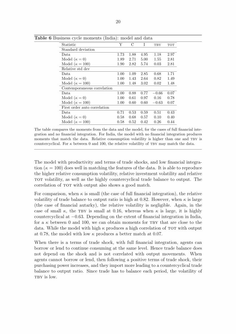
The key moments of the business cycle, i.e., volatility, relative volatility to output,contemporaneous correlation and autocorrelation are reported in the first row undereach category in Table 6. Data on output (gdp), consumption (private consumptionexpenditure), investment (gross fixed capital formation), tby or trade-balance-to-gdp (ratio of net export to gdp) and tot (ratio of cpi-iw to wpi) are loggedand detrended using the Hodrick Prescott filter to obtain the cyclical components4.The time period considered is 1992 – 2010. This is the period post reforms, whenthe economy transitioned to a more market driven system characterised by cyclicalmovements in output, consumption and investment. In this period, the business cy-cle properties of India are similar to those documented for other emerging economies(Ghate et al., 2013; Aguiar and Gopinath, 2007). Consumption and investment aremore volatile than output, while trade-balance-to-output ratio is less volatile thanoutput. Consumption and investment are procyclical, while tby is strongly coun-tercyclical. The terms of trade are more volatile than output and mildly procyclical.
The second row reports the moments from the model with full financial integration(κ = 0). The third row shows the moments for the case of high costs to financialintegration (κ = 100).
4The data are obtained from National Accounts Statistics.
20
Table 6 Business cycle moments (India): model and data
Statistic Y C I tby totStandard deviationData 1.73 1.88 4.95 1.18 2.97Model (κ = 0) 1.89 2.71 5.00 1.55 2.81Model (κ = 100) 1.90 2.82 5.74 0.03 2.81Relative std devData 1.00 1.09 2.85 0.68 1.71Model (κ = 0) 1.00 1.43 2.64 0.82 1.49Model (κ = 100) 1.00 1.48 3.02 0.02 1.48Contemporaneous correlationData 1.00 0.88 0.77 −0.66 0.07Model (κ = 0) 1.00 0.61 0.97 0.16 0.78Model (κ = 100) 1.00 0.60 0.60 −0.63 0.07First order auto correlationData 0.71 0.53 0.59 0.51 0.43Model (κ = 0) 0.58 0.68 0.57 0.10 0.40Model (κ = 100) 0.58 0.52 0.42 0.26 0.44
The table compares the moments from the data and the model, for the cases of full financial inte-gration and no financial integration. For India, the model with no financial integration producesmoments that match the data. Relative consumption volatility is higher than one and tby iscountercyclical. For κ between 0 and 100, the relative volatility of tby may match the data.
The model with productivity and terms of trade shocks, and low financial integra-tion (κ = 100) does well in matching the features of the data. It is able to reproducethe higher relative consumption volatility, relative investment volatility and relativetot volatility, as well as the highly countercyclical trade balance to output. Thecorrelation of tot with output also shows a good match.
For comparison, when κ is small (the case of full financial integration), the relativevolatility of trade balance to output ratio is high at 0.82. However, when κ is large(the case of financial autarky), the relative volatility is negligible. Again, in thecase of small κ, the tby is small at 0.16, whereas when κ is large, it is highlycountercyclical at −0.63. Depending on the extent of financial integration in India,for a κ between 0 and 100, we can obtain moments for tby that are close to thedata. While the model with high κ produces a high correlation of tot with outputat 0.78, the model with low κ produces a better match at 0.07.
When there is a terms of trade shock, with full financial integration, agents canborrow or lend to continue consuming at the same level. Hence trade balance doesnot depend on the shock and is not correlated with output movements. Whenagents cannot borrow or lend, then following a positive terms of trade shock, theirpurchasing power increases, and they import more leading to a countercyclical tradebalance to output ratio. Since trade has to balance each period, the volatility oftby is low.
21
An economy with high financial openness
We compare the results of the model to another type of emerging economy that isexposed to similar tot shocks as India, but has higher relative financial openness.Using annual data (1995 – 2010), we calculate the moments for output, consump-tion, investment and tot for Brazil.5 The standard deviation of tot is 4.39 (forIndia the standard deviation is 6.39 using this data). As seen in Table 1, the ratioof trade openness to financial openness for Brazil is 0.29.
We assume the same deep parameters hold for Brazil and compare the momentsfrom the model when κ = 0 (the case of financial integration), and the data.
Table 7 Business cycle moments (Brazil): model and data
Statistic Y C I tby totStandard deviationBrazil (1995-2010) 1.63 2.23 6.60 1.32 4.39Model (κ = 0) 1.89 2.71 5.00 1.55 2.81Relative std devBrazil 1.00 1.37 4.04 0.81 2.69Model (κ = 0) 1.00 1.43 2.64 0.82 1.49Contemporaneous correlationBrazil 1.00 0.75 0.84 −0.53 0.68Model (κ = 0) 1.00 0.61 0.97 0.16 0.78
The table compares the moments from the data and the model, for the case of full financialintegration in Brazil. The model reproduces the higher relative volatility of tby.
As seen in Table 7, the model is able to match the relative volatility of trade balanceto output ratio of 0.8. With higher financial openness, the economy is not restrictedto balance its current account, and hence its volatility is higher. The correlation oftot with output is also high as in the data. However, the data for Brazil showscountercyclical trade balance to output at −0.53, whereas the model produces apositive correlation when κ = 0. As κ increases to 100, seen in the previous table,this correlation becomes negative. For an exact parametrisation of κ between 0 and100, for the Brazilian economy, we may be able to match this moment.
7 Conclusion
We show that emerging economies vary with regard to the level of openness oftheir current and capital accounts. Our results suggest that the nature of opennessmay influence their ability to absorb external shocks. We find that in the presenceof terms of trade shocks, as financial openness increases, business cycle volatilitydecreases.
5Data on gdp, private consumption, gross fixed capital formation, exports and imports areobtained from ifs and data on net barter tot are from wdi.
22
We present a small open economy model with productivity and terms of trade shocksand calibrate it to Indian data. The model does well in matching the features of thedata by replicating the higher relative consumption volatility, the countercyclicaltrade balance and the lower relative volatility of trade balance to output.
Empirical evidence on the relation between financial integration and macroeconomicvolatility is ambiguous for emerging economies (Kose et al., 2003). Our modelpredicts that financial integration reduces business cycle volatility. But this is nottrue in general for an emerging economy. The degree of financial openness versustrade openness, and the relation to external shocks matter. Both these ideas havebeen explored to some extent in the empirical literature. One, the heterogeneityamong emerging economies due to many reasons, including structural features (Koseet al., 2011); and two, the role of shocks in determining this relation (Razin andRose, 1994). Similar to the implications of our result, von Hagen and Zhang (2006)suggest that pooling emerging economies with different levels of financial integrationmay not predict a significant relation between financial openness and volatility.
Our result has interesting policy implications. Emerging economies are subjectto external shocks that may influence their business cycle. By increasing capitalaccount openness, they can borrow and lend in international financial markets,which may help absorb shocks to the economy and stabilise the business cycle.Financial integration is, however, not without difficulties. This model, does not,for example, account for sudden stops or capital surges such as in Korinek (2011).Further, if capital flows to emerging economies are pro-cyclical as described inKaminsky et al. (2005), the net effect may be to increase, rather than reduce thevolatility of macroeconomic variables. Financial openness may expose the economyto financial shocks that may influence the business cycle as in Garcıa-Cicco et al.(2010). These aspects should be considered in further research.
In this paper, we have abstracted from the effect of the exchange rate regime onthe relation between external shocks and business cycle volatility. Flexibility inthe exchange rate regime may be another channel that could help absorb externalshocks as shown by (Broda, 2004). The role of exchange rate flexibility as well as itsinteraction with financial openness in stabilising the business cycle of an emergingeconomy that is exposed to tot shocks is another area for further research.
23
References
Abiad, A., T. Tressel, and E. Detragiache (2008). A new database of financial reforms,Volume 8. International Monetary Fund.
Aguiar, M. and G. Gopinath (2007). Emerging market business cycles: The cycle is thetrend. Journal of Political Economy 115 (1), 69–102.
Broda, C. (2004). Terms of trade and exchange rate regimes in developing countries.Journal of International Economics 63 (1), 31–58.
Buch, C., J. Dopke, and C. Pierdzioch (2005). Financial openness and business cyclevolatility. Journal of International Money and Finance 24 (5), 744–765.
Cakici, S. (2011). Financial integration and business cycles in a small open economy.Journal of International Money and Finance 30 (7), 1280–1302.
Chang, R. and A. Fernandez (2010). On the sources of aggregate fluctuations in emergingeconomies. Working Paper No. 15938, National Bureau of Economic Research.
Chinn, M. and H. Ito (2008, September). A new measure of financial openness. Journalof Comparative Policy Analysis 10 (3), 309–322.
Edwards, S. (1984). LDC foreign borrowing and default risk: An empirical investigation.American Economic Review 74 (4), 726–734.
Eichengreen, B. and A. Mody (2000). What explains changing spreads on emerging-market debt. In S. Edwards (Ed.), Capital Flows and the Emerging Economies: Theory,Evidence, and Controversies, pp. 107–136.
Evans, M. and V. Hnatkovska (2007). International financial integration and the realeconomy. IMF Staff Papers 54 (2), 220–269.
Garcıa-Cicco, J., R. Pancrazi, and M. Uribe (2010). Real business cycles in emergingcountries? American Economic Review 100 (5), 2510–31.
Ghate, C., R. Pandey, and I. Patnaik (2013). Has India emerged? Business cycle stylizedfacts from a transitioning economy. Forthcoming, Structural Change and EconomicDynamics.
GOI (2011). Status Report on India’s External Debt. External Debt Management Unit,Department of Economic Affairs, Ministry of Finance.
Kaminsky, G., C. Reinhart, and C. Vegh (2005). When it rains, it pours: procyclicalcapital flows and macroeconomic policies. In NBER Macroeconomics Annual 2004,Volume 19, pp. 11–82. MIT Press.
Korinek, A. (2011). The New Economics of Capital Controls Imposed for PrudentialReasons. IMF Economic Review (59), 523–561.
Kose, A. (2002). Explaining business cycles in small open economies: How much do worldprices matter? Journal of International Economics 56 (2), 299–328.
Kose, A., E. Prasad, and A. Taylor (2011). Thresholds in the process of internationalfinancial integration. Journal of International Money and Finance 30 (1), 147–179.
24
Kose, A., E. Prasad, and M. Terrones (2003). Financial integration and macroeconomicvolatility. IMF Working Paper.
Lane, P. and G. Milesi-Feretti (2007, November). The external wealth of nations markII: Revised and extended estimates of foreign assets and liabilities, 1970–2004. Journalof International Economics 73, 223–250.
Levchenko, A. (2004). Financial liberalization and consumption volatility in developingcountries. IMF.
Lubik, T. and W. Teo (2005). Do world shocks drive domestic business cycles? some evi-dence from structural estimation. Unpublished manuscript, Johns Hopkins University .
Mendoza, E. (1991). Real business cycles in a small open economy. The AmericanEconomic Review 81 (4), 797–818.
Mendoza, E. (1995). The terms of trade, the real exchange rate, and economic fluctuations.International Economic Review 36 (1), 101–137.
Min, H. (1998). Determinants of emerging market bond spread: Do economic fundamen-tals matter? Policy, Research Working Paper No. 1899, World Bank Publications.
Min, H., D. Lee, C. Nam, M. Park, and S. Nam (2003). Determinants of emerging-marketbond spreads: Cross-country evidence. Global Finance Journal 14 (3), 271–286.
Neumeyer, P. and F. Perri (2005). Business cycles in emerging economies: The role ofinterest rates. Journal of Monetary Economics 52 (2), 345–380.
Patnaik, I. and A. Shah (2011). Did the indian capital controls work as a tool of macroe-conomic policy? Working paper 2011-87, National Institute of Public Finance andPolicy.
Patnaik, I., A. Shah, and G. Veronese (2011). How should inflation be measured in india.Economic and Political Weekly XLVI (16).
Quinn, D. and A. Toyoda (2007). Ideology and voter preferences as determinants offinancial globalization. American Journal of Political Science 51 (2), 344–363.
Razin, A. and A. Rose (1994). Business cycle volatility and openness: An exploratorycross-section analysis. In L. Leiderman and A. Razin (Eds.), Capital Mobility: TheImpact on consumption, Investment and Growth, pp. 48 – 75. Cambridge UniversityPress.
Schindler, M. (2009). Measuring financial integration: A new data set. IMF Staff Pa-pers 56 (1), 222–238.
Uribe, M. and V. Yue (2006). Country spreads and emerging markets: Who drives whom?Journal of International Economics 69 (1), 6–36.
Verma, R. (2008). The Service Sector Revolution in India. Research Paper No. 2008/72,United Nations University.
Virmani, A. (2004). Sources of India’s Economic Growth: Trends in Total Factor Produc-tivity. ICRIER Working Paper No. 131, Indian Council for Research on InternationalEconomic Relations.
25
von Hagen, J. and H. Zhang (2006). Financial openness and macroeconomic volatility.Technical report, ZEI working paper.