Embed Size (px)
Citation preview

TSE‐612
“InvestmentPriceRigiditiesandBusinessCycles”
AlbanMoura
November 2015
INVESTMENT PRICE RIGIDITIES
AND BUSINESS CYCLES
ALBAN MOURA
Abstract. I incorporate investment price rigidity in a two-sector monetary model
of business cycles. Fit to quarterly U.S. time series, the model suggests that price
sluggishness in the investment sector is the single most empirically relevant friction
to match the data. Sticky investment prices constitutes an important propagation
mechanism to understand the sources of aggregate fluctuations, the dynamic effects of
technology shocks, and the properties of the relative price of investment goods.
JEL Codes: E3, E5.
Keywords: multisector DSGE model, investment price stickiness, relative price of in-
vestment.
First version: July 2015. This version: December 2015. Toulouse School of Economics (GREMAQ).
E-mail: [email protected]. For helpful comments, I thank T. Chaney, P. Feve, C. Hellwig,
and F. Portier. Any remaining errors are my own.1

INVESTMENT PRICE RIGIDITIES 2
1. Introduction
Price stickiness matters for macroeconomic outcomes. This form of nominal rigidity
underlies the ubiquitous New Keynesian model of monetary policy (Woodford, 2003)
and constitutes one of the building blocks of the growing literature on quantitative
dynamic stochastic general equilibrium (DSGE) models (Christiano, Eichenbaum, and
Evans, 2005; Smets and Wouters, 2007). It has proven important to understand the
general equilibrium effects of shocks to monetary or fiscal policy, as well as to technology.
Eventually, it is supported by microeconomic evidence on the behavior of individual
prices, which suggests that aggregate prices can be sticky even though micro-level prices
change frequently (Kehoe and Midrigan, 2010).
Guided by the widespread use of one-sector models, the literature has mostly focused
on price rigidity in the consumption sector. Even benchmark two-sector DSGE models,
for instance Justiniano, Primiceri, and Tambalotti (2010, 2011), feature sticky consump-
tion prices but flexible investment prices. While convenient for aggregation, ruling out
nominal frictions in the investment sector imposes strong limitations on the model’s
internal mechanisms. For instance, Basu, Fernald, and Liu (2013) demonstrate that
the propagation of technology shocks is highly sensitive to the presence of investment
price stickiness and Barsky, House, and Kimball (2007) show that this is also true of
monetary policy shocks. Additionally, there is ample empirical evidence that investment
prices are indeed sluggish. Bils and Klenow (2004) report that the monthly frequency
of price changes for durable goods, typically classified as investment in DSGE models, is
virtually the same as that for nondurable goods, close to 30 percent. Moreover, Basu,
Fernald, Fisher, and Kimball (2011) find that the pass-through of technology shocks to
prices takes several years in the investment sector, again suggestive of strong rigidities.
Eventually, price sluggishness is a well-known characteristic of the housing market (Case
and Shiller, 1989; Iacoviello, 2010).
In this context, my contribution in this paper is threefold. First, I use standard
Bayesian methods to confirm the empirical relevance of investment price rigidity within
a monetary DSGE model.1 I consider a two-sector economy, where the sectors produce
respectively consumption and investment goods. Building on the RBC literature, the
model includes real reallocation frictions in production factors through imperfect substi-
tution of hours worked and capital services across sectors. Following Barsky, House, and
Kimball (2007) and Basu, Fernald, and Liu (2013), it also incorporates sector-specific
1To my knowledge, Bouakez, Cardia, and Ruge-Murcia (2014) is the only alternative paper formally
estimating a multisector DSGE model with sector-specific pricing frictions. However, their perspective
is fundamentally different from mine as they use a much more disaggregated structure and base their
estimation on price microdata. This is not comparable to the DSGE literature I address in this paper.

INVESTMENT PRICE RIGIDITIES 3
nominal rigidities, with different frequencies of price and wage adjustments across sec-
tors. Finally, on top of the usual economy-wide shocks to preferences or monetary policy,
the model includes a rich array of sectoral disturbances affecting technology, price and
wage markups, and government purchases.
I estimate the model using quarterly U.S. time series. To sharpen identification, I
include both aggregate and sectoral variables among observables. The estimated model
captures the salient features of the data and, in particular, it correctly reproduces aggre-
gate and sectoral macro comovements. Both real reallocation frictions and sector-specific
nominal rigidities are needed to obtain a good fit, but the latter are significantly more
important. Remarkably, price stickiness in the investment sector constitutes the single
most important friction to fit the data, even though it is typically ignored by the DSGE
literature.
Second, I analyze the role of investment price rigidity in business-cycle dynamics. Re-
garding the sources of business cycles, the model confirms findings from earlier research,
for instance Justiniano, Primiceri, and Tambalotti (2011): shocks to the marginal effi-
ciency of investment (MEI) are the most important drivers of U.S. economic fluctuations.
These disturbances affect the transformation of investment goods into installed capital
and leave the productivity of investment-producing firms unchanged, thus constituting
pure investment demand shifters. My results show that their predominant role is robust
to the introduction of pricing frictions in the investment sector.
On the other hand, investment price stickiness constitutes a key mechanism to un-
derstand the dynamic effects of technology shocks. The model implies that technology
improvements are expansionary in the consumption sector and instead contractionary in
the investment sector. These patterns, consistent with Basu, Fernald, Fisher, and Kim-
ball’s (2011) growth-accounting results, have not been previously documented within
the empirical DSGE literature. The underlying economic intuition, developed in Barsky,
House, and Kimball (2007) and Basu, Fernald, and Liu (2013), is straightforward. With
sluggish prices, an improvement in investment technology makes current investment ex-
pensive relative to the future since firms adjust only gradually their prices. Investment
demand being highly elastic, current demand falls and triggers a generalized recession.
Symmetrically, an improvement in consumption technology makes current investment
relatively cheaper and generates an expansion.
Third, I examine the link between relative technology shocks and the relative price of
investment goods. While much of the DSGE literature imposes flexible investment prices,
extended nominal rigidities break the usual identity between relative technology and the
relative price. Notably, only one-fifth of the cyclical variance of the relative price of
investment is due to technology shocks in the estimated model, while the contribution of

INVESTMENT PRICE RIGIDITIES 4
markup shocks exceeds 50 percent. This result calls into question the validity of the usual
empirical approach imposing a period-by-period equality between relative technology in
the investment and consumption sectors and the relative price of investment.
The paper is organized as follows: Section 2 sets up the DSGE model, while Section
3 describes the estimation procedure and the data. Section 4 reports estimation results,
including a discussion of the model fit. Section 5 examines the implications of investment
price stickiness for the sources of business cycles, the effects of technology and monetary
shocks, and the properties of the relative price of investment. Eventually, Section 6
concludes.
2. A Two-Sector DSGE Model
The model builds on Basu, Fernald, and Liu (2013), who extend the medium-scale
sticky-price economies from Smets and Wouters (2007) and Justiniano, Primiceri, and
Tambalotti (2010, 2011) to an explicit two-sector structure. I add to their framework
frictions affecting the sectoral allocation of production factors. The economy is populated
by seven classes of agents: a final retail sector producing homogeneous consumption and
investment goods, two intermediate sectors specializing in producing inputs for the con-
sumption and investment retailers, households, competitive labor packers, monopolistic
labor unions, a central bank, and a government. Their decisions are described in turn.
2.1. Final retail sector. There are two competitive retailers, one for each sector. They
purchase a continuum of differentiated sector-specific intermediate inputs and produce
the final consumption and investment goods in quantities Y ct and Y i
t according to
Y ct =
(∫ 1
0
Y ct (j)
11+ηct dj
)1+ηct
, Y it =
(∫ 1
0
Y it (j)
1
1+ηit dj
)1+ηit
.
The elasticities ηct and ηit correspond to sector-specific price markup shocks and evolve
according to
ln(1 + ηct ) = (1− ρηc) ln(1 + ηc) + ρηc ln(1 + ηct−1) + εηct − θcεηct−1,
ln(1 + ηit) = (1− ρηi) ln(1 + ηi) + ρηi ln(1 + ηit−1) + εηit − θiεηit−1,
with εηct ∼ iidN(0, σ2ηc) and εηit ∼ iidN(0, σ2
ηi). Standard manipulations yield the expres-
sions of the aggregate consumption and investment prices:
P ct =
(∫ 1
0
P ct (j)
− 1ηct dj
)−ηct, P i
t =
(∫ 1
0
P it (j)
− 1
ηit dj
)−ηit.
INVESTMENT PRICE RIGIDITIES 5
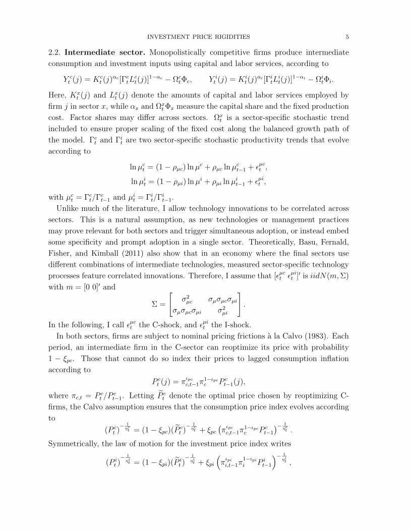
2.2. Intermediate sector. Monopolistically competitive firms produce intermediate
consumption and investment inputs using capital and labor services, according to
Y ct (j) = Kc
t (j)αc [ΓctL
ct(j)]
1−αc − ΩctΦc, Y i
t (j) = Kit(j)
αi [ΓitLit(j)]
1−αi − ΩitΦi.
Here, Kxt (j) and Lxt (j) denote the amounts of capital and labor services employed by
firm j in sector x, while αx and Ωxt Φx measure the capital share and the fixed production
cost. Factor shares may differ across sectors. Ωxt is a sector-specific stochastic trend
included to ensure proper scaling of the fixed cost along the balanced growth path of
the model. Γct and Γit are two sector-specific stochastic productivity trends that evolve
according to
lnµct = (1− ρµc) lnµc + ρµc lnµct−1 + εµct ,
lnµit = (1− ρµi) lnµi + ρµi lnµit−1 + εµit ,
with µct = Γct/Γct−1 and µit = Γit/Γ
it−1.
Unlike much of the literature, I allow technology innovations to be correlated across
sectors. This is a natural assumption, as new technologies or management practices
may prove relevant for both sectors and trigger simultaneous adoption, or instead embed
some specificity and prompt adoption in a single sector. Theoretically, Basu, Fernald,
Fisher, and Kimball (2011) also show that in an economy where the final sectors use
different combinations of intermediate technologies, measured sector-specific technology
processes feature correlated innovations. Therefore, I assume that [εµct εµit ]′ is iidN(m,Σ)
with m = [0 0]′ and
Σ =
[σ2µc σµσµcσµi
σµσµcσµi σ2µi
].
In the following, I call εµct the C-shock, and εµit the I-shock.
In both sectors, firms are subject to nominal pricing frictions a la Calvo (1983). Each
period, an intermediate firm in the C-sector can reoptimize its price with probability
1 − ξpc. Those that cannot do so index their prices to lagged consumption inflation
according to
P ct (j) = π
ιpcc,t−1π
1−ιpcc P c
t−1(j),
where πc,t = P ct /P
ct−1. Letting P c
t denote the optimal price chosen by reoptimizing C-
firms, the Calvo assumption ensures that the consumption price index evolves according
to
(P ct )− 1ηct = (1− ξpc)(P c
t )− 1ηct + ξpc
(πιpcc,t−1π
1−ιpcc P c
t−1)− 1
ηct .
Symmetrically, the law of motion for the investment price index writes
(P it )− 1
ηit = (1− ξpi)(P it )− 1
ηit + ξpi
(πιpii,t−1π
1−ιpii P i
t−1
)− 1
ηit ,

INVESTMENT PRICE RIGIDITIES 6
where P it denote the optimal price for a reoptimizing I-firm, ξpi and ιpi are the Calvo
and indexation parameters in the I-sector, and πi,t = P it /P
it−1.
Consolidating the last two equations yields an expression for the relative price of
investment goods, RPIt = P it /P
ct . Absent Calvo frictions, the nominal price in each
sector is equal to the product of the exogenous sector-specific markup with the nominal
marginal cost. In that case, RPIt takes the simple form
P it
P ct
∝ 1 + ηit1 + ηct
(Γct)1−αc
(Γit)1−αi
(W it )
1−αi(Rkit )αi
(W ct )1−αc(Rkc
t )αc,
where W xt and Rx
t denote the nominal wage and rental rate of capital for firms in sector x.
This expression shows that fluctuations in the relative price of investment originate from
three different sources: (i) shifts in relative markups across sectors, (ii) shifts in relative
technology across sectors, and (iii) shifts in the unit production cost across sectors. By
assumption, points (i) and (ii) relate to exogenous factors. On the other hand, point (iii)
implies that all shocks hitting the economy will be endogenously passed to the relative
price in presence of limited factor mobility or differences in factor shares. If nominal
rigidities pop in, the same logic applies but the pass-through of non-markup shocks to
the relative price of investment may be considerably slowed down.
The implication that all shocks affect the equilibrium path of the relative price of
investment is in sharp contrast with the assumption of a direct mapping between RPItand relative technology across sectors typically embedded in estimated DSGE models.
Within the economy at hand, such a tight link would arise as a knife-edge case in a
restricted specification with price flexibility, perfectly competitive good markets, full
factor mobility, and identical factor shares across sectors. I show in the estimation
exercise below that such restrictions are strongly rejected by U.S. data.
2.3. Households. The economy is populated by a measure one of households. The
representative household’s lifetime utility function writes
E0
∞∑t=0
βtζt
[(Ct − hCt−1)
1−σ
1− σexp
(σ − 1
1 + κ
[(Lct)
1+ω + (Lit)1+ω] 1+κ
1+ω
)],
where Ct, Lct , and Lit respectively denote individual consumption and hours worked in
the C- and I-sectors, Ct =∫ 1
0Ct(l)dl is the average level of consumption in the economy,
β ∈ (0, 1) is the discount factor, σ is the risk-aversion coefficient, and h ∈ (0, 1) measures
external habit formation. As in Horvath (2000), the specification of the disutility of
working implies imperfect labor mobility across sectors when ω > 0, allowing for sectoral
heterogeneity in wages and hours worked. κ ≥ 0 measures the aggregate elasticity of
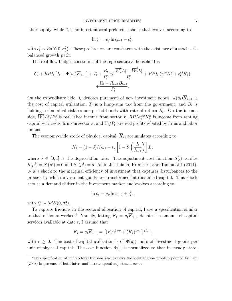
INVESTMENT PRICE RIGIDITIES 7
labor supply, while ζt is an intertemporal preference shock that evolves according to
ln ζt = ρζ ln ζt−1 + εζt ,
with εζt ∼ iidN(0, σ2ζ ). These preferences are consistent with the existence of a stochastic
balanced growth path.
The real flow budget constraint of the representative household is
Ct +RPIt[It + Ψ(ut)Kt−1
]+ Tt +
Bt
P ct
≤ Wc
tLct +W
i
tLit
P ct
+RPIt(rkct K
ct + rkit K
it
)+
Πt +Rt−1Bt−1
P ct
.
On the expenditure side, It denotes purchases of new investment goods, Ψ(ut)Kt−1 is
the cost of capital utilization, Tt is a lump-sum tax from the government, and Bt is
holdings of nominal riskless one-period bonds with rate of return Rt. On the income
side, Wx
tLxt /P
ct is real labor income from sector x, RPItr
kxt K
xt is income from renting
capital services to firms in sector x, and Πt/Pct are real profits rebated by firms and labor
unions.
The economy-wide stock of physical capital, Kt, accumulates according to
Kt = (1− δ)Kt−1 + υt
[1− S
(ItIt−1
)]It,
where δ ∈ [0, 1] is the depreciation rate. The adjustment cost function S(.) verifies
S(µi) = S ′(µi) = 0 and S ′′(µi) = s. As in Justiniano, Primiceri, and Tambalotti (2011),
υt is a shock to the marginal efficiency of investment that captures disturbances to the
process by which investment goods are transformed into installed capital. This shock
acts as a demand shifter in the investment market and evolves according to
ln υt = ρυ ln υt−1 + ευt ,
with ευt ∼ iidN(0, σ2υ).
To capture frictions in the sectoral allocation of capital, I use a specification similar
to that of hours worked.2 Namely, letting Kt = utKt−1 denote the amount of capital
services available at date t, I assume that
Kt = utKt−1 =[(Kc
t )1+ν + (Ki
t)1+ν] 1
1+ν ,
with ν ≥ 0. The cost of capital utilization is of Ψ(ut) units of investment goods per
unit of physical capital. The cost function Ψ(.) is normalized so that in steady state,
2This specification of intersectoral frictions also eschews the identification problem pointed by Kim
(2003) in presence of both inter- and intratemporal adjustment costs.

INVESTMENT PRICE RIGIDITIES 8
u = 1 and Ψ(1) = 0. As usual, I parametrize the function Ψ by ψ ∈ (0, 1) such that
Ψ′′(1)/Ψ′(1) = ψ/(1− ψ).
2.4. Labor market. Households supply hours worked to sector-specific unions, which
differentiate labor services and set nominal wages subject to Calvo frictions. Competitive
labor packers purchase those differentiated services and produce the final labor input
usable by firms.
2.4.1. Labor packers. There are two competitive labor packers in the economy, one for
each sector. They purchase a continuum of differentiated sector-specific labor services
and produce usable labor inputs according to
Lct =
(∫ 1
0
Lct(u)1
1+ηwct du
)1+ηwct
, Lit =
(∫ 1
0
Lit(u)1
1+ηwit du
)1+ηwit
.
The two wage markup shocks ηwct and ηwit evolve according to
ln(1 + ηwct ) = (1− ρηwc) ln(1 + ηwc) + ρηwc ln(1 + ηwct−1) + εηwct − θwcεηwct−1 ,
ln(1 + ηwit ) = (1− ρηwi) ln(1 + ηwi) + ρηwi ln(1 + ηwit−1) + εηwit − θwiεηwit−1,
with εηwct ∼ iidN(0, σ2ηwc) and εηwit ∼ iidN(0, σ2
ηwi).
2.4.2. Labor unions. In each sector, labor unions intermediate between households and
the labor packer by differentiating homogeneous hours worked and setting nominal wages.
The probability that a particular union in the C-sector can reset its nominal wage at
period t is constant and equal to 1 − ξwc, and nominal wages that are not reoptimized
are partially indexed according to
W ct (u) = (πc,t−1µ
wct−1)
ιwc(πcµ)1−ιwcW ct−1(u),
where µwct is the equilibrium growth rate in the real sectoral wage W ct /P
ct , with steady-
state level µ = (µc)1−αc(µi)αc . Letting W ct denote the optimal wage chosen by reop-
timizing C-unions, the law of motion of the aggregate wage index in the C-sector is
then
(W ct )− 1ηwct = (1− ξwc)(W c
t )− 1ηwct + ξwc
[(πc,t−1µ
wct−1)
ιwc(πcµ)1−ιwcW ct−1]− 1
ηwct .
Similar computations deliver the wage equation for the I-sector:
(W it )− 1
ηwit = (1− ξwi)(W it )− 1
ηwit + ξwi[(πc,t−1µ
wit−1)
ιwi(πcµ)1−ιwiW it−1]− 1
ηwit ,
where W it denotes the optimal wage for a reoptimizing I-union and ξwi and ιwi are the
Calvo and indexation parameters in the I-sector.

INVESTMENT PRICE RIGIDITIES 9
2.5. Central bank. The monetary authority sets the nominal interest rate according
to a Taylor-like rule:
Rt
R=
(Rt−1
R
)ρr [(πc,tπc
)φπ ( Xt
µXt−1
)φx]1−ρrγmt ,
where Xt is real GDP in consumption units, defined below.3 The policy rule is shifted by
a disturbance γmt , capturing both persistent movements in the central bank’s inflation
target and discretionary monetary shocks. It evolves according to
ln γmt = ρm ln γmt−1 + εmt ,
with εmt ∼ iidN(0, σ2m).
2.6. Government. Fiscal policy is Ricardian. The government purchases exogenous
amounts of consumption and investment goods, respectively denoted Gct and Gi
t, whose
final use is not specified. In particular, I do not allow for a productive feedback from the
unmodeled stock of public capital. Letting gct = Gct/Ω
ct and git = Gi
t/Ωit denote detrended
expenditures, I assume that
ln gct = (1− ρgc) ln gc + ρgc ln gct−1 + εgct ,
ln git = (1− ρgi) ln gi + ρgi ln git−1 + εgit ,
with εgct ∼ iidN(0, σ2gc) and εgit ∼ iidN(0, σ2
gi). Lump-sum taxes Tt adjust to balance the
government budget constraint at each date:
Tt = Gct +RPItG
it.
2.7. Market clearing. Market clearing requires that Bt = 0 in the bond market, that
Ct +Gct = Y c
t ,
It +Git + Ψ(ut)Kt−1 = Y i
t
in the consumption and investment good markets, and that∫ 1
0
Kct (j)dj = Kc
t ,
∫ 1
0
Kit(j)dj = Ki
t ,∫ 1
0
Lct(j)dj = Lct ,
∫ 1
0
Lit(j)dj = Lit
3In theory, the policy rule could allow for different responses to C-inflation, I-inflation, growth in the
C-sector, and growth in the I-sector. From an empirical perspective however, this richer policy rule only
marginally improves the fit and leaves the main results unchanged. I have thus opted for the simplest
specification here.
INVESTMENT PRICE RIGIDITIES 10
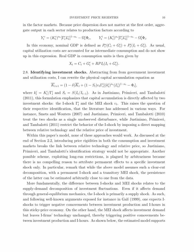
in the factor markets. Because price dispersion does not matter at the first order, aggre-
gate output in each sector relates to production factors according to
Y ct = (Kc
t )αc [ΓctL
ct ]1−αc − Ωc
tΦc, Y it = (Ki
t)αi [ΓitL
it]1−αi − Ωi
tΦi.
In this economy, nominal GDP is defined as P ct (Ct + Gc
t) + P it (It + Gi
t). As usual,
capital utilization costs are accounted for as intermediate consumption and do not show
up in this expression. Real GDP in consumption units is then given by
Xt = Ct +Gct +RPIt(It +Gi
t).
2.8. Identifying investment shocks. Abstracting from from government investment
and utilization costs, I can rewrite the physical capital accumulation equation as
Kt+1 = (1− δ)Kt + (1− St)υtΓit[(kit)αi(Lit)1−αi − Φi],
where kit = Kit/Γ
it and St = S(It/It−1). As in Justiniano, Primiceri, and Tambalotti
(2011), this formulation emphasizes that capital accumulation is directly affected by two
investment shocks: the I-shock Γit and the MEI shock υt. This raises the question of
their respective identification, that the literature has addressed in various ways. For
instance, Smets and Wouters (2007) and Justiniano, Primiceri, and Tambalotti (2010)
treat the two shocks as a single unobserved disturbance, while Justiniano, Primiceri,
and Tambalotti (2011) restrict the behavior of the I-shock by imposing a direct mapping
between relative technology and the relative price of investment.
Within this paper’s model, none of these approaches would work. As discussed at the
end of Section 2.2, introducing price rigidities in both the consumption and investment
markets breaks the link between relative technology and relative price, so Justiniano,
Primiceri, and Tambalotti’s identification strategy would not be appropriate. Another
possible scheme, exploiting long-run restrictions, is plagued by arbitrariness because
there is no compelling reason to attribute permanent effects to a specific investment
shock only. In particular, remark that while the above model assumes such a clear-cut
decomposition, with a permanent I-shock and a transitory MEI shock, the persistence
of the latter can be estimated arbitrarily close to one from the data.
More fundamentally, the difference between I-shocks and MEI shocks relates to the
supply-demand decomposition of investment fluctuations. Even if it affects demand
through general-equilibrium mechanics, the I-shock is primarily a supply shock. As such,
and following well-known arguments exposed for instance in Galı (1999), one expects I-
shocks to trigger negative comovements between investment production and I-hours in
this sticky-price economy. On the other hand, the MEI shock affects investment demand
but leaves I-firms’ technology unchanged, thereby triggering positive comovements be-
tween investment production and I-hours. As shown below, the estimated model supports

INVESTMENT PRICE RIGIDITIES 11
these intuitions, so the I- and MEI shocks are effectively identified by the different con-
ditional comovements they imply. Practically, inclusion of sectoral hours series among
observables will be key to separate out the two investment shocks during estimation.
3. Bayesian Inference
I solve the model with standard linearization techniques and use Bayesian methods
to estimate its parameters. This section discusses the data used to build the likelihood
function, the calibration of some parameters, and the specification of prior distributions
for the remaining ones.
3.1. Data. I estimate the model using eleven observables: real private consumption
growth, real private investment growth, real public consumption growth, real public in-
vestment growth, hours worked in the C-sector, hours worked in the I-sector, real wage
growth in the C-sector, real wage growth in the I-sector, inflation in the C-sector, the
relative price of investment growth rate, and a nominal interest rate. I define private
consumption as personal consumption expenditures on nondurable goods and services,
while private investment includes both expenditures on durable goods and fixed invest-
ment. I use standard chain aggregation methods to construct the relevant quantity and
price series. All quantities are expressed in per-capita terms. Appendix A provides data
sources and describes the linkage to observables.
My selection of observables differs from that typically used in the DSGE literature
in that I include substantial information about the sectoral structure of the economy.
Two objectives underlie this choice. First, sectoral observables provide a useful source
of identification for sectoral shocks and frictions. For instance, I argued in Section 2.8
that observations on I-hours were needed to separate out the two investment shocks.
Likewise, consolidating the representative consumer’s two first-order conditions for labor
supply yields
Wc
t
Wi
t
=
(LctLit
)ω,
an equation that shows it would be difficult to identify ω, the parameter capturing real-
location frictions in labor, without sectoral data on hours and wages.4 Second, matching
sectoral variables helps pushing the model toward capturing both aggregate and sectoral
4The equilibrium allocation of capital services is characterized by rkct /rkit = (Kc
t /Kit)ν . Given the
absence of data on the return to capital or the sectoral allocation of capital, identification of ν appears
somewhat more fragile.

INVESTMENT PRICE RIGIDITIES 12
comovements. Eventually, there are as many structural shocks in the model economy as
observables used in estimation.5
I demean all series prior to estimation. This procedure ensures that potential discrep-
ancies between the model’s implied balanced growth path and the data will not distort
inference at the business-cycle frequencies of interest. However, the approach also im-
plies that steady-state information will not be used for identification. The calibration
of specific parameters reflect this choice. Additionally, I remove independent quadratic
trends from the two hours series. This is required by hours worked displaying differ-
ent long-run behavior in the two sectors, with C-hours rising significantly more than
I-hours over the sample. This detrending procedure also ensures that estimation focuses
on business-cycle comovements rather than on low-frequency patterns the model is not
designed to capture.
Eventually, the estimation sample runs from 1965Q1 to 2008Q3, which is the first
quarter in which the nominal interest rate hit the zero lower bound in the U.S. economy.
3.2. Calibrated parameters. I keep thirteen model parameters fixed during estima-
tion: the subjective discount factor β; the steady-state depreciation rate δ; the four
steady-state markup parameters ηc, ηi, ηwc, and ηwi; steady-state inflation in the C-
sector πc; the steady-state growth rates in sector-specific technologies µc and µi; the
factor shares αc and αi; and the two steady-state government spending ratios Gc/Y c
and Gi/Y i. These parameters are difficult to identify without steady-state information
as they have little effect on model dynamics.
Table 1 reports the chosen values. Consistent with the estimates reported in Smets and
Wouters (2007) and Justiniano, Primiceri, and Tambalotti (2010, 2011), I set β = 0.998.
Together with the calibrated values for πc, µc, and µi and with the point estimate for the
risk aversion coefficient σ, this choice implies a steady-state annual nominal interest rate
of 7.7 percent, somewhat above the sample average of 6.4 percent. I fix the depreciation
rate of capital δ at 0.025, a standard choice for quarterly models, and assume 10 percent
markups in both good and labor markets.
I calibrate πc, µc, and µi by matching the sample averages for inflation in the C-sector,
growth in private consumption, and growth in private investment. In particular, there
is faster technological progress in the I-sector relative to the C-sector, as µi > µc. The
implied steady-state gross inflation rate in the I-sector is 1.007, in line with its sample
5Some authors (Sullivan, 1997; Iacoviello and Neri, 2010) argue that the BLS series for sectoral
hours and wages suffer from measurement error, especially regarding long-run trends. The demeaning
procedure described below is a way to cope with this issue. Additionally, I have tried estimating the
model allowing for independent measurement errors on observables. However, in that case the estimated
model missed the positive intersectoral comovement of hours worked.

INVESTMENT PRICE RIGIDITIES 13
Table 1. Calibrated parameters.
Parameter Value Description
β 0.998 Subjective discount factor
δ 0.025 Steady-state depreciation rate
ηc, ηi, ηwc, ηwi 0.10 Steady-state net good- and labor-market markups
πc 1.011 Steady-state gross C-inflation
µc 1.003 Steady-state gross growth rate in C-technology
µi 1.008 Steady-state gross growth rate in I-technology
αc 0.35 Capital share in the C-sector
αi 0.30 Capital share in the I-sector
Gc/Y c 0.23 Steady-state share of public consumption
Gi/Y i 0.15 Steady-state share of public investment
counterpart. Thus, the model matches the steady-state gross growth rate in the relative
price of investment as well. I use Basu, Fernald, Fisher, and Kimball’s (2011) growth-
accounting estimates of sectoral capital shares to fix αc and αi. They report final-use
capital shares equal to 0.36 for consumption-producing firms and to 0.35 for government
consumption, so I set αc = 0.35, as well as capital shares ranging from 0.26 to 0.31
for investment-producing firms, which I aggregate into αi = 0.30. Eventually, I fix the
steady-state ratios of public to private consumption and public to private investment by
matching their sample averages.
3.3. Prior distributions. I estimate all remaining parameters. The first columns in
Tables 2 and 3 display the chosen prior distributions. Most are in line with the previous
DSGE literature.
Starting the representative household’s preferences, the risk aversion coefficient σ has a
prior mean of 1.5, the habit parameter h is centered around 0.6, and the inverse elasticity
of labor supply κ fluctuates around 2. The prior distribution for ω, the parameter
capturing the elasticity of substitution across hours in the two sectors, has a mean of 2,
somewhat above the value of one estimated by Horvath (2000) in a more disaggregated
model. Indeed, a prior predictive analysis conducted before estimation emphasized the
role of large ω values in generating sectoral comovements. Yet, to let the data speak
as much as possible, I adopt a fairly diffuse gamma prior with a standard deviation of
0.75. I use an identical prior for ν, the parameter quantifying sectoral frictions in capital
reallocation.
Prior distributions for other friction parameters are quite standard. In particular, I
choose beta distributions centered at 0.65 for the four Calvo coefficients. Regarding
INVESTMENT PRICE RIGIDITIES 14
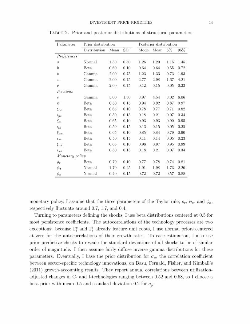
Table 2. Prior and posterior distributions of structural parameters.
Parameter Prior distribution Posterior distribution
Distribution Mean SD Mode Mean 5% 95%
Preferences
σ Normal 1.50 0.30 1.26 1.29 1.15 1.45
h Beta 0.60 0.10 0.64 0.64 0.55 0.72
κ Gamma 2.00 0.75 1.23 1.33 0.73 1.93
ω Gamma 2.00 0.75 2.77 2.98 1.67 4.21
ν Gamma 2.00 0.75 0.12 0.15 0.05 0.23
Frictions
s Gamma 5.00 1.50 3.97 4.54 3.02 6.06
ψ Beta 0.50 0.15 0.94 0.92 0.87 0.97
ξpc Beta 0.65 0.10 0.78 0.77 0.71 0.82
ιpc Beta 0.50 0.15 0.18 0.21 0.07 0.34
ξpi Beta 0.65 0.10 0.93 0.93 0.90 0.95
ιpi Beta 0.50 0.15 0.13 0.15 0.05 0.25
ξwc Beta 0.65 0.10 0.85 0.84 0.79 0.90
ιwc Beta 0.50 0.15 0.11 0.14 0.05 0.23
ξwi Beta 0.65 0.10 0.98 0.97 0.95 0.99
ιwi Beta 0.50 0.15 0.18 0.21 0.07 0.34
Monetary policy
ρr Beta 0.70 0.10 0.77 0.78 0.74 0.81
φπ Normal 1.70 0.25 1.91 1.98 1.73 2.20
φx Normal 0.40 0.15 0.72 0.72 0.57 0.88
monetary policy, I assume that the three parameters of the Taylor rule, ρr, φπ, and φx,
respectively fluctuate around 0.7, 1.7, and 0.4.
Turning to parameters defining the shocks, I use beta distributions centered at 0.5 for
most persistence coefficients. The autocorrelations of the technology processes are two
exceptions: because Γct and Γit already feature unit roots, I use normal priors centered
at zero for the autocorrelations of their growth rates. To ease estimation, I also use
prior predictive checks to rescale the standard deviations of all shocks to be of similar
order of magnitude. I then assume fairly diffuse inverse gamma distributions for these
parameters. Eventually, I base the prior distribution for σµ, the correlation coefficient
between sector-specific technology innovations, on Basu, Fernald, Fisher, and Kimball’s
(2011) growth-accounting results. They report annual correlations between utilization-
adjusted changes in C- and I-technologies ranging between 0.52 and 0.58, so I choose a
beta prior with mean 0.5 and standard deviation 0.2 for σµ.
INVESTMENT PRICE RIGIDITIES 15
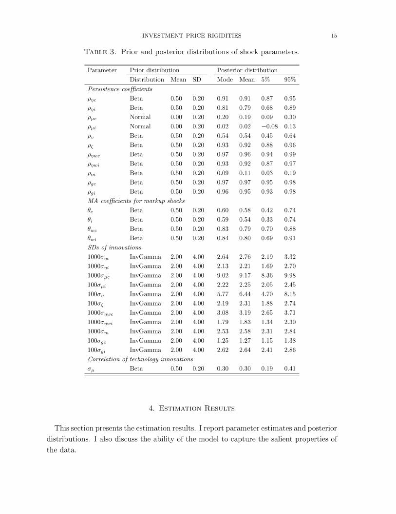
Table 3. Prior and posterior distributions of shock parameters.
Parameter Prior distribution Posterior distribution
Distribution Mean SD Mode Mean 5% 95%
Persistence coefficients
ρηc Beta 0.50 0.20 0.91 0.91 0.87 0.95
ρηi Beta 0.50 0.20 0.81 0.79 0.68 0.89
ρµc Normal 0.00 0.20 0.20 0.19 0.09 0.30
ρµi Normal 0.00 0.20 0.02 0.02 −0.08 0.13
ρυ Beta 0.50 0.20 0.54 0.54 0.45 0.64
ρζ Beta 0.50 0.20 0.93 0.92 0.88 0.96
ρηwc Beta 0.50 0.20 0.97 0.96 0.94 0.99
ρηwi Beta 0.50 0.20 0.93 0.92 0.87 0.97
ρm Beta 0.50 0.20 0.09 0.11 0.03 0.19
ρgc Beta 0.50 0.20 0.97 0.97 0.95 0.98
ρgi Beta 0.50 0.20 0.96 0.95 0.93 0.98
MA coefficients for markup shocks
θc Beta 0.50 0.20 0.60 0.58 0.42 0.74
θi Beta 0.50 0.20 0.59 0.54 0.33 0.74
θwc Beta 0.50 0.20 0.83 0.79 0.70 0.88
θwi Beta 0.50 0.20 0.84 0.80 0.69 0.91
SDs of innovations
1000σηc InvGamma 2.00 4.00 2.64 2.76 2.19 3.32
1000σηi InvGamma 2.00 4.00 2.13 2.21 1.69 2.70
1000σµc InvGamma 2.00 4.00 9.02 9.17 8.36 9.98
100σµi InvGamma 2.00 4.00 2.22 2.25 2.05 2.45
100συ InvGamma 2.00 4.00 5.77 6.44 4.70 8.15
100σζ InvGamma 2.00 4.00 2.19 2.31 1.88 2.74
1000σηwc InvGamma 2.00 4.00 3.08 3.19 2.65 3.71
1000σηwi InvGamma 2.00 4.00 1.79 1.83 1.34 2.30
1000σm InvGamma 2.00 4.00 2.53 2.58 2.31 2.84
100σgc InvGamma 2.00 4.00 1.25 1.27 1.15 1.38
100σgi InvGamma 2.00 4.00 2.62 2.64 2.41 2.86
Correlation of technology innovations
σµ Beta 0.50 0.20 0.30 0.30 0.19 0.41
4. Estimation Results
This section presents the estimation results. I report parameter estimates and posterior
distributions. I also discuss the ability of the model to capture the salient properties of
the data.
INVESTMENT PRICE RIGIDITIES 16
4.1. Posterior distributions. The last columns in Tables 2 and 3 report the poste-
rior modes, means, and 90% probability intervals for the estimated parameters.6 All
parameters seem well identified from the data.
On the preference side, the point estimate of the risk aversion coefficient is equal to
1.26, above the value of one that would correspond to a logarithmic specification. The
representative household also displays a moderate degree of consumption habits, with
a point estimate of h close to its prior mean at 0.64. The estimated Frisch elasticity
of labor supply is close to 0.8, in the range of the microestimates reviewed in Rıos-
Rull, Schorfheide, Fuentes-Albero, Kryshko, and Santaeulalia-Llopis (2012). The point
estimate of ω is equal to 2.77, well above its prior mean. This is suggestive that the
model needs large labor adjustment costs to fit the data. On the other hand, reallocation
frictions in capital services seem unimportant, as the estimated value of ν is close to zero.
The data are strongly informative about both ω and ν, whose posterior distributions are
much tighter than the priors.
Turning to the Calvo coefficients, prices are reoptimized on average once every four
quarters in C-sector, and once every fourteen quarters in the I-sector. Although the
estimate of ξpi may appear implausibly high, remark that all prices change every period
in the model due to indexation. Thus, the low frequency of price optimization does
not translate into extreme observed price sluggishness. Also, the model abstracts from
strategic complementarities in price setting, which offer a mechanical way to lower esti-
mates of Calvo coefficients in linearized DSGE models (Eichenbaum and Fisher, 2007).
Overall, it is interesting that the data point toward higher price rigidities in the I-sector
since the DSGE literature usually assumes that ξpi = 0. Turning to wages, there is
also more rigidity in the I-sector than in the C-sector, so the usual assumption of an
aggregate labor market again hides substantial sectoral heterogeneity. Eventually, all
estimated indexation coefficients are quite low.
The estimated Taylor rule is consistent with a large empirical literature, as the central
bank reacts strongly to both C-inflation and output growth. There is some interest rate
smoothing and it is interesting to note that, given the estimated policy rule, the model
does not need a persistent monetary policy disturbance. Other forcing processes, for
instance the four markup shocks, the preference shock, and the two government spend-
ing shocks, display strong autocorrelations. Finally, the estimated correlation between
quarterly sectoral technology disturbances is equal to 0.30, only about half the value
reported by Basu, Fernald, Fisher, and Kimball (2011). While differences in datasets
6I use the random-walk Metropolis-Hastings algorithm with a single chain to construct the posterior
distribution, keeping 500, 000 draws after a burn-in period of 1, 000, 000 draws. I set the step size to
ensure an acceptance rate close to 0.32 and use standard tests to confirm convergence.
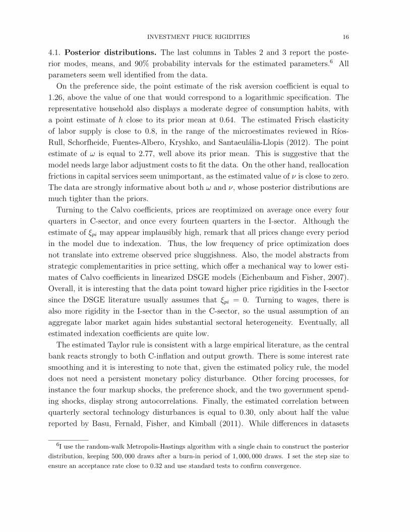
INVESTMENT PRICE RIGIDITIES 17
Figure 1. Cross-correlations at +/- 10 periods: Model vs. data.
Notes. Solid red lines represent model-based cross-correlograms, evaluated at the posterior mode, while
shaded bands represent 90% GMM confidence intervals centered around the empirical correlations, which
are not themselves displayed.
and identification strategies explain this discrepancy, I show below that the dynamic
responses of the main macro aggregates to the sectoral technology shocks estimated by
the Bayesian DSGE approach share important properties with those identified by Basu,
Fernald, Fisher, and Kimball.
4.2. Model fit. To assess the ability of the model to fit the data, Figure 1 compares
the theoretical and empirical cross-correlation functions for observables.7 Solid red lines
represent model-based moments computed at the posterior mode, while shaded bands
represent 90% GMM confidence intervals centered around the empirical correlations.
7To increase readability, I omit the two government spending series from the Figure. Their cross-
correlations functions with other variables are essentially zeros at all leads and lags, a fact correctly
captured by the model.

INVESTMENT PRICE RIGIDITIES 18
Recall that a likelihood-based estimator tries to match the entire autocovariance func-
tion of the data. It is therefore not surprising that the estimated model cannot simul-
taneously fit all moments. The general picture is, however, satisfactory and suggests
that the model captures salient properties of the U.S. economy. Plots on the diagonal
show that the own correlation structures of most variables are accurately reproduced.
The biggest discrepancies between the data and the model are the overestimated per-
sistence of I-hours and the underestimated persistence of C-inflation. All other model
autocorrelations fall within the empirical confidence bands.
In terms of macro comovements, the correlation patterns between consumption and
investment on the one hand, and C-hours and I-hours on the other, are matched well.
Notably, the growth rates of consumption and investment are positively correlated, as are
equilibrium hours in the two sectors. The only disparity relates to investment growth:
while it leads consumption growth by one quarter in the model, it does not in the
data. Also, in each sector, the dynamic correlations between physical output and labor
input are reproduced well. The model thus does a good job at accounting for business-
cycle comovements at the sectoral level. In the aggregate, the main theoretical cross-
correlations between quantities and prices lie within their empirical confidence bands.
Eventually, the model accounts well for the empirical properties of the relative price of
investment goods.
5. Macroeconomic Effects of Investment Price Stickiness
This section demonstrates the importance of investment price stickiness for business-
cycle analysis. First, I show that nominal rigidity in the investment sector is the single
most important friction in terms of fitting the data, suggesting its constitutes a powerful
propagation mechanism. I confirm this idea by studying how the introduction of invest-
ment price sluggishness affects inference about the sources of macro fluctuations and the
effects of structural economic shocks in the model. Eventually, I examine the drivers of
the relative price of investment in presence of extended nominal rigidities and conclude
against the common view that supply shocks predominate.
5.1. The empirical role of investment price rigidity. I start by assessing formally
the empirical role of investment price stickiness in terms of fitting the data. Indeed, the
model includes many different frictions and one may be worried that rigid investment
prices are not important to capture the dynamics of U.S. time series. To show that they
do matter, I reestimate the model shutting off once at a time specific channels and use
Bayes factor to evaluate the relative fit of the restricted specifications. This is a stringent
way of checking the relevance of individual frictions: since it allows other parameters to

INVESTMENT PRICE RIGIDITIES 19
Table 4. Model fit comparisons.
Model specification RestrictionLog-marginal Bayes factor relative
data density to baseline
Baseline — 6, 788 1.0
No investment price stickiness ξpi = ιpi = 0 6, 558 exp(230)
No consumption price stickiness ξpc = ιpc = 0 6, 666 exp(122)
No investment wage stickiness ξwi = ιwi = 0 6, 579 exp(209)
No consumption wage stickiness ξwc = ιwc = 0 6, 699 exp(89)
No reallocation friction in capital ν = 0 6, 805 exp(−15)
No reallocation friction in labor ω = 0 6, 770 exp(18)
Notes. Log-marginal data densities computed using the Laplace approximation.
adjust to compensate as much as possible the loss of fit resulting from the restriction,
only mechanisms which cannot be replaced by others will be singled out as important.
Table 4 reports the log-marginal data densities and Bayes factors comparing the base-
line model with several restricted alternatives. With one exception, richer models are
always preferred, suggesting that most frictions are useful to fit the data. Also, Bayes
factors especially emphasize the empirical relevance of nominal frictions. Among them,
investment price rigidity is associated with the highest factor, thus standing as the single
most important model mechanism. Again, it is a remarkable result that price stickiness
in investment is more useful to fit the data than consumption price rigidity, as only the
latter is typically considered in quantitative macroeconomic models.
As expected, removing nominal rigidities deteriorates the ability of the model to fit the
behavior of prices and wages. Without I-price rigidity, the model is not able to capture
the own comovements of the relative price of investment, nor its correlation patterns
with other variables. Compared to the benchmark, it also do worse at reproducing
the comovements between consumption and investment growth, as the latter is now
predicted to lead consumption growth by two quarters. Without C-price stickiness, the
model underestimates the persistence of C-inflation and also misses the autocorrelation
structures of the two sectoral real wage series. Eventually, without nominal wage inertia,
the model has difficulties matching the persistences of wages. In addition, a model
without wage stickiness in the I-sector generates a near zero correlation between C- and
I-hours worked, whereas these are strongly positively correlated in the data.
It is also interesting to look at real rigidities, and I focus on the role of reallocation
frictions. As clear from the estimate of ν, capital frictions are not important according
to the model and, indeed, removing them improves the marginal data density. Again,
one caveat to this finding is the lack of information about the sectoral allocation of
capital in the data. On the other hand, labor reallocation frictions matter and imposing
INVESTMENT PRICE RIGIDITIES 20
κ = 0 generates a significant loss of fit. In particular, the model without labor frictions
counterfactually predicts a negative correlation between C- and I-hours, as households
can now easily substitute the workforce between sectors. Therefore, labor adjustment
costs are needed to capture the positive sectoral comovement of hours worked in the
data.
5.2. The economics of investment price rigidity. Having shown that price rigidity
in the investment sector is crucial to fit the data, I examine in more details the economic
mechanisms through which it affects the model dynamics.
5.2.1. Sources of business cycles. I first ask whether inference about the sources of aggre-
gate fluctuations is sensitive to the inclusion of investment price stickiness in the model.
With this objective in mind, Table 5 provides the variance decomposition for seven key
variables: output (in consumption units), consumption, investment, total hours, hours
in the C-sector, hours in the I-sector, and the relative price of investment. I include
sectoral hours to shed light on the sectoral dimension of the data, and the relative price
of investment to assess the common view that its movements reflect relative technol-
ogy shocks. I focus on business-cycle frequencies, as obtained from the HP filter with
smoothing parameter 1,600.
Two results stand out. First, shocks to investment efficiency explain the bulk of short-
run fluctuations in investment and hours worked: the MEI shock accounts for 64 percent
of the cyclical variance of private investment and about 50 percent of that of total hours.
It also represents one-third of business-cycle movements in aggregate output. These
statistics thus confirm Justiniano, Primiceri, and Tambalotti’s (2011) conclusion that
shocks to the efficiency of investment have been the key drivers of macro fluctuations
in the postwar U.S. economy. Second, the restricted model without investment price
stickiness attributes the same predominant role to MEI shocks. Thus, inclusion of pricing
frictions in the investment sector does not affect much inference about the main driver
of business cycles.
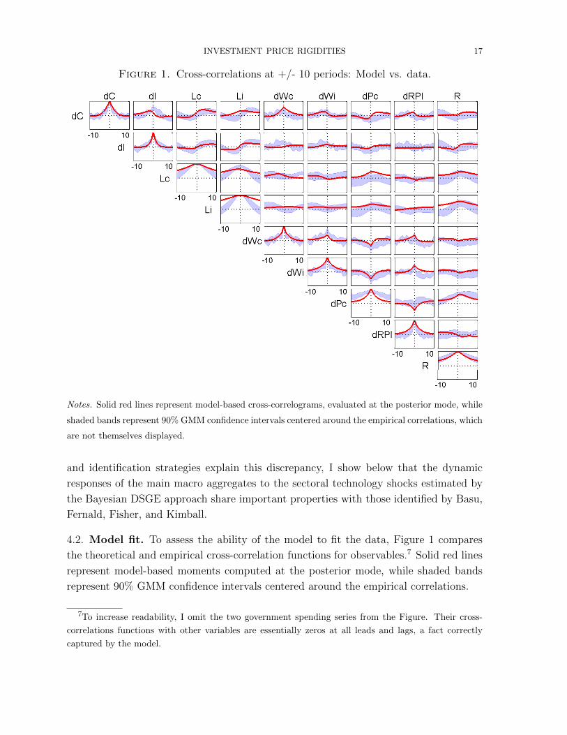
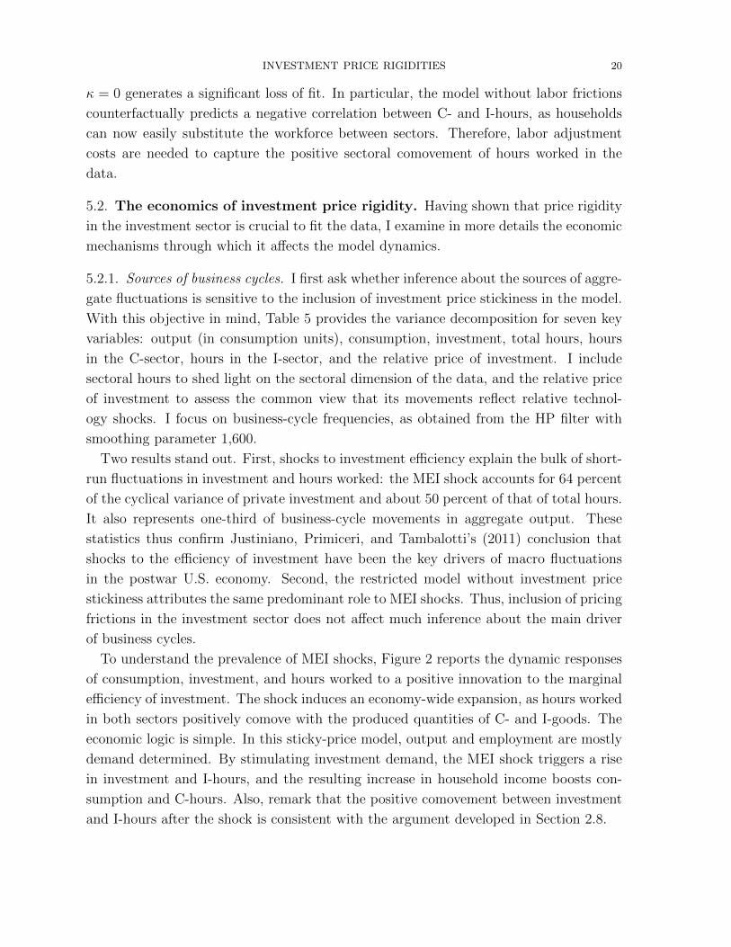
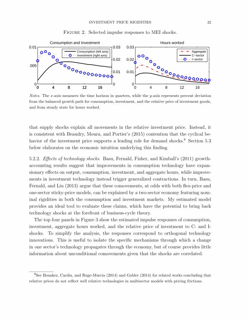
To understand the prevalence of MEI shocks, Figure 2 reports the dynamic responses
of consumption, investment, and hours worked to a positive innovation to the marginal
efficiency of investment. The shock induces an economy-wide expansion, as hours worked
in both sectors positively comove with the produced quantities of C- and I-goods. The
economic logic is simple. In this sticky-price model, output and employment are mostly
demand determined. By stimulating investment demand, the MEI shock triggers a rise
in investment and I-hours, and the resulting increase in household income boosts con-
sumption and C-hours. Also, remark that the positive comovement between investment
and I-hours after the shock is consistent with the argument developed in Section 2.8.

INVESTMENT PRICE RIGIDITIES 21
Table 5. Posterior variance decomposition at business-cycle frequencies.
Innovation lnXt lnCt ln It lnLt lnLct lnLit lnRPIt
MEI shock
ευ 29 13 64 49 16 52 4
C- and I-technology shocks
εµc, εµi 32 20 5 19 14 22 17
C-price markup shock
εηc 16 21 3 10 24 4 20
I-price markup shock
εηi 5 4 11 7 3 9 40
C-wage markup shock
εηwc 4 6 1 2 10 0 2
I-wage markup shock
εηwi 1 0 1 1 0 1 2
Preference shock
εζ 9 25 12 4 15 7 10
Monetary shock
εm 3 9 3 7 13 4 5
Government C- and I-spending shocks
εgc, εgi 1 1 0 2 5 1 0
Notes. Decomposition computed at the posterior mode using the HP filter with
smoothing parameter equal to 1, 600 to extract the business cycle. Because they
are correlated, the two technology shocks appear together. Columns may not sum
to 100 because of rounding errors.
While investment price rigidity has little effect on the estimated role of MEI shocks,
it matters more for assessing the contributions of technology shocks. According to the
complete model, they account for a moderate share of business-cycle movements but are
not negligible: together, they represent about 30 percent of the fluctuations in output
and 20 percent for consumption and hours worked. However, they do not explain much of
investment movements. Interestingly, these contributions are reversed when investment
pricing frictions are excluded from the model, as technology shocks then account for
26 percent of investment fluctuations but for only 10 percent of hours movements. As
discussed in Section 5.2.2 below, these divergent patterns originate from the strikingly
different effects of technology shocks when the model includes or excludes investment
price rigidity.
Finally, the last column in Table 5 shows that shocks to good-market markups account
for 60 percent of the cyclical volatility of the relative price of investment in the model,
while the contribution from technology shocks is much lower at 17 percent. This decom-
position is another key result, because it goes strongly against the standard assumption
INVESTMENT PRICE RIGIDITIES 22
Figure 2. Selected impulse responses to MEI shocks.
0 4 8 12 160
0.005
0.01Consumption and Investment
0 4 8 12 160
0.01
0.02
0.03Consumption (left axis)Investment (right axis)
0 4 8 12 160
0.01
0.02
0.03Hours worked
AggregateC−sectorI−sector
Notes. The x-axis measures the time horizon in quarters, while the y-axis represents percent deviation
from the balanced growth path for consumption, investment, and the relative price of investment goods,
and from steady state for hours worked.
that supply shocks explain all movements in the relative investment price. Instead, it
is consistent with Beaudry, Moura, and Portier’s (2015) contention that the cyclical be-
havior of the investment price supports a leading role for demand shocks.8 Section 5.3
below elaborates on the economic intuition underlying this finding.
5.2.2. Effects of technology shocks. Basu, Fernald, Fisher, and Kimball’s (2011) growth-
accounting results suggest that improvements in consumption technology have expan-
sionary effects on output, consumption, investment, and aggregate hours, while improve-
ments in investment technology instead trigger generalized contractions. In turn, Basu,
Fernald, and Liu (2013) argue that these comovements, at odds with both flex-price and
one-sector sticky-price models, can be explained by a two-sector economy featuring nom-
inal rigidities in both the consumption and investment markets. My estimated model
provides an ideal tool to evaluate these claims, which have the potential to bring back
technology shocks at the forefront of business-cycle theory.
The top four panels in Figure 3 show the estimated impulse responses of consumption,
investment, aggregate hours worked, and the relative price of investment to C- and I-
shocks. To simplify the analysis, the responses correspond to orthogonal technology
innovations. This is useful to isolate the specific mechanisms through which a change
in one sector’s technology propagates through the economy, but of course provides little
information about unconditional comovements given that the shocks are correlated.
8See Bouakez, Cardia, and Ruge-Murcia (2014) and Gabler (2014) for related works concluding that
relative prices do not reflect well relative technologies in multisector models with pricing frictions.

INVESTMENT PRICE RIGIDITIES 23
Remarkably, the estimated responses share important features with Basu, Fernald,
Fisher, and Kimball’s (2011) estimates. Positive C-shocks trigger expansions in con-
sumption and investment, while positive I-shocks push the economy into a severe reces-
sion. An important difference with Basu, Fernald, Fisher, and Kimball is that aggregate
hours fall on impact after a C-shock, while they obtain an increase (although not statis-
tically significant). Strikingly, both consumption and total hours worked stay depressed
for more than five years after improvements in I-technology, while investment initially
falls but recovers after about one year and a half. Overall, the correspondence with Basu,
Fernald, Fisher, and Kimball’s results, based on an unrelated empirical strategy, bolsters
confidence that C- and I-technology shocks as well as their propagation channels have
been correctly identified by the Bayesian DSGE approach.
The bottom two panels display the responses of C- and I-hours, allowing to clarify the
behavior of firms after technology shocks. Conditional on the responses of consumption
and investment, those of sectoral hours are not surprising in this demand-driven economy.
First, hours worked in the sector unaffected by the shock closely track the behavior of
the corresponding output, as illustrated by I-hours after a positive C-shock.9 This is
intuitive: if technology is unchanged, movements in output must be fully reflected in
inputs. Second, hours in the sector affected by the shock also follow their output, but
with a negative shift due to the less-than-proportional increase in demand after the
productivity rise induced by price stickiness. This is especially visible in the response
of I-hours to a positive I-shock: although investment increases steadily after about one
year and a half, I-hours stay depressed at all horizons because the rise in productivity is
sufficient to sustain higher production by itself.
Basu, Fernald, Fisher, and Kimball conclude from their results that C- and I-shocks
may be a major source of fluctuations in the U.S. economy, given that they both gen-
erate business-cycle-like comovements between consumption, investment, and hours. As
the variance decomposition from Table 5 shows, this contention is at odds with the es-
timated model, which instead favors MEI shocks. The intuition behind this prediction
follows from the estimated responses just discussed. In the aggregate, C-shocks trig-
ger negative short-run comovements between output and hours worked, while I-shocks
generate negative medium-run comovements between investment and both consumption
and hours. At the sectoral level, both shocks induce negative comovements between C-
and I-hours. Given these patterns, the time for a dramatic reevaluation of technology
shocks’ contribution to macro fluctuations may not have come yet.
9The impact rise in C-hours after the I-shock seems puzzling given the simultaneous fall in consump-
tion. It is in fact due to the one-shot jump in government expenditures on consumption goods induced
by the stochastic trend.
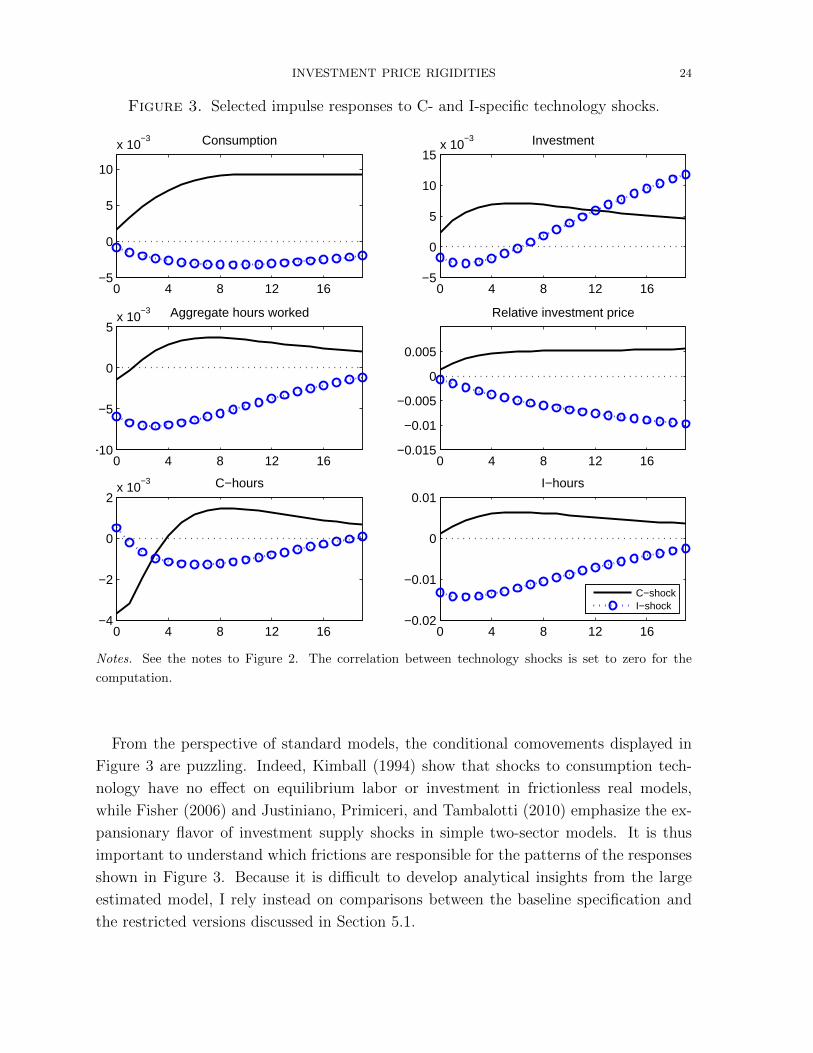
INVESTMENT PRICE RIGIDITIES 24
Figure 3. Selected impulse responses to C- and I-specific technology shocks.
0 4 8 12 16−5
0
5
10
x 10−3 Consumption
0 4 8 12 16−5
0
5
10
15x 10
−3 Investment
0 4 8 12 16−10
−5
0
5x 10
−3 Aggregate hours worked
0 4 8 12 16−0.015
−0.01
−0.005
0
0.005
Relative investment price
0 4 8 12 16−5
0
5
10
x 10−3 Consumption
0 4 8 12 16−5
0
5
10
15x 10
−3 Investment
0 4 8 12 16−10
−5
0
5x 10
−3 Aggregate hours worked
0 4 8 12 16−0.015
−0.01
−0.005
0
0.005
Relative investment price
0 4 8 12 16−4
−2
0
2x 10
−3 C−hours
0 4 8 12 16−0.02
−0.01
0
0.01I−hours
C−shockI−shock
Notes. See the notes to Figure 2. The correlation between technology shocks is set to zero for the
computation.
From the perspective of standard models, the conditional comovements displayed in
Figure 3 are puzzling. Indeed, Kimball (1994) show that shocks to consumption tech-
nology have no effect on equilibrium labor or investment in frictionless real models,
while Fisher (2006) and Justiniano, Primiceri, and Tambalotti (2010) emphasize the ex-
pansionary flavor of investment supply shocks in simple two-sector models. It is thus
important to understand which frictions are responsible for the patterns of the responses
shown in Figure 3. Because it is difficult to develop analytical insights from the large
estimated model, I rely instead on comparisons between the baseline specification and
the restricted versions discussed in Section 5.1.
INVESTMENT PRICE RIGIDITIES 25
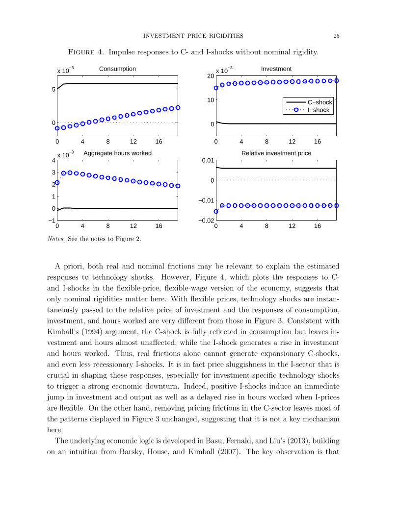
Figure 4. Impulse responses to C- and I-shocks without nominal rigidity.
0 4 8 12 16
0
5
x 10−3 Consumption
0 4 8 12 16
0
10
20x 10
−3 Investment
C−shockI−shock
0 4 8 12 16−1
0
1
2
3
4x 10
−3 Aggregate hours worked
0 4 8 12 16−0.02
−0.01
0
0.01Relative investment price
0 4 8 12 16
0
5
x 10−3 Consumption
0 4 8 12 16
0
10
20x 10
−3 Investment
C−shockI−shock
0 4 8 12 16−1
0
1
2
3
4x 10
−3 Aggregate hours worked
0 4 8 12 16−0.02
−0.01
0
0.01Relative investment price
Notes. See the notes to Figure 2.
A priori, both real and nominal frictions may be relevant to explain the estimated
responses to technology shocks. However, Figure 4, which plots the responses to C-
and I-shocks in the flexible-price, flexible-wage version of the economy, suggests that
only nominal rigidities matter here. With flexible prices, technology shocks are instan-
taneously passed to the relative price of investment and the responses of consumption,
investment, and hours worked are very different from those in Figure 3. Consistent with
Kimball’s (1994) argument, the C-shock is fully reflected in consumption but leaves in-
vestment and hours almost unaffected, while the I-shock generates a rise in investment
and hours worked. Thus, real frictions alone cannot generate expansionary C-shocks,
and even less recessionary I-shocks. It is in fact price sluggishness in the I-sector that is
crucial in shaping these responses, especially for investment-specific technology shocks
to trigger a strong economic downturn. Indeed, positive I-shocks induce an immediate
jump in investment and output as well as a delayed rise in hours worked when I-prices
are flexible. On the other hand, removing pricing frictions in the C-sector leaves most of
the patterns displayed in Figure 3 unchanged, suggesting that it is not a key mechanism
here.
The underlying economic logic is developed in Basu, Fernald, and Liu’s (2013), building
on an intuition from Barsky, House, and Kimball (2007). The key observation is that
INVESTMENT PRICE RIGIDITIES 26
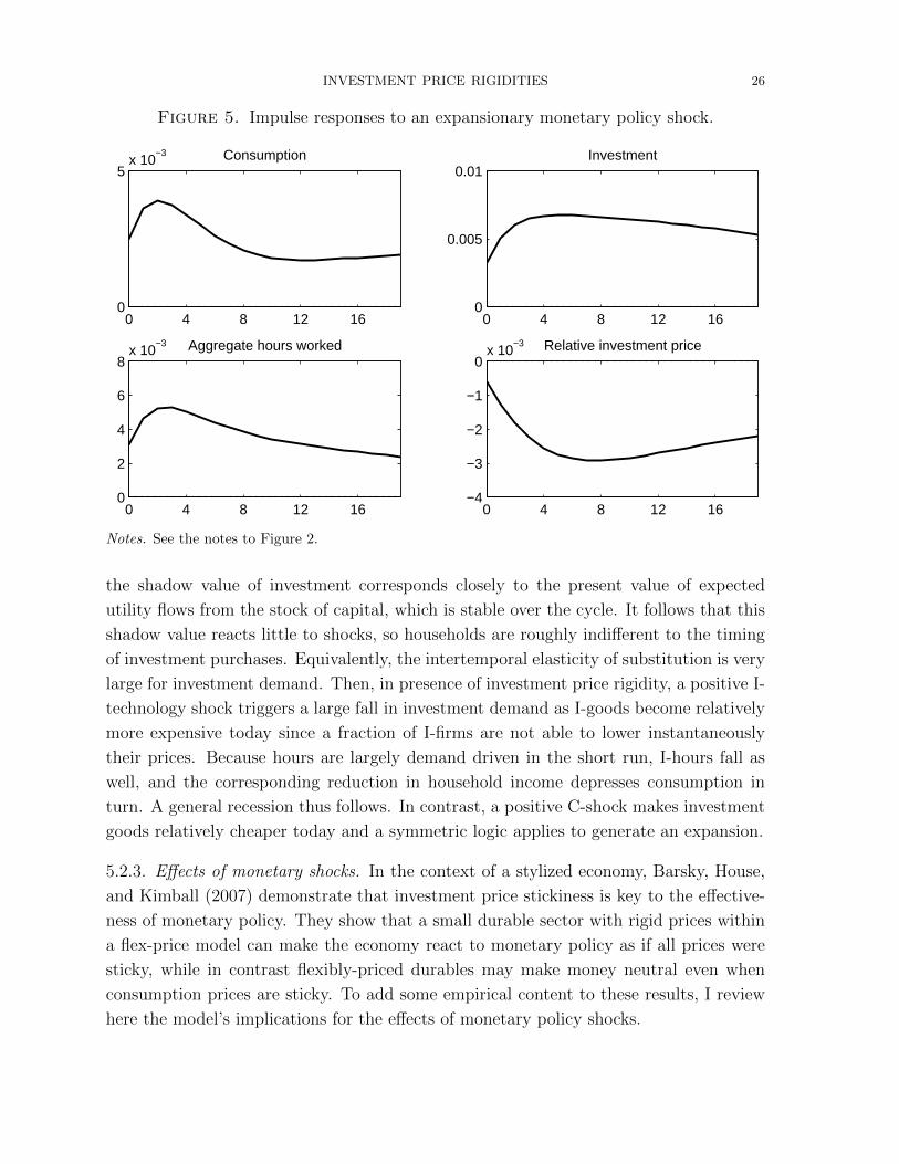
Figure 5. Impulse responses to an expansionary monetary policy shock.
0 4 8 12 160
5x 10
−3 Consumption
0 4 8 12 160
0.005
0.01Investment
0 4 8 12 160
2
4
6
8x 10
−3 Aggregate hours worked
0 4 8 12 16−4
−3
−2
−1
0x 10
−3 Relative investment price
0 4 8 12 160
5x 10
−3 Consumption
0 4 8 12 160
0.005
0.01Investment
0 4 8 12 160
2
4
6
8x 10
−3 Aggregate hours worked
0 4 8 12 16−4
−3
−2
−1
0x 10
−3 Relative investment price
Notes. See the notes to Figure 2.
the shadow value of investment corresponds closely to the present value of expected
utility flows from the stock of capital, which is stable over the cycle. It follows that this
shadow value reacts little to shocks, so households are roughly indifferent to the timing
of investment purchases. Equivalently, the intertemporal elasticity of substitution is very
large for investment demand. Then, in presence of investment price rigidity, a positive I-
technology shock triggers a large fall in investment demand as I-goods become relatively
more expensive today since a fraction of I-firms are not able to lower instantaneously
their prices. Because hours are largely demand driven in the short run, I-hours fall as
well, and the corresponding reduction in household income depresses consumption in
turn. A general recession thus follows. In contrast, a positive C-shock makes investment
goods relatively cheaper today and a symmetric logic applies to generate an expansion.
5.2.3. Effects of monetary shocks. In the context of a stylized economy, Barsky, House,
and Kimball (2007) demonstrate that investment price stickiness is key to the effective-
ness of monetary policy. They show that a small durable sector with rigid prices within
a flex-price model can make the economy react to monetary policy as if all prices were
sticky, while in contrast flexibly-priced durables may make money neutral even when
consumption prices are sticky. To add some empirical content to these results, I review
here the model’s implications for the effects of monetary policy shocks.

INVESTMENT PRICE RIGIDITIES 27
Figure 5 reports selected estimated impulse responses to monetary policy shock low-
ering the nominal interest rate. The shock is clearly expansionary, as consumption,
investment, and aggregate hours worked all increase together. At the sectoral level, both
C- and I-hours rise simultaneously. Also, the relative price of investment falls for several
periods, reflecting the ability of C-firms to increase their prices faster than I-firms in
response to the increase in demand. Overall, the economy’s dynamics after a monetary
shock resemble a lot those from a one-sector model with sticky prices.
In light of Barsky, House, and Kimball’s (2007) analysis, an interesting question is thus
that of the relative role of consumption and investment price rigidities in shaping those
dynamics. In fact, both constitute here quite equivalent mechanisms, probably because
the estimated Calvo parameters are high in both sectors. Suppressing pricing frictions in
one sector while leaving them in the other has little effects on the movements displayed
in Figure 5. The only noticeable changes are a fall in the persistence of the responses
of consumption, investment, and hours worked when prices are rigid in a single sector,
and a switch in the sign of the response of the relative price of investment depending on
which sector is able to instantaneously adjusts. On the other hand, suppressing nominal
frictions in both sectors unsurprisingly makes monetary policy almost neutral.
5.3. Shocks and the relative price of investment. Following Greenwood, Hercowitz,
and Krusell (2000), it is common to identify shocks to the relative technology between
the C- and I-sectors using the relative price of investment. The literature has considered
essentially two practical implementations, either based on a period-by-period mapping
between the two series (Justiniano, Primiceri, and Tambalotti, 2011; Schmitt-Grohe and
Uribe, 2012) or on long-run restrictions (Fisher, 2006). By allowing for investment price
rigidity and relaxing the standard assumption of perfect pass-through of relative tech-
nology shocks to the relative price, this paper’s model allows to evaluate these empirical
strategies.
As discussed in Section 5.2.1, C- and I-technology shocks account for only one fifth of
the cyclical variance of the relative price of investment according to the model, while the
contribution of price markup shocks is above 50 percent. These respective shares follow
from the large estimated Calvo coefficients in both the consumption and investment
markets. The inflation equation in the consumption sector may be written as
lnπc,t − ιpc lnπc,t−1 = ΘpcEt
∞∑j=0
(βµ1−σ)j lnmcct+j + Et
∞∑j=0
(βµ1−σ)j ln ηct+j,
where Θpc = (1− ξpc)(1− βµ1−σξpc)/ξpc is a function of structural model parameters —
including the Calvo coefficient ξpc —, µ denotes the average growth rate of the economy,
mcct is the real marginal cost in the C-sector, and ηct is the price markup shock in the
INVESTMENT PRICE RIGIDITIES 28
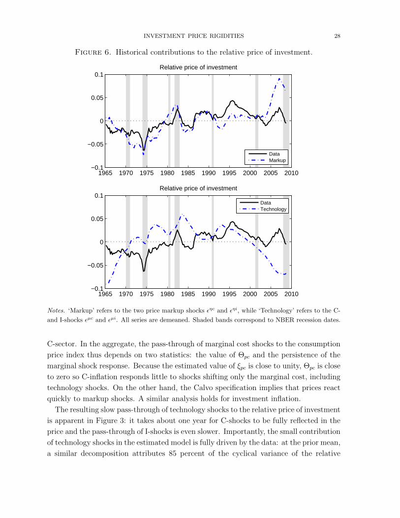
Figure 6. Historical contributions to the relative price of investment.
Relative price of investment
1965 1970 1975 1980 1985 1990 1995 2000 2005 2010−0.1
−0.05
0
0.05
0.1
DataMarkup
Relative price of investment
1965 1970 1975 1980 1985 1990 1995 2000 2005 2010−0.1
−0.05
0
0.05
0.1DataTechnology
Relative price of investment
1965 1970 1975 1980 1985 1990 1995 2000 2005 2010−0.1
−0.05
0
0.05
0.1
DataMarkup
Relative price of investment
1965 1970 1975 1980 1985 1990 1995 2000 2005 2010−0.1
−0.05
0
0.05
0.1DataTechnology
Notes. ‘Markup’ refers to the two price markup shocks εηc and εηi, while ‘Technology’ refers to the C-
and I-shocks εµc and εµi. All series are demeaned. Shaded bands correspond to NBER recession dates.
C-sector. In the aggregate, the pass-through of marginal cost shocks to the consumption
price index thus depends on two statistics: the value of Θpc and the persistence of the
marginal shock response. Because the estimated value of ξpc is close to unity, Θpc is close
to zero so C-inflation responds little to shocks shifting only the marginal cost, including
technology shocks. On the other hand, the Calvo specification implies that prices react
quickly to markup shocks. A similar analysis holds for investment inflation.
The resulting slow pass-through of technology shocks to the relative price of investment
is apparent in Figure 3: it takes about one year for C-shocks to be fully reflected in the
price and the pass-through of I-shocks is even slower. Importantly, the small contribution
of technology shocks in the estimated model is fully driven by the data: at the prior mean,
a similar decomposition attributes 85 percent of the cyclical variance of the relative
INVESTMENT PRICE RIGIDITIES 29
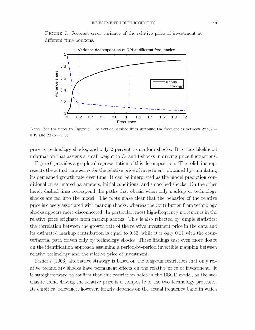
Figure 7. Forecast error variance of the relative price of investment at
different time horizons.
0 0.2 0.4 0.6 0.8 1 1.2 1.4 1.6 1.8 20
0.2
0.4
0.6
0.8
1Variance decomposition of RPI at different frequencies
Frequency
Var
ianc
e sh
are
MarkupTechnology
Notes. See the notes to Figure 6. The vertical dashed lines surround the frequencies between 2π/32 =
0.19 and 2π/6 = 1.05.
price to technology shocks, and only 2 percent to markup shocks. It is thus likelihood
information that assigns a small weight to C- and I-shocks in driving price fluctuations.
Figure 6 provides a graphical representation of this decomposition. The solid line rep-
resents the actual time series for the relative price of investment, obtained by cumulating
its demeaned growth rate over time. It can be interpreted as the model prediction con-
ditional on estimated parameters, initial conditions, and smoothed shocks. On the other
hand, dashed lines correspond the paths that obtain when only markup or technology
shocks are fed into the model. The plots make clear that the behavior of the relative
price is closely associated with markup shocks, whereas the contribution from technology
shocks appears more disconnected. In particular, most high-frequency movements in the
relative price originate from markup shocks. This is also reflected by simple statistics:
the correlation between the growth rate of the relative investment price in the data and
its estimated markup contribution is equal to 0.82, while it is only 0.11 with the coun-
terfactual path driven only by technology shocks. These findings cast even more doubt
on the identification approach assuming a period-by-period invertible mapping between
relative technology and the relative price of investment.
Fisher’s (2006) alternative strategy is based on the long-run restriction that only rel-
ative technology shocks have permanent effects on the relative price of investment. It
is straightforward to confirm that this restriction holds in the DSGE model, as the sto-
chastic trend driving the relative price is a composite of the two technology processes.
Its empirical relevance, however, largely depends on the actual frequency band in which

INVESTMENT PRICE RIGIDITIES 30
technology shocks are the leading contributors to the variance of the relative investment
price. To take an extreme example, if technology disturbances dominate only in frequen-
cies lower than 100 years, the long-run restriction would be of little practical use given
the sample sizes typically available for macro series.
To shed light on this issue, Figure 7 plots the respective contributions of markup and
technology shocks to the variance of the relative price of investment at different spectrum
frequencies. The two vertical lines surround the frequency band commonly associated
with business cycles, corresponding to 6 to 32 quarters. Echoing the statistics in Table
5, markup shocks are the leading sources of fluctuations in the relative price at business-
cycle frequencies, and also at higher frequencies. On the other hand, technology shocks
dominate at frequencies close to zero, reflecting the nonstationary behavior of the tech-
nological trend. The cutoff frequency for the lead of technology shocks is close to 36
quarters, or about 15 years. Given that available samples exceed by large such a time
span, one could view this finding as providing some support in favor of long-run restric-
tions. However, Monte-Carlo experiments would be helpful to assess the robustness of
this conclusion, for instance using the estimated DSGE model as data generating pro-
cess in a simulation framework similar to Erceg, Guerrieri, and Gust (2005), Christiano,
Eichenbaum, and Vigfusson (2007), or Chari, Kehoe, and McGrattan (2008).
6. Conclusion
This paper introduces sector-specific nominal rigidities and frictions in factor realloca-
tion in a quantitative two-sector DSGE model. Bayesian estimation from quarterly U.S.
data shows that such mechanisms are important to fit the data. In particular, I make
an empirical contribution to the DSGE literature by showing the importance of price
rigidities in the investment sector, which have been mostly ignored so far.
The model sheds new light on standard macroeconomics issues. For instance, I find
that technology shocks account for only one third of the movements in the relative
price of investment, calling into question the validity of a widespread identification ap-
proach. Also, consistent with the growth accounting literature, the model predicts that
improvements in consumption technology generate an expansion while improvements in
investment technology trigger deep recessions. Overall, a core message of the paper is
that the DSGE literature has much to gain by paying more attention to the sectoral
dimension of the data, which provides both new economic mechanisms and a relevant
source of empirical information.

INVESTMENT PRICE RIGIDITIES 31
References
Barsky, R. B., C. L. House, and M. S. Kimball (2007): “Sticky-Price Models and
Durable Goods,” American Economic Review, 97(3), 984–998.
Basu, S., J. G. Fernald, J. D. Fisher, and M. S. Kimball (2011): “Sector-
Specific Technical Change,” Unpublished manuscript, Federal Reserve Bank of San
Francisco.
Basu, S., J. G. Fernald, and Z. Liu (2013): “Technology Shocks in a Two-Sector
DSGE Model,” Unpublished manuscript, Federal Reserve Bank of San Francisco.
Beaudry, P., A. Moura, and F. Portier (2015): “Reexamining the Cyclical Be-
havior of the Relative Price of Investment,” Economics Letters, 135(C), 108–111.
Bils, M., and P. J. Klenow (2004): “Some Evidence on the Importance of Sticky
Prices,” Journal of Political Economy, 112(5), 947–985.
Bouakez, H., E. Cardia, and F. Ruge-Murcia (2014): “Sectoral Price Rigidity
and Aggregate Dynamics,” European Economic Review, 65(C), 1–22.
Calvo, G. A. (1983): “Staggered Prices in a Utility-Maximizing Framework,” Journal
of Monetary Economics, 12(3), 383–398.
Case, K. E., and R. J. Shiller (1989): “The Efficiency of the Market for Single-
Family Homes,” American Economic Review, 79(1), 125–37.
Chari, V., P. J. Kehoe, and E. R. McGrattan (2008): “Are structural VARs with
long-run restrictions useful in developing business cycle theory?,” Journal of Monetary
Economics, 55(8), 1337–1352.
Christiano, L. J., M. Eichenbaum, and C. L. Evans (2005): “Nominal Rigidities
and the Dynamic Effects of a Shock to Monetary Policy,” Journal of Political Economy,
113(1), 1–45.
Christiano, L. J., M. Eichenbaum, and R. Vigfusson (2007): “Assessing Struc-
tural VARs,” in NBER Macroeconomics Annual 2006, Volume 21, pp. 1–106. National
Bureau of Economic Research, Inc.
Eichenbaum, M., and J. D. Fisher (2007): “Estimating the Frequency of Price Re-
Optimization in Calvo-Style Models,” Journal of Monetary Economics, 54(7), 2032–
2047.
Erceg, C. J., L. Guerrieri, and C. Gust (2005): “Can Long-Run Restrictions
Identify Technology Shocks?,” Journal of the European Economic Association, 3(6),
1237–1278.
Fisher, J. D. (2006): “The Dynamic Effects of Neutral and Investment-Specific Tech-
nology Shocks,” Journal of Political Economy, 114(3), 413–451.
INVESTMENT PRICE RIGIDITIES 32
Gabler, A. (2014): “Relative Price Fluctuations in a Multi-Sector Model with Imper-
fect Competition,” Review of Economic Dynamics, 17(3), 474–483.
Galı, J. (1999): “Technology, Employment, and the Business Cycle: Do Technology
Shocks Explain Aggregate Fluctuations?,” American Economic Review, 89(1), 249–
271.
Greenwood, J., Z. Hercowitz, and P. Krusell (2000): “The Role of Investment-
Specific Technological Change in the Business Cycle,” European Economic Review,
44(1), 91–115.
Horvath, M. (2000): “Sectoral Shocks and Aggregate Fluctuations,” Journal of Mon-
etary Economics, 45(1), 69–106.
Iacoviello, M. (2010): “Housing in DSGE Models: Findings and New Directions,”
in Housing Markets in Europe: A Macroeconomic Perspective, ed. by O. de Bandt,
T. Knetsch, J. P. nalosa, and F. Zollino, pp. 3–16. Springer-Verlag.
Iacoviello, M., and S. Neri (2010): “Housing Market Spillovers: Evidence from
an Estimated DSGE Model,” American Economic Journal: Macroeconomics, 2(2),
125–64.
Justiniano, A., G. Primiceri, and A. Tambalotti (2010): “Investment Shocks
and Business Cycles,” Journal of Monetary Economics, 57, 132–145.
(2011): “Investment Shocks and the Relative Price of Investment,” Review of
Economic Dynamics, 14(1), 101–121.
Kehoe, P. J., and V. Midrigan (2010): “Prices are Sticky After All,” NBER Working
Papers 16364, National Bureau of Economic Research, Inc.
Kim, J. (2003): “Functional Equivalence Between Intertemporal and Multisectoral In-
vestment Adjustment Costs,” Journal of Economic Dynamics and Control, 27(4), 533–
549.
Kimball, M. S. (1994): “Proof of Consumption Sector Neutrality,” Unpublished man-
uscript, University of Michigan.
Rıos-Rull, J.-V., F. Schorfheide, C. Fuentes-Albero, M. Kryshko, and
R. Santaeulalia-Llopis (2012): “Methods versus Substance: Measuring the Ef-
fects of Technology Shocks,” Journal of Monetary Economics, 59(8), 826–846.
Schmitt-Grohe, S., and M. Uribe (2012): “What’s News in Business Cycles?,”
Econometrica, 80(6), 2733–2764.
Smets, F., and R. Wouters (2007): “Shocks and Frictions in US Business Cycles: A
Bayesian DSGE Approach,” American Economic Review, 97(3), 586–606.
Sullivan, D. (1997): “Trends in Real Wage Growth,” Chicago Fed Letter, 115.
Woodford, M. (2003): Interest and Prices: Foundations of a Theory of Monetary
Policy. Princeton University Press, Princeton, New Jersey, USA.

INVESTMENT PRICE RIGIDITIES 33
Appendix A. Data and Sources
This appendix provides data sources and describes the construction of observable
variables used in estimation. All quantity series are converted to per-capita terms using
the population series provided by the Bureau of Economic Analysis (BEA) in its National
Income and Product Accounts (NIPA, Table 2.1, line 40).
Consumption: Quantity and price series. I define nominal consumption as nominal con-
sumption expenditures on nondurable goods and services (BEA, NIPA Table 1.1.5, lines
5 and 6). The corresponding quantity series are provided by the BEA (NIPA Table 1.1.6,
lines 5 and 6). I construct the aggregate consumption quantity and price series, Ct and
P ct , by chain aggregation.
Investment: Quantity and price series. Nominal investment is the sum of nominal con-
sumption expenditures on durable goods and nominal fixed investment (BEA, NIPA
Table 1.1.5, lines 4 and 8). The corresponding quantity series are provided by the BEA
(NIPA Table 1.1.6, lines 4 and 8). I construct the aggregate investment quantity and
price series, It and P it , by chain aggregation.
Government consumption and investment. Nominal government consumption expendi-
tures and nominal gross government investment are provided by the BEA (NIPA Table
3.9.5, lines 2 and 3). I construct real government consumption and real government
investment, Gct and Gi
t, by deflating each series by the corresponding chain-aggregated
price index.
Hours worked. The Bureau of Labor Statistics (BLS) provides series on employment
and average hours worked for the nonfarm business sector (CES0500000007), construc-
tion (CES2000000007), durable manufacturing (CES3100000007), and professional and
business services (CES6000000007). For each of these sectors, I compute total hours as
the product of employment and average hours.
I define investment hours, Lit, as the sum of hours worked in construction, durable
manufacturing, and professional and business services. I include the latter sector because
more than 50 percent of its output is allocated to investment according to U.S. input-
output tables. The paper’s findings are not sensitive to this inclusion. I then define
consumption hours, Lct , as the difference between total hours in the nonfarm business
sector and investment hours.
Wages. The BLS also provides series on nominal hourly compensation for each of the
above sectors. To construct the relevant nominal wage rates, I first compute total wage

INVESTMENT PRICE RIGIDITIES 34
bills by multiplying total hours and hourly compensation. I then split the aggregate wage
bill for the nonfarm business sector between consumption and investment, using the same
classification as for hours worked. Eventually, I compute the nominal consumption and
investment wage series, W ct and W i
t , by dividing the two sectoral wage bills by the
corresponding hours series.
Inflation and the relative price of investment. Inflation in the consumption sector, πct ,
is defined as the growth rate in the chain-aggregated consumption price index P ct . The
relative price of investment goods, RPIt, is defined as P it /P
ct .
Interest rate. The nominal interest rate, Rt, is measured as the quarterly average of the
effective Federal Funds rate expressed in quarterly units.