Embed Size (px)
Citation preview
Understanding the relationship between
business failure and macroeconomic
business cycles: a focus on South African
businesses
Marinus de Jager Student Number: 1558046
Dr. José Barreira Supervisor
A research report submitted to the Faculty of Commerce, Law and
Management, University of the Witwatersrand, in partial fulfilment of the
requirements for the degree of Master of Management, specialising in
Entrepreneurship and New Venture Creation
Johannesburg, 2017
ii
ABSTRACT
This study examined the relationship between business failure and
macroeconomic fluctuations within business cycles of South Africa’s economy
for the time period 1980 to 2016. The study also sought to understand where, if
any, immediate and lag correlations between fluctuations and business failure
could be established. To understand this connection, this study used
longitudinal data sets of different macroeconomic factors and studied their
influence on business failure. The vector error correction model (VECM) was
used to determine the long-term relationship between failure and each of the
other variables. Additionally, Granger Causality was applied to establish
whether the macroeconomic variables investigated in this study can be
constructed to predict the probability of business failures.
Three classes of macroeconomic predictor variables were considered. Firstly,
well-known international variables in the form of GDP and CPI were used.
Secondly, the study incorporated the three Composite Business Cycle
indicators- leading, coincident and lagging. Lastly, behavioural indicators were
used to incorporate the views of the actual businesses and their customers,
which for this the study were the Business and Consumer Confidence Indices.
After examining the effects the 7 macroeconomic variables had on business
failure, the study found that there is a long-run relationship between the
Composite Lagging Business Cycle indicator, the Business Confidence and
Consumer confidence, which influenced Business Failure. Additionally, it was
noted that Business Failure influence the Composite Lagging Business Cycle
indicator in the long-run. The study additionally found that Business Failure may
Granger Cause the Composite Leading Business Cycle indicator
Outcomes of the study are potentially vital for entrepreneurs to understand the
timing of entry into markets based on macroeconomic fluctuations through their
cycles in certain industries. Business owners can make proactive financial and
strategic decisions vital for survival of their business through the expansion and
especially in the contraction cycles of the macroeconomic environments.
iii
DISCLAIMER
The acceptance or use of the information provided in this report will in no way
relieve the users of their responsibilities in terms of any problem resolution,
prescription or accountability for decisions they take in managing their
processes. The users shall satisfy themselves that the principles and
recommendations used and/or selected are always suitable to meet their
respective circumstances and contexts. The onus of ensuring that the principles
and recommendations fit the purpose shall at all times rest with the user.
Nonetheless, the sole purpose of the information contained in this report is for
guidance and educational purposes.
All statements, comments or opinions expressed in this research report are
those of the author and do not necessarily represent the opinions, or reflect the
official position, of the University of Witwatersrand or the author’s employers.
COPYRIGHT
Except for normal review purposes, no part of this report may be reproduced or
used in any form or by any means electronic or mechanical, including
photocopying and recording or by any information storage or retrieval system,
without the written consent of the author or the University of the Witwatersrand.

iv
DECLARATION
I, Marinus de Jager, declare that this research report is my own work except as
indicated in the references and acknowledgements. It is submitted in partial
fulfilment of the requirements for the degree of Master of Management from the
University of the Witwatersrand, Johannesburg. It has not been submitted
before for any degree or examination in this or any other university.
Signed at …………………………………………………………………….…………
On the …………………………………….. day of ……..……………….2017

v
DEDICATION
I dedicate my research report to my family and many friends. A special feeling
of gratitude to my loving and caring wife, Chantelle, whose words of
encouragement and push for persistence kept me going. During this degree my
wife and I was blessed with a healthy boy, Miller, whom put a smile on our faces
when the tough got going.
I also dedicate this thesis to my colleagues who have supported me throughout
the process as well as my employer who made this possible. I will always
appreciate all they have done, especially Karen for whenever I needed help,
from printing to spell checking. Additionally I would like to thank Dr Yudhvir
Seetharam for assisting me with the framework and models for the statistical
analysis.
Ultimately this would not have been possible without the grace of God: “…but
he said to me, “My grace is sufficient for you, for my power is made perfect in
weakness.” Therefore I will boast all the more gladly about my weaknesses, so
that Christ’s power may rest on me” 2 Corinthians 12:9

vi
ACKNOWLEDGEMENTS
Writing this research paper would not have been without the help and support of
the kind people around me, to only some of whom it is possible to give
particular mention here. Thank you for Keerti Musunuri who made the statistical
analysis possible and Sarah Kaip for editing and proofreading.
On the very outset of this report, I would like to extend my sincere and heartfelt
appreciation towards the Business School, the Management, support within the
faculty, and all the people who have helped me in this endeavour. Without their
guidance, help and encouragement, I would not have made headway in the
paper.
I am ineffably indebted to Dr José Barrera for his conscientious guidance and
encouragement to accomplish this assignment.
I am extremely thankful to all the lecturers at the Business School who have
guided us every step of the way.
Any omission in this brief acknowledgment does not mean lack of gratitude.
vii
TABLE OF CONTENTS
ABSTRACT ....................................................................................................... II
DEDICATION ..................................................................................................... V
ACKNOWLEDGEMENTS ................................................................................. VI
TABLE OF CONTENTS .................................................................................. VII
LIST OF TABLES .............................................................................................. X
LIST OF FIGURES ............................................................................................ X
LIST OF ACRONYMS AND DEFINITIONS ...................................................... XI
1 CHAPTER 1: INTRODUCTION .............................................................. 1
1.1 INTRODUCTION .......................................................................................... 1
1.2 BACKGROUND OF THE STUDY ..................................................................... 3
1.3 THE CONTEXT OF THE PROBLEM .................................................................. 3
1.4 STATEMENT OF THE PROBLEM ..................................................................... 4 1.4.1 MAIN PROBLEM ................................................................................ 5 1.4.2 SUB PROBLEM ................................................................................. 5
1.5 SIGNIFICANCE OF THE STUDY ...................................................................... 5
1.6 DELIMITATIONS OF THE STUDY .................................................................... 6
1.7 DEFINITION OF TERMS ................................................................................ 6 1.7.1 SOUTH AFRICAN COMPANIES ............................................................ 6 1.7.2 MACROECONOMICS .......................................................................... 6 1.7.3 GDP (GROSS DOMESTIC PRODUCT) ................................................. 7 1.7.4 CPI (CONSUMER PRICE INDEX) ........................................................ 7 1.7.5 BCI (BUSINESS CONFIDENCE INDEX) ................................................. 7 1.7.6 CCI (CONSUMER CONFIDENCE INDEX) .............................................. 7 1.7.7 COMPOSITE BUSINESS CYCLE INDICATORS ........................................ 8 1.7.8 BUSINESS FAILURE ........................................................................... 8 1.7.9 BUSINESS CYCLES ........................................................................... 9
1.8 ASSUMPTIONS ......................................................................................... 10
2 CHAPTER 2: LITERATURE REVIEW .................................................. 11
2.1 INTRODUCTION ........................................................................................ 11
2.2 BUSINESS FAILURE .................................................................................. 11
2.3 THE THEORETICAL UNDERPINNINGS OF BUSINESS FAILURE ......................... 12
viii
2.4 THE SYMPTOMS OF BUSINESS FAILURE ..................................................... 13
2.5 CAUSES OF BUSINESS FAILURE ................................................................. 15 2.5.1 ENDOGENOUS CAUSES .................................................................. 15 2.5.2 EXOGENOUS FACTORS ................................................................... 18
2.6 MACROECONOMIC EFFECTS ON BUSINESS FAILURE .................................... 18
2.7 ECONOMIC PERFORMANCE OF THE COUNTRY ............................................ 20
2.8 BUSINESS CYCLES ................................................................................... 22 2.8.1 BREAKING DOWN THE BUSINESS CYCLE ........................................... 26 2.8.2 BUSINESS CYCLES AND GLOBAL INTERCONNECTEDNESS .................. 27 2.8.3 THE GLOBAL BUSINESS CYCLE AND ITS CHANGING DYNAMICS ............. 28
2.9 HYPOTHESIS STATEMENT .......................................................................... 30
2.10 CONCEPTUAL FRAMEWORK MODEL ............................................................ 31
3 CHAPTER 3: RESEARCH METHODOLOGY ...................................... 32
3.1 RESEARCH STRATEGY AND DESIGN ........................................................... 32
3.1.1. EPISTEMOLOGY AND ONTOLOGY ................................................................. 32 3.1.1.1. EPISTEMOLOGY ........................................................................... 32 3.1.2 ONTOLOGY .................................................................................... 34
3.2 CONCEPTUAL FRAMEWORK AND THE DATA ................................................ 36 3.2.1 BUSINESS FAILURE RATE ............................................................... 36 3.2.2 MACROECONOMIC FACTORS ........................................................... 36
3.3 THE POPULATION AND DATA ..................................................................... 40 3.3.1 QUARTERLY DATA .......................................................................... 40 3.3.2 BUSINESS FAILURE ........................................................................ 40 3.3.3 GDP ............................................................................................ 41 3.3.4 COMPOSITE BUSINESS CYCLE INDICATORS ...................................... 41 3.3.5 CONSUMER PRICE INDEX (CPI) ...................................................... 43 3.3.6 BUSINESS CONFIDENCE ................................................................. 43 3.3.7 CONSUMER CONFIDENCE ............................................................... 43
3.4 METHODS................................................................................................ 44
3.5 MODEL STRATEGY ................................................................................... 44 3.5.1 AUGMENTED DICKEY FULLER (ADF) TEST FOR STATIONARITY .......... 44 3.5.2 THE JOHANSEN TEST FOR CO-INTEGRATION .................................... 45 3.5.3 THE VECTOR ERROR CORRECTION MODEL (VCEM) ........................ 45 3.5.4 GRANGER CAUSALITY .................................................................... 46
3.6 LIMITATIONS OF DATASETS ........................................................................ 47
3.7 THE VALIDITY AND RELIABILITY OF RESEARCH ............................................. 47 3.7.1 VALIDITY ....................................................................................... 47 3.7.2 RELIABILITY ................................................................................... 49 3.7.3 ETHICAL CONSIDERATIONS ............................................................. 49
4 CHAPTER 4: PRESENTATION OF RESULTS .................................... 50
4.1 DATA PREPARATION ................................................................................. 51
ix
4.1.1 INTERPOLATING DATA ..................................................................... 51 4.1.2 TIME SERIES PLOTS ........................................................................ 51 4.1.3 THE AUGMENTED DICKEY-FULLER (ADF) TEST FOR STATIONARITY ... 52 4.1.4 SMOOTHENING .............................................................................. 55 4.1.5 LAG DETERMINATION ..................................................................... 56 4.1.6 COINTEGRATION, VECM AND GRANGER CAUSALITY TESTS .............. 60
4.2 HYPOTHESIS RESULTS ............................................................................. 61 4.2.1 HYPOTHESIS 1: CPI CAUSES BUSINESS FAILURE ............................... 61 4.2.2 HYPOTHESIS 5: GDP CAUSES BUSINESS FAILURE ............................ 64 4.2.3 HYPOTHESIS 2: CBCL CAUSES BUSINESS FAILURE ........................... 68 4.2.4 HYPOTHESIS 3: CBCC CAUSES BUSINESS FAILURE........................... 71 4.2.5 HYPOTHESIS 4: CBCG CAUSES BUSINESS FAILURE ......................... 74 4.2.6 HYPOTHESIS 6: BCI CAUSES BUSINESS FAILURE .............................. 77 4.2.7 HYPOTHESIS 7: CCI CAUSES BUSINESS FAILURE .............................. 81
5 CHAPTER 5: DISCUSSION OF THE RESULTS .................................. 85
5.1 INTRODUCTION ........................................................................................ 85
5.2 MODELS USED IN THE STUDY ..................................................................... 86 5.2.1 AUGMENTED DICKEY FULLER TEST ................................................. 86 5.2.2 THE JOHANSEN TEST FOR CO-INTEGRATION .................................... 90 5.2.3 THE VECTOR ERROR CORRECTION MODEL (VCEM) ........................ 91 5.2.4 GRANGER CAUSALITY .................................................................... 92
5.3 SUMMARY OF FINDINGS ............................................................................ 93
5.4 CONCLUSION ........................................................................................... 95
6 CHAPTER 6: CONCLUSIONS OF THE STUDY .................................. 99
6.1 INTRODUCTION ........................................................................................ 99
6.2 CONCLUSIONS OF THE STUDY ................................................................... 99
6.3 IMPLICATIONS AND RECOMMENDATIONS ................................................... 101
6.4 SUGGESTIONS FOR FURTHER RESEARCH ................................................. 104 6.4.1 ON A GOVERNMENTAL LEVEL ......................................................... 104 6.4.2 ON A MACRO LEVEL ...................................................................... 104 6.4.3 ON THE BUSINESS LEVEL .............................................................. 105 6.4.4 AT AN INDUSTRY LEVEL................................................................. 108
REFERENCES: ............................................................................................. 109
x
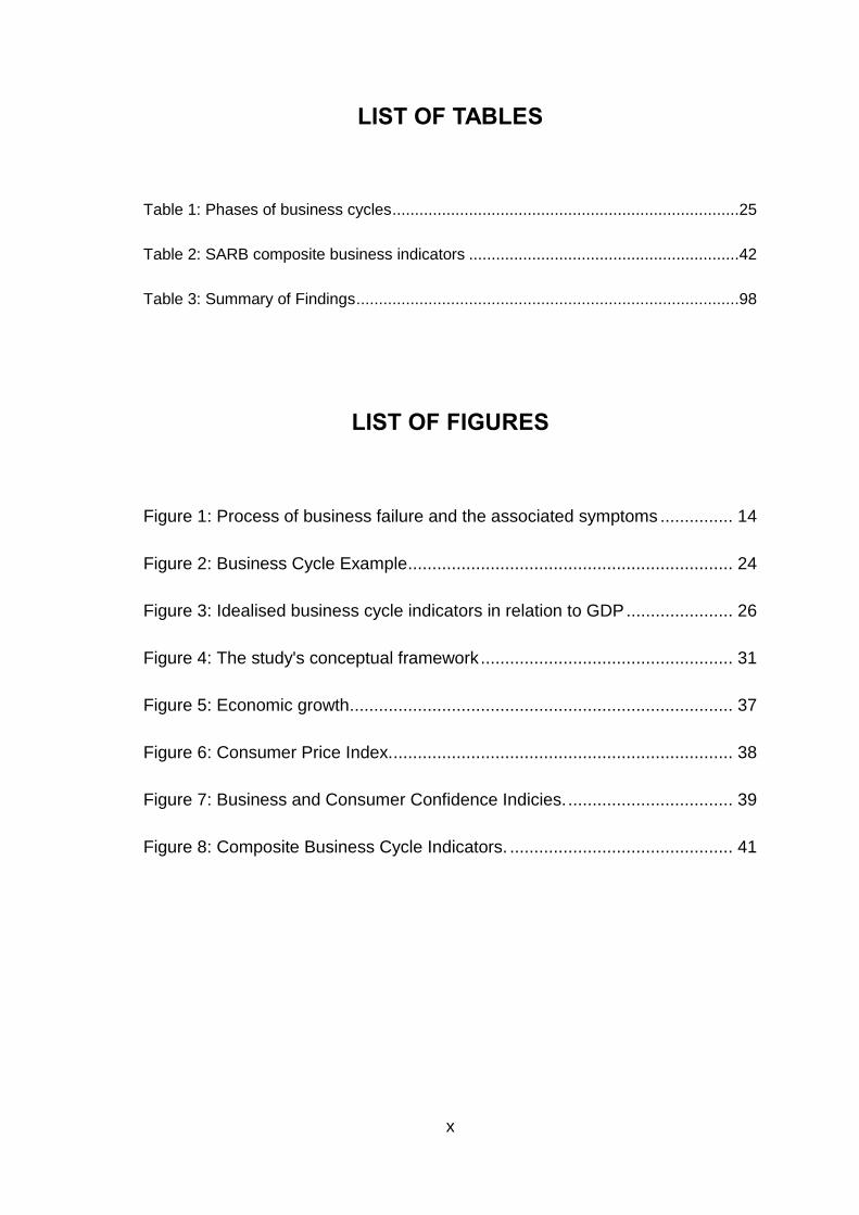
LIST OF TABLES
Table 1: Phases of business cycles .............................................................................25
Table 2: SARB composite business indicators ............................................................42
Table 3: Summary of Findings .....................................................................................98
LIST OF FIGURES
Figure 1: Process of business failure and the associated symptoms ............... 14
Figure 2: Business Cycle Example ................................................................... 24
Figure 3: Idealised business cycle indicators in relation to GDP ...................... 26
Figure 4: The study's conceptual framework .................................................... 31
Figure 5: Economic growth............................................................................... 37
Figure 6: Consumer Price Index. ...................................................................... 38
Figure 7: Business and Consumer Confidence Indicies. .................................. 39
Figure 8: Composite Business Cycle Indicators. .............................................. 41
xi
LIST OF ACRONYMS AND DEFINITIONS
BCI – RMB/BER Business confidence index
BER – Bureau of Economic Research
CCI – FNB/BER Consumer confidence index
CPI – Consumer price index
GDP – Gross domestic product
OECD -Organisation for economic cooperation and development
StatsSA – Statistics South Africa
1
1 CHAPTER 1: INTRODUCTION
1.1 Introduction
The privately owned business sector is a very complex environment, which is
characterised by a great variety of influencing factors emanating from within the
business (e.g. management, nature of business, etc.). According to
Bhattacharjee, Higson, Holly, and Kattuman (2009) nearly 50% to 90% of new
businesses end up failing as a result of micro and macroeconomic factors in the
business environment. The firms’ exits or bankruptcies are regarded as unlikely
situations in the process of continuous corporate growth and development.
Bhattacharjee et al. (2009) point out that firm exits are deemed to be cyclical in
nature. Exits due to bankruptcies are often associated with bad economic times
(the economic downturns), and acquisitions are often associated with
recoveries. Presently, a lot of literature has focused on different aspects relating
to business exits by concentrating mainly on endogenous factors as opposed to
the influences of the macroeconomic factors (Balcaen & Ooghe, 2006;
Bhattacharjee et al., 2009)
Despite the increasing knowledge about the influence of macroeconomic factors
on business continuance, there is little research that investigates these effects.
For instance, there is limited published research about investigating the impacts
of macroeconomic instabilities on the propensity of firms to exit, or about the
correlation between bankruptcy and acquisition and firms' exit. In this regard,
various analyses have focused on single impact factors such as bankruptcy or
acquisition and their influences on business exits (Chava & Jarrow, 2004;
Claessens & Klapper, 2002). In more cases, analyses of the impacts of the
macroeconomic factors have tended to focus primarily on the aggregate shocks
on the overall amount of a firm's formation or dissolution (Delli Gatti, Gallegati,
Giulioni, & Palestrini, 2003). The current research seeks to understand the
connection between business failure and the fluctuations in the macroeconomic
factors within the context of South African firms. The uniqueness of this study,
2
therefore, is derived from its ability to integrate various macroeconomic
influences on business continuance at a national level.
The business continuance in emerging economies such as South Africa is
influenced by serious macroeconomic issues since they depend largely on
external influences. For instance, the global financial crisis from 2007-2009
presented a lot of challenges, not only to the emerging economies but also to
the developed economies alike. In South Africa for instance, Redl (2015)
observes that the recession has been followed by long periods of increasing
output gaps raising the question of whether or not the potential growth rates
were lower than they were estimated originally. Moreover, South Africa, like
other emerging economies, is also affected by a slow recovery from the
financial recession. This scenario has been aggravated by slow resolutions to
curb the deficiencies of the euro areas (Redl, 2015). Long-term unemployment
has been associated with slow growths in the industrial and production sectors,
characterised by high rates of business failure.
Studies have indicated that there exists a correlation between firms' entries and
exits. However, the nature of the relationships tends to differ significantly across
the industries, as well as in ascending and descending phases of the
businesses (Bachmann, Elstner, & Sims, 2013). Empirical studies have pointed
to the relationships between the macro-environments and the performance of
firms. These studies maintain that the movements in the aggregate businesses
failure rates and business establishments tend to correspond to the changes
occurring in the macroeconomic situations in the respective regions (Bachmann
et al., 2013). The life cycle hypothesis described in Bachmann et al. (2013)
highlights that the exit rates for businesses often arise during the economic
downturns and the periods which follow them. The hypothesis further suggests
that both the growths rates of businesses and exits vary in size depending on
the financial stability of the firms and the nominal and real shocks occurring in
the markets.
3
1.2 Background of the study
The South African economy beat the global analysts' history in 2006 with the
Bureau of Economic Research (BER) second quarter of 2006 pointing to some
of the outstanding facts. These included a GDP growth averaging about 4.9%,
one of the fastest growth rates in the country since the short-lived spurt in 1984
(Haasje, 2006). During this time, the business cycle of the country was running
at a record length of 19 months (Haasje, 2006). For South Africa, a country that
has exhibited great positive growth potential over the past years, the post-
recession period has seen it undergo a series of productivity growth shambles.
For instance, 2010-2015 saw a considerable slowdown in economic growth of
the emerging regions, characterised by a commodity slump (Redl, 2015). South
Africa has not been an exception to these influences with the industrial
production falling considerably as the agricultural sector was inflicted with a
serious drought. Consumer demands registered anaemic performances during
this period, characterised by a low consumer index. Business confidence was
also depressed as a result of low consumer perceptions, high inflation rates,
and low employment rates. Consequently, business exits in the country,
especially in the private sector, have remained high during the period 2010-
2015 (Redl, 2015). The principal objective of this research study is to
investigate the connection between business failure in South Africa and the
fluctuations in macroeconomic conditions. The objective of the current research
resonates effectively with the currently observed scenario in the performance,
continuance, and exit of businesses in South Africa in light of the incumbent
macroeconomic factors.
1.3 The context of the problem
The primary concern of this research study is to identify the link between the
business failure and the fluctuations in macroeconomic conditions in South
Africa. In essence, the study seeks to understand the confluence, if any, in the
immediate and lagged correlations existing between the fluctuations of the
macroeconomic conditions and the failure of business enterprises, and if these
4
can be founded on the basis of explorative research. The private sector plays a
significant role in economic development and continuance in South Africa, just
as in other developing economies around the world. These, characterised by
continued entrepreneurial activities through business innovation and growth are
vital to creating employment opportunities for the people, enhancing consumer
spending and overall growth of the economy (Magruder, 2012). Over half of the
labour force is supported by the privately owned companies (Redl, 2015).
Owing to the important role that the private sector plays in developing every
economy of the world, the sector is critical for ensuring economic growth and
recovery. Studies have concentrated mainly on explaining why businesses fail
but not in understanding the influences of macroeconomic conditions on the
rates of such failure, despite the connection being suggested in the various
literatures. This study is, therefore, unique in its address to this distinct area of
concern to the business community and the development of every nation
around the world. The connectedness of the global economies makes it
possible for fluctuations in one region to bear significant influence on the
economies that depend directly or indirectly on the affected regions. Emerging
economies such as that of South Africa are affected largely by the international
economies, which directly impact its macroeconomic positioning. In this context,
the current study will measure some of the macroeconomic factors which are
directly influence the business continuance.
1.4 Statement of the problem
A great deal of exploratory research has focused on delineating the reasons
why businesses fail or exit from operations especially in economically volatile
countries such as South Africa. Emerging economies like South Africa are
highly sensitive to fluctuations in global economic conditions since they are
largely commodity-driven and market dependent (Mark & Sul, 2003). Growths
and stabilities in the international markets are associated with positive growths
of such economies, and the adversities experienced in the international
economies bear consequent side effects on the local economic performances
and thus business continuance.
5
1.4.1 Main problem
What is the relationship between business failure and the fluctuations in
macroeconomic environments in South Africa.
1.4.2 Sub Problem
Understanding the interconnectedness between macroeconomic variables and
how this interconnectedness can predict and cause future business failure.
1.5 Significance of the study
This study seeks to develop an elaborate understanding of the connection
between business failure and the fluctuations of the macroeconomic factors in
the context of South Africa. The quality and uniqueness of this research lies
solely on its ability to study unique characteristics of the business and economic
realm that has remained largely ignored in the literature. The economy of South
Africa is currently facing a lot of challenges including constrained consumers’
ability to spend, high-interest rates, high taxation rates, falling per capita
incomes, increased indebtedness, and notable credit extensions at the
household levels, etc. These conditions are negatively suppressing GDP
growths as consumer confidence continues to drop. In South Africa, household
consumer index (HCI) accounts for 61% of the total GDP growth (Magruder,
2012). The collapse of consumers’ confidence levels does not bode well for the
country’s GDP growth. The findings of this study will, therefore, be very
instrumental in the following perspectives:
- The findings of this study will help to understand the role that fluctuations
in the macroeconomic environments play in exacerbating business
discontinuance or continuance in South Africa for prosperous decision
making in the production sector.
- The outcomes of this study will be useful for the industry in helping to
understand market timings for entry by delineating different
macroeconomic factors and connecting these with business failures.
6
Such understanding would help to reduce the rates of discontinuance
through correct positioning of businesses.
- The findings of this study would also be useful in comprehending the kind
of pressures businesses face depending on where the business cycles
lie within the macroeconomic environment.
1.6 Delimitations of the study
This study will focus solely on privately-owned businesses operating their
business operations in South Africa. The assessments on macroeconomic
factors will be based on the South African GDP, CPI, Composite Lead,
Coincident, Lagged Business Cycles, Business Confidence Index, and
Consumer Confidence Index. Other factors besides these, including the legal
and regulatory frameworks, will not be considered in this research.
1.7 Definition of terms
1.7.1 South African companies
This research focuses primarily on privately-owned business entities. These
entities will consist of companies (PTY) and closed corporations (cc’s) as
defined by the Companies and Intellectual Property Commission.
1.7.2 Macroeconomics
The macroeconomic factors refer to the economic factors which influence the
national economy in its entirety and show predictable patterns and the trends in
influencing one another to contribute to the overall development of the nation’s
production entities.
7
1.7.3 GDP (Gross Domestic Product)
The GDP is a macroeconomic factor that measures the national economic
conditions in a quantitative manner. It is a quantitative measure of all finished
goods and services produced within the borders of a nation at a specific time.
The GDP is defined as the total of a country's consumption levels, government
expenditure, investments, and exports less the imports.
(GDP = Consumption levels + Government Expenditure +Investment + Export –
Imports)
1.7.4 CPI (Consumer Price Index)
The CPI is a measure of the weighted average of the prices of consumer goods
and services including transportation, medical care, foods, etc. The CPI is
determined by averaging the price changes in each item.
1.7.5 BCI (Business Confidence Index)
The business confidence index is determined through the assessment of
production trends, orders, stocks, the current expectations, and the immediate
future of the business scenario. The BER BCI is the unweighted mean of five
sectorial indices: manufacturing, building and constructions, retail, wholesale,
and the new vehicle dealers. The BCI is gauged on a scale of 0 – 100 with 0
indices indicating a total lack of confidence and 100 full confidence in the
business scenario in the respective places.
1.7.6 CCI (Consumer Confidence Index)
The parameter measures consumers’ level of confidence and is disaggregated
by the income levels of the consumers, population groups, the administrative
boundaries (province), and Living Standards Measure (LSM). It measures the
degree to which consumers are optimistic about the status of their economy as
expressed in savings and spending levels. This study will base its
considerations of CCI on the BER definition which combines the results of three
8
measurements: the expected economic performance, the expected financial
positioning of the households, and the ratings of the appropriateness of the
present times to buy various durable goods.
Based on the BER determinations, the CCI is calculated as a percentage of the
total respondents expecting improvements in the future (the good time to make
a purchase for durable goods), less the percentage of the consumers expecting
the deterioration of the economic times (the bad times to buy durable goods).
1.7.7 Composite Business Cycle Indicators
The Composite Business Cycle indicators consist of leading, coincident and
lagging refer to the indices that are created by the South African Reserve Bank
(SARB) Board Conference to help in forecasting the changes in the direction
and shifts in the country’s overall economy.
1.7.8 Business Failure
Business failure is a common occurrence in today's business world with
competition rising from time to time and the factors influencing business
continuance becoming more complex over time. This aspect of business failure
is not as simple to define as it is to understand. A wide array of definitions has
been provided to illustrate the meaning and inferences of the term “business
failure” from different perspectives, depending on the incumbent factors
resulting in the failure. In literature, one or several dimensions related to
business failures, notably, the aspects of bankruptcy, closure, acquisition, and
the failure to meet the desired expectations, have been attributed to business
failure (Dias & Teixeira, 2014). Dias and Teixeira (2014) in their attempt to
define business failure, observe that the same occurs when a business closes
down its operations due to either financial reasons or the owners giving
preference to another kind of business. Moreover, business failure can also be
defined as a scenario in which a business closes down because it fails to meet
the required expectations, such as poor performance, little growth, low returns
on the investments, etc. A business may also fail due to personal or familial
9
reasons, such as relocation, retirement, etc., thus prompting closure or
dissolution.
This study adopts the definition of business failure provided by Pretorius (2009)
who observes that business failure is a process which occurs in three different
stages: the pre-failure stage, the failure stage, and the post-failure stage. Each
of the phases mentioned portrays unique characteristics which jointly contribute
to the overall failure. According to Pretorius (2009), a business failure emerges
from business decline, which is characterised by worsening performance in
consecutive periods and is associated with the distress in continuing operations.
The failure occurs when it is incapable of attracting new debts or equity funding
to reverse the continued decline. Under such conditions, the business is
incapable of continuing its operations under its current management or
ownership. Failure, therefore, is observed as the endpoint in the discontinuance
or bankruptcy. When failure is reached, the operations cease to take effect, and
the judicial proceedings often begin.
1.7.9 Business Cycles
Business cycles are a core concern of today’s research and economic watch for
the success of the global economy and local economies at large. Business
cycles are an important aspect worth understanding in this research due to the
critical role that they play in determining the development prospects and
downfalls at different times in different regions of the world. The term ‘business
cycles,' as the name suggests, describes the constant downwards and upwards
movement of a country’s or region’s gross domestic products within and around
its long-term trends of growth (Diebold & Rudebusch, 1996). The length of a
business cycle is measured by determining a full phase of a single economic
boom and a contraction within a single following sequence. A full phase of a
business cycle is characterised by three main sub-phases: a period of rapid
economic growth (also referred to as economic expansion), a period of
economic stagnation, and a period of economic contraction.
10
Due to the constant focus on economic growths and underdevelopment,
business cycles have also been considered as economic cycles. Zarnowitz
(1992) defines a business cycle on two main features. First are the co-
movements in the economic variables, taking into account the possible lags and
leads in the timings in economic developments. In this feature, Zarnowitz (1992)
considered the historical concordances based on hundreds of series, which
include the measuring of commodity outputs, the income levels of the
population, the interest rates, and amount of banking transactions, as well as
the transportation services. The second feature in the definition involves
dividing the business cycle into different divisions based on the contractions and
expansions in the economic conditions of the GDP growths. The latest business
cycle was marked by the great economic recession of the 2007-2009 financial
crises that affected economies across the globe affected all nations of the
world.
1.8 Assumptions
This study will be based on the following assumptions:
- That the secondary information referenced disclosed accurate and
correct information regarding the reasons for business closure.
- The statistical analyses presented in the secondary reports which
informed the consent of this report are correct and depict the correct
position of the said scenarios within the context of South Africa.
- The information on deregistered businesses is assumed in this study to
be correct regarding deregistration dates.
11
2 CHAPTER 2: LITERATURE REVIEW
The private sector performs a critical role in spurring development of the
economies of the world through entrepreneurial activities and intersectoral
growths aided by technology and innovation (Mark & Sul, 2003). Emerging
economies that are commodity-driven, such as South Africa, are very sensitive
to external influences through the actions of macroeconomic factors given that
they have a global presence. In such cases, the impacts of macroeconomic
factors are experienced in all production and distribution sectors of the economy
(Ambler, Cardia, & Zimmermann, 2004). For firms to grow and continue
operating in a profitable manner, they must measure, document, and predict the
occurrences of various macroeconomic cycles and their influences on
production and distribution channels to ensure sustainability of production. This
study, therefore, explores the influences of fluctuations in different types of
macroeconomic factors on business failure in South Africa.
2.1 Introduction
This section of the study provides an illustrative review of the literature focusing
on the core concerns of the study’s objectives from the research perspective.
The review process commences with the understanding of business failure from
the perspective of the available literature and how this is influenced by various
macroeconomic factors. This section then draws a distinct conclusion on the
position of the literature concerning the objectives of this study.
2.2 Business Failure
Business failure is a broad concept which has dominated the literature in the
recent past due to the increasing business competition and complexities in the
business environment. The definition of business failure, despite a widened
focus it has received in the past, has varied within the available literature.
Commonly, business failure is defined in the literature by two main tenets:
bankruptcy and acquisition. For this study we will be focusing on business
12
failures only. Business failure can occur overnight as has been witnessed in
numerous cases (Pretorius, 2009). The factors that result in business failures
emanate both from within the business entities and from the macroeconomic
environments in which they operate. While the internal (micro-factors) are easily
controllable through the change of management, organisational restructuring,
and redesign, the macroeconomic factors are beyond the firms' controls. Due to
these changes, it is essential that the firms adjust their forecasts and operations
to go through and overcome the anticipated fluctuations in the macroeconomic
conditions.
In another sense, He and Kamath (2006) approach the concept of business
failure from a generic point of view, illustrating that failure occurs after decline
and cessation of business activities in the firm. The generic nature of these
definitions further suggests that the time of entry to the business is essential in
determining the impacts of the macroeconomic factors on the future operations.
The generic definition of ‘business failure' can be applied comfortably to South
Africa, and one can try to tie these to the understanding of South African
researchers from the local perspectives. From the generic point of view, we
notice that the macroeconomic fluctuations of the developed and the developing
nations' economies on the South African businesses influence whether or not a
firm in the region falls within the generic definition of ‘failure.' This observation
tends to support researchers’ view that the late entry of South African
businesses into the entrepreneurship field may be the main impact on rapid
discontinuance of businesses in South Africa.
2.3 The theoretical underpinnings of Business Failure
According to Aldrich and Martinez (2007), theory is an important aspect in
providing an interpretive lens for understanding every phenomenon of business
failure. This opinion is further supported by Hair, Black, Babin, Anderson, and
Tatham (2006) observe that theory provides a systematic, consistent and
comprehensive explanation to various phenomena of interest to the analysts.
Since the objective of this study is to determine the influence of macroeconomic
factors on the failure of businesses, the correlation between the two variables
13
can be unveiled theoretically; an analysis of the cause of the failure helps
promote an understanding of the failure’s occurrence. Specifically, explanatory
theories can be utilized to connect causes of the events leading to business
failures.
Aldrich and Martinez (2007), from a theoretical perspective, concluded that
following the rules and principles of business management are an essential
aspect of ensuring the success of businesses. This indicates that the firms must
comply with the impending rules of businesses, lest they risk being closing
operation. This explanation underpins research of Hair et al. (2006) and their
assertions on the principle of competition and adaptation in the business
environment. Based on these observations, businesses’ continuation is
comprehended from the perspective of Darwinian Theory of survival of the
fittest. In this respect, for the businesses to survive and become more
competitive, they must continuously adapt to impending environments. Part of
the adjustment/adaptation is to embrace the emerging competitive variations
due to changes occurring in society and the business society as a whole
(Aldrich & Martinez, 2007). Based on these observations, it is evident that
understanding the nature of competition in any area of production is akin to
understanding the ways of ensuring effective survival in the highly competitive
business environment. The rule of strategic management is an essential
component of ensuring the continuation of businesses in every scenario. The
concept of strategic management is to develop clear strategies suitable for
overcoming every possible obstacle.
2.4 The symptoms of Business Failure
There is no consensus in the literature as to how business failures occur, nor is
there a definite point in time when a firm is declared failed (closed down).
However, there are various signals that describe warning signs for the failure of
businesses. For instance, He and Kamath (2006) described a series of stages
which indicate the warning signs and symptoms of a failing business enterprise.
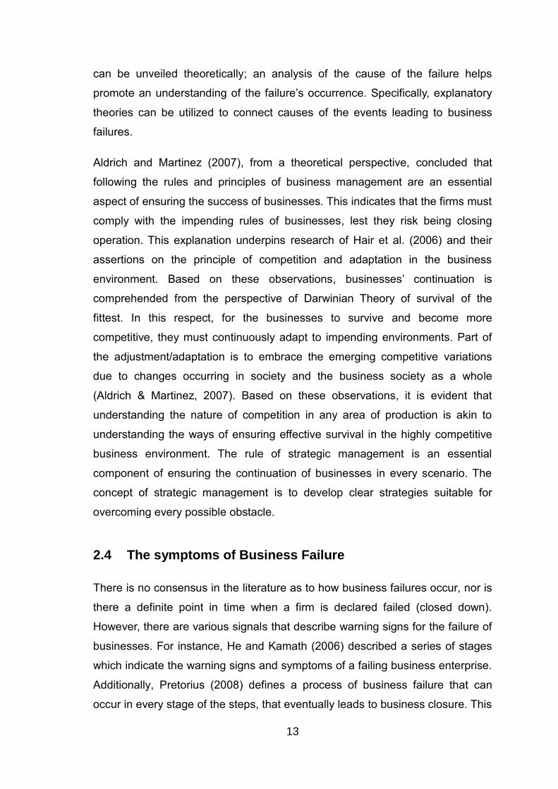
Additionally, Pretorius (2008) defines a process of business failure that can
occur in every stage of the steps, that eventually leads to business closure. This
14
individual step identifies the negative consequences and highlights the impact
they have on the survival of businesses. Evidently, most of the symptomatic
expressions signaling the onset of failure for businesses occur at the distress
and crisis stages. (The distress stage is associated with the firm’s inability to
meet their present financial needs without having to borrow from other
businesses or banks).
Figure 1: Process of business failure and the associated
symptoms (Pretorius, 2008)
According to Honjo (2000), there exists a close relationship between the returns
accrued from the business and the risks of its consequent operations. For these
reasons, a primary determinant of the risks is the dwindling profitability of the
firms. Low profitability conditions make it rather hard for the businesses to meet
their current needs. Due to these, businesses resort to either borrowing or
dipping into the financial reserves, thereby weakening their financial position for
any unexpected need. When firms are incapable of meeting their current
financial obligations, a crisis occurs. These two related stages (distress and
crisis stages) are therefore key indicators of failing businesses.
15
2.5 Causes of Business Failure
2.5.1 Endogenous Causes
Endogenous factors relate to those that emanate from within the business
environment. Various studies have investigated the correlation between various
endogenous factors and the concept of failure of businesses. The most
prominent issues relate to management practices and the financial conditions of
the firms. Based on the Salman, Fuchs, and Zampatti (2015) study, these
issues can be classified into two categories: management-related factors and
financial-related factors. The most common endogenous factor that results in
the failure of firms is poor management practices. Management practices, and
especially management styles, are key to designing a suitable path for
businesses to exist and operate with certainty, and thus ascertain the success
of the respective firms in competitive environments.
According to Salman et al. (2015), the success of any management system is a
definition of the ethical principles that govern business operations within the
firm. Lack of proper ethical entrenchment, therefore, constitutes poor
management and can easily result in failure of the businesses. Well-known
examples that illustrate poor leadership and a lack of ethical management are
Enron and Satyam. In other cases, the financial positioning of companies has
also been associated with business failure. However, Everett and Watson
(1998) attach the financial component more to exogenic factors than to
endogenic contributions since the financial stability of a firm is determined
primarily by their profitability, which, in turn, is a factor of various externalities as
well.
a. Management related factors resulting to Business
Failure
The management practices adopted by any company’s executive are the most
common causes of failure or success of the business. In this section, literature
has been analysed and presented with various scenarios, where poor
16
management practices have continued to lead to business failure. The most
recent of these cases are Enron and Satyam, among others. A diversified
content has focused on the contributions of management failures towards
business failure to put the arguments into the perspective of this research
(Altman, 1983; Balcaen & Ooghe, 2006; He & Kamath, 2006; Liu, 2004;
Pretorius, 2009).
Lukason and Hoffman (2015) classify business failures into three categories of
management-related factors: the voluntary internal actions undertaken by the
management; the influences of the deterministic management environments;
and the integrative factor between the two factors. In examining the prevalence
of these factors towards contributing to business failure, the researchers
concluded that the influence of internal decisions in contributing to the business
failure is more rampant compared to the deterministic environmental factors of
the integrative factors. Their study attributes the high prominence of
voluntaristic factors causing business failure to various intuitional and approved
theoretical underpinnings. These include the groupthink theory, the curse of
success theory, the threat-rigidity theory, and the upper echelons theory, all
competing in almost equal proportions to explain the reasons for failure. For this
study, the voluntarist theories seem more relevant in explaining the causes of
business failure in South Africa.
The voluntarist theories maintain that the decisions which result in business
failure are voluntarily made by the management, highlighting the need to
understand within which process step of failure the business is in (Pretorius,
2008). According to Dubrovski (2009), wrongful decision-making is an essential
explanation of businesses failing to continue. Some of the most commonly
referred to and analysed voluntarist theories include the echelons theory and
the threat-rigidity effect theory. Both theories concur that voluntary decisions
made by management are the primary causes of failure of businesses. The
theories are based on the observation that a lot of failures that occur in the
business field are a result of the business owners/managers making poor
decisions regarding the manner in which they run and operate their businesses.
Consequently, poor management choices lead to discontinuance, if proper
17
intervention mechanisms are not put in place in time to reverse the effects. The
preferred strategic management sources would favor continuance over
discontinuance of businesses since they tend to reflect how the management
perceives the progress of their businesses at various times. These include the
decision-making process and how they are achieved within the context of the
businesses.
b. Comparing small and large firms Business Failure
Comparing small firms and large firms in terms of flexibility in decision-making
and the contributions of these to the business continuance, Franco and Haase
(2009) maintain that small businesses are well-placed when it comes to
decision-making and flexibility. As a result, they can correct all the wrongs in
time to save the company, before grievous effects mar their business
successes. The study attributes such high flexibility to the simple ownership and
management structures that allow quick decision-making. For instance, the
researchers notice that a majority of small-scale businesses are owned and
managed by an individual, a small group of owners or, on most occasions,
families. This makes it easy for the top managements to consult quickly to
enable quick, easy, and effective decisions considered healthier to the life of the
businesses. On the other hand, the decision-making processes in large
companies are often slow and procedural. These procedural processes tend to
delay decision-making processes. The ease in decision-making is determined
basically by the levels of management involved, the number of people involved,
and the chartered procedures that the firms consider necessary for decision-
making. Particularly, the processes of collecting and disseminating the decision
information from and to the concerned persons and the overall time involved
inhibit quick responses to adverse conditions such as the presence of a crisis.
These slow responses tend to exacerbate the negative effects, due to delayed
handling of the eminent adversities. This observation by Franco and Haase
(2009) resonates with Dubrovski (2009) who believes that in the event of a
crisis within the business, a quick response is often necessary. Delaying such
actions would result in worsening the adverse conditions (Pretorius, 2008).
18
2.5.2 Exogenous factors
The onus of this research is to investigate the effects of macroeconomic factors
(exogenous factors) on business failure. Exogenous factors are those factors
that emanate from outside the business environment, and which are beyond the
firms' control. They are comprised of macroeconomic factors, such as the
inflation rate, the consumer confidence index, the consumer perception index,
the GDP growth rate, and trade connections with external partners like supply
chain orientations, the market prospects, etc. These factors are discussed in
section 2.3 on the influence of macroeconomic factors on business failure.
2.6 Macroeconomic effects on Business Failure
Several macroeconomic factors have been associated with business failure in
various literature findings. This section reviews some of these associations from
the perspective of the existing research. One of the landmark studies in this
aspect is reported by Bhattacharjee et al. (2009). The study investigated
macroeconomic instability as the key determinants of business exit (bankruptcy
and acquisition) in firms in the UK. Specifically, the study investigated how
macroeconomic conditions in the UK influenced the firms' bankruptcy and
acquisition. The study established that the macroeconomic instability bears an
adverse effect on business hazards such as bankruptcy and acquisition.
Particularly, macroeconomic instability was found to escalate the hazards
related to bankruptcy and lowered the possibilities of acquisition due to weak
operational and financial power of the associated firms. Also, the study
established that the macroeconomic factors in partnering countries, such as the
US also bore direct negative impacts on the bankruptcy of UK firms (despite
bankruptcy hazards of these firms being counter-cyclical). Macroeconomic
instabilities in the US were in fact found to be better predictors of acquisition
hazards of UK firms (despite the acquisition hazards of UK firms being pro-
cyclical in nature).
Again, these findings reflect those of Redl (2015) who suggested that the
interconnectedness between world market economies have a direct impact on
19
each other. For instance, South Africa's firms trade much with Africa, Europe,
and the United States. As a result, macroeconomic instabilities of these
economies bear a significant impact on the operations of the firms at the local
level. The poor business performance and eventual exit of many firms in South
Africa, documented in Redl (2015), is a clear indication of such instabilities
affecting business continuance in the region. The USD and the GBP, which are
regarded as the world's strongest currencies and the most common units of
trade and exchange, are affected by such instabilities, and will in turn affect
international economies in terms of currency stabilities. Therefore, they bear
direct negative consequences on South African firms (Smit, Frankel, &
Sturzenegger, 2006). In related research, Liu (2004) assessed whether
macroeconomic factors, including credit conditions, profitability of firms,
inflation, etc., influenced the observed fluctuations in business failure among UK
firms for the period 1966-2003 using a VECM approach. The findings
established that the firms' entry times, access to credit, profit conditions, and
inflation in the UK influenced business failures. The study also found that
deregulation policies established by the government of Margaret Thatcher
altered the relationship between the failure rates of the firms and the impending
macroeconomic indicators’ values during the same period. These findings
further point to study by Redl (2015), Smit et al. (2006), about
interconnectedness of different sectors of the economies around the world.
The last century has seen an intensive expansion of the global economies as
the world becomes more connected and markets expand. As these economies
grow, more products continue to rise, and firms realise the importance of their
ability to thrive and satisfy rising global demands. Due to the demand for trade
between economies, the global trade policies developed by a country and the
attitudes towards establishing new businesses and making them thrive are
intricately connected to the macro and microeconomic scales. Khader, Rajan,
and Sen (2014) examined the effects of various macroeconomic factors that
influenced the ease of doing businesses across different countries. Their study
indicated that the various macroeconomic factors, such as lending rates, access
to the internet and its safe use to spur development, and the growth rates in the
GDPs had a direct and significant impact on the survival of businesses. In a
20
similar way, it is agreed that liquidity constraints in each economy are essential
macroeconomic factors determined by GDP growths and that they bear
significant influence on business successes. Fairlie and Krashinsky (2012)
observed that a greater asset base is often associated with increased rates of
business entry. Consequently, the sustainability of these businesses is
determined primarily by the country’s GDP growth prospects, inflationary
conditions, consumer purchase capacities, and the interconnectedness of
different markets.
It is evident that macroeconomic factors, macroeconomic conditions,
adaptation, and forecasts about economic dynamics influence business
continuance and business failures. Hence, the following sub-sections highlight
specific macroeconomic factors and how they impact businesses.
2.7 Economic performance of the country
Economic recessions present some of the most unpredictable events in the life
of a business; they need to be monitored in order to effectively determine the
success and continuance of businesses. Fluctuations of the economic
performances of counties are characterised by peaks and troughs. The trough
represents bad economic times while the peaks signal good fortune in terms of
economic growth during certain times of its existence. Economic insolvencies
are capable of causing declines/discontinuance of businesses, if not handled
carefully. Sudden declines in the economic performance at the international or
national level bear significant impacts on the performance of businesses (Liu,
2009). For instance, declines in economic performances are consequential in
influencing the declines in particular activities conducted by organisations.
Consequently, declines in business activities result in declines in returns and
may easily lead to insolvency of the businesses (Liu, 2009).
Regarding the changes in economic performance regionally, nationally or
internationally, Everett and Watson (1998) looked at the influence of changes in
clients' purchasing trends on a company's performances from time to time.
Specifically, the study focused on the impacts of declines in the purchasing
21
power of a country as results of hard economic times (recessions) and their
impact on the business continuance. The study found that declining purchasing
power (associated with the CPI) affects the performance of the businesses
negatively, and consequently, the failure of the businesses. Declining
consumption patterns can be alleviated by working out strategies to improve the
customers’ perception about the products. Some of the adjustment practices
that Lukason and Hoffman (2015) recommend include improving the marketing
practices, price modeling strategies and branding in distinct markets among
other relevant strategies. The study, which covered a total of 50 medium scale
enterprises, found that the changes in consumers’ buying patterns are
influenced by a series of events, including the socio-political occurrences at the
local and international levels. Accordingly, Everett and Watson (1998)
concluded that adapting to the external political and social conditions in the
environments in which the respective businesses operate is an essential aspect
of ensuring sustainability of the businesses in the long run.
Competition with other big companies, e.g. multinationals, is another important
aspect that contributes to recessions in business performance over time. A
business recession is characterised by poor performance (low returns from
sales of products and services rendered). These factors impact the quality of
businesses by deteriorating financial stabilities (De Loecker & Van Biesebroeck,
2016). Unbalanced competition with businesses from highly established
regions/developed regions tends to impact local businesses adversely. For
instance, the entry of large multinational companies into local markets, aided by
free trade, may bear consequential impacts on the price conditions and
fluctuations in local markets. The large companies are capable of segmenting
local markets by using them as dumping sites for their products. As De Loecker
and Van Biesebroeck (2016) highlight, most of these large companies produce
at cheaper prices and subsidized costs compared to local small or medium
enterprises, thereby pushing smaller local enterprises out of businesses.
In an example to justify the influence of free trade on the development of
businesses in the developing countries, Shaw, Cooper, and Antkiewicz (2007)
used the scenario of Asian multinationals in local economies and their
22
competitive effects on local African business ventures. A lot of the Asian
multinationals (e.g. Japanese, Taiwanese, Chinese or Indian multinational
companies) dump their products, (e.g. assembled motor vehicles) in African
markets at cheaper prices than the locally assembled ones. This makes it hard
for African companies to sell their products locally. If such unbalanced
competition is not strictly supervised, local businesses may find it too difficult to
cope with the competition and eventually discontinue their businesses due to
the inability to compete. To regulate such competition and enhance the growth
of local companies, the governmental trade policies are essential. Shaw et al.
(2007) recommend implementing regulatory measures for the entry and
operation of foreign companies in local markets, such as increasing taxes for
foreign companies selling their products in local markets, so that they can sell at
relatively fair prices.
2.8 Business Cycles
It is observed that under capitalist economies, the aggregate economic
variables undergo constant trending fluctuations, which tend to depict almost
the same characteristics. These anomalies posed major challenges to
economists in ancient times and formed the basis for economic analyses.
Following the development of Keynes's General Theory, economists came
forward to develop an illustration for this challenging anomaly, leading to the
development of the business cycle theory (Mankiw, 1989). Under normal
circumstances, a cycle describes recurrent phases of the same complete event
at different times under different influencing conditions.
In the last few decades, the concept of business cycles has attracted the
attention of economists and researchers around the globe. Since the pioneering
works of Burns and Mitchell (1946), a lot of attention has been paid to business
cycles and the factors that influence them. Mainly, the connection between
business cycles and the macroeconomic influences has been the center of
focus in numerous studies conducted in the recent past. Due to the increasing
focus on this aspect, defining the concept of ‘business cycle’ has also been fluid
in the existing literature. This section discusses the influence of macroeconomic
23
factors on the business cycles around the globe. However, to understand the
connection between the two, it is essential to first define business cycle.
The concept of the business cycle has had various definitions in scholarly
literature. One of the earliest definitions of the concept was provided by Burns
and Mitchell (1946). They defined a business cycle as a series of fluctuations
evident in the aggregate economic activities of a nation, which are evident in the
nations’ organisation of its business activities. A complete cycle is made up of
various expansions occurring at almost the same time, and affects various
economic activities followed by a similar recession, contraction, and revival in
economic performance which merge up into the next expansion phase.
According to the definition, a full business cycle is comprised of two main
features. The first feature represents the co-movement within the economic
variables individually and takes into account the possible leads and lags in their
timings. The emphasis laid on the existence of a pattern in the co-movements
among the economic variables during the phases of the business cycle led to
the coinage of the composite leading, coincident and lagging indices by Shiskin
(1961) as measures for determining business growths at a macro-level.
The second significant feature in Burns and Mitchell (1946) definition of
business cycle is the division of the cycle into different phases, also referred to
as business regimes. In this approach, the analyses treated economic
expansions from the associated contractions. This notion of the cycle approves
the observation by Shiskin (1961) by maintaining that some series are
categorised as leading, while some others fall under the lagging indicators for
the different stages of the cycle. These phases are influenced greatly by the
overall state or conditions of the respective businesses. Apart from the post-
WWII economists, the latest economists have utilised these features immensely
in describing the economic conditions of different regions and their consequent
influences on business activities (growth and discontinuance).
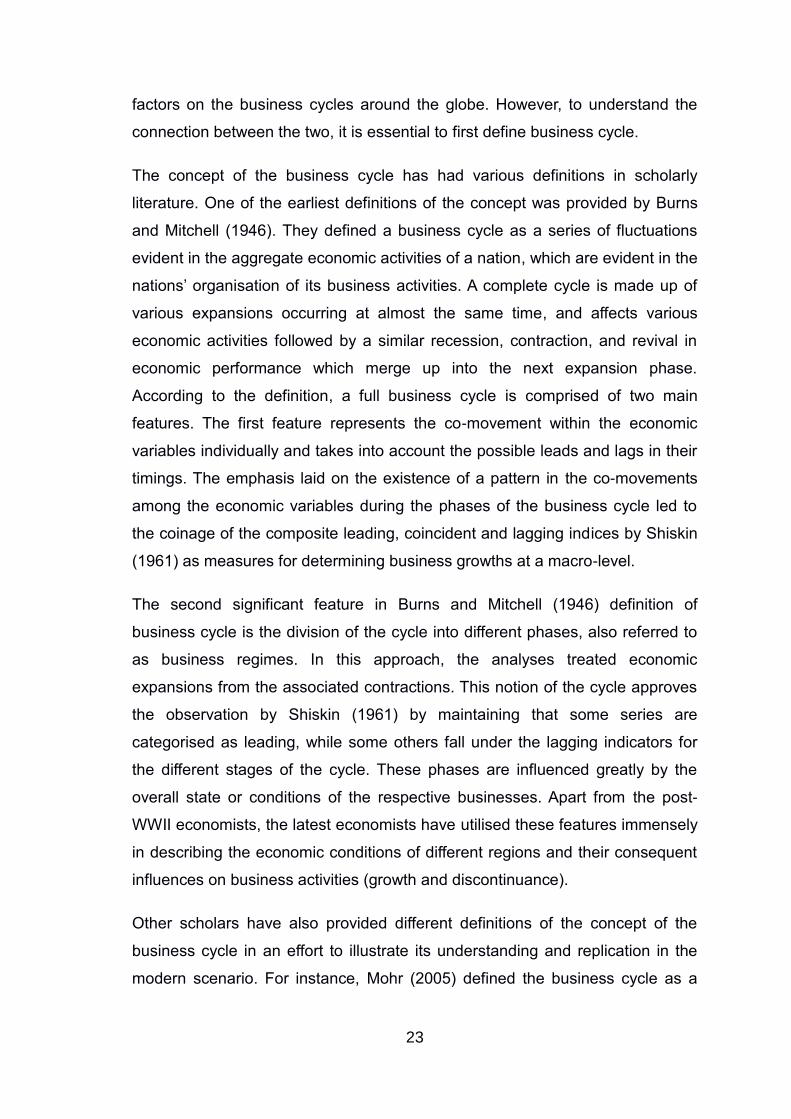
Other scholars have also provided different definitions of the concept of the
business cycle in an effort to illustrate its understanding and replication in the
modern scenario. For instance, Mohr (2005) defined the business cycle as a
24
series of patterns characterised by expansion and contraction of the aggregate
economic activity. A business cycle is measured by the real gross domestic
product. According to this definition, the growth phases (regarding leaps and
bounds) are clear indicators of the overall trends, which can be utilised in
determining the onset and cessation of different cycles. The sequences of
change (defining the phases of business cycles) are considered to be recurrent
in nature but are not periodic. Concerning duration of existence, or from one
cycle to another, the time varies significantly (one year, five years, ten years,
etc.). Each phase is divided into various shorter cycles with similar
characteristics or amplitudes of their approximations. This is because each
phase tends to portray similar patterns. Figure 2 shows the different expansion
and contraction phases of the business cycle from a theoretical perspective.
Figure 2: Business cycle example (Mohr, 2005)
From the observations in the diagram, a new business cycle begins at the
lowest GDP position characterised by low economic growths. At the end of the
trough growth, expansion is often characterised by a sustained increment in
economic activities until the expansion reaches the highest level of GDP growth
in that phase. This highest phase of the cycle is referred to as the peak and is
regarded as the third element of the business cycle. After the peak, the
economy begins to decline with economic activities shrinking from time to time.
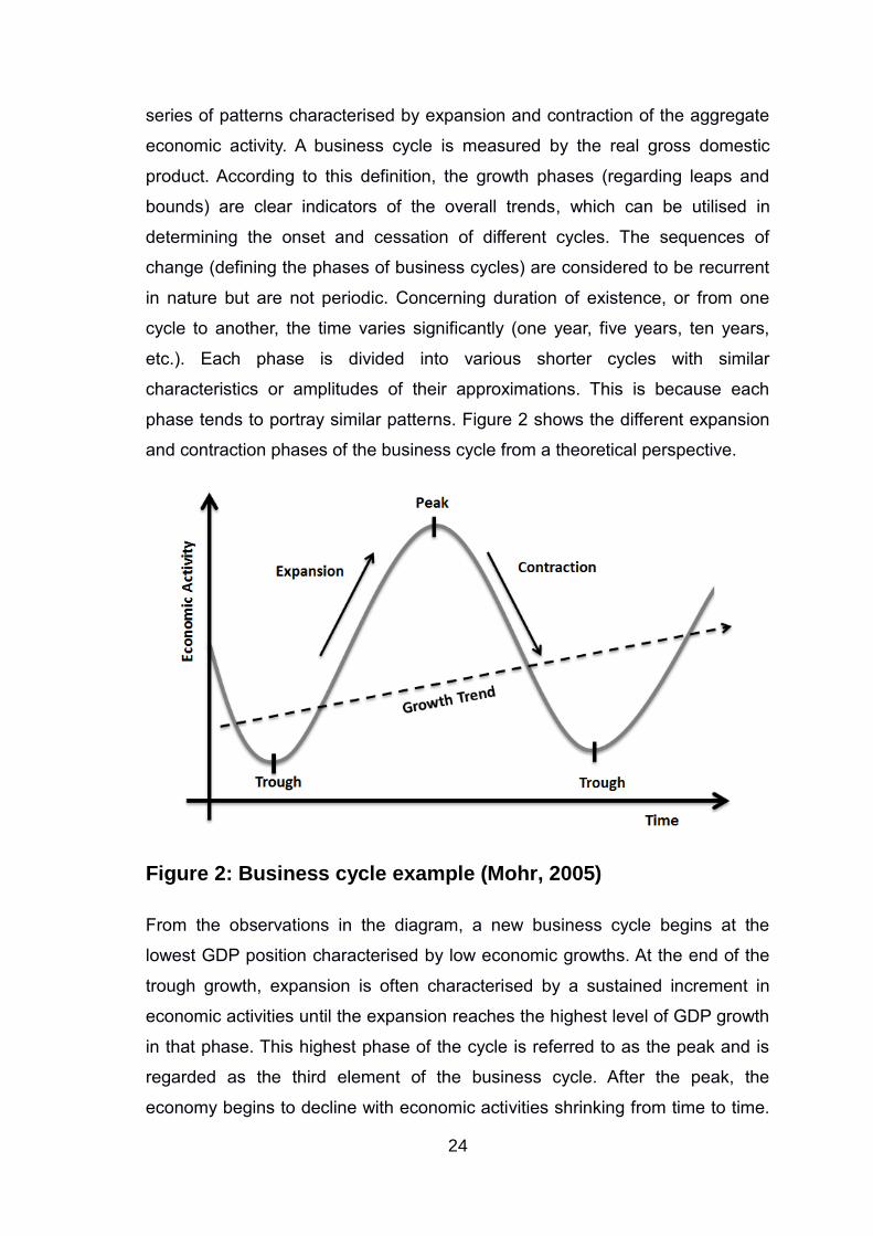
25
This is the decline stage characterised by a falling GDP and decreasing
economic activity. The decline is referred to as the GDP contraction and is the
last phase ensuring the beginning of a new cycle. The events characterised by
these phases are illustrated in Table 1.
Table 1: Phases of business cycles
Expansion Phase Peak Phase Contraction Phase Trough Phase
- Level of
economic
activities
increase
- More goods and
services are
realized
- Household
expenditure
levels increase
- Interest rate
decreases
- Inflation levels
increase
- The economy
consumes most
of the resources,
e.g. skilled labor
and capital
- There is an
upward pressure
on prices and
the balance on
the current
account worsens
as a result of
higher imports
- Level of economic
activity decreases
- Fewer goods and
services are
produced
- Spending begins
to decline
- Interest rates
begin to increase
- Inflation also
decrease
- Unemployment
rates increases
- Turning point is
realized at the end
of the contraction
phase
- Lower inflation rates
allow the central
banks to begin
lowering the interest
rates
- Current accounts
begin to improve
due to low costs of
exports and lack of
domestic demand
for imports
Keynes on the other hand, attributed the fluctuations in the economy to the
fluctuations in investment spending (Brue & Grant, 2012). This is because
investments bear a direct impact on the economic development of countries by
attracting income and exchange. According to the Keynesian view Mankiw
(1989) of business cycles and recessions, governments tend to take
extraordinary measures such as increasing money circulation, increasing
spending on investments, etc. to counter the adverse effects of the recessions
and create a multiplier effect to the economy at large. At inflation swings,
measures such as reduction in money supplies, contraction of spending and
rising of taxes are common practices to keep the economy stable and to steady
business performance.
26
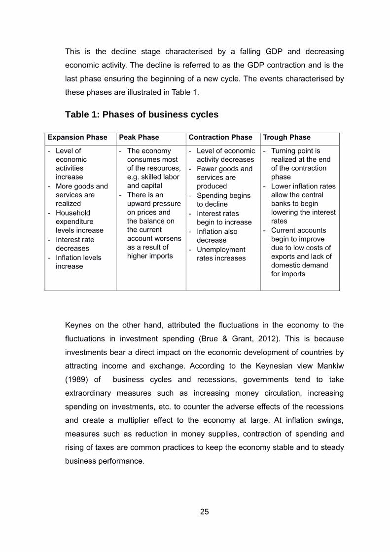
Composite leading, coincident and lagging indicators have been utilised in the
modern economic analysis scenario to predict and chart business cycles.
Figures 2 & 3 shows the relationship between GDP and the leading, coincident
and lagging indicators at different times of the business cycles.
Figure 3: Idealised business cycle indicators in relation to GDP
(Board, 2001)
2.8.1 Breaking down the Business Cycle
The economic environment of any country is a very complex aspect of analysis;
its correct delineation requires an absolute and comprehensive consideration of
various factors affecting economic growth. It includes all internal and external
factors that influence economic growth patterns at different times. The phase of
the cycles is an essential aspect for planning a firm’s productivity and growth.
Since the business cycles occur in stages, as illustrated by Diebold and
Rudebusch (1996), their onsets set an important platform for businesses to
brace for hard times. This way, peak economic times can be used by
companies to capitalise on their returns and compensate for any losses incurred
27
during the low economic growth phases. It is, therefore, important for traders to
analyse and interpret the cycle phases to aid in making correct decisions to
enhance their productivity.
Ideally, during the peak cycles, the economies exhibit positive growths
regarding the intensification of the economic activities, including improved
employment conditions, increased industrial productivity, low inflation rates,
improved sales and good income levels for individuals, countries, and regions.
During the low peaks, i.e. recessions, the economic growth is negative,
characterised by shrinking demand, and attenuation of economic conditions.
As Ambler et al. (2004) and Redl (2015) observe, in the present nested
economies, the cycles of major economies, such as those in the developed
world, affect the cycles in other regions that depend directly or indirectly on
them. Although the South African economy is currently classified under the
fastest growing economies of the world (the BRICS nations), its growth is
dependent to a large extent on the growth of other developed nations such as
the US, the UK, and China. For these reasons, to ensure stable and consistent
growth, the government of South Africa and the firms within must pay close
attention to the business cycles of other countries. This study analyses the
nature of business cycles within the context of theory and practical application
from the South African scenario to larger global contexts. The analyses are then
used to predict the future scenarios on the movement of business cycles in
South Africa.
2.8.2 Business Cycles and global Interconnectedness
The world is increasingly connected through technology, increased mobility of
people, goods and services, and political influences, and thus, there is
economic interdependence. Global interconnectedness is augmented primarily
by the expansions in technology and increasing demands for goods and
services in regions that lack the same. However, the mode of relationships and
dependence between countries and regions is imbalanced because of
dependence on growth rates, productivities, and economic conditions.
28
Developing countries and the least developed countries depend largely on the
developed economies for their continual growth, as with the case in South
Africa’s resource exports to developed economies (Ambler et al., 2004). The
flow of goods and services in different markets through trade is also significant
to the relational characteristics and dependence between different states in the
modern global economies. The developed countries, e.g. the United States,
European countries, China, etc., are often viewed as the economic hubs of the
world whose economic stabilities affect the other developing economies a great
deal.
2.8.3 The global business cycle and its changing dynamics
Empirical studies show that the rate at which the global economy is growing
presently is higher than it was about three decades ago (Stock & Watson,
2005). Historically, the world is in its fifth year of a string expansion since the
last depression of 2007-2009. Comparisons between the current and past
growth trends, however, reveal an inconsistent growth phase, which economists
describe as unusual. To put this into perspective, in the 1960s the GDP growth,
accounting for demographic shifts, was averaged at about 3.4%. This was 0.2%
higher than the averages of the growth experienced in the last decade. These
findings imply that just one feature of the current expansion is essential in
creating an imbalance in economic growth. However, Stock and Watson (2005)
observe that even though an expansion is evident presently, the length of the
present expansion is still far from reaching the historical highs experienced in
the past. Stock and Watson (2005) say that the present cycle is only half the
length of expansions registered in the 1980s and 1990s. This trend is clearly
evident in both the underdeveloped economies of Africa, the developing
economies of Asia and Latin America, and the developed economies of the
western countries. For instance, in the United States, the present cycle of
expansion is lower than the expansions recorded during the 1980s and 1990s.
Consequently, the same low expansion levels are evident in Europe’s major
economies, such as the United Kingdom, Germany, and France. The length of
Europe’s current expansion size seems to stack up against those registered
29
during the 1950s and 1960s which were longer than presently. These
observations are supported by the high growth trends in the region’s
economies.
According to Del Negro and Otrok (2008), a close comparison between the past
business cycles evident during the past centuries indicates a secular increment
in the lengths of the expansion periods and a decrease in the lengths of the
recession periods (the amount of times that the countries spend to go through
the full length of the recessions). In fact, the researchers observe that in the
more advanced economies, the stable economies of the developed countries’
recessions have disappeared since the end of the Second World War. However,
in the developing countries and other emerging markets, their long-term
development trends geared towards improving the dynamics of their business
cycles appears to be more mixed than smoothly trended as in the case with the
developed countries. Stock and Watson (2005) associated these observations
with the dynamics of growth factors influencing the economic developments of
these countries, as opposed to the more stable economies of the developed
nations.
Still, in regards to Asian countries, the current business cycle expansion has
recorded long-term trends in China and India, which are similar to the trends
observed in the Post-World War II scenarios recorded in the major European
economies, Japan, and other newly industrialised Asian economies. Increased
industrialization and of the Asian markets from oil and gas exports, and
diversification of the region’s economies, have seen them stabilising their cycles
over time. By stabilising the economies, de Haan, Inklaar, and Jong-A-Pin
(2008) observe that the governments of the above mentioned countries must
shield local production activities and the growth factors from external
interference (by foreign agents). The developed economies, such as the United
States, have protected their economy by restricting the goods sold in their local
markets from the outside, while maximising exports. In contrast, the developing
countries produce little for the foreign markets and thus import most goods,
making their economies susceptible to external interferences. Such
interferences destabilise the economic performance and development, hence,
30
the noted lack of consistency in the business cycles of these economies
compared to their developed counterparts.
The Latin American region, however, has shown opposite results regarding the
trends in its business cycles. For instance, the four largest economies of Latin
America, including Brazil, Mexico, Argentina, and Colombia, have failed to
record notable expansions in terms of duration since the 1970s when the region
recorded the longest expansion period. This lack of expansion is attributed to
the recurrent currency crisis in the region, which has resulted in economic and
trade imbalances. In the same manner, the share of the times which these
economies have spent in the recession periods has not declined notably since
the 1970s. These invariabilities in the expansion events in the developed and
the developing economies has been associated largely with the unstable global
economic conditions that show a lack of consistency and growth (Del Negro &
Otrok, 2008). These include unusual sustainable fiscal and external economic
imbalances, tightening monetary policies, rising inflation, cross-country inflation
spillovers, constant swings in the prices of commodity and assets, and related
financial squeezes.
2.9 Hypothesis statement
H1: Fluctuations in CPI causes business failure
H2: Fluctuations in GDP causes business failure
H3: Fluctuations in the Composite Leading Business Cycle index causes
business failure
H4: Fluctuations in the Composite Coincidence Business Cycle index causes
business failure
H5: Fluctuations in the Composite Lagging Business Cycle index causes
business failure
H6: Fluctuations in Business Confidence Index causes business failure
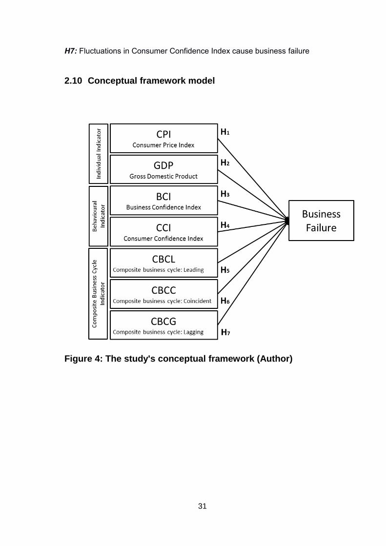
31
H7: Fluctuations in Consumer Confidence Index cause business failure
2.10 Conceptual framework model
Figure 4: The study's conceptual framework (Author)
32
3 CHAPTER 3: RESEARCH METHODOLOGY
3.1 Research Strategy and Design
The study adopts the cause-effect approach used commonly in exploratory
studies such as the current study. This has been enabled by restructuring the
research questions in the form of the hypothesis. Empirical evidence, which
illustrates cause and effect relationships and research analysis, will be
communicated from various published research studies. Data will be sourced
from macroeconomic databases that are published and where the data is
publicly available.
To understand cause and effect relationships and apply them quantitatively,
researchers in the social sciences have put forth some assumptions,
paradigms, and theories that underlie this study and its methodology. The
subsequent sections discuss epistemological and ontological paradigms,
approaches of positivism and interpretivism, and the need to form a basis for
these paradigms in order to proceed with the necessary research design.
3.1.1. Epistemology and ontology
3.1.1.1. Epistemology
Epistemology is the consideration of what constitutes knowledge within the
scientific and research realms. It is a paradigm of understanding the way we
know the truth about something and how we explain it (Collis & Hussey, 2013).
Owing to the fluidity in its definition, the term epistemology has been defined in
a varied manner in literature. For instance, Collis and Hussey (2013) describe
epistemology as the creation and dissemination of tenets of knowledge in
specific areas of scientific inquiries. In terms of the epistemological stance, the
researcher must consider the specific data or resources that describe the
required outcomes.
33
a. Data collection
This study will be represented using secondary data through the normal
process of data collection and analysis of facts. According to Collis and Hussey
(2013), objectivity in epistemological undertakings must be guaranteed by
ensuring that the data sets collected for use to justify the positions and facts
minimize bias. This can be achieved through the researcher's detachment from
the study in order to reduce personal influence. Consequently, accuracy and
soundness of the data used in this study will be of top priorities to the
researcher. It is essential that the data/information collected from the primary
sources is well-maintained and secure from any kind of interference, thus
guaranteeing the level of objectivity needed in the study. The soundness of the
data collected in this study, the data retrieved from the primary and secondary
sources will be used in their raw statuses without any form of modification or
prior processing. This will ensure that the results obtained are outstanding and
meet the standard ethical and objectivity conditions (Collis & Hussey, 2013).
Financially compiled secondary data will be used in this study, including
opinions from interviews and discussions, which are prone to personal biases
and interpretations. This said, business and consumer confidence indices are
measured through surveys of the respective sectors.
b. Data interpretation
There are two principles of data interpretation that are influenced by the level of
independence the researcher allows in his or her studies: positivism and
interpretivism approaches. Positivism, as a research philosophical stance, does
not include the opinions of the researcher interpreting the results of the study or
manipulating the data to derive the desired outcomes. The more the researcher
desists from injecting his or her opinions into the study outcomes, the more
objective the results will be. In the study, it is believed that by using quantitative
data on GDP, CCI, CPI, etc., the influence of the researcher will be eliminated
to make the findings sound, outstanding, and objective.
Further, the study adopts post-positivism as the preferred epistemological view
focused on understanding the connection between business failure in South
34
Africa and the impending macroeconomic factors. The CPI and GDP data will
be derived from real economic and financial information published on secondary
data, while CCI and BCI data will be surveyed and tested against the critical
and realistic philosophical basis.
A deductive quantitative approach will be used for this research based on
longitudinal secondary data. The data will be retrieved from accredited,
published, secondary sources to increase as much as possible the ensure
reliability and sustainability of results.
3.1.2 Ontology
Previously highlighted was the epistemological perspective that explained what
constitutes knowledge from an individual’s perspective in a particular field of
knowledge. On the other hand, the ontological perspective to knowledge
derivation explains the nature of the reality attained through the epistemological
explanations. However, far from the epistemological concerns, the ontological
approaches tend to raise the questions concerning assumptions made in
coming up with the suggested realms of knowledge explained and the
commitment that they hold to retain such views (Crotty, 2003). For any
particular view one holds concerning any perspective of knowledge, it is
imperative that a certain degree of assumptions needs to be made.
The two aspects of ontological perspectives described in this section will have
independent devotees to the operations and outcomes of this study. Key in
ontological perspective is objectivism, meaning various social entities exist in
their unique realities which are external to the social actors that govern their
existences. Second is the subjectivism aspect, meaning that social phenomena
are often created from personal opinions and perceptions and that the
consequent actions of these social phenomena (actors) prove their existences
(Crotty, 2003).
The current study adopts the ontology of the social world of meanings and the
ontology of the realistic world. In the first ontological assumption, the study is
developed on the assumption that the world being investigated is made up of
35
humans with different thoughts, opinions, and interpretations of various issues
happening around them. This ontological perspective is clearly demonstrated in
the choice for the use of different research methods for data collection and
manipulation approaches (The methods are described in the subsequent
sections of the study). These include data on macroeconomic factors such as
GDP growth patterns, etc. and the number of failed businesses within the
selected periods analysed through various statistical approaches to derive the
connection between the two sets. The composite business cycles, leading,
coincident and lagging, will provide the opinion-based interpretation of the
South African Federal Reserve Bank concerning the factors influencing the
ease of doing businesses in the region, as well as the macroeconomic
influences on the business cycles to influence survival and continuation over
time.
The second ontological aspect used in the study is the realistic ontology, which
maintains that the interactions between ‘cause' and ‘effect' factors in the
physical world result to the presented outcomes of the phenomena. This is
different from the ontological approaches of the mechanical causes, which are
often intertwined in the cause-effects relationships. In the current study, the
researcher assumes that there are different types of realities that influence the
ultimate outcomes of the final research. For instance, the seven
macroeconomic factors (discussed earlier), have the potential to influence the
continuance of the businesses in South Africa. In this respect, the study
assumes that the nature of the interactions follow the realistic ontological
approaches and can be viewed as a causal reality (Crotty, 2003). This position
is consistent with the observation of Crotty (2003) that one’s purpose of
research is to explain the existing case or what has occurred. That is, to
examine what is likely to happen if certain scenarios/factors are left constant or
interventions are made in the model. These observations are shown clearly in
the aim of the study, which is to develop an understanding of the relationship
between the fluctuations in macroeconomic factors and business failure in
South Africa. This means that the study seeks to understand what results in
business failure and if a certain macroeconomic factor or a set of
macroeconomic factors are in existence for this failure. The study’s outcomes
36
are, therefore, rely on the assumption that any failure in business in the region
is a result of the influence of one or more macroeconomic factors.
3.2 Conceptual framework and the data
This section defines different variables used in the study in as much detail as
needed for the sake of adopting an appropriate methodology, analysis, and
interpretation. The dependent variable in the study is the Business Failure Rate,
and the independent variables are the macroeconomic factors. Business Failure
Rate is considered for a period of 10 years.
3.2.1 Business failure rate
The study will identify the variable for the failure of businesses influenced by
macroeconomic variables. Two different variables have been used in literature
to determine the aggregate business failure. First, Altman (1983) used the
business failure rate as a percentage. Second, Melicher and Hearth (1988)
used the failure in numbers. According to Chava and Jarrow (2004), business
failure in numbers on a time series closely mimics the numbers in percentage.
The study will make use of Statistics South Africa information on liquidated
companies and closed corporations to represent the relevant data related to
business failure, since this data is spread across all industries, provinces and
businesses.
3.2.2 Macroeconomic factors
Understanding that there are many macro factors that influence the rate of
failures for business, this study will attempt to have a combination of generic
statistical macro factors and behavioural diffusion indices. The following
categories of aggregate economic behaviour are specified as potentially
revealing indicators of business failure:
Economic growth activity
Price level changes
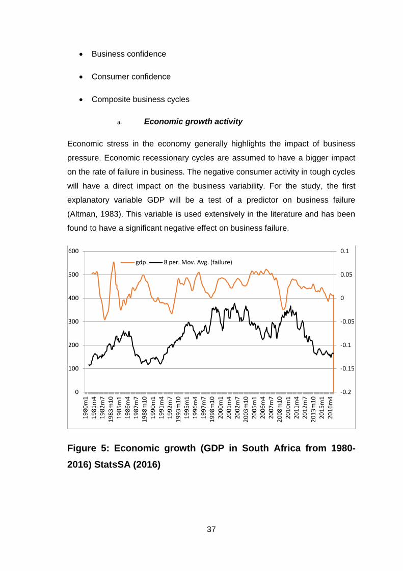
37
Business confidence
Consumer confidence
Composite business cycles
a. Economic growth activity
Economic stress in the economy generally highlights the impact of business
pressure. Economic recessionary cycles are assumed to have a bigger impact
on the rate of failure in business. The negative consumer activity in tough cycles
will have a direct impact on the business variability. For the study, the first
explanatory variable GDP will be a test of a predictor on business failure
(Altman, 1983). This variable is used extensively in the literature and has been
found to have a significant negative effect on business failure.
Figure 5: Economic growth (GDP in South Africa from 1980-
2016) StatsSA (2016)
-0.2
-0.15
-0.1
-0.05
0
0.05
0.1
0
100
200
300
400
500
600
19
80
m1
19
81
m4
19
82
m7
19
83
m1
0
19
85
m1
19
86
m4
19
87
m7
19
88
m1
0
19
90
m1
19
91
m4
19
92
m7
19
93
m1
0
19
95
m1
19
96
m4
19
97
m7
19
98
m1
0
20
00
m1
20
01
m4
20
02
m7
20
03
m1
0
20
05
m1
20
06
m4
20
07
m7
20
08
m1
02
01
0m
1
20
11
m4
20
12
m7
20
13
m1
0
20
15
m1
20
16
m4
gdp 8 per. Mov. Avg. (failure)
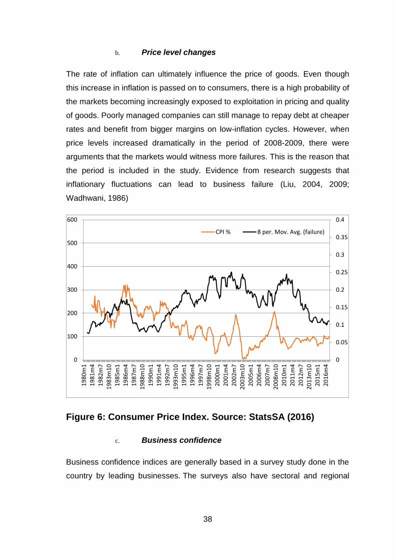
38
b. Price level changes
The rate of inflation can ultimately influence the price of goods. Even though
this increase in inflation is passed on to consumers, there is a high probability of
the markets becoming increasingly exposed to exploitation in pricing and quality
of goods. Poorly managed companies can still manage to repay debt at cheaper
rates and benefit from bigger margins on low-inflation cycles. However, when
price levels increased dramatically in the period of 2008-2009, there were
arguments that the markets would witness more failures. This is the reason that
the period is included in the study. Evidence from research suggests that
inflationary fluctuations can lead to business failure (Liu, 2004, 2009;
Wadhwani, 1986)
Figure 6: Consumer Price Index. Source: StatsSA (2016)
c. Business confidence
Business confidence indices are generally based in a survey study done in the
country by leading businesses. The surveys also have sectoral and regional
0
0.05
0.1
0.15
0.2
0.25
0.3
0.35
0.4
0
100
200
300
400
500
600
19
80
m1
19
81
m4
19
82
m7
19
83
m1
0
19
85
m1
19
86
m4
19
87
m7
19
88
m1
0
19
90
m1
19
91
m4
19
92
m7
19
93
m1
0
19
95
m1
19
96
m4
19
97
m7
19
98
m1
0
20
00
m1
20
01
m4
20
02
m7
20
03
m1
0
20
05
m1
20
06
m4
20
07
m7
20
08
m1
0
20
10
m1
20
11
m4
20
12
m7
20
13
m1
0
20
15
m1
20
16
m4
CPI % 8 per. Mov. Avg. (failure)
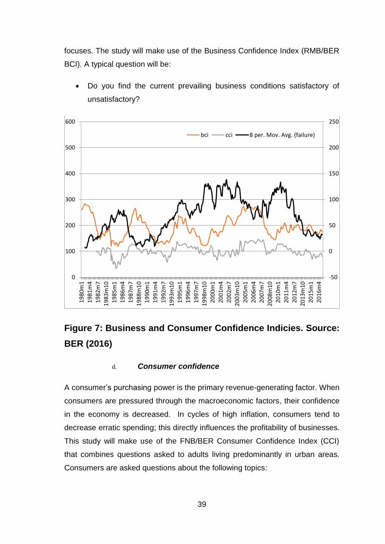
39
focuses. The study will make use of the Business Confidence Index (RMB/BER
BCI). A typical question will be:
Do you find the current prevailing business conditions satisfactory of
unsatisfactory?
Figure 7: Business and Consumer Confidence Indicies. Source:
BER (2016)
d. Consumer confidence
A consumer’s purchasing power is the primary revenue-generating factor. When
consumers are pressured through the macroeconomic factors, their confidence
in the economy is decreased. In cycles of high inflation, consumers tend to
decrease erratic spending; this directly influences the profitability of businesses.
This study will make use of the FNB/BER Consumer Confidence Index (CCI)
that combines questions asked to adults living predominantly in urban areas.
Consumers are asked questions about the following topics:
-50
0
50
100
150
200
250
0
100
200
300
400
500
600
19
80
m1
19
81
m4
19
82
m7
19
83
m1
0
19
85
m1
19
86
m4
19
87
m7
19
88
m1
0
19
90
m1
19
91
m4
19
92
m7
19
93
m1
0
19
95
m1
19
96
m4
19
97
m7
19
98
m1
0
20
00
m1
20
01
m4
20
02
m7
20
03
m1
0
20
05
m1
20
06
m4
20
07
m7
20
08
m1
0
20
10
m1
20
11
m4
20
12
m7
20
13
m1
0
20
15
m1
20
16
m4
bci cci 8 per. Mov. Avg. (failure)
40
Expectation of the performance in the economy
The financial position of the consumer
If the present time is it appropriate to buy durable goods
3.3 The population and data
This study is not restricted to specific types of industries. Secondary databases
as per Figure 1 will be used to extract and mine data via specified statistical
analysis software for the period of 1980-2016.
3.3.1 Quarterly data
Because our dependent variable of business failure is published on a monthly
cycle, quarterly data will be interpolated to monthly using the cubic spline
method. This will give the study finer details. According to Kershoff (2000), the
quarterly business confidence index cycle relationship with economic cycles has
proven to be a useful indicator for economic growth and has served as a strong
and leading indicator of business cycles in South Africa.
3.3.2 Business Failure
For this analysis, secondary data extracted from Stats SA will be used. Data will
only focus on the total number of liquidated companies and closed corporations.
Information published from Stats SA is sourced from the Registrar of
Companies and Close Corporations and Trade and Industry. These data sets
include both voluntary and compulsory liquidations of these businesses.
Liquidation refers to the winding-up of the affairs of a company or close
corporation when liabilities exceed assets and it can be resolved by voluntary
action or by an order of the court. A voluntary liquidation takes place when a
company or close corporation, by own choice, resolves to wind-up its affairs.
The business failure rates in numbers mimic closely the failures in percentage
(Chava & Jarrow, 2004). Given the purpose of this study to identify the
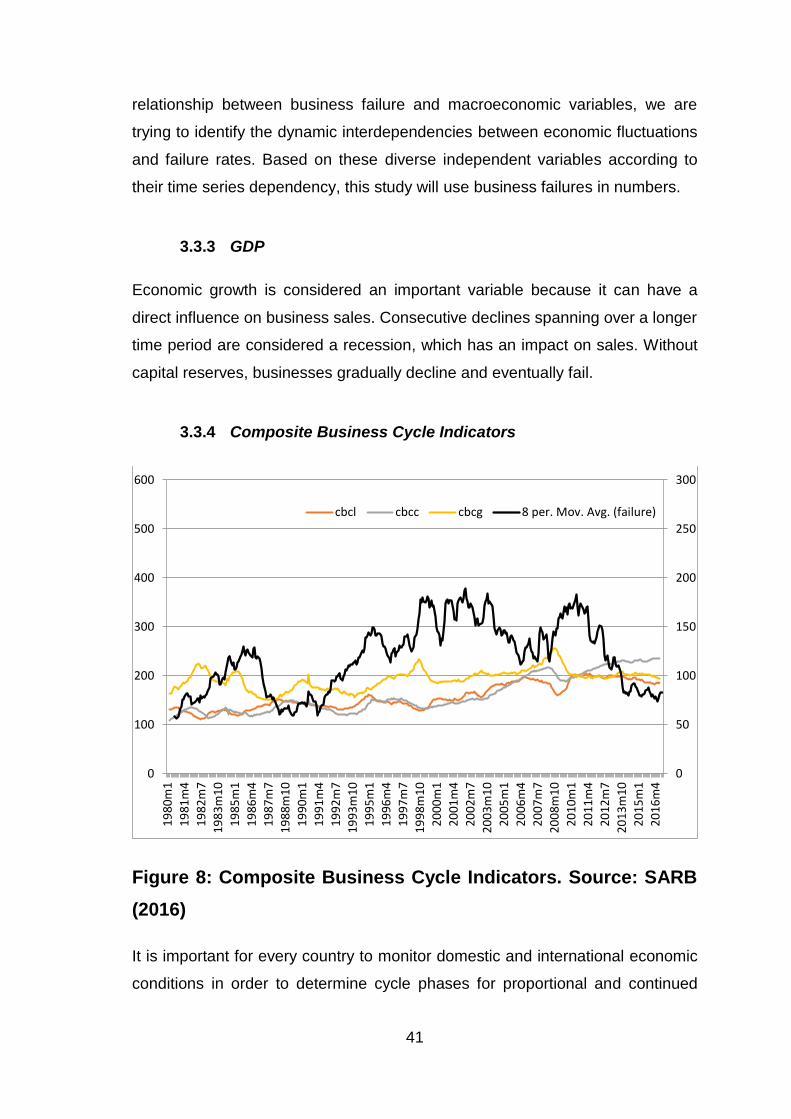
41
relationship between business failure and macroeconomic variables, we are
trying to identify the dynamic interdependencies between economic fluctuations
and failure rates. Based on these diverse independent variables according to
their time series dependency, this study will use business failures in numbers.
3.3.3 GDP
Economic growth is considered an important variable because it can have a
direct influence on business sales. Consecutive declines spanning over a longer
time period are considered a recession, which has an impact on sales. Without
capital reserves, businesses gradually decline and eventually fail.
3.3.4 Composite Business Cycle Indicators
Figure 8: Composite Business Cycle Indicators. Source: SARB
(2016)
It is important for every country to monitor domestic and international economic
conditions in order to determine cycle phases for proportional and continued
0
50
100
150
200
250
300
0
100
200
300
400
500
600
19
80
m1
19
81
m4
19
82
m7
19
83
m1
0
19
85
m1
19
86
m4
19
87
m7
19
88
m1
0
19
90
m1
19
91
m4
19
92
m7
19
93
m1
0
19
95
m1
19
96
m4
19
97
m7
19
98
m1
0
20
00
m1
20
01
m4
20
02
m7
20
03
m1
0
20
05
m1
20
06
m4
20
07
m7
20
08
m1
0
20
10
m1
20
11
m4
20
12
m7
20
13
m1
0
20
15
m1
20
16
m4
cbcl cbcc cbcg 8 per. Mov. Avg. (failure)
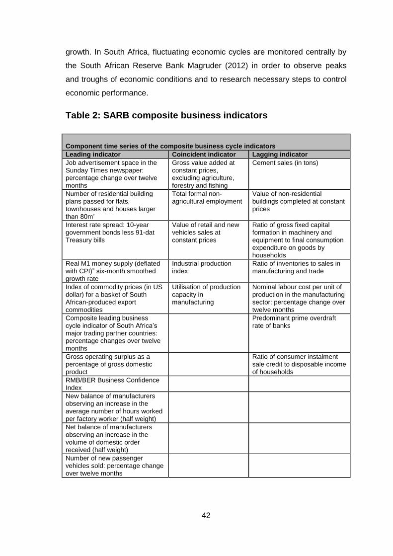
42
growth. In South Africa, fluctuating economic cycles are monitored centrally by
the South African Reserve Bank Magruder (2012) in order to observe peaks
and troughs of economic conditions and to research necessary steps to control
economic performance.
Table 2: SARB composite business indicators
Component time series of the composite business cycle indicators
Leading indicator Coincident indicator Lagging indicator
Job advertisement space in the Sunday Times newspaper: percentage change over twelve months
Gross value added at constant prices, excluding agriculture, forestry and fishing
Cement sales (in tons)
Number of residential building plans passed for flats, townhouses and houses larger than 80m’
Total formal non-agricultural employment
Value of non-residential buildings completed at constant prices
Interest rate spread: 10-year government bonds less 91-dat Treasury bills
Value of retail and new vehicles sales at constant prices
Ratio of gross fixed capital formation in machinery and equipment to final consumption expenditure on goods by households
Real M1 money supply (deflated with CPI)” six-month smoothed growth rate
Industrial production index
Ratio of inventories to sales in manufacturing and trade
Index of commodity prices (in US dollar) for a basket of South African-produced export commodities
Utilisation of production capacity in manufacturing
Nominal labour cost per unit of production in the manufacturing sector: percentage change over twelve months
Composite leading business cycle indicator of South Africa’s major trading partner countries: percentage changes over twelve months
Predominant prime overdraft rate of banks
Gross operating surplus as a percentage of gross domestic product
Ratio of consumer instalment sale credit to disposable income of households
RMB/BER Business Confidence Index
New balance of manufacturers observing an increase in the average number of hours worked per factory worker (half weight)
Net balance of manufacturers observing an increase in the volume of domestic order received (half weight)
Number of new passenger vehicles sold: percentage change over twelve months
43
3.3.5 Consumer Price Index (CPI)
Inflation can be contradictory in its effects on aggregate business failure rates.
The contentious issue with inflation is that it can be two-fold. Altman (1983)
argued that inflation can be inversely correlated with business failure rates
because businesses can repay their debt quicker by paying less interest.
However, lower inflation can cause less competition within the micro and macro
environments. So, inflation can cause more failure rates by influencing the
business’s earnings, ultimately diminishing the capability to repay its debt
(Wadhwani, 1986). In this way, inflation can lead to higher business
bankruptcies too (Liu, 2004, 2009; Wadhwani, 1986). This is the reason inflation
is included in the current study.
3.3.6 Business Confidence (BCI - RMB/BER BCI: Business
confidence index)
BER takes the percentage of respondents that rate prevailing conditions as
satisfactory as the indicator or proxy of business confidence. The
composite RMB/BER Business Confidence Index (BCI) is the unweighted mean
of five sectoral indices, namely manufacturing, building, contracting, retail,
wholesale and new vehicle dealers. Business confidence can vary between 0
and 100, where 0 indicates an extreme lack of confidence, 50 indicates
neutrality, and 100 indicate extreme confidence.
3.3.7 Consumer Confidence (FNB/BER CCI: Consumer confidence
index)
CCI has provided detailed data on consumer confidence that is disaggregated
by income, Living Standards Measure, and population groups
Consumer confidence is expressed as a net balance, which is calculated as the
percentage of respondents expecting an improvement (good time to buy
durable goods), less the percentage expecting a deterioration (bad time to buy
durable goods). CCI is measure on a scale of between 0 – 100.
44
3.4 Methods
This study adopts a quantitative approach, which will facilitate the use of
secondary data through statistical analyses.
3.5 Model strategy
Liu (2004) and Vlieghe (2001) addressed the shortcomings of separating the
short-run and long-run reactions of business failure relating to macroeconomic
variables by introducing time-series cointegration and error correction models.
Supporting this, Santoro and Gaffeo (2009) argue that this research has an
empirical importance and can contribute to the implications of theoretical
models of economic and productivity growth. They have also indicated that
from an economic point of view, the analysis follows three distinct steps. First,
variables must be tested for stochastic properties by means of panel unit root
tests. This study will use the Augmented Dickey Fuller test for stationarity
(ADF). Secondly, the model will test for cointegration among the identified
variables and for this the analyses the study will use the Johansen test for Co-
Integration. This test will assess if there is a long-run relationship. Third, the
residuals of the integration step were used to test as an n error correction term
with a panel (VECM).
Additionally the study will propose if business failure can be predicted through
the business cycles mirroring Santoro and Gaffeo (2009) study for long-run
growth. For this test Granger Causality will be formulated. Finally, the study will
incorporate a lag within the variables. Zavgren (1985) was sceptical about
solely focusing on the financial ratios to predict business failure and introduced
the presence of a time lag in receiving these financial factors.
3.5.1 Augmented Dickey Fuller (ADF) test for stationarity
The Augmented Dickey Fuller Test was conducted to assess the stationarity of
time series variables. This is vital to ensure that the series are stationary before
45
any model is fitted; otherwise the relationship that will be determined using the
model will be inaccurate.
Non-stationarity and data instability may have severe effects for the traditional
failure prediction models that can lead to poor predictive abilities in future dated
samples (Mensah, 1984). Additionally, data instability causes prediction models
to be unstable and fragile over time will cause other coefficients on new data.
Consequently, traditional prediction models may need redevelopment and
updating (Joy & Tollefson, 1975; Keasey & Watson, 1991; Mensah, 1984;
Taffler, 1982). Lastly, traditional failure prediction models based on pooled
estimation samples may be constructed on distorted data, resulting in
inconsistent coefficient estimates that can lead to low accuracy levels. (Platt,
Platt, & Pedersen, 1994)
Co-integration implies that the linear combination of some nonstationary time
series is stationary. The plots of the time-series movements of the independent
variables and failure rates can potentially drift together and suggest that they
may be co-integrated. To establish co-integration, we first test whether each
series contains a unit root and is integrated in each sub-period using the
augmented Dickey–Fuller (ADF) test.
3.5.2 The Johansen test for co-integration
The Johansen test for Co-Integration was conducted to assess if there was a
long-term equilibrium relationship between failure and each of the independent
variables. This is to test if the variables move together, that is, if one variable
increases the other one increase, or the former decreases back to the same
level with the latter.
3.5.3 The Vector Error Correction Model (VCEM)
The Vector Error Correction Model was fitted to assess whether there was a
long-term relationship between failure and each of the other variables. The
presence of cointegration between variables would have suggested there being
46
a long-term relationship between the variables. The VECM assesses the
relationship but does not assess the direction of the relationship.
3.5.4 Granger Causality
Granger causality is a model in which the past values of variable A contains
information that can be used to predict the future values of another variable B.
In that case, past values of B will contain less information to predict future
values of B than the combination of past values for A and B. If that is the case,
A is said to granger cause B. In other words, granger causality assesses the
direction of the relationship
Unlike linear regression where the r-square is very important, in time series the
standard regression fails when dealing with non-stationary variables. The
regression of time series produces spurious regressions that suggest
relationships even when there are none. Thus r-square is not very useful.
The conceptualisation of the Granger Causality is attributed to the works of
Wiener (1956) who conceived the notion as a scientific approach to
demonstrating knowledge and understanding in scientific research. Ganger
causality is premised on the fact that if predictions in a particular time series are
enhanced in a scientific study by incorporating the knowledge of an additional
series to the existing one, the later series is said to influence the outcomes of
the previous one. This idea was later formalised by Granger (1980) using linear
regression models to approve the correlational approaches attributed to
formulation. The improvement of the predictions is then undertaken by
determining the ratio of the variance in the error terms. If the ratio is larger than
one, then there is an improvement in the second time series, thus qualifying a
causal connection between series one and two.
Granger causality is significantly important to this study since it investigates the
cause-effect relationships between the macroeconomic factors in South Africa
and failures in businesses. To understand the relationship between the changes
in macroeconomic factors and business failures, we are investigating the causal
effects of macroeconomic fluctuations on business failure in South Africa, a
47
factor which qualifies the use of Granger Causality for this research. The
Granger Causality is utilised to establish whether or not the macroeconomic
variables investigated in this study can be employed to predict the probability of
business failures. This is based on the assumption that macroeconomic factors
contribute to business failure. In undertaking these effects, f-tests will be used
to determine the lag effects of the business failure approach following
fluctuations in explanatory variables.
3.6 Limitations of datasets
- The study will focus only on private companies and close corporations
- The interpolation of quarterly data can potentially lean to bias
- Business failure does not happen overnight and in general, panel data
can specify the date at which the company was officially liquidated and
did not consider the process of company failure.
3.7 The validity and reliability of research
The reliability and validity scales of research qualities are important aspects of
research studies, which determine the extent to which the results obtained are
meaningful to the end consumer. A research study is considered reliable when
it gives similar results when tested on the population with the same
characteristics at different times. This section discusses the validity and
reliability conditions ensured in this study.
3.7.1 Validity
Validity of a research study defines the accuracy of a measure used as a
variable or just the extent to which the scores obtained from an analysis
represent the real concept studied. That is, the extent to which the models used
is capable of testing the factors as designed. There are three types of research
48
validities with which researchers must be concerned. These are discussed in
the subsequent sections of this study.
a. Face validity
Face validity or content validity defines the level of agreement between the
experts in a particular field that a certain truth is proven within the realms of the
available knowledge. In this definition, the face validity concept ensures the
usefulness and accuracy of a given method in achieving the desired outcome
based on the consideration of previous research.
To ensure face validity in this study, a comprehensive review of the previous
literature has been performed to establish the similarities between the ideas and
methodologies used in the current research as recommended and utilised by
various researchers in other studies. Additionally, an extensive consultation with
experts has also been conducted prior to and after performing the literature
review to validate the findings obtained, presented, and utilised in deriving the
success of this study. Triangulation method, used and recommended by
Thomas and Magilvy (2011), has been utilised in coming up with the
appropriate verifications of the current study.
b. Internal validity
The internal validity of research illustrates the researcher’s attempt to ensure
that the data collected and analysed are free from biases and thus reflect the
true opinions and facts of the study (Thomas & Magilvy, 2011). Although it is
assumed that the information collected will be factual, the data and information
acquired from various databases will not be edited in order to maintain their
authenticity and reliability for use.
c. External validity
The external validity describes the extent to which the findings of a research
study can be replicated and thus be generalised as true representations of the
scenario in the studied population (Thomas & Magilvy, 2011). A wide array of
historical data on industries across the various regions spanning from 1980 to
49
2016 will enhance accuracy and thus guarantee representativeness and
reliability for replicability purposes. The large sample size (all private
corporations) and the longitudinal approach to data collection will ensure
external validity.
3.7.2 Reliability
The reliability aspect of research, on the other hand, defines how consistent the
findings of a scientific research study are for the accuracy of the methods of
data collection and data analysis adopted (Bush, 2007). In this way, the
reliability of a research study is a measure of the internal consistency of the
research findings. According to Hair et al. (2006) , the reliability is a test of the
degree of consistency exhibited in different measurements of the response from
an individual versus the idea of ensuring that the responses provided maintain
the consistency and similarity across different situations and times. That is, if
the same test was performed under the same scenario with the same
circumstances, similar results should be obtained. This is what Bush (2007)
referred to as the test-retest method. Although there are several methods used
to test for reliability, this study uses the most common one: the Cronbach alpha
coefficient with 0.7 used as the minimal acceptance level for reliability.
Specifically, the reliability of the data and the information obtained in this study
will be guaranteed by using static, public data drawn from authentic sources
and used in their original forms without editing. They can then be verified easily
through statistical analyses.
3.7.3 Ethical considerations
Before beginning to collect data and subsequent analysis, the researcher will
seek permission and approval for research from the Ethics Committee to ensure
compliance with ethical regulations of research throughout the session. Once
used, the collected information will be destroyed through burning to maintain
required privacy.
50
4 CHAPTER 4: PRESENTATION OF RESULTS
This chapter will include details of the data used, analysis of data, and
interpretation. For this purpose, tools used for analysis, method of analysis, and
the results of analysis are explained. Investigating the effects of how
macroeconomic factors influence business failure (failure), the study
incorporates macroeconomic variables in a 3-phased approach. In the first
phase, the study will include general macro variables including Gross Domestic
Product (GDP) and Consumer Price Index (CPI). In the second phase, the
analysis will be done using composite business cycle variables published by the
South African Reserve Bank. These variables include the composite leading
(CBCL), composite coincident- (CBCC), and composite lagging (CBCG)
business cycle indicator. In the third phase, the study will adopt a more
behavioural indicator based on surveys done in the relevant sectors, namely
Business Confidence Index (BCI) and Consumer Confidence Index (CCI)
developed by the Bureau for Economic Research (BER). Longitudinal data for
this study was used over a period of 36 years ranging from 1980 to 2016.
In this empirical study, data analysis was done using the Vector Error
Correction Model (VECM) to look at the relationship between business failures
and the considered macroeconomic factors, and the interactions between these
respective dependent and independent variables. Liu (2009) adopted a Vector
Auto Regression (VAR) approach and argued that using VAR models is a
suitable approach to analyse the dynamics of business failures in the business
cycles. Liu (2009) also observed the interactions between the systems of
macroeconomic variables and business failure. According to the researcher, it is
well-known that the majority of economic panel data is non-stationary, although
in the long run it tends to be cointegrated.
If a VAR has a cointegration specification, it restricts the long run convergence
of endogenous variables to their relationship, while allowing for a wide range of
short-run dynamics. As mentioned above, Liu (2009) supports Santoro and
Gaffeo (2009) by introducing the Engle and Granger (1987) representation
theorem where one first needs to establish if the series contain a unit root and is
51
integrated in each sub-period, using the ADF test. Liu (2009) used the
Johansen (1988) model to test the number of cointegrating vectors. This test
was done on the maximum eigenvalues and tested the null hypothesis.
The experimental methodology adopted in this study was the same strategy as
what Liu (2009) analysed in his study of macroeconomic risk. The study uses
the VAR model as a convenient way to analyse the relationship and interactions
between business failure and macroeconomic variables. Because it is well-
known that a majority of economic series data is non-stationary, to include a
case of potential long-run cointegration this study will be adopting the VECM.
The benefits of the VECM are that the resulting VAR from VECM representation
has more efficient coefficient estimates.
4.1 Data preparation
The subsequent sections detail the steps followed in preparing the data and
analysing it.
4.1.1 Interpolating data
Cubic Spline Interpolation was used to obtain estimates of data between known
data points. Thus, cubic splining of quarterly figures were used to generate
monthly estimates. According to Chava and Jarrow (2004) the use of monthly
observation intervals will distinctly improve the predictability of the models used.
This study’s dependent variable of business failure is published monthly, and
that is why the quarterly data to monthly has been interpolated, to improve the
number of observations. Only GDP, BCI and CCI were interpolated using the
cubic spline interpolation method.
4.1.2 Time series plots
A time series plot CBCL, CBCG, CCI, CPI, CBCC and BCI, together with the
number of business failures (Failure) shown below, discloses that the series are
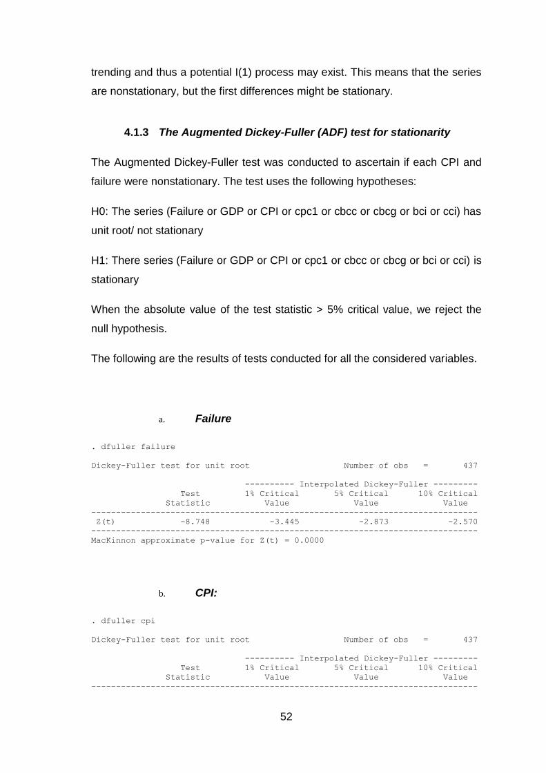
52
trending and thus a potential I(1) process may exist. This means that the series
are nonstationary, but the first differences might be stationary.
4.1.3 The Augmented Dickey-Fuller (ADF) test for stationarity
The Augmented Dickey-Fuller test was conducted to ascertain if each CPI and
failure were nonstationary. The test uses the following hypotheses:
H0: The series (Failure or GDP or CPI or cpc1 or cbcc or cbcg or bci or cci) has
unit root/ not stationary
H1: There series (Failure or GDP or CPI or cpc1 or cbcc or cbcg or bci or cci) is
stationary
When the absolute value of the test statistic > 5% critical value, we reject the
null hypothesis.
The following are the results of tests conducted for all the considered variables.
a. Failure
. dfuller failure
Dickey-Fuller test for unit root Number of obs = 437
---------- Interpolated Dickey-Fuller ---------
Test 1% Critical 5% Critical 10% Critical
Statistic Value Value Value
------------------------------------------------------------------------------
Z(t) -8.748 -3.445 -2.873 -2.570
------------------------------------------------------------------------------
MacKinnon approximate p-value for Z(t) = 0.0000
b. CPI:
. dfuller cpi
Dickey-Fuller test for unit root Number of obs = 437
---------- Interpolated Dickey-Fuller ---------
Test 1% Critical 5% Critical 10% Critical
Statistic Value Value Value
------------------------------------------------------------------------------
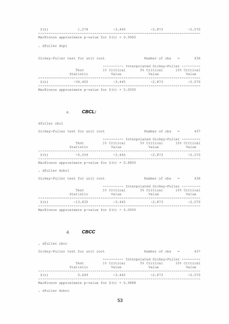
53
Z(t) 1.278 -3.445 -2.873 -2.570
------------------------------------------------------------------------------
MacKinnon approximate p-value for Z(t) = 0.9965
. dfuller dcpi
Dickey-Fuller test for unit root Number of obs = 436
---------- Interpolated Dickey-Fuller ---------
Test 1% Critical 5% Critical 10% Critical
Statistic Value Value Value
------------------------------------------------------------------------------
Z(t) -34.455 -3.445 -2.873 -2.570
------------------------------------------------------------------------------
MacKinnon approximate p-value for Z(t) = 0.0000
c. CBCL:
dfuller cbcl
Dickey-Fuller test for unit root Number of obs = 437
---------- Interpolated Dickey-Fuller ---------
Test 1% Critical 5% Critical 10% Critical
Statistic Value Value Value
------------------------------------------------------------------------------
Z(t) -0.559 -3.445 -2.873 -2.570
------------------------------------------------------------------------------
MacKinnon approximate p-value for Z(t) = 0.8800
. dfuller dcbcl
Dickey-Fuller test for unit root Number of obs = 436
---------- Interpolated Dickey-Fuller ---------
Test 1% Critical 5% Critical 10% Critical
Statistic Value Value Value
------------------------------------------------------------------------------
Z(t) -13.835 -3.445 -2.873 -2.570
------------------------------------------------------------------------------
MacKinnon approximate p-value for Z(t) = 0.0000
d. CBCC
. dfuller cbcc
Dickey-Fuller test for unit root Number of obs = 437
---------- Interpolated Dickey-Fuller ---------
Test 1% Critical 5% Critical 10% Critical
Statistic Value Value Value
------------------------------------------------------------------------------
Z(t) 0.649 -3.445 -2.873 -2.570
------------------------------------------------------------------------------
MacKinnon approximate p-value for Z(t) = 0.9888
. dfuller dcbcc
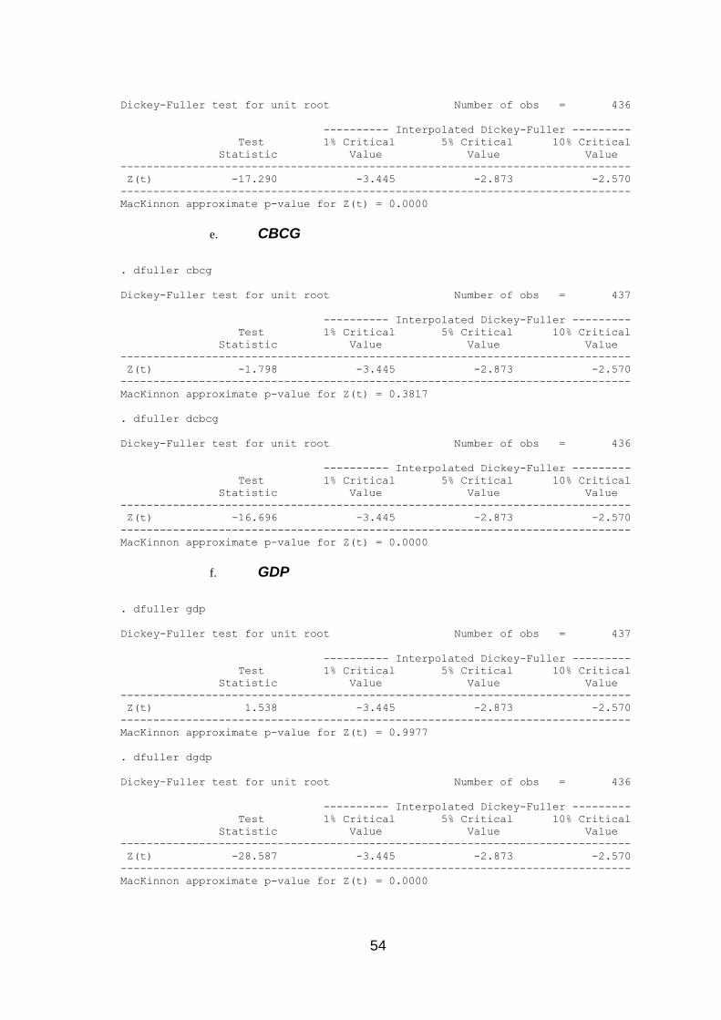
54
Dickey-Fuller test for unit root Number of obs = 436
---------- Interpolated Dickey-Fuller ---------
Test 1% Critical 5% Critical 10% Critical
Statistic Value Value Value
------------------------------------------------------------------------------
Z(t) -17.290 -3.445 -2.873 -2.570
------------------------------------------------------------------------------
MacKinnon approximate p-value for Z(t) = 0.0000
e. CBCG
. dfuller cbcg
Dickey-Fuller test for unit root Number of obs = 437
---------- Interpolated Dickey-Fuller ---------
Test 1% Critical 5% Critical 10% Critical
Statistic Value Value Value
------------------------------------------------------------------------------
Z(t) -1.798 -3.445 -2.873 -2.570
------------------------------------------------------------------------------
MacKinnon approximate p-value for Z(t) = 0.3817
. dfuller dcbcg
Dickey-Fuller test for unit root Number of obs = 436
---------- Interpolated Dickey-Fuller ---------
Test 1% Critical 5% Critical 10% Critical
Statistic Value Value Value
------------------------------------------------------------------------------
Z(t) -16.696 -3.445 -2.873 -2.570
------------------------------------------------------------------------------
MacKinnon approximate p-value for Z(t) = 0.0000
f. GDP
. dfuller gdp
Dickey-Fuller test for unit root Number of obs = 437
---------- Interpolated Dickey-Fuller ---------
Test 1% Critical 5% Critical 10% Critical
Statistic Value Value Value
------------------------------------------------------------------------------
Z(t) 1.538 -3.445 -2.873 -2.570
------------------------------------------------------------------------------
MacKinnon approximate p-value for Z(t) = 0.9977
. dfuller dgdp
Dickey-Fuller test for unit root Number of obs = 436
---------- Interpolated Dickey-Fuller ---------
Test 1% Critical 5% Critical 10% Critical
Statistic Value Value Value
------------------------------------------------------------------------------
Z(t) -28.587 -3.445 -2.873 -2.570
------------------------------------------------------------------------------
MacKinnon approximate p-value for Z(t) = 0.0000
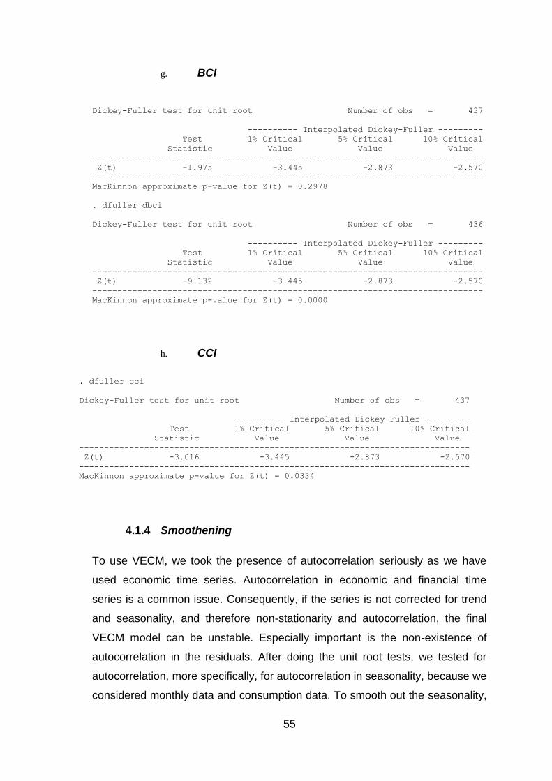
55
g. BCI
Dickey-Fuller test for unit root Number of obs = 437
---------- Interpolated Dickey-Fuller ---------
Test 1% Critical 5% Critical 10% Critical
Statistic Value Value Value
------------------------------------------------------------------------------
Z(t) -1.975 -3.445 -2.873 -2.570
------------------------------------------------------------------------------
MacKinnon approximate p-value for Z(t) = 0.2978
. dfuller dbci
Dickey-Fuller test for unit root Number of obs = 436
---------- Interpolated Dickey-Fuller ---------
Test 1% Critical 5% Critical 10% Critical
Statistic Value Value Value
------------------------------------------------------------------------------
Z(t) -9.132 -3.445 -2.873 -2.570
------------------------------------------------------------------------------
MacKinnon approximate p-value for Z(t) = 0.0000
h. CCI
. dfuller cci
Dickey-Fuller test for unit root Number of obs = 437
---------- Interpolated Dickey-Fuller ---------
Test 1% Critical 5% Critical 10% Critical
Statistic Value Value Value
------------------------------------------------------------------------------
Z(t) -3.016 -3.445 -2.873 -2.570
------------------------------------------------------------------------------
MacKinnon approximate p-value for Z(t) = 0.0334
4.1.4 Smoothening
To use VECM, we took the presence of autocorrelation seriously as we have
used economic time series. Autocorrelation in economic and financial time
series is a common issue. Consequently, if the series is not corrected for trend
and seasonality, and therefore non-stationarity and autocorrelation, the final
VECM model can be unstable. Especially important is the non-existence of
autocorrelation in the residuals. After doing the unit root tests, we tested for
autocorrelation, more specifically, for autocorrelation in seasonality, because we
considered monthly data and consumption data. To smooth out the seasonality,
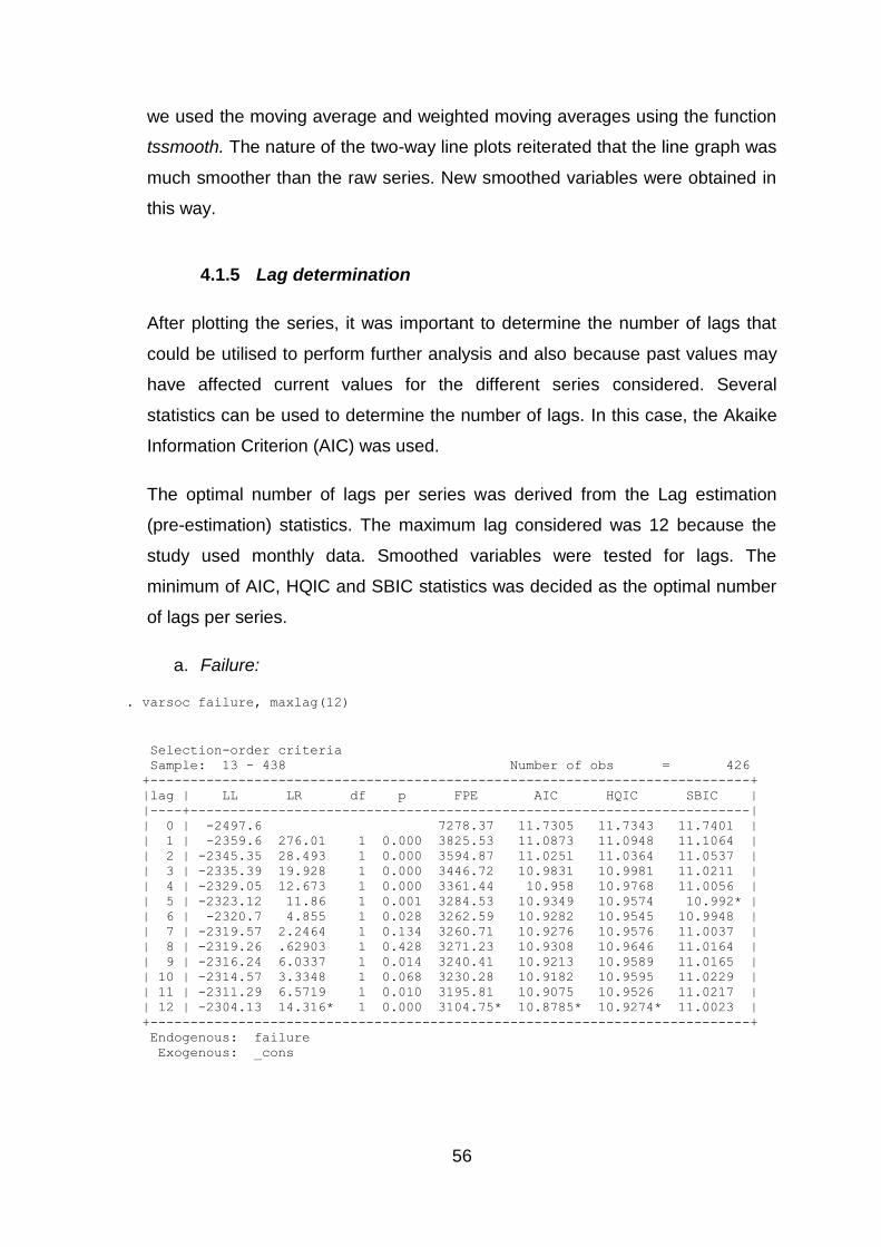
56
we used the moving average and weighted moving averages using the function
tssmooth. The nature of the two-way line plots reiterated that the line graph was
much smoother than the raw series. New smoothed variables were obtained in
this way.
4.1.5 Lag determination
After plotting the series, it was important to determine the number of lags that
could be utilised to perform further analysis and also because past values may
have affected current values for the different series considered. Several
statistics can be used to determine the number of lags. In this case, the Akaike
Information Criterion (AIC) was used.
The optimal number of lags per series was derived from the Lag estimation
(pre-estimation) statistics. The maximum lag considered was 12 because the
study used monthly data. Smoothed variables were tested for lags. The
minimum of AIC, HQIC and SBIC statistics was decided as the optimal number
of lags per series.
a. Failure:
. varsoc failure, maxlag(12)
Selection-order criteria
Sample: 13 - 438 Number of obs = 426
+---------------------------------------------------------------------------+
|lag | LL LR df p FPE AIC HQIC SBIC |
|----+----------------------------------------------------------------------|
| 0 | -2497.6 7278.37 11.7305 11.7343 11.7401 |
| 1 | -2359.6 276.01 1 0.000 3825.53 11.0873 11.0948 11.1064 |
| 2 | -2345.35 28.493 1 0.000 3594.87 11.0251 11.0364 11.0537 |
| 3 | -2335.39 19.928 1 0.000 3446.72 10.9831 10.9981 11.0211 |
| 4 | -2329.05 12.673 1 0.000 3361.44 10.958 10.9768 11.0056 |
| 5 | -2323.12 11.86 1 0.001 3284.53 10.9349 10.9574 10.992* |
| 6 | -2320.7 4.855 1 0.028 3262.59 10.9282 10.9545 10.9948 |
| 7 | -2319.57 2.2464 1 0.134 3260.71 10.9276 10.9576 11.0037 |
| 8 | -2319.26 .62903 1 0.428 3271.23 10.9308 10.9646 11.0164 |
| 9 | -2316.24 6.0337 1 0.014 3240.41 10.9213 10.9589 11.0165 |
| 10 | -2314.57 3.3348 1 0.068 3230.28 10.9182 10.9595 11.0229 |
| 11 | -2311.29 6.5719 1 0.010 3195.81 10.9075 10.9526 11.0217 |
| 12 | -2304.13 14.316* 1 0.000 3104.75* 10.8785* 10.9274* 11.0023 |
+---------------------------------------------------------------------------+
Endogenous: failure
Exogenous: _cons
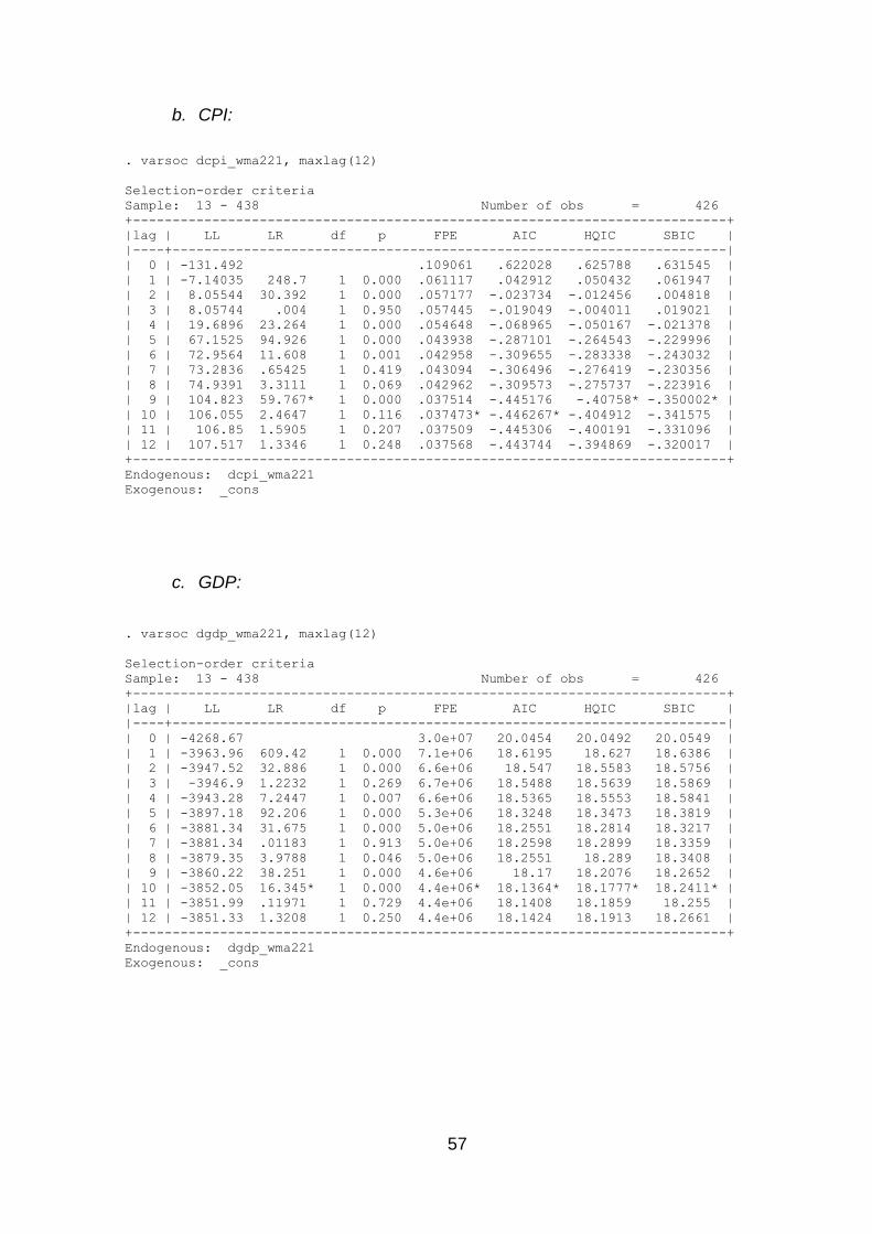
57
b. CPI:
. varsoc dcpi_wma221, maxlag(12)
Selection-order criteria
Sample: 13 - 438 Number of obs = 426
+---------------------------------------------------------------------------+
|lag | LL LR df p FPE AIC HQIC SBIC |
|----+----------------------------------------------------------------------|
| 0 | -131.492 .109061 .622028 .625788 .631545 |
| 1 | -7.14035 248.7 1 0.000 .061117 .042912 .050432 .061947 |
| 2 | 8.05544 30.392 1 0.000 .057177 -.023734 -.012456 .004818 |
| 3 | 8.05744 .004 1 0.950 .057445 -.019049 -.004011 .019021 |
| 4 | 19.6896 23.264 1 0.000 .054648 -.068965 -.050167 -.021378 |
| 5 | 67.1525 94.926 1 0.000 .043938 -.287101 -.264543 -.229996 |
| 6 | 72.9564 11.608 1 0.001 .042958 -.309655 -.283338 -.243032 |
| 7 | 73.2836 .65425 1 0.419 .043094 -.306496 -.276419 -.230356 |
| 8 | 74.9391 3.3111 1 0.069 .042962 -.309573 -.275737 -.223916 |
| 9 | 104.823 59.767* 1 0.000 .037514 -.445176 -.40758* -.350002* |
| 10 | 106.055 2.4647 1 0.116 .037473* -.446267* -.404912 -.341575 |
| 11 | 106.85 1.5905 1 0.207 .037509 -.445306 -.400191 -.331096 |
| 12 | 107.517 1.3346 1 0.248 .037568 -.443744 -.394869 -.320017 |
+---------------------------------------------------------------------------+
Endogenous: dcpi_wma221
Exogenous: _cons
c. GDP:
. varsoc dgdp_wma221, maxlag(12)
Selection-order criteria
Sample: 13 - 438 Number of obs = 426
+---------------------------------------------------------------------------+
|lag | LL LR df p FPE AIC HQIC SBIC |
|----+----------------------------------------------------------------------|
| 0 | -4268.67 3.0e+07 20.0454 20.0492 20.0549 |
| 1 | -3963.96 609.42 1 0.000 7.1e+06 18.6195 18.627 18.6386 |
| 2 | -3947.52 32.886 1 0.000 6.6e+06 18.547 18.5583 18.5756 |
| 3 | -3946.9 1.2232 1 0.269 6.7e+06 18.5488 18.5639 18.5869 |
| 4 | -3943.28 7.2447 1 0.007 6.6e+06 18.5365 18.5553 18.5841 |
| 5 | -3897.18 92.206 1 0.000 5.3e+06 18.3248 18.3473 18.3819 |
| 6 | -3881.34 31.675 1 0.000 5.0e+06 18.2551 18.2814 18.3217 |
| 7 | -3881.34 .01183 1 0.913 5.0e+06 18.2598 18.2899 18.3359 |
| 8 | -3879.35 3.9788 1 0.046 5.0e+06 18.2551 18.289 18.3408 |
| 9 | -3860.22 38.251 1 0.000 4.6e+06 18.17 18.2076 18.2652 |
| 10 | -3852.05 16.345* 1 0.000 4.4e+06* 18.1364* 18.1777* 18.2411* |
| 11 | -3851.99 .11971 1 0.729 4.4e+06 18.1408 18.1859 18.255 |
| 12 | -3851.33 1.3208 1 0.250 4.4e+06 18.1424 18.1913 18.2661 |
+---------------------------------------------------------------------------+
Endogenous: dgdp_wma221
Exogenous: _cons
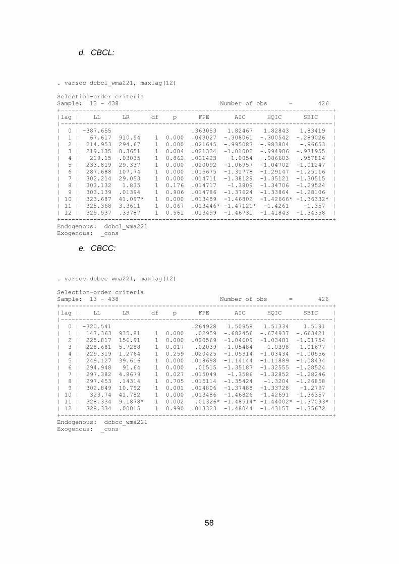
58
d. CBCL:
. varsoc dcbcl_wma221, maxlag(12)
Selection-order criteria
Sample: 13 - 438 Number of obs = 426
+---------------------------------------------------------------------------+
|lag | LL LR df p FPE AIC HQIC SBIC |
|----+----------------------------------------------------------------------|
| 0 | -387.655 .363053 1.82467 1.82843 1.83419 |
| 1 | 67.617 910.54 1 0.000 .043027 -.308061 -.300542 -.289026 |
| 2 | 214.953 294.67 1 0.000 .021645 -.995083 -.983804 -.96653 |
| 3 | 219.135 8.3651 1 0.004 .021324 -1.01002 -.994986 -.971955 |
| 4 | 219.15 .03035 1 0.862 .021423 -1.0054 -.986603 -.957814 |
| 5 | 233.819 29.337 1 0.000 .020092 -1.06957 -1.04702 -1.01247 |
| 6 | 287.688 107.74 1 0.000 .015675 -1.31778 -1.29147 -1.25116 |
| 7 | 302.214 29.053 1 0.000 .014711 -1.38129 -1.35121 -1.30515 |
| 8 | 303.132 1.835 1 0.176 .014717 -1.3809 -1.34706 -1.29524 |
| 9 | 303.139 .01394 1 0.906 .014786 -1.37624 -1.33864 -1.28106 |
| 10 | 323.687 41.097* 1 0.000 .013489 -1.46802 -1.42666* -1.36332* |
| 11 | 325.368 3.3611 1 0.067 .013446* -1.47121* -1.4261 -1.357 |
| 12 | 325.537 .33787 1 0.561 .013499 -1.46731 -1.41843 -1.34358 |
+---------------------------------------------------------------------------+
Endogenous: dcbcl_wma221
Exogenous: _cons
e. CBCC:
. varsoc dcbcc_wma221, maxlag(12)
Selection-order criteria
Sample: 13 - 438 Number of obs = 426
+---------------------------------------------------------------------------+
|lag | LL LR df p FPE AIC HQIC SBIC |
|----+----------------------------------------------------------------------|
| 0 | -320.541 .264928 1.50958 1.51334 1.5191 |
| 1 | 147.363 935.81 1 0.000 .02959 -.682456 -.674937 -.663421 |
| 2 | 225.817 156.91 1 0.000 .020569 -1.04609 -1.03481 -1.01754 |
| 3 | 228.681 5.7288 1 0.017 .02039 -1.05484 -1.0398 -1.01677 |
| 4 | 229.319 1.2764 1 0.259 .020425 -1.05314 -1.03434 -1.00556 |
| 5 | 249.127 39.616 1 0.000 .018698 -1.14144 -1.11889 -1.08434 |
| 6 | 294.948 91.64 1 0.000 .01515 -1.35187 -1.32555 -1.28524 |
| 7 | 297.382 4.8679 1 0.027 .015049 -1.3586 -1.32852 -1.28246 |
| 8 | 297.453 .14314 1 0.705 .015114 -1.35424 -1.3204 -1.26858 |
| 9 | 302.849 10.792 1 0.001 .014806 -1.37488 -1.33728 -1.2797 |
| 10 | 323.74 41.782 1 0.000 .013486 -1.46826 -1.42691 -1.36357 |
| 11 | 328.334 9.1878* 1 0.002 .01326* -1.48514* -1.44002* -1.37093* |
| 12 | 328.334 .00015 1 0.990 .013323 -1.48044 -1.43157 -1.35672 |
+---------------------------------------------------------------------------+
Endogenous: dcbcc_wma221
Exogenous: _cons
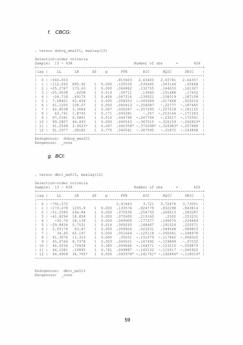
59
f. CBCG:
. varsoc dcbcg_wma221, maxlag(12)
Selection-order criteria
Sample: 13 - 438 Number of obs = 426
+---------------------------------------------------------------------------+
|lag | LL LR df p FPE AIC HQIC SBIC |
|----+----------------------------------------------------------------------|
| 0 | -560.053 .815603 2.63405 2.63781 2.64357 |
| 1 | -112.092 895.92 1 0.000 .100035 .535645 .543164 .55468 |
| 2 | -25.2767 173.63 1 0.000 .066862 .132755 .144033 .161307 |
| 3 | -25.0638 .4258 1 0.514 .06711 .13645 .151488 .17452 |
| 4 | -24.718 .69175 1 0.406 .067316 .139521 .158319 .187108 |
| 5 | 7.08401 63.604 1 0.000 .058253 -.005089 .017468 .052016 |
| 6 | 61.1205 108.07 1 0.000 .045413 -.254087 -.22777 -.187465 |
| 7 | 62.8038 3.3666 1 0.067 .045267 -.257295 -.227218 -.181155 |
| 8 | 63.741 1.8745 1 0.171 .045281 -.257 -.223164 -.171343 |
| 9 | 67.0341 6.5861 1 0.010 .044796 -.267766 -.23017 -.172591 |
| 10 | 89.2807 44.493 1 0.000 .040543 -.367515 -.326159 -.262823* |
| 11 | 91.2568 3.9523* 1 0.047 .040358* -.372098* -.326983* -.257888 |
| 12 | 91.2977 .08182 1 0.775 .040541 -.367595 -.31872 -.243868 |
+---------------------------------------------------------------------------+
Endogenous: dcbcg_wma221
Exogenous: _cons
g. BCI:
. varsoc dbci_ma515, maxlag(12)
Selection-order criteria
Sample: 13 - 438 Number of obs = 426
+---------------------------------------------------------------------------+
|lag | LL LR df p FPE AIC HQIC SBIC |
|----+----------------------------------------------------------------------|
| 0 | -791.572 2.41843 3.721 3.72476 3.73051 |
| 1 | -173.678 1235.8 1 0.000 .133574 .824779 .832298 .843814 |
| 2 | -51.2585 244.84 1 0.000 .075536 .254735 .266013 .283287 |
| 3 | -41.8294 18.858 1 0.000 .072605 .215162 .2302 .253231 |
| 4 | -32.76 18.139 1 0.000 .069906 .177277 .196075 .224864 |
| 5 | -29.8834 5.7531 1 0.016 .069293 .168467 .191024 .225571 |
| 6 | 2.05179 63.87 1 0.000 .059926 .023231 .049548 .089853 |
| 7 | 34.65 65.197 1 0.000 .051664 -.125118 -.095041 -.048978 |
| 8 | 41.3076 13.315 1 0.000 .05031 -.151679 -.117842 -.066022 |
| 9 | 45.6764 8.7378 1 0.003 .049521 -.167495 -.129899 -.07232 |
| 10 | 46.0536 .75428 1 0.385 .049666 -.164571 -.123215 -.059879 |
| 11 | 46.1081 .10895 1 0.741 .049887 -.160132 -.115017 -.045922 |
| 12 | 64.4908 36.765* 1 0.000 .045978* -.241741* -.192866* -.118014* |
---------------------------------------------------------------------------
Endogenous: dbci_ma515
Exogenous: _cons
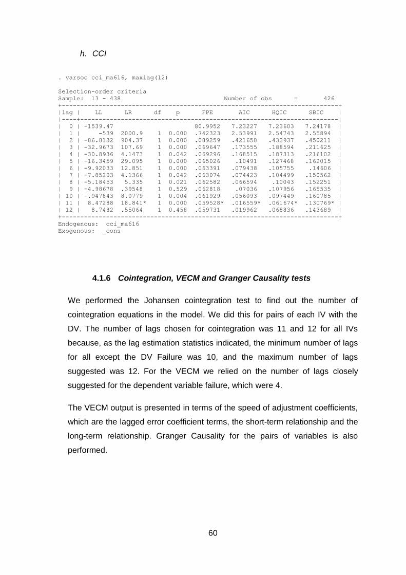
60
h. CCI
. varsoc cci_ma616, maxlag(12)
Selection-order criteria
Sample: 13 - 438 Number of obs = 426
+---------------------------------------------------------------------------+
|lag | LL LR df p FPE AIC HQIC SBIC |
|----+----------------------------------------------------------------------|
| 0 | -1539.47 80.9952 7.23227 7.23603 7.24178 |
| 1 | -539 2000.9 1 0.000 .742323 2.53991 2.54743 2.55894 |
| 2 | -86.8132 904.37 1 0.000 .089259 .421658 .432937 .450211 |
| 3 | -32.9673 107.69 1 0.000 .069647 .173555 .188594 .211625 |
| 4 | -30.8936 4.1473 1 0.042 .069296 .168515 .187313 .216102 |
| 5 | -16.3459 29.095 1 0.000 .065026 .10491 .127468 .162015 |
| 6 | -9.92033 12.851 1 0.000 .063391 .079438 .105755 .14606 |
| 7 | -7.85203 4.1366 1 0.042 .063074 .074423 .104499 .150562 |
| 8 | -5.18453 5.335 1 0.021 .062582 .066594 .10043 .152251 |
| 9 | -4.98678 .39548 1 0.529 .062818 .07036 .107956 .165535 |
| 10 | -.947843 8.0779 1 0.004 .061929 .056093 .097449 .160785 |
| 11 | 8.47288 18.841* 1 0.000 .059528* .016559* .061674* .130769* |
| 12 | 8.7482 .55064 1 0.458 .059731 .019962 .068836 .143689 |
+---------------------------------------------------------------------------+
Endogenous: cci_ma616
Exogenous: _cons
4.1.6 Cointegration, VECM and Granger Causality tests
We performed the Johansen cointegration test to find out the number of
cointegration equations in the model. We did this for pairs of each IV with the
DV. The number of lags chosen for cointegration was 11 and 12 for all IVs
because, as the lag estimation statistics indicated, the minimum number of lags
for all except the DV Failure was 10, and the maximum number of lags
suggested was 12. For the VECM we relied on the number of lags closely
suggested for the dependent variable failure, which were 4.
The VECM output is presented in terms of the speed of adjustment coefficients,
which are the lagged error coefficient terms, the short-term relationship and the
long-term relationship. Granger Causality for the pairs of variables is also
performed.
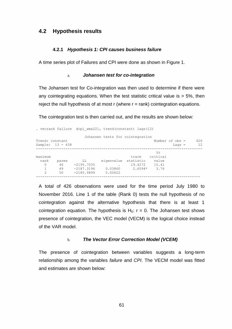
61
4.2 Hypothesis results
4.2.1 Hypothesis 1: CPI causes business failure
A time series plot of Failures and CPI were done as shown in Figure 1.
a. Johansen test for co-integration
The Johansen test for Co-integration was then used to determine if there were
any cointegrating equations. When the test statistic critical value is > 5%, then
reject the null hypothesis of at most r (where r = rank) cointegration equations.
The cointegration test is then carried out, and the results are shown below:
. vecrank failure dcpi_wma221, trend(constant) lags(12)
Johansen tests for cointegration
Trend: constant Number of obs = 426
Sample: 13 - 438 Lags = 12
-------------------------------------------------------------------------------
5%
maximum trace critical
rank parms LL eigenvalue statistic value
0 46 -2195.7035 . 19.4272 15.41
1 49 -2187.3196 0.03860 2.6594* 3.76
2 50 -2185.9899 0.00622
------------------------------------------------------------------------------
A total of 426 observations were used for the time period July 1980 to
November 2016. Line 1 of the table (Rank 0) tests the null hypothesis of no
cointegration against the alternative hypothesis that there is at least 1
cointegration equation. The hypothesis is H0: r = 0. The Johansen test shows
presence of cointegration, the VEC model (VECM) is the logical choice instead
of the VAR model.
b. The Vector Error Correction Model (VCEM)
The presence of cointegration between variables suggests a long-term
relationship among the variables failure and CPI. The VECM model was fitted
and estimates are shown below:
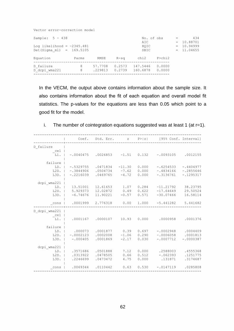
62
Vector error-correction model
Sample: 5 - 438 No. of obs = 434
AIC = 10.88701
Log likelihood = -2345.481 HQIC = 10.94999
Det(Sigma_ml) = 169.5105 SBIC = 11.04655
Equation Parms RMSE R-sq chi2 P>chi2
----------------------------------------------------------------
D_failure 8 57.7708 0.2573 147.5446 0.0000
D_dcpi_wma221 8 .229813 0.2739 160.6878 0.0000
----------------------------------------------------------------
In the VECM, the output above contains information about the sample size. It
also contains information about the fit of each equation and overall model fit
statistics. The p-values for the equations are less than 0.05 which point to a
good fit for the model.
i. The number of cointegration equations suggested was at least 1 (at r=1).
-------------------------------------------------------------------------------
| Coef. Std. Err. z P>|z| [95% Conf. Interval]
--------------+----------------------------------------------------------------
D_failure |
_ce1 |
L1. | -.0040475 .0026853 -1.51 0.132 -.0093105 .0012155
|
failure |
LD. | -.5329755 .0471834 -11.30 0.000 -.6254533 -.4404977
L2D. | -.3844906 .0504734 -7.62 0.000 -.4834166 -.2855646
L3D. | -.2216039 .0469765 -4.72 0.000 -.3136761 -.1295317
|
dcpi_wma221 |
LD. | 13.51001 12.61653 1.07 0.284 -11.21792 38.23795
L2D. | 5.929373 12.02872 0.49 0.622 -17.64649 29.50524
L3D. | -6.74676 11.90221 -0.57 0.571 -30.07466 16.58114
|
_cons | .0001999 2.776318 0.00 1.000 -5.441282 5.441682
--------------+----------------------------------------------------------------
D_dcpi_wma221 |
_ce1 |
L1. | .0001167 .0000107 10.93 0.000 .0000958 .0001376
|
failure |
LD. | .000073 .0001877 0.39 0.697 -.0002948 .0004409
L2D. | -.0002123 .0002008 -1.06 0.290 -.0006058 .0001813
L3D. | -.000405 .0001869 -2.17 0.030 -.0007712 -.0000387
|
dcpi_wma221 |
LD. | .3571686 .0501888 7.12 0.000 .2588003 .4555368
L2D. | .0313922 .0478505 0.66 0.512 -.062393 .1251775
L3D. | .2246699 .0473472 4.75 0.000 .131871 .3174687
|
_cons | .0069344 .0110442 0.63 0.530 -.0147119 .0285808
-------------------------------------------------------------------------------
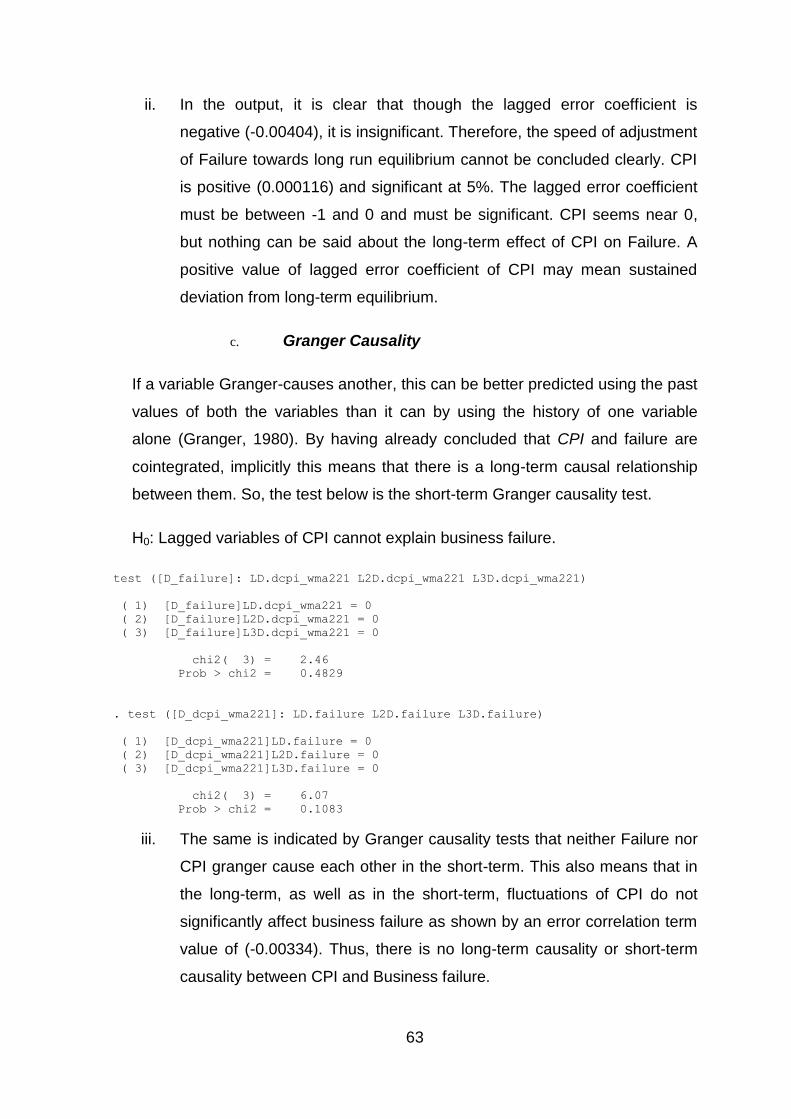
63
ii. In the output, it is clear that though the lagged error coefficient is
negative (-0.00404), it is insignificant. Therefore, the speed of adjustment
of Failure towards long run equilibrium cannot be concluded clearly. CPI
is positive (0.000116) and significant at 5%. The lagged error coefficient
must be between -1 and 0 and must be significant. CPI seems near 0,
but nothing can be said about the long-term effect of CPI on Failure. A
positive value of lagged error coefficient of CPI may mean sustained
deviation from long-term equilibrium.
c. Granger Causality
If a variable Granger-causes another, this can be better predicted using the past
values of both the variables than it can by using the history of one variable
alone (Granger, 1980). By having already concluded that CPI and failure are
cointegrated, implicitly this means that there is a long-term causal relationship
between them. So, the test below is the short-term Granger causality test.
H0: Lagged variables of CPI cannot explain business failure.
test ([D_failure]: LD.dcpi_wma221 L2D.dcpi_wma221 L3D.dcpi_wma221)
( 1) [D_failure]LD.dcpi_wma221 = 0
( 2) [D_failure]L2D.dcpi_wma221 = 0
( 3) [D_failure]L3D.dcpi_wma221 = 0
chi2( 3) = 2.46
Prob > chi2 = 0.4829
. test ([D_dcpi_wma221]: LD.failure L2D.failure L3D.failure)
( 1) [D_dcpi_wma221]LD.failure = 0
( 2) [D_dcpi_wma221]L2D.failure = 0
( 3) [D_dcpi_wma221]L3D.failure = 0
chi2( 3) = 6.07
Prob > chi2 = 0.1083
iii. The same is indicated by Granger causality tests that neither Failure nor
CPI granger cause each other in the short-term. This also means that in
the long-term, as well as in the short-term, fluctuations of CPI do not
significantly affect business failure as shown by an error correlation term
value of (-0.00334). Thus, there is no long-term causality or short-term
causality between CPI and Business failure.
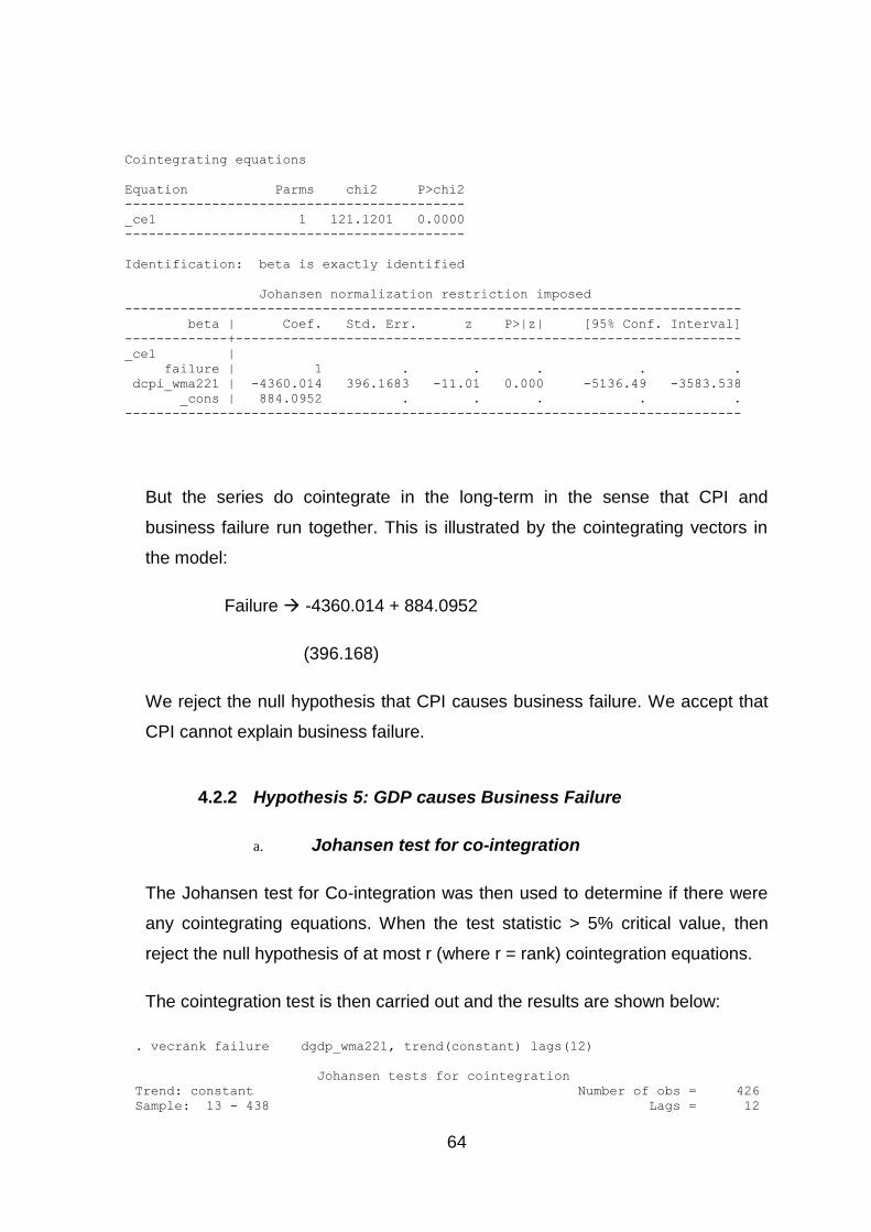
64
Cointegrating equations
Equation Parms chi2 P>chi2
-------------------------------------------
_ce1 1 121.1201 0.0000
-------------------------------------------
Identification: beta is exactly identified
Johansen normalization restriction imposed
------------------------------------------------------------------------------
beta | Coef. Std. Err. z P>|z| [95% Conf. Interval]
-------------+----------------------------------------------------------------
_ce1 |
failure | 1 . . . . .
dcpi_wma221 | -4360.014 396.1683 -11.01 0.000 -5136.49 -3583.538
_cons | 884.0952 . . . . .
------------------------------------------------------------------------------
But the series do cointegrate in the long-term in the sense that CPI and
business failure run together. This is illustrated by the cointegrating vectors in
the model:
Failure -4360.014 + 884.0952
(396.168)
We reject the null hypothesis that CPI causes business failure. We accept that
CPI cannot explain business failure.
4.2.2 Hypothesis 5: GDP causes Business Failure
a. Johansen test for co-integration
The Johansen test for Co-integration was then used to determine if there were
any cointegrating equations. When the test statistic > 5% critical value, then
reject the null hypothesis of at most r (where r = rank) cointegration equations.
The cointegration test is then carried out and the results are shown below:
. vecrank failure dgdp_wma221, trend(constant) lags(12)
Johansen tests for cointegration
Trend: constant Number of obs = 426
Sample: 13 - 438 Lags = 12
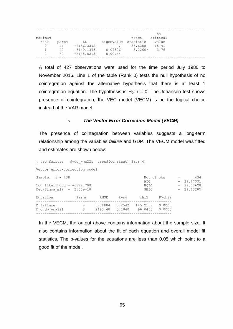
65
-------------------------------------------------------------------------------
5%
maximum trace critical
rank parms LL eigenvalue statistic value
0 46 -6156.3392 . 35.6358 15.41
1 49 -6140.1343 0.07326 3.2260* 3.76
2 50 -6138.5213 0.00754
-------------------------------------------------------------------------------
A total of 427 observations were used for the time period July 1980 to
November 2016. Line 1 of the table (Rank 0) tests the null hypothesis of no
cointegration against the alternative hypothesis that there is at least 1
cointegration equation. The hypothesis is H0: r = 0. The Johansen test shows
presence of cointegration, the VEC model (VECM) is be the logical choice
instead of the VAR model.
b. The Vector Error Correction Model (VECM)
The presence of cointegration between variables suggests a long-term
relationship among the variables failure and GDP. The VECM model was fitted
and estimates are shown below:
. vec failure dgdp_wma221, trend(constant) lags(4)
Vector error-correction model
Sample: 5 - 438 No. of obs = 434
AIC = 29.47331
Log likelihood = -6378.708 HQIC = 29.53628
Det(Sigma_ml) = 2.00e+10 SBIC = 29.63285
Equation Parms RMSE R-sq chi2 P>chi2
----------------------------------------------------------------
D_failure 8 57.8884 0.2542 145.2158 0.0000
D_dgdp_wma221 8 2493.48 0.1840 96.0435 0.0000
----------------------------------------------------------------
In the VECM, the output above contains information about the sample size. It
also contains information about the fit of each equation and overall model fit
statistics. The p-values for the equations are less than 0.05 which point to a
good fit of the model.
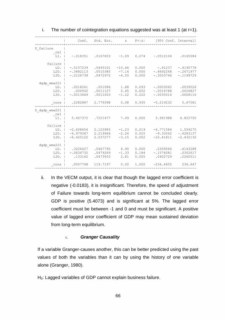
66
i. The number of cointegration equations suggested was at least 1 (at r=1).
-------------------------------------------------------------------------------
| Coef. Std. Err. z P>|z| [95% Conf. Interval]
--------------+----------------------------------------------------------------
D_failure |
_ce1 |
L1. | -.018351 .0167653 -1.09 0.274 -.0512104 .0145084
|
failure |
LD. | -.5157239 .0493101 -10.46 0.000 -.61237 -.4190778
L2D. | -.3682113 .0515385 -7.14 0.000 -.4692248 -.2671977
L3D. | -.2126738 .0472972 -4.50 0.000 -.3053746 -.1199729
|
dgdp_wma221 |
LD. | .0018241 .001086 1.68 0.093 -.0003045 .0039526
L2D. | .000502 .0011127 0.45 0.652 -.0016788 .0026827
L3D. | -.0013449 .0011003 -1.22 0.222 -.0035014 .0008116
|
_cons | .2282887 2.779398 0.08 0.935 -5.219232 5.67581
--------------+----------------------------------------------------------------
D_dgdp_wma221 |
_ce1 |
L1. | 5.407372 .7221477 7.49 0.000 3.991988 6.822755
|
failure |
LD. | -2.608654 2.123983 -1.23 0.219 -6.771584 1.554275
L2D. | -4.979367 2.219966 -2.24 0.025 -9.33042 -.6283137
L3D. | -6.425122 2.037277 -3.15 0.002 -10.41811 -2.432132
|
dgdp_wma221 |
LD. | .3226427 .0467795 6.90 0.000 .2309566 .4143288
L2D. | -.0636732 .0479269 -1.33 0.184 -.1576081 .0302617
L3D. | .133162 .0473933 2.81 0.005 .0402729 .2260511
|
_cons | .0007748 119.7197 0.00 1.000 -234.6455 234.647
-------------------------------------------------------------------------------
ii. In the VECM output, it is clear that though the lagged error coefficient is
negative (-0.0183), it is insignificant. Therefore, the speed of adjustment
of Failure towards long-term equilibrium cannot be concluded clearly.
GDP is positive (5.4073) and is significant at 5%. The lagged error
coefficient must be between -1 and 0 and must be significant. A positive
value of lagged error coefficient of GDP may mean sustained deviation
from long-term equilibrium.
c. Granger Causality
If a variable Granger-causes another, this can be better predicted using the past
values of both the variables than it can by using the history of one variable
alone (Granger, 1980).
H0: Lagged variables of GDP cannot explain business failure.
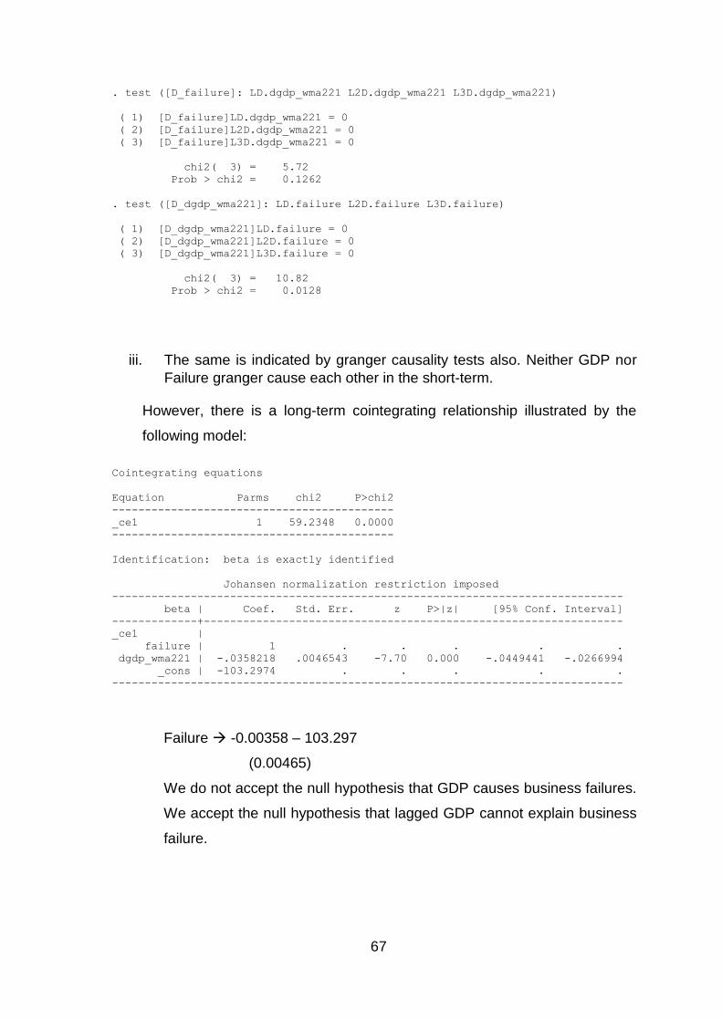
67
. test ([D_failure]: LD.dgdp_wma221 L2D.dgdp_wma221 L3D.dgdp_wma221)
( 1) [D_failure]LD.dgdp_wma221 = 0
( 2) [D_failure]L2D.dgdp_wma221 = 0
( 3) [D_failure]L3D.dgdp_wma221 = 0
chi2( 3) = 5.72
Prob > chi2 = 0.1262
. test ([D_dgdp_wma221]: LD.failure L2D.failure L3D.failure)
( 1) [D_dgdp_wma221]LD.failure = 0
( 2) [D_dgdp_wma221]L2D.failure = 0
( 3) [D_dgdp_wma221]L3D.failure = 0
chi2( 3) = 10.82
Prob > chi2 = 0.0128
iii. The same is indicated by granger causality tests also. Neither GDP nor
Failure granger cause each other in the short-term.
However, there is a long-term cointegrating relationship illustrated by the
following model:
Cointegrating equations
Equation Parms chi2 P>chi2
-------------------------------------------
_ce1 1 59.2348 0.0000
-------------------------------------------
Identification: beta is exactly identified
Johansen normalization restriction imposed
------------------------------------------------------------------------------
beta | Coef. Std. Err. z P>|z| [95% Conf. Interval]
-------------+----------------------------------------------------------------
_ce1 |
failure | 1 . . . . .
dgdp_wma221 | -.0358218 .0046543 -7.70 0.000 -.0449441 -.0266994
_cons | -103.2974 . . . . .
------------------------------------------------------------------------------
Failure -0.00358 – 103.297
(0.00465)
We do not accept the null hypothesis that GDP causes business failures.
We accept the null hypothesis that lagged GDP cannot explain business
failure.
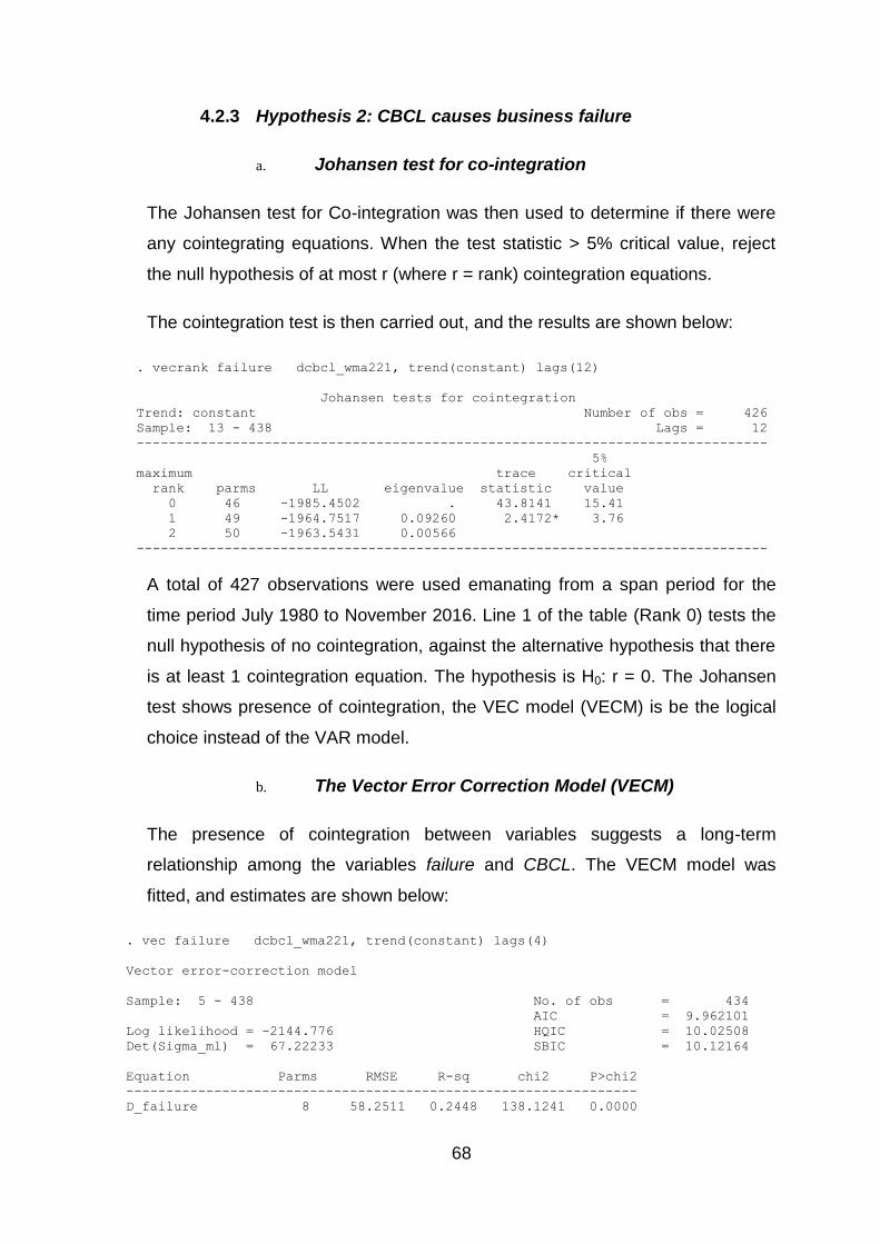
68
4.2.3 Hypothesis 2: CBCL causes business failure
a. Johansen test for co-integration
The Johansen test for Co-integration was then used to determine if there were
any cointegrating equations. When the test statistic > 5% critical value, reject
the null hypothesis of at most r (where r = rank) cointegration equations.
The cointegration test is then carried out, and the results are shown below:
. vecrank failure dcbcl_wma221, trend(constant) lags(12)
Johansen tests for cointegration
Trend: constant Number of obs = 426
Sample: 13 - 438 Lags = 12
-------------------------------------------------------------------------------
5%
maximum trace critical
rank parms LL eigenvalue statistic value
0 46 -1985.4502 . 43.8141 15.41
1 49 -1964.7517 0.09260 2.4172* 3.76
2 50 -1963.5431 0.00566
-------------------------------------------------------------------------------
A total of 427 observations were used emanating from a span period for the
time period July 1980 to November 2016. Line 1 of the table (Rank 0) tests the
null hypothesis of no cointegration, against the alternative hypothesis that there
is at least 1 cointegration equation. The hypothesis is H0: r = 0. The Johansen
test shows presence of cointegration, the VEC model (VECM) is be the logical
choice instead of the VAR model.
b. The Vector Error Correction Model (VECM)
The presence of cointegration between variables suggests a long-term
relationship among the variables failure and CBCL. The VECM model was
fitted, and estimates are shown below:
. vec failure dcbcl_wma221, trend(constant) lags(4)
Vector error-correction model
Sample: 5 - 438 No. of obs = 434
AIC = 9.962101
Log likelihood = -2144.776 HQIC = 10.02508
Det(Sigma_ml) = 67.22233 SBIC = 10.12164
Equation Parms RMSE R-sq chi2 P>chi2
----------------------------------------------------------------
D_failure 8 58.2511 0.2448 138.1241 0.0000
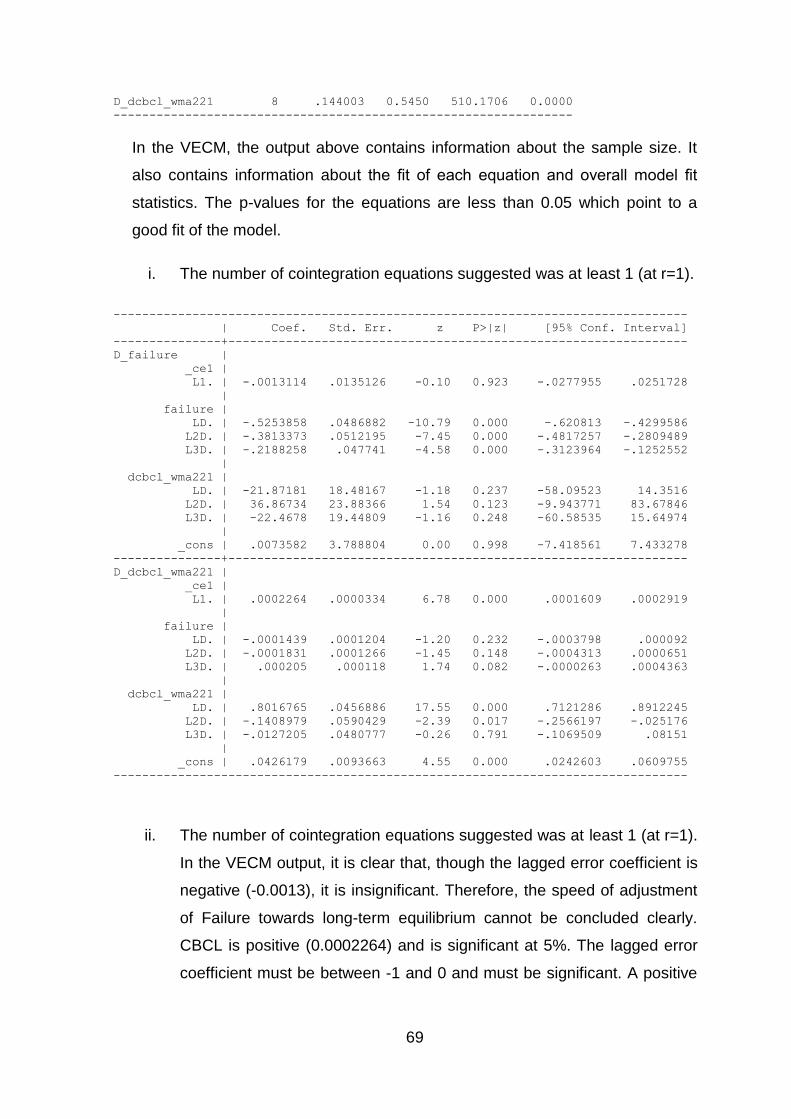
69
D_dcbcl_wma221 8 .144003 0.5450 510.1706 0.0000
----------------------------------------------------------------
In the VECM, the output above contains information about the sample size. It
also contains information about the fit of each equation and overall model fit
statistics. The p-values for the equations are less than 0.05 which point to a
good fit of the model.
i. The number of cointegration equations suggested was at least 1 (at r=1).
--------------------------------------------------------------------------------
| Coef. Std. Err. z P>|z| [95% Conf. Interval]
---------------+----------------------------------------------------------------
D_failure |
_ce1 |
L1. | -.0013114 .0135126 -0.10 0.923 -.0277955 .0251728
|
failure |
LD. | -.5253858 .0486882 -10.79 0.000 -.620813 -.4299586
L2D. | -.3813373 .0512195 -7.45 0.000 -.4817257 -.2809489
L3D. | -.2188258 .047741 -4.58 0.000 -.3123964 -.1252552
|
dcbcl_wma221 |
LD. | -21.87181 18.48167 -1.18 0.237 -58.09523 14.3516
L2D. | 36.86734 23.88366 1.54 0.123 -9.943771 83.67846
L3D. | -22.4678 19.44809 -1.16 0.248 -60.58535 15.64974
|
_cons | .0073582 3.788804 0.00 0.998 -7.418561 7.433278
---------------+----------------------------------------------------------------
D_dcbcl_wma221 |
_ce1 |
L1. | .0002264 .0000334 6.78 0.000 .0001609 .0002919
|
failure |
LD. | -.0001439 .0001204 -1.20 0.232 -.0003798 .000092
L2D. | -.0001831 .0001266 -1.45 0.148 -.0004313 .0000651
L3D. | .000205 .000118 1.74 0.082 -.0000263 .0004363
|
dcbcl_wma221 |
LD. | .8016765 .0456886 17.55 0.000 .7121286 .8912245
L2D. | -.1408979 .0590429 -2.39 0.017 -.2566197 -.025176
L3D. | -.0127205 .0480777 -0.26 0.791 -.1069509 .08151
|
_cons | .0426179 .0093663 4.55 0.000 .0242603 .0609755
--------------------------------------------------------------------------------
ii. The number of cointegration equations suggested was at least 1 (at r=1).
In the VECM output, it is clear that, though the lagged error coefficient is
negative (-0.0013), it is insignificant. Therefore, the speed of adjustment
of Failure towards long-term equilibrium cannot be concluded clearly.
CBCL is positive (0.0002264) and is significant at 5%. The lagged error
coefficient must be between -1 and 0 and must be significant. A positive
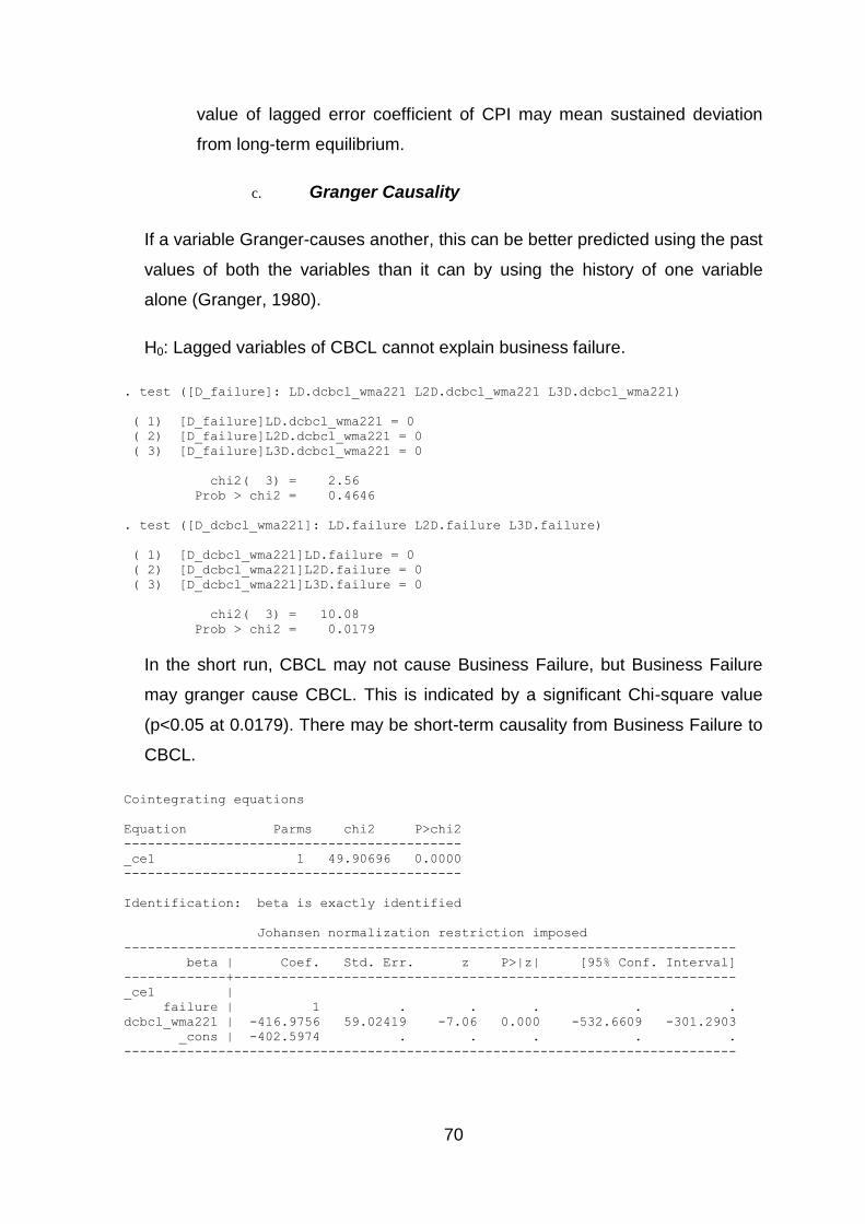
70
value of lagged error coefficient of CPI may mean sustained deviation
from long-term equilibrium.
c. Granger Causality
If a variable Granger-causes another, this can be better predicted using the past
values of both the variables than it can by using the history of one variable
alone (Granger, 1980).
H0: Lagged variables of CBCL cannot explain business failure.
. test ([D_failure]: LD.dcbcl_wma221 L2D.dcbcl_wma221 L3D.dcbcl_wma221)
( 1) [D_failure]LD.dcbcl_wma221 = 0
( 2) [D_failure]L2D.dcbcl_wma221 = 0
( 3) [D_failure]L3D.dcbcl_wma221 = 0
chi2( 3) = 2.56
Prob > chi2 = 0.4646
. test ([D_dcbcl_wma221]: LD.failure L2D.failure L3D.failure)
( 1) [D_dcbcl_wma221]LD.failure = 0
( 2) [D_dcbcl_wma221]L2D.failure = 0
( 3) [D_dcbcl_wma221]L3D.failure = 0
chi2( 3) = 10.08
Prob > chi2 = 0.0179
In the short run, CBCL may not cause Business Failure, but Business Failure
may granger cause CBCL. This is indicated by a significant Chi-square value
(p<0.05 at 0.0179). There may be short-term causality from Business Failure to
CBCL.
Cointegrating equations
Equation Parms chi2 P>chi2
-------------------------------------------
_ce1 1 49.90696 0.0000
-------------------------------------------
Identification: beta is exactly identified
Johansen normalization restriction imposed
------------------------------------------------------------------------------
beta | Coef. Std. Err. z P>|z| [95% Conf. Interval]
-------------+----------------------------------------------------------------
_ce1 |
failure | 1 . . . . .
dcbcl_wma221 | -416.9756 59.02419 -7.06 0.000 -532.6609 -301.2903
_cons | -402.5974 . . . . .
------------------------------------------------------------------------------
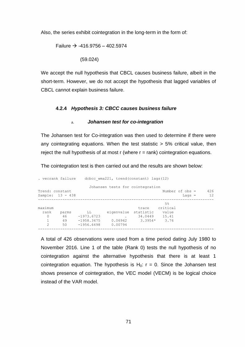
71
Also, the series exhibit cointegration in the long-term in the form of:
Failure -416.9756 – 402.5974
(59.024)
We accept the null hypothesis that CBCL causes business failure, albeit in the
short-term. However, we do not accept the hypothesis that lagged variables of
CBCL cannot explain business failure.
4.2.4 Hypothesis 3: CBCC causes business failure
a. Johansen test for co-integration
The Johansen test for Co-integration was then used to determine if there were
any cointegrating equations. When the test statistic > 5% critical value, then
reject the null hypothesis of at most r (where r = rank) cointegration equations.
The cointegration test is then carried out and the results are shown below:
. vecrank failure dcbcc_wma221, trend(constant) lags(12)
Johansen tests for cointegration
Trend: constant Number of obs = 426
Sample: 13 - 438 Lags = 12
-------------------------------------------------------------------------------
5%
maximum trace critical
rank parms LL eigenvalue statistic value
0 46 -1973.6723 . 34.0449 15.41
1 49 -1958.3475 0.06942 3.3954* 3.76
2 50 -1956.6498 0.00794
-------------------------------------------------------------------------------
A total of 426 observations were used from a time period dating July 1980 to
November 2016. Line 1 of the table (Rank 0) tests the null hypothesis of no
cointegration against the alternative hypothesis that there is at least 1
cointegration equation. The hypothesis is H0: r = 0. Since the Johansen test
shows presence of cointegration, the VEC model (VECM) is be logical choice
instead of the VAR model.
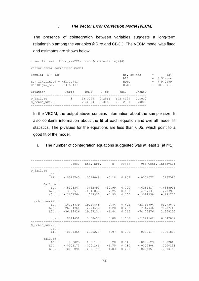
72
b. The Vector Error Correction Model (VECM)
The presence of cointegration between variables suggests a long-term
relationship among the variables failure and CBCC. The VECM model was fitted
and estimates are shown below:
. vec failure dcbcc_wma221, trend(constant) lags(4)
Vector error-correction model
Sample: 5 - 438 No. of obs = 434
AIC = 9.907564
Log likelihood = -2132.941 HQIC = 9.970539
Det(Sigma_ml) = 63.65444 SBIC = 10.06711
Equation Parms RMSE R-sq chi2 P>chi2
----------------------------------------------------------------
D_failure 8 58.0095 0.2511 142.8329 0.0000
D_dcbcc_wma221 8 .140904 0.3469 226.2351 0.0000
----------------------------------------------------------------
In the VECM, the output above contains information about the sample size. It
also contains information about the fit of each equation and overall model fit
statistics. The p-values for the equations are less than 0.05, which point to a
good fit of the model.
i. The number of cointegration equations suggested was at least 1 (at r=1).
--------------------------------------------------------------------------------
| Coef. Std. Err. z P>|z| [95% Conf. Interval]
---------------+----------------------------------------------------------------
D_failure |
_ce1 |
L1. | -.0016745 .0094049 -0.18 0.859 -.0201077 .0167587
|
failure |
LD. | -.5305367 .0482892 -10.99 0.000 -.6251817 -.4358916
L2D. | -.3705517 .0511037 -7.25 0.000 -.4707131 -.2703903
L3D. | -.2154764 .047322 -4.55 0.000 -.3082259 -.122727
|
dcbcc_wma221 |
LD. | 16.08839 19.20868 0.84 0.402 -21.55994 53.73672
L2D. | 26.84761 22.4632 1.20 0.232 -17.17946 70.87468
L3D. | -36.19826 19.67204 -1.84 0.066 -74.75476 2.358235
|
_cons | .0014651 3.08455 0.00 1.000 -6.044142 6.047072
---------------+----------------------------------------------------------------
D_dcbcc_wma221 |
_ce1 |
L1. | .0001365 .0000228 5.97 0.000 .0000917 .0001812
|
failure |
LD. | -.000023 .0001173 -0.20 0.845 -.0002529 .0002069
L2D. | -.0002175 .0001241 -1.75 0.080 -.0004608 .0000258
L3D. | -.0002098 .0001149 -1.83 0.068 -.0004351 .0000155
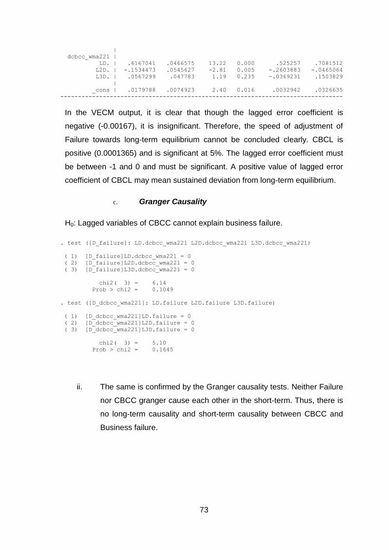
73
|
dcbcc_wma221 |
LD. | .6167041 .0466575 13.22 0.000 .525257 .7081512
L2D. | -.1534473 .0545627 -2.81 0.005 -.2603883 -.0465064
L3D. | .0567299 .047783 1.19 0.235 -.0369231 .1503829
|
_cons | .0179788 .0074923 2.40 0.016 .0032942 .0326635
--------------------------------------------------------------------------------
In the VECM output, it is clear that though the lagged error coefficient is
negative (-0.00167), it is insignificant. Therefore, the speed of adjustment of
Failure towards long-term equilibrium cannot be concluded clearly. CBCL is
positive (0.0001365) and is significant at 5%. The lagged error coefficient must
be between -1 and 0 and must be significant. A positive value of lagged error
coefficient of CBCL may mean sustained deviation from long-term equilibrium.
c. Granger Causality
H0: Lagged variables of CBCC cannot explain business failure.
. test ([D_failure]: LD.dcbcc_wma221 L2D.dcbcc_wma221 L3D.dcbcc_wma221)
( 1) [D_failure]LD.dcbcc_wma221 = 0
( 2) [D_failure]L2D.dcbcc_wma221 = 0
( 3) [D_failure]L3D.dcbcc_wma221 = 0
chi2( 3) = 6.14
Prob > chi2 = 0.1049
. test ([D_dcbcc_wma221]: LD.failure L2D.failure L3D.failure)
( 1) [D_dcbcc_wma221]LD.failure = 0
( 2) [D_dcbcc_wma221]L2D.failure = 0
( 3) [D_dcbcc_wma221]L3D.failure = 0
chi2( 3) = 5.10
Prob > chi2 = 0.1645
ii. The same is confirmed by the Granger causality tests. Neither Failure
nor CBCC granger cause each other in the short-term. Thus, there is
no long-term causality and short-term causality between CBCC and
Business failure.
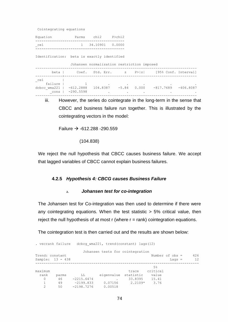
74
Cointegrating equations
Equation Parms chi2 P>chi2
-------------------------------------------
_ce1 1 34.10901 0.0000
-------------------------------------------
Identification: beta is exactly identified
Johansen normalization restriction imposed
------------------------------------------------------------------------------
beta | Coef. Std. Err. z P>|z| [95% Conf. Interval]
-------------+----------------------------------------------------------------
_ce1 |
failure | 1 . . . . .
dcbcc_wma221 | -612.2888 104.8387 -5.84 0.000 -817.7689 -406.8087
_cons | -290.5598 . . . . .
------------------------------------------------------------------------------
iii. However, the series do cointegrate in the long-term in the sense that
CBCC and business failure run together. This is illustrated by the
cointegrating vectors in the model:
Failure -612.288 -290.559
(104.838)
We reject the null hypothesis that CBCC causes business failure. We accept
that lagged variables of CBCC cannot explain business failures.
4.2.5 Hypothesis 4: CBCG causes Business Failure
a. Johansen test for co-integration
The Johansen test for Co-integration was then used to determine if there were
any cointegrating equations. When the test statistic > 5% critical value, then
reject the null hypothesis of at most r (where r = rank) cointegration equations.
The cointegration test is then carried out and the results are shown below:
. vecrank failure dcbcg_wma221, trend(constant) lags(12)
Johansen tests for cointegration
Trend: constant Number of obs = 426
Sample: 13 - 438 Lags = 12
-------------------------------------------------------------------------------
5%
maximum trace critical
rank parms LL eigenvalue statistic value
0 46 -2215.6474 . 33.8395 15.41
1 49 -2199.833 0.07156 2.2109* 3.76
2 50 -2198.7276 0.00518
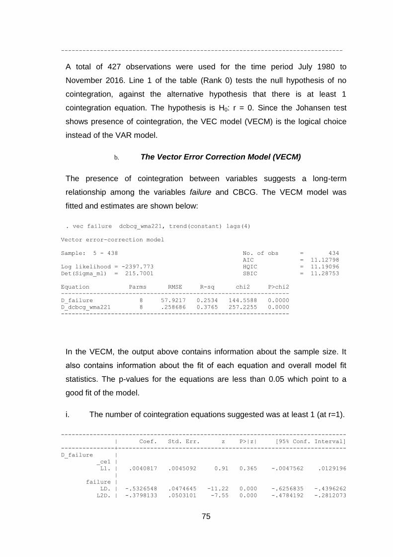
75
-------------------------------------------------------------------------------
A total of 427 observations were used for the time period July 1980 to
November 2016. Line 1 of the table (Rank 0) tests the null hypothesis of no
cointegration, against the alternative hypothesis that there is at least 1
cointegration equation. The hypothesis is H0: r = 0. Since the Johansen test
shows presence of cointegration, the VEC model (VECM) is the logical choice
instead of the VAR model.
b. The Vector Error Correction Model (VECM)
The presence of cointegration between variables suggests a long-term
relationship among the variables failure and CBCG. The VECM model was
fitted and estimates are shown below:
. vec failure dcbcg_wma221, trend(constant) lags(4)
Vector error-correction model
Sample: 5 - 438 No. of obs = 434
AIC = 11.12798
Log likelihood = -2397.773 HQIC = 11.19096
Det(Sigma_ml) = 215.7001 SBIC = 11.28753
Equation Parms RMSE R-sq chi2 P>chi2
----------------------------------------------------------------
D_failure 8 57.9217 0.2534 144.5588 0.0000
D_dcbcg_wma221 8 .258686 0.3765 257.2255 0.0000
----------------------------------------------------------------
In the VECM, the output above contains information about the sample size. It
also contains information about the fit of each equation and overall model fit
statistics. The p-values for the equations are less than 0.05 which point to a
good fit of the model.
i. The number of cointegration equations suggested was at least 1 (at r=1).
--------------------------------------------------------------------------------
| Coef. Std. Err. z P>|z| [95% Conf. Interval]
---------------+----------------------------------------------------------------
D_failure |
_ce1 |
L1. | .0040817 .0045092 0.91 0.365 -.0047562 .0129196
|
failure |
LD. | -.5326548 .0474645 -11.22 0.000 -.6256835 -.4396262
L2D. | -.3798133 .0503101 -7.55 0.000 -.4784192 -.2812073
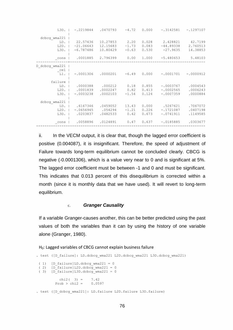
76
L3D. | -.2219844 .0470793 -4.72 0.000 -.3142581 -.1297107
|
dcbcg_wma221 |
LD. | 22.57436 10.27853 2.20 0.028 2.428821 42.7199
L2D. | -21.06643 12.15683 -1.73 0.083 -44.89338 2.760513
L3D. | -6.787486 10.80429 -0.63 0.530 -27.9635 14.38853
|
_cons | .0001885 2.796399 0.00 1.000 -5.480653 5.48103
---------------+----------------------------------------------------------------
D_dcbcg_wma221 |
_ce1 |
L1. | -.0001306 .0000201 -6.49 0.000 -.0001701 -.0000912
|
failure |
LD. | .0000388 .000212 0.18 0.855 -.0003767 .0004543
L2D. | .0001839 .0002247 0.82 0.413 -.0002565 .0006243
L3D. | -.0003238 .0002103 -1.54 0.124 -.0007359 .0000884
|
dcbcg_wma221 |
LD. | .6167346 .0459052 13.43 0.000 .5267621 .7067072
L2D. | -.0656945 .054294 -1.21 0.226 -.1721087 .0407198
L3D. | .0203837 .0482533 0.42 0.673 -.0741911 .1149585
|
_cons | .0058896 .0124891 0.47 0.637 -.0185885 .0303677
--------------------------------------------------------------------------------
ii. In the VECM output, it is clear that, though the lagged error coefficient is
positive (0.004087), it is insignificant. Therefore, the speed of adjustment of
Failure towards long-term equilibrium cannot be concluded clearly. CBCG is
negative (-0.0001306), which is a value very near to 0 and is significant at 5%.
The lagged error coefficient must be between -1 and 0 and must be significant.
This indicates that 0.013 percent of this disequilibrium is corrected within a
month (since it is monthly data that we have used). It will revert to long-term
equilibrium.
c. Granger Causality
If a variable Granger-causes another, this can be better predicted using the past
values of both the variables than it can by using the history of one variable
alone (Granger, 1980).
H0: Lagged variables of CBCG cannot explain business failure
. test ([D_failure]: LD.dcbcg_wma221 L2D.dcbcg_wma221 L3D.dcbcg_wma221)
( 1) [D_failure]LD.dcbcg_wma221 = 0
( 2) [D_failure]L2D.dcbcg_wma221 = 0
( 3) [D_failure]L3D.dcbcg_wma221 = 0
chi2( 3) = 7.42
Prob > chi2 = 0.0597
. test ([D_dcbcg_wma221]: LD.failure L2D.failure L3D.failure)
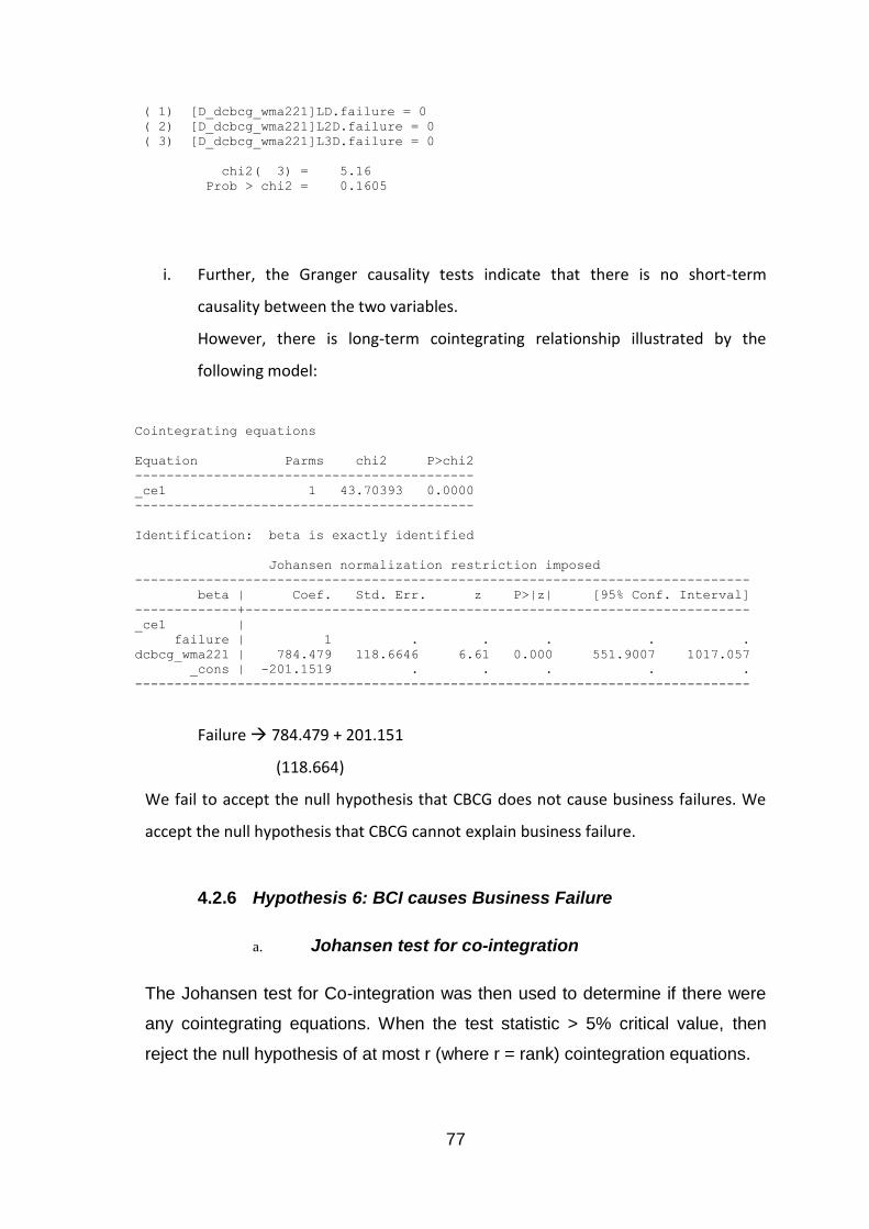
77
( 1) [D_dcbcg_wma221]LD.failure = 0
( 2) [D_dcbcg_wma221]L2D.failure = 0
( 3) [D_dcbcg_wma221]L3D.failure = 0
chi2( 3) = 5.16
Prob > chi2 = 0.1605
i. Further, the Granger causality tests indicate that there is no short-term
causality between the two variables.
However, there is long-term cointegrating relationship illustrated by the
following model:
Cointegrating equations
Equation Parms chi2 P>chi2
-------------------------------------------
_ce1 1 43.70393 0.0000
-------------------------------------------
Identification: beta is exactly identified
Johansen normalization restriction imposed
------------------------------------------------------------------------------
beta | Coef. Std. Err. z P>|z| [95% Conf. Interval]
-------------+----------------------------------------------------------------
_ce1 |
failure | 1 . . . . .
dcbcg_wma221 | 784.479 118.6646 6.61 0.000 551.9007 1017.057
_cons | -201.1519 . . . . .
------------------------------------------------------------------------------
Failure 784.479 + 201.151
(118.664)
We fail to accept the null hypothesis that CBCG does not cause business failures. We
accept the null hypothesis that CBCG cannot explain business failure.
4.2.6 Hypothesis 6: BCI causes Business Failure
a. Johansen test for co-integration
The Johansen test for Co-integration was then used to determine if there were
any cointegrating equations. When the test statistic > 5% critical value, then
reject the null hypothesis of at most r (where r = rank) cointegration equations.
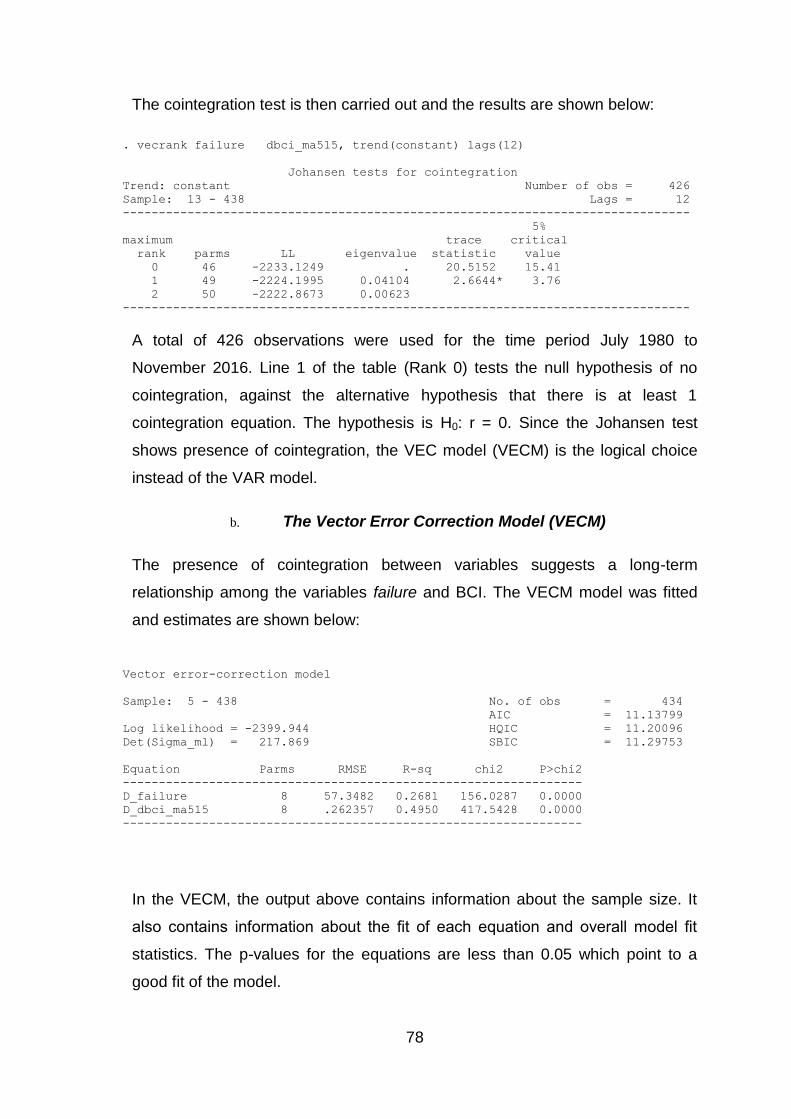
78
The cointegration test is then carried out and the results are shown below:
. vecrank failure dbci_ma515, trend(constant) lags(12)
Johansen tests for cointegration
Trend: constant Number of obs = 426
Sample: 13 - 438 Lags = 12
-------------------------------------------------------------------------------
5%
maximum trace critical
rank parms LL eigenvalue statistic value
0 46 -2233.1249 . 20.5152 15.41
1 49 -2224.1995 0.04104 2.6644* 3.76
2 50 -2222.8673 0.00623
-------------------------------------------------------------------------------
A total of 426 observations were used for the time period July 1980 to
November 2016. Line 1 of the table (Rank 0) tests the null hypothesis of no
cointegration, against the alternative hypothesis that there is at least 1
cointegration equation. The hypothesis is H0: r = 0. Since the Johansen test
shows presence of cointegration, the VEC model (VECM) is the logical choice
instead of the VAR model.
b. The Vector Error Correction Model (VECM)
The presence of cointegration between variables suggests a long-term
relationship among the variables failure and BCI. The VECM model was fitted
and estimates are shown below:
Vector error-correction model
Sample: 5 - 438 No. of obs = 434
AIC = 11.13799
Log likelihood = -2399.944 HQIC = 11.20096
Det(Sigma_ml) = 217.869 SBIC = 11.29753
Equation Parms RMSE R-sq chi2 P>chi2
----------------------------------------------------------------
D_failure 8 57.3482 0.2681 156.0287 0.0000
D_dbci_ma515 8 .262357 0.4950 417.5428 0.0000
----------------------------------------------------------------
In the VECM, the output above contains information about the sample size. It
also contains information about the fit of each equation and overall model fit
statistics. The p-values for the equations are less than 0.05 which point to a
good fit of the model.
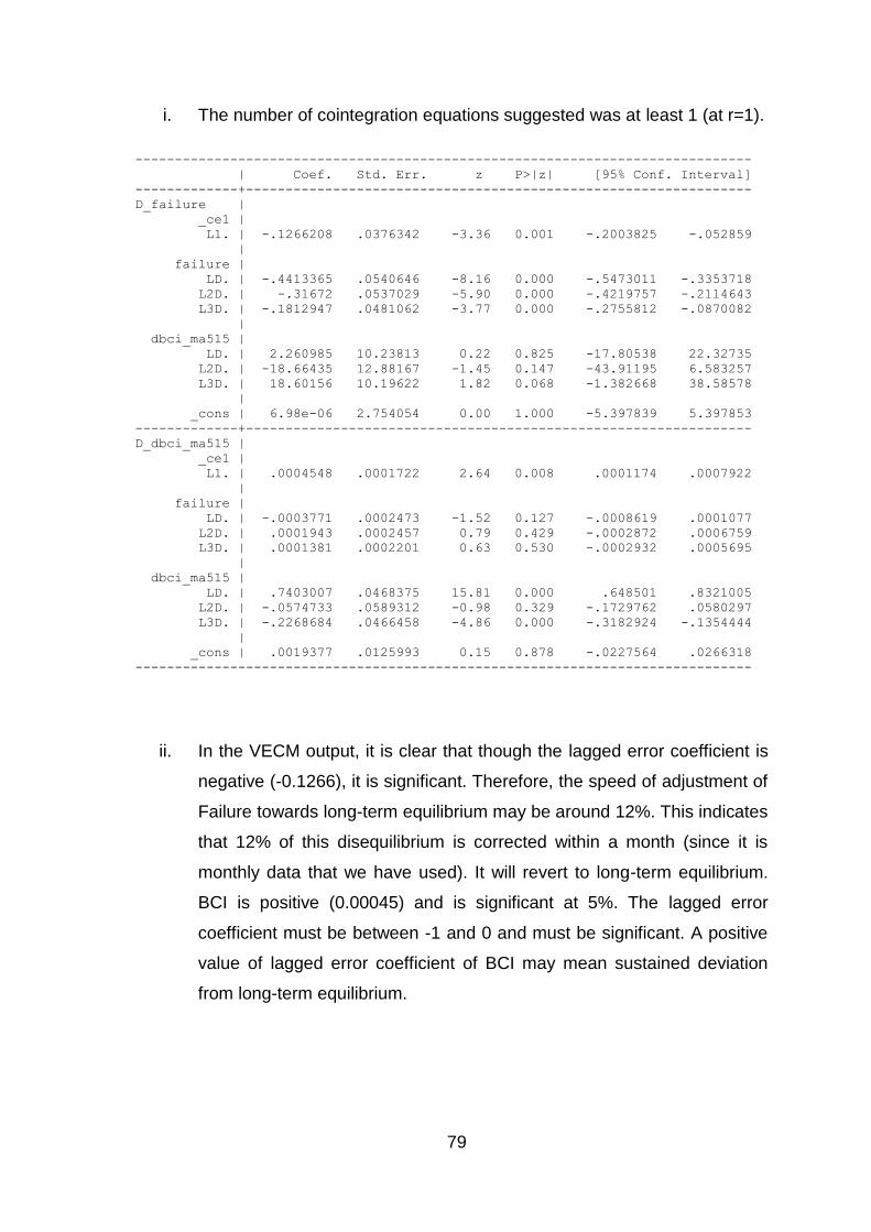
79
i. The number of cointegration equations suggested was at least 1 (at r=1).
------------------------------------------------------------------------------
| Coef. Std. Err. z P>|z| [95% Conf. Interval]
-------------+----------------------------------------------------------------
D_failure |
_ce1 |
L1. | -.1266208 .0376342 -3.36 0.001 -.2003825 -.052859
|
failure |
LD. | -.4413365 .0540646 -8.16 0.000 -.5473011 -.3353718
L2D. | -.31672 .0537029 -5.90 0.000 -.4219757 -.2114643
L3D. | -.1812947 .0481062 -3.77 0.000 -.2755812 -.0870082
|
dbci_ma515 |
LD. | 2.260985 10.23813 0.22 0.825 -17.80538 22.32735
L2D. | -18.66435 12.88167 -1.45 0.147 -43.91195 6.583257
L3D. | 18.60156 10.19622 1.82 0.068 -1.382668 38.58578
|
_cons | 6.98e-06 2.754054 0.00 1.000 -5.397839 5.397853
-------------+----------------------------------------------------------------
D_dbci_ma515 |
_ce1 |
L1. | .0004548 .0001722 2.64 0.008 .0001174 .0007922
|
failure |
LD. | -.0003771 .0002473 -1.52 0.127 -.0008619 .0001077
L2D. | .0001943 .0002457 0.79 0.429 -.0002872 .0006759
L3D. | .0001381 .0002201 0.63 0.530 -.0002932 .0005695
|
dbci_ma515 |
LD. | .7403007 .0468375 15.81 0.000 .648501 .8321005
L2D. | -.0574733 .0589312 -0.98 0.329 -.1729762 .0580297
L3D. | -.2268684 .0466458 -4.86 0.000 -.3182924 -.1354444
|
_cons | .0019377 .0125993 0.15 0.878 -.0227564 .0266318
------------------------------------------------------------------------------
ii. In the VECM output, it is clear that though the lagged error coefficient is
negative (-0.1266), it is significant. Therefore, the speed of adjustment of
Failure towards long-term equilibrium may be around 12%. This indicates
that 12% of this disequilibrium is corrected within a month (since it is
monthly data that we have used). It will revert to long-term equilibrium.
BCI is positive (0.00045) and is significant at 5%. The lagged error
coefficient must be between -1 and 0 and must be significant. A positive
value of lagged error coefficient of BCI may mean sustained deviation
from long-term equilibrium.
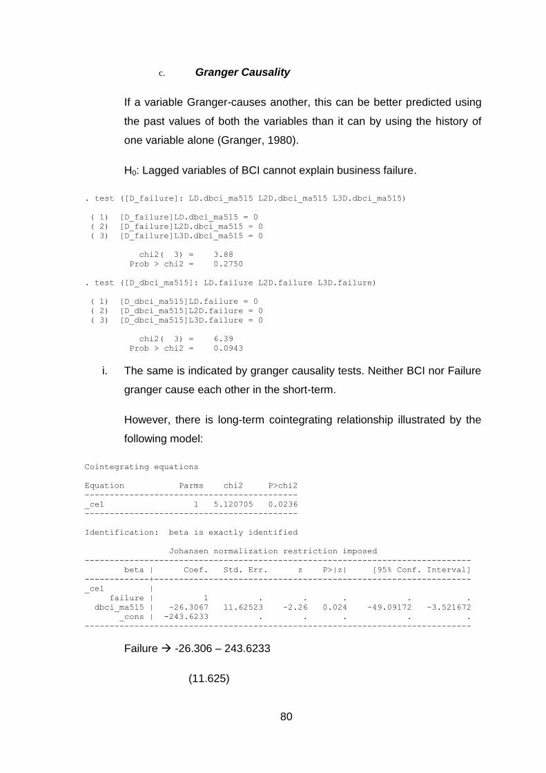
80
c. Granger Causality
If a variable Granger-causes another, this can be better predicted using
the past values of both the variables than it can by using the history of
one variable alone (Granger, 1980).
H0: Lagged variables of BCI cannot explain business failure.
. test ([D_failure]: LD.dbci_ma515 L2D.dbci_ma515 L3D.dbci_ma515)
( 1) [D_failure]LD.dbci_ma515 = 0
( 2) [D_failure]L2D.dbci_ma515 = 0
( 3) [D_failure]L3D.dbci_ma515 = 0
chi2( 3) = 3.88
Prob > chi2 = 0.2750
. test ([D_dbci_ma515]: LD.failure L2D.failure L3D.failure)
( 1) [D_dbci_ma515]LD.failure = 0
( 2) [D_dbci_ma515]L2D.failure = 0
( 3) [D_dbci_ma515]L3D.failure = 0
chi2( 3) = 6.39
Prob > chi2 = 0.0943
i. The same is indicated by granger causality tests. Neither BCI nor Failure
granger cause each other in the short-term.
However, there is long-term cointegrating relationship illustrated by the
following model:
Cointegrating equations
Equation Parms chi2 P>chi2
-------------------------------------------
_ce1 1 5.120705 0.0236
-------------------------------------------
Identification: beta is exactly identified
Johansen normalization restriction imposed
------------------------------------------------------------------------------
beta | Coef. Std. Err. z P>|z| [95% Conf. Interval]
-------------+----------------------------------------------------------------
_ce1 |
failure | 1 . . . . .
dbci_ma515 | -26.3067 11.62523 -2.26 0.024 -49.09172 -3.521672
_cons | -243.6233 . . . . .
------------------------------------------------------------------------------
Failure -26.306 – 243.6233
(11.625)
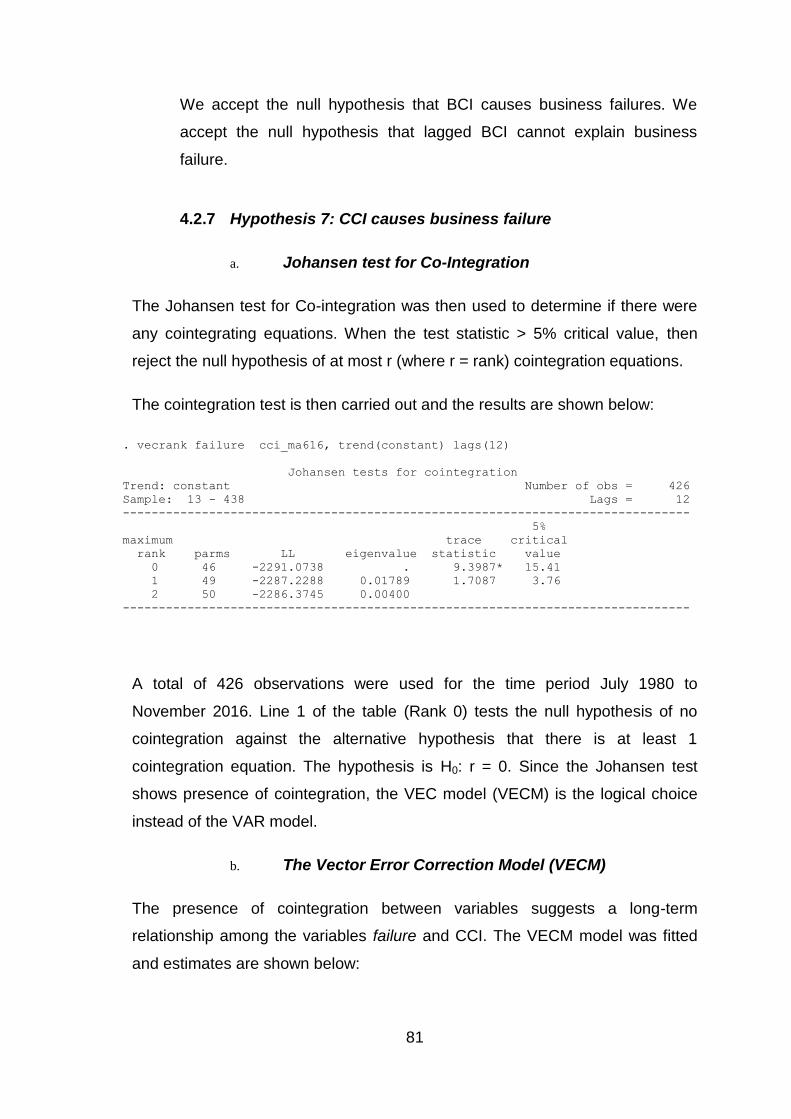
81
We accept the null hypothesis that BCI causes business failures. We
accept the null hypothesis that lagged BCI cannot explain business
failure.
4.2.7 Hypothesis 7: CCI causes business failure
a. Johansen test for Co-Integration
The Johansen test for Co-integration was then used to determine if there were
any cointegrating equations. When the test statistic > 5% critical value, then
reject the null hypothesis of at most r (where r = rank) cointegration equations.
The cointegration test is then carried out and the results are shown below:
. vecrank failure cci_ma616, trend(constant) lags(12)
Johansen tests for cointegration
Trend: constant Number of obs = 426
Sample: 13 - 438 Lags = 12
-------------------------------------------------------------------------------
5%
maximum trace critical
rank parms LL eigenvalue statistic value
0 46 -2291.0738 . 9.3987* 15.41
1 49 -2287.2288 0.01789 1.7087 3.76
2 50 -2286.3745 0.00400
-------------------------------------------------------------------------------
A total of 426 observations were used for the time period July 1980 to
November 2016. Line 1 of the table (Rank 0) tests the null hypothesis of no
cointegration against the alternative hypothesis that there is at least 1
cointegration equation. The hypothesis is H0: r = 0. Since the Johansen test
shows presence of cointegration, the VEC model (VECM) is the logical choice
instead of the VAR model.
b. The Vector Error Correction Model (VECM)
The presence of cointegration between variables suggests a long-term
relationship among the variables failure and CCI. The VECM model was fitted
and estimates are shown below:
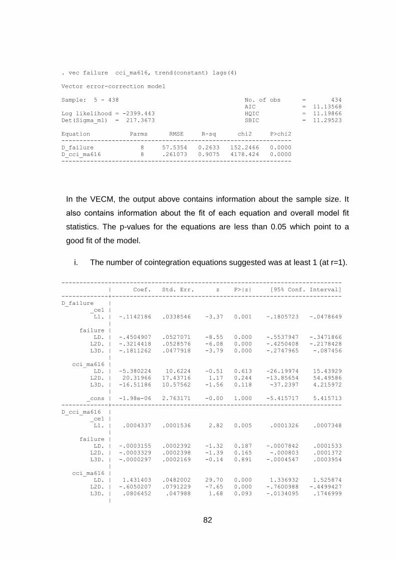
82
. vec failure cci_ma616, trend(constant) lags(4)
Vector error-correction model
Sample: 5 - 438 No. of obs = 434
AIC = 11.13568
Log likelihood = -2399.443 HQIC = 11.19866
Det(Sigma_ml) = 217.3673 SBIC = 11.29523
Equation Parms RMSE R-sq chi2 P>chi2
----------------------------------------------------------------
D_failure 8 57.5354 0.2633 152.2466 0.0000
D_cci_ma616 8 .261073 0.9075 4178.424 0.0000
----------------------------------------------------------------
In the VECM, the output above contains information about the sample size. It
also contains information about the fit of each equation and overall model fit
statistics. The p-values for the equations are less than 0.05 which point to a
good fit of the model.
i. The number of cointegration equations suggested was at least 1 (at r=1).
------------------------------------------------------------------------------
| Coef. Std. Err. z P>|z| [95% Conf. Interval]
-------------+----------------------------------------------------------------
D_failure |
_ce1 |
L1. | -.1142186 .0338546 -3.37 0.001 -.1805723 -.0478649
|
failure |
LD. | -.4504907 .0527071 -8.55 0.000 -.5537947 -.3471866
L2D. | -.3214418 .0528576 -6.08 0.000 -.4250408 -.2178428
L3D. | -.1811262 .0477918 -3.79 0.000 -.2747965 -.087456
|
cci_ma616 |
LD. | -5.380224 10.6224 -0.51 0.613 -26.19974 15.43929
L2D. | 20.31966 17.43716 1.17 0.244 -13.85654 54.49586
L3D. | -16.51186 10.57562 -1.56 0.118 -37.2397 4.215972
|
_cons | -1.98e-06 2.763171 -0.00 1.000 -5.415717 5.415713
-------------+----------------------------------------------------------------
D_cci_ma616 |
_ce1 |
L1. | .0004337 .0001536 2.82 0.005 .0001326 .0007348
|
failure |
LD. | -.0003155 .0002392 -1.32 0.187 -.0007842 .0001533
L2D. | -.0003329 .0002398 -1.39 0.165 -.000803 .0001372
L3D. | -.0000297 .0002169 -0.14 0.891 -.0004547 .0003954
|
cci_ma616 |
LD. | 1.431403 .0482002 29.70 0.000 1.336932 1.525874
L2D. | -.6050207 .0791229 -7.65 0.000 -.7600988 -.4499427
L3D. | .0806452 .047988 1.68 0.093 -.0134095 .1746999
|
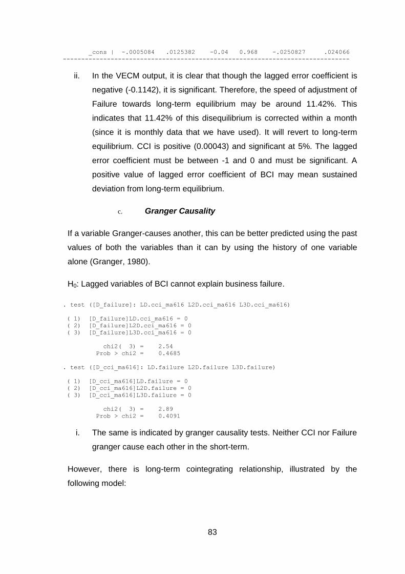
83
_cons | -.0005084 .0125382 -0.04 0.968 -.0250827 .024066
------------------------------------------------------------------------------
ii. In the VECM output, it is clear that though the lagged error coefficient is
negative (-0.1142), it is significant. Therefore, the speed of adjustment of
Failure towards long-term equilibrium may be around 11.42%. This
indicates that 11.42% of this disequilibrium is corrected within a month
(since it is monthly data that we have used). It will revert to long-term
equilibrium. CCI is positive (0.00043) and significant at 5%. The lagged
error coefficient must be between -1 and 0 and must be significant. A
positive value of lagged error coefficient of BCI may mean sustained
deviation from long-term equilibrium.
c. Granger Causality
If a variable Granger-causes another, this can be better predicted using the past
values of both the variables than it can by using the history of one variable
alone (Granger, 1980).
H0: Lagged variables of BCI cannot explain business failure.
. test ([D_failure]: LD.cci_ma616 L2D.cci_ma616 L3D.cci_ma616)
( 1) [D_failure]LD.cci_ma616 = 0
( 2) [D_failure]L2D.cci_ma616 = 0
( 3) [D_failure]L3D.cci_ma616 = 0
chi2( 3) = 2.54
Prob > chi2 = 0.4685
. test ([D_cci_ma616]: LD.failure L2D.failure L3D.failure)
( 1) [D_cci_ma616]LD.failure = 0
( 2) [D_cci_ma616]L2D.failure = 0
( 3) [D_cci_ma616]L3D.failure = 0
chi2( 3) = 2.89
Prob > chi2 = 0.4091
i. The same is indicated by granger causality tests. Neither CCI nor Failure
granger cause each other in the short-term.
However, there is long-term cointegrating relationship, illustrated by the
following model:
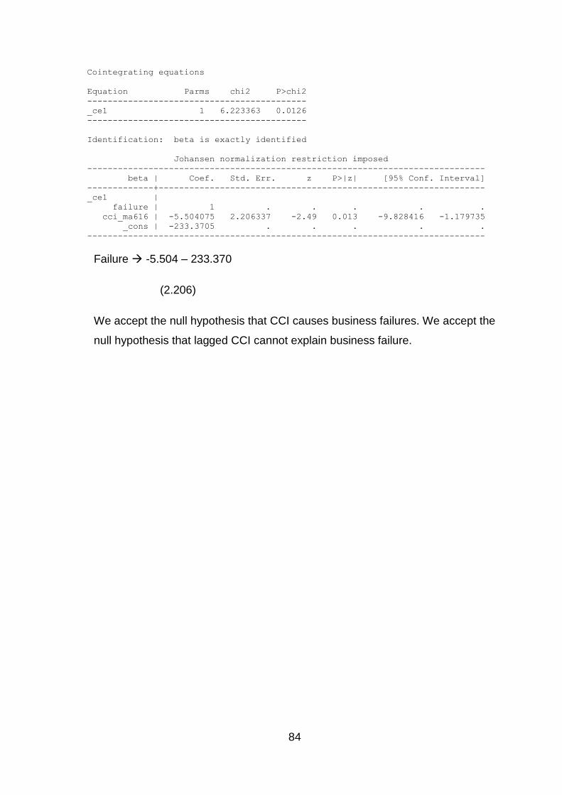
84
Cointegrating equations
Equation Parms chi2 P>chi2
-------------------------------------------
_ce1 1 6.223363 0.0126
-------------------------------------------
Identification: beta is exactly identified
Johansen normalization restriction imposed
------------------------------------------------------------------------------
beta | Coef. Std. Err. z P>|z| [95% Conf. Interval]
-------------+----------------------------------------------------------------
_ce1 |
failure | 1 . . . . .
cci_ma616 | -5.504075 2.206337 -2.49 0.013 -9.828416 -1.179735
_cons | -233.3705 . . . . .
------------------------------------------------------------------------------
Failure -5.504 – 233.370
(2.206)
We accept the null hypothesis that CCI causes business failures. We accept the
null hypothesis that lagged CCI cannot explain business failure.
85
5 CHAPTER 5: DISCUSSION OF THE RESULTS
5.1 Introduction
This chapter will seek to relate and compare the results presented and analysed
in Chapter 4 pertaining to the hypotheses, and link the findings to the relevant
academic literature presented in Chapter 2. Findings are compared and
analysed by individual hypotheses and research questions. After ascertaining if
there is a relationship between these findings and those of other academics,
this research is concluded, having noted any discrepancies and relationships
that are of significance. Therefore, the chapter addresses the following areas:
explaining the models used in this study, their limitations, and the data results,
and lastly how the different hypotheses are addressed. The data analysis for
this study was conducted using STATA Version 12.
The study has empirically examined the business failure of companies in South
Africa by modelling business failure and macroeconomic variables.
Macroeconomic variables in the study include GDP and CPI. The CPI is
modelled as a proxy to inflation. The other macroeconomic variables include
those of recent and past business cycle, which are the composite leading
(CBCL), composite coincident (CBCC), and composite lagging (CBCG)
indicators. Additionally, there are variables of business confidence index (BCI)
and consumer confidence index (CCI), which are more behaviour-based. The
study uses both consumption-based variables to understand the aspect of
purchasing power indirectly, and some behaviour-based variables to
understand what motivates buying. Moreover, Composite Business Cycles were
used to understand if macro factors based on their cycle of lead, coincident, and
lag influence business failure. However, it is more likely that the generic macro
factors are not sufficient in explaining failure over time. The study, therefore,
added behavioural confidence indices in the model in the form of Business and
Consumer Confidence Indices.
The majority of research that was conducted on business failure emphasised
the one-way causality from macroeconomic variables to aggregate business
86
failure. While the case for reverse causality from business failure has been
tested in the process, it has not been the focus of the study. One can point out
that business failure can also be modelled as an independent variable, and it
can be constituted as a causal factor for fluctuations or changes or volatility of
macroeconomic factors, but that is beyond the scope of this study.
The rest of the study is organized as such: models used in the study are
discussed, also giving the econometric details of each model; the results
obtained for the tests that are derived from the models; a summary of findings;
and a conclusion.
5.2 Models used in the study
Models used were based on the nature of the data. The study uses secondary
data for the analysis. Though the credibility of the source of data can be
established, the data being economic in nature cannot be undermined.
Different models were employed to allow for systemic analysis of the data into
information that can be interpreted easily and hence help in testing the set
hypotheses.
5.2.1 Augmented Dickey Fuller Test
The first step in analysis was to understand the stationarity of the series under
consideration. Since the study uses economic data, issues like non-stationarity
and autocorrelation are commonplace. So, the first test was a stationarity test.
The most commonly employed test is the Augmented Dickey-Fuller test (ADF)
(Dickey & Fuller, 1979). This is the unit root test for stationarity. Unit roots can
cause spurious results in the time series analysis. Non-stationarity and data
instability may have severe repercussions for the traditional failure of prediction
models that can lead to poor predictive abilities in future dated samples
(Mensah, 1984). The model used in the study is an augmented version of the
Dicker fuller test and can handle larger and more complex sets of time series
87
models than the prior version. The ADF model is nothing but a regression
model, which is as follows:
∆yt = α + βyt−1 + δt + X k j=1 ζj∆yt−j + et
where y is the dependent variable, α is the constant, β is the coefficient, δt is
the time trend, k is the number of lags in the model, and e is the error term or
disturbance. The null hypothesis for the ADF test is:
H0 : The series contain a unit root (or in other words, the series is a random
walk).
The ADF statistic used in the test is a negative number in which the stronger the
negative, the stronger the rejection of the hypothesis that there is a unit root at
some level of confidence. Considering that the data being investigated by this
study is time dependent, the choice of this method of testing was made with the
aim of testing the null hypothesis of a Unit root in the time series of information
on business failures in South Africa.
It is important to inspect the available data before running an ADF test so as to
figure out an appropriate regression model. For example, a non-zero mean
indicates the regression will have a constant term. After the selection of a
regression model, it is important to then use the ADF to add lagged differences
to these models.
In the analysis in the previous chapter the Augmented Dickey-Fuller test was
conducted to ascertain if the series were non-stationary. In each case, for each
series, the p-value was observed. If the p-value was below 0.05 (at 95%
significance), then the null hypothesis was rejected, and it was concluded that
the series was stationary. This method’s major limitation is that there is a size
distortion for most tests, so the null distribution is available only asymptotically.
Moreover, it is often argued that the finite sample distribution is differs
substantially from the asymptotic one, leading to actual rejection rates that differ
substantially from the nominal level. Classic statistical failure prediction models
assume that the relationship between the independent and dependant variables
are stable over time and remain the same through the panel time-series data
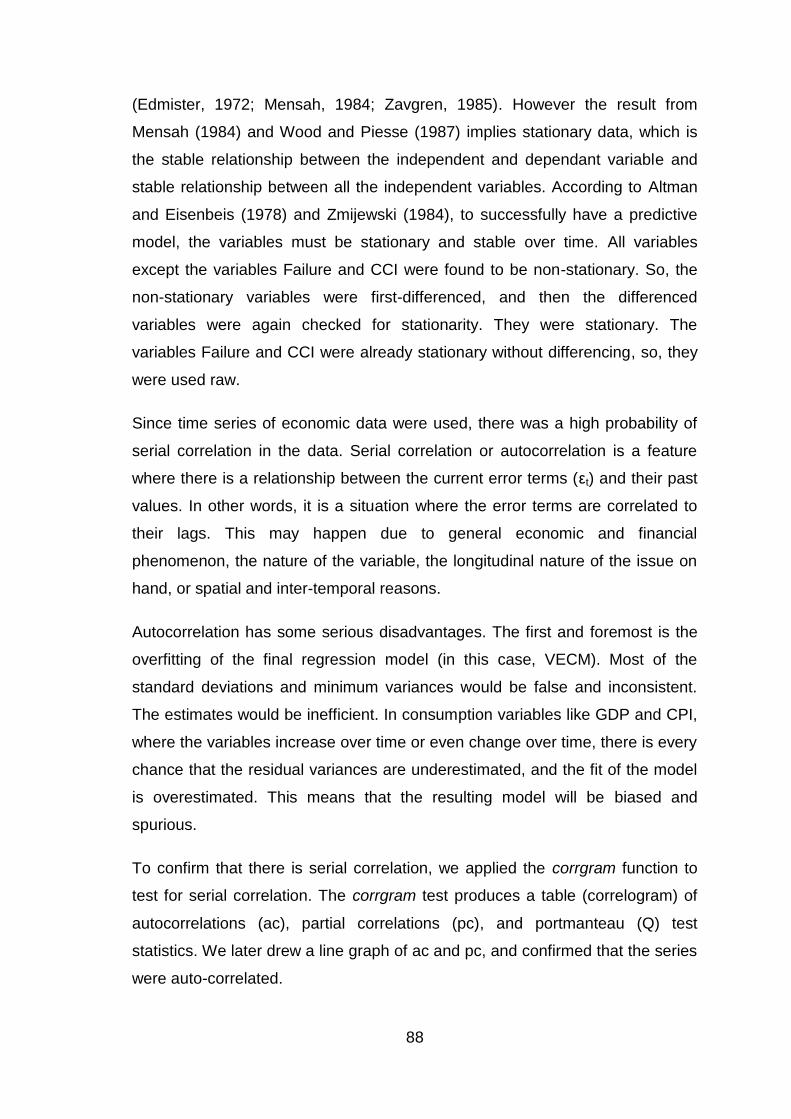
88
(Edmister, 1972; Mensah, 1984; Zavgren, 1985). However the result from
Mensah (1984) and Wood and Piesse (1987) implies stationary data, which is
the stable relationship between the independent and dependant variable and
stable relationship between all the independent variables. According to Altman
and Eisenbeis (1978) and Zmijewski (1984), to successfully have a predictive
model, the variables must be stationary and stable over time. All variables
except the variables Failure and CCI were found to be non-stationary. So, the
non-stationary variables were first-differenced, and then the differenced
variables were again checked for stationarity. They were stationary. The
variables Failure and CCI were already stationary without differencing, so, they
were used raw.
Since time series of economic data were used, there was a high probability of
serial correlation in the data. Serial correlation or autocorrelation is a feature
where there is a relationship between the current error terms (εt) and their past
values. In other words, it is a situation where the error terms are correlated to
their lags. This may happen due to general economic and financial
phenomenon, the nature of the variable, the longitudinal nature of the issue on
hand, or spatial and inter-temporal reasons.
Autocorrelation has some serious disadvantages. The first and foremost is the
overfitting of the final regression model (in this case, VECM). Most of the
standard deviations and minimum variances would be false and inconsistent.
The estimates would be inefficient. In consumption variables like GDP and CPI,
where the variables increase over time or even change over time, there is every
chance that the residual variances are underestimated, and the fit of the model
is overestimated. This means that the resulting model will be biased and
spurious.
To confirm that there is serial correlation, we applied the corrgram function to
test for serial correlation. The corrgram test produces a table (correlogram) of
autocorrelations (ac), partial correlations (pc), and portmanteau (Q) test
statistics. We later drew a line graph of ac and pc, and confirmed that the series
were auto-correlated.
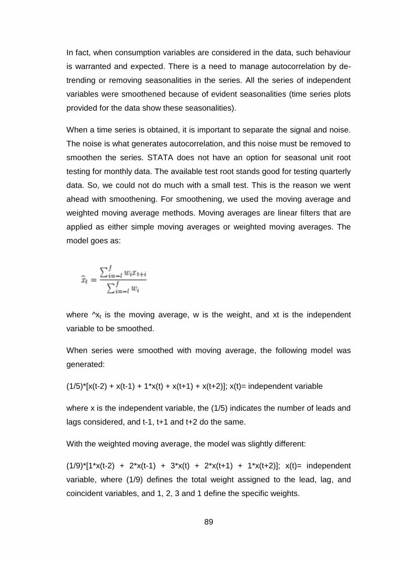
89
In fact, when consumption variables are considered in the data, such behaviour
is warranted and expected. There is a need to manage autocorrelation by de-
trending or removing seasonalities in the series. All the series of independent
variables were smoothened because of evident seasonalities (time series plots
provided for the data show these seasonalities).
When a time series is obtained, it is important to separate the signal and noise.
The noise is what generates autocorrelation, and this noise must be removed to
smoothen the series. STATA does not have an option for seasonal unit root
testing for monthly data. The available test root stands good for testing quarterly
data. So, we could not do much with a small test. This is the reason we went
ahead with smoothening. For smoothening, we used the moving average and
weighted moving average methods. Moving averages are linear filters that are
applied as either simple moving averages or weighted moving averages. The
model goes as:
where ^xt is the moving average, w is the weight, and xt is the independent
variable to be smoothed.
When series were smoothed with moving average, the following model was
generated:
(1/5)*[x(t-2) + x(t-1) + 1*x(t) + x(t+1) + x(t+2)]; x(t)= independent variable
where x is the independent variable, the (1/5) indicates the number of leads and
lags considered, and t-1, t+1 and t+2 do the same.
With the weighted moving average, the model was slightly different:
(1/9)*[1*x(t-2) + 2*x(t-1) + 3*x(t) + 2*x(t+1) + 1*x(t+2)]; x(t)= independent
variable, where (1/9) defines the total weight assigned to the lead, lag, and
coincident variables, and 1, 2, 3 and 1 define the specific weights.
90
Creating these filters was dependent on the noise reducing phenomenon. Each
time a moving or weight moving average was applied, the line graph for the
noise was checked. Both moving averages and weighted moving averages
were applied to the series until the noise was reduced sufficiently and the
autocorrelation was removed to the largest extent possible. Smoothening was
applied to all independent variable series, and thereafter, the smoothed series
were used for further analysis.
5.2.2 The Johansen test for co-integration
We have already seen that the series are first difference stationary, in other
words, integrated to the order 1 or I (1). It is not a covariance stationary process
or an I (0).
Cointegration is again a feature that is unique to time series, especially
economic and financial data. Cointegration is defined as the movement of two
time series together, over time in simple terms (Johansen, 1988). So, two
independent variables or the dependent and independent variables are said to
be cointegrated when there is a parameter a, which forms a relationship like:
ut = DVt − aIVt
So, if xt1 and xt2 are two independent variables that are I(1) and both have
random walk, then a linear combination of them will also have a random walk
and a common stochastic trend. This is cointegration, and the variables are
cointegrated with a cointegrating vector β.
While such a relationship is expected of economic and financial series, and
especially of time series, it is important to know this relationship and incorporate
this in the final model so that the regression is complete with short-term and
long-term relationships between the variables.
The Johansen test for Co-Integration was conducted to assess if there was a
long-term cointegrating relationship between failure and each of the
independent variables (Johansen, 1988).
91
If the test statistic is less than the critical value, you reject the null hypothesis of
at most the rank co-integration equations. The number of lags was selected via
the varsoc (pre-estimation test) in STATA. We chose 12 lags for the lag
determination exercise, giving importance to the nature of the data that we
selected (monthly data). As a result, the number of lags determined for each
variable was 10, 11 or 12. For Failure, the number of lags determined was 5.
The cointegration test was done for each variable, and the test indicated at least
one cointegration model that would be present.
5.2.3 The Vector Error Correction Model (VCEM)
To sustain equilibrium, there must be forces that pull the cointegrated variables
towards equilibrium. So, if two independent variables or an independent and
dependent variable are cointegrated, an error correction model must be present
to pull them towards equilibrium. The Vector Error Correction Model is just that.
The VECM’s clarity is in its values of error coefficients. For the disequilibrium to
be filled up, at least one lagged error coefficient needs to be negative (and
significant at 5%); for one independent variable we need α1 to be negative, and
the other needs to be positive.
The VECM model is an adjusted model of the vector autoregressive model to
take into accounts the co-integrating relationships and non-stationarity among
the variables.
The Vector Error Correction Model was fitted to assess whether there was a
long-term relationship between failure and each of the other variables (CPI).
The presence of co-integration between variables would have suggested a
long-term relationship between the variables exists. The VECM assesses the
relationship but does not assess the direction in terms of the flow of the
relationship. The vector correction model states that the total change in y can
be decomposed in response a response to the last period’s disequilibrium, a
moving average of past changes, and white noise (Liu, 2009).
92
In our study, we found that CPI and business failure are not related in the long-
term, which is the case with CBCC, CBCL, and GDP. But in the case of CBCG,
it was found that the error coefficient was positive (0.004087) and insignificant.
Therefore, the speed of adjustment of Failure towards long-term equilibrium
cannot be concluded clearly. However, CBCG was negative (-0.0001306),
which is a value very near to 0 and is significant at 5%. This indicates that 0.013
percent of this disequilibrium is corrected within a month (since it is monthly
data that we used). It will revert to long-term equilibrium. It may be concluded
that Failure causes CBCG. CBCG is the composite lagging business cycle.
When there are business failures, the composite lagging business cycle
changes in the short-term. The long-term relationship is illustrated by the
cointegrating relationship. BCI and CCI are also explained by the VECM. In the
VECM output, it is clear that though the error coefficient is negative (-0.1266), it
is significant. Therefore, the speed of adjustment of Failure towards long-term
equilibrium may be around 12%. This indicates that 12% of this disequilibrium is
corrected within a month (since it is monthly data that we have used). It will
revert to long run equilibrium. Similarly, in case of CCI, the speed of adjustment
of Failure towards long-term equilibrium may be around 11.42%. This indicates
that 11.42% of this disequilibrium is corrected within a month (since it is monthly
data that we have used). It will revert to long-term equilibrium.
5.2.4 Granger Causality
Granger causality is a model that predicts if past values of the first variable are
useful in predicting past values of the second variable. In other words, granger
causality assesses the direction of the relationship, which cannot be determined
by the VCEM. It is a statistical hypothesis of determining whether one-time
series is useful in forecasting another. If a variable Granger-causes another,
this can be better predicted using the past values of both the variables than it
can by using the history of one variable alone (Granger, 1980). Granger
causality is employed to establish whether or not the macroeconomic variables
investigated in this study can be utilized to predict the probability of business
failures. In this case, it evaluates the effect of one on the other and vice versa.
93
It was found that business failures can granger-cause CBCL.
5.3 Summary of findings
This hypothesis that CPI causes business failures is not supported, and it is
concluded that the number of business failures do not respond to disequilibrium
between consumer price index and failure. In the same way, CPI also does not
respond to disequilibrium between consumer price index and failure. This
means that changes in the CPI do not affect the business failure in the case of
South Africa. This is in contrast to the study by Everett and Watson (1998) who
found that a declining consumer price index leads to business failure due to a
fall in purchasing power of the consumer. In the long run, there is no causality
between CPI and the number of business failures. This can also mean that in
South Africa inflation and fluctuations of the CPI do not make a difference to
number of business failures.
The hypothesis that GDP causes business failure rates is not supported, and it
is concluded that GDP does not cause business failure and business failures do
not contribute to GDP changes. The gross domestic product, therefore, is not
directly related to the number of business failures in South Africa, which
translates to too few failed businesses. It is agreed that liquidity constraints in
each country are an essential macroeconomic factor determined by the GDP
growths, which bears significant influence on business success. This can in fact
be proven; greater asset base is often associated with increased rates of
business entry during times of economic growth (Fairlie & Krashinsky, 2012).
Also, this is supported by research by Liu (2009) who noted that sudden
declines in the economic performance at the international or national levels bear
significant impacts on the performance of businesses. However, GDP seems a
far-fetched case in this study, as businesses (and consequently, the number of
business failures) seem a microeconomic variable in terms of relating them to
GDP. GDP is a macroeconomic consumption variable, which accounting for not
just business consumption, but also household consumption, including imports,
exports, and much more. So, business failures may be too small to actually
affect GDP, at least directly.
94
The hypothesis that CBCL causes business failures is not supported, and it is
concluded that CBCL does not affect business failure and the number of
business failures also do not affect CBCL. However, there was short-term
causality running from failure of businesses to CBCL, indicating that the
composite leading business cycle indicator may be useful in predicting business
failures. This is logical because business cycles and their trends are used by
businesses to understand future prices and economics, and therefore, it is
possible that business failures can be predicted by composite lead indicators of
business cycles.
The hypothesis that CBCC causes business failures is not supported, and it is
concluded that CBCC does not affect business failure. Conversely, number of
business failures does not affect CBCC. There is no long-term relationship
between the variables.
The hypothesis that CBCG causes business failures is supported. Business
failure causes the composite lagging business cycle indicator to change. Labour
cost per unit of production, ratio of inventories to sales in the manufacturing and
trade sectors, other operational variables, and predominant prime overdraft rate
of banks and other similar components form the lagging business indicators
(Van der Walt, 1983; Van der Walt & Pretorius, 1994; Venter & Pretorius, 2004;
Venter, 2004). Past values of these variables logically affect current time
period’s business performance. This is indicated well by the VECM result.
Whenever there is a shortage of labour, high unemployment, saturation in the
labour market, or low supply of labour, the cost of labour in businesses is
affected, which would in turn affect the performance of the business. Moreover,
since there are other operational variables also in the lagging indicator, this
affects businesses. This, in the long term, may lead to exit or failure. The time
period (∆) considered for the study is a month. In this sense, the previous
month’s labour market variables would most likely affect the current month’s
business performance.
The hypothesis that BCI causes business failures is supported, and it is
concluded that an increase in BCI leads to a decrease in business failures. In
95
addition, that business failure also affects BCI and the previous values of
business failures affect BCI. For example, in South Africa business recession is
characterized by poor performance in annual turnover and consumer appeal to
its products. These factors impact on the quality of the businesses, such as
deteriorating financial stabilities (De Loecker & Van Biesebroeck, 2016). As can
be noted declining business failure rates are characterized by low production
levels, few or no orders, and low stock levels, which are the main variables for
computation of the business confidence index. They also relate to the labour
productivity in manufacturing of business personnel in the company. This
justifies the findings of Honjo (2000), who concluded that a close relationship
between the returns accrued from the business and the risks of its consequent
operations exists.
The hypothesis that CCI causes business failures is supported, and it is
concluded that CCI affects business failure though the number of business
failures do not affect CCI. This is because consumers tend to decrease erratic
spending in high inflationary cycles, which directly influences profitability of the
business. Consumers are the sole revenue generating source for businesses,
so if they cut their spending it leads to business failures. Consumer confidence
is influenced by the individual consumer’s perception of the economy on the
expected future patterns of growth or recession, which directly impacts savings
and spending. It is measured by the consumer purchasing trends mostly on
high-end items compared to basic necessities.
5.4 Conclusion
Past research on the relationship between macroeconomic aggregates and
business failures have been limited to the short-term relationships between the
variables. Research analysis on this study has used an error-correction model
(VECM) to explore the causes of South African business failures by modelling
the short- and long-term behaviours of business failure rates in relation to
macroeconomic business cycles over the period 1980-2016.
96
The objective of this study was to analyse the relationship between business
failure and fluctuations associated with the macroeconomic business cycles
focusing on South African businesses over a 36-year period. Based on the
analysis, the association between business cycles and the macroeconomic
influences has been significant to the business failures and fluctuations. This
empirical study indicates that there exists a normal, dynamic relationship
between macro economy and corporate failure rates.
The VECM analysis confirms the positive impact the Macroeconomic variables
have on business failure rates. Though it is not indicated in this study, there is
an econometric, as well as economic impact, of inflation on business failures.
This has in fact been indirectly shown via the relationship of business
confidence and consumer confidence indices with business failures. Therefore,
it is safe to reiterate that high rates of inflation may indicate long-term issues
within the country’s economy, as well as salaries being linked to inflation
potentially hurting the business bottom line (Everett & Watson, 1998).
Wadhwani (1986) argued that in the absences of index-linked loans, increased
inflation implies higher liquidation rates, and Millington (1994) reported inflation
as a significant correlation to business failure rates.
Results in the research by Liu (2009) indicate that the long-run and short-run
effects of inflation shock indicate that high inflation rates lead to a rise in
business failure rates. According to Liu (2009), this finding lends credibility to
the argument that high inflation rates can be costly to the economy.
Furthermore, the positive shock to inflation generates an initial short-lived fall in
business failures followed by a long-term rise in both periods. Its adverse effect
ultimately falls on the rate of business failures, and the effect is shown to be five
times stronger in the pre-1980 period to reflect the influence of the inflationary
economy in the period. The findings from the two periods lend support to the
claim of Wadhwani (1986) that inflation raises the bankruptcy rate for
businesses. The pattern of the responses of business failure rates to the
business birth rate shock appears to be similar in both periods, with the stronger
effect seen in the pre-1980 period. We observe the significant but opposite role
97
of business incorporations in business failures over time. In the short-run, an
increase in new company incorporations results in a decrease in failure rates
within the first few periods of establishment, confirming the ‘honeymoon’ effect
reported by Altman (1983) and Hudson (1986). However, in the medium to long-
run, they are positively correlated.
According to Santoro and Gaffeo (2009), they have established that the
bankruptcy rate closely moves together with macroeconomic variables and that
the identification of the long-run proportional relationship has effects for
academics and corporate businesses by informing institutions of credit risk
management. Santoro and Gaffeo (2009) have identified the causal running
from macroeconomic variables to bankruptcies but have not found this to hold
true the other way around. Additionally, Santoro and Gaffeo (2009) have
established short-term aggregate shocks on the bankruptcy rate to be the same
as long-term.
Business confidence plays a significant role in understanding behavioural
aspects of business owners as well as consumers. The BCI developed in South
Africa is the indicator for prevailing business and economic conditions. This
affects business failures and exits because businesses form important parts of
value chains in an economic environment, small or large. This is directly related
to the consumer confidence index (CCI) because consumers form the other end
of the chain. The burden of prices or the rewards of discounts are passed on to
consumers whose purchasing power matters the most. Business operations,
maintenance, and failures are all dependent on consumers and their confidence
because businesses produce for consumers. In fact, the types of consumers
may be more in number than the types of business owners, because most
business owners are also consumers. This means that CCI affecting business
failures is quite a logical relationship found by the model in this study.
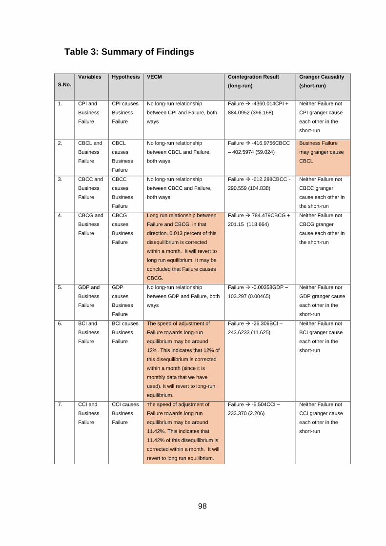
98
Table 3: Summary of Findings
S.No.
Variables Hypothesis VECM Cointegration Result
(long-run)
Granger Causality
(short-run)
1. CPI and
Business
Failure
CPI causes
Business
Failure
No long-run relationship
between CPI and Failure, both
ways
Failure -4360.014CPI +
884.0952 (396.168)
Neither Failure not
CPI granger cause
each other in the
short-run
2, CBCL and
Business
Failure
CBCL
causes
Business
Failure
No long-run relationship
between CBCL and Failure,
both ways
Failure -416.9756CBCC
– 402.5974 (59.024)
Business Failure
may granger cause
CBCL
3. CBCC and
Business
Failure
CBCC
causes
Business
Failure
No long-run relationship
between CBCC and Failure,
both ways
Failure -612.288CBCC -
290.559 (104.838)
Neither Failure not
CBCC granger
cause each other in
the short-run
4. CBCG and
Business
Failure
CBCG
causes
Business
Failure
Long run relationship between
Failure and CBCG, in that
direction. 0.013 percent of this
disequilibrium is corrected
within a month. It will revert to
long run equilibrium. It may be
concluded that Failure causes
CBCG.
Failure 784.479CBCG +
201.15 (118.664)
Neither Failure not
CBCG granger
cause each other in
the short-run
5. GDP and
Business
Failure
GDP
causes
Business
Failure
No long-run relationship
between GDP and Failure, both
ways
Failure -0.00358GDP –
103.297 (0.00465)
Neither Failure nor
GDP granger cause
each other in the
short-run
6. BCI and
Business
Failure
BCI causes
Business
Failure
The speed of adjustment of
Failure towards long-run
equilibrium may be around
12%. This indicates that 12% of
this disequilibrium is corrected
within a month (since it is
monthly data that we have
used). It will revert to long-run
equilibrium.
Failure -26.306BCI –
243.6233 (11.625)
Neither Failure not
BCI granger cause
each other in the
short-run
7. CCI and
Business
Failure
CCI causes
Business
Failure
The speed of adjustment of
Failure towards long run
equilibrium may be around
11.42%. This indicates that
11.42% of this disequilibrium is
corrected within a month. It will
revert to long run equilibrium.
Failure -5.504CCI –
233.370 (2.206)
Neither Failure not
CCI granger cause
each other in the
short-run
99
6 CHAPTER 6: CONCLUSIONS OF THE STUDY
6.1 Introduction
The study sought to understand business failure due to changing business
cycles using set indicators relevant to South Africa. In this chapter conclusions
of the study are presented, followed by implications, recommendations, and
suggestions for future research.
6.2 Conclusions of the study
The research study makes a significant contribution towards academic literature
by indicating the importance of systemic and un-systemic risk that relates to
business failure. The importance of business failure risk, governmental policies,
such as monetary and financial ones that must be adopted to reduce risk of
business failure, and the policies that individual businesses must adopt, are
detailed.
The study has adopted quantitative research techniques to analyse time series
economic data. This has provided interesting results that are in agreement with
both theory and practical applications. It is understood that the influence of
macroeconomic factors on the business cycles around the world cannot be
underestimated. Business cycles, per se, are key components of understanding
and forecasting business performance, failure and exit. Economic expansions
and contractions are categorised as leading, lagging, and composite variables
in the study, to take into account different stages of the business cycle and to
understand different variables that influence business failures at different points
in the cycle.
Economic cycles in their decline phase also affect business profitability Geroski
and Machin (1993) and have a direct impact on a company’s sustainability
reducing revenue, thereby influencing business failures (Everett & Watson,
1998). It is important to note that a business cycle comprises various
expansions occurring at almost the same time, this affects various economic
100
activities followed by a similar recession, contraction, and revivals in economic
performance which merge up into the next expansion phase. In his research,
Liu (2009) found that in the medium to long-term, business failures increase as
a consequence of a rise in new business incorporations within the economy.
This results from the entry of multi-national corporations attracted by a growing
GDP, leading to the sudden failure of small unstable businesses in the same
field.
Apart from the post-war economists, contemporary economists have utilised
these variables often to describe the economic conditions of different regions
and their consequent influences on business activities.
There are various reasons for business failures in South Africa. The most
common reasons are poor business plans, inflation, bankruptcy, and global
recession. The study adopts an appropriate approach to investigate the effects
of such variables on the dependent variable, which is the number of business
failures. To investigate the effect on failure rates, an error-correction model was
utilized, as it aided the interpretation of the properties of the business failure
model within a framework of the long-term equilibrium, coupled with its short-
term dynamic adjustment process of the economic variables.
The leading business cycle indicators of South Africa are: commodity price
index for South Africa’s main export commodities; business confidence index,
the composite leading business cycle indicator for South Africa’s major trading-
partner countries; number of building plans approved; interest rate spread, real
m1; and more. The business confidence index is a significant indicator for the
business cycle in evaluating and determining the macroeconomic fluctuations,
and this was weak. Reports such as those by Bishop (2016) indicated that
business owners were dissatisfied with the business climate in South Africa,
and therefore, a weak growth was expected in 2016. However, in general, there
were no predictions of business failures or exits.
Lagging business indicators in South Africa include: employment and labour
components like employment and unemployment in agriculture; the number of
101
appointments per 100 production workers; consumption and trade orders;
labour costs in production; and other allied variables (Van der Walt, 1983; Van
der Walt & Pretorius, 1994; Venter, 2004). All these are operational variables
which affect business performance directly. So, it is logical that lagging
composite business cycle indicators showed a relationship with business
failures.
Coincident business cycle indicators did not show any relationship, reiterating
the fact that businesses are affected more by past values of factors and
variables rather than current values of factors and variables.
It was observed that business confidence index and consumer confidence index
had individual relationships with business failures. Both these indices predict
the business environment in the economy and drive sales, production and
employment. These three variables form the pillars of an economy, especially
household consumption and industrial consumption, which are driven by the
confidence indices. The analysis in this study showed appropriate and
respective relationships.
6.3 Implications and recommendations
In order to understand the impact of business failures on the economy, it is also
important to describe how businesses are impacted by the various indicators in
the economy and how to counter them. Falling consumer confidence means
that there is low spending within the economy, which may mean that
businesses must adjust their production schedules significantly. This requires
lowering the output and creating a scarcity within the economy to enhance
demand. Such production cuts mean that it is easy to reduce overhead costs in
relation to sales achieved, which enhance profitability of a business during hard
economic times.
Government regulations to appropriate low purchasing power of the consumers
are directly related to the ease of capital borrowing and interest rates on loans
borrowed. This relates to corrective policies on interest and inflation, which
102
affect consumer access to capital. Findings from the research on this paper go
beyond business failures. The monetary policy department from the South
African regulatory departments can apply the results within their policies to
potentially stabilise the economy through informed cause and affect changes in
the macro environment. Understanding why and how businesses fail and what
impacts these failures, and in turn how these impact the economy, can generate
policies that can mitigate risk, especially business failure risk. Response
measures can also be found.
Growth in unemployment rates is directly related to the rate of business failures.
As a result, a receding GDP means less output, and as a circular effect,
employment rates fall short of what is needed for economic stability. In South
Africa, confidence levels at the household/consumer level have been declining;
a key concern has been persistently high levels of unemployment faced within
the economy with a subdued income growth in developing countries. For
businesses, sluggish demand and highly competitive operating conditions
continue to influence perception of resilience and confidence. It is appropriate
for a country like South Africa to put in place policies that bolster or spur
economic growth to boost the aggregate GDP, leading to more business start-
ups creating a large employment base. This can be implemented by using both
the supply side and demand side policies.
There are some socioeconomic concerns that need addressed, which would
impact businesses and the GDP alike, even if such an effect would be seen
rather gradually. In South Africa, there are many individuals who have
inadequate education and financial training on monetary policies. This means
that there is insufficient business knowledge among entrepreneurs, increasing
the likelihood of business failure. There is lack of economic information that can
aid entrepreneurs to be speculative to determine risk levels for their business
and to develop adequate preventative mechanisms. It is important to prepare
for business upturn cycles and have a good response time to ensure there is no
serious business lag during the cycle period. This observation resonates with
Dubrovski (2009) who maintained that in the event of a crisis within the
business, a quick response is often necessary. It is suggested that the inclusion

103
of entrepreneurship into the school curriculum will nurture and equip learners
with key skills relevant to running a business.
Another major implication is that South Africa’s growth path is highly resource
intensive and thus, unsustainable, which leads to a low business confidence
index. This results from the international market price changes for commodities
such as gold and oil, which creates a major business cycle, upturns if not
correctly predicted. It is highly recommended that risk prediction model is used
to determine the connection between the macroeconomic fluctuations and
business failure since this business failure will impact the economy of South
Africa. There should be corrective measure to ensure that other avenues for
growth are identified and developed. This will create new companies and
eliminate reliance on multinationals that are aligned to natural resources.
For any business to thrive and sustain growth, proper infrastructural provision
should be made available, and for South Africa this has not been achieved.
When this is viewed as a determinant of economic growth there are
inadequacies that are binding constraints. The provision of necessary
infrastructure by government to allow for businesses to grow also plays a key
role in determining whether a business succeeds or fails.
The business failures in South Africa have a significant relationship with the
macroeconomic variables; therefore, it is important for the country to come up
with policies that will significantly reduce the fluctuations and spur economic
growth in the country. A good understanding of the causes of business failures
in a country is the first step towards improving its economy. The cliché that a
problem understood is a problem half-solved applies here in that, by
understanding the microeconomic factors that cause business failures, the
State and other players in the economy can concentrate their efforts on spurring
growth and attracting investors.
104
6.4 Suggestions for further research
This study only limits itself to the understanding of the impact macroeconomic
cycles have on failure of businesses in South Africa. Several opportunities for
further research arose during the process of conducting the study. One of them
is coming up with a solution to streamline the macroeconomic factors that lead
to failure of business as a way of allowing for economic growth and
development. The study was limited to a few macro-economic factors so there
is a need to expand on this research taking note of all other factors that were
not considered in this study. That is why the research question can be tested
with the same model by using different macroeconomic factors.
6.4.1 On a governmental level
Another area that this study leaves open for further exploration is the impact of
political and social inclusion factors of South Africa that may lead to failed
businesses. Cultural values such as hard work and concentration in certain
industries are factors that impact the success or failure of businesses in an
economy. Therefore, it is important to examine these factors to understand their
role in the business world.
Policies set by governments are important to the success of business or the
failure of an economy. Detracting governmental decisions such as increase in
cost of licensing, government control, and political instabilities may also affect
the levels of success for businesses. The provision of necessary infrastructure
to allow for businesses to grow also plays a key role in determining whether a
business succeeds or fails.
6.4.2 On a macro level
It is also important to test the analysed variables further about their relationship
with each other, as it was found during the study’s analysis that some may have
a relationship or impact with/on the other. For example, the composite index of
lagging indicators is best used in conjunction with the composite index of
105
leading indicators to assess their impact on business failure as they tend to be
complimentary in nature. After understanding the macroeconomic fluctuations’
relationship to business failures, the next step would be to address them. This
presents another research opportunity where the different fluctuations can be
examined and solutions sought. With finding solutions to fluctuations that are
not harmful to the businesses in the economy, there is bound to be an
improvement in the levels of business success and the improved economy.
There is need to research the impact of other macro-economic problems like
currency fluctuations, interest rates, and unemployment on the economy at the
various cycle phases. It is important to broaden the area of study as the study
was done on a single economy, which is influenced by other international
economies. Many developing economies are affected by economic changes
experienced in world leading economies such as the UK and the USA. This
was found by (Liu, 2009).
6.4.3 On the business level
Business failure itself has been defined with an arbitrary approach. In the
majority of definitions, failure is linked to bankruptcy (Charitou, Neophytou, &
Charalambous, 2004; Daubie & Meskens, 2002; Dirickx & Van Landeghem,
1994; Ward & Foster, 1997). In addition to the difficulty of defining of failure,
business failure is largely based on a juridical definition. The downside of this
definition is that it does not always include the financial presentation of the
company. Companies can liquidate the assets to avoid paying debt just by
starting a new company. Modelling business failure in predictions analysis can
also be skewed. Failure does not happen overnight and in general panel data
stipulates the date on which the company was officially liquidated but do not
take in consideration the process of company failure (Hubert Ooghe & De
Prijcker, 2008; Theodossiou, 1993)
When searching for literature regarding business failure there were limited
studies done on the subjects compared to prediction models on business failure
(Pretorius, 2009). Evidently, the process of identifying events of business failure
106
are easier to obtain after businesses have failed, than to understand when and
in what stage of a business failure will possibly occur (Probst & Raisch, 2005).
Understanding and defining business literature has presented a theoretical
challenge. Studies in the past have attempted to define literature according to
their methodological approach, especially in prediction models where
bankruptcy and liquidations were general. Future studies can be conducted on
previous literature to attempt to build theory on classifying business failure by
combining financial, legal and regulatory regulations in general use. The benefit
of the unified business failure term is that it can aid business failure prediction
models to be more specific and comparative
Studies in the past have used model-driven architecture models and have
assumed a dichotomous business failure variable which is classified as failed
and not failed. Positioning of the failed versus non-failed business into
populations by itself can cause arbitrary prediction models. In the majority of
studies, a juridical definition of failure has been used of which most systems
classify as bankruptcy. More attempts to identify different classifications of
business failures have produced a variety of results as with Keasey and Watson
(1991) who used financial distress, Laitinen (1991) who used future events such
as cash insolvency and default, and Ward and Foster (1997) who used loan
defaults. The criterion is chosen arbitrarily by researchers, whether it is judiciary
or based on financial distress. Additionally, choosing the failure rate can be
arbitrarily viewed in failing and non-failing businesses when modelled in
percentage, as the increase in births of new businesses can skew the
dichotomous percentage number. As the failure definition is always applied to a
certain arbitrary time period, the separation of firms into failing and no failing
populations is artificial. The two populations are only mutually exclusive within
the chosen time (Altman & Eisenbeis, 1978; H Ooghe & Joos, 1990; H Ooghe
& Verbaere, 1985). Further research can be conducted into defining a unified
methodology when testing for business failure.
According to Bhattacharjee et al. (2009), business failures tend to be cyclical in
nature, where bankruptcies are associated with economic downturn and
107
acquisitions with recoveries. Business failures tend to decline with as
businesses age, and that can contribute to the experience of the firm through
cycles. Additional research can be conducted by introducing the business age,
potentially using the age as a moderating variable.
Additionally, further studies can be made by segmenting the different business
sizes. Everett and Watson (1998) study suggests that economic factors appear
to be associated with 30% to 50% of small business failures, depending on the
definition of failure used.
Balcaen and Ooghe (2006) have argued that although failure should depend on
more than one annual account in financial health, past information about
business performances has been ignored (Pompe & Bilderbeek, 2005;
Shumway, 2001). Further studies can be conducted on company level data of
failed businesses to assess the profitability through business cycles and how
exogenous macro variables influence the business profitability.
However, when panel data is considered, it is usually an indication of a moment
in time, and depending on the definition of business failure, such data can also
be considered. This would lean towards the classic failure prediction models
and would not take into consideration the process of business failure. Detailed
studies can be conducted taking into account the business failure process as
indicated by Ambler et al. (2004) mentioned in the literature review. Moreover,
according to Pretorius (2009), based on literature it is evident that we can learn
from the decline in business, the reasons why businesses fail, and how
business entrepreneurs can make a turnaround to derive more value. Based on
the numerous studies conducted on business failure and the exogenous and
endogenous factors contributing towards business decline and failure, the study
suggests focusing on businesses that were in decline but were eventually able
to turn the businesses into successful entities. Future studies can identify, using
Pretorius (2009) process of business failures, in what stage of the process the
business was in when the turnaround happened. The potential outcomes of the
study can enlighten entrepreneurs and business owners to act proactively
108
based on the findings and to potentially identify a percentage tipping point
where the businesses lost control making failure inevitable.
In conjunction with the above suggestion of understanding the process of
business failure, the classical business failure prediction models do not
differentiate in the possibility that there are different paths for business failure
and assume a uniform process (Laitinen, 1991). Further studies can be
conducted not only in the process of the business failure but can also include
the different paths that lead to failure.
6.4.4 At an industry level
He and Kamath (2006) have indicated that data is generally collected across
industries as a whole and that when the researcher develops a model it is most
likely to ignore the heterogeneity of the observations and therefore introduce
bias. Future studies in research can potentially segment businesses in specific
industries and test how the macroeconomic variables affect the specific sectors
individually.
Future studies can include the industry as different elements, whether they are
internal or external factors, can affect the decline and failure rates of businesses
differently. As an example, companies that specialise only on imports versus
only export companies will be influenced by different macro variables i.e. the
Rand/Dollar exchange rate. This suggestion echoes that of Platt et al. (1994)
who recommended that using industry rations can be used instead of financial
rations when developing an analysis model.
109
REFERENCES:
Aldrich, H. E., & Martinez, M. A. (2007). Many are Called, but Few are Chosen:
An Evolutionary Perspective for the Study of Entrepreneurship
Entrepreneurship (pp. 293-311): Springer Nature.
Altman, E. I. (1983). Why businesses fail. Journal of Business Strategy, 3(4),
15-21.
Altman, E. I., & Eisenbeis, R. A. (1978). Financial applications of discriminant
analysis: a clarification. Journal of Financial and Quantitative Analysis,
13(01), 185-195.
Ambler, S., Cardia, E., & Zimmermann, C. (2004). International business cycles:
What are the facts? Journal of Monetary Economics, 51(2), 257-276.
Bachmann, R., Elstner, S., & Sims, E. R. (2013). Uncertainty and Economic
Activity: Evidence from Business Survey Data. American Economic
Journal: Macroeconomics, 5(2), 217-249. doi:10.1257/mac.5.2.217
Balcaen, S., & Ooghe, H. (2006). 35 years of studies on business failure: an
overview of the classic statistical methodologies and their related
problems. The British Accounting Review, 38(1), 63-93.
doi:10.1016/j.bar.2005.09.001
Bhattacharjee, A., Higson, C., Holly, S., & Kattuman, P. (2009). Macroeconomic
Instability and Business Exit: Determinants of Failures and Acquisitions
of UK Firms. Economica, 76(301), 108-131. doi:10.1111/j.1468-
0335.2007.00662.x
Bishop, A. (2016). South Africa’s business cycle.
Board, C. (2001). Business Cycle Indicators Handbook: Author New York, NY.
Brue, S., & Grant, R. (2012). The evolution of economic thought: Cengage
Learning.
110
Burns, A. F., & Mitchell, W. C. (1946). Measuring Business Cycles National
Bureau of Economic Research. New York.
Bush, T. (2007). Authenticity in research–reliability, validity and triangulation.
Research methods in educational leadership and management, 91.
Charitou, A., Neophytou, E., & Charalambous, C. (2004). Predicting corporate
failure: empirical evidence for the UK. European Accounting Review,
13(3), 465-497.
Chava, S., & Jarrow, R. A. (2004). Bankruptcy prediction with industry effects.
Review of Finance, 8(4), 537-569.
Claessens, S., & Klapper, L. F. (2002). Bankruptcy around the world:
explanations of its relative use.
Collis, J., & Hussey, R. (2013). Business research: A practical guide for
undergraduate and postgraduate students: Palgrave macmillan.
Crotty, M. (2003). The Foundations of Social Research: Meaning and
Perspectives in the Research Process. London: Sage Publications.(3).
Daubie, M., & Meskens, N. (2002). Business failure prediction: a review and
analysis of the literature New trends in banking management (pp. 71-86):
Springer.
de Haan, J., Inklaar, R., & Jong-A-Pin, R. (2008). WILL BUSINESS CYCLES IN
THE EURO AREA CONVERGE? A CRITICAL SURVEY OF EMPIRICAL
RESEARCH. Journal of Economic Surveys, 22(2), 234-273.
doi:10.1111/j.1467-6419.2007.00529.x
De Loecker, J., & Van Biesebroeck, J. (2016). Effect of international competition
on firm productivity and market power.
Del Negro, M., & Otrok, C. (2008). Dynamic factor models with time-varying
parameters: measuring changes in international business cycles.
111
Delli Gatti, D., Gallegati, M., Giulioni, G., & Palestrini, A. (2003). Financial
fragility, patterns of firms’ entry and exit and aggregate dynamics.
Journal of economic behavior & organization, 51(1), 79-97.
doi:10.1016/s0167-2681(02)00138-5
Dias, A. R., & Teixeira, A. (2014). The Anatomy of Business Failure. A
Qualitative Account of its Implications for Future Business Success.
University of Porto‐FEP Working Papers, 550/2014, 1-25.
Dickey, D. A., & Fuller, W. A. (1979). Distribution of the estimators for
autoregressive time series with a unit root. Journal of the American
Statistical Association, 74(366).
Diebold, F. X., & Rudebusch, G. D. (1996). Measuring Business Cycles: A
Modern Perspective. The Review of Economics and Statistics, 78(1), 67.
doi:10.2307/2109848
Dirickx, Y., & Van Landeghem, G. (1994). Statistical failure prevision problems.
Tijdschrift voor Economie en Management, 39(4), 429-462.
Dubrovski, D. (2009). Management mistakes as causes of corporate crises:
Managerial implications for countries in transition. Total Quality
Management & Business Excellence, 20(1), 39-59.
doi:10.1080/14783360802614281
Edmister, R. O. (1972). Financial ratios as discriminant predictors of small
business failure. The journal of finance, 27(1), 139-140.
Engle, R. F., & Granger, C. W. (1987). Co-integration and error correction:
representation, estimation, and testing. Econometrica: journal of the
Econometric Society, 251-276.
Everett, J., & Watson, J. (1998). Small business failure and external risk factors.
Small Business Economics, 11(4), 371-390.
Fairlie, R. W., & Krashinsky, H. A. (2012). LIQUIDITY CONSTRAINTS,
HOUSEHOLD WEALTH, AND ENTREPRENEURSHIP REVISITED.
112
Review of Income and Wealth, 58(2), 279-306. doi:10.1111/j.1475-
4991.2011.00491.x
Franco, M., & Haase, H. (2009). Failure factors in small and medium-sized
enterprises: qualitative study from an attributional perspective.
International Entrepreneurship and Management Journal, 6(4), 503-521.
doi:10.1007/s11365-009-0124-5
Geroski, P. A., & Machin, S. (1993). Innovation, profitability and growth over the
business cycle. Empirica, 20(1), 35-50.
Granger, C. W. J. (1980). Testing for causality. Journal of Economic Dynamics
and Control, 2, 329-352. doi:10.1016/0165-1889(80)90069-x
Haasje, K. (2006). South African micro entrepreneurs and resources to
overcome entry barriers. Journal of contemporary management, 3(1), 43-
59.
Hair, J. F., Black, W. C., Babin, B. J., Anderson, R. E., & Tatham, R. L. (2006).
Multivariate data analysis 6th Edition. Pearson Prentice Hall. New
Jersey. humans: Critique and reformulation. Journal of Abnormal
Psychology, 87, 49-74.
He, Y., & Kamath, R. (2006). Business failure prediction in retail industry: an
empirical evaluation of generic bankruptcy prediction models. Academy
of Accounting and Financial Studies Journal, 10(2), 97.
Honjo, Y. (2000). Business failure of new firms: an empirical analysis using a
multiplicative hazards model. International Journal of Industrial
Organization, 18(4), 557-574.
Hudson, J. (1986). An analysis of company liquidations. Applied Economics,
18(2), 219-235.
Johansen, S. (1988). Statistical analysis of cointegration vectors. Journal of
Economic Dynamics and Control, 12(2-3), 231-254.
113
Joy, O. M., & Tollefson, J. O. (1975). On the financial applications of
discriminant analysis. Journal of Financial and Quantitative Analysis,
10(05), 723-739.
Keasey, K., & Watson, R. (1991). Financial distress prediction models: A review
of their usefulness1. British journal of Management, 2(2), 89-102.
Kershoff, G. (2000). Measuring business and consumer confidence in South
Africa. BER, Stellenbosh, December.
Khader, S., Rajan, R., & Sen, M. (2014). Macro-Economic Factors Affecting
Ease of Business.
Laitinen, E. K. (1991). Financial ratios and different failure processes. Journal of
Business Finance & Accounting, 18(5), 649-673.
Liu, J. (2004). Macroeconomic determinants of corporate failures: evidence
from the UK. Applied Economics, 36(9), 939-945.
doi:10.1080/0003684042000233168
Liu, J. (2009). Business failures and macroeconomic factors in the UK. Bulletin
of economic research, 61(1), 47-72.
Lukason, O., & Hoffman, R. C. (2015). Firm failure causes: a population level
study. Problems and Perspectives in Management, 13(1), 45-55.
Magruder, J. R. (2012). High Unemployment Yet Few Small Firms: The Role of
Centralized Bargaining in South Africa. American Economic Journal:
Applied Economics, 4(3), 138-166. doi:10.1257/app.4.3.138
Mankiw, N. G. (1989). Real Business Cycles: A New Keynesian Perspective.
Journal of Economic Perspectives, 3(3), 79-90. doi:10.1257/jep.3.3.79
Mark, N. C., & Sul, D. (2003). Cointegration Vector Estimation by Panel DOLS
and Long-run Money Demand*. Oxford Bulletin of Economics and
Statistics, 65(5), 655-680. doi:10.1111/j.1468-0084.2003.00066.x
114
Melicher, R. W., & Hearth, D. (1988). A time series analysis of aggregate
business failure activity and credit conditions. Journal of Economics and
Business, 40(4), 319-333.
Mensah, Y. M. (1984). An examination of the stationarity of multivariate
bankruptcy prediction models: A methodological study. Journal of
Accounting Research, 380-395.
Millington, J. K. (1994). The impact of selected economic variables on new
business formation and business failures. The Journal of Entrepreneurial
Finance, 3(2), 177.
Mohr, P. (2005). Economic indicators: Unisa Press.
Ooghe, H., & De Prijcker, S. (2008). Failure processes and causes of company
bankruptcy: a typology. Management Decision, 46(2), 223-242.
Ooghe, H., & Joos, P. (1990). Failure prediction, explanation of
misclassifications and incorporation of other relevant variables: result of
empirical research in Belgium.
Ooghe, H., & Verbaere, E. (1985). Some Further Empirical Evidence on
Predicting Private Company Failure. Accounting and Business Research,
18, 57-66.
Platt, H. D., Platt, M. B., & Pedersen, J. G. (1994). Bankruptcy discrimination
with real variables. Journal of Business Finance & Accounting, 21(4),
491-510.
Pompe, P. P., & Bilderbeek, J. (2005). The prediction of bankruptcy of small-
and medium-sized industrial firms. Journal of Business Venturing, 20(6),
847-868.
Pretorius, M. (2008). When Porter's generic strategies are not enough:
complementary strategies for turnaround situations. Journal of Business
Strategy, 29(6), 19-28.
115
Pretorius, M. (2009). Defining Business decline, failure and turnaround: A
content analysis. The Southern African Journal of Entrepreneurship and
Small Business Management, 2(1), 1. doi:10.4102/sajesbm.v2i1.15
Probst, G., & Raisch, S. (2005). Organizational crisis: The logic of failure. The
Academy of Management Executive, 19(1), 90-105.
Redl, C. (2015). Macroeconomic uncertainty in South Africa. Economic
Research South Africa.
Salman, A. K., Fuchs, M., & Zampatti, D. (2015). Assessing Risk Factors Of
Business Failure In The Manufacturing Sector: A Count Data Approach
From Sweden. International Journal of Economics, Commerce and
Management, 3(9), 42-62.
Santoro, E., & Gaffeo, E. (2009). Business failures, macroeconomic risk and the
effect of recessions on long-run growth: A panel cointegration approach.
Journal of Economics and Business, 61(6), 435-452.
Shaw, T. M., Cooper, A. F., & Antkiewicz, A. (2007). Global and/or regional
development at the start of the 21st century? China, India and (South)
Africa. Third World Quarterly, 28(7), 1255-1270.
doi:10.1080/01436590701591804
Shiskin, J. (1961). Signals of Recession and Recovery: An Experiment with
Monthly Reporting.
Shumway, T. (2001). Forecasting bankruptcy more accurately: A simple hazard
model. The Journal of Business, 74(1), 101-124.
Smit, B., Frankel, J., & Sturzenegger, F. (2006). South Africa: Macroeconomic
Challenges after a Decade of Success.
Stock, J. H., & Watson, M. W. (2005). Understanding Changes in International
Business Cycle Dynamics. Journal of the European Economic
Association, 3(5), 968-1006. doi:10.1162/1542476054729446
116
Taffler, R. J. (1982). Forecasting company failure in the UK using discriminant
analysis and financial ratio data. Journal of the Royal Statistical Society.
Series A (General), 342-358.
Theodossiou, P. T. (1993). Predicting shifts in the mean of a multivariate time
series process: an application in predicting business failures. Journal of
the American Statistical Association, 88(422), 441-449.
Thomas, E., & Magilvy, J. K. (2011). Qualitative Rigor or Research Validity in
Qualitative Research. Journal for Specialists in Pediatric Nursing, 16(2),
151-155. doi:10.1111/j.1744-6155.2011.00283.x
Van der Walt, B. (1983). Indicators of business cycle change in South Africa.
Quarterly Bulletin(147).
Van der Walt, B. E., & Pretorius, W. S. (1994). Note on the revision of
composite leading and coincident business cycle indicators.
Venter, J., & Pretorius, W. (2004). Note on the revision of composite leading
and coincident business cycle indicators. SARB Quarterly Bulletin, 67-72.
Venter, J. C. (2004). Note on the revision and significance of the composite
lagging business cycle indicator.
Vlieghe, G. W. (2001). Indicators of fragility in the UK corporate sector.
Wadhwani, S. B. (1986). Inflation, bankruptcy, default premia and the stock
market. The Economic Journal, 96(381), 120-138.
Ward, T. J., & Foster, B. P. (1997). A note on selecting a response measure for
financial distress. Journal of Business Finance & Accounting, 24(6), 869-
879.
Wiener, N. (1956). The theory of prediction. Modern mathematics for engineers,
1, 125-139.
Wood, D., & Piesse, J. (1987). The information value of MDA based financial
indicators. Journal of Business Finance & Accounting, 14(1), 27-38.
117
Zarnowitz, V. (1992). Macroeconomics and Business Cycles: An Overview
Business Cycles: Theory, History, Indicators, and Forecasting (pp. 1-19):
University of Chicago Press.
Zavgren, C. V. (1985). Assessing the vulnerability to failure of American
industrial firms: a logistic analysis. Journal of Business Finance &
Accounting, 12(1), 19-45.
Zmijewski, M. E. (1984). Methodological issues related to the estimation of
financial distress prediction models. Journal of Accounting Research, 59-
82.