Embed Size (px)
Citation preview
Analyzing economic fluctuations in emerging market economies
Carlos C. Bautista
Abstract
Economic fluctuations are analyzed by economists in order to understand how the economy responds to shocks caused by both the external environment and local events (both political and economic). Adequate knowledge of the causes and consequences of these shocks on the economy allows authorities to design policies that help dampen its adverse effects. In advanced economies, this field is a rich area of research known as empirical business cycle analysis. There is however a dearth of studies of this kind in emerging market economies. This research adopts the econometric techniques used in developed economy empirical business cycle research to examine emerging market economies.
In the absence of recession dating committees like the NBER in the US, the study makes use of Markov-switching (MS) regressions to establish and to date periods of rapid growth, moderate growth and crisis episodes in emerging market economies. Information about the state of the economy per period obtained from MS regressions is used to date regimes. A series representing the state of the economy, Yt, is constructed using MS smoothed probabilities such that Yt = s if
( ) ( ) ( ) ( ){ }3,2,1max tttt pppsp = ; where ( ) ( ) ( ) 1321 =++ ttt ppp . This series is used in ordered probit regressions to model the probability of occurrence of regimes, conditional on changes in a set of macroeconomic variables (e.g., exchange rates, interest rates, foreign exchange reserves and money supply.) Quarterly data from 1986 to 2005 are used in the study. The countries where data of suitable length are available to the author are used in the study. These are Korea, Malaysia, Philippines, Chile and Mexico. The models constructed seem to perform adequately as can be seen by their tracking ability and out-of-sample confirmation of rapid and moderate growth phases experienced by the countries under study.
Keywords: Markov-switching, ordered probit, rapid growth, moderate growth, crisis episodes JEL Classification: E32
January 2007 First Draft
Correspondence:
Carlos C. Bautista Tel +63 2 928 4571 College of Business Administration Fax +63 2 920 7990 University of the Philippines E–mail [email protected], Quezon City 1101, Philippines Web www.upd.edu.ph/~cba/bautista
Analyzing economic fluctuations in emerging market economies
Carlos C. Bautista
1 Introduction
Approximately two decades ago, one can unambiguously determine whether an economy is
highly developed or less developed. This convenient dichotomy has been rendered obsolete to a
large extent with globalization and advances in technology that led to increases in productivity.
The subsequent growth in per capita incomes in some less developed economies created new
markets and another class of economies that is neither highly developed nor less developed – the
emerging market economies. These economies that liberalized and opened their borders
experienced unprecedented growth and significant improvements in the standards of living of
their citizens.
The growth paths of these economies were not easy ones to trek however as they try to cope
with changes in the international environment given their inadequate institutional structures
(inefficient banking systems for example). For a number of them, these led to economic crises
emanating from the external sector. Researchers of aggregate economic fluctuations in emerging
market economies find this an interesting but difficult phenomenon to analyze because the
resulting patterns of aggregate fluctuations do not lend themselves well to standard statistical
analysis that assume linearity. Indeed, one will notice the dearth of studies examining emerging
market economic fluctuations. This research tries to fill in the gap and hopes to contribute to the
body of knowledge on the analysis of fluctuations in developing economies.
Recently developed macro-econometric techniques that try to deal with non-linear
relationships have been applied successfully in empirical business cycle research in highly
developed economies (See Hamilton and Raj, 2002, for a survey). This area of Macroeconomics
has been one of the most dynamic fields of research because far richer insights as to how the
Analyzing economic fluctuations in emerging market economies | cc bautista
economy operates have been obtained with these techniques. This study adopts these methods to
examine economic fluctuations in emerging market economies especially those which
experienced crisis episodes.
The objectives of the study are (1) to find an adequate statistical representation of the
movements and direction of aggregate economic activity in selected emerging market economies
using techniques in non-linear time series/business cycle analysis and (2) to make these results
useful for policy analysis and in forecasting the direction of economic activity. For each country
in the study, Markov-switching (MS) regression is used to identify the state of the economy per
period over a particular time frame. The novelty in this study is the use of MS regressions in
dating the cycles in these economies. That is, the state of the economy with the highest
probability of occurrence generated by the MS model is taken to be the true state. This is a strong
assumption that needs to be made because of the absence of agencies that officially date
recessions like the NBER of the U.S. The choice of the dating mechanism may be justified by the
excellent record of the MS regression model’s in-sample predictions of recessions in highly
developed economies (See for example, Hamilton (1989) for the U.S.) Moreover, dating
mechanisms other than the NBER official dates of previous studies are not very useful when the
level of classification is more than 2 states. In this study, emerging market economies are
assumed to fall into 3 states: rapid growth, moderate growth and crisis states.
With the regime dates determined from MS regressions, an attempt is made to predict the
probability of occurrence of the state of the economy using ordered probit. These models permit
the specification of a set of predictor variables (e.g., exchange rates, interest rates, foreign
exchange reserves and money supply). This is done for the following countries where data of
suitable length are available: Chile, Korea, Malaysia, Mexico, and the Philippines. The next
section of the study reviews the methods used. Section 3 discusses the empirical strategy, the
data, and the empirical results. The last section concludes.
2
Analyzing economic fluctuations in emerging market economies | cc bautista
2 Methods in empirical business cycle research
A huge literature on non-stationary business cycle analysis has been generated since the
seminal article of Hamilton (1989). His article is among the first to recognize the inherent
nonlinearities that are present in macroeconomic time series describing the time path of the
economy. He finds that an econometric evaluation of GDP growth with regimes endogenously
determined by Markov switches accurately describes the US business cycles and that the dates
generated by his model in fact coincides with the NBER recession dates.
Hamilton’s model was generalized by Lam (1990) to allow for a decomposition of the series
into a trend and a cycle. Lam was also able to replicate the NBER reference dates. Many other
extensions of the univariate MS regressions have been proposed and several applications to a
variety of problems in Macroeconomics and Finance can be found in the literature. Filardo (1994)
extended the Hamilton model to allow for time varying transition probabilities. In his study, the
duration of a state of the economy was made to vary with leading indicator variables. Kim (1994)
improved on Hamilton’s smoothing algorithm; Hamilton and Susmel (1994) studied ARCH
effects with Markov-switching in the US stock market and Krolzig (1997) provided an
implementation of Markov-switching VARs. A collection of more recent contributions can be
found in a volume edited by Hamilton and Raj (2002).
The original work by Burns and Mitchell emphasized 2 aspects of economic fluctuations: co-
movements of macroeconomic variables and characterization of business cycle phases into
expansions and recessions. The development of these ideas proceeded independently of each
other. The Markov-switching literature which focuses on the second aspect, developed alongside
models of co-movement: the dynamic factor models first used by Stock and Watson (1988, 1992)
in their articles on leading indicators. More recent work by Diebold and Rudebusch (1996)
allowed for regime switching in a dynamic factor model, thus allowing for joint analysis of co-
movements and business cycle phases.
3
Analyzing economic fluctuations in emerging market economies | cc bautista
To a certain extent, the recent literature on recession forecasting using qualitative dependent
variable modeling techniques pioneered by Estrella and Mishkin (1998) is related to the
coincident and leading indicator studies by Stock and Watson by the use of exogenous variables
in forecasting regime probabilities. The difference is that the latter does not rely on official
business cycle dates but rather, on the unobserved common components of the indicators
included in the study. Recession forecasting and regime probability modeling are also closely
related to studies on nonstationary business cycle analysis reviewed above but were developed at
a much later date. Both sets of studies use official dates of recessions determined by government
agencies as prediction targets. The main difference is that the latter is a univariate time series
technique while the former allows the utilization of other variables either as leading or coincident
indicators that enter the right-hand side of the forecasting equation.
Qualitative dependent variable models are a natural choice in the recession forecasting
literature because the problem being examined can be conveniently expressed as a choice of two
regimes. For example, zero is the value assigned to a recession and 1 to expansion. Estrella and
Mishkin (1998) make use of a logit model where financial variables are used as leading indicators
to forecast the US recessions. They find that a parsimonious specification is necessary to generate
reasonable predictions of recessions. The study also finds that in-sample and out-of-sample
forecast performance can differ significantly and that out-of-sample predictive performance can
be very dependent on the forecast horizon.
A similar study was done by Bernard and Gerlach (1998) for several European countries, the
US and Japan. Instead of using several financial and aggregate macroeconomic variables as in
Estrella and Mishkin, the term structure was used as the sole predictor of a recession. Recession
dates used for the G7 countries were obtained from a study by Artis et al (1995). Using logit
analysis, Birchenhall et al (1999) and Birchenhall et al (2001) attempted to predict business cycle
regimes for the US and the UK. In the UK study, they found that real money (M4) was the best
4
Analyzing economic fluctuations in emerging market economies | cc bautista
single leading indicator of a recession. In the case of the US, Dueker (2002) points out that there
seems to be some difficulties in predicting the 1990-91 recession even with a Markov switching
probit model.
Developed country analysis of aggregate economic activity diverges from LDC/emerging
market economies analysis because of the occurrence of crisis events which, while infrequent
relative to normal business cycle phases, renders 2-state models inadequate in providing a
realistic description of aggregate economic fluctuations. In almost all LDC studies, the focus is on
the prediction of the crisis and the formulation of early warning systems for use of policy makers
(See for example, Kaminsky and Reinhardt (2000)). A fairly recent application of nested logit in
the prediction of currency crisis was by Lau and Yan (2005). To predict speculative attacks and
determine successful defenses from attacks, they used data from 16 countries and utilized interest
differentials, and monetary and fiscal variables as explanatory variables. Liquidity and financial
fragility variables were found to be excellent predictors of a crisis. Except this last study that used
nested logit, all of the studies reviewed above assume two states of the economy – recession and
expansion - and all of them make use of reference dates and turning points determined by
government agencies of the respective countries or previous studies giving details of regime
histories.
The assumption that the state of the economy falls into two categories, while adequate for
most highly developed economies, may not be appropriate for emerging market economies
which have experienced crisis episodes. Sichel (1994) models the US economy with 3 business
cycle phases with the third phase being associated with a high-growth recovery phase. The
notion of a third phase was further developed by Kim and Murray (2002) who, extending the
Diebold and Rudebusch model, further decomposed recession into its permanent and transitory
components which are governed by Markov switching to be able to examine peak reversion
during the high-growth recovery phase.
5
Analyzing economic fluctuations in emerging market economies | cc bautista
This study follows a different path of analysis by assuming 3 states. As shown in the next
section, 2-state models classify the economy as falling into either a crisis or a non-crisis state,
which is not really interesting. This study seeks a further categorization of the non-crisis, normal
periods into high (or rapid) growth and low (or slow) growth states.1
As mentioned in the introduction, this study hinges heavily on the assumption that Markov
switching regressions correctly show the true state of the economy. This choice of rule to
determine the state of the economy is arguably the best given that one chooses from 3 states
instead of just 2. One can adopt rules similar to those made in studies analyzing turning points
(e.g., Birchenhall, 2001), but these procedures are not viable when the choice of regimes exceed 2.
The next section further discusses the empirical strategy and the estimation results.
3 Empirical strategy and estimation results
As outlined in the introduction above, MS regressions and ordered probit regressions are used
in sequence to examine economic fluctuations in selected emerging market economies. By
adopting these two techniques an improvement is made over the traditional way of analyzing
fluctuations especially in emerging market economies. Here, three states of the economy are
assumed instead of the two states assumed in the literature reviewed above. These states cover
periods of rapid growth, moderate growth and crisis episodes instead of the recession and
expansion phases. Hence instead of the traditional binary probit or logit regressions the study
uses ordered probit techniques.2
1 In this study, there is no range by which a particular growth figure can be associated with rapid or moderate growth. Here, rapid or moderate growth of a country is relative its own historical record. In this regard cross country comparisons cannot be done using this terminology because a country’s rapid growth figure could fall in the range of moderate growth in another.
2 Detailed discussions of the econometric techniques used here can be found in graduate textbooks; very brief expositions are relegated to the appendix.
6
Analyzing economic fluctuations in emerging market economies | cc bautista
From the univariate MS regressions of output growth, the state of the economy per period is
obtained and is assumed to be any of the three growth states mentioned above. The latent
variable used in the ordered probit models is then mapped using the probabilities of occurrence
of the state of the economy. A simple rule is followed in the determination of the state of the
economy per period. For each period, the state with the highest probability of occurrence,
denoted by Yt, is taken to be the prevailing state of the economy for that period. That is, Yt = s if
( ) ( ) ( ) ( ){ }3,2,1max tttt pppsp = ; where ( ) ( ) ( ) 1321 =++ ttt ppp .
The quarterly data used in this study come from different sources but a large portion was
obtained from the December 2005 IFS CD-ROM. The main indicator of economic activity in this
study is GDP growth. The MS regressions were estimated using GDP data (not deseasonalized)
from the earliest available data up to the last quarter of 1999. The cutoff date for the estimation
was chosen to be able to capture the effects of the Asian crisis. Post-crisis data are used for out-of-
sample prediction of the state of the economy.
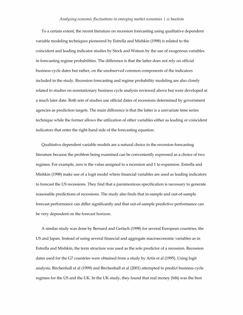
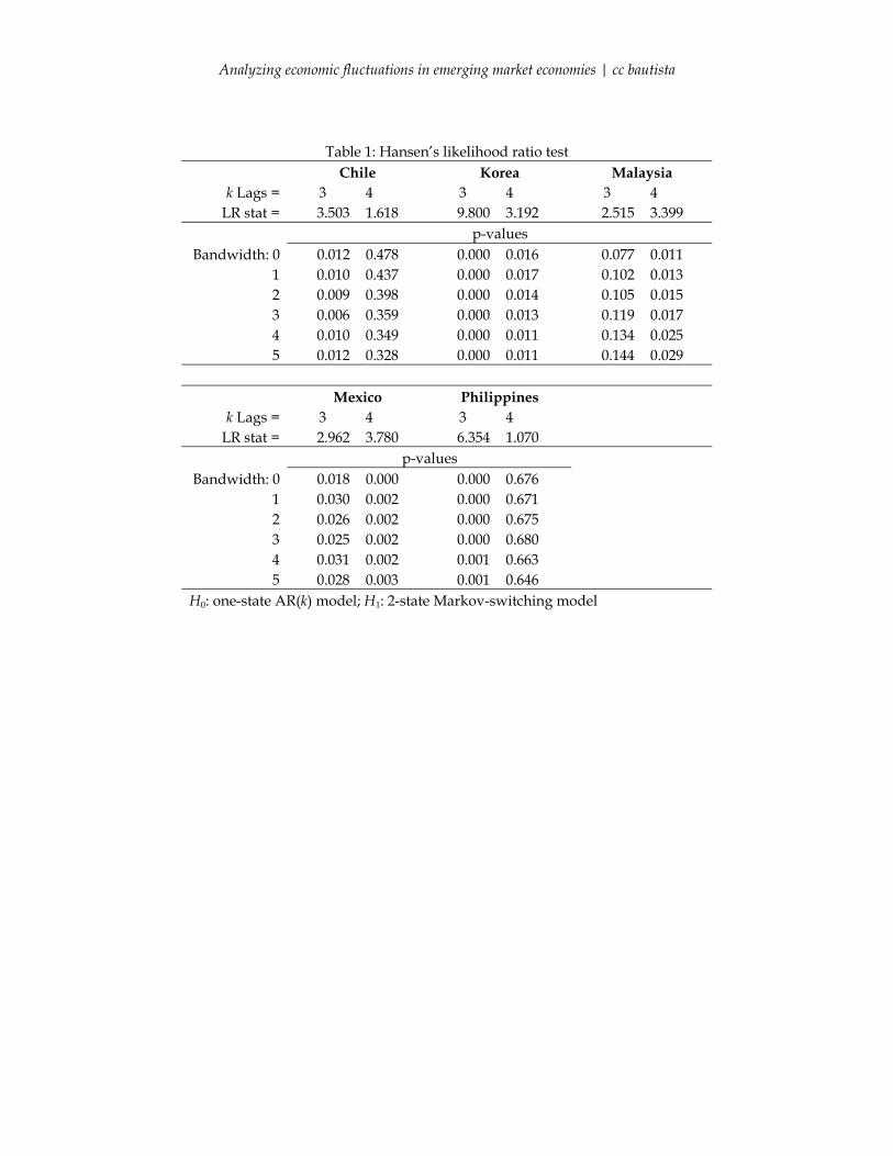
Table 1 shows Hansen’s (1992, 1996) likelihood ratio tests of the null of a one-state AR(k)
model against the alternative of a 2-state Markov regime-switching model. As can be seen, for lag
lengths of 3 and 4, the tests show a rejection of the null hypothesis in most cases. As a
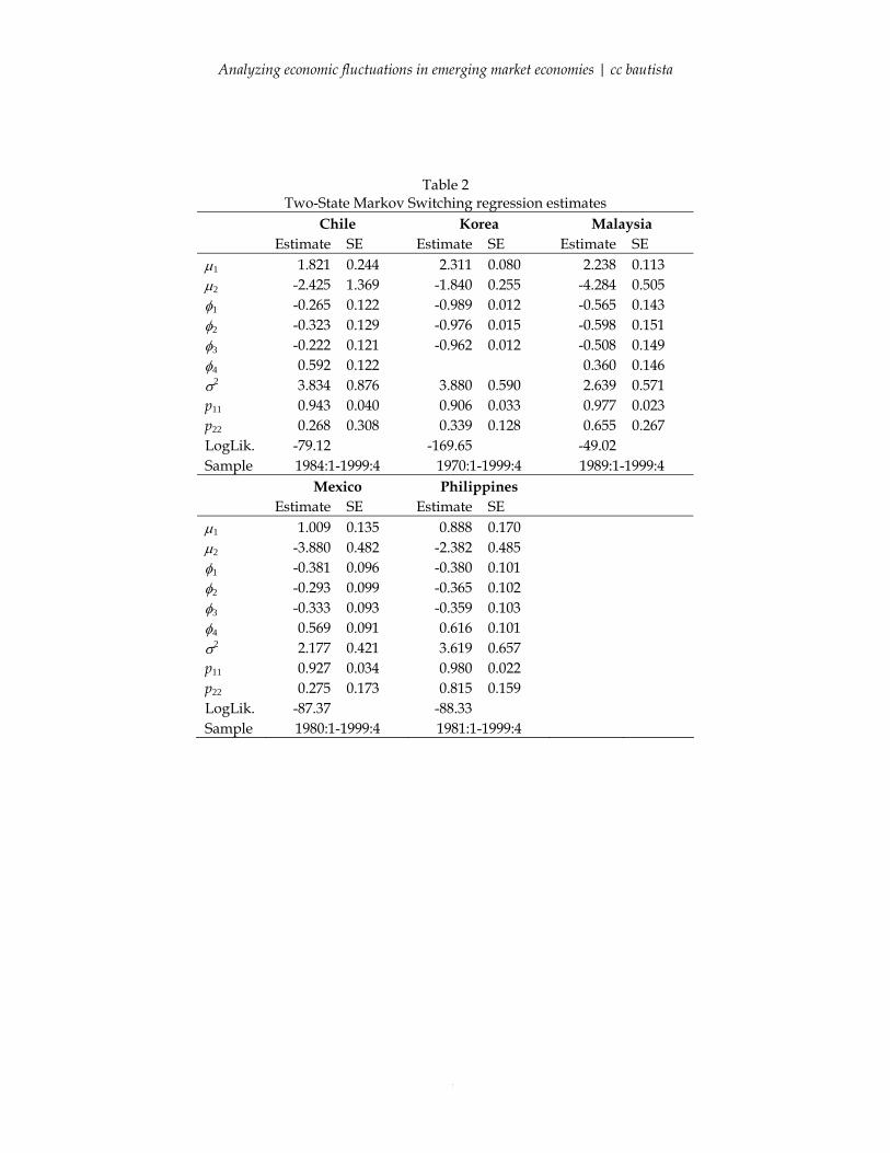
preliminary analysis, 2-state models were estimated and the results are shown in Table 2.
Statistically significant parameter estimates of two-state MS autoregressions for each of the five
countries under study can be seen from the table. It must be note however that 2-state models do
not seem to adequately capture normal movements in economic activity when economic crises
are deep. For example, the impact of the 1983-85 crisis in the Philippines is so huge that it dwarfs
the effects of the Asian crisis, causing a misclassification. These can be observed in Figure 1 which
shows the smoothed probabilities of each state along with actual growth rates using
deseasonalized GDP.
7
Analyzing economic fluctuations in emerging market economies | cc bautista
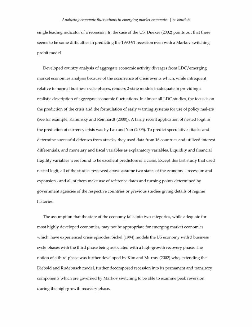
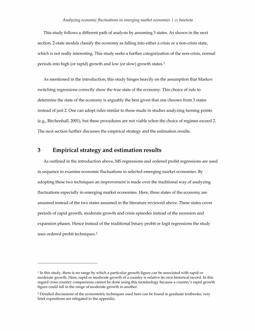
Next, the study proceeds to estimate 3-state MS autoregressions with maximum lag lengths of
4 as in the 2-state models. It is important to note here that because of the highly non-linear nature
of the problem, unrestricted maximum likelihood estimates of 3-state models are more difficult to
obtain. In this regard, some values of parameters that can be reasonably assumed to take on
boundary values were determined. This is not an unusual procedure and has been employed by
Hamilton (2005) in his study of U.S. unemployment. Inspection of the time series reveals that in
most cases, the movements in GDP growth around crisis periods show no abrupt decline from a
position of rapid growth to negative growth which indicates a crisis event. Rather, growth often
slows a bit before going into a crisis episode. This is also true when the economy is coming out of
the crisis – the economy does not shift immediately to a rapid growth path but has to climb
slowly out of the bottom. Hence, letting s = 1 as the state indicating rapid growth, s = 2 indicating
moderate growth and s = 3 representing a crisis state, it seems reasonable to assume that state 1 is
never followed by state 3 and vice versa. More precisely, let pij represent the transition
probabilities. This amounts to an assumption that p13 = p31 = 0.
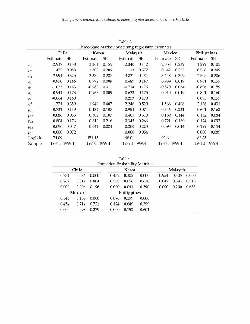
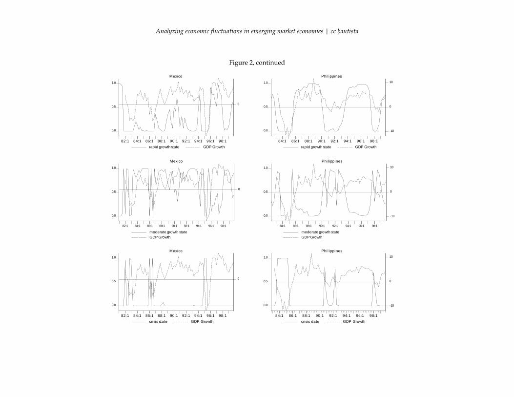
Table 3 reports the results of 3-state MS regression estimates. For each country, unrestricted
maximum likelihood estimates were computed and convergence was obtained for Chile,
Malaysia and the Philippines. The restrictions mentioned above were imposed for Korea and
Mexico in order to attain convergence. Table 4 shows the corresponding transition probability
matrix for each country estimate. To get an idea of how the 3-state MS model tracks economic
activity, Figure 2 plots the smoothed probabilities on the left scale and GDP growth on the right
scale. It is seen that this performs better than the 2-state model.
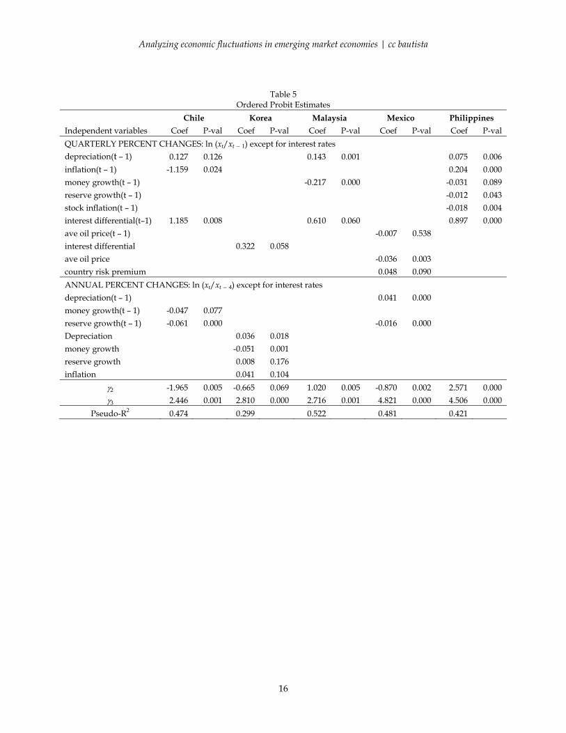
Table 5 presents the estimates of ordered probit models for each country. The study tries to
limit itself to major macroeconomic variables: nominal exchange rate, general price level, money
8
Analyzing economic fluctuations in emerging market economies | cc bautista
supply, and interest rate which appear in all country estimates.3 In some cases however, other
variables which are deemed important to the economy are included, e.g., for Mexico the price of
oil, foreign exchange reserves and country risk premium, defined as the difference between the
interest differential and the actual depreciation rate, were used. Also these variables percent
changes either on a quarterly or annually basis. The final estimates shown in the table were
chosen based on the pseudo-R2 and the significance of the coefficients.
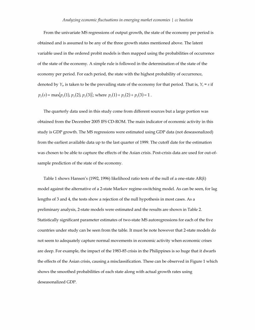
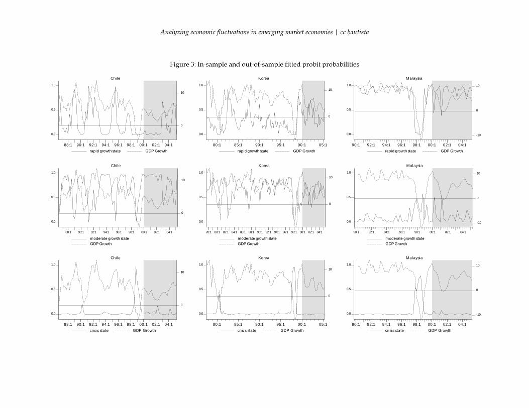
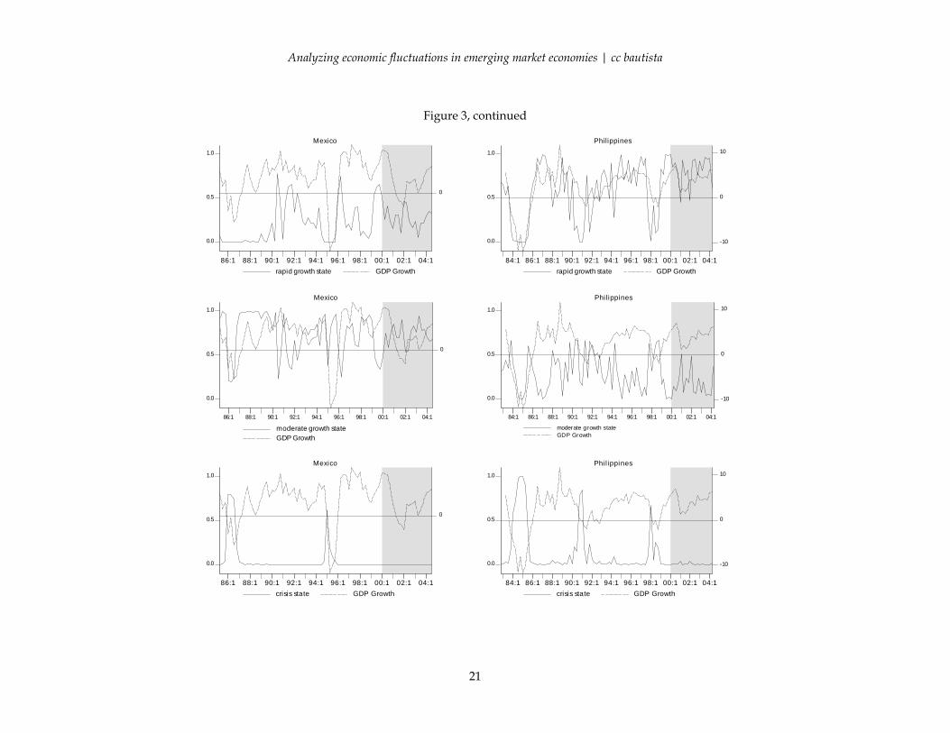
Figure 3 shows the fitted probabilities from the ordered probit estimates. For reference, the
annual GDP growth is also plotted as broken lines. The shaded portion of the graphs covers the
out-of-sample forecasts from 2000 to 2005. It is clear from the diagrams that no crisis events took
place in the countries under study during this period. There are however fluctuations in the
growth patterns in some of them. For Chile for example, the probability of rapid growth is
highest for the first half of 2003 and the last quarter of 2004 and first quarter of 2005. Korea’s
growth pattern shifted between moderate and rapid from 2000 to the end of 2002 and then
remained in moderate growth mode. Malaysia remained at the rapid growth state until it
experienced a slowdown in exports in 2001. This is reflected in the shift from rapid to moderate
growth in the third quarter of that year. For the Philippines, deviations from rapid growth took
place in the first quarter of 2001 when a radical change in the country’s leadership occurred as
seen in the diagram.
4 Concluding remarks
This study has demonstrated that it is possible to adopt econometric tools used to analyze
fluctuations in advanced economies to emerging market economies. The results above show that
the models constructed are able to track the movements of aggregate economic activity fairly well
and have satisfactory out-of-sample performance. This exploratory model building exercise make
3 Unit root tests of these variables are shown in the Appendix.
9

Analyzing economic fluctuations in emerging market economies | cc bautista
use data from five selected emerging market economies. This procedure outlined in this paper
can be adapted to other emerging market economies as well. The models above can be used for
policy analysis because it makes use of macroeconomic variables to track and predict growth. The
results show to some extent the usefulness of these macroeconomic variables in predicting
slowdowns. Also simulations can be done to determine under what combination of values of
these variables can lead to crisis situations – similar to early warning systems. This is not done in
this study but is an area of further research.
10
Analyzing economic fluctuations in emerging market economies | cc bautista
References
Artis M, Kontelemis Z, D Osborn, (1995), Classical business cycles for G7 and European countries, CEPR Discussion Paper 1137.
Bernard H and S Gerlach, (1998), Does the term structure predict recessions? The international evidence, International Journal of Finance and Economics 3, 195-215.
Bautista C, (2003), Estimates of output gaps in four Southeast Asian countries, Economics Letters 80(3), pp. 365-371.
Bautista C, (2002), Boom–bust cycles and crisis periods in the Philippines: A regime–switching Analysis, Philippine Review of Economics.
Birchenhall C, Jessen H, Osborn D and P Simpson, (1999), Predicting U.S. business-cycle regimes, Journal of Business and Economic Statistics 17(3), 313-323.
Birchenhall C, Osborn D and M Sensier, (2001), “Predicting UK business cycle regimes, Scottish Journal of Political Economy 48(2), 179-195
Davidson R and J MacKinnon, (1993), Estimation and Inference in Econometrics, Oxford University Press.
Diebold F and G Rudebusch, (1996), Measuring business cycles: A modern perspective, Review of Economics and Statistics, 67-77
Dueker, M (2002), Regime-dependent forecast and the 2001 recession, Economic Review, Federal Reserve Board of St Louis, 29-36.
Filardo, A, (1994), Business-cycle phases and their transitional dynamics, Journal of Business and Economic Statistics, 299-308.
Hamilton J, (2005), What’s real about the business cycle?, Federal Reserve Bank of St Louis Review, 435-452.
Hamilton J, (1989), A new approach to the economic analysis of nonstationary time series and the business cycle, Econometrica, 357–384.
Hamilton J, and B Raj, (2002), New directions in business cycle research and financial analysis, in Advances in Markov-Switching Models, Hamilton J, and B Raj (eds.), Physica-Verlag.
Hamilton J, and R Susmel, (1994), Autoregressive conditional heteroskedasticity and changes in regime, Journal of Econometrics, 64, 307 – 333.
Hansen, Bruce (1992), “The likelihood ratio test under nonstandard conditions: Testing the Markov switching model of GNP,” Journal of Applied Econometrics 7, S61-S82. Erratum (1996), vol 11, 195-198.
Kaminsky G and C Reinhardt (2000), On crisis, contagion and confusion, Journal of International Economics 51, 145-168.
Kim C-J, (1994), Dynamic linear models with Markov-switching, Journal of Econometrics, 60, 1–22.
Kim C-J and C Murray, (2002), Permanent and transitory components of recessions, in Advances in Markov-Switching Models, Hamilton J, and B Raj (eds.), Physica-Verlag.
Kim C-J and C Nelson, (1999), State-Space Models with Regime Switching, The MIT Press, Cambridge, Massachusetts, USA.
11
Analyzing economic fluctuations in emerging market economies | cc bautista
Krolzig M, (1997), Markov-switching vector autoregressions, modelling, statistical inference and application to business cycle analysis, Lecture Notes in Economics and Mathematical Systems 454, Berlin: Springer.
Lam P-S, (1990), The Hamilton model with a general autoregressive component, Journal of Monetary Economics, 409–432.
Lau L and I Yan, (2005), Predicting currency crisis with a nested logit model, Pacific Economic Review 10(3), 296-316.
Sichel D, (1994), Inventories and the three phases of the business cycle, Journal of Business and Economic Statistics 12, 269–277.
Stock S and M Watson (1992), A procedure for predicting recessions with leading indicators: Econometric issues and recent experience, NBER working paper 4014.
Stock S and M Watson (1988), A probability model of the coincident indicators, NBER working paper 2772.
12
Analyzing economic fluctuations in emerging market economies | cc bautista
Table 1: Hansen’s likelihood ratio test Chile Korea Malaysia
k Lags = 3 4 3 4 3 4 LR stat = 3.503 1.618 9.800 3.192 2.515 3.399
p-values Bandwidth: 0 0.012 0.478 0.000 0.016 0.077 0.011
1 0.010 0.437 0.000 0.017 0.102 0.013 2 0.009 0.398 0.000 0.014 0.105 0.015 3 0.006 0.359 0.000 0.013 0.119 0.017 4 0.010 0.349 0.000 0.011 0.134 0.025 5 0.012 0.328 0.000 0.011 0.144 0.029
Mexico Philippines
k Lags = 3 4 3 4 LR stat = 2.962 3.780 6.354 1.070
p-values Bandwidth: 0 0.018 0.000 0.000 0.676
1 0.030 0.002 0.000 0.671 2 0.026 0.002 0.000 0.675 3 0.025 0.002 0.000 0.680 4 0.031 0.002 0.001 0.663 5 0.028 0.003 0.001 0.646
H0: one-state AR(k) model; H1: 2-state Markov-switching model
13
Analyzing economic fluctuations in emerging market economies | cc bautista
Table 2 Two-State Markov Switching regression estimates
Chile Korea Malaysia Estimate SE Estimate SE Estimate SE μ1 1.821 0.244 2.311 0.080 2.238 0.113 μ2 -2.425 1.369 -1.840 0.255 -4.284 0.505 φ1 -0.265 0.122 -0.989 0.012 -0.565 0.143 φ2 -0.323 0.129 -0.976 0.015 -0.598 0.151 φ3 -0.222 0.121 -0.962 0.012 -0.508 0.149 φ4 0.592 0.122 0.360 0.146 σ2 3.834 0.876 3.880 0.590 2.639 0.571 p11 0.943 0.040 0.906 0.033 0.977 0.023 p22 0.268 0.308 0.339 0.128 0.655 0.267 LogLik. -79.12 -169.65 -49.02 Sample 1984:1-1999:4 1970:1-1999:4 1989:1-1999:4 Mexico Philippines Estimate SE Estimate SE μ1 1.009 0.135 0.888 0.170 μ2 -3.880 0.482 -2.382 0.485 φ1 -0.381 0.096 -0.380 0.101 φ2 -0.293 0.099 -0.365 0.102 φ3 -0.333 0.093 -0.359 0.103 φ4 0.569 0.091 0.616 0.101 σ2 2.177 0.421 3.619 0.657 p11 0.927 0.034 0.980 0.022 p22 0.275 0.173 0.815 0.159 LogLik. -87.37 -88.33 Sample 1980:1-1999:4 1981:1-1999:4
14
Analyzing economic fluctuations in emerging market economies | cc bautista
Table 3 Three-State Markov Switching regression estimates
Chile Korea Malaysia Mexico Philippines Estimate SE Estimate SE Estimate SE Estimate SE Estimate SE μ1 2.937 0.150 3.361 0.155 2.340 0.112 2.058 0.239 1.299 0.105 μ2 1.477 0.088 1.302 0.209 1.113 0.577 0.642 0.225 0.568 0.349 μ3 -2.994 0.325 -3.330 0.287 -3.831 0.481 -3.448 0.309 -2.505 0.206 φ1 -0.970 0.166 -0.992 0.009 -0.687 0.167 -0.939 0.049 -0.901 0.157 φ2 -1.023 0.163 -0.980 0.011 -0.714 0.176 -0.870 0.064 -0.896 0.159 φ3 -0.944 0.173 -0.966 0.009 -0.633 0.175 -0.910 0.049 -0.891 0.160 φ4 -0.064 0.160 0.253 0.170 0.095 0.157 σ2 1.721 0.359 1.949 0.407 2.246 0.529 1.566 0.408 2.136 0.431 p11 0.731 0.139 0.432 0.107 0.954 0.074 0.546 0.231 0.601 0.162 p12 0.086 0.053 0.302 0.107 0.405 0.310 0.189 0.144 0.152 0.084 p23 0.804 0.176 0.610 0.216 0.345 0.266 0.721 0.169 0.124 0.093 p32 0.096 0.047 0.041 0.024 0.200 0.223 0.098 0.044 0.199 0.154 p31 0.000 0.072 0.000 0.054 0.000 0.089 LogLik. -74.09 -154.15 -48.01 -93.64 -86.35 Sample 1984:1-1999:4 1970:1-1999:4 1989:1-1999:4 1980:1-1999:4 1981:1-1999:4
Table 4 Transition Probability Matrices
Chile Korea Malaysia 0.731 0.086 0.000 0.432 0.302 0.000 0.954 0.405 0.000 0.269 0.819 0.804 0.568 0.656 0.610 0.047 0.394 0.345 0.000 0.096 0.196 0.000 0.041 0.390 0.000 0.200 0.655
Mexico Philippines 0.546 0.189 0.000 0.876 0.199 0.000 0.454 0.714 0.721 0.124 0.649 0.399 0.000 0.098 0.279 0.000 0.152 0.601
15
Analyzing economic fluctuations in emerging market economies | cc bautista
16
Table 5 Ordered Probit Estimates
Chile Korea Malaysia Mexico Philippines Independent variables Coef P-val Coef P-val Coef P-val Coef P-val Coef P-val QUARTERLY PERCENT CHANGES: ln (xt/xt – 1) except for interest rates depreciation(t – 1) 0.127 0.126 0.143 0.001 0.075 0.006 inflation(t – 1) -1.159 0.024 0.204 0.000 money growth(t – 1) -0.217 0.000 -0.031 0.089 reserve growth(t – 1) -0.012 0.043 stock inflation(t – 1) -0.018 0.004 interest differential(t–1) 1.185 0.008 0.610 0.060 0.897 0.000 ave oil price(t – 1) -0.007 0.538 interest differential 0.322 0.058 ave oil price -0.036 0.003 country risk premium 0.048 0.090 ANNUAL PERCENT CHANGES: ln (xt/xt – 4) except for interest rates depreciation(t – 1) 0.041 0.000 money growth(t – 1) -0.047 0.077 reserve growth(t – 1) -0.061 0.000 -0.016 0.000 Depreciation 0.036 0.018 money growth -0.051 0.001 reserve growth 0.008 0.176 inflation 0.041 0.104
γ2 -1.965 0.005 -0.665 0.069 1.020 0.005 -0.870 0.002 2.571 0.000 γ3 2.446 0.001 2.810 0.000 2.716 0.001 4.821 0.000 4.506 0.000
Pseudo-R2 0.474 0.299 0.522 0.481 0.421
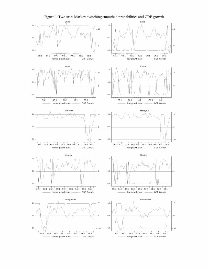
Figure 1: Two-state Markov switching smoothed probabilities and GDP growth
0.0
0.5
1.0
0
10
86:1 88:1 90:1 92:1 94:1 96:1 98:1normal growth state GDP Growth
Chile
0.0
0.5
1.0
0
10
86:1 88:1 90:1 92:1 94:1 96:1 98:1low growth state GDP Growth
Chile
0.0
0.5
1.0
0
10
75:1 80:1 85:1 90:1 95:1normal growth state GDP Growth
Korea
0.0
0.5
1.0
0
10
75:1 80:1 85:1 90:1 95:1low growth state GDP Growth
Korea
0.0
0.5
1.0
-10
0
10
90:1 91:1 92:1 93:1 94:1 95:1 96:1 97:1 98:1 99:1normal growth state GDP Growth
Malaysia
0.0
0.5
1.0
-10
0
10
90:1 91:1 92:1 93:1 94:1 95:1 96:1 97:1 98:1 99:1low growth state GDP Growth
Malaysia
0.0
0.5
1.0
0
82:1 84:1 86:1 88:1 90:1 92:1 94:1 96:1 98:1normal growth state GDP Growth
Mexico
0.0
0.5
0.0
0.5
1.0
1.0
0
82:1 84:1 86:1 88:1 90:1 92:1 94:1 96:1 98:1low growth state GDP Growth
Mexico
-10
0
84:1 86:1
10
88:1 90:1 92:1 94:1 96:1 98:1normal growth state GDP Growth
Phil ippines
0.0
0.5
1.0
-10
0
84:1 86:1
10
88:1 90:1 92:1 94:1 96:1 98:1low growth state GDP Growth
Phil ippines
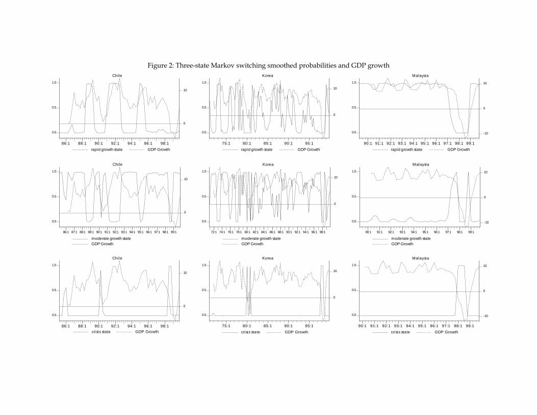
Figure 2: Three-state Markov switching smoothed probabilities and GDP growth
0.0
0.5
1.0
0
10
86:1 88:1 90:1 92:1 94:1 96:1 98:1rapid growth state GDP Growth
Chile
0.0
0.5
1.0
0
10
75:1 80:1 85:1 90:1 95:1rapid growth state GDP Growth
Korea
0.0
0.5
1.0
-10
0
10
90:1 91:1 92:1 93:1 94:1 95:1 96:1 97:1 98:1 99:1rapid growth state GDP Growth
Malaysia
0.0
0.5
1.0
0
10
86:1 87:1 88:1 89:1 90:1 91:1 92:1 93:1 94:1 95:1 96:1 97:1 98:1 99:1
moderate growth stateGDP Growth
Chile
0.0
0.5
1.0
0
10
72:1 74:1 76:1 78:1 80:1 82:1 84:1 86:1 88:1 90:1 92:1 94:1 96:1 98:1
moderate growth stateGDP Growth
Korea
0.0
0.5
1.0
-10
0
10
90:1 91:1 92:1 93:1 94:1 95:1 96:1 97:1 98:1 99:1
moderate growth stateGDP Growth
Malaysia
0.0
0.5
1.0
0
10
86:1 88:1 90:1 92:1 94:1 96:1 98:1crisis state GDP Growth
Chile
0.0
0.5
1.0
0
10
75:1 80:1 85:1 90:1 95:1crisis state GDP Growth
Korea
0.0
0.5
1.0
-10
0
10
90:1 91:1 92:1 93:1 94:1 95:1 96:1 97:1 98:1 99:1crisis state GDP Growth
Malaysia
Analyzing economic fluctuations in emerging market economies | cc bautista
Figure 2, continued
0.0
0.5
1.0
0
82:1 84:1 86:1 88:1 90:1 92:1 94:1 96:1 98:1rapid growth state GDP Growth
Mexico
0.0
0.5
1.0
-10
0
10
84:1 86:1 88:1 90:1 92:1 94:1 96:1 98:1rapid growth state GDP Growth
Philippines
0.0
0.5
1.0
0
82:1 84:1 86:1 88:1 90:1 92:1 94:1 96:1 98:1
moderate growth stateGDP Growth
Mexico
0.0
0.5
1.0
-10
0
10
84:1 86:1 88:1 90:1 92:1 94:1 96:1 98:1
moderate growth stateGDP Growth
Philippines
0.0
0.5
1.0
0
82:1 84:1 86:1 88:1 90:1 92:1 94:1 96:1 98:1crisis state GDP Growth
Mexico
0.0
0.5
1.0
-10
0
10
84:1 86:1 88:1 90:1 92:1 94:1 96:1 98:1crisis state GDP Growth
Phil ippines
19
Analyzing economic fluctuations in emerging market economies | cc bautista
Figure 3: In-sample and out-of-sample fitted probit probabilities
0.0
0.5
1.0
0
10
88:1 90:1 92:1 94:1 96:1 98:1 00:1 02:1 04:1rapid growth state GDP Growth
Chile
0.0
0.5
1.0
0
10
80:1 85:1 90:1 95:1 00:1 05:1rapid growth state GDP Growth
Korea
0.0
0.5
1.0
-10
0
10
90:1 92:1 94:1 96:1 98:1 00:1 02:1 04:1rapid growth state GDP Growth
Malaysia
0.0
0.5
1.0
0
10
88:1 90:1 92:1 94:1 96:1 98:1 00:1 02:1 04:1
moderate growth stateGDP Growth
Chile
0.0
0.5
1.0
0
10
78:1 80:1 82:1 84:1 86:1 88:1 90:1 92:1 94:1 96:1 98:1 00:1 02:1 04:1
moderate growth stateGDP Growth
Korea
0.0
0.5
1.0
-10
0
10
90:1 92:1 94:1 96:1 98:1 00:1 02:1 04:1
moderate growth stateGDP Growth
Malaysia
0.0
0.5
1.0
0
10
88:1 90:1 92:1 94:1 96:1 98:1 00:1 02:1 04:1crisis state GDP Growth
Chile
0.0
0.5
1.0
0
10
80:1 85:1 90:1 95:1 00:1 05:1crisis state GDP Growth
Korea
0.0
0.5
1.0
-10
0
10
90:1 92:1 94:1 96:1 98:1 00:1 02:1 04:1crisis state GDP Growth
Malaysia
20
Analyzing economic fluctuations in emerging market economies | cc bautista
21
0.0
0.5
1.0
0
86:1 88:1 90:1 92:1 94:1 96:1 98:1 00:1 02:1 04:1rapid growth state GDP Growth
Mexico
0.0
0.5
1.0
-10
0
10
84:1 86:1 88:1 90:1 92:1 94:1 96:1 98:1 00:1 02:1 04:1rapid growth state GDP Growth
Philippines
0.0
0.5
1.0
0
86:1 88:1 90:1 92:1 94:1 96:1 98:1 00:1 02:1 04:1
moderate growth stateGDP Growth
Mexico
0.0
0.5
1.0
-10
0
10
84:1 86:1 88:1 90:1 92:1 94:1 96:1 98:1 00:1 02:1 04:1
moderate growth stateGDP Growth
Philippines
0.0
0.5
1.0
0
86:1 88:1 90:1 92:1 94:1 96:1 98:1 00:1 02:1 04:1crisis state GDP Growth
Mexico
0.0
0.5
1.0
-10
0
10
84:1 86:1 88:1 90:1 92:1 94:1 96:1 98:1 00:1 02:1 04:1crisis state GDP Growth
Phil ippines
Figure 3, continued
Appendix
Markov-Switching Regression
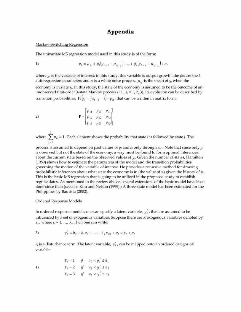
The univariate MS regression model used in this study is of the form:
1) ( ) ( ) tsktkstst ktttyyy εμφμφμ +−++−+=
−− −− ...111
where yt is the variable of interest; in this study, this variable is output growth; the φks are the k autoregression parameters and εt is a white noise process. is the mean of y
tsμ t when the economy is in state st. In this study, the state of the economy is assumed to be the outcome of an unobserved first-order 3-state Markov process (i.e., st = 1, 2, 3). Its evolution can be described by transition probabilities, ( ) ijtt pisjs === − 1Pr , that can be written in matrix form:
2) ⎥⎥⎥
⎦
⎤
⎢⎢⎢
⎣
⎡=
332313
332212
312111
ppppppppp
P
where . Each element shows the probability that state i is followed by state j. The
process is assumed to depend on past values of y
∑=
=3
1
1j
ijp
t and st only through st–1. Note that since only yt is observed but not the state of the economy, a way must be found to form optimal inferences about the current state based on the observed values of yt. Given the number of states, Hamilton (1989) shows how to estimate the parameters of the model and the transition probabilities governing the motion of the variable of interest. He provides a recursive method for drawing probabilistic inferences about what state the economy is in (the value of st) given the history of yt. This is the basic MS regression that is going to be utilized in the proposed study to establish regime dates. As mentioned in the review above, several extensions of the basic model have been done since then (see also Kim and Nelson (1999).) A three-state model has been estimated for the Philippines by Bautista (2002).
Ordered Response Models
In ordered response models, one can specify a latent variable, , that are assumed to be *ty
influenced by a set of exogenous variables. Suppose there are K exogenous variables denoted by xkt, where k = 1, …, K. Then one can write:
3) tttKtKtt zxbxbby εε +=++++= ...110*
εt is a disturbance term. The latent variable, , can be mapped onto an ordered categorical *ty
variable:
4)
3*
2
2*
1
1*
0
3
2
1
ayaifY
ayaifY
ayaifY
tt
tt
tt
≤<=
≤<=
≤<=

Analyzing economic fluctuations in emerging market economies | cc bautista
where a0, a1, a2 and a3 are thresholds that serve to determine the value of Yt to be given to the latent variable. To preserve the ordering, these thresholds that are to be estimated econometrically along with the coefficients of equation (4) must satisfy: a0 > a1 > a2 > a3. The latent variable’s boundary values are unknown. Hence, one can simply set the beginning and ending thresholds to minus and plus infinity respectively (in this case, a0 = –∞ and a3 = +∞) and need not be estimated. From the above expressions, one can write the ordered regression model as:
5)
( ) ( )( )
( ) ( )( ) ( )
( ) ( )( )t
ttKttt
tt
tttKttt
t
ttKttt
zaFzaxxY
zaFzaFzazaxxY
zaFzaxxY
−−=
−≥==
−−−=
−≤<−==
−=
−≤==
2
21
12
211
1
11
1Pr...,,3Pr
Pr...,,2Pr
Pr...,,1Pr
ε
ε
ε
where F denotes the cumulative distribution function of ε. Let there be a total of T sample periods, (t = 1, …, T), each of which can be treated as a single draw from a multinomial distribution. Suppose T1, T2 and T3 are the number of periods belonging to states 1, 2 and 3 respectively, with T1 +T2 + T3= T. Then the likelihood of observing the sample is given by:
6) ( ) ( ) ( )[ ] [ ( )] 3212121 1 T
tT
ttT
t zaFzaFzaFzaFL −−−−−−=
The parameters of the model, the ah’s and the bk’s, can be estimated by maximizing the (log of the) likelihood function given by equation (6). can be computed once the b coefficients are tzestimated. With estimates of the limit coefficients, , and , the probability of being at a sahˆ tzparticular state can be predicted for each period t in the sample:
7)
( )
( ) ( )
( )tt
ttt
tt
zaFp
zaFzaFp
zaFp
ˆˆ1ˆ
ˆˆˆˆˆ
ˆˆˆ
23
122
11
−−=
−−−=
−=
where . The disturbance term, ε1ˆˆˆ 321 =++ ttt ppp t, can be assumed to follow a normal or a logistic distribution to produce either the ordered probit or the ordered logit model, respectively. A good reference on qualitative and limited dependent variables regression like the above is Davidson and MacKinnon (1993). Ordered probit and logit models are known to be well-behaved and are easily implemented using commercially available econometric programs.
23