Embed Size (px)
Citation preview
Business Cycles in Emerging Markets: The Role
of Durable Goods and Financial Frictions
Fernando Alvarez-Parra, Luis Brandao Marques, and
Manuel Toledo
WP/11/133
© 2011 International Monetary Fund WP/11/133
IMF Working Paper
IMF Institute
Business Cycles in Emerging Markets: The Role of Durable Goods and Financial Frictions
Prepared by Fernando Alvarez-Parra, Luis Brandao Marques, and Manuel Toledo1
Authorized for distribution by Jorge Roldós
June 2011
Abstract
This paper examines how durable goods and financial frictions shape the business cycle of
a small open economy subject to shocks to trend and transitory shocks. In the data,
nondurable consumption is not as volatile as income for both developed and emerging
market economies. The simulation of the model implies that shocks to trend play a less
important role than previously documented. Financial frictions improve the ability of the
model to match some key business cycle properties of emerging economies. A
countercyclical borrowing premium interacts with the nature of durable goods delivering
highly volatile consumption and very countercyclical net exports.
JEL Classification Numbers: E32, F41, F47.
Keywords: emerging markets, real business cycles, durables, financial frictions.
Author’s E-Mail Address: [email protected], [email protected], and [email protected].
This Working Paper should not be reported as representing the views of the IMF. The views expressed in this Working Paper are those of the author(s) and do not necessarily
represent those of CAF, the IMF or IMF policy. Working Papers describe research in progress by
the author(s) and are published to elicit comments and to further debate.
1 Alvarez-Parra is research economist at the Corporación Andina de Fomento, Brandao Marques is senior
economist at the IMF Institute, and Toledo is assistant professor at Universidad Carlos III de Madrid. The authors
thank Pravin Krishna, Jorge Roldós, and Mico Loretan for helpful comments. Toledo is grateful to the Spanish
Ministry of Science and Innovation for financial support through grant Juan de la Cierva.
2
Contents Page
I. Introduction . . . . . . . . . . . . . . . . . . . . . . . . . . . . . . . . . . . . . . 4
II. Data and Stylized Facts . . . . . . . . . . . . . . . . . . . . . . . . . . . . . . . . 6A. Data . . . . . . . . . . . . . . . . . . . . . . . . . . . . . . . . . . . . . . . . 6B. Facts . . . . . . . . . . . . . . . . . . . . . . . . . . . . . . . . . . . . . . . 7
III. The model . . . . . . . . . . . . . . . . . . . . . . . . . . . . . . . . . . . . . . . 9
IV. Calibration . . . . . . . . . . . . . . . . . . . . . . . . . . . . . . . . . . . . . . . 14
V. Results . . . . . . . . . . . . . . . . . . . . . . . . . . . . . . . . . . . . . . . . . 15A. No Financial Frictions Case . . . . . . . . . . . . . . . . . . . . . . . . . . . 16B. Financial Frictions Case . . . . . . . . . . . . . . . . . . . . . . . . . . . . . 19C. Robustness . . . . . . . . . . . . . . . . . . . . . . . . . . . . . . . . . . . . 21
VI. Conclusions . . . . . . . . . . . . . . . . . . . . . . . . . . . . . . . . . . . . . . 22
Appendix
A. Additional Derivations . . . . . . . . . . . . . . . . . . . . . . . . . . . . . . . . . 25A.1. Equivalent planner’s problem . . . . . . . . . . . . . . . . . . . . . . . . . . . 25
A.1.1. First order conditions . . . . . . . . . . . . . . . . . . . . . . . . . . . 26A.1.2. Envelope conditions . . . . . . . . . . . . . . . . . . . . . . . . . . . . 26
A.2. Steady-state relationships . . . . . . . . . . . . . . . . . . . . . . . . . . . . . 27A.3. Tradability assumption . . . . . . . . . . . . . . . . . . . . . . . . . . . . . . 27
References . . . . . . . . . . . . . . . . . . . . . . . . . . . . . . . . . . . . . . . . . . 29
Figures
1. Relative Volatility of Consumption and Saving Rates Across Countries . . . . . . . 312. Effect of Shocks to Trend on Key Moments . . . . . . . . . . . . . . . . . . . . . . 313. Impulse-Response Functions for a Permanent Shock . . . . . . . . . . . . . . . . . 324. Impulse-Response Functions for a Shock to Nondurables . . . . . . . . . . . . . . 325. Impulse-Response Functions for a Shock to Durables . . . . . . . . . . . . . . . . 336. Effect of Financial Frictions on Key Moments . . . . . . . . . . . . . . . . . . . . 33
Tables
1. Volatility of Output and Relative Volatility of Consumption, Investment and NetExports . . . . . . . . . . . . . . . . . . . . . . . . . . . . . . . . . . . . . . . . . 34
2. Correlations with Output . . . . . . . . . . . . . . . . . . . . . . . . . . . . . . . . 353. Average Relative Volatility of Consumption. . . . . . . . . . . . . . . . . . . . . . 354. Benchmark Parameter Values. . . . . . . . . . . . . . . . . . . . . . . . . . . . . . 365. Simulated moments and parameter estimates for Mexico . . . . . . . . . . . . . . . 37

3
6. Simulated moments and parameter estimates for an alternative specifications ofthe borrowing premium . . . . . . . . . . . . . . . . . . . . . . . . . . . . . . . . 38
4
I. INTRODUCTION
The business cycle in emerging market economies is characterized by a strongly countercycli-cal current account and by sovereign interest rates which are also highly countercyclical, veryvolatile, and significantly higher than the World interest rate. In addition, total consumptionexpenditure volatility exceeds income volatility. Aguiar and Gopinath (2007) report that con-sumption is 40 percent more volatile than income for emerging economies, while slightly lessvolatility than income for developed economies. This fact is known as the excess volatility of
consumption puzzle.
The ultimate goal of this paper is to explore possible explanations for business cycle reg-ularities observed in emerging market economies when considering the existence of bothconsumer durable and nondurable goods. For this effect, we build a model which combinesshocks to trend and shocks to cycle (Aguiar and Gopinath, 2007) with financial frictionsand durable goods. The disaggregation of consumption into durable and nondurable goodsimposes some discipline to our calibration exercises and creates a channel through whichshocks can deliver more countercyclical net exports and more volatile expenditure in durablegoods. We calibrate the model to match key business cycle facts for Mexico.
One leading explanation for these regularities relies on shocks to trend growth. Aguiar andGopinath (2007) find that a standard equilibrium model is consistent with the cyclical proper-ties of emerging economies once the income process incorporates shocks to trend in additionto transitory fluctuations around the trend. The intuition comes from the permanent incomehypothesis: a change in the trend of income implies a stronger response of consumption thana transitory fluctuation around the trend. They conclude that the business cycle in emergingeconomies is principally driven by shocks to trend growth. However, we show this result doesnot hold once we add durable goods to the consumption bundle.
Limited access to international borrowing and other shocks which directly or indirectly affectexternal interest rates have also been used as an explanations for the puzzle. This is a naturaldriving force because empirical findings indicate a strong relation between sovereign inter-est rates and output. In early real business cycle models for small open economies, interestrates disturbances play a minor role in driving the business cycle (Mendoza, 1991). When oneadds endogenous borrowing limits to a model of a small open economy, however, consump-tion volatility increases substantially as savings cannot be used to smooth consumption whenthe borrowing limit binds (De Resende, 2006). Alternatively, the excessive volatility of con-sumption can be explained with a financial friction in the form of a working capital borrowing
5
requirement (Neumeyer and Perri, 2005). In this case, a countercyclical borrowing premiumamplifies the variability of consumption because it makes the demand for labor more sensitiveto the interest rate. Furthermore, shocks to the volatility of the borrowing premium also playa significant role in explaining the volatility of consumption in emerging market economies(Fernández-Villaverde, Guerrón-Quintana, Rubio-Ramírez, and Uribe, 2009).1 None of thesepapers, however, consider durable goods.
Other papers in the literature study the importance of durables in shaping business cycles insmall open economies. For instance, De Gregorio, Guidotti, and Vegh (1998) study inflationstabilization programs in emerging market economies and the consumption of durable goods.There, a boom-recession cycle in consumption is generated through the wealth effect associ-ated with disinflation (in a cash-in-advance economy) and the existence of non-convex adjust-ment costs for the purchase of durables. For the large open economy case, Engel and Wang(2011) present a two-country model with durables and nondurables and use it to study thevolatility and cyclicality of exports and imports in the United States. Just as we do, they alsoexploit the fact that, while durables are mostly tradable, nondurables are not. Neither De Gre-gorio, Guidotti, and Vegh nor Engel and Wang, however, explore the joint role of financialfrictions and durable goods in shaping emerging markets business cycles.2
Besides Aguiar and Gopinath (2007), our paper relates most to Neumeyer and Perri (2005)and to García-Cicco, Pancrazi, and Uribe (2010). Unlike the latter two, however, we stress theimportance of financial frictions in the presence of durable goods. The interaction betweenfinancial frictions and durable goods is important in explaining the dynamics of emergingmarkets’ business cycles. This is so because the flow of services coming from the stock ofdurables yields utility over time; as a consequence, at least part of the purchase of durablesthat take place today can be seen as postponed consumption (i.e., saving).3 Therefore, thepurchase of durable consumption goods should response strongly to the interest rate. If thelatter is countercyclical, an economic expansion caused by a temporary income shock willencourage consumers to borrow from abroad to take advantage of better credit conditions andthus finance the acquisition of durables. This generates highly volatile purchases of durablesand a strongly countercyclical trade balance.
1There are other explanations for the emerging market consumption volatility puzzle which are not exploredhere. For instance, Boz, Daude, and Durdu (2008) extend Aguiar and Gopinath’s (2007) model to include imper-fect information and Restrepo-Echevarria (2008) explores the role of the informal economy.
2It is true that the wealth effect created by falling inflation present in De Gregorio, Guidotti, and Vegh’swork can be understood as a type of financial friction. Their model, however, only applies to exchange rate-based stabilization programs and not to emerging markets’ business cycles in general.
3A similar hypothesis has been tested, for instance, by Rosenzweig and Wolpin (1993), according to whom,farmers in India use a durable capital good (bullocks) as the primary vehicle for saving and dissaving.
6
The present paper enhances our understanding of business cycles in emerging markets. Interms of empirical regularities we find that, after decomposing consumption into durables andnondurables, the excess volatility of consumption puzzle is explained away in the sense thatnondurable consumption is not more volatile than income either in emerging or in developedeconomies. In particular, we find that the ratio of the standard deviation of nondurable con-sumption relative to that of income is 0.9, for a sample of emerging economies, and 0.72,for a sample of developed economies. Furthermore, our quantitative exercises show that,with durable and nondurable goods, the role played by shocks to trend as a driving force forthe cycle in emerging economies seems smaller than what is found in Aguiar and Gopinath(2007). We show that a financial friction in the form of a countercyclical borrowing pre-mium (in the sense of the induced country risk hypothesis suggested by Neumeyer and Perri,2005) vastly improves the model’s ability to match the key business cycle moments in Mex-ico while, at the same, greatly reduces the importance of shocks to trend. So, at this stage, wecan claim that in order to account for the main characteristics of business cycles in developingeconomies we need to consider explicit financial frictions and not rely only on the propertiesof the technology shocks affecting the economy.
The rest of the paper is organized as follows. In the next section, we present some stylizedfacts about business cycles in open economies. In Section III, we set up a dynamic equilib-rium model where preferences are defined over nondurables, durables, and leisure, and wheretechnological shocks include an aggregate shock to trend and two sector-specific shocks tothe cycle. Section IV describes the calibration procedure and Section V presents the results.Section VI concludes.
II. DATA AND STYLIZED FACTS
A. Data
Our sample is restricted to the countries for which we are able to find data on durable goods’spending. We split the sample into developed and emerging market economies placing in thelatter group the ones rated as such by MSCI for most of the sample period.4 We then dividethe sub-sample of developed economies into two groups according to size and follow the rule
4This criterion means that we include Israel as an emerging market economy since, for the entire sampleperiod it was defined as such by MSCI and only recently upgraded to advanced economy status (May 2010). Thecriterion also means we include the Czech Republic in the pool of emerging market economies in spite of theIMF’s World Economic Outlook having upgraded this country to advanced economy status, in April 2009 (afterthe end of our sample period).
7
that an economy is large if its GDP represented at least 2% of the world’s GDP from 2001 till2008 (period for which we had data for all developed economies). This leaves us with threegroups: small developed economies (Canada, Denmark, Finland, Netherlands, New Zealand,and Spain), large developed economies (France, Italy, Japan, United Kingdom, and UnitedStates), and emerging market economies (Chile, Colombia, Czech Republic, Israel, Mexico,Taiwan Province of China, and Turkey). For each country we collect data (in real terms) ongross domestic product, total private consumption expenditure, consumption of nondurablegoods, expenditure in durable goods, investment, and the trade balance. All data is quarterly,except for Colombia for which it is annual. Sample sizes vary and are detailed in Tables 1 and2.
Our data come from a variety of sources. For the developed economies and the Czech Repub-lic, all data is from the OECD’s Quarterly National Accounts, except for the U.S., for which itis from the Bureau of Economic Analysis. For Chile, data is from Central Bank of Chile. Datafor Colombia comes from DANE - Departamento Administrativo Nacional de Estadística.Data for Israel is from the Bank of Israel and the Central Bureau of Statistics. Mexican datacomes from INEGI - Instituto Nacional de Estadística y Geografía. For Taiwan Province ofChina, we retrieve the data from National Statistics, Republic of China (Taiwan). Finally, forTurkey we use data from the Turkish Statistical Institute. All variables are seasonally adjustedwhen needed, converted to logs and detrended using the Hoddrick-Prescott filter.
B. Facts
When it comes to emerging market economies and small open developed economies, the fol-lowing stylized facts about the business cycle are often cited in the literature (see Aguiar andGopinath, 2007; Neumeyer and Perri, 2005; Uribe and Yue, 2006, and García-Cicco, Pan-crazi, and Uribe, 2010):
1. Real interest rates are countercyclical and leading in emerging markets and acyclicaland lagging in developed economies;
2. Emerging market economies have higher volatilities of output and consumption whencompared to developed economies;
3. Consumption expenditure is more volatile than output in emerging markets while it isnot (quite) as volatile as output in developed economies;
8
4. Net exports are more volatile and more countercyclical in emerging markets when com-pared to developed economies.
To these facts we add the following concerning spending in nondurables and durable goods,based on our sample:
• Consumption of nondurables is not more volatile than output in either small open econ-omies or emerging markets. We find that the ratio of standard deviation of consumption-to income is 0.9, for a sample of emerging economies, and 0.72, for a sample of devel-oped economies (see Table 3);
• Spending in durable goods is much more volatile than output in both sets of economies;
• Overall, consumption spending in both durables and nondurables is relatively morevolatile in emerging markets than in developed economies.
Looking at the data in Table 1 in more detail, it becomes apparent that the relative volatili-ties of total consumption spending (i.e., the ratio of the standard deviation of consumptionto the standard deviation of GDP) and of nondurable consumption show considerable varia-tion within each group. In the case of the emerging market economies, we have Chile, Israel,and Turkey at the high end and Taiwan Province of China, Colombia, and the Czech Repub-lic at the low end.5 While the low value (1.02 for total consumption and 0.81 for nondurableconsumption) of Colombia can be attributed to the annual frequency at which the data issampled, the values for Taiwan Province of China (0.80 and 0.92, respectively) and the CzechRepublic (0.98 and 0.88, respectively) deserve further exploration.
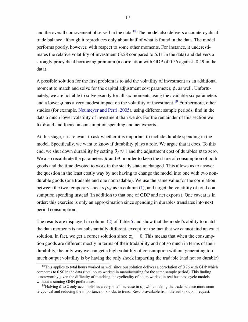
For the Czech Republic one can argue its integration in the European Union and its overallgreater integration into international capital markets made it less sensitive to external shocksand borrowing constraints. As for Taiwan Province of China, a possible explanation is thatits consumers seldom face binding borrowing constraints because of a high saving rate. InFigure 1 we plot the relative volatility of consumption against the average saving rate for the1960-1995 period for all countries in our sample.6 Although we do not want to imply any sortof causation, at this stage, there clearly is a negative relationship. This is an issue we explore
5For Israel and using data after 1995, for which reliability is higher, volatilities of consumption and invest-ment are lower than what is found using the entire sample. Regardless of the sample used for this country,results do not change qualitatively.
6Data is from the World Bank’s World Saving Database.
9
more below, when we deal with the calibration and simulation of a model of a small openeconomy with nondurables and durables, with and without financial frictions.
Table 2 shows the same variability within emerging market economies, now in terms of thecorrelation of the trade balance with output. While developed economies show uniformlymildly countercyclical trade balances (in line with the averages of -0.17 and -0.25 for OECDcountries reported by Aguiar and Gopinath, 2007 and Engel and Wang, 2011, respectively),emerging economies display results which go from mildly procyclical (Taiwan Province ofChina at 0.25) to strongly countercyclical net exports (Mexico at -0.82). In fact, the averagecorrelation of the trade balance with GDP is, in our sample, only -0.20. These results, how-ever, suffer from a small sample bias as they refer to a group of only a few emerging econo-mies, somewhat biased towards the most developed countries of that population. With a largersample for emerging economies at hand (but for which data on nondurables and durables ismissing), Aguiar and Gopinath find the average correlation between net exports and output tobe -0.51.
III. THE MODEL
The model we use here is a two-sector neoclassical growth model similar to the one in Aguiarand Gopinath (2007). In our small open economy, however, there are two types of consump-tion goods: durables and nondurables. The nondurable good is assumed to be non-tradablewhile the durable good is tradable across borders.7 This assumption is supported by the workof Engel and Wang (2011) who find that for the average OECD country, the share of durablesin imports and exports (excluding raw materials and energy) is 69 percent and 65 percent,respectively. For Mexico, these shares increase to 74 percent and 78 percent. So, althoughdurables represent a smaller fraction of total expenditure than nondurables, they account formost of the trade in goods.
We assume that markets are incomplete since individuals have only access to one financialasset, a risk-free bond which pays interest in units of the durable good. Output in each sectoris produced with labor and sector-specific capital. Durables can be used either for consump-tion or for capital accumulation. Nondurables can be used for consumption or as intermedi-ate inputs for the production of durables. The economy is subject to two temporary sectoral
7The assumption that nondurable goods are not traded across countries is needed to avoid an overdetermina-tion arising from the small country assumption for the bond market and factor price equalization across sectors.See Appendix A.3 for a more detailed argument.
10
aggregate TFP shocks and one aggregate shock to trend. The technology in the nondurablegood sector takes the following Cobb-Douglas form:
Yn,t = ezn,t Kαnn,t (ΓtLn,t)
1−αn ≡ Fn(Kn,t ,Ln,t ,zn,t ,Γt). (1)
For the durable good sector we assume a production function that combines a nondurableintermediate input in fixed proportions with capital and labor. This assumption of zero elas-ticity of substitution between the intermediate input and the value added component (whichdepends on capital and labor) is common in static general equilibrium models and seemsto be appropriate for a dynamic setting as well.8 The value-added component for durablesdepends on capital and labor combined as in a Cobb-Douglas production function. The tech-nology for the production of durables is
Yd,t = min
ezd,t Kαdd,t (ΓtLd,t)
1−αd︸ ︷︷ ︸≡Fd(Kd,t ,Ld,t ,zd,t ,Γt)
;Mn,t
Ω
, (2)
where Mn,t is the nondurable intermediate input used in the production of the durable goodand Ω is the number of units of the intermediate input needed to produce one unit of thedurable good (see Kehoe and Kehoe, 1994). The presence of intermediate goods acknowl-edges the important inter-sectoral links that characterize modern industrial economies. More-over, studies show that explicitly accounting for such relations in a model improves its abilityto reproduce some business cycle regularities; in particular, the comovement in output amongsectors (Hornstein and Praschnik, 1997). In (1) and (2), Γt is the common trend and Ki,t andLi,t denote capital and labor inputs, αi ∈ (0,1) represents the capital’s share of output, and zi,t
is the temporary stochastic productivity process in sector i, for i ∈ n,d. As in Aguiar andGopinath (2007), Γt = Γt−1egt , where gt is the (stationary) shock to trend. It is assumed thateach shock follows an AR(1) process such that
zn,t = ρnzn,t−1 + εn,t , (3)
zd,t = ρdzd,t−1 + εd,t , (4)
gt = (1−ρg) ln µg +ρggt−1 + εg,t , (5)
where εg,t is i.i.d N(0,σ2g ) and εn,t ,εd,t is an i.i.d. bivariate random variable N(0,ΣZ). The
contemporaneous covariance matrix of the shocks to the sectoral productivity processes, ΣZ ,
8 Using a dynamic general equilibrium model at quarterly frequency, Kouparitsas (1998) estimates the elas-ticity of substitution between these two components at 0.1, which is very close to the Leontief case.

11
is given by
ΣZ =
[σ2
n ρndσnσd
ρndσnσd σ2d
], (6)
where ρnd 6= 0 allows for contemporaneous correlation between the productivity processes.This is needed to generate comovement between sectoral outputs (Baxter, 1996) as we willshow in the next section. The assumption that the nondurable goods and the durable goodssectors share a common shock to trend is justified and is not overly restrictive.9 For instance,Galí (1993) models the changes in consumption of nondurables and durables as ARMA pro-cesses using the same assumption. Moreover, shocks to trend are often associated with clearlydefined changes in government policy (Aguiar and Gopinath, 2007) and are therefore expectedto affect all the sectors.
We assume that labor can be freely allocated between these two sectors so that in each period,
Lt = Ln,t +Ld,t . (7)
The representative agent’s expected lifetime utility is
E0
∞
∑t=0
βtU(Ct ,1−Lt), (8)
where Ct = C(Nt ,Dt) is a total consumption bundle which depends on both the current con-sumption of nondurable goods Nt and the stock of durable goods Dt .
We assume a constant elasticity of substitution between durables and nondurables, constantrelative risk aversion, and a Cobb-Douglas specification for the aggregate consumption bundleand leisure. The period utility function takes the form
U(Ct ,1−Lt) =
(Cθ
t (1−Lt)1−θ)1−σ
1−σ, where (9)
Ct ≡(
µN−γ
t +(1−µ)D−γ
t
)− 1γ
, (10)
and 11+γ
is the elasticity of substitution between durables and nondurables, µ is the utilityshare of nondurables, θ is the utility share of consumption, and σ is the coefficient of relativerisk aversion.
9In fact, all that is required, with respect to this, in order for the problem to have an interior solution is torestrict the trends to have the same long run mean growth.
12
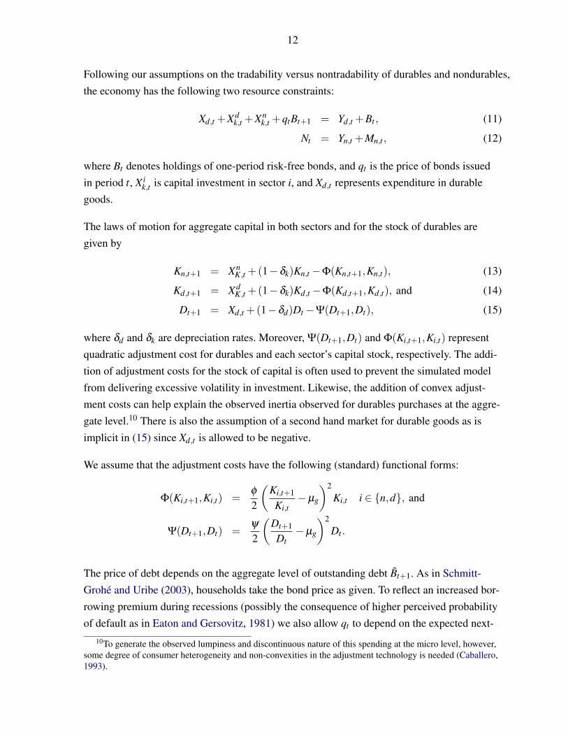
Following our assumptions on the tradability versus nontradability of durables and nondurables,the economy has the following two resource constraints:
Xd,t +Xdk,t +Xn
k,t +qtBt+1 = Yd,t +Bt , (11)
Nt = Yn,t +Mn,t , (12)
where Bt denotes holdings of one-period risk-free bonds, and qt is the price of bonds issuedin period t, X i
k,t is capital investment in sector i, and Xd,t represents expenditure in durablegoods.
The laws of motion for aggregate capital in both sectors and for the stock of durables aregiven by
Kn,t+1 = XnK,t +(1−δk)Kn,t−Φ(Kn,t+1,Kn,t), (13)
Kd,t+1 = XdK,t +(1−δk)Kd,t−Φ(Kd,t+1,Kd,t), and (14)
Dt+1 = Xd,t +(1−δd)Dt−Ψ(Dt+1,Dt), (15)
where δd and δk are depreciation rates. Moreover, Ψ(Dt+1,Dt) and Φ(Ki,t+1,Ki,t) representquadratic adjustment cost for durables and each sector’s capital stock, respectively. The addi-tion of adjustment costs for the stock of capital is often used to prevent the simulated modelfrom delivering excessive volatility in investment. Likewise, the addition of convex adjust-ment costs can help explain the observed inertia observed for durables purchases at the aggre-gate level.10 There is also the assumption of a second hand market for durable goods as isimplicit in (15) since Xd,t is allowed to be negative.
We assume that the adjustment costs have the following (standard) functional forms:
Φ(Ki,t+1,Ki,t) =φ
2
(Ki,t+1
Ki,t−µg
)2
Ki,t i ∈ n,d, and
Ψ(Dt+1,Dt) =ψ
2
(Dt+1
Dt−µg
)2
Dt .
The price of debt depends on the aggregate level of outstanding debt Bt+1. As in Schmitt-Grohé and Uribe (2003), households take the bond price as given. To reflect an increased bor-rowing premium during recessions (possibly the consequence of higher perceived probabilityof default as in Eaton and Gersovitz, 1981) we also allow qt to depend on the expected next-
10To generate the observed lumpiness and discontinuous nature of this spending at the micro level, however,some degree of consumer heterogeneity and non-convexities in the adjustment technology is needed (Caballero,1993).
13
period output level. This way,
qt =1
1+ r∗+χ
[exp( Bt+1
Γt− B)−1]+η
(Et
Yt+1Γt− Y) , (16)
where B and Y are the steady-sate levels of the detrended counterpart of the stock of bondsand total output. The countercyclical borrowing premia typically observed in emerging econ-omies should imply an η which is negative and much smaller for that type of economy thanfor developed economies. The borrowing premium implicit in (16) can be seen as a reducedform of several underlying mechanisms that potentially could generate a strongly countercy-clical real interest rate (see Neumeyer and Perri, 2005, for instance).
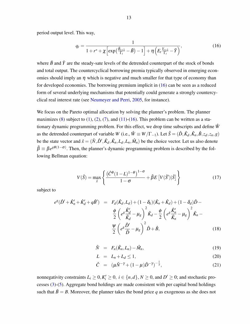
We focus on the Pareto optimal allocation by solving the planner’s problem. The plannermaximizes (8) subject to (1), (2), (7), and (11)-(16). This problem can be written as a sta-tionary dynamic programming problem. For this effect, we drop time subscripts and define W
as the detrended counterpart of variable W (i.e., W ≡W/Γ−1). Let S = (D, Kd, Kn, B,zd,zn,g)
be the state vector and x = (N, D′, Kd, Kn,Ld,Ln,Mn) be the choice vector. Let us also denoteβ ≡ βegθ(1−σ). Then, the planner’s dynamic programming problem is described by the fol-lowing Bellman equation:
V (S) = maxx
(Cθ (1−L)1−θ
)1−σ
1−σ+ βE
[V (S′)|S
](17)
subject to
eg(D′+ K′n + K′d +qB′) = Fd(Kd,Ld)+(1−δk)(Kn + Kd)+(1−δd)D−
φ
2
(eg K′d
Kd−µg
)2
Kd−φ
2
(eg K′n
Kn−µg
)2
Kn−
ψ
2
(eg D′
D−µg
)2
D+ B, (18)
N = Fn(Kn,Ln)− Mn, (19)
L = Ln +Ld ≤ 1, (20)
C = (µN−γ +(1−µ)D−γ)−1γ , (21)
nonnegativity constraints Li ≥ 0,K′i ≥ 0, i ∈ n,d, N ≥ 0, and D′ ≥ 0; and stochastic pro-cesses (3)-(5). Aggregate bond holdings are made consistent with per capital bond holdingssuch that B = B. Moreover, the planner takes the bond price q as exogenous as she does not
14
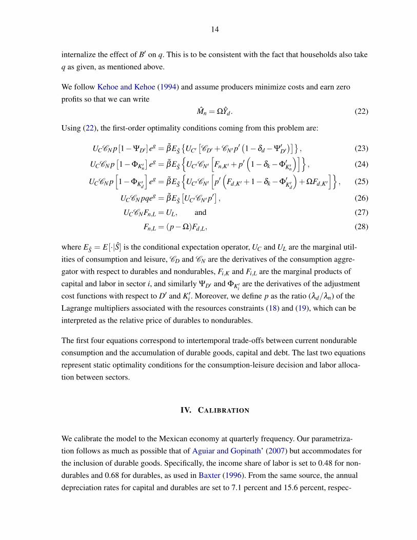
internalize the effect of B′ on q. This is to be consistent with the fact that households also takeq as given, as mentioned above.
We follow Kehoe and Kehoe (1994) and assume producers minimize costs and earn zeroprofits so that we can write
Mn = ΩYd. (22)
Using (22), the first-order optimality conditions coming from this problem are:
UCCN p [1−ΨD′]eg = βES
UC′[CD′+CN′ p
′ (1−δd−Ψ′D′)]
, (23)
UCCN p[1−ΦK′n
]eg = βES
UC′CN′
[Fn,K′+ p′
(1−δk−Φ
′K′n
)], (24)
UCCN p[1−ΦK′d
]eg = βES
UC′CN′
[p′(
Fd,K′+1−δk−Φ′K′d
)+ΩFd,K′
], (25)
UCCN pqeg = βES
[UC′CN′ p
′] , (26)
UCCNFn,L =UL, and (27)
Fn,L = (p−Ω)Fd,L, (28)
where ES = E[·|S] is the conditional expectation operator, UC and UL are the marginal util-ities of consumption and leisure, CD and CN are the derivatives of the consumption aggre-gator with respect to durables and nondurables, Fi,K and Fi,L are the marginal products ofcapital and labor in sector i, and similarly ΨD′ and ΦK′i
are the derivatives of the adjustmentcost functions with respect to D′ and K′i . Moreover, we define p as the ratio (λd/λn) of theLagrange multipliers associated with the resources constraints (18) and (19), which can beinterpreted as the relative price of durables to nondurables.
The first four equations correspond to intertemporal trade-offs between current nondurableconsumption and the accumulation of durable goods, capital and debt. The last two equationsrepresent static optimality conditions for the consumption-leisure decision and labor alloca-tion between sectors.
IV. CALIBRATION
We calibrate the model to the Mexican economy at quarterly frequency. Our parametriza-tion follows as much as possible that of Aguiar and Gopinath’ (2007) but accommodates forthe inclusion of durable goods. Specifically, the income share of labor is set to 0.48 for non-durables and 0.68 for durables, as used in Baxter (1996). From the same source, the annualdepreciation rates for capital and durables are set to 7.1 percent and 15.6 percent, respec-
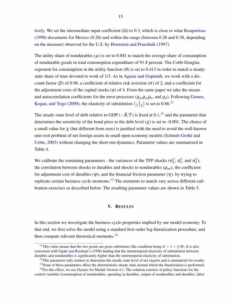
15
tively. We set the intermediate input coefficient (Ω) to 0.3, which is close to what Kouparitsas(1998) documents for Mexico (0.28) and within the range (between 0.26 and 0.38, dependingon the measure) observed for the U.S. by Hornstein and Praschnik (1997).
The utility share of nondurables (µ) is set to 0.881 to match the average share of consumptionof nondurable goods in total consumption expenditure of 91.8 percent. The Cobb-Douglasexponent for consumption in the utility function (θ ) is set to 0.413 in order to match a steady-state share of time devoted to work of 1/3. As in Aguiar and Gopinath, we work with a dis-count factor (β ) of 0.98, a coefficient of relative risk aversion (σ ) of 2, and a coefficient forthe adjustment costs of the capital stocks (φ ) of 4. From the same paper we take the meansand autocorrelation coefficients for the error processes (µg,ρg,ρn, and ρd). Following Gomes,Kogan, and Yogo (2009), the elasticity of substitution
( 11+γ
)is set to 0.86.11
The steady-state level of debt relative to GDP (−B/Y ) is fixed at 0.1,12 and the parameter thatdetermines the sensitivity of the bond price to the debt level (χ) is set to -0.001. The choice ofa small value for χ (but different from zero) is justified with the need to avoid the well-knownunit root problem of net foreign assets in small open economy models (Schmitt-Grohé andUribe, 2003) without changing the short-run dynamics. Parameter values are summarized inTable 4.
We calibrate the remaining parameters - the variances of the TFP shocks (σ2g , σ2
n , and σ2d ),
the correlation between shocks to durables and shocks to nondurables (ρnd), the coefficientfor adjustment cost of durables (ψ), and the financial friction parameter (η), by trying toreplicate certain business cycle moments.13 The moments to match vary across different cali-bration exercises as described below. The resulting parameter values are shown in Table 5.
V. RESULTS
In this section we investigate the business cycle properties implied by our model economy. Tothat end, we first solve the model using a standard first-order log-linearization procedure, andthen compute relevant theoretical moments.14
11This value means that the two goods are gross substitutes (the condition being σ > 1+ γ/θ ). It is alsoconsistent with Ogaki and Reinhart’s (1998) finding that the intratemporal elasticity of substitution betweendurables and nondurables is significantly higher than the intertemporal elasticity of substitution.
12This parameter only matters to determine the steady-state level of net exports and is immaterial for results.13None of these parameters affect the deterministic steady state around which the linearization is performed.14For this effect, we use Dynare for Matlab Version 4.1. The solution consists of policy functions for the
control variables (consumption of nondurables, spending in durables, output of nondurables and durables, labor

16
Table 5 presents business cycle moments for GDP (total value added), sectoral output (indus-trial production), total consumption expenditure, nondurable consumption, spending in durables,the net exports-output ratio, investment, and the borrowing premium. Moreover, we showa measure of the quality of fit of the simulation (the sum of the square deviations of all thesimulated moments relative to the sample moments, normalized by the total variation of allthe sample moments) and three measures of the contribution of the permanent shock to non-durables (wn), to durables (wd), and to the variance of output.15 Each column (1)-(5) displaysthe results for a different calibration exercise as we now explain.
A. No Financial Frictions Case
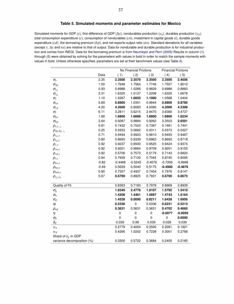
Our first exercise is to solve for the variances of the TFP shocks as well as ψ and ρnd to matchthe volatilities of GDP, consumption of nondurables, durables expenditure, and the net exports-GDP ratio as well as the correlation between the two sectoral outputs.16 Here, we stay asclose as possible to Aguiar and Gopinath’s (2007) model. In particular, we set the borrowingpremium parameter η = 0. We call this scenario the no financial frictions case.17 We obtainσg = 1.8340, σn = 1.4209, σd = 1.4528, ψ = 0.5336 and ρnd = 0.3631, as shown in col-umn (1) of Table 5, and are able to exactly match the targeted moments (in bold). The esti-mates of the random walk component of the sectoral Solow residuals are substantially smallerthan what Aguiar and Gopinath find for Mexico (0.28 and 0.43 for nondurables and durables,respectively against 0.96). As a result, the permanent shock accounts for about 32 percent ofGDP volatility.
As an initial conclusion based on this first simulation results, we find that our framework doesa good job at capturing the high volatility of consumption of nondurables and spending indurables. It does reasonably well in mimicking the volatility of total consumption spending
for durables and nondurables, and the relative price of durables) and laws of motion for the endogenous states(capital stocks, durables stock, and bond holdings) as a function of the states and forcing variables (shocks todurables and nondurables and shock to trend).
15The first two measures are the random walk components for the nondurable and durable sectors calculatedas in equation (14) of Aguiar and Gopinath’s (2007) paper and the third comes from a variance decomposition ofGDP.
16We use quarterly data for industrial production in the sectors of consumer durables and nondurables. Thisdata is also from INEGI and covers the same sample period as all other data used for Mexico.
17We are aware that the fact that the bond price is sensitive to the aggregate debt level is in itself a financialfriction. As mentioned before, the size of that friction (χ) is set to such a small value that it does not signifi-cantly affect the short run dynamics of the simulated economy.
17
and the overall comovement observed in the data.18 The model also delivers a countercyclicaltrade balance although it reproduces only about half of what is found in the data. The modelperforms poorly, however, with respect to some other moments. For instance, it underesti-mates the relative volatility of investment (3.28 compared to 6.11 in the data) and delivers astrongly procyclical borrowing premium (a correlation with GDP of 0.56 against -0.49 in thedata).
A possible solution for the first problem is to add the volatility of investment as an additionalmoment to match and solve for the capital adjustment cost parameter, φ , as well. Unfortu-nately, we are not able to solve exactly for all six moments using the available six parametersand a lower φ has a very modest impact on the volatility of investment.19 Furthermore, otherstudies (for example, Neumeyer and Perri, 2005), using different sample periods, find in thedata a much lower volatility of investment than we do. For the remainder of this section wefix φ at 4 and focus on consumption spending and net exports.
At this stage, it is relevant to ask whether it is important to include durable spending in themodel. Specifically, we want to know if durability plays a role. We argue that it does. To thisend, we shut down durability by setting δd ≈ 1 and the adjustment cost of durables ψ to zero.We also recalibrate the parameters µ and θ in order to keep the share of consumption of bothgoods and the time devoted to work in the steady state unchanged. This allows us to answerthe question in the least costly way by not having to change the model into one with two non-durable goods (one tradable and one nontradable). We use the same value for the correlationbetween the two temporary shocks ρnd as in column (1), and target the volatility of total con-sumption spending instead (in addition to that one of GDP and net exports). One caveat is inorder: this exercise is only an approximation since spending in durables translates into nextperiod consumption.
The results are displayed in column (2) of Table 5 and show that the model’s ability to matchthe data moments is not substantially different, except for the fact that we cannot find an exactsolution. In fact, we get a corner solution since σd = 0. This means that when the consump-tion goods are different mostly in terms of their tradability and not so much in terms of theirdurability, the only way we can get a high volatility of consumption without generating toomuch output volatility is by having the only shock impacting the tradable (and not so durable)
18This applies to total hours worked as well since our solution delivers a correlation of 0.76 with GDP whichcompares to 0.90 in the data (total hours worked in manufacturing for the same sample period). This findingis noteworthy given the difficulty of matching the cyclicality of hours worked in real business cycle modelswithout assuming GHH preferences.
19Halving φ to 2 only accomplishes a very small increase in σi, while making the trade balance more coun-tercyclical and reducing the importance of shocks to trend. Results available from the authors upon request.
18
good being of a permanent nature. This naturally increases the importance of shocks to trend,which now contribute with 57 percent of GDP volatility.
The exercise of column (2) incorporates two changes when compared to our first calibrationin column (1). First, we are shutting down durability. Second, we are targeting total consump-tion instead of disaggregated consumption. We argue that both changes increase the relevanceof shocks to trend. On the one hand, since we no longer target the (low) relative volatility ofnondurable consumption, we do not impose so much discipline on the shock process and par-ticularly on σg. To isolate this effect, we redo column (2) with δd at its benchmark value andψ at its calibrated value in column (1). We find that shocks to trend contribute with about 37percent of output variance (column 3), which is around 10 percent greater than in column (1).We attribute this increase to the fact that we are targeting the volatility of total consumptioninstead of the volatilities of each component of spending. On the other hand, with low dura-bility, “durable" expenditure does not respond nearly as much to shocks, and the only way togenerate high volatility of total consumption is by having a significantly larger σg.
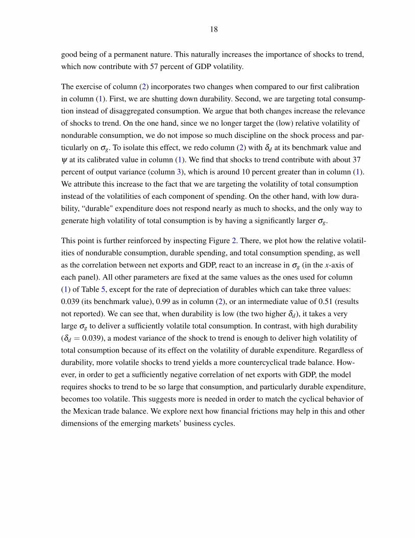
This point is further reinforced by inspecting Figure 2. There, we plot how the relative volatil-ities of nondurable consumption, durable spending, and total consumption spending, as wellas the correlation between net exports and GDP, react to an increase in σg (in the x-axis ofeach panel). All other parameters are fixed at the same values as the ones used for column(1) of Table 5, except for the rate of depreciation of durables which can take three values:0.039 (its benchmark value), 0.99 as in column (2), or an intermediate value of 0.51 (resultsnot reported). We can see that, when durability is low (the two higher δd), it takes a verylarge σg to deliver a sufficiently volatile total consumption. In contrast, with high durability(δd = 0.039), a modest variance of the shock to trend is enough to deliver high volatility oftotal consumption because of its effect on the volatility of durable expenditure. Regardless ofdurability, more volatile shocks to trend yields a more countercyclical trade balance. How-ever, in order to get a sufficiently negative correlation of net exports with GDP, the modelrequires shocks to trend to be so large that consumption, and particularly durable expenditure,becomes too volatile. This suggests more is needed in order to match the cyclical behavior ofthe Mexican trade balance. We explore next how financial frictions may help in this and otherdimensions of the emerging markets’ business cycles.
19
B. Financial Frictions Case
Two dimensions where the model thus far fares poorly are in capturing the volatility of theborrowing premium (which it grossly underestimates) and in mimicking its countercyclicalbehavior (in the first two simulations it comes very procyclical). Here we attempt to disciplinethe dynamics of the model in this dimension by introducing financial frictions.
One simple way to do this is to match the volatility of the borrowing premium by choosing anappropriate value for χ . This is what García-Cicco, Pancrazi, and Uribe (2010) do in a RBCmodel with financial frictions but no durables. They do not report, however, the simulatedmoments for the borrowing premium and focus on the autocorrelation of net exports.
An alternative way of introducing a financial friction is to have a non-zero income-elasticityof the borrowing premium, which is defined by the parameter η . A negative value for η impliesa countercyclical borrowing premium and is consistent with what Neumeyer and Perri (2005)call the induced country risk case. We choose this route instead of calibrating χ because,if we target the observed correlation of the borrowing premium with output, the latter mayintroduce a bias against shocks to trend. The reason for this bias is that a positive permanentshock causes agents to borrow more and increase their stock of debt which, given χ < 0,causes the borrowing premium to increase as well and, therefore, to be counterfactually pro-cyclical. Therefore, targeting the cyclical dynamics of the borrowing premium may diminishthe importance of shocks to trend.
In column (4), we present the results when we target the volatilities of GDP, nondurables con-sumption, expenditure in durables, the net exports-GDP ratio, and the borrowing premium aswell as the correlation between the two sectoral outputs by solving for σg, σn, σd , ψ , ρnd andη . What we do here is to extend the calibration exercise in column (1) by adding one param-eter (η) and one moment (ρbp,y). First, we should note that we are able to find an exact solu-tion and that there is a substantial improvement in the quality of fit of the model compared tocolumn (1). Second, we get an estimate for η of -0.0077, consistent with the induced country
risk hypothesis. Third, even though we were not explicitly targeting this moment, the correla-tion of net exports-GDP ratio with GDP (at -0.72) gets much closer to its sample counterpart.Fourth, the importance of the shocks to trend falls, accounting now for about 24 percent ofGDP variance.
The reason why a model with durables and financial frictions is able to deliver more coun-tercyclical net exports can be found in the interaction between the accumulation of durablesand the countercyclical borrowing premium. The financial friction introduced in our model,
20
which mimics an empirical fact, implies that interest rates are countercyclical and relativelymore volatile. As a consequence, during booms the economy can take advantage of cheapercredit by borrowing more to build capital and increase the stock of durables. Since durablesare mostly tradable (another empirical fact), part of the accumulation of durables (and capital)will resort to imports. As a consequence, net exports fall during economic expansions makingthe trade balance countercyclical.
This point is made clear when we compare the impulse-response functions generated by themodel with and without the financial friction, which we present in figures 3 through 5.20 InFigure 3, we show the response of our model economy to a permanent technology shock. It isclear that for all variables except the borrowing premium, the financial friction does not playa significant role when a permanent shock hits the economy. The main intuition why financialfrictions are not crucial in the case of a permanent shocks is that (transitory) changes in theborrowing premium do not affect durable spending because the wealth effect induced by theshock is much stronger than the intertemporal substitution effect coming from any change inthe interest rate.
In contrast, the financial friction does seem to generate very different dynamics when thereexists a temporary shock to nondurable’s TFP. As shown in Figure 4, the borrowing premiumfalls only in the presence of the friction. Therefore, with the financial friction, the interest-rate-sensitive durable spending and investment increase much more and net exports relative toGDP experience a larger drop. In the absence of the friction, durables’ accumulation respondsless to the shock, borrowing initially increases but eventually declines (standard result underthe permanent income hypothesis) and the net exports-GDP ratio drops less and increasesearlier.
By inspecting Figure 5, we observe that the financial friction does not seem to be nearly asimportant in the case of a temporary shock to durables’ production. The reason for this is thatdurables represent a relatively small fraction of total output. Therefore, this shock does notcause output to deviate as much from its steady state and, consequently, the borrowing pre-mium does not move as much either as in the case of a transitory nondurable shock.
To highlight the impact of financial frictions on key business cycle moments and show howthey interact with the relative importance of shocks to trend, we show in Figure 6 how therelative volatilities of consumption expenditure (nondurable, durable, and total), as well asthe correlation of the net exports-output ratio and GDP, respond to an increase in financial
20In these figures, we use the parameters values in column (4) of Table 5 unless otherwise indicated.
21
frictions (lower η in the x-axis of each panel) for three different values of σg. The remainingparameter values are the same as in column (1) of Table 5. We observe that as financial fric-tions increase, the correlation of net exports with GDP is much less sensitive to changes inthe magnitude of the shock to trend (relative to the magnitude of the temporary TFP shocks)and is basically determined by the size of the friction. The relative volatility of the shock totrend, in turn, helps pin down the volatilities of nondurable consumption and durable spend-ing because both expenditures vary with σg for any level of η .
C. Robustness
Uribe and Yue (2006) argue that other shocks to the interest rate, independent of income, aremore important to explain the movements of country interest rate premia. For this reasonwe modify (16) by adding an orthogonal shock to the borrowing premium, εb,21 with vari-ance σ2
b . We then try to match the volatility of the borrowing premium as well. In this case,according to the results presented in column (5), we are not able to exactly match the sevenmoments. The overall quality of fit, however, remains almost the same and the estimate for σb
is zero. In fact, the results column (5) can be seen as an overdetermined version of the esti-mation results presented in column (4). We interpret this result as evidence of the existenceof other types of financial frictions in emerging economies which need to be correlated withincome.
A more serious robustness concern relates to a possible bias against shocks to trend, in thepresence of financial frictions, built into our specification of the borrowing premium. In (16),the borrowing premium depends on the induced country risk term, η(EtYt+1/Γt − Y ). Witha negative η , the borrowing premium increases whenever output falls below trend. This hap-pens not only when we have negative temporary income shocks but also when we have a pos-itive permanent shock. This is clear in the impulse response of the borrowing premium to apermanent shock, which we plot in Figure 3. After such a shock, output initially grows belowtrend and the interest rate increases. This, in turn, makes the borrowing premium counterfac-tually procyclical. Therefore, in order to have a countercyclical borrowing premium, shocksto trend need to be small. The concern is, then, that the smaller role of shocks to trend mightbe a by-product of the way we specify the induced country risk term.
21Since (16) now becomes qt =1
1+r∗+χ
[exp( Bt+1
Γt−B)−1]+η
(Et
Yt+1Γt−Y
)+εb
, this new shock can also be inter-
preted as an orthogonal shock to the world interest rate.
22
For this reason, we rewrite the borrowing premium in order to make it explicitly dependent oneach of the three shocks to income. Therefore, we replace (16) with
qt =1
1+ r∗+χ
[exp( Bt+1
Γt− B)−1]+ηg(gt−µg)+ηnzn,t +ηdzd,t
.
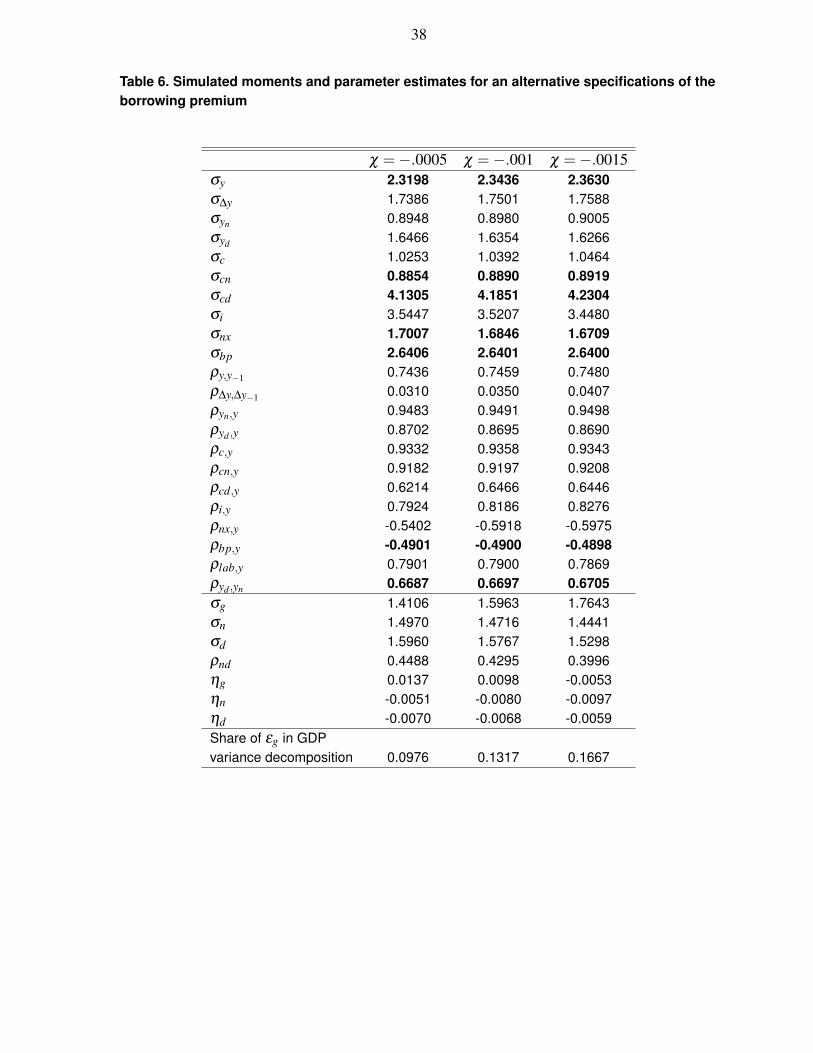
A priori we have no reason to expect the η parameters to be positive or negative. In fact, apositive ηg, for instance, can be capturing increased interest rates not because of improvedeconomic activity but because of increased borrowing following a permanent shock. We callthis the indebtness effect. This effect could, in principle, be captured by more debt-elasticinterest rates, i.e., by χ being more negative. For this reason, we solve the model for differ-ent values of χ: -0.0005, -0.001, and -0.0015. If the indebtness effect is at play, the estimatedηg parameter should decrease in value as χ becomes more negative.
Table 6 shows this conjecture to be correct.22 In particular, ηg is positive for small valuesof χ . Therefore, for the benchmark value of χ = −0.001, the bias introduced by our origi-nal specification of the borrowing premium is of second order since the positive associationbetween shocks to trend and the borrowing premium, implied by the term η(EtYt+1/Γt − Y )
in our original specification, is explained by the indebtedness effect. When comparing theresults of Table 6 to those of columns (4) and (5) in Table 5, we find that they are qualitativelythe same, except for the fact that the contribution of the permanent shock to the volatility ofGDP is even smaller. Furthermore, the original specification has the advantage of being moreparsimonious and actually delivering a better fit. We conclude, then, that our results are robustto this source of misspecification.
VI. CONCLUSIONS
This paper presents a small open economy neoclassical growth model with consumer durables,nondurable goods, shocks to the trend, and temporary sector-specific shocks. We calibrate themodel to the Mexican economy as representative of an emerging market. We find that finan-cial frictions in the form of a countercyclical country risk premium play an essential role inexplaining a few empirical facts that characterize cyclical fluctuations in developing econ-
22There, we try to match the same seven moments as in column (5) of Table (5) by solving the variancesof the three shocks to income, the correlation between the sector-specific shocks, and the three η parameters.In order to have an exactly identified problem, we need to fix one previously free parameter. We choose to setψ = 0.6, which is within the range of values we get from the baseline specification.
23
omies. Namely, financial frictions are important to explain a strongly countercyclical tradebalance, and a countercyclical and very volatile borrowing premium.
Our result is in line with Neumeyer and Perri’s (2005) finding. The main difference, however,is that we do not need to introduce any friction on the firm side and exploit only the natureof durables accumulation to achieve the desired magnification effect on spending. This resultis also consistent with and reinforces that of García-Cicco, Pancrazi, and Uribe (2010). Ourpaper, however, stresses the interaction of durables expenditure (not considered by García-Cicco, Pancrazi, and Uribe) with financial frictions.
Our results indicate that shocks to trend are somewhat relevant in explaining output and con-sumption fluctuations in developing countries. These shocks, however, do not appear to be themain source of economic fluctuation in emerging economies. The simulations seem to show,though, that some additional work needs to be done in terms of matching some moments,namely the volatility of investment.
A natural extension to this paper is to consider other types of shocks. For instance, exogenousshocks to the borrowing premium when durables and nondurables are present should be con-sidered as a complementary explanation, as the work by Uribe and Yue (2006), Fernández-Villaverde and others (2009) and Gruss and Mertens (2009) seems to suggest. We find thatorthogonal shocks to the interest rate do not seem to be important to match business cyclemoments in emerging markets. We feel, however, that other types of shocks to the borrowingpremium may play a role and that more work is needed.
Another possibility for future research should consider exploring the importance of othertypes of financial frictions and external shocks in explaining the properties of business cyclesin emerging markets. For example, we can think of shocks to external wealth which inter-act with domestic spending in a variety of ways. One straightforward channel is to see howthese shocks trigger a portfolio rebalancing and cause foreign investors to sell out assets inemerging markets. This in turn depresses domestic asset prices and lowers permanent incomethereby affecting consumption of both durables and nondurables.
An alternative driving force to be considered, under the presence of durable goods, comesfrom shocks to the terms of trade. Many emerging economies are fundamentally producersof commodities and the prices of many commodities, by their nature, are subject to regimeswitching. Consider, for example, an increase in the variance of the terms of trade. As exter-nal income becomes more volatile, default incentives get smaller and, as a consequence, for-eign debt conditions endogenously improve. On the one hand, this allows for smoother con-
24
sumption of nondurables, but on the other hand, the purchase of durables may react as house-holds want to take advance of better borrowing conditions. As a consequence, this type ofshocks may imply a high volatility in the purchase of durable goods and a relatively smallvolatility of consumption of non-durables with respect to income volatility. This extensionwould also be important in adding micro-foundations to the borrowing premium within abusiness cycle model, an important avenue for future research.
25
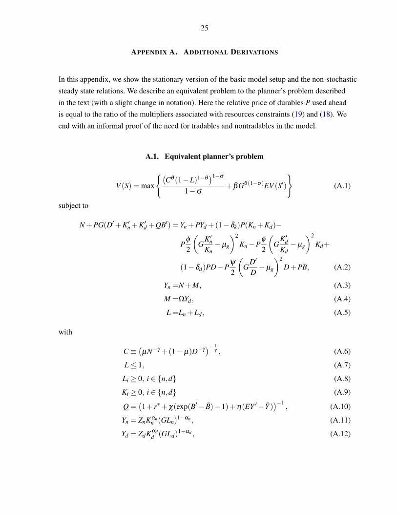
APPENDIX A. ADDITIONAL DERIVATIONS
In this appendix, we show the stationary version of the basic model setup and the non-stochasticsteady state relations. We describe an equivalent problem to the planner’s problem describedin the text (with a slight change in notation). Here the relative price of durables P used aheadis equal to the ratio of the multipliers associated with resources constraints (19) and (18). Weend with an informal proof of the need for tradables and nontradables in the model.
A.1. Equivalent planner’s problem
V (S) = max
(Cθ (1−L)1−θ
)1−σ
1−σ+βGθ(1−σ)EV (S′)
(A.1)
subject to
N +PG(D′+K′n +K′d +QB′) = Yn +PYd +(1−δk)P(Kn +Kd)−
Pφ
2
(G
K′nKn−µg
)2
Kn−Pφ
2
(G
K′dKd−µg
)2
Kd+
(1−δd)PD−Pψ
2
(G
D′
D−µg
)2
D+PB, (A.2)
Yn =N +M, (A.3)
M =ΩYd, (A.4)
L =Ln +Ld, (A.5)
with
C ≡(µN−γ +(1−µ)D−γ
)− 1γ , (A.6)
L≤ 1, (A.7)
Li ≥ 0, i ∈ n,d (A.8)
Ki ≥ 0, i ∈ n,d (A.9)
Q =(1+ r∗+χ(exp(B′− B)−1)+η(EY ′− Y )
)−1, (A.10)
Yn = ZnKαnn (GLn)
1−αn, (A.11)
Yd = ZdKαdd (GLd)
1−αd , (A.12)
26
lnG′ = (1−ρg) ln µg +ρg lnG+ εg, (A.13)
lnZ′n = ρn lnZn + εn, (A.14)
lnZ′d = ρd lnZd + εd. (A.15)
The exogenous variables in this problem are the shocks to Zn, Zd , and G. The endogenousstates are Kn, Kd , D, and B. The controls are P, N, Ln, and Ld .
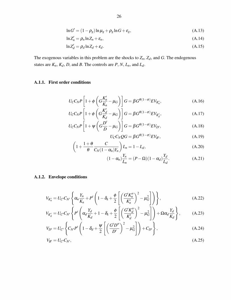
A.1.1. First order conditions
UCCNP[
1+φ
(G
K′nKn−µG
)]G = βGθ(1−σ)EVK′n, (A.16)
UCCNP[
1+φ
(G
K′dKd−µG
)]G = βGθ(1−σ)EVK′d
, (A.17)
UCCNP[
1+ψ
(G
D′
D−µG
)]G = βGθ(1−σ)EVD′, (A.18)
UCCNQG = βGθ(1−σ)EVB′, (A.19)(1+
1+θ
θ
CCN(1−αn)Yn
)Ln = 1−Ld, (A.20)
(1−αn)Yn
Ln= (P−Ω)(1−αd)
Yd
Ld. (A.21)
A.1.2. Envelope conditions
VK′n =UC′CN′
αn
Yn
Kn+P′
(1−δk +
φ
2
[(G′K′′n
K′n
)2
−µ2G
]), (A.22)
VK′d=UC′CN′
P′(
αdYd
Kd+1−δk +
φ
2
[(G′K′′d
K′d
)2
−µ2G
])+Ωαd
Yd
Kd
, (A.23)
VD′ =UC′
CN′P
′
(1−δd +
ψ
2
[(G′D′′
D′
)2
−µ2G
])+CD′
, (A.24)
VB′ =UC′CN′, (A.25)
27
where
UC = θCθ(1−σ)−1(1−L)(1−θ)(1−σ), (A.26)
CN = µN−γ−1 (µN−γ +(1−µ)D−γ
)− 1γ−1
, and (A.27)
CD = (1−µ)D−γ−1 (µN−γ +(1−µ)D−γ
)− 1γ−1
. (A.28)
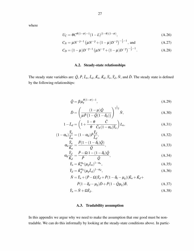
A.2. Steady-state relationships
The steady state variables are: Q, P, Ln, Ld , Kn, Kd , Yn, Yd , N, and D. The steady state is definedby the following relationships:
Q = β µθ(1−σ)−1g , (A.29)
D =
((1−µ)Q
µP(1− Q(1−δd)
)) 11+γ
N, (A.30)
1− Ld =
(1+
1−θ
θ
CCN(1−αn)Yn
)Ln, (A.31)
(1−αn)Yn
Ln= (1−αd)P
Yd
Ld, (A.32)
αnYn
Kn=
P(1− (1−δk)Q)
Q, (A.33)
αdYd
Kd=
P−Ω
P1− (1−δk)Q
Q, (A.34)
Yn = Kαnn (µgLn)
1−αn , (A.35)
Yd = Kαdd (µgLd)
1−αd , (A.36)
N = Yn +(P−Ω)Yd + P(1−δk−µg)(Kn + Kd+
P(1−δd−µg)D+ P(1− Qµg)B, (A.37)
Yn = N +ΩYd. (A.38)
A.3. Tradability assumption
In this appendix we argue why we need to make the assumption that one good must be non-tradable. We can do this informally by looking at the steady-state conditions above. In partic-
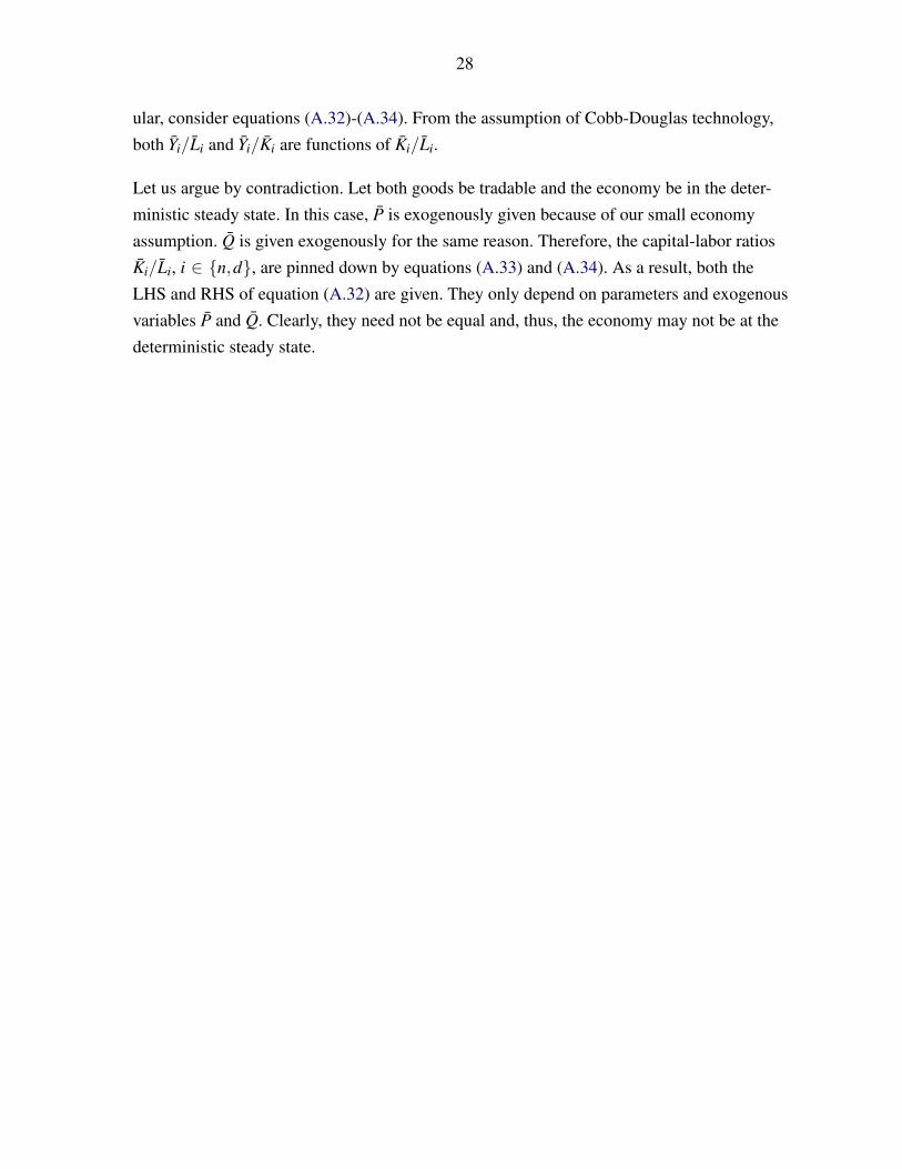
28
ular, consider equations (A.32)-(A.34). From the assumption of Cobb-Douglas technology,both Yi/Li and Yi/Ki are functions of Ki/Li.
Let us argue by contradiction. Let both goods be tradable and the economy be in the deter-ministic steady state. In this case, P is exogenously given because of our small economyassumption. Q is given exogenously for the same reason. Therefore, the capital-labor ratiosKi/Li, i ∈ n,d, are pinned down by equations (A.33) and (A.34). As a result, both theLHS and RHS of equation (A.32) are given. They only depend on parameters and exogenousvariables P and Q. Clearly, they need not be equal and, thus, the economy may not be at thedeterministic steady state.
29
REFERENCES
Aguiar, Mark, and Gita Gopinath, 2007, “Emerging Market Business Cycles: The Cycle is theTrend,” Journal of Political Economy, Vol. 115, No. 1, pp. 69–102.
Baxter, Marianne, 1996, “Are Consumer Durables Important for Business Cycles?” Review ofEconomics and Statistics, Vol. 78, No. 1, pp. 147–155.
Boz, Emine, Christian Daude, and Ceyhun B. Durdu, 2008, “Emerging Market BusinessCycles Revisited: Learning About the Trend,” International Finance Discussion Paper 927,Federal Reserve Board.
Caballero, Ricardo J., 1993, “Durable Goods: An Explanation for Their Slow Adjustment,”Journal of Political Economy, Vol. 101, No. 2, pp. 351–384.
De Gregorio, Jose, Pablo E. Guidotti, and Carlos A. Vegh, 1998, “Inflation Stabilisation andthe Consumption of Durable Goods,” Economic Journal, Vol. 108, No. 446, pp. 105–131.
De Resende, Carlos, 2006, “Endogenous Borrowing Constraints and Consumption Volatilityin a Small Open Economy,” Working Paper 06-37, Bank of Canada.
Eaton, Jonathan, and Mark Gersovitz, 1981, “Debt with Potential Repudiation: Theoreticaland Empirical Analysis,” Review of Economic Studies, Vol. 48, No. 2, pp. 289–309.
Engel, Charles, and Jian Wang, 2011, “International Trade in Durable Goods: UnderstandingVolatility, Cyclicality, and Elasticities,” Journal of International Economics, Vol. 83, No. 1,pp. 37–52.
Fernández-Villaverde, Jesús, Pablo A. Guerrón-Quintana, Juan Rubio-Ramírez, and MartínUribe, 2009, “Risk Matters: The Real Effects of Volatility Shocks,” Working Paper 14875,National Bureau of Economic Research.
Galí, Jordi, 1993, “Variability of Durable and Nondurable Consumption: Evidence for SixO.E.C.D. Countries,” Review of Economics and Statistics, Vol. 75, No. 3, pp. 418–428.
García-Cicco, Javier, Roberto Pancrazi, and Martín Uribe, 2010, “Real Business Cycles inEmerging Countries?” American Economic Review, Vol. 100, No. 5, pp. 2510–31.
Gomes, João F., Leonid Kogan, and Motohiro Yogo, 2009, “Durability of Output andExpected Stock Returns,” Journal of Political Economy, Vol. 117, No. 5, pp. 941–986.
Gruss, Bertrand, and Karel Mertens, 2009, “Regime Switching Interest Rates and Fluctua-tions in Emerging Markets,” Economics Working Paper ECO2009/22, European UniversityInstitute.
Hornstein, Andreas, and Jack Praschnik, 1997, “Intermediate Inputs and Sectoral Comove-ment in the Business Cycle,” Journal of Monetary Economics, Vol. 40, No. 3, pp. 573–595.
30
Kehoe, Patrick J., and Timothy J. Kehoe, 1994, “A Primer on Static Applied General Equi-librium Models,” Federal Reserve Bank of Minneapolis Quarterly Review, Vol. 18, No. 1, pp.2–16.
Kouparitsas, Michael, 1998, “Dynamic Trade Liberalization Analysis: Steady State, Tran-sitional and Inter-Industry Effects,” Working Paper WP-98-15, Federal Reserve Bank ofChicago.
Mendoza, Enrique G., 1991, “Real Business Cycles in a Small Open Economy,” AmericanEconomic Review, Vol. 81, No. 4, pp. 797–818.
Neumeyer, Pablo A., and Fabrizio Perri, 2005, “Business Cycles in Emerging Economies:The Role of Interest Rates,” Journal of Monetary Economics, Vol. 52, No. 2, pp. 345–380.
Ogaki, Masao, and Carmen M. Reinhart, 1998, “Measuring Intertemporal Substitution: TheRole of Durable Goods,” Journal of Political Economy, Vol. 106, No. 5, pp. 1078–1098.
Restrepo-Echevarria, Paulina, 2008, “Business Cycles in Developing vs. Developed Coun-tries: The Importance of the Informal Economy,” Working paper, UCLA.
Rosenzweig, Mark R., and Kenneth I. Wolpin, 1993, “Credit Market Constraints, Consump-tion Smoothing, and the Accumulation of Durable Production Assets in Low-Income Coun-tries: Investments in Bullocks in India,” Journal of Political Economy, Vol. 101, No. 2, pp.223–244.
Schmitt-Grohé, Stephanie, and Martín Uribe, 2003, “Closing Small Open Economy Models,”Journal of International Economics, Vol. 61, No. 1, pp. 163–185.
Uribe, Martín, and Vivian Z. Yue, 2006, “Country Spreads and Emerging Countries: WhoDrives Whom?” Journal of International Economics, Vol. 69, No. 1, pp. 6–36.
31
Figure 1. Relative Volatility of Consumption and Saving Rates Across Countries
Figure 2. Effect of Shocks to Trend on Key Moments
32
Figure 3. Impulse-Response Functions for a Permanent Shock
The dotted line refers to the trend of the variable under consideration.
Figure 4. Impulse-Response Functions for a Shock to Nondurables

33
Figure 5. Impulse-Response Functions for a Shock to Durables
Figure 6. Effect of Financial Frictions on Key Moments
34
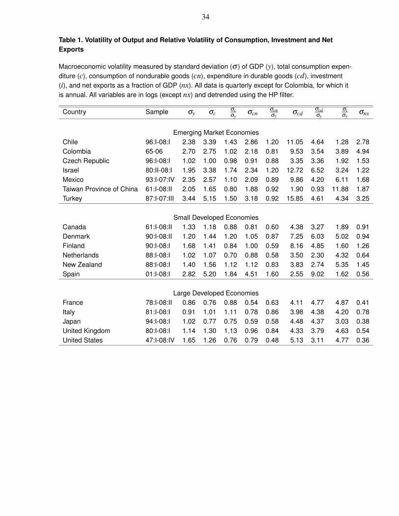
Table 1. Volatility of Output and Relative Volatility of Consumption, Investment and NetExports
Macroeconomic volatility measured by standard deviation (σ ) of GDP (y), total consumption expen-diture (c), consumption of nondurable goods (cn), expenditure in durable goods (cd), investment(i), and net exports as a fraction of GDP (nx). All data is quarterly except for Colombia, for which itis annual. All variables are in logs (except nx) and detrended using the HP filter.
Country Sample σy σcσcσy
σcnσcnσy
σcdσcdσy
σiσy
σnx
Emerging Market EconomiesChile 96:I-08:I 2.38 3.39 1.43 2.86 1.20 11.05 4.64 1.28 2.78Colombia 65-06 2.70 2.75 1.02 2.18 0.81 9.53 3.54 3.89 4.94Czech Republic 96:I-08:I 1.02 1.00 0.98 0.91 0.88 3.35 3.36 1.92 1.53Israel 80:II-08:I 1.95 3.38 1.74 2.34 1.20 12.72 6.52 3.24 1.22Mexico 93:I-07:IV 2.35 2.57 1.10 2.09 0.89 9.86 4.20 6.11 1.68Taiwan Province of China 61:I-08:II 2.05 1.65 0.80 1.88 0.92 1.90 0.93 11.88 1.87Turkey 87:I-07:III 3.44 5.15 1.50 3.18 0.92 15.85 4.61 4.34 3.25
Small Developed EconomiesCanada 61:I-08:II 1.33 1.18 0.88 0.81 0.60 4.38 3.27 1.89 0.91Denmark 90:I-08:II 1.20 1.44 1.20 1.05 0.87 7.25 6.03 5.02 0.94Finland 90:I-08:I 1.68 1.41 0.84 1.00 0.59 8.16 4.85 1.60 1.26Netherlands 88:I-08:I 1.02 1.07 0.70 0.88 0.58 3.50 2.30 4.32 0.64New Zealand 88:I-08:I 1.40 1.56 1.12 1.12 0.83 3.83 2.74 5.35 1.45Spain 01:I-08:I 2.82 5.20 1.84 4.51 1.60 2.55 9.02 1.62 0.56
Large Developed EconomiesFrance 78:I-08:II 0.86 0.76 0.88 0.54 0.63 4.11 4.77 4.87 0.41Italy 81:I-08:I 0.91 1.01 1.11 0.78 0.86 3.98 4.38 4.20 0.78Japan 94:I-08:I 1.02 0.77 0.75 0.59 0.58 4.48 4.37 3.03 0.38United Kingdom 80:I-08:I 1.14 1.30 1.13 0.96 0.84 4.33 3.79 4.63 0.54United States 47:I-08:IV 1.65 1.26 0.76 0.79 0.48 5.13 3.11 4.77 0.36
35
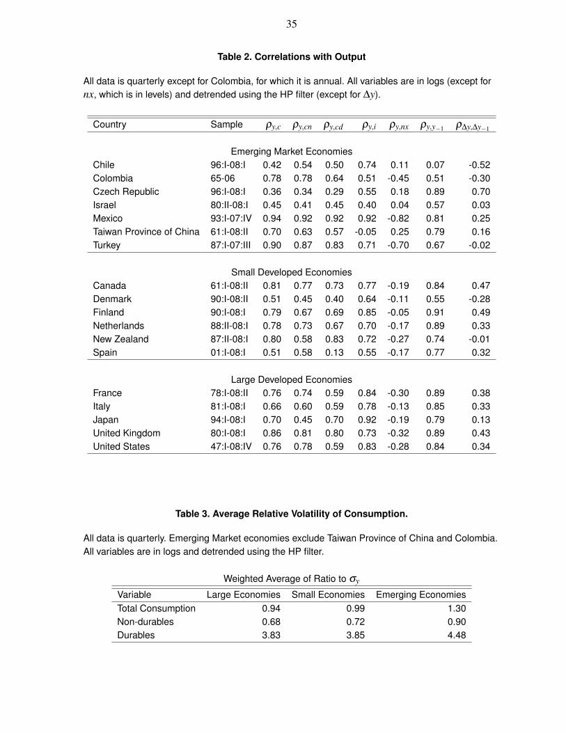
Table 2. Correlations with Output
All data is quarterly except for Colombia, for which it is annual. All variables are in logs (except fornx, which is in levels) and detrended using the HP filter (except for ∆y).
Country Sample ρy,c ρy,cn ρy,cd ρy,i ρy,nx ρy,y−1 ρ∆y,∆y−1
Emerging Market EconomiesChile 96:I-08:I 0.42 0.54 0.50 0.74 0.11 0.07 -0.52Colombia 65-06 0.78 0.78 0.64 0.51 -0.45 0.51 -0.30Czech Republic 96:I-08:I 0.36 0.34 0.29 0.55 0.18 0.89 0.70Israel 80:II-08:I 0.45 0.41 0.45 0.40 0.04 0.57 0.03Mexico 93:I-07:IV 0.94 0.92 0.92 0.92 -0.82 0.81 0.25Taiwan Province of China 61:I-08:II 0.70 0.63 0.57 -0.05 0.25 0.79 0.16Turkey 87:I-07:III 0.90 0.87 0.83 0.71 -0.70 0.67 -0.02
Small Developed EconomiesCanada 61:I-08:II 0.81 0.77 0.73 0.77 -0.19 0.84 0.47Denmark 90:I-08:II 0.51 0.45 0.40 0.64 -0.11 0.55 -0.28Finland 90:I-08:I 0.79 0.67 0.69 0.85 -0.05 0.91 0.49Netherlands 88:II-08:I 0.78 0.73 0.67 0.70 -0.17 0.89 0.33New Zealand 87:II-08:I 0.80 0.58 0.83 0.72 -0.27 0.74 -0.01Spain 01:I-08:I 0.51 0.58 0.13 0.55 -0.17 0.77 0.32
Large Developed EconomiesFrance 78:I-08:II 0.76 0.74 0.59 0.84 -0.30 0.89 0.38Italy 81:I-08:I 0.66 0.60 0.59 0.78 -0.13 0.85 0.33Japan 94:I-08:I 0.70 0.45 0.70 0.92 -0.19 0.79 0.13United Kingdom 80:I-08:I 0.86 0.81 0.80 0.73 -0.32 0.89 0.43United States 47:I-08:IV 0.76 0.78 0.59 0.83 -0.28 0.84 0.34
Table 3. Average Relative Volatility of Consumption.
All data is quarterly. Emerging Market economies exclude Taiwan Province of China and Colombia.All variables are in logs and detrended using the HP filter.
Weighted Average of Ratio to σy
Variable Large Economies Small Economies Emerging EconomiesTotal Consumption 0.94 0.99 1.30Non-durables 0.68 0.72 0.90Durables 3.83 3.85 4.48
36
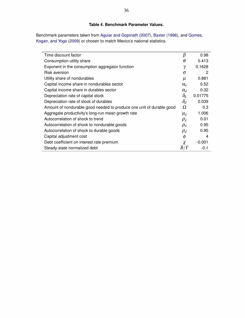
Table 4. Benchmark Parameter Values.
Benchmark parameters taken from Aguiar and Gopinath (2007), Baxter (1996), and Gomes,Kogan, and Yogo (2009) or chosen to match Mexico’s national statistics.
Time discount factor β 0.98Consumption utility share θ 0.413Exponent in the consumption aggregator function γ 0.1628Risk aversion σ 2Utility share of nondurables µ 0.881Capital income share in nondurables sector αn 0.52Capital income share in durables sector αd 0.32Depreciation rate of capital stock δk 0.01775Depreciation rate of stock of durables δd 0.039Amount of nondurable good needed to produce one unit of durable good Ω 0.3Aggregate productivity’s long-run mean growth rate µg 1.006Autocorrelation of shock to trend ρg 0.01Autocorrelation of shock to nondurable goods ρn 0.95Autocorrelation of shock to durable goods ρd 0.95Capital adjustment cost φ 4Debt coefficient on interest rate premium χ -0.001Steady-state normalized debt B/Y -0.1
37
Table 5. Simulated moments and parameter estimates for Mexico
Simulated moments for GDP (y), first difference of GDP (∆y), nondurables production (yn), durables production (yd ),total consumption expenditure (c), consumption of nondurables (cn), investment in capital goods (i), durable goodsexpenditure (cd), the borrowing premium (bp), and net exports-output ratio (nx). Standard deviations for all variables(except y, ∆y and nx) are relative to that of output. Data for nondurable and durable production is for industrial produc-tion and comes from INEGI. Data for the borrowing premium is from Neumeyer and Perri (2005) Results in column (1)through (5) were obtained by solving for the parameters with values in bold in order to match the sample moments withvalues in bold. Unless otherwise specified, parameters are set at their benchmark values (see Table 4).
No Financial Frictions Financial FrictionsData ( 1) ( 2) ( 3) ( 4) ( 5)
σy 2.35 2.3500 2.3579 2.3500 2.3500 2.4056σ∆y 1.50 1.7648 1.7564 1.7746 1.7557 1.8012σyn 0.93 0.8988 1.0266 0.9829 0.8988 0.8883σyd 3.31 1.6325 1.0137 1.2299 1.6325 1.6678σc 1.10 1.0267 1.0025 1.1000 1.0588 1.0404σcn 0.89 0.8900 1.0351 0.9844 0.8900 0.8780σcd 4.20 4.2000 0.9083 4.0090 4.2000 4.2399σi 6.11 3.2811 3.6215 2.9470 3.6380 3.4737σnx 1.68 1.6800 1.6689 1.6800 1.6800 1.6234σbp 2.64 0.9287 0.9884 0.9262 3.3503 2.6501ρy,y−1 0.81 0.7432 0.7523 0.7397 0.7461 0.7441ρ∆y,∆y−1 0.25 0.0353 0.0662 0.0311 0.0373 0.0327ρyn,y 0.71 0.9494 0.9923 0.9810 0.9493 0.9467ρyd ,y 0.80 0.8693 0.9339 0.8963 0.8693 0.8718ρc,y 0.92 0.9237 0.9930 0.9525 0.9424 0.9374ρcn,y 0.92 0.9201 0.9884 0.9709 0.9201 0.9155ρcd,y 0.92 0.5706 0.7573 0.5179 0.7143 0.6820ρi,y 0.94 0.7659 0.7120 0.7045 0.8740 0.8595ρnx,y -0.82 -0.4468 -0.5245 -0.4076 -0.7206 -0.6688ρbp,y -0.49 0.5639 0.5040 0.5175 -0.4900 -0.4876ρlab,y 0.90 0.7557 0.4937 0.7454 0.7976 0.8147ρyd ,yn 0.67 0.6700 0.8825 0.7931 0.6700 0.6675
Quality of Fit 0.8363 0.7160 0.7978 0.8969 0.8939σg 1.8340 2.4776 1.9107 1.5795 1.5410σn 1.4209 1.4461 1.5897 1.4743 1.5164σd 1.4528 0.0000 0.8211 1.6428 1.6956ψ 0.5336 0 0.5336 0.6231 0.5213ρnd 0.3631 0.3631 0.3631 0.4702 0.4660η 0 0 0 -0.0077 -0.0059σb 0 0 0 0 0.0000δd 0.039 0.99 0.039 0.039 0.039wn 0.2779 0.4054 0.2500 0.2091 0.1921wd 0.4266 1.0202 0.7238 0.3001 0.2768Share of εg in GDPvariance decomposition (%) 0.3300 0.5722 0.3684 0.2405 0.2185
38
Table 6. Simulated moments and parameter estimates for an alternative specifications of theborrowing premium
χ =−.0005 χ =−.001 χ =−.0015σy 2.3198 2.3436 2.3630σ∆y 1.7386 1.7501 1.7588σyn 0.8948 0.8980 0.9005σyd 1.6466 1.6354 1.6266σc 1.0253 1.0392 1.0464σcn 0.8854 0.8890 0.8919σcd 4.1305 4.1851 4.2304σi 3.5447 3.5207 3.4480σnx 1.7007 1.6846 1.6709σbp 2.6406 2.6401 2.6400ρy,y−1 0.7436 0.7459 0.7480ρ∆y,∆y−1 0.0310 0.0350 0.0407ρyn,y 0.9483 0.9491 0.9498ρyd ,y 0.8702 0.8695 0.8690ρc,y 0.9332 0.9358 0.9343ρcn,y 0.9182 0.9197 0.9208ρcd,y 0.6214 0.6466 0.6446ρi,y 0.7924 0.8186 0.8276ρnx,y -0.5402 -0.5918 -0.5975ρbp,y -0.4901 -0.4900 -0.4898ρlab,y 0.7901 0.7900 0.7869ρyd ,yn 0.6687 0.6697 0.6705σg 1.4106 1.5963 1.7643σn 1.4970 1.4716 1.4441σd 1.5960 1.5767 1.5298ρnd 0.4488 0.4295 0.3996ηg 0.0137 0.0098 -0.0053ηn -0.0051 -0.0080 -0.0097ηd -0.0070 -0.0068 -0.0059Share of εg in GDPvariance decomposition 0.0976 0.1317 0.1667