Business Cycles in Emerging Economies: The Role of InterestRates∗

Pablo A. Neumeyer

Universidad T. di Tella and CONICET

Fabrizio Perri∗∗

New York UniversityFederal Reserve Bank of Minneapolis

NBER and CEPR

March 2004

ABSTRACT

We find that in a sample of emerging economies business cycles are more volatile than in developed ones, realinterest rates are countercyclical and lead the cycle, consumption is more volatile than output and net exportsare strongly countercyclical. We present a model of a small open economy, where the real interest rate isdecomposed in an international rate and a country risk component. Country risk is affected by fundamentalshocks but, through the presence of working capital, also amplifies the effects of those shocks. The modelgenerates business cycles consistent with Argentine data. Eliminating country risk lowers Argentine outputvolatility by 27% while stabilizing international rates lowers it by less than 3%.

keywords: Country risk, financial crises, international business cycles, sudden stops, working capital

jel classification codes: E32, F32, F41

∗ We thank Paco Buera and Rodolfo Campos for excellent research assistance, the associate editor, an anonymousreferee, Fernando Alvarez, Isabel Correia, Patrick Kehoe, Enrique Mendoza, Juan Pablo Nicolini, Martin Schneider,Pedro Teles, Ivan Werning, and participants at several seminars and conferences for helpful suggestions. We are alsograteful for the financial support of the Tinker Foundation and the Agencia de Promoción Científica y Tecnológica(Pict 98 Nro. 02-03543) and to the department of economics at the Stern School of Business for hosting Neumeyer inthe Spring of 1999. The views expressed here are those of the authors and not necessarily those of the FederalReserve Bank of Minneapolis or the Federal Reserve System∗∗ Corresponding author. Tel.: +1 (612) 204-5484; fax: +1 (612) 204 5515E-Mail address: fperri@stern.nyu.edu

1. Introduction

In recent years a large number of emerging economies have faced frequent and large changes

in the real interest rates they face in international financial markets; these changes have usually been

associated with large business cycle swings. The virulence of these crises has prompted proposals to

enact policies that would stabilize international credit conditions for emerging markets. This paper

is motivated by this observation and has two objectives. The first is to systematically document

the relation between real interest rates and business cycles in emerging economies and to contrast it

with the relation we observe for developed countries. The second is to lay out a model that is helpful

in understanding and quantifying the nature of this relation. In particular we seek to measure the

contribution of real interest rate fluctuations to the high volatility of output in emerging economies.

This is useful to asses the effectiveness of policies that seek to moderate business cycles in emerging

markets by stabilizing real interest rates.

We start with a statistical analysis of business cycles in a set of small open emerging economies

(Argentina, Brazil, Mexico, Korea, and Philippines) on one hand and a set of small open developed

economies (Australia, Canada, Netherlands, New Zealand, and Sweden) on the other. The data

show that many features of business cycles are similar in the two sets of economies, but that there

are also some notable differences. In emerging economies real interest rates are countercyclical and

lead the business cycle. In contrast, real rates in developed economies are acyclical and lag the cycle.

Also, emerging economies display high, relative to developed economies, output volatility, and the

volatility of consumption relative to income is on average greater than one and higher than in the

developed economies. Finally, net exports appear much more strongly countercyclical in emerging

economies than in developed economies.

The strong relation between interest rates and business cycles in emerging economies is at

odds with the minor role played by interest rate shocks in previous models of business cycles in

small open economies. Quantitative exercises performed in this class of models show that interest

rate disturbances do not play a significant role in driving business cycles (see Mendoza, 1991, and

Correia et al., 1995). Moreover, in these models interest rates are either acyclical or procyclical,

consumption is less volatile than output, and countercyclicality of net exports is mild.

We introduce two simple modifications to an otherwise standard neoclassical framework in

order to have a model of business cycles that is consistent with the main empirical regularities

of emerging economies and, in particular, with the cyclical properties of interest rates. The first

modification is that firms have to pay for part of the factors of production before production takes

place, creating a need for working capital. The second modification (common in the small open

economy business cycle literature) is that we consider preferences which generate a labor supply

that is independent of consumption. These two modifications generate the transmission mechanism

by which real interest rates affect the level of economic activity. The need for working capital to

finance the wage bill makes the demand for labor sensitive to the interest rate. Since firms have to

borrow to pay for inputs, increases in the interest rate make their effective labor cost higher and

reduce their labor demand for any given real wage. The impact of this fall in labor demand on

equilibrium employment will depend on the nature of the labor supply. Our preference specification

guarantees that the labor supply is independent of shocks to interest rates. Hence, declines in labor

demand induce a fall in equilibrium employment that depends on the elasticity of the labor supply

with respect to the real wage. Because at business cycle frequencies the capital stock is relatively

stable, declines in equilibrium employment translate into output declines.

We then use the dynamic general equilibrium model of a small open economy with working

capital to assess quantitatively the role of interest rates in driving business cycles. In order to do

so, we calibrate our model to Argentina’s economy for the period 1983-2001; we chose Argentina

because it is the country for which the longest relevant interest rate series is available.

2

One important issue we have to model is the nature of interest rate fluctuations. the interest

rate faced by an emerging economy is the sum of two independent components: an international

rate plus a country risk spread. We identify the international rate relevant for emerging economies

as the rate on non-investment-grade bonds in the United States. We then construct the country risk

spread as the difference between the rate faced by emerging economies and this international rate.

Because fluctuations in country risk spreads are large, we consider two simple polar (non-mutually

exclusive) approaches to their determination. The first is that factors that are largely independent

of domestic conditions (like foreign rates, contagion, or political factors) drive country risk. In

the second approach changes in country risk are induced by the fundamental shocks to a country’s

economy (productivity shocks in our model). In this case, these shocks drive, at the same time,

business cycles and fluctuations in country risk.

Our first finding is that the quantitative results from the model with productivity shocks

and country risk induced by productivity shocks can account for most empirical regularities (second

moments of national account components and interest rates) of Argentina’s economy during the

period. This suggests that country risk is induced by domestic fundamentals but that at the same

time, through the presence of working capital, amplifies the effects of fundamental shocks on business

cycles. Given our first result we can use the model to assess how much business cycle volatility

would be reduced by eliminating interest rate fluctuations. We find that eliminating fluctuation in

country risk would lower gross domestic product (GDP) volatility by around 27%, while eliminating

international real rate fluctuations would lower volatility by less than 3%. Our results lead us

to think that in order to understand business cycle volatility in emerging economies, it is crucial

to understand the exact mechanism through which shocks to fundamentals induce fluctuations in

country risk.

Our work builds on related empirical and quantitative work on business cycles in emerging

3

and developed countries. Our findings on the empirical regularities of business cycles are consistent

with those of Backus and Kehoe (1992), Mendoza (1995), and Agenor et al. (2000), among others,

who find that, although the magnitude of output fluctuations has varied across countries (with less

developed countries displaying larger fluctuations) and periods, the co-movements of consumption,

investment, and net exports with output during the cycle are quite uniform. Recently, Uribe and

Yue (2003) have investigated the relation between international interest rates, country spreads,

and output fluctuations in a sample of seven emerging economies, and they find a strong negative

correlation between real interest rates and economic activity.

There are three strands of quantitative business cycle literature that are related to this paper:

the first is the one that studies the effects of “sudden stops”1 in capital flows on economic activity

in emerging economies, the second is the one that focuses on the business cycle associated with

exchange rate based stabilizations, and the third one studies the effect on business cycles of shocks

to the wedge between the marginal product of labor and the consumption-leisure marginal rate of

substitution.

As we do in this paper, the quantitative literature on the economics of “sudden stops” (see

Mendoza and Smith, 2002, and Christiano, et al., 2003, among others) highlights the importance

of external financial factors for macroeconomic developments in emerging economies. These models

study the effect of the sudden imposition of an external credit constraint on business cycles. In

these models, when the credit constraint suddenly binds, domestic interest rates rise, output drops,

and there is a dramatic increase in the current account surplus (the “sudden stop” in capital flows).

This paper looks at the effect of external financial conditions on economic activity through prices

instead of quantities.

The literature that focuses on the business cycles associated to exchange rate based stabi-

1The term “sudden stops” refers to sudden stops in capital flows to emerging economies (see Calvo, 1998).

4

lization plans (see Rebelo and Vegh, 1995, and Calvo and Vegh, 1999) argues that current theories

cannot account for the magnitude of the fluctuations in economic activity observed at the onset and

at the end of a stabilization plan. The quantitative exercise carried out in this paper suggests that

fluctuations in country risk might provide the amplification mechanism needed to reconcile data and

theory. In the case of Argentina, for example, the stabilization plans that fall within our sample are

the Austral Plan that started in June 1985 and the Currency Board that started in April 1991. In

both events the business cycle expansion that characterized the start of the plan was also associated

with declines in the real interest rate. Conversely, the recessions that hit the country at the end of

the plans were associated with interest rate spikes.

In the closed economy literature, Cooley and Hansen (1989) and Christiano and Eichenbaum

(1992) study the effect of shocks to the wedge between the consumption-leisure marginal rate of

substitution and the marginal product of labor. In Cooley and Hansen, this wedge stems from a

cash-in-advance constraint, and it is equal to the nominal interest rate (the inflation tax). Christiano

and Eichenbaum create this wedge, as we do, by assuming that firms must borrow working capital

to finance labor costs. In our experiment real interest rates affect the same margin as in the articles

cited above, but have different causes (country risk instead of monetary policy) and different effects

due to the different specification of preferences. It is worth emphasizing that our model is non-

monetary and that the distortion introduced by the firm’s need for working capital depends on

real interest rates and not on nominal ones. If we had used nominal interest rates as the source of

distortion, the model would have predicted large output fluctuations in the 1980s (when Argentine

inflation was extremely volatile) (see Neumeyer, 1998) but almost no movement in the 1990s when

inflation was virtually zero.2

2Uribe (1997) uses the same margin as Cooley and Hansen, with a nominal distortion, to generate the outputexpansion that follows an exchange rate based stabilization plan.

5

2. Real interest rates and business cycles in emerging economies

This section documents empirical regularities about business cycles and real interest rates

in the five small open emerging economies for which we could obtain comparable real interest rate

time series: Argentina, Brazil, Korea, Mexico, and Philippines. To highlight the features of business

cycles that are special to emerging economies, we also document the same facts for five small open

developed economies: Australia, Canada, Netherlands, New Zealand, and Sweden. The sample has

a quarterly frequency, starts in the third quarter of 1983, and ends in the last quarter of 2001 for

Argentina and the developed economies. For the other emerging economies, it starts in the first

quarter of 1994.3

2.1. Data description

The data we use to compute business cycle statistics are standard and were obtained from

the Organisation for Economic Co-operation and Development (OECD) and local national accounts

sources (see the Data Appendix for more details). The interest rate we want to measure is the

expected 3-month real interest rate at which firms in a country can borrow. This rate is easily

constructed for developed economies (see the Data Appendix) but is more difficult to obtain for

emerging economies. Some local sources report local currency nominal interest rates, but the high

variability of local inflation in same cases makes it hard to derive a measure of domestic expected

inflation needed to construct the real interest rate.4 Other sources report interest rate data on new

loans denominated in U.S. dollars, so the real interest rate can be computed without computing

3Our sample for emerging economies is limited both in terms of countries and in terms of time span. The limitationstems from the fact that we construct interest rate series using dollar denominated bond prices or indexes. To ourknowledge, Argentina is the only country for which there are data on bond prices going back to the 1980s since itissued four 10-year dollar denominated sovereign coupon bonds between 1980 and 1984. We start our sample in thethird quarter of 1983 because it is the first quarter for which we have at least three bond prices. Brazil, Korea, Mexico,and Philippines are the non-oil exporting countries with the longest data series in the data set of dollar denominatedbonds index (EMBI) constructed by J.P. Morgan.

4 In Argentina, for example, inflation swings from one month to the next reached over 1000% per year. As aconsequence measures of expected inflation constructed using actual inflation are also very volatile and imply volatileand, sometimes, implausibly negative real interest rates.

6

domestic expected inflation; the problem with those series is that during financial crises most of

the new borrowing of emerging countries is through official institutions, and thus recorded interest

rates do not reflect the true intertemporal terms of trade faced by local private agents.5 For these

reasons we use secondary market prices of emerging market bonds to recover nominal U.S. dollar

interest rates and obtain real rates by subtracting expected U.S. inflation. Since these bonds are

traded on international financial markets, they reflect the intertemporal terms of trade locals face on

these markets, and, since they are dollar denominated, real interest rates can be computed without

constructing domestic expected inflation.6 More precisely for Argentina we construct interest rates

using a combination of government bonds issued from 1980 onward and the EMBI, while for the

other emerging economies we use only the EMBI. (See the Data Appendix for more details on the

construction of interest rates.) One last issue is that the interest rates we construct are primarily

based on government bonds, and private firms might, in principle, face a very different rate. In

order to check that this is not the case, we obtained for Argentina a dollar denominated prime

corporate rate that is relevant for the private sector and that we can directly compare with the rate

we construct.7 Although the two rates are not identical, they have very similar magnitudes and

they track each other very closely with a correlation of 0.89.

2.2. Business cycle statistics

The main result of this section is that business cycles in these two sets of economies differ

along some important dimensions. In contrast to developed economies, in the emerging economies

we study, real interest rates are countercyclical and they lead the cycle. The emerging economies are

also more volatile than the developed ones because the volatilities of output, real interest rates, and

5For example, the World Bank Global Development Finance reports an average interest rate on new loans toArgentina of only 6% during the hyperinflation of the 1990s and of 7% during the Tequila Crisis of 1994-95.

6The interest rates on dollar (foreign currency) denominated assets are also relevant for domestic agents as long asthere are no large and predictable changes in purchasing power parity.

7The 90-day, dollar denominated, prime corporate rate in Argentina is from Boletín Estadístico, Banco Central dela República Argentina. The reason we do not use this rate directly is that it is available only starting in 1994.

7

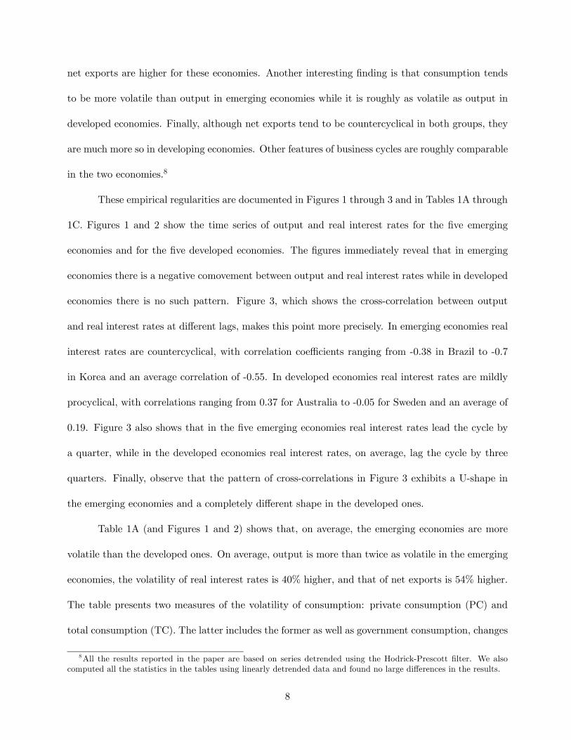
net exports are higher for these economies. Another interesting finding is that consumption tends

to be more volatile than output in emerging economies while it is roughly as volatile as output in

developed economies. Finally, although net exports tend to be countercyclical in both groups, they

are much more so in developing economies. Other features of business cycles are roughly comparable

in the two economies.8

These empirical regularities are documented in Figures 1 through 3 and in Tables 1A through

1C. Figures 1 and 2 show the time series of output and real interest rates for the five emerging

economies and for the five developed economies. The figures immediately reveal that in emerging

economies there is a negative comovement between output and real interest rates while in developed

economies there is no such pattern. Figure 3, which shows the cross-correlation between output

and real interest rates at different lags, makes this point more precisely. In emerging economies real

interest rates are countercyclical, with correlation coefficients ranging from -0.38 in Brazil to -0.7

in Korea and an average correlation of -0.55. In developed economies real interest rates are mildly

procyclical, with correlations ranging from 0.37 for Australia to -0.05 for Sweden and an average of

0.19. Figure 3 also shows that in the five emerging economies real interest rates lead the cycle by

a quarter, while in the developed economies real interest rates, on average, lag the cycle by three

quarters. Finally, observe that the pattern of cross-correlations in Figure 3 exhibits a U-shape in

the emerging economies and a completely different shape in the developed ones.

Table 1A (and Figures 1 and 2) shows that, on average, the emerging economies are more

volatile than the developed ones. On average, output is more than twice as volatile in the emerging

economies, the volatility of real interest rates is 40% higher, and that of net exports is 54% higher.

The table presents two measures of the volatility of consumption: private consumption (PC) and

total consumption (TC). The latter includes the former as well as government consumption, changes

8All the results reported in the paper are based on series detrended using the Hodrick-Prescott filter. We alsocomputed all the statistics in the tables using linearly detrended data and found no large differences in the results.

8

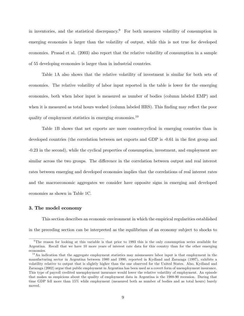
in inventories, and the statistical discrepancy.9 For both measures volatility of consumption in

emerging economies is larger than the volatility of output, while this is not true for developed

economies. Prasad et al. (2003) also report that the relative volatility of consumption in a sample

of 55 developing economies is larger than in industrial countries.

Table 1A also shows that the relative volatility of investment is similar for both sets of

economies. The relative volatility of labor input reported in the table is lower for the emerging

economies, both when labor input is measured as number of bodies (column labeled EMP) and

when it is measured as total hours worked (column labeled HRS). This finding may reflect the poor

quality of employment statistics in emerging economies.10

Table 1B shows that net exports are more countercyclical in emerging countries than in

developed countries (the correlation between net exports and GDP is -0.61 in the first group and

-0.23 in the second), while the cyclical properties of consumption, investment, and employment are

similar across the two groups. The difference in the correlation between output and real interest

rates between emerging and developed economies implies that the correlations of real interest rates

and the macroeconomic aggregates we consider have opposite signs in emerging and developed

economies as shown in Table 1C.

3. The model economy

This section describes an economic environment in which the empirical regularities established

in the preceding section can be interpreted as the equilibrium of an economy subject to shocks to

9The reason for looking at this variable is that prior to 1993 this is the only consumption series available forArgentina. Recall that we have 10 more years of interest rate data for this country than for the other emergingeconomies.10An indication that the aggregate employment statistics may mismeasure labor input is that employment in the

manufacturing sector in Argentina between 1980 and 1990, reported in Kydland and Zarazaga (1997), exhibits avolatility relative to output that is slightly higher than the one observed for the United States. Also, Kydland andZarazaga (2002) argue that public employment in Argentina has been used as a covert form of unemployment insurance.This type of payroll credited unemployment insurance would lower the relative volatility of employment. An episodethat makes us suspicious about the quality of employment data in Argentina is the 1988-90 recession. During thattime GDP fell more than 15% while employment (measured both as number of bodies and as total hours) barelymoved.

9

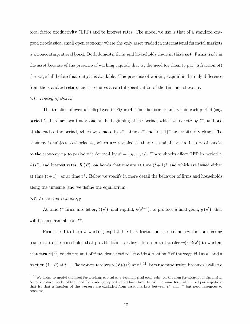
total factor productivity (TFP) and to interest rates. The model we use is that of a standard one-

good neoclassical small open economy where the only asset traded in international financial markets

is a noncontingent real bond. Both domestic firms and households trade in this asset. Firms trade in

the asset because of the presence of working capital, that is, the need for them to pay (a fraction of)

the wage bill before final output is available. The presence of working capital is the only difference

from the standard setup, and it requires a careful specification of the timeline of events.

3.1. Timing of shocks

The timeline of events is displayed in Figure 4. Time is discrete and within each period (say,

period t) there are two times: one at the beginning of the period, which we denote by t−, and one

at the end of the period, which we denote by t+. times t+ and (t + 1)− are arbitrarily close. The

economy is subject to shocks, st, which are revealed at time t−, and the entire history of shocks

to the economy up to period t is denoted by st = (s0, ..., st). These shocks affect TFP in period t,

A(st), and interest rates, R¡st¢, on bonds that mature at time (t+1)+ and which are issued either

at time (t+1)− or at time t+. Below we specify in more detail the behavior of firms and households

along the timeline, and we define the equilibrium.

3.2. Firms and technology

At time t− firms hire labor, l¡st¢, and capital, k(st−1), to produce a final good, y

¡st¢, that

will become available at t+.

Firms need to borrow working capital due to a friction in the technology for transferring

resources to the households that provide labor services. In order to transfer w(st)l(st) to workers

that earn w(st) goods per unit of time, firms need to set aside a fraction θ of the wage bill at t− and a

fraction (1−θ) at t+. The worker receives w(st)l(st) at t+.11 Because production becomes available

11We chose to model the need for working capital as a technological constraint on the firm for notational simplicity.An alternative model of the need for working capital would have been to assume some form of limited participation,that is, that a fraction of the workers are excluded from asset markets between t− and t+ but need resources toconsume.

10

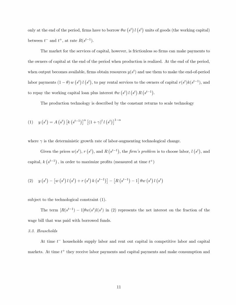
only at the end of the period, firms have to borrow θw¡st¢l¡st¢units of goods (the working capital)

between t− and t+, at rate R(st−1).

The market for the services of capital, however, is frictionless so firms can make payments to

the owners of capital at the end of the period when production is realized. At the end of the period,

when output becomes available, firms obtain resources y(st) and use them to make the end-of-period

labor payments (1− θ)w¡st¢l¡st¢, to pay rental services to the owners of capital r(st)k(st−1), and

to repay the working capital loan plus interest θw¡st¢l¡st¢R¡st−1

¢.

The production technology is described by the constant returns to scale technology

(1) y¡st¢= A

¡st¢ £k¡st−1

¢¤α £(1 + γ)t l

¡st¢¤1−α

where γ is the deterministic growth rate of labor-augmenting technological change.

Given the prices w(st), r¡st¢, and R

¡st−1

¢, the firm’s problem is to choose labor, l

¡st¢, and

capital, k¡st−1

¢, in order to maximize profits (measured at time t+)

(2) y¡st¢−£w¡st¢l¡st¢+ r

¡st¢k¡st−1

¢¤−£R¡st−1

¢− 1¤θw¡st¢l¡st¢

subject to the technological constraint (1).

The term [R(st−1) − 1]θw(st)l(st) in (2) represents the net interest on the fraction of the

wage bill that was paid with borrowed funds.

3.3. Households

At time t− households supply labor and rent out capital in competitive labor and capital

markets. At time t+ they receive labor payments and capital payments and make consumption and

11

investment decisions. Their preferences are described by the expected utility

(3)∞Xt=0

Xst

βtπ¡st¢u¡c¡st¢, l¡st¢¢

where π¡st¢is the probability of history st occurring conditional on the information set at time

t = 0, 0 < β < 1 is the constant discount factor, and c¡st¢is consumption. The household’s budget

constraints are then given by

(4) c(st) + x(st) + b(st) + κ¡b¡st¢¢≤ w(st)l(st) + r(st)k(st−1) + b(st−1)R

¡st−1

¢

for all st.

At time t+ households spend the proceeds from bond holdings b¡st−1

¢R¡st−1

¢and their

labor and capital income on consumption, investment x(st), bond purchases b(st), and the cost of

holding bonds, κ¡b¡st−1

¢¢, where κ (·) is a convex function.12

The resources used for investment x(st) add to the current stock of capital and are used to

cover a capital adjustment cost

(5) x(st) = k(st)− (1− δ)k(st−1) +Φ(k(st−1), k(st))

for all st, where the function Φ represents the cost of adjusting the capital stock. Adjustment costs

such as these are commonly used in the business cycle literature of small open economies in order

to avoid excessive volatility of investment.

The household’s problem then is to choose the state-contingent sequences of consumption,

12The quantitative experiments performed in the next section are computed linearizing the model around its steadystate value. Bond holding costs are needed to guarantee that bond holdings do not display a unit root. See Schmitt-Grohé and Uribe (2003) for alternative ways of obtaining this. The parameters of the function κ are chosen so thatthese costs are minimal and do not affect the short-run properties of the model.

12

c¡st¢, labor, l

¡st¢, bond holdings, b

¡st¢, and investment, x

¡st¢, that maximize the expected utility

(3) subject to the sequence of budget constraints (4), the capital accumulation constraints (5), and

a no-Ponzi-game condition, for given values of the initial levels of capital and debt, k (0) and b (0) ,

and for the given sequences of prices, w(st), r¡st¢, and R

¡st¢.

3.4. Equilibrium allocations and prices

Given initial conditions k (0) and b (0), a state-contingent sequence of interest rates R¡st¢,

and TFP A(st), an equilibrium is a state-contingent sequence of allocations {c¡st¢, l¡st¢, b¡st¢,

x¡st¢, k

¡st¢} and of prices {w(st), r

¡st¢} such that (i) the allocations solve the firm’s and the

household’s problem at the equilibrium prices and (ii) markets for factor inputs clear. A balanced

growth path for the economy is an equilibrium in which R¡st¢, A(st) are constant. Along a balanced

growth path r(st) and l(st) are constant and all other variables grow at rate γ.

Because this is a small open economy, the household’s asset position, b¡st−1

¢net of the firm’s

working capital debt, θw¡st¢l¡st¢, is the country’s net foreign asset position in period t. Similarly,

the goods produced in the country that are not spent in consumption, investment, or bond holding

costs are the country’s net exports.

The parameter θ captures the importance of working capital. If it is set to zero, firms do

not need working capital, the term capturing the cost of the working capital in the firm’s profit

function, (2), disappears, and the model reduces exactly to the standard neoclassical one.

4. Interest rates and country risk

The model economy described in the preceding section is subject to interest rate and pro-

ductivity shocks. As we discussed in Section 2, the interest rates faced by emerging economies are

quite volatile. In this section we provide a simple theory of this interest rate volatility in emerging

economies.

We assume that a large mass of international investors is willing to lend to the emerging

13

economy any amount at a rate R(st). Loans to the domestic economy are risky assets because we

assume that there can be default on payments to foreigners. This assumption creates two sources

of volatility in R: first, real interest rates change as the perceived default risk changes; second, even

if the default risk stays constant, interest rates can change because the preference of international

investors for risky assets might change over time. We capture these two sources of interest rate

volatility by decomposing the interest rate faced by the emerging economy as

(6) R(st) = R∗¡st¢D(st)

where R∗ is an international rate for risky assets (which is not specific to any emerging economy) and

D measures the country spread over R∗ paid by borrowers in a particular economy. One important

issue is how to model default decisions. To keep matters very simple, we assume that private

domestic lenders always pay their obligation in full but that in each period there is a probability

that the local government will confiscate all the interest payments going from local borrowers to

the foreign lenders.13 Time variation in this confiscation probability will cause time variation in the

country spreads D.

In our computational experiments domestic firms borrow funds from domestic households and

from foreign investors. The existence of only one asset implies that all agents (domestic or foreign,

borrower or lender) face the same rate of interest R. The small open economy assumption implies

that the interest rate on this internationally traded bond is determined by the foreign bond holders

that are subject to default risk. Domestic lenders always receive back the full value of their loan

plus interest. Thus, our assumptions on interest rates are fully consistent with the model described

in the preceding section as long as foreigners lend positive amounts to the domestic economy all

13Kehoe and Perri (2004) model international default in a similar fashion.

14

along the equilibrium path. 14

Throughout the paper we will identify R∗ as a U.S. rate for risky assets and model it as a

stochastic process completely independent from conditions in the emerging economy (see Section

5).

The more important issue to resolve though is what drives fluctuations in the confiscation

probability in a particular economy and hence in its country spread D. A complete model of the

determination of fluctuations in country risk is beyond the scope of this paper, because our main

goal is to analyze the relation between interest rates and business cycles. However, a minimal model

of country risk is necessary to conduct our quantitative analysis. In the rest of the paper, we consider

two polar (non-mutually exclusive) approaches.

The first approach is that exogenous factors (like foreign events, contagion, or political factors

that are largely independent of local productivity shocks) also drive country risk. Under this view,

the interest rate R is determined by two separate stochastic processes (chosen to replicate observed

data) that are both independent from the fundamentals of the economy in question. We refer to

this approach as the independent country risk case.

The second approach is that fundamental shocks to a country’s economy (productivity shocks

in our model) drive the business cycle and country risk at the same time. The simplest way to model

this is to assume that default probabilities and, hence, country risk are a function of productivity

shocks. This idea is based on models of default and incomplete markets (see, for example, Eaton

and Gersovitz, 1981, or more recently Arellano, 2003) in which default probabilities are high when

expectations of productivity shocks are low. Thus, the country risk component of R(st) (which is

known in period t but is the rate at which firms borrow in period t+ 1) is a decreasing function of

14 In our computational experiments we check that this condition is always satisfied.

15

expected productivity in t+ 1

(7) D¡st¢= η

¡EtA

¡st+1

¢¢.

This reduced form approach to endogenous default is subject to the usual critiques since the function

η (·) may itself depend on other economic fundamentals. The purpose of introducing this relation is

not to provide a satisfactory model of country risk, but only to show that country risk, even when

it is fully determined by local fundamental economic conditions, can act as a powerful amplification

mechanism. Under this approach, the driving forces of fluctuations are the realization of shocks

to productivity and to international real interest rates. We refer to this approach as the induced

country risk case.

5. Calibration of shock processes and parameters

The objective of the computational experiments performed in Section 6 is to evaluate the

role played by interest rates in the business cycles of emerging economies and contrast it with the

role played by productivity shocks. To that end we need to calibrate the parameters of the model

and the stochastic processes for country risk, international real interest rates, and productivity

shocks. A period in the model is assumed to be a quarter. We will use data from Argentina for

the period 1983-2001. We will first describe how we model total factor productivity, then how we

obtain processes for interest rates, and finally, how we calibrated other parameters. From now on

we let x denote the percentage deviation of variable x from its balanced growth path.

5.1. Total factor productivity

Estimating a reliable process for the shocks to total factor productivity for our experiments

entails the estimation of a reliable series for Argentina’s Solow residuals with a quarterly frequency.

Unfortunately, this is impossible at the quarterly level since labor statistics in Argentina are collected

16

at semi-annual frequencies. Furthermore, the available labor statistics may not measure accurately

labor inputs as discussed in Section 3. Because of these issues we simply assume that the process

for percentage deviations from trend of total factor productivity, A(st), follow the AR(1) process

(8) A¡st¢= ρA A

¡st−1

¢+ εA

¡st¢

and assume that it has the same persistence as the process estimated for the United States with

ρA = 0.95. We assume that innovations to productivity εA¡st¢are normally distributed and serially

uncorrelated and, in the experiments in which productivity shocks are turned on, set their volatility

so that the simulated volatility of output in the experiments we conduct matches the Argentine

data.

5.2. Interest rates

Country risk, D¡st¢, is defined as the ratio between Argentine rates, R(st), and international

interest rates, R∗¡st¢, as in (6). We measure R(st) as the 3-month real yield on Argentine dollar

denominated sovereign bonds (as discussed in the data section, this rate is a good approximation

for the rate faced by Argentine firms) and R∗¡st¢as the redemption real yield on an index on non-

investment-grade U.S. domestic bonds. Since Argentine sovereign bonds are also non-investment-

grade a change in the difference between R(st) and R∗¡st¢should capture a change in Argentina’s

idiosyncratic default risk and not a change in the overall risk preference of international (U.S.)

investors. Figure 5 shows the evolution of R and R∗ over the sample period. Note how in “tranquil

times” (for example, the early ’90s) the rate faced by Argentina is very close to the U.S. risky rate,

while during crisis times (for example, the hyperinflation of 1989) country risk goes up significantly.

Because we find that R∗(st) and D(st) are uncorrelated15 in the independent country risk

15 In our sample the correlation between the two time series is 0.05.

17

case, we simply estimate two independent first-order autoregressive processes of the form

R∗¡st¢= ρ1R

∗ ¡st−1¢+ εR¡st¢

(9)

D¡st¢= ρ2D

¡st−1

¢+ εD

¡st¢

(10)

where εR¡st¢and εD

¡st¢are normally distributed independent innovations. The OLS estimates of

the persistence parameters for the processes are ρ1 = 0.81 and ρ2 = 0.78. Although the two processes

have similar persistence, D¡st¢is much more volatile than R∗

¡st¢: the standard deviation of D

¡st¢

is 3.66% while the one of R∗¡st¢is only 1.08%.

In the induced country risk case, we use the same process for R∗, but we replace (10) with

the following log-linearized version of (7):

(11) D¡st¢= −ηEt(A

¡st+1

¢) + εI

¡st¢

where η > 0 is a constant capturing how much country risk responds to expected productivity shocks

and εI¡st¢is a normally distributed independent shock. By (6) and (7), then, percentage trend

deviations for Argentine rates in the model become R¡st¢= R∗

¡st¢− ηEA

¡st+1

¢+ εI

¡st¢. We

then choose η and V ar(εI) so that, given processes for A¡st¢and R∗

¡st¢, the Argentine interest

rate series (R¡st¢) generated by the model has the same standard deviation and same persistence

as the one in the data.16

5.3. Functional forms and parameters

Here we first state the functional forms chosen to represent the household’s preferences, the

investment adjustment costs, and the bond holding costs in the model economy. Then we describe

16 In particular we set η2 =³V ar(R)ρ(R)− V ar(R∗)ρ1

´/ρ3AV arA and V ar(εI) = V ar(R)−V ar(R∗)− η2ρ2AV arA,

where ρ(R) is the serial correlation of R in the data.

18

how all the relevant parameters were determined. We assume that the period utility function takes

the form17

(12) u (c, l) =1

1− σ

£c− ψ(1 + γ)tlv

¤1−σ, v > 1, ψ > 0.

These preferences (that we label GHH) have been introduced in the macro literature by

Greenwood et al. (1988) and have been used in open economy models by Mendoza (1991) and

Correia et al. (1995), among others. Many authors have noted that these preferences improve the

ability of these models to reproduce some business cycle facts. We also analyze how the results

change if we consider the Cobb-Douglas utility function

(13) u(c, l) =1

1− σ

£cµ(1− l)1−µ

¤1−σ, 0 < µ < 1.

We assume that the adjustment cost function is Φ¡k¡st−1

¢, k¡st¢¢= φ

2k¡st−1

¢ ³k(st)−k(st−1)(1+γ)k(st−1)

´2and that the bond holding costs are κ

¡b(st)

¢= κ

2y(st)³b(st)y(st) − b

´2,where κ is a constant determin-

ing the size of the bond holding costs and b is the steady state level of bonds-to-GDP ratio. These

functional forms guarantee that as the economy grows the average resources used for the costs rel-

ative to the size of the economy remain constant and that along a balanced growth path (without

shocks) costs are zero.

The parameters we set beforehand are the curvature of the period utility σ that we set

to five following Reinhart and Vegh (1995) and the curvature of labor in the GHH preference

specification v that we set to 1.6, which is an intermediate value between the value of 1.5 used by

Mendoza (1991) and the value of 1.7 used by Correia et al. (1995). This parameter determines

17Note that for these preferences to be consistent with long-run growth, one needs to assume that technologicalprogress increases the utility of leisure. Benhabib et al. (1991) show that these preferences can be interpreted asreduced form preferences for an economy with home production and technological progress in the home productionsector.

19

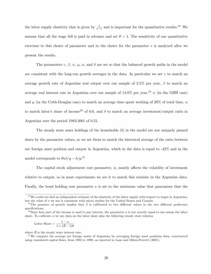
the labor supply elasticity that is given by 1ν−1 and is important for the quantitative results.

18 We

assume that all the wage bill is paid in advance and set θ = 1. The sensitivity of our quantitative

exercises to this choice of parameter and to the choice for the parameter v is analyzed after we

present the results.

The parameters γ, β, ψ, µ, α, and δ are set so that the balanced growth paths in the model

are consistent with the long-run growth averages in the data. In particular we set γ to match an

average growth rate of Argentine real output over our sample of 2.5% per year, β to match an

average real interest rate in Argentina over our sample of 14.8% per year,19 ψ (in the GHH case)

and µ (in the Cobb-Douglas case) to match an average time spent working of 20% of total time, α

to match labor’s share of income20 of 0.6, and δ to match an average investment/output ratio in

Argentina over the period 1983-2001 of 0.21.

The steady state asset holdings of the households (b) in the model are not uniquely pinned

down by the parameter values, so we set them to match the historical average of the ratio between

net foreign asset position and output in Argentina, which in the data is equal to -42% and in the

model corresponds to θwl/y − b/y.21

The capital stock adjustment cost parameter, φ, mostly affects the volatility of investment

relative to output, so in most experiments we set it to match this statistic in the Argentine data.

Finally, the bond holding cost parameter κ is set to the minimum value that guarantees that the

18We could not find an independent estimate of the elasticity of the labor supply with respect to wages in Argentina,but the value of v we use is consistent with micro studies for the United States and Canada.19The presence of growth implies that β is calibrated to two different values in the two different preference

specifications.20Since here part of the income is used to pay interest, the parameter α is not exactly equal to one minus the labor

share. To calibrate α we use data on the labor share plus the following steady state relation

Labor Share =1− α

1 + (R− 1)θ

where R is the steady state interest rate.21We compute the average net foreign assets of Argentina by averaging foreign asset positions data, constructed

using cumulated capital flows, from 1983 to 1998, as reported in Lane and Milesi-Ferretti (2001).

20

equilibrium solution is stationary. The parameter values are summarized in Table 2. Once shock

processes and parameters are set, it is straightforward to compute impulse responses to shocks and

simulation results based on equilibrium paths of the economy, computed by log-linearizing the model

around its balanced growth path.

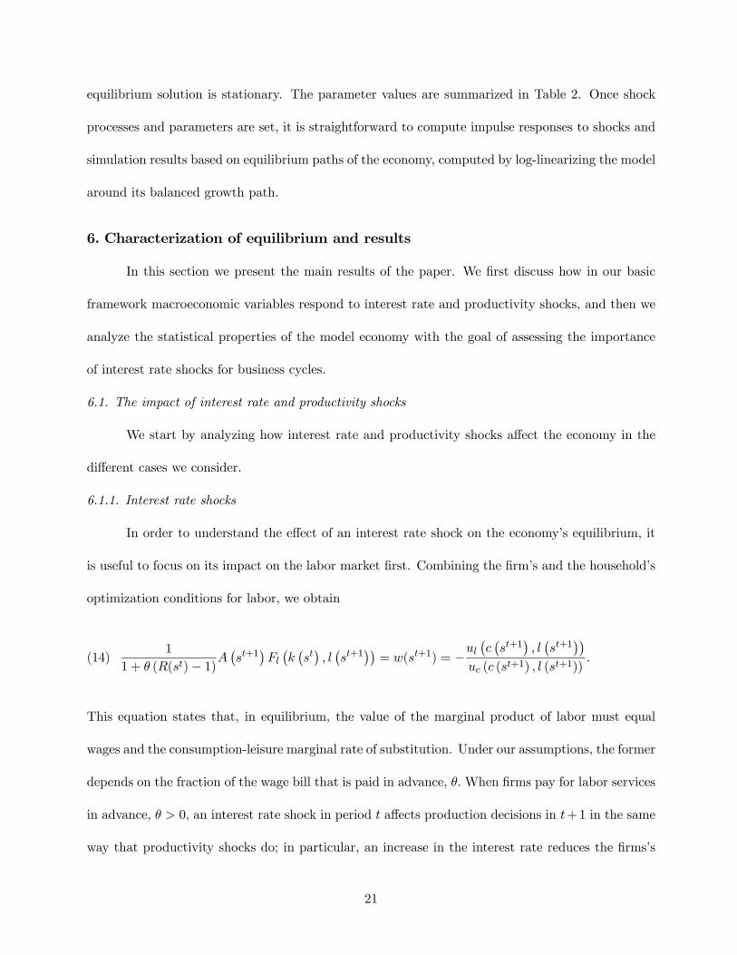
6. Characterization of equilibrium and results

In this section we present the main results of the paper. We first discuss how in our basic

framework macroeconomic variables respond to interest rate and productivity shocks, and then we

analyze the statistical properties of the model economy with the goal of assessing the importance

of interest rate shocks for business cycles.

6.1. The impact of interest rate and productivity shocks

We start by analyzing how interest rate and productivity shocks affect the economy in the

different cases we consider.

6.1.1. Interest rate shocks

In order to understand the effect of an interest rate shock on the economy’s equilibrium, it

is useful to focus on its impact on the labor market first. Combining the firm’s and the household’s

optimization conditions for labor, we obtain

(14)1

1 + θ (R(st)− 1)A¡st+1

¢Fl¡k¡st¢, l¡st+1

¢¢= w(st+1) = −

ul¡c¡st+1

¢, l¡st+1

¢¢uc (c (st+1) , l (st+1))

.

This equation states that, in equilibrium, the value of the marginal product of labor must equal

wages and the consumption-leisure marginal rate of substitution. Under our assumptions, the former

depends on the fraction of the wage bill that is paid in advance, θ.When firms pay for labor services

in advance, θ > 0, an interest rate shock in period t affects production decisions in t+1 in the same

way that productivity shocks do; in particular, an increase in the interest rate reduces the firms’s

21

demand for labor for any level of wages.

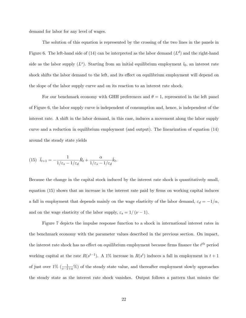
The solution of this equation is represented by the crossing of the two lines in the panels in

Figure 6. The left-hand side of (14) can be interpreted as the labor demand (Ld) and the right-hand

side as the labor supply (Ls). Starting from an initial equilibrium employment l0, an interest rate

shock shifts the labor demand to the left, and its effect on equilibrium employment will depend on

the slope of the labor supply curve and on its reaction to an interest rate shock.

For our benchmark economy with GHH preferences and θ = 1, represented in the left panel

of Figure 6, the labor supply curve is independent of consumption and, hence, is independent of the

interest rate. A shift in the labor demand, in this case, induces a movement along the labor supply

curve and a reduction in equilibrium employment (and output). The linearization of equation (14)

around the steady state yields

(15) lt+1 = −1

1/εs − 1/εdRt +

α

1/εs − 1/εdkt.

Because the change in the capital stock induced by the interest rate shock is quantitatively small,

equation (15) shows that an increase in the interest rate paid by firms on working capital induces

a fall in employment that depends mainly on the wage elasticity of the labor demand, εd = −1/α,

and on the wage elasticity of the labor supply, εs = 1/ (ν − 1).

Figure 7 depicts the impulse response function to a shock in international interest rates in

the benchmark economy with the parameter values described in the previous section. On impact,

the interest rate shock has no effect on equilibrium employment because firms finance the tth period

working capital at the rate R(st−1). A 1% increase in R(st) induces a fall in employment in t + 1

of just over 1% ( 1v−1+α%) of the steady state value, and thereafter employment slowly approaches

the steady state as the interest rate shock vanishes. Output follows a pattern that mimics the

22

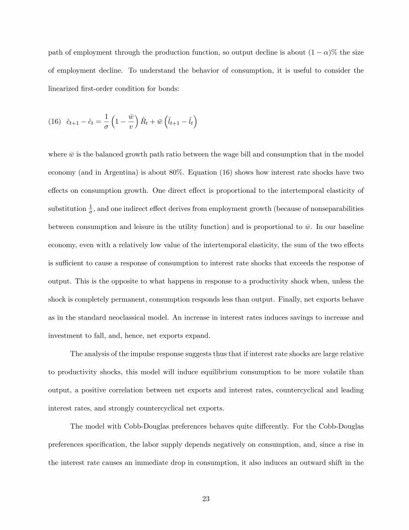
path of employment through the production function, so output decline is about (1− α)% the size

of employment decline. To understand the behavior of consumption, it is useful to consider the

linearized first-order condition for bonds:

(16) ct+1 − ct =1

σ

³1− w

v

´Rt + w

³lt+1 − lt

´

where w is the balanced growth path ratio between the wage bill and consumption that in the model

economy (and in Argentina) is about 80%. Equation (16) shows how interest rate shocks have two

effects on consumption growth. One direct effect is proportional to the intertemporal elasticity of

substitution 1σ , and one indirect effect derives from employment growth (because of nonseparabilities

between consumption and leisure in the utility function) and is proportional to w. In our baseline

economy, even with a relatively low value of the intertemporal elasticity, the sum of the two effects

is sufficient to cause a response of consumption to interest rate shocks that exceeds the response of

output. This is the opposite to what happens in response to a productivity shock when, unless the

shock is completely permanent, consumption responds less than output. Finally, net exports behave

as in the standard neoclassical model. An increase in interest rates induces savings to increase and

investment to fall, and, hence, net exports expand.

The analysis of the impulse response suggests thus that if interest rate shocks are large relative

to productivity shocks, this model will induce equilibrium consumption to be more volatile than

output, a positive correlation between net exports and interest rates, countercyclical and leading

interest rates, and strongly countercyclical net exports.

The model with Cobb-Douglas preferences behaves quite differently. For the Cobb-Douglas

preferences specification, the labor supply depends negatively on consumption, and, since a rise in

the interest rate causes an immediate drop in consumption, it also induces an outward shift in the

23

labor supply curve. Since on impact the labor demand does not move, an interest rate shock will

cause employment and output, on impact, to go up. In subsequent periods the interest rate shock

shifts the labor demand to the left; this can offset the outward shift in the labor supply curve,

and the final effect on equilibrium employment can be positive or negative (see the right panel of

Figure 6). Analytically, the linearized version of the labor market equilibrium condition, (14), under

Cobb-Douglas preferences becomes

(17) lt+1 = −1

l1−l − 1/εd

³Rt + ct+1

´+

αl1−l − 1/εd

kt

where l is the constant value of employment along the balanced growth path. Since kt is small the

effect of Rt on lt+1 depends on the consumption response relative to Rt. If consumption responds

strongly to interest rates, labor supply will increase a lot and employment will tend to increase even

in subsequent periods. If consumption does not move much, labor supply will be more stable and

employment will fall. In the sensitivity section we will discuss the key parameters that affect the

magnitude of these effects.

6.1.2. Productivity shocks

The effect of productivity shocks on the economy will depend on the nature of country

risk. In the case in which country risk is independent of these shocks, the reaction of the econ-

omy to a productivity shock is the same as in the standard business cycle model of a small open

economy (see, for example, Mendoza, 1991). A shock to total factor productivity increases the

labor demand for any level of wages and induces a change in equilibrium employment that depends

on the wage elasticities of the labor supply and demand, εs and εd. The change in employment

is lt+j = 1/ (1/εs − 1/εd) At+j , where the autoregressive process for At specified in (8) implies

At+j = ρjA εAt for j = 0, 1, . . . .

24

In the case in which country risk is “induced” by productivity shocks as in (7), changes in

country risk act as an amplification mechanism of fluctuations in productivity through the working

capital channel. The best way of illustrating this is by analyzing the effect of productivity shocks

on equilibrium employment, shown in the following equation:

lt =1

1/εs − 1/εdεAt(18a)

lt+j =1

1/εs − 1/εd

Ã1 +

Rθ

1 +¡R− 1

¢θη ρ−1A

!ρjAεAt for j = 1, 2, . . . .(18b)

On impact a productivity shock has the same effect as in the standard neoclassical model

as shown in (18a). In this model, in addition, a positive productivity shock reduces country risk,

following (7), and this affects the labor demand in all future periods as shown in (18b). When

country spreads are a function of productivity shocks, the rise in productivity induces a fall in

interest rates which, in turn, further expands the labor demand for any level of wages. The size of

this amplification effect of productivity shocks on the labor demand is equal to the term in brackets

in equation (18b), and it depends on the sensitivity of interest rates to productivity shocks, η, and on

the proportion of the wage bill that has to be financed in advance, θ. Thus, the interaction between

the effect of productivity shocks on country risk and the assumption of working capital amplifies

the effect of a productivity shock. If there is no spillover effect from productivity shocks to country

risk, η = 0, or if there is no need for working capital, θ = 0, the amplification effect disappears,

and the model behaves as a standard business cycle model. Under our parameter specification with

η = 1.04, for θ = 1, the impact of a productivity shock in t on employment in t+ j, for j ≥ 1, more

than doubles its size relative to the standard model.

6.2. Computational experiments

In order to assess the role of interest rates in driving business cycles, we now analyze the

25

statistical properties of the model economy using three experiments. First, we consider a model

economy without country risk, then we analyze the model economy with independent country risk,

and finally, we analyze the economy with induced country risk. In all three experiments we will

include shocks to international interest rates R∗ and consider the benchmark model with working

capital, θ = 1, and GHH preferences. Table 3 and Figures 8 and 9 contain the results. Finally,

we discuss how some of the key effects analyzed here change when we deviate from the baseline

parameterization.

6.2.1. No country risk

In the first experiment we analyze business cycle statistics in a model economy where the

only shocks are to international interest rates R∗ (U.S. real yield on non-investment-grade bonds)

and then consider an economy with shocks to international rates and to TFP. To generate interest

rates in the model, we use (9) and the innovations from the data to mimic the actual behavior of

the percentage deviations from trend of R∗. Productivity shocks are randomly generated by (8),

and the standard deviation of productivity innovations, σ(εA¡st¢), is set so that the volatility of

GDP in the model with both shocks exactly matches the volatility of GDP in Argentina. The

capital adjustment cost parameter, φ, is set so that the model with both shocks matches the relative

volatility of investment in the data.

The model with only interest rate shocks (lines (a) in Table 3) generates a GDP volatility

of 1.24% that is about 30% of the volatility of GDP in the data. Notice though that once we add

TFP shocks, so that GDP volatility in the model is in line with GDP volatility in the data, the

cross-correlation between interest rates and GDP in the model without country risk is quite far

from the cross-correlation in the data (Figure 8): in particular, interest rates in the model are much

less countercyclical than in the data. Also, the model is not able to generate countercyclical net

exports or consumption that is more volatile than output (lines (b) in Table 3). We conclude that

26

the absence of country risk prevents the model from explaining important features of the data.

6.2.2. Independent country risk

Lines (c) in Table 3 report statistics for the economy subject to shocks to international real

interest rates and to independent country risk, while lines (d) report the statistics for the same

economy also subject to TFP shocks. To generate international real interest rates and country risk

in the model, we use (9) and (10) plus the innovations from the data so that the series for the

percentage deviations from trend of interest rates in the model, Rt and R∗t , are identical to the

series in the data. As in the preceding experiment, TFP shocks are randomly generated by (8).

The standard deviation of productivity innovations, σ(εA¡st¢), and the capital adjustment cost

parameter, φ, are set so that the volatility of GDP and the relative volatility of investment in the

model with all three shocks exactly match the data.

Figure 9 shows the path for detrended output predicted by the model with only international

interest rates and country risk shocks against detrended output in the data.

The series for output predicted by the model displays cyclical fluctuations very similar to

the data, with a correlation between the actual and the simulated output series of 0.73. The figure

suggests that country risk fluctuations can be a key factor in explaining business cycle volatility

in emerging economies. In lines (c) in the first panel of Table 3, we can see that the volatility of

output in the model is 2.33, or 55% of that in the data. Lines (c) though also show that the model

with only interest rate shocks exaggerates the relative volatility of consumption, employment, and

investment, as well as the correlation between interest rates and the main macroeconomic variables,

thus suggesting the importance of other shocks. Indeed, the model with productivity shocks matches

the data better along a number of dimensions. Figure 8 shows that the cross-correlation between

GDP and interest rates generated by this model (the line with triangular markers) is quite close

to the data. The model can also generate consumption that is more volatile than output (lines (d)

27

in the first panel), countercyclical net exports (lines (d) in the second panel), and comovements

between interest rates and macroeconomic aggregates that are close to the data.

Still some discrepancies between the model and the data remain. In particular, the negative

comovement between interest rates and output in the model (-0.29) is about half of what it is in the

data (-0.63), and net exports are much less countercyclical than in the data (-0.08 vs. -0.89). These

discrepancies might be due to the fact that, in the current experiment, country risk affects business

cycles but business cycles do not affect country risk. If, as we do in the next experiment, we also

allow business cycles to influence country risk, the negative comovement between business cycles

and interest rates will increase. Also, since, as we discussed previously, interest rate increases tend

to generate a net exports boom, a negative impact of business cycles on interest rates will generate

more countercyclical net exports.

6.2.3. Induced country risk

In this final experiment we study the effect of allowing productivity shocks to determine

country risk. As in previous experiments, shocks to international interest rates R∗ are determined

by (9), but country risk is now induced by TFP shocks according to (11) so that the series for

interest rates generated by the model has the same standard deviation and persistence as in the data.

TFP shocks are randomly generated by (8). The standard deviation of productivity innovations,

σ(εA¡st¢), and the capital adjustment cost parameter, φ, are set so that the volatility of GDP

and the relative volatility of investment in the model exactly match the data. Observe that with

this specification the model is able to reproduce well the entire U-shaped dynamic structure of

cross-correlations between output and interest rates observed in the data (in Figure 8 compare the

line with the square markers with the line without markers) and the comovements of the main

macroeconomic aggregates with output and interest rates (lines (e) in the second and third panels

of Table 3), including the countercyclicality of net exports. Two discrepancies between the model

28

and the data remain: the model overpredicts the relative volatility of employment and the relative

volatility of consumption and net exports. Regarding employment volatility, as we discussed in

the data section, we have reasons to suspect that the volatility of employment in Argentine data

underestimates the true volatility of labor input, so the part of the difference between model and

data might reflect this issue. The excess volatility of net exports and consumption instead arises

because, in the model, the household sector is directly facing the volatile rate R(st). In response to

large fluctuations in R(st), households intertemporally substitute their consumption decision and

this leads to high consumption volatility and high net exports volatility. Reducing the willingness

of households to substitute is a possible way of bringing the model in line with the data.22

Since this last setup can account well for most of the Argentine data, we can use it to

quantify the contribution of interest rate shocks to business cycle volatility. That is, we can ask how

much GDP volatility would decline if one could eliminate fluctuations in international real rates

or fluctuations in country risk. To estimate the contribution of international real rate fluctuations,

we simply recompute the equilibrium without shocks to the international real rates. We find that

the percentage standard deviation of GDP in the model without shocks to international rates is

4.10, only 3% smaller than the percentage standard deviation of GDP in the model with all shocks

(4.22).23

To estimate the contribution of country risk fluctuations, we recompute the model setting

η = 0 and σ(εI) = 0 so that country risk is absent from the model. In particular, when η = 0 the

22We experimented with increasing the parameter σ from 5 to 10, and the change brought both the volatility ofconsumption and the volatility of net exports in line with the data without significantly changing the other statisticsgenerated by the model. Detailed results of this experiment are available upon request.23The reason the volatility reduction from eliminating shocks to international rates is so small is that their variance

is small compared to the variance of country risk. When international rates are eliminated, the standard deviation ofthe real interest rate falls but only from 3.87% to 3.67%. Since equation (15), together with the linearized productionfunction, tells us that, approximately, the standard deviation of GDP is proportionally equal to 1−α

v−1−α=0.63 timesthe volatility of R, a reduction of 20 points in the volatility of R only leads to a reduction in the volatility of GDP ofaround 12/13 points, that is, around 3% of the volatility in the data. If country risk were not present, then eliminatingthe shocks to international rates would have a larger impact on GDP volatility.

29

amplification of productivity shocks created by country risk (see equation (18)) disappears. In this

case the percentage standard deviation of output drops to 3.06, more than 27% below the volatility

of the model with all shocks.

The main lesson we learn from these three experiments is that in emerging economies the large

fluctuations in country risk seem to be deeply connected with the large fluctuations in economic

activity. The model that better reproduces the data is the one in which country risk is affected

by fundamentals (through equation (11)) and at the same time, through the presence of working

capital, amplifies the effects of fundamental shocks on the economy. Both directions of causation

seem to be quantitatively important, and both deserve further investigation.

6.2.4. Sensitivity analysis

The elements of the model that are crucial for determining the effects of interest rate fluctu-

ations on business cycles are the type of utility function, the elasticity of labor supply in the GHH

preferences, and the presence of working capital. In Table 4 we analyze how the size of these effects

quantitatively depends on these elements. In the table we report two key statistics from the model,

the volatility of output (relative to the volatility of output in the data) and the correlation of output

with interest rates for a variety of parameter configurations. We consider a high and a low value of

the labor supply elasticity24 in the GHH preferences and the case of Cobb-Douglas preferences with

a high and low value of the parameter σ, which determines the intertemporal elasticity of substitu-

tion. We also consider a case in which only 50% of the labor cost has to be paid in advance (θ = 0.5)

and a case in which it is not necessary to pay labor in advance (θ = 0). In all the cases we keep all

parameters constant to their baseline value, and since we want to quantify the effect of interest rate

shocks on business cycles, we focus on the model with only interest rate shocks (international real

rates and independent country risk).

24A value of v = 1.2 implies an elasticity of five, while v = 4 implies an elasticity of one-third.

30

First, focus on the baseline GHH preferences. When θ = 1 (100% of labor costs have to be

paid in advance) the model generates a quite volatile output and a negative correlation between

output and interest rates. Note that as we reduce the working capital parameter θ from one to zero,

both the volatility of output and the absolute value of the (negative) correlation between output

and interest rates are reduced. This is because by reducing θ we reduce the negative impact that

interest rates have on labor demand. Notice though that even with θ = 0.5 interest rate shocks

induce significant output fluctuations (about one-third of the one observed in the data) that are

negatively correlated with interest rates. When we set θ = 0 (no working capital), the model

reduces to the one in Mendoza (1991). In this case interest rates generate relatively small output

fluctuations that are also positively correlated with interest rates, so it has no hope of explaining

emerging economies data.25

Now consider changes in the labor supply elasticity in the GHH preferences. For a fixed θ

(that determines how labor demand responds to interest rate shocks) increasing the labor supply

elasticity (in terms of Figure 6, making the Ls curve flatter) generates larger output fluctuations

and decreasing it induces smaller output fluctuations; for all values of v the correlation between

output and interest rates is negative as long as interest rates affect labor demand (θ > 0).

The importance of the specification of preferences is considered in the last four columns of

Table 4 in which we analyze how the model behaves with Cobb-Douglas preferences. The intuition

underlying the reaction of the economy to interest rate shocks in this case is discussed in Section

6. In the model with Cobb-Douglas preferences and with σ = 5, interest rate shocks can generate

substantial output volatility, but interest rate shocks are highly positively correlated with output.

As discussed previously the positive correlation between output and interest rates arises because

25The positive correlation between output and interest rates in this case can be understood in terms of the responseto an interest rate innovation. On impact output does not move, but in the subsequent period, investment falls andoutput slowly declines because of the fall in capital stock. Interest rates also slowly decline, reverting to their steadystate levels. This contemporaneous decline gives rise to (mildly) positive comovement between the two variables.

31

the change in consumption induced by the interest rate shock increases the labor supply, offsetting

the effect of interest rates on the labor demand as shown in (17). As we reduce θ both the output-

interest rate correlation and the volatility of output increase. To understand this consider the right

panel of Figure 6: in response to interest rate shocks the consumption effect shifts labor supply to

the right while the working capital effect shifts the labor demand to the left. If θ = 1 the two effects

tend to offset each other, dampening the fluctuations in equilibrium employment. As we reduce

θ the consumption effect dominates and it causes equilibrium employment and output to increase

more in response to an increase in interest rates.

Because the change in consumption mentioned above depends on the intertemporal elasticity

of substitution, 1/σ, a low value of 1/σ can, by dampening the labor supply response, induce a

negative comovement between interest rates and output even in the Cobb-Douglas case. The last

two columns confirm that is indeed the case. When σ = 50 consumption does not move much

in response to interest rate shocks and consequently labor supply increases very little. If θ = 1

labor demand declines significantly, and thus the increase in the interest rate leads to reductions in

employment and output. This is to show that GHH utility is not essential to generate a negative

impact of interest rate shocks on output.26

7. Conclusions

The fundamental issue addressed in this paper is why business cycles in emerging economies

are much more pronounced than in developed economies. In particular, we explore the role of

fluctuations in the real interest rates faced by these economies. We started by documenting some

features of business cycles in a group of five emerging economies. Beyond the high volatility, these

countries are also characterized by consumption volatility higher than output volatility and strongly

26The overall performance of a model with a Cobb-Douglas production function and σ = 50 is comparable to themodel with GHH preferences. Complete results are not reported for brevity, but are available upon request.

32

countercyclical net exports. We also find that in these five economies real interest rates are quite

volatile, strongly countercyclical and they lead the cycle.

We experiment with two ways of modeling the interest rate: one as a process completely

independent from the fundamental shocks hitting the economy and the other as a process that is

largely induced by these shocks. We find that adding the latter way of modeling interest rates

to a simple dynamic general equilibrium model of a small open economy can explain the facts

well. Real interest rates are induced by fundamental shocks but also, through the presence of

working capital, amplify the effect of fundamental shocks on business cycles, contributing to the

high volatility. We then use this model to evaluate the impact on business cycles of real interest rate

fluctuations induced by fundamentals. We find that eliminating default risk in emerging economies

can reduce about 27% of their output volatility. This finding suggests the importance of studying

further both the mechanism through which fundamental shocks induce interest rate fluctuations and

the mechanism through which interest rate fluctuations amplify the effects of fundamental shocks.

Understanding these mechanisms could be key to designing policies or reforms that help stabilize

emerging economies.

33

Data Appendix

1. Developed countries

1.1. National accounts

For all countries quarterly series for constant prices GDP, private consumption, total con-

sumption (private and government consumption plus statistical discrepancy and change in inven-

tories), gross fixed capital formation, and exports and imports of goods and services are obtained

from OECD Quarterly National Accounts (QNA).

1.2. Employment and hours

For all countries except Netherlands, the quarterly employment series is the civilian employ-

ment index from OECD MEI. For Netherlands it is the number of jobs by employees from OECD

Main Economic Indicators (MEI).

Total hours is obtained as the employment series multiplied by weekly hours of work. For

Australia and Canada we use weekly hours of work in manufacturing from OECD MEI. For New

Zealand we use weekly hours of work in nonagricultural establishments from ILO LABSTAT data

set. For Sweden we use weekly hours worked in industry (OECD MEI) from 1987.1. From 1980.1 to

1986.4 we use weekly hours per person from ILO LABSTAT. The two series are joined by rescaling

the ILO series so that the 1987.1 series has the same value as the OECD series. For Netherlands a

consistent series of weekly hours worked is not available.

1.3. Real interest rates

For Australia and Canada the nominal interest rate series we use is the 90-day corporate

commercial paper from OECD MEI. For Netherlands from 1983.3 to 1985.4, we use the call money

rate, and from 1986.1 to 2001.4, we use the 90-day BAIBOR. When the two series overlap, their

differences are negligible. Data are obtained from the Bank of Netherlands. For New Zealand the

interest rate is the 90-day bank bill from OECD MEI. For Sweden it is the rate on 90-day treasuries

34

from OECD MEI.

For all countries the real rate is obtained by subtracting the expected GDP deflator inflation

from the nominal rate. Expected inflation in period t is computed as the average of inflation in the

current period and in the three preceding periods.

2. Emerging countries

2.1. National accounts

For Argentina all series are in constant prices from Ministerio de Economía (MECON). The

series for private consumption is only available from 1993.1. For Brazil all series are from Instituto

Brasileiro de Geografia e Estatística (IBGE), Novo Sistema de Contas Nacionais. Real variables are

obtained by dividing nominal components of GDP by the GDP deflator. For Mexico and Korea all

series in constant prices are from OECD QNA. For Philippines all series are from IMF International

Financial Statistics. Real variables are obtained by dividing nominal components of GDP by the

GDP deflator.

2.2. Employment and hours

For Argentina the series for employment is the number of employed people working at least

35 hours per week and the series for total hours is employment multiplied by the average weekly

hours worked in Buenos Aires (both series are from Encuesta Permanente de Hogares, Table A3.2,

Informe Economico). Both series are semiannual, and the series for hours is only available from

1986.2.

For Brazil employment is the number of employed persons in urban areas from IBGE Pesquisa

Mensal de Emprego. Total hours are computed as employment times hours per person. Hours

per person are computed by dividing the index of total hours worked in manufacturing by the

employment index in manufacturing. Both indexes are from Confederação Nacional da Indústria,

Indicadores Industriais. For Korea employment is civilian employment from OECD MEI. Total

35

hours are employment times weekly hours of work. Weekly hours are from ILO LABSTAT (until

1998), and from 1999 to 2001 they are weekly hours of work (annual series) from the Korean National

Statistical Office.

For Mexico employment is derived as (1-unemployment rate) × (rate of activity of population

over 12 years of age) × (fraction of population over 12 years of age) × total population. All series are

from Instituto Nacional de Estatistica Geografia e Informatica except total population, which is from

World Bank World Development Indicators. Total hours are computed as employment times hours

per person. Hours per person are obtained by dividing the total hours of work in manufacturing

(OECD MEI) by the employment in manufacturing (OECD MEI).

For Philippines employment is from ILO LABSTAT data set. A consistent series of weekly

hours worked is not available.

2.3. Real interest rates

For all countries nominal interest rate in dollars for the period 1994.1-2001.4 are constructed

as the 90-day U.S. T-bill rate plus the J.P. Morgan EMBI Global Spread.27 Real rates are obtained

by subtracting expected U.S. GDP deflator inflation from the nominal dollar rate. Expected inflation

in period t is computed as the average of inflation in the current period and in the three preceding

periods.

For Argentina we were able to extend the series of dollar denominated interest rates by

constructing, using a procedure developed by Alvarez et al. (1999), an interest rate series starting

in the second quarter of 1983. We use data on prices of Argentine government dollar denominated

bonds (BONEX 80, BONEX 81, BONEX 82, BONEX 84, BONEX 89, GRA, Brady Discount,

Global 01, Global 03, Global 06, Global 17, Global 27) and U.S. treasury strips. The Argentine rate

on a j period zero coupon bond in period t, rargt,j , can be written as the sum of the U.S. rate for a

27The data for Brazil start in 1994.3.

36

similar bond, rUSt,j , plus a country spread, δt,j . To estimate the term spreads, δt,j , we assume they

are given by the following functional form (a polynomial on j and t)

δt,j = δ(t, j) + εt,j = ∆t + α1(t) · j + α2(t) · j2 + α3(t) · j3 + εt,j(19)

where αi(t) = ai,0 + ai,1 · t+ ai,2 · t2 + ai,3 · t3, i = 1, 2, 3

εt,j is the approximation error, and ∆t is a fixed effect for each period (that can be interpreted as

the spread of a zero maturity bond). The price, at period t, of a coupon bond, k, issued by the

Argentine government, P argk,t , is given by

P argk,t =JX

j=1

Ck,j · exp(−(rust,j + δt,j) · j)

where Ck,j is the coupon paying at t of bond k. The estimated parameters, ai,.and ∆t, of the spread

function (19) are those that minimize the loss function L, that is,

minai,.∆t

L =TXt=1

KXk=1

⎡⎣ 1

durt,kln

⎛⎝PJj=1 cj · exp

³−³rust,j + δ (t, j)

´· j´

P argk,t

⎞⎠⎤⎦2

where durt,k is the duration of bond k at time t, which is given by

durt,k =

PJj=1 ckj · exp

³−rust,j · j

´jPJ

j=1 ckj · exp³−rust,j · j

´ .

Thus, the series for 3-month Argentine nominal dollar interest rates from 1983.2 until 1993.4 is the

sum of the U.S. 3-month treasury bill interest rate and the estimated spread with j = 3. For the

period 1994.1-2000.1, we can compare the series for the Argentine rate constructed by us with the

series constructed using the EMBI, and the two series have similar levels and comove very closely.

37

References

[1] Agénor, P.-R., J.C. McDermott and E.S. Prasad, 2000, Macroeconomic fluctuations in devel-

oping countries: Some stylized facts, World Bank Economic Review 14 (2), 251-285.

[2] Alvarez, F., F. Buera and P. Neumeyer, 1999, Fitting a sovereign spread curve in an economy

with incomplete markets. Manuscript, Universidad T. di Tella.

[3] Arellano, C., 2003, Default risk, the real exchange rate and income fluctuations in emerging

economies. Manuscript, Duke University.

[4] Backus, D.K. and P.J. Kehoe, 1992, International evidence on the historical properties of

business cycles, American Economic Review 82 (4), 864-888.

[5] Benhabib, J., R. Rogerson and R. Wright, 1991, Homework in macroeconomics: household

production and aggregate fluctuations, Journal of Political Economy 99 (6), 1166-1187.

[6] Calvo, G.A., 1998, Capital flows and capital-market crises: The simple economics of sudden

stops, Journal of Applied Economics 1 (1), 35-54.

[7] Calvo, G.A. and C.A. Vegh, 1999, Inflation stabilization and BOP crises in developing countries,

in: J. Taylor and M. Woodford, eds., Handbook of macroeconomics, Vol. C (North-Holland,

Amsterdam) 1531-1614.

[8] Christiano, L.J. and M. Eichenbaum, 1992, Liquidity effects and the monetary transmission

mechanism, American Economic Review 82 (2), 346-353.

[9] Christiano, L.J., C. Gust and J. Roldos, 2003, Monetary policy in a financial crisis, Journal of

Economic Theory, forthcoming.

[10] Cooley, T.F. and G.D. Hansen, 1989, The inflation tax in a real business cycle model, American

Economic Review 79 (4), 733-748.

38

[11] Correia, I., J.C. Neves, and S. Rebelo, 1995, Business cycles in a small open economy, European

Economic Review 39 (6), 1089-1113.

[12] Eaton, J., and M. Gersovitz, 1981, Debt with potential repudiation: Theoretical and empirical

analysis, Review of Economic Studies 48 (2), 289-309.

[13] Greenwood, J., Z. Hercovitz, and G.W. Huffman, 1988, Investment, capacity utilization, and

the real business cycle. American Economic Review 78 (3), 402-417.

[14] Kehoe, P.J., and F. Perri, 2004, Competitive equilibria with limited enforcement, Journal of

Economic Theory, forthcoming.

[15] Kydland, F.E. and C.E.J.M. Zarazaga, 1997, Is the business cycle of Argentina “different”?

Federal Reserve Bank of Dallas Economic Review, 4th Quarter, 21-36.

[16] Kydland, F.E. and C.E.J.M. Zarazaga, 2002, Argentina’s lost decade, Review of Economic

Dynamics 5 (1), 152-165.

[17] Lane, P.R. and G.M. Milesi-Ferretti, 2001, The external wealth of nations: measures of foreign

assets and liabilities for industrial and developing countries, Journal of International Economics

55 (2), 263-294.

[18] Mendoza, E.G., 1991, Real business cycles in a small open economy, American Economic Review

81 (4), 797-818.

[19] Mendoza E.G., 1995, The terms of trade, the real exchange rate, and economic fluctuations,

International Economic Review 36 (1), 101-137.

[20] Mendoza E.G. and K.A. Smith, 2002, Margin calls, trading costs, and asset process in emerging

markets: The financial mechanics of the ‘sudden stop’ phenomenon, NBER Working Paper

9286.

39

[21] Neumeyer, P.A., 1999, Inflation-stabilization risk in economies with incomplete asset markets,

Journal of Economic Dynamics and Control 23 (3), 371-391.

[22] Prasad, E., K. Rogoff, S.J. Wei and M.A. Kose, 2003, Effects of financial globalization on

developing countries: Some empirical evidence. Manuscript, International Monetary Fund.

[23] Rebelo, S. and C.A. Vegh, 1995, Real effects of exchange-rate-based stabilization: An analysis of

competing theories, in: B.S. Bernanke and J. Rotemberg, eds., NBER macroeconomics annual

1995 (MIT Press, Cambridge, MA) 125-174.

[24] Reinhart, C.M. and C.A. Vegh, 1995, Nominal interest rates, consumption booms, and lack of

credibility: A quantitative examination, Journal of Development Economics 46 (2) 357-378.

[25] Schmitt-Grohé, S., and M. Uribe, 2003, Closing small open economy models, Journal of Inter-

national Economics 61 (1), 163-185.

[26] Uribe, M., 1997, Exchange-rate-based inflation stabilization: The initial real effects of credible

plans, Journal of Monetary Economics 39 (2), 197-221.

[27] Uribe, M. and V.Z. Yue (2003), Country spreads and emerging countries: Who drives whom?

NBER Working Paper 10018.

40

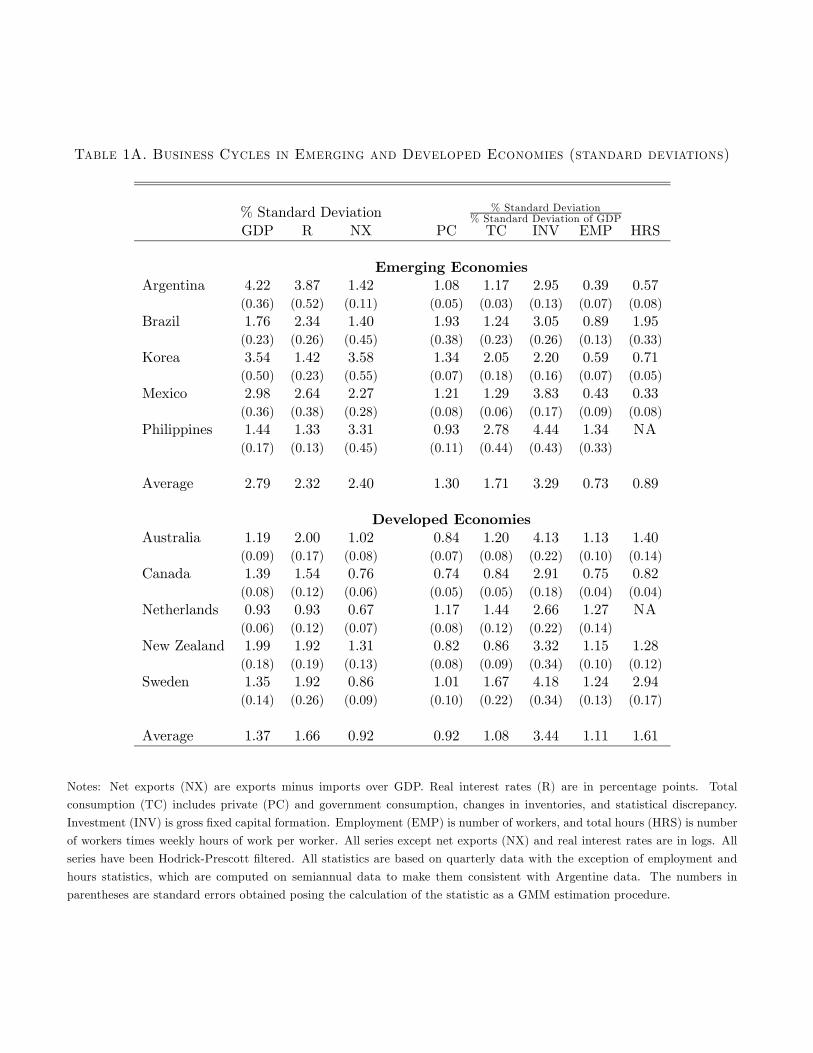
Table 1A. Business Cycles in Emerging and Developed Economies (standard deviations)

% Standard Deviation % Standard Deviation% Standard Deviation of GDP

GDP R NX PC TC INV EMP HRS

Emerging EconomiesArgentina 4.22 3.87 1.42 1.08 1.17 2.95 0.39 0.57

(0.36) (0.52) (0.11) (0.05) (0.03) (0.13) (0.07) (0.08)Brazil 1.76 2.34 1.40 1.93 1.24 3.05 0.89 1.95

(0.23) (0.26) (0.45) (0.38) (0.23) (0.26) (0.13) (0.33)Korea 3.54 1.42 3.58 1.34 2.05 2.20 0.59 0.71

(0.50) (0.23) (0.55) (0.07) (0.18) (0.16) (0.07) (0.05)Mexico 2.98 2.64 2.27 1.21 1.29 3.83 0.43 0.33

(0.36) (0.38) (0.28) (0.08) (0.06) (0.17) (0.09) (0.08)Philippines 1.44 1.33 3.31 0.93 2.78 4.44 1.34 NA

(0.17) (0.13) (0.45) (0.11) (0.44) (0.43) (0.33)

Average 2.79 2.32 2.40 1.30 1.71 3.29 0.73 0.89

Developed EconomiesAustralia 1.19 2.00 1.02 0.84 1.20 4.13 1.13 1.40

(0.09) (0.17) (0.08) (0.07) (0.08) (0.22) (0.10) (0.14)Canada 1.39 1.54 0.76 0.74 0.84 2.91 0.75 0.82

(0.08) (0.12) (0.06) (0.05) (0.05) (0.18) (0.04) (0.04)Netherlands 0.93 0.93 0.67 1.17 1.44 2.66 1.27 NA

(0.06) (0.12) (0.07) (0.08) (0.12) (0.22) (0.14)New Zealand 1.99 1.92 1.31 0.82 0.86 3.32 1.15 1.28

(0.18) (0.19) (0.13) (0.08) (0.09) (0.34) (0.10) (0.12)Sweden 1.35 1.92 0.86 1.01 1.67 4.18 1.24 2.94

(0.14) (0.26) (0.09) (0.10) (0.22) (0.34) (0.13) (0.17)

Average 1.37 1.66 0.92 0.92 1.08 3.44 1.11 1.61

Notes: Net exports (NX) are exports minus imports over GDP. Real interest rates (R) are in percentage points. Total

consumption (TC) includes private (PC) and government consumption, changes in inventories, and statistical discrepancy.

Investment (INV) is gross fixed capital formation. Employment (EMP) is number of workers, and total hours (HRS) is number

of workers times weekly hours of work per worker. All series except net exports (NX) and real interest rates are in logs. All

series have been Hodrick-Prescott filtered. All statistics are based on quarterly data with the exception of employment and

hours statistics, which are computed on semiannual data to make them consistent with Argentine data. The numbers in

parentheses are standard errors obtained posing the calculation of the statistic as a GMM estimation procedure.

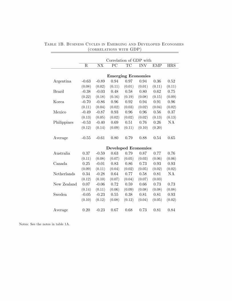
Table 1B. Business Cycles in Emerging and Developed Economies(correlations with GDP)

Correlation of GDP withR NX PC TC INV EMP HRS

Emerging EconomiesArgentina -0.63 -0.89 0.94 0.97 0.94 0.36 0.52

(0.08) (0.02) (0.11) (0.01) (0.01) (0.11) (0.11)Brazil -0.38 -0.03 0.48 0.58 0.80 0.62 0.75

(0.22) (0.18) (0.16) (0.19) (0.08) (0.15) (0.09)Korea -0.70 -0.86 0.96 0.92 0.94 0.91 0.96

(0.11) (0.04) (0.02) (0.03) (0.02) (0.04) (0.02)Mexico -0.49 -0.87 0.93 0.96 0.96 0.56 0.37

(0.13) (0.05) (0.02) (0.02) (0.02) (0.13) (0.13)Philippines -0.53 -0.40 0.69 0.51 0.76 0.26 NA

(0.12) (0.14) (0.09) (0.11) (0.10) (0.20)

Average -0.55 -0.61 0.80 0.79 0.88 0.54 0.65

Developed EconomiesAustralia 0.37 -0.59 0.63 0.79 0.87 0.77 0.76

(0.11) (0.08) (0.07) (0.05) (0.03) (0.06) (0.06)Canada 0.25 -0.01 0.83 0.86 0.73 0.93 0.93

(0.09) (0.11) (0.04) (0.02) (0.05) (0.02) (0.02)Netherlands 0.34 -0.28 0.64 0.77 0.58 0.81 NA

(0.12) (0.10) (0.07) (0.04) (0.07) (0.03)New Zealand 0.07 -0.06 0.72 0.59 0.66 0.73 0.73

(0.14) (0.11) (0.06) (0.09) (0.08) (0.08) (0.08)Sweden -0.05 -0.23 0.55 0.38 0.81 0.81 0.93

(0.10) (0.12) (0.08) (0.12) (0.04) (0.05) (0.02)

Average 0.20 -0.23 0.67 0.68 0.73 0.81 0.84

Notes: See the notes in table 1A.

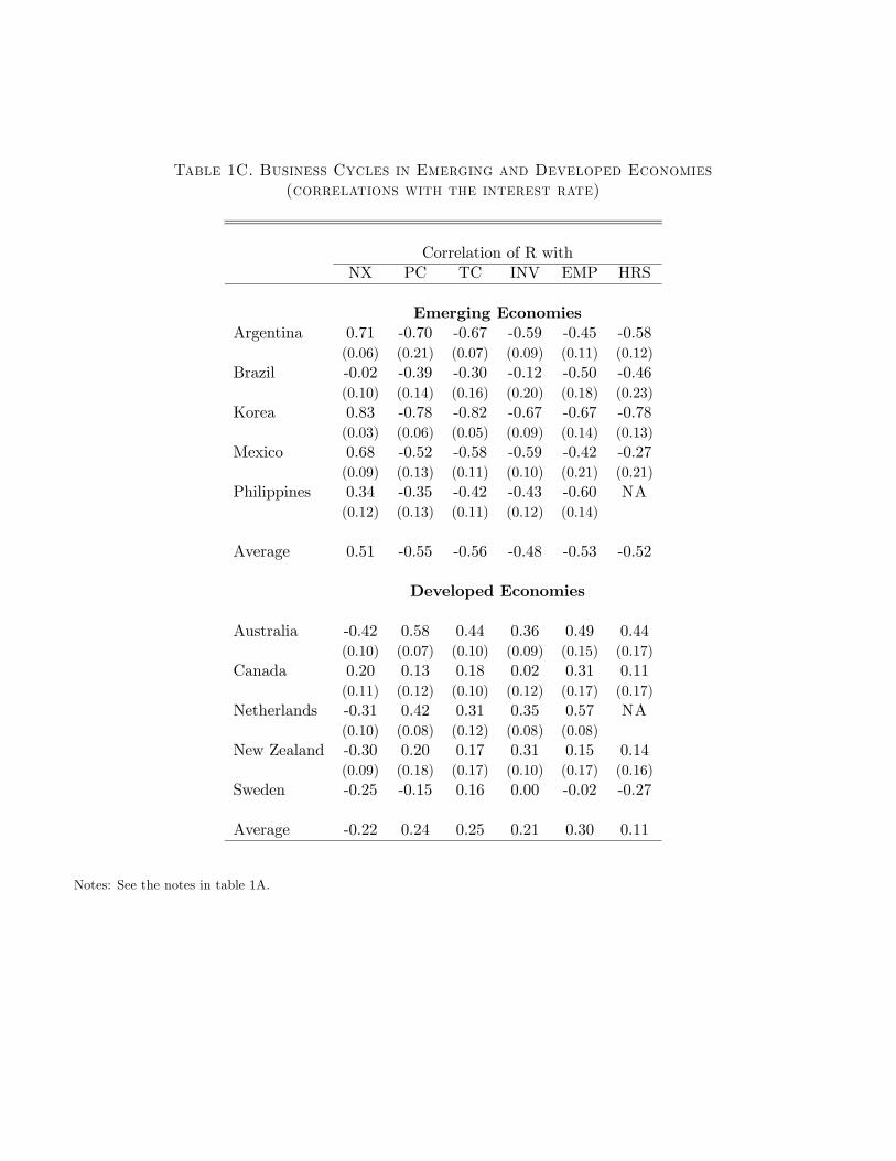
Table 1C. Business Cycles in Emerging and Developed Economies(correlations with the interest rate)

Correlation of R withNX PC TC INV EMP HRS

Emerging EconomiesArgentina 0.71 -0.70 -0.67 -0.59 -0.45 -0.58

(0.06) (0.21) (0.07) (0.09) (0.11) (0.12)Brazil -0.02 -0.39 -0.30 -0.12 -0.50 -0.46

(0.10) (0.14) (0.16) (0.20) (0.18) (0.23)Korea 0.83 -0.78 -0.82 -0.67 -0.67 -0.78

(0.03) (0.06) (0.05) (0.09) (0.14) (0.13)Mexico 0.68 -0.52 -0.58 -0.59 -0.42 -0.27

(0.09) (0.13) (0.11) (0.10) (0.21) (0.21)Philippines 0.34 -0.35 -0.42 -0.43 -0.60 NA

(0.12) (0.13) (0.11) (0.12) (0.14)

Average 0.51 -0.55 -0.56 -0.48 -0.53 -0.52

Developed Economies

Australia -0.42 0.58 0.44 0.36 0.49 0.44(0.10) (0.07) (0.10) (0.09) (0.15) (0.17)

Canada 0.20 0.13 0.18 0.02 0.31 0.11(0.11) (0.12) (0.10) (0.12) (0.17) (0.17)

Netherlands -0.31 0.42 0.31 0.35 0.57 NA(0.10) (0.08) (0.12) (0.08) (0.08)

New Zealand -0.30 0.20 0.17 0.31 0.15 0.14(0.09) (0.18) (0.17) (0.10) (0.17) (0.16)

Sweden -0.25 -0.15 0.16 0.00 -0.02 -0.27

Average -0.22 0.24 0.25 0.21 0.30 0.11

Notes: See the notes in table 1A.

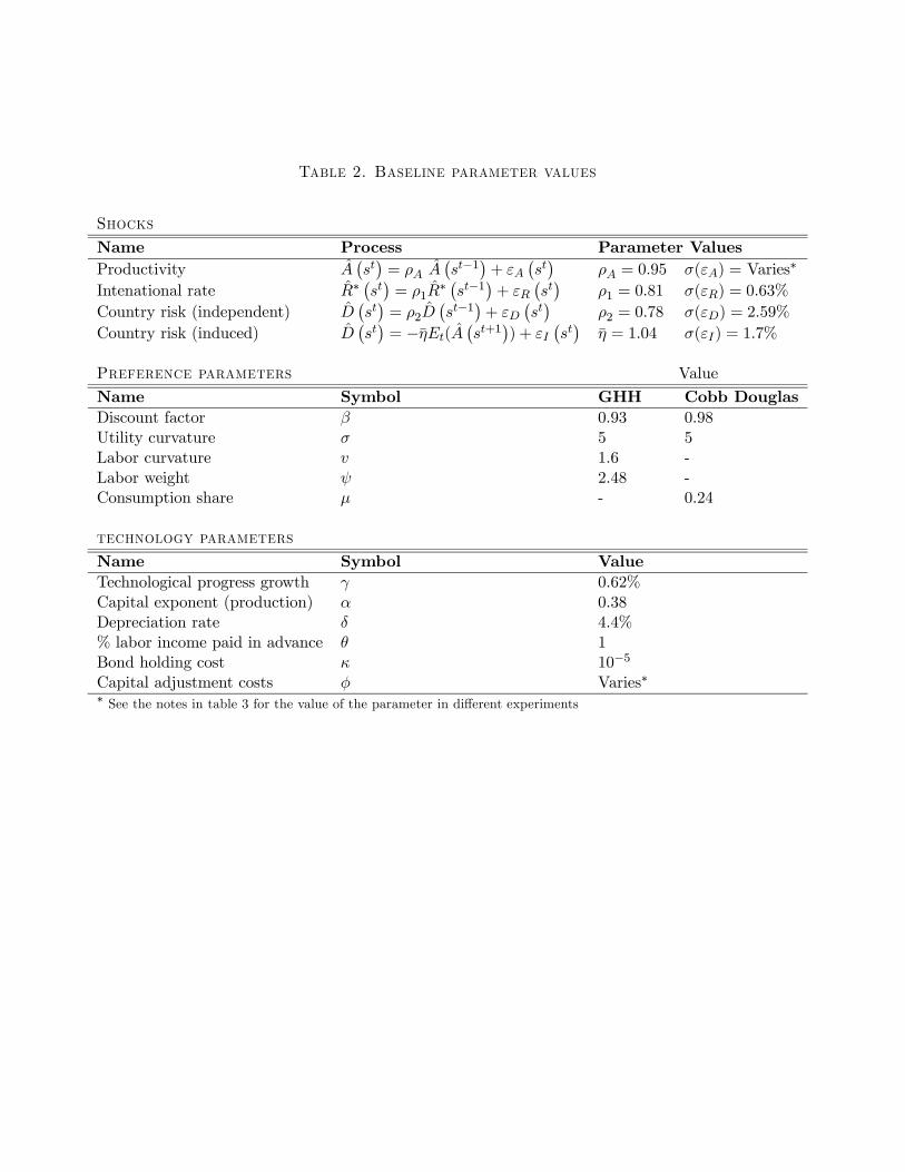
Table 2. Baseline parameter values

Shocks

Name Process Parameter ValuesProductivity A

¡st¢= ρA A

¡st−1

¢+ εA

¡st¢

ρA = 0.95 σ(εA) = Varies∗

Intenational rate R∗¡st¢= ρ1R

∗ ¡st−1¢+ εR¡st¢

ρ1 = 0.81 σ(εR) = 0.63%

Country risk (independent) D¡st¢= ρ2D

¡st−1

¢+ εD

¡st¢

ρ2 = 0.78 σ(εD) = 2.59%

Country risk (induced) D¡st¢= −ηEt(A

¡st+1

¢) + εI

¡st¢

η = 1.04 σ(εI) = 1.7%

Preference parameters Value

Name Symbol GHH Cobb DouglasDiscount factor β 0.93 0.98Utility curvature σ 5 5Labor curvature v 1.6 -Labor weight ψ 2.48 -Consumption share µ - 0.24

technology parameters

Name Symbol ValueTechnological progress growth γ 0.62%Capital exponent (production) α 0.38Depreciation rate δ 4.4%% labor income paid in advance θ 1Bond holding cost κ 10−5

Capital adjustment costs φ Varies∗∗ See the notes in table 3 for the value of the parameter in different experiments

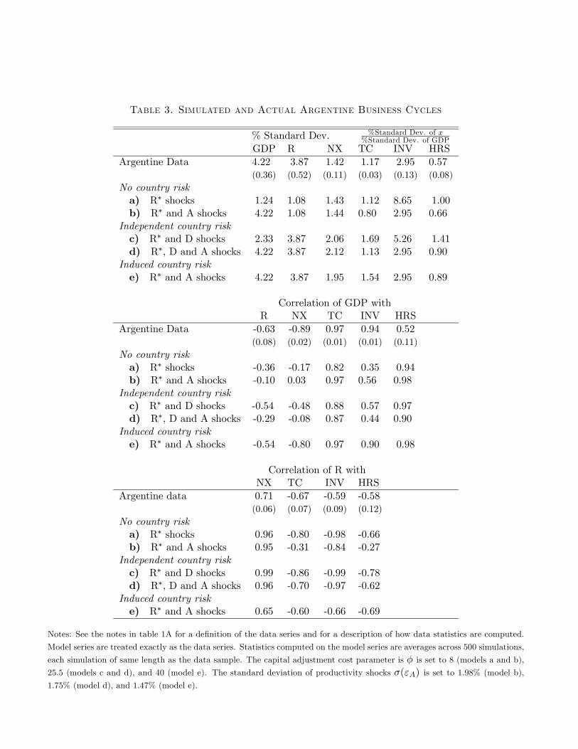
Table 3. Simulated and Actual Argentine Business Cycles

% Standard Dev. %Standard Dev. of x%Standard Dev. of GDP

GDP R NX TC INV HRSArgentine Data 4.22 3.87 1.42 1.17 2.95 0.57

(0.36) (0.52) (0.11) (0.03) (0.13) (0.08)No country riska) R∗ shocks 1.24 1.08 1.43 1.12 8.65 1.00b) R∗ and A shocks 4.22 1.08 1.44 0.80 2.95 0.66

Independent country riskc) R∗ and D shocks 2.33 3.87 2.06 1.69 5.26 1.41d) R∗, D and A shocks 4.22 3.87 2.12 1.13 2.95 0.90

Induced country riske) R∗ and A shocks 4.22 3.87 1.95 1.54 2.95 0.89

Correlation of GDP withR NX TC INV HRS

Argentine Data -0.63 -0.89 0.97 0.94 0.52(0.08) (0.02) (0.01) (0.01) (0.11)

No country riska) R∗ shocks -0.36 -0.17 0.82 0.35 0.94b) R∗ and A shocks -0.10 0.03 0.97 0.56 0.98

Independent country riskc) R∗ and D shocks -0.54 -0.48 0.88 0.57 0.97d) R∗, D and A shocks -0.29 -0.08 0.87 0.44 0.90

Induced country riske) R∗ and A shocks -0.54 -0.80 0.97 0.90 0.98

Correlation of R withNX TC INV HRS

Argentine data 0.71 -0.67 -0.59 -0.58(0.06) (0.07) (0.09) (0.12)

No country riska) R∗ shocks 0.96 -0.80 -0.98 -0.66b) R∗ and A shocks 0.95 -0.31 -0.84 -0.27

Independent country riskc) R∗ and D shocks 0.99 -0.86 -0.99 -0.78d) R∗, D and A shocks 0.96 -0.70 -0.97 -0.62

Induced country riske) R∗ and A shocks 0.65 -0.60 -0.66 -0.69

Notes: See the notes in table 1A for a definition of the data series and for a description of how data statistics are computed.

Model series are treated exactly as the data series. Statistics computed on the model series are averages across 500 simulations,

each simulation of same length as the data sample. The capital adjustment cost parameter is φ is set to 8 (models a and b),

25.5 (models c and d), and 40 (model e). The standard deviation of productivity shocks σ(εA) is set to 1.98% (model b),

1.75% (model d), and 1.47% (model e).

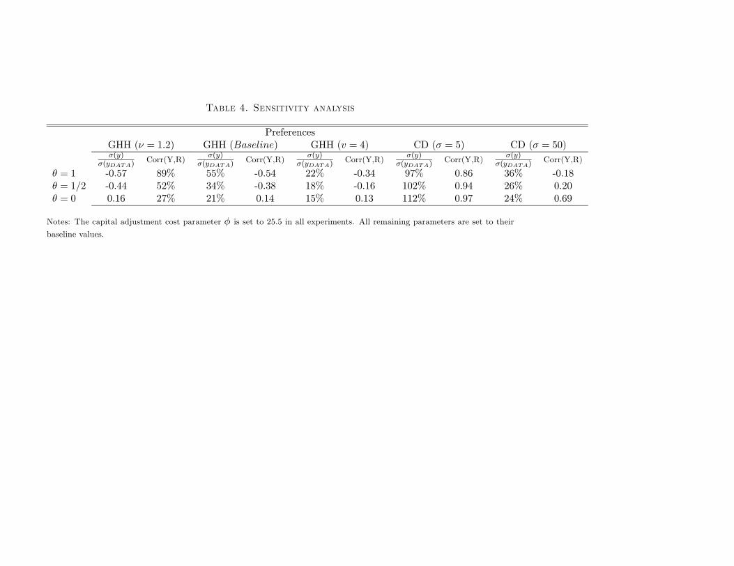
Table 4. Sensitivity analysis

PreferencesGHH (ν = 1.2) GHH (Baseline) GHH (v = 4) CD (σ = 5) CD (σ = 50)σ(y)

σ(yDATA)Corr(Y,R)

σ(y)σ(yDATA)

Corr(Y,R)σ(y)

σ(yDATA)Corr(Y,R)

σ(y)σ(yDATA)

Corr(Y,R)σ(y)

σ(yDATA)Corr(Y,R)

θ = 1 -0.57 89% 55% -0.54 22% -0.34 97% 0.86 36% -0.18θ = 1/2 -0.44 52% 34% -0.38 18% -0.16 102% 0.94 26% 0.20θ = 0 0.16 27% 21% 0.14 15% 0.13 112% 0.97 24% 0.69

Notes: The capital adjustment cost parameter φ is set to 25.5 in all experiments. All remaining parameters are set to their

baseline values.

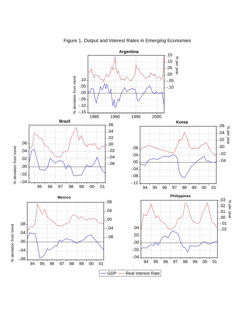
-.15-.10-.05.00.05.10

-.10-.05.00.05.10.15

1985 1990 1995 2000

Argentina

% d

evia

tion

from

tren

d

% per year

-.04

-.02

.00

.02

.04

.06

-.06-.04-.02.00.02.04.06

95 96 97 98 99 00 01

Brazil

% d

evia

tion

from

tren

d

-.12-.08-.04.00.04.08

-.04-.02.00.02.04.06

94 95 96 97 98 99 00 01

Korea % per year

-.08

-.04

.00

.04

.08

-.08

-.04

.00

.04

.08

94 95 96 97 98 99 00 01

Mexico

% d

evia

tion

from

tren

d

-.04

-.02

.00

.02

.04 -.02-.01.00.01.02.03

94 95 96 97 98 99 00 01

GDP Real Interest Rate

Philippines

% per year

Figure 1. Output and Interest Rates in Emerging Economies

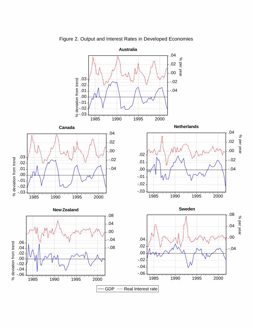
-.03-.02-.01.00.01.02.03

-.04

-.02

.00

.02

.04

1985 1990 1995 2000

Australia

% d

evia

tion

from

tren

d%

per year

-.03-.02-.01.00.01.02.03

-.04

-.02

.00

.02

.04

1985 1990 1995 2000

Canada

% d

evia

tion

from

tren

d

-.03

-.02

-.01

.00

.01

.02

-.04

-.02

.00

.02

.04

1985 1990 1995 2000

Netherlands

% per year

-.06-.04-.02.00.02.04.06

-.08

-.04

.00

.04

.08

1985 1990 1995 2000

New Zealand

% d

evia

tion

from

tren

d

-.06-.04-.02.00.02.04

-.04

.00

.04

.08

1985 1990 1995 2000

GDP Real Interest rate

Sweden

% per year

Figure 2. Output and Interest Rates in Developed Economies

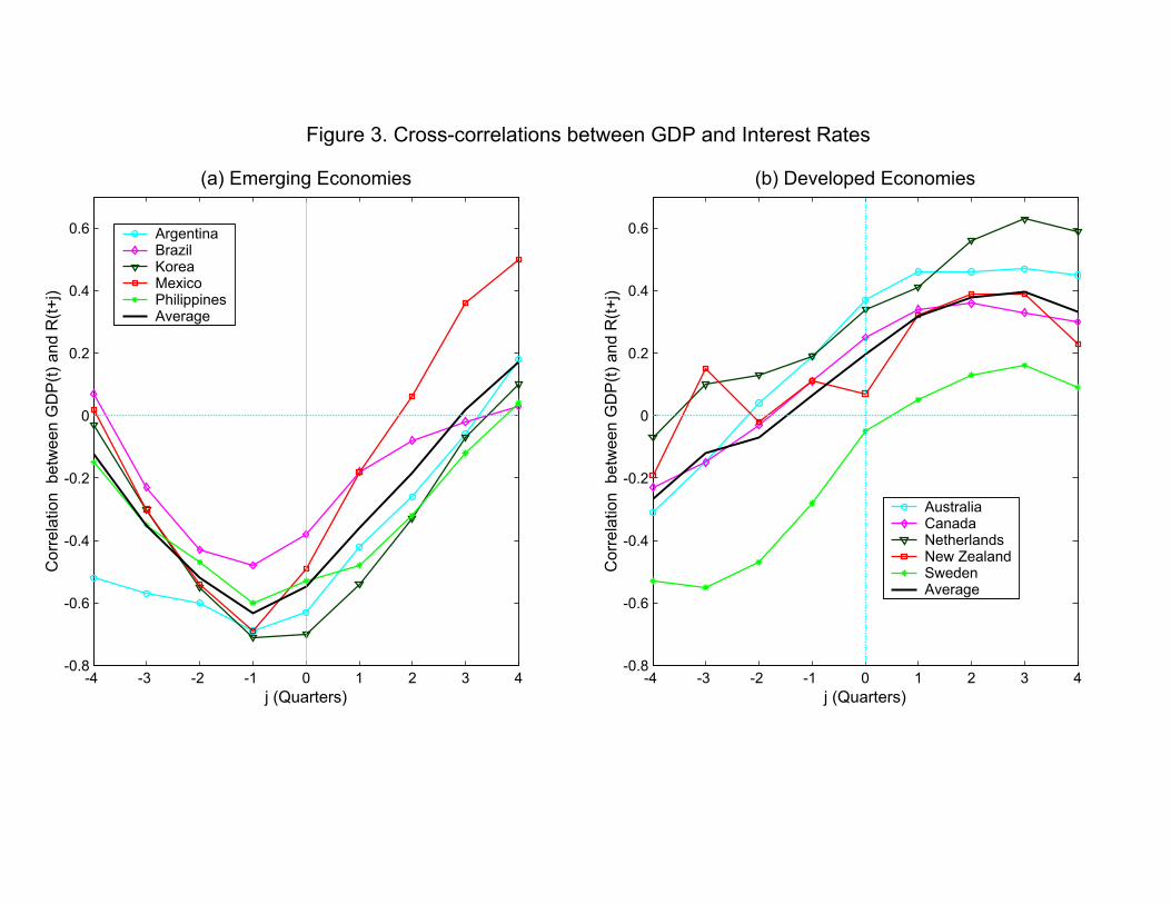
-4 -3 -2 -1 0 1 2 3 4-0.8

-0.6

-0.4

-0.2

0

0.2

0.4

0.6

Figure 3. Cross-correlations between GDP and Interest Rates

(a) Emerging Economies

Cor

rela

tion

bet

wee

n G

DP

(t) a

nd R

(t+j)

j (Quarters)

ArgentinaBrazilKoreaMexicoPhilippinesAverage

-4 -3 -2 -1 0 1 2 3 4-0.8

-0.6

-0.4

-0.2

0

0.2

0.4

0.6

(b) Developed Economies

Cor

rela

tion

bet

wee

n G

DP

(t) a

nd R

(t+j)

j (Quarters)

AustraliaCanadaNetherlandsNew ZealandSwedenAverage

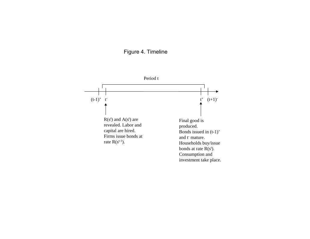
Period t

(t-1)+ t- t+

R(st) and A(st) are revealed. Labor and capital are hired.Firms issue bonds at rate R(st-1).

Final good is produced. Bonds issued in (t-1)+

and t- mature. Households buy/issue bonds at rate R(st).Consumption and investment take place.

(t+1)-

Figure 4. Timeline

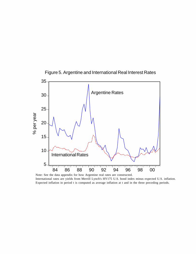
5

10

15

20

25

30

35

84 86 88 90 92 94 96 98 00

Figure 5. Argentine and International Real Interest Rates

Argentine Rates

International Rates

% p

er y

ear

Note: See the data appendix for how Argentine real rates are constructed.International rates are yields from Merrill Lynch's HY175 U.S. bond index minus expected U.S. inflation.Expected inflation in period t is computed as average inflation at t and in the three preceding periods.

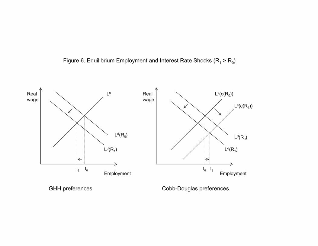
Ld(R0)

Ld(R1)

Employment

Real wage

Ld(R0)

Ld(R1)

Employment

Real wage

Ls(c(R1))

Ls(c(R0))

l0 l1l1 l0

GHH preferences Cobb-Douglas preferences

Figure 6. Equilibrium Employment and Interest Rate Shocks (R1 > R0)

Ls

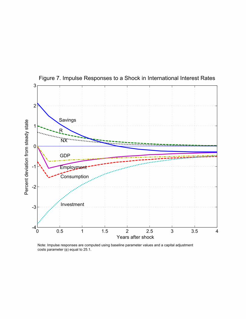
0 0.5 1 1.5 2 2.5 3 3.5 4-4

-3

-2

-1

0

1

2

3Figure 7. Impulse Responses to a Shock in International Interest Rates

Years after shock

Per

cent

dev

iatio

n fro

m s

tead

y st

ate

R

Consumption

Investment

Employment

GDP

NX

Savings

Note: Impulse responses are computed using baseline parameter values and a capital adjustment costs parameter (φ) equal to 25.1.

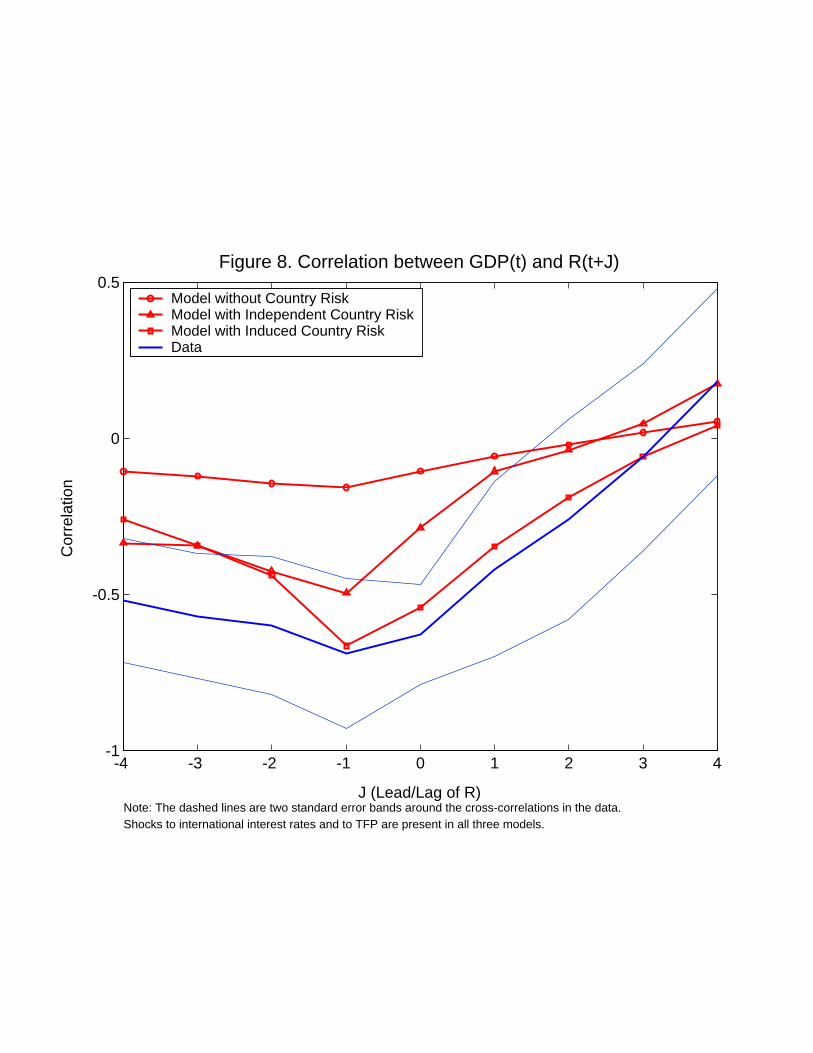
-4 -3 -2 -1 0 1 2 3 4-1

-0.5

0

0.5Figure 8. Correlation between GDP(t) and R(t+J)

J (Lead/Lag of R)

Cor

rela

tion

Note: The dashed lines are two standard error bands around the cross-correlations in the data.Shocks to international interest rates and to TFP are present in all three models.

Model without Country RiskModel with Independent Country RiskModel with Induced Country RiskData

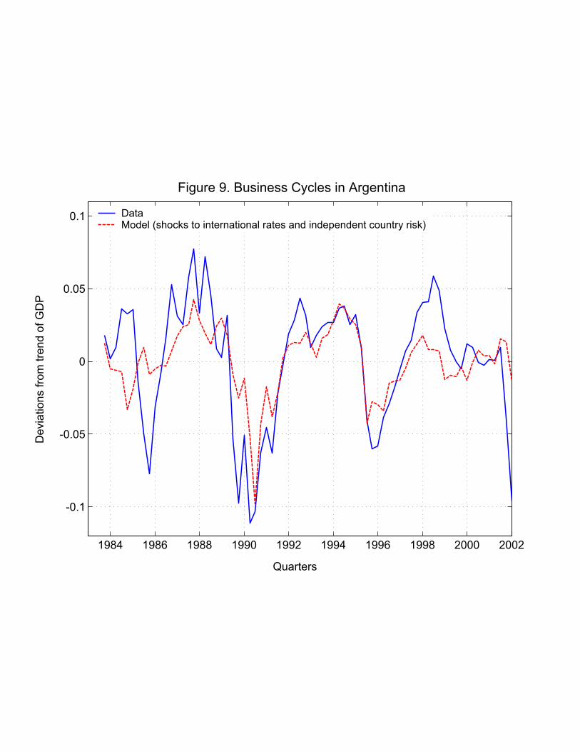
1984 1986 1988 1990 1992 1994 1996 1998 2000 2002

-0.1

-0.05

0

0.05

0.1

Output Cycles in Argentina

Quarters

Dev

iatio

ns fr

om tr

end

of G

DP

DataModel (shocks to international rates and independent country risk)

Figure 9. Business Cycles in Argentina