Business Cycles in Emerging Markets: The Role of

Durable Goods and Financial Frictions

Fernando Alvarez-Parra, Luis Brandao-Marques, and Manuel Toledo∗

April 27, 2011

Abstract

This paper examines how durable goods and financial frictions shape the business cycle

of a small open economy subject to shocks to trend and transitory shocks. The simulation

of the model implies that shocks to trend play a less important role than previously docu-

mented. Financial frictions improve the ability of the model to match some key business

cycle properties of emerging economies. A countercyclical borrowing premium interacts

with the nature of durable goods delivering highly volatile consumption and very counter-

cyclical net exports.

1 Introduction

The business cycle in emerging market economies is characterized by a strongly countercycli-

cal current account and by sovereign interest rates which are also highly countercyclical, very∗We have benefited from comments by participants of the 2008 WEGMANS Conference in Rochester, NY,

the 2009 SED Meetings, in Istanbul, and the IV REDg-DGEM Workshop, in Barcelona. We thank Pravin Krishnaand Mico Loretan for helpful discussions. Alvarez-Parra is affiliated with the Corporacion Andina de Fomento.Brandao-Marques is affiliated with the International Monetary Fund. Toledo is affiliated with the Department ofEconomics, Universidad Carlos III de Madrid, and is grateful to the Spanish Ministry of Science and Innovationfor financial support through grant Juan de la Cierva. The views expressed herein are those of the authors andshould not attributed to CAF, the International Monetary Fund, its Executive Board, or its management.

1

volatile, and significantly higher than the World interest rate. In addition, total consumption

expenditure volatility exceeds income volatility. Aguiar and Gopinath (2007) report that con-

sumption is 40 percent more volatile than income for emerging economies, while slightly less

volatility than income for developed economies. This fact is known as the excess volatility of

consumption puzzle.

The ultimate goal of this paper is to explore possible explanations for business cycle reg-

ularities observed in emerging market economies when considering the existence of both con-

sumer durable and nondurable goods. For this effect, we build a model which combines shocks

to trend and shocks to cycle (Aguiar and Gopinath, 2007) with financial frictions and durable

goods. The disaggregation of consumption into durable and nondurable goods imposes some

discipline to our calibration exercises and creates a channel through which shocks can deliver

more countercyclical net exports and more volatile expenditure in durable goods. We calibrate

the model to match key business cycle facts for Mexico.

One leading explanation for these regularities relies on shocks to trend growth. Aguiar and

Gopinath (2007) find that a standard equilibrium model is consistent with the cyclical proper-

ties of emerging economies once the income process incorporates shocks to trend in addition

to transitory fluctuations around the trend. The intuition comes from the permanent income

hypothesis: a change in the trend of income implies a stronger response of consumption than

a transitory fluctuation around the trend. They conclude that the business cycle in emerging

economies is principally driven by shocks to trend growth. However, we show this result does

not hold once we add durable goods to the consumption bundle.

Limited access to international borrowing and other shocks which directly or indirectly

affect external interest rates have also been used as an explanations for the puzzle. This is a

natural driving force because empirical findings indicate a strong relation between sovereign

interest rates and output. In early real business cycle models for small open economies, interest

rates disturbances play a minor role in driving the business cycle (Mendoza, 1991). When one

2

adds endogenous borrowing limits to a model of a small open economy, however, consump-

tion volatility increases substantially as savings cannot be used to smooth consumption when

the borrowing limit binds (De Resende, 2006). Alternatively, the excessive volatility of con-

sumption can be explained with a financial friction in the form of a working capital borrowing

requirement (Neumeyer and Perri, 2005). In this case, a countercyclical borrowing premium

amplifies the variability of consumption because it makes the demand for labor more sensitive

to the interest rate. Furthermore, shocks to the volatility of the borrowing premium also play

a significant role in explaining the volatility of consumption in emerging market economies

(Fernandez-Villaverde, Guerron-Quintana, Rubio-Ramırez, and Uribe, 2009).1 None of these

papers, however, consider durable goods.

Other papers in the literature study the importance of durables in shaping business cycles

in small open economies. For instance, De Gregorio, Guidotti, and Vegh (1998) study inflation

stabilization programs in emerging market economies and the consumption of durable goods.

There, a boom-recession cycle in consumption is generated through the wealth effect associated

with disinflation (in a cash-in-advance economy) and the existence of non-convex adjustment

costs for the purchase of durables. For the large open economy case, Engel and Wang (2011)

present a two-country model with durables and nondurables and use it to study the volatility

and cyclicality of exports and imports in the United States. Just as we do, they also exploit the

fact that, while durables are mostly tradable, nondurables are not. Neither De Gregorio et al.

nor Engel and Wang, however, explore the joint role of financial frictions and durable goods in

shaping emerging markets business cycles.2

Besides Aguiar and Gopinath (2007), our paper relates most to Neumeyer and Perri (2005)

and to Garcıa-Cicco, Pancrazi, and Uribe (2010). Unlike the latter two, however, we stress the1There are other explanations for the emerging market consumption volatility puzzle which are not explored

here. For instance, Boz, Daude, and Durdu (2008) extend Aguiar and Gopinath’s (2007) model to include imper-fect information and Restrepo-Echevarria (2008) explores the role of the informal economy.

2It is true that the wealth effect created by falling inflation present in De Gregorio et al.’s work can be un-derstood as a type of financial friction. Their model, however, only applies to exchange rate-based stabilizationprograms and not to emerging markets’ business cycles in general.

3

importance of financial frictions in the presence of durable goods. The interaction between

financial frictions and durable goods is important in explaining the dynamics of emerging

markets’ business cycles. This is so because the flow of services coming from the stock of

durables yields utility over time; as a consequence, at least part of the purchase of durables that

take place today can be seen as postponed consumption (i.e., saving).3 Therefore, the purchase

of durable consumption goods should response strongly to the interest rate. If the latter is

countercyclical, an economic expansion caused by a temporary income shock will encourage

consumers to borrow from abroad to take advantage of better credit conditions and thus finance

the acquisition of durables. This generates highly volatile purchases of durables and a strongly

countercyclical trade balance.

The present paper enhances our understanding of business cycles in emerging markets. In

terms of empirical regularities we find that, after decomposing consumption into durables and

nondurables, the excess volatility of consumption puzzle is explained away in the sense that

nondurable consumption is not more volatile than income either in emerging or in developed

economies. In particular, we find that the ratio of the standard deviation of nondurable con-

sumption relative to that of income is 0.9, for a sample of emerging economies, and 0.72, for

a sample of developed economies. Furthermore, our quantitative exercises show that, with

durable and nondurable goods, the role played by shocks to trend as a driving force for the cy-

cle in emerging economies seems smaller than what is found in Aguiar and Gopinath (2007).

We show that a financial friction in the form of a countercyclical borrowing premium (in the

sense of the induced country risk hypothesis suggested by Neumeyer and Perri, 2005) vastly

improves the model’s ability to match the key business cycle moments in Mexico while, at the

same, greatly reduces the importance of shocks to trend. So, at this stage, we can claim that

in order to account for the main characteristics of business cycles in developing economies we

need to consider explicit financial frictions and not rely only on the properties of the technology

3A similar hypothesis has been tested, for instance, by Rosenzweig and Wolpin (1993), according to whom,farmers in India use a durable capital good (bullocks) as the primary vehicle for saving and dissaving.

4

shocks affecting the economy.

The rest of the paper is organized as follows. In the next section, we present some stylized

facts about business cycles in open economies. In Section 3, we set up a dynamic equilib-

rium model where preferences are defined over nondurables, durables, and leisure, and where

technological shocks include an aggregate shock to trend and two sector-specific shocks to

the cycle. Section 4 describes the calibration procedure and Section 5 presents the results.

Section 6 concludes.

2 Data and Stylized Facts

2.1 Data

Our sample is restricted to the countries for which we are able to find data on durable goods’

spending. We split the sample in three groups: small developed economies (Canada, Den-

mark, Finland, Netherlands, New Zealand, and Spain), large developed economies (France,

Italy, Japan, United Kingdom, and United States), and emerging market economies (Chile,

Colombia, Czech Republic, Israel, Mexico, Taiwan Province of China, and Turkey). For each

country we collect data (in real terms) on gross domestic product, total private consumption

expenditure, consumption of nondurable goods, expenditure in durable goods, investment, and

the trade balance. All data is quarterly, except for Colombia for which it is annual. Sample

sizes vary and are detailed in Tables 1 and 2.

Our data come from a variety of sources. For the developed economies and the Czech Re-

public, all data is from the OECD’s Quarterly National Accounts, except for the U.S., for which

it is from the Bureau of Economic Analysis. For Chile, data is from Central Bank of Chile.

Data for Colombia comes from DANE - Departamento Administrativo Nacional de Estadıstica.

Data for Israel is from the Bank of Israel and the Central Bureau of Statistics. Mexican data

comes from INEGI - Instituto Nacional de Estadıstica y Geografıa. For Taiwan Province of

5

China, we retrieve the data from National Statistics, Republic of China (Taiwan). Finally, for

Turkey we use data from the Turkish Statistical Institute. All variables are seasonally adjusted

when needed, converted to logs and detrended using the Hoddrick-Prescott filter.

2.2 Facts

When it comes to emerging market economies and small open developed economies, the fol-

lowing stylized facts about the business cycle are often cited in the literature (see Neumeyer

and Perri, 2005, Uribe and Yue, 2006, Aguiar and Gopinath, 2007, and Garcıa-Cicco et al.,

2010):

1. Real interest rates are countercyclical and leading in emerging markets and acyclical and

lagging in developed economies;

2. Emerging market economies have higher volatilities of output and consumption when

compared to developed economies;

3. Consumption expenditure is more volatile than output in emerging markets while it is

not (quite) as volatile as output in developed economies;

4. Net exports are more volatile and more countercyclical in emerging markets when com-

pared to developed economies.

To these facts we add the following concerning spending in nondurables and durable goods,

based on our sample:

• Consumption of nondurables is not more volatile than output in either small open economies

or emerging markets. We find that the ratio of standard deviation of consumption-to in-

come is 0.9, for a sample of emerging economies, and 0.72, for a sample of developed

economies (see Table 3);

• Spending in durable goods is much more volatile than output in both sets of economies;

6

• Overall, consumption spending in both durables and nondurables is relatively more volatile

in emerging markets than in developed economies.

Looking at the data in Table 1 in more detail, it becomes apparent that the relative volatil-

ities of total consumption spending (i.e., the ratio of the standard deviation of consumption to

the standard deviation of GDP) and of nondurable consumption show considerable variation

within each group. In the case of the emerging market economies, we have Chile, Israel, and

Turkey at the high end and Taiwan Province of China, Colombia, and the Czech Republic at

the low end. While the low value (1.02 for total consumption and 0.81 for nondurable con-

sumption) of Colombia can be attributed to the annual frequency at which the data is sampled,

the values for Taiwan Province of China (0.80 and 0.92, respectively) and the Czech Republic

(0.98 and 0.88, respectively) deserve further exploration.

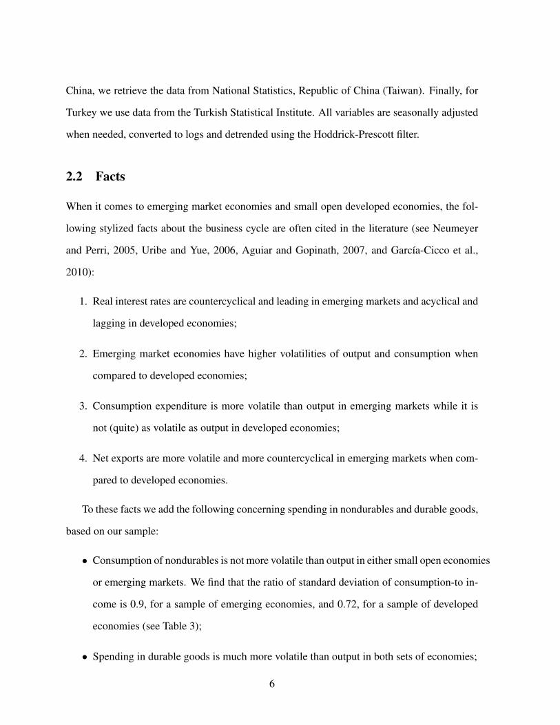
For the Czech Republic one can argue its integration in the European Union and its overall

greater integration into international capital markets made it less sensitive to external shocks

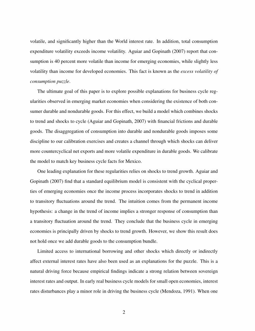
and borrowing constraints. As for Taiwan Province of China, a possible explanation is that its

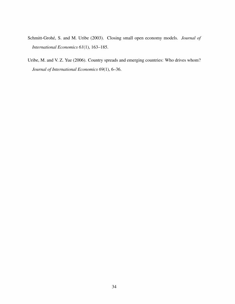
consumers seldom face binding borrowing constraints because of a high saving rate. In Figure

1 we plot the relative volatility of consumption against the average saving rate for the 1960-

1995 period for all countries in our sample.4 Although we do not want to imply any sort of

causation, at this stage, there clearly is a negative relationship. This is an issue we explore more

below, when we deal with the calibration and simulation of a model of a small open economy

with nondurables and durables, with and without financial frictions.

Table 2 shows the same variability within emerging market economies, now in terms of

the correlation of the trade balance with output. While developed economies show uniformly

mildly countercyclical trade balances (in line with the averages of -0.17 and -0.25 for OECD

countries reported by Aguiar and Gopinath, 2007 and Engel and Wang, 2011, respectively),

emerging economies display results which go from mildly procyclical (Taiwan Province of

4Data is from the World Bank’s World Saving Database

7

China at 0.25) to strongly countercyclical net exports (Mexico at -0.82). In fact, the average

correlation of the trade balance with GDP is, in our sample, only -0.20. These results, however,

suffer from a small sample bias as they refer to a group of only a few emerging economies,

somewhat biased towards the most developed countries of that population. With a larger sample

for emerging economies at hand (but for which data on nondurables and durables is missing),

Aguiar and Gopinath find the average correlation between net exports and output to be -0.51.

3 The model

The model we use here is a two-sector neoclassical growth model similar to the one in Aguiar

and Gopinath (2007). In our small open economy, however, there are two types of consumption

goods: durables and nondurables. The nondurable good is assumed to be non-tradable while

the durable good is tradable across borders.5 This assumption is supported by the work of

Engel and Wang (2011) who find that for the average OECD country, the share of durables

in imports and exports (excluding raw materials and energy) is 69 percent and 65 percent,

respectively. For Mexico, these shares increase to 74 percent and 78 percent. So, although

durables represent a smaller fraction of total expenditure than nondurables, they account for

most of the trade in goods.

We assume that markets are incomplete since individuals have only access to one financial

asset, a risk-free bond which pays interest in units of the durable good. Output in each sector is

produced with labor and sector-specific capital. Durables can be used either for consumption or

for capital accumulation. Nondurables can be used for consumption or as intermediate inputs

for the production of durables. The economy is subject to two temporary sectoral aggregate

TFP shocks and one aggregate shock to trend. The technology in the nondurable good sector

5The assumption that nondurable goods are not traded across countries is needed to avoid an overdeterminationarising from the small country assumption for the bond market and factor price equalization across sectors. SeeAppendix A.3 for a more detailed argument.

8

takes the following Cobb-Douglas form:

Yn,t = ezn,tKαnn,t(ΓtLn,t)

1−αn ≡ Fn(Kn,t, Ln,t, zn,t,Γt). (1)

For the durable good sector we assume a production function that combines a nondurable in-

termediate input in fixed proportions with capital and labor. This assumption of zero elasticity

of substitution between the intermediate input and the value added component (which depends

on capital and labor) is common in static general equilibrium models and seems to be appro-

priate for a dynamic setting as well.6 The value-added component for durables depends on

capital and labor combined as in a Cobb-Douglas production function. The technology for the

production of durables is

Yd,t = minezd,tKαd

d,t (ΓtLd,t)1−αd︸ ︷︷ ︸

≡Fd(Kd,t,Ld,t,zd,t,Γt)

;Mn,t

Ω

, (2)

where Mn,t is the nondurable intermediate input used in the production of the durable good

and Ω is the number of units of the intermediate input needed to produce one unit of the

durable good (see Kehoe and Kehoe, 1994). The presence of intermediate goods acknowledges

the important inter-sectoral links that characterize modern industrial economies. Moreover,

studies show that explicitly accounting for such relations in a model improves its ability to

reproduce some business cycle regularities; in particular, the comovement in output among

sectors (Hornstein and Praschnik, 1997). In (1) and (2), Γt is the common trend and Ki,t and

Li,t denote capital and labor inputs, αi ∈ (0, 1) represents the capital’s share of output, and zi,t

is the temporary stochastic productivity process in sector i, for i ∈ n, d. As in Aguiar and

Gopinath (2007), Γt = Γt−1egt , where gt is the (stationary) shock to trend. It is assumed that

6Using a dynamic general equilibrium model at quarterly frequency, Kouparitsas (1998) estimates the elasticityof substitution between these two components at 0.1, which is very close to the Leontief case.

9

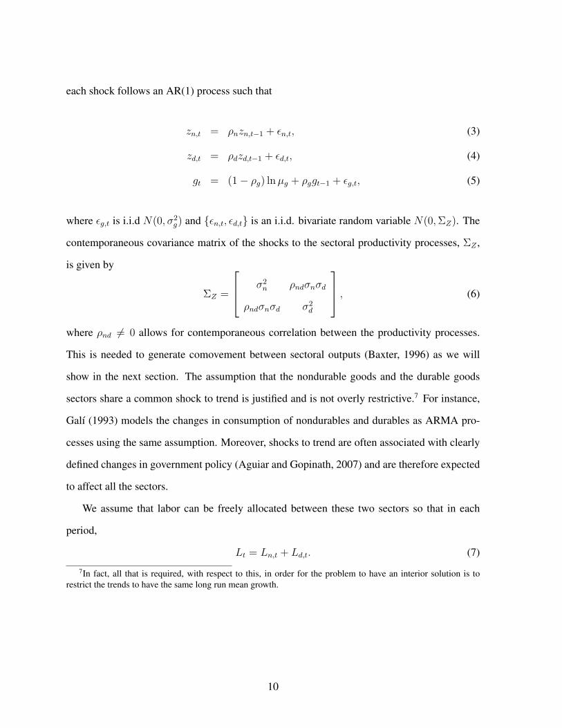
each shock follows an AR(1) process such that

zn,t = ρnzn,t−1 + εn,t, (3)

zd,t = ρdzd,t−1 + εd,t, (4)

gt = (1− ρg) lnµg + ρggt−1 + εg,t, (5)

where εg,t is i.i.d N(0, σ2g) and εn,t, εd,t is an i.i.d. bivariate random variable N(0,ΣZ). The

contemporaneous covariance matrix of the shocks to the sectoral productivity processes, ΣZ ,

is given by

ΣZ =

σ2n ρndσnσd

ρndσnσd σ2d

, (6)

where ρnd 6= 0 allows for contemporaneous correlation between the productivity processes.

This is needed to generate comovement between sectoral outputs (Baxter, 1996) as we will

show in the next section. The assumption that the nondurable goods and the durable goods

sectors share a common shock to trend is justified and is not overly restrictive.7 For instance,

Galı (1993) models the changes in consumption of nondurables and durables as ARMA pro-

cesses using the same assumption. Moreover, shocks to trend are often associated with clearly

defined changes in government policy (Aguiar and Gopinath, 2007) and are therefore expected

to affect all the sectors.

We assume that labor can be freely allocated between these two sectors so that in each

period,

Lt = Ln,t + Ld,t. (7)

7In fact, all that is required, with respect to this, in order for the problem to have an interior solution is torestrict the trends to have the same long run mean growth.

10

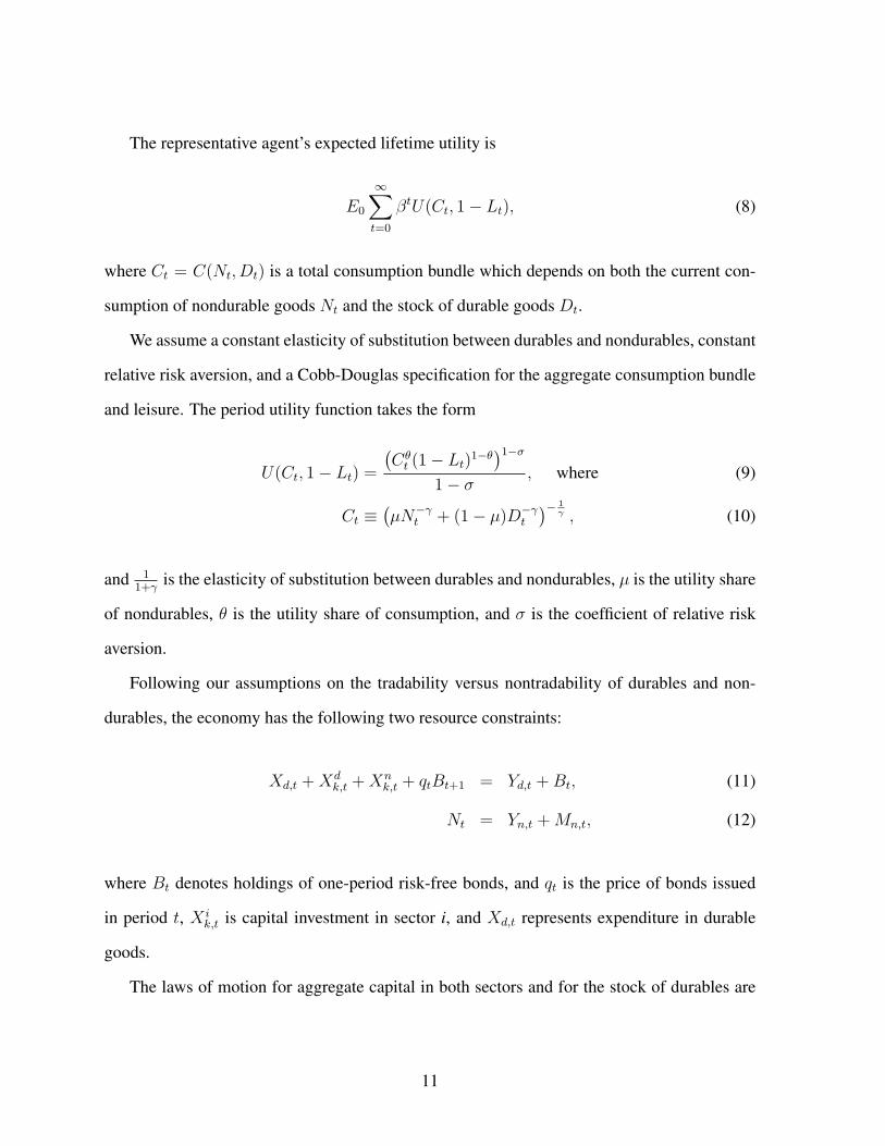
The representative agent’s expected lifetime utility is

E0

∞∑t=0

βtU(Ct, 1− Lt), (8)

where Ct = C(Nt, Dt) is a total consumption bundle which depends on both the current con-

sumption of nondurable goods Nt and the stock of durable goods Dt.

We assume a constant elasticity of substitution between durables and nondurables, constant

relative risk aversion, and a Cobb-Douglas specification for the aggregate consumption bundle

and leisure. The period utility function takes the form

U(Ct, 1− Lt) =

(Cθt (1− Lt)1−θ)1−σ

1− σ, where (9)

Ct ≡(µN−γt + (1− µ)D−γt

)− 1γ , (10)

and 11+γ

is the elasticity of substitution between durables and nondurables, µ is the utility share

of nondurables, θ is the utility share of consumption, and σ is the coefficient of relative risk

aversion.

Following our assumptions on the tradability versus nontradability of durables and non-

durables, the economy has the following two resource constraints:

Xd,t +Xdk,t +Xn

k,t + qtBt+1 = Yd,t +Bt, (11)

Nt = Yn,t +Mn,t, (12)

where Bt denotes holdings of one-period risk-free bonds, and qt is the price of bonds issued

in period t, X ik,t is capital investment in sector i, and Xd,t represents expenditure in durable

goods.

The laws of motion for aggregate capital in both sectors and for the stock of durables are

11

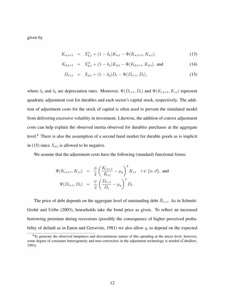
given by

Kn,t+1 = Xnk,t + (1− δk)Kn,t − Φ(Kn,t+1, Kn,t), (13)

Kd,t+1 = Xdk,t + (1− δk)Kd,t − Φ(Kd,t+1, Kd,t), and (14)

Dt+1 = Xd,t + (1− δd)Dt −Ψ(Dt+1, Dt), (15)

where δd and δk are depreciation rates. Moreover, Ψ(Dt+1, Dt) and Φ(Ki,t+1, Ki,t) represent

quadratic adjustment cost for durables and each sector’s capital stock, respectively. The addi-

tion of adjustment costs for the stock of capital is often used to prevent the simulated model

from delivering excessive volatility in investment. Likewise, the addition of convex adjustment

costs can help explain the observed inertia observed for durables purchases at the aggregate

level.8 There is also the assumption of a second hand market for durable goods as is implicit

in (15) since Xd,t is allowed to be negative.

We assume that the adjustment costs have the following (standard) functional forms:

Φ(Ki,t+1, Ki,t) =φ

2

(Ki,t+1

Ki,t

− µg)2

Ki,t i ∈ n, d, and

Ψ(Dt+1, Dt) =ψ

2

(Dt+1

Dt

− µg)2

Dt.

The price of debt depends on the aggregate level of outstanding debt Bt+1. As in Schmitt-

Grohe and Uribe (2003), households take the bond price as given. To reflect an increased

borrowing premium during recessions (possibly the consequence of higher perceived proba-

bility of default as in Eaton and Gersovitz, 1981) we also allow qt to depend on the expected

8To generate the observed lumpiness and discontinuous nature of this spending at the micro level, however,some degree of consumer heterogeneity and non-convexities in the adjustment technology is needed (Caballero,1993).

12

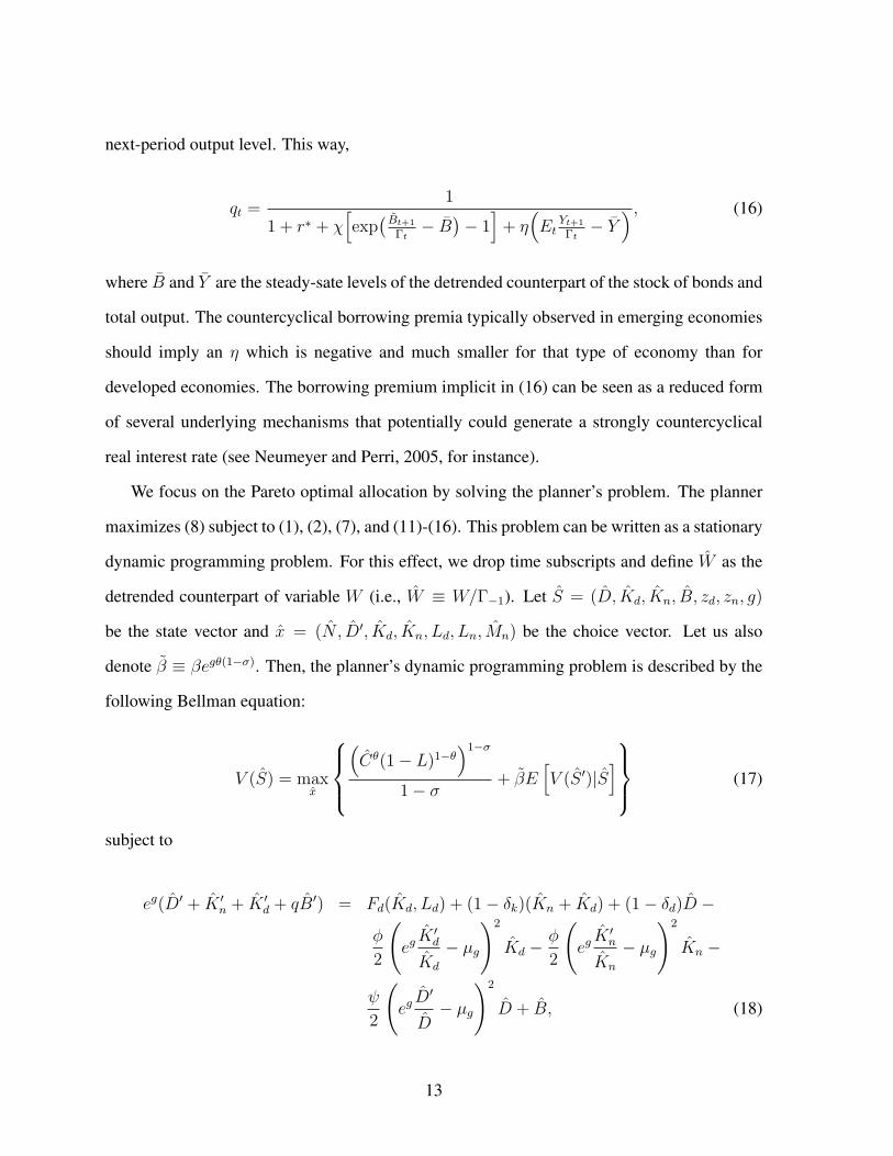
next-period output level. This way,

qt =1

1 + r∗ + χ[exp(Bt+1

Γt− B

)− 1]

+ η(Et

Yt+1

Γt− Y

) , (16)

where B and Y are the steady-sate levels of the detrended counterpart of the stock of bonds and

total output. The countercyclical borrowing premia typically observed in emerging economies

should imply an η which is negative and much smaller for that type of economy than for

developed economies. The borrowing premium implicit in (16) can be seen as a reduced form

of several underlying mechanisms that potentially could generate a strongly countercyclical

real interest rate (see Neumeyer and Perri, 2005, for instance).

We focus on the Pareto optimal allocation by solving the planner’s problem. The planner

maximizes (8) subject to (1), (2), (7), and (11)-(16). This problem can be written as a stationary

dynamic programming problem. For this effect, we drop time subscripts and define W as the

detrended counterpart of variable W (i.e., W ≡ W/Γ−1). Let S = (D, Kd, Kn, B, zd, zn, g)

be the state vector and x = (N , D′, Kd, Kn, Ld, Ln, Mn) be the choice vector. Let us also

denote β ≡ βegθ(1−σ). Then, the planner’s dynamic programming problem is described by the

following Bellman equation:

V (S) = maxx

(Cθ(1− L)1−θ

)1−σ

1− σ+ βE

[V (S ′)|S

] (17)

subject to

eg(D′ + K ′n + K ′d + qB′) = Fd(Kd, Ld) + (1− δk)(Kn + Kd) + (1− δd)D −

φ

2

(egK ′d

Kd

− µg

)2

Kd −φ

2

(egK ′n

Kn

− µg

)2

Kn −

ψ

2

(egD′

D− µg

)2

D + B, (18)

13

N = Fn(Kn, Ln)− Mn, (19)

L = Ln + Ld ≤ 1, (20)

C = (µN−γ + (1− µ)D−γ)−1γ , (21)

nonnegativity constraints Li ≥ 0, K ′i ≥ 0, i ∈ n, d, N ≥ 0, and D′ ≥ 0; and stochastic

processes (3)-(5). Aggregate bond holdings are made consistent with per capital bond holdings

such that B = B. Moreover, the planner takes the bond price q as exogenous as she does not

internalize the effect of B′ on q. This is to be consistent with the fact that households also take

q as given, as mentioned above.

We follow Kehoe and Kehoe (1994) and assume producers minimize costs and earn zero

profits so that we can write

Mn = ΩYd. (22)

Using (22), the first-order optimality conditions coming from this problem are:

UCCNp [1−ΨD′ ] eg = βES UC′ [CD′ + CN ′p

′ (1− δd −Ψ′D′)] , (23)

UCCNp[1− ΦK′n

]eg = βES

UC′CN ′

[Fn,K′ + p′

(1− δk − Φ′K′n

)], (24)

UCCNp[1− ΦK′d

]eg = βES

UC′CN ′

[p′(Fd,K′ + 1− δk − Φ′K′d

)+ ΩFd,K′

], (25)

UCCNpqeg = βES [UC′CN ′p′] , (26)

UCCNFn,L = UL, and (27)

Fn,L = (p− Ω)Fd,L, (28)

where ES = E[·|S] is the conditional expectation operator, UC and UL are the marginal utili-

ties of consumption and leisure, CD and CN are the derivatives of the consumption aggregator

with respect to durables and nondurables, Fi,K and Fi,L are the marginal products of capital

and labor in sector i, and similarly ΨD′ and ΦK′iare the derivatives of the adjustment cost func-

14

tions with respect to D′ and K ′i. Moreover, we define p as the ratio (λd/λn) of the Lagrange

multipliers associated with the resources constraints (18) and (19), which can be interpreted as

the relative price of durables to nondurables.

The first four equations correspond to intertemporal trade-offs between current nondurable

consumption and the accumulation of durable goods, capital and debt. The last two equations

represent static optimality conditions for the consumption-leisure decision and labor allocation

between sectors.

4 Calibration

We calibrate the model to the Mexican economy at quarterly frequency. Our parametrization

follows as much as possible that of Aguiar and Gopinath’ (2007) but accommodates for the

inclusion of durable goods. Specifically, the income share of labor is set to 0.48 for nondurables

and 0.68 for durables, as used in Baxter (1996). From the same source, the annual depreciation

rates for capital and durables are set to 7.1 percent and 15.6 percent, respectively. We set the

intermediate input coefficient Ω to 0.3 which is close to what Kouparitsas (1998) documents

for Mexico (0.28) and within the range (between 0.26 and 0.38, depending on the measure)

observed for the U.S. by Hornstein and Praschnik (1997).

The utility share of nondurables (µ) is set to 0.881 to match the average share of consump-

tion of nondurable goods in total consumption expenditure of 91.8 percent. The Cobb-Douglas

exponent for consumption in the utility function (θ) is set to 0.413 in order to match a steady-

state share of time devoted to work of 1/3. As in Aguiar and Gopinath, we work with a dis-

count factor (β) of 0.98, a coefficient of relative risk aversion (σ) of 2, and a coefficient for

the adjustment costs of the capital stocks (φ) of 4. From the same paper we take the means

and autocorrelation coefficients for the error processes (µg,ρg,ρn, and ρd). Following Gomes,

Kogan, and Yogo (2009), the elasticity of substitution(

11+γ

)is set to 0.86.9

9This value means that the two goods are gross substitutes (the condition being σ > 1 + γ/θ). It is also con-

15

The steady-state level of debt relative to GDP (−B/Y ) is fixed at 0.1,10 and the parameter

that determines the sensitivity of the bond price to the debt level, χ, is set to -0.001. The choice

of a small value for χ (but different from zero) is justified with the need to avoid the well-

known unit root problem of net foreign assets in small open economy models (Schmitt-Grohe

and Uribe, 2003) without changing the short-run dynamics. Parameter values are summarized

in Table 4.

We calibrate the remaining parameters - the variances of the TFP shocks (σ2g , σ2

n, and σ2d),

the correlation between shocks to durables and shocks to nondurables (ρnd), the coefficient for

adjustment cost of durables (ψ), and the financial friction parameter (η), by trying to replicate

certain business cycle moments.11 The moments to match vary across different calibration

exercises as described below. The resulting parameter values are shown in Table 5.

5 Results

In this section we investigate the business cycle properties implied by our model economy. To

that end, we first solve the model using a standard first-order log-linearization procedure, and

then compute relevant theoretical moments.12

Table 5 presents business cycle moments for GDP (total value added), sectoral output

(industrial production), total consumption expenditure, nondurable consumption, spending in

durables, the net exports-output ratio, investment, and the borrowing premium. Moreover, we

show a measure of the quality of fit of the simulation (the sum of the square deviations of all

the simulated moments relative to the sample moments, normalized by the total variation of all

sistent with Ogaki and Reinhart’s (1998) finding that the intratemporal elasticity of substitution between durablesand nondurables is significantly higher than the intertemporal elasticity of substitution.

10This parameter only matters to determine the steady-state level of net exports and is immaterial for results.11None of these parameters affect the deterministic steady state around which the linearization is performed.12For this effect, we use Dynare for Matlab Version 4.1. The solution consists of policy functions for the

control variables (consumption of nondurables, spending in durables, output of nondurables and durables, laborfor durables and nondurables, and the relative price of durables) and laws of motion for the endogenous states(capital stocks, durables stock, and bond holdings) as a function of the states and forcing variables (shocks todurables and nondurables and shock to trend).

16

the sample moments) and three measures of the contribution of the permanent shock to non-

durables (wn), to durables (wd), and to the variance of output.13 Each column (1)-(5) displays

the results for a different calibration exercise as we now explain.

5.1 No Financial Frictions Case

Our first exercise is to solve for the variances of the TFP shocks as well as ψ and ρnd to

match the volatilities of GDP, consumption of nondurables, durables expenditure, and the net

exports-GDP ratio as well as the correlation between the two sectoral outputs.14 Here, we stay

as close as possible to Aguiar and Gopinath’s (2007) model. In particular, we set the borrowing

premium parameter η = 0. We call this scenario the no financial frictions case.15 We obtain

σg = 1.8340, σn = 1.4209, σd = 1.4528, ψ = 0.5336 and ρnd = 0.3631, as shown in column

(1) of Table 5, and are able to exactly match the targeted moments (in bold). The estimates of

the random walk component of the sectoral Solow residuals are substantially smaller than what

Aguiar and Gopinath find for Mexico (0.28 and 0.43 for nondurables and durables, respectively

against 0.96). As a result, the permanent shock accounts for about 32 percent of GDP volatility.

As an initial conclusion based on this first simulation results, we find that our framework

does a good job at capturing the high volatility of consumption of nondurables and spending

in durables. It does reasonably well in mimicking the volatility of total consumption spending

and the overall comovement observed in the data.16 The model also delivers a countercyclical

trade balance although it reproduces only about half of what is found in the data. The model

13The first two measures are the random walk components for the nondurable and durable sectors calculatedas in equation (14) of Aguiar and Gopinath’s (2007) paper and the third comes from a variance decomposition ofGDP.

14We use quarterly data for industrial production in the sectors of consumer durables and nondurables. Thisdata is also from INEGI and covers the same sample period as all other data used for Mexico.

15We are aware that the fact that the bond price is sensitive to the aggregate debt level is in itself a financialfriction. As mentioned before, the size of that friction (χ) is set to such a small value that it does not significantlyaffect the short run dynamics of the simulated economy.

16This applies to total hours worked as well since our solution delivers a correlation of 0.76 with GDP whichcompares to 0.90 in the data (total hours worked in manufacturing for the same sample period). This finding isnoteworthy given the difficulty of matching the cyclicality of hours worked in real business cycle models withoutassuming GHH preferences.

17

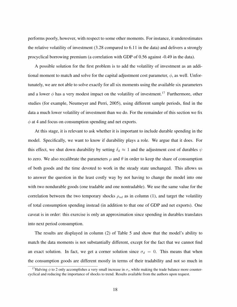
performs poorly, however, with respect to some other moments. For instance, it underestimates

the relative volatility of investment (3.28 compared to 6.11 in the data) and delivers a strongly

procyclical borrowing premium (a correlation with GDP of 0.56 against -0.49 in the data).

A possible solution for the first problem is to add the volatility of investment as an addi-

tional moment to match and solve for the capital adjustment cost parameter, φ, as well. Unfor-

tunately, we are not able to solve exactly for all six moments using the available six parameters

and a lower φ has a very modest impact on the volatility of investment.17 Furthermore, other

studies (for example, Neumeyer and Perri, 2005), using different sample periods, find in the

data a much lower volatility of investment than we do. For the remainder of this section we fix

φ at 4 and focus on consumption spending and net exports.

At this stage, it is relevant to ask whether it is important to include durable spending in the

model. Specifically, we want to know if durability plays a role. We argue that it does. For

this effect, we shut down durability by setting δd ≈ 1 and the adjustment cost of durables ψ

to zero. We also recalibrate the parameters µ and θ in order to keep the share of consumption

of both goods and the time devoted to work in the steady state unchanged. This allows us

to answer the question in the least costly way by not having to change the model into one

with two nondurable goods (one tradable and one nontradable). We use the same value for the

correlation between the two temporary shocks ρnd as in column (1), and target the volatility

of total consumption spending instead (in addition to that one of GDP and net exports). One

caveat is in order: this exercise is only an approximation since spending in durables translates

into next period consumption.

The results are displayed in column (2) of Table 5 and show that the model’s ability to

match the data moments is not substantially different, except for the fact that we cannot find

an exact solution. In fact, we get a corner solution since σd = 0. This means that when

the consumption goods are different mostly in terms of their tradability and not so much in

17Halving φ to 2 only accomplishes a very small increase in σi, while making the trade balance more counter-cyclical and reducing the importance of shocks to trend. Results available from the authors upon request.

18

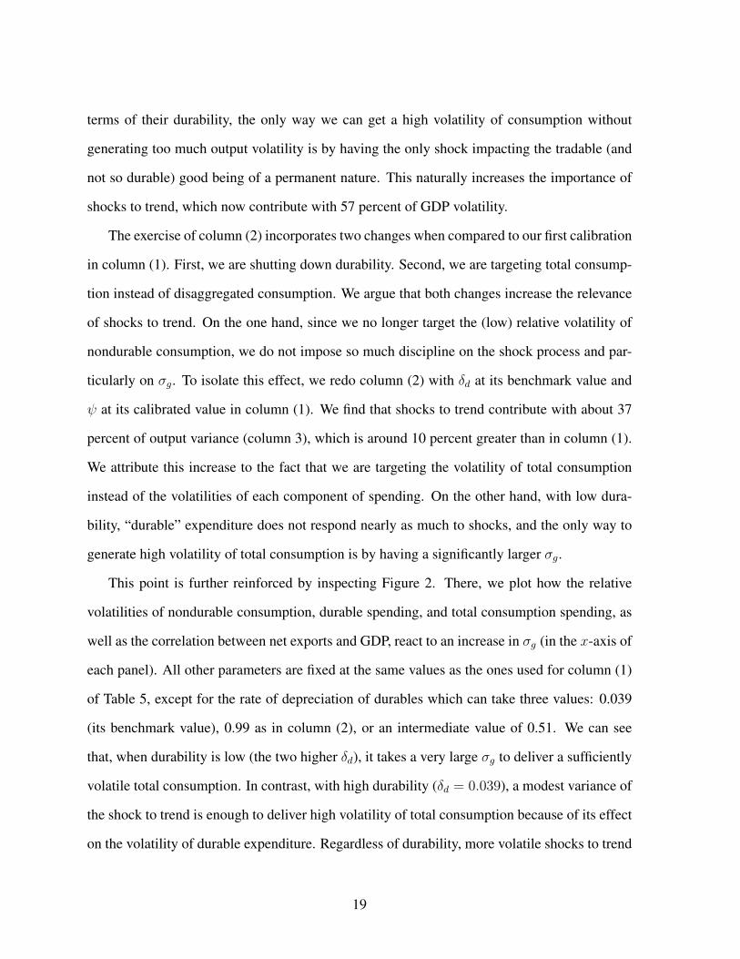
terms of their durability, the only way we can get a high volatility of consumption without

generating too much output volatility is by having the only shock impacting the tradable (and

not so durable) good being of a permanent nature. This naturally increases the importance of

shocks to trend, which now contribute with 57 percent of GDP volatility.

The exercise of column (2) incorporates two changes when compared to our first calibration

in column (1). First, we are shutting down durability. Second, we are targeting total consump-

tion instead of disaggregated consumption. We argue that both changes increase the relevance

of shocks to trend. On the one hand, since we no longer target the (low) relative volatility of

nondurable consumption, we do not impose so much discipline on the shock process and par-

ticularly on σg. To isolate this effect, we redo column (2) with δd at its benchmark value and

ψ at its calibrated value in column (1). We find that shocks to trend contribute with about 37

percent of output variance (column 3), which is around 10 percent greater than in column (1).

We attribute this increase to the fact that we are targeting the volatility of total consumption

instead of the volatilities of each component of spending. On the other hand, with low dura-

bility, “durable” expenditure does not respond nearly as much to shocks, and the only way to

generate high volatility of total consumption is by having a significantly larger σg.

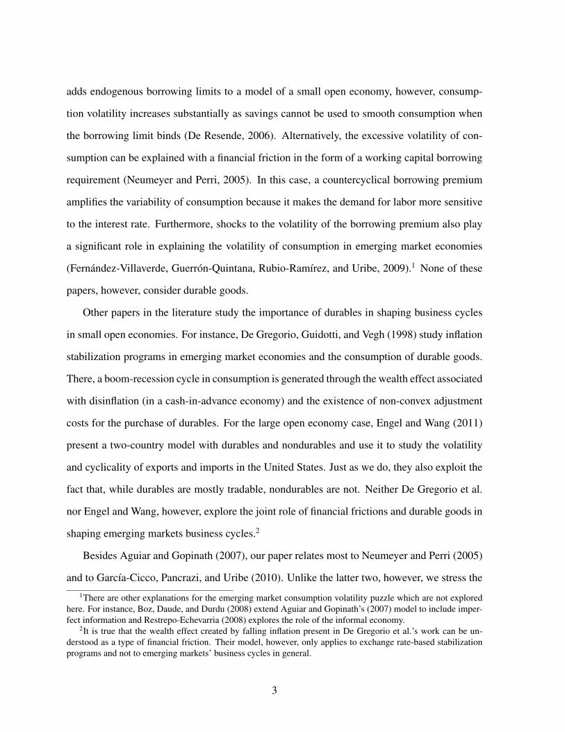
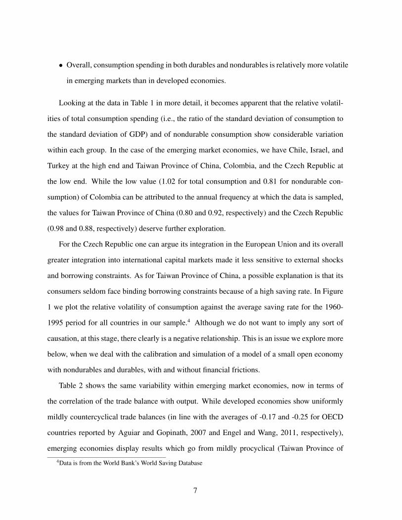
This point is further reinforced by inspecting Figure 2. There, we plot how the relative

volatilities of nondurable consumption, durable spending, and total consumption spending, as

well as the correlation between net exports and GDP, react to an increase in σg (in the x-axis of

each panel). All other parameters are fixed at the same values as the ones used for column (1)

of Table 5, except for the rate of depreciation of durables which can take three values: 0.039

(its benchmark value), 0.99 as in column (2), or an intermediate value of 0.51. We can see

that, when durability is low (the two higher δd), it takes a very large σg to deliver a sufficiently

volatile total consumption. In contrast, with high durability (δd = 0.039), a modest variance of

the shock to trend is enough to deliver high volatility of total consumption because of its effect

on the volatility of durable expenditure. Regardless of durability, more volatile shocks to trend

19

yields a more countercyclical trade balance. However, in order to get a sufficiently negative

correlation of net exports with GDP, the model requires shocks to trend to be so large that

consumption, and particularly durable expenditure, becomes too volatile. This suggests more

is needed in order to match the cyclical behavior of the Mexican trade balance. We explore

next how financial frictions may help in this and other dimensions of the emerging markets’

business cycles.

5.2 Financial Frictions Case

Two dimensions where the model thus far fares poorly are in capturing the volatility of the

borrowing premium (which it grossly underestimates) and in mimicking its countercyclical

behavior (in the first two simulations it comes very procyclical). Here we attempt to discipline

the dynamics of the model in this dimension by introducing financial frictions.

One simple way to do this is to match the volatility of the borrowing premium by choosing

an appropriate value for χ. This is what Garcıa-Cicco et al. (2010) do in a RBC model with

financial frictions but no durables. They do not report, however, the simulated moments for the

borrowing premium and focus on the autocorrelation of net exports.

An alternative way of introducing a financial friction is to have a non-zero income-elasticity

of the borrowing premium, which is defined by the parameter η. A negative value for η implies

a countercyclical borrowing premium and is consistent with what Neumeyer and Perri (2005)

call the induced country risk case. We choose this route instead of calibrating χ because, if we

target the observed correlation of the borrowing premium with output, the latter may introduce

a bias against shocks to trend. The reason for this bias is that a positive permanent shock causes

agents to borrow more and increase their stock of debt which, given χ < 0, causes the borrow-

ing premium to increase as well and, therefore, to be counterfactually procyclical. Therefore,

targeting the cyclical dynamics of the borrowing premium may diminish the importance of

shocks to trend.

20

In column (4), we present the results when we target the volatilities of GDP, nondurables

consumption, expenditure in durables, the net exports-GDP ratio, and the borrowing premium

as well as the correlation between the two sectoral outputs by solving for σg, σn, σd, ψ, ρnd

and η. What we do here is to extend the calibration exercise in column (1) by adding one

parameter (η) and one moment (ρbp,y). First, we should note that we are able to find an exact

solution and that there is a substantial improvement in the quality of fit of the model compared

to column (1). Second, we get an estimate for η of -0.0077, consistent with the induced country

risk hypothesis. Third, even though we were not explicitly targeting this moment, the correla-

tion of net exports-GDP ratio with GDP (at -0.72) gets much closer to its sample counterpart.

Fourth, the importance of the shocks to trend falls, accounting now for about 24 percent of

GDP variance.

The reason why a model with durables and financial frictions is able to deliver more coun-

tercyclical net exports can be found in the interaction between the accumulation of durables

and the countercyclical borrowing premium. The financial friction introduced in our model,

which mimics an empirical fact, implies that interest rates are countercyclical and relatively

more volatile. As a consequence, during booms the economy can take advantage of cheaper

credit by borrowing more to build capital and increase the stock of durables. Since durables

are mostly tradable (another empirical fact), part of the accumulation of durables (and capital)

will resort to imports. As a consequence, net exports fall during economic expansions making

the trade balance countercyclical.

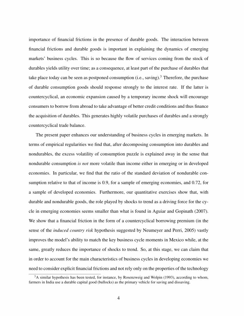
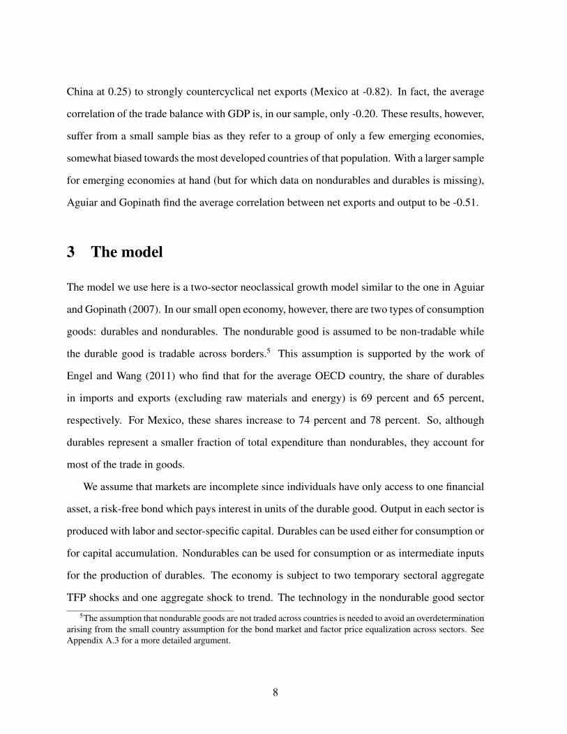
This point is made clear when we compare the impulse-response functions generated by

the model with and without the financial friction, which we present in figures 3 through 5.18 In

Figure 3, we show the response of our model economy to a permanent technology shock. It is

clear that for all variables except the borrowing premium, the financial friction does not play

a significant role when a permanent shock hits the economy. The main intuition why financial

18In these figures, we use the parameters values in column (4) of Table 5 unless otherwise indicated.

21

frictions are not crucial in the case of a permanent shocks is that (transitory) changes in the

borrowing premium do not affect durable spending because the wealth effect induced by the

shock is much stronger than the intertemporal substitution effect coming from any change in

the interest rate.

In contrast, the financial friction does seem to generate very different dynamics when there

exists a temporary shock to nondurable’s TFP. As shown in Figure 4, the borrowing premium

falls only in the presence of the friction. Therefore, with the financial friction, the interest-rate-

sensitive durable spending and investment increase much more and net exports relative to GDP

experience a larger drop. In the absence of the friction, durables’ accumulation responds less

to the shock, borrowing initially increases but eventually declines (standard result under the

permanent income hypothesis) and the net exports-GDP ratio drops less and increases earlier.

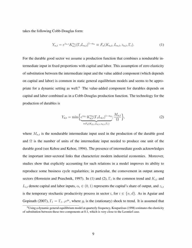
By inspecting Figure 5, we observe that the financial friction does not seem to be nearly

as important in the case of a temporary shock to durables’ production. The reason for this is

that durables represent a relatively small fraction of total output. Therefore, this shock does

not cause output to deviate as much from its steady state and, consequently, the borrowing

premium does not move as much either as in the case of a transitory nondurable shock.

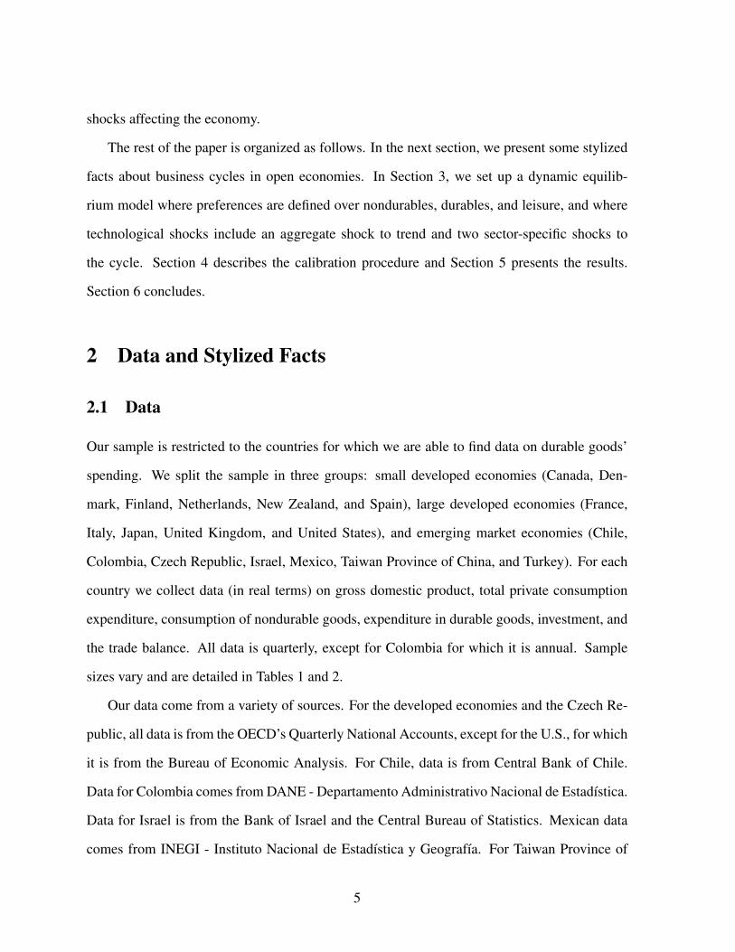
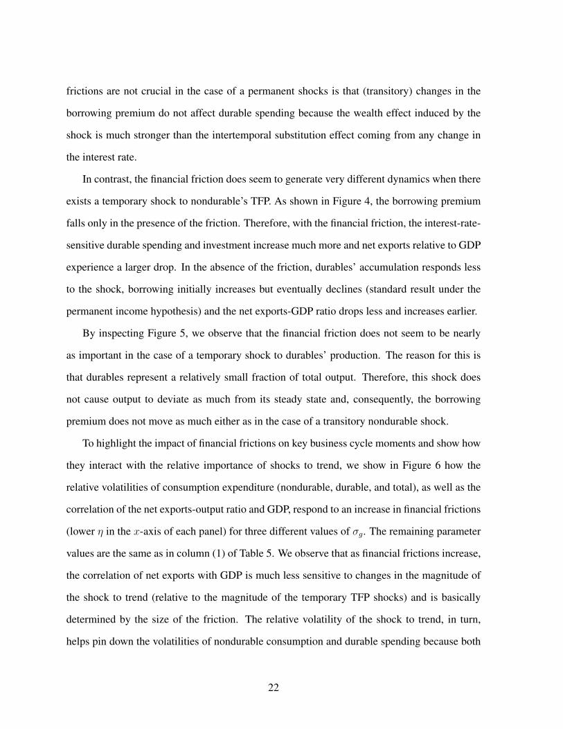
To highlight the impact of financial frictions on key business cycle moments and show how

they interact with the relative importance of shocks to trend, we show in Figure 6 how the

relative volatilities of consumption expenditure (nondurable, durable, and total), as well as the

correlation of the net exports-output ratio and GDP, respond to an increase in financial frictions

(lower η in the x-axis of each panel) for three different values of σg. The remaining parameter

values are the same as in column (1) of Table 5. We observe that as financial frictions increase,

the correlation of net exports with GDP is much less sensitive to changes in the magnitude of

the shock to trend (relative to the magnitude of the temporary TFP shocks) and is basically

determined by the size of the friction. The relative volatility of the shock to trend, in turn,

helps pin down the volatilities of nondurable consumption and durable spending because both

22

expenditures vary with σg for any level of η.

5.3 Robustness

Uribe and Yue (2006) argue that other shocks to the interest rate, independent of income, are

more important to explain the movements of country interest rate premia. For this reason we

modify (16) by adding an orthogonal shock to the borrowing premium, εb,19 with variance σ2b .

We then try to match the volatility of the borrowing premium as well. In this case, according

to the results presented in column (5), we are not able to exactly match the seven moments.

The overall quality of fit, however, remains almost the same and the estimate for σb is zero. In

fact, the results column (5) can be seen as an overdetermined version of the estimation results

presented in column (4). We interpret this result as evidence of the existence of other types

of financial frictions in emerging economies but which are not necessarily unrelated to the

induced country risk.

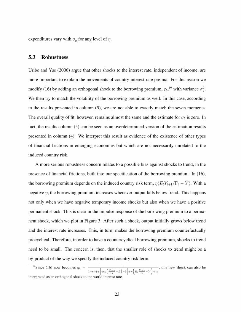
A more serious robustness concern relates to a possible bias against shocks to trend, in the

presence of financial frictions, built into our specification of the borrowing premium. In (16),

the borrowing premium depends on the induced country risk term, η(EtYt+1/Γt − Y ). With a

negative η, the borrowing premium increases whenever output falls below trend. This happens

not only when we have negative temporary income shocks but also when we have a positive

permanent shock. This is clear in the impulse response of the borrowing premium to a perma-

nent shock, which we plot in Figure 3. After such a shock, output initially grows below trend

and the interest rate increases. This, in turn, makes the borrowing premium counterfactually

procyclical. Therefore, in order to have a countercyclical borrowing premium, shocks to trend

need to be small. The concern is, then, that the smaller role of shocks to trend might be a

by-product of the way we specify the induced country risk term.

19Since (16) now becomes qt = 1

1+r∗+χ

[exp(

Bt+1Γt

−B)−1

]+η

(Et

Yt+1Γt

−Y)

+εb

, this new shock can also be

interpreted as an orthogonal shock to the world interest rate.

23

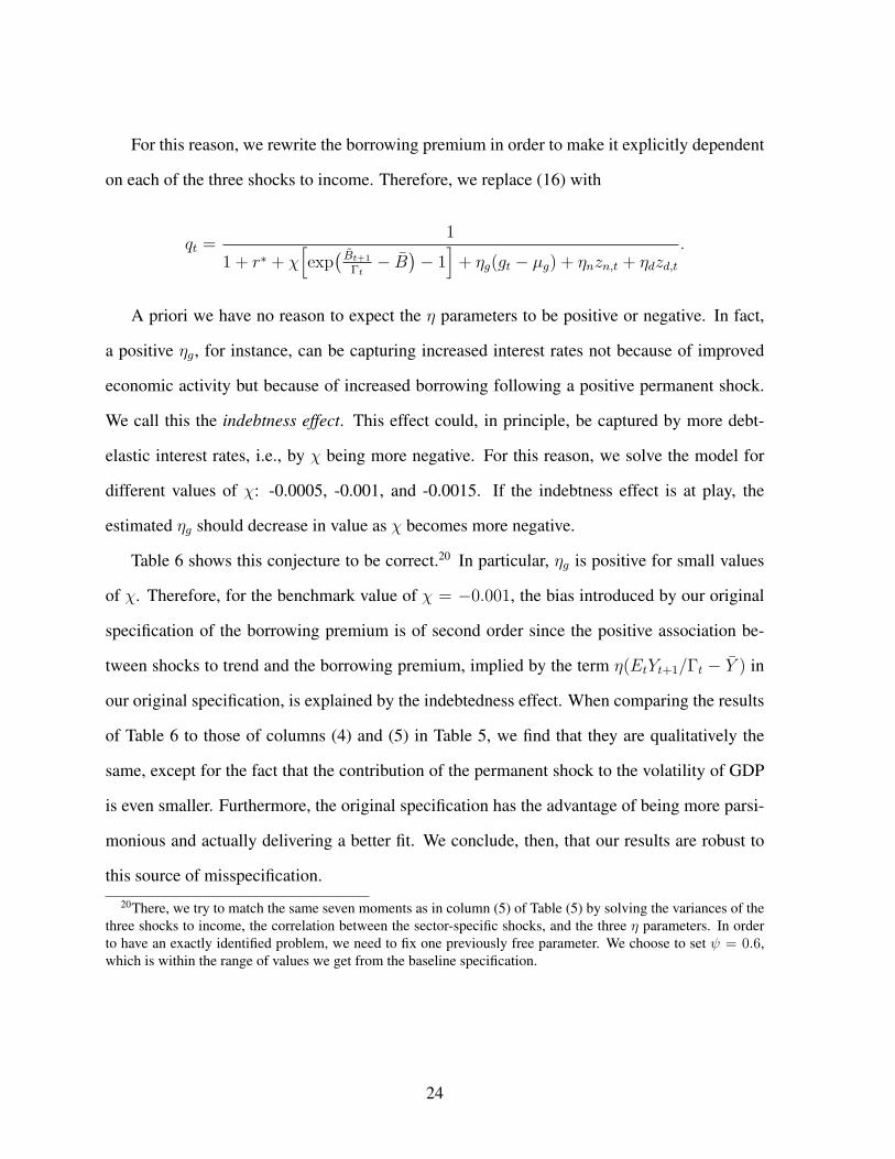
For this reason, we rewrite the borrowing premium in order to make it explicitly dependent

on each of the three shocks to income. Therefore, we replace (16) with

qt =1

1 + r∗ + χ[exp(Bt+1

Γt− B

)− 1]

+ ηg(gt − µg) + ηnzn,t + ηdzd,t.

A priori we have no reason to expect the η parameters to be positive or negative. In fact,

a positive ηg, for instance, can be capturing increased interest rates not because of improved

economic activity but because of increased borrowing following a positive permanent shock.

We call this the indebtness effect. This effect could, in principle, be captured by more debt-

elastic interest rates, i.e., by χ being more negative. For this reason, we solve the model for

different values of χ: -0.0005, -0.001, and -0.0015. If the indebtness effect is at play, the

estimated ηg should decrease in value as χ becomes more negative.

Table 6 shows this conjecture to be correct.20 In particular, ηg is positive for small values

of χ. Therefore, for the benchmark value of χ = −0.001, the bias introduced by our original

specification of the borrowing premium is of second order since the positive association be-

tween shocks to trend and the borrowing premium, implied by the term η(EtYt+1/Γt − Y ) in

our original specification, is explained by the indebtedness effect. When comparing the results

of Table 6 to those of columns (4) and (5) in Table 5, we find that they are qualitatively the

same, except for the fact that the contribution of the permanent shock to the volatility of GDP

is even smaller. Furthermore, the original specification has the advantage of being more parsi-

monious and actually delivering a better fit. We conclude, then, that our results are robust to

this source of misspecification.

20There, we try to match the same seven moments as in column (5) of Table (5) by solving the variances of thethree shocks to income, the correlation between the sector-specific shocks, and the three η parameters. In orderto have an exactly identified problem, we need to fix one previously free parameter. We choose to set ψ = 0.6,which is within the range of values we get from the baseline specification.

24

6 Conclusions

This paper presents a small open economy neoclassical growth model with consumer durables,

nondurable goods, shocks to the trend, and temporary sector-specific shocks. We calibrate the

model to the Mexican economy as representative of an emerging market. We find that financial

frictions in the form of a countercyclical country risk premium play an essential role in ex-

plaining a few empirical facts that characterize cyclical fluctuations in developing economies.

Namely, financial frictions are important to explain a strongly countercyclical trade balance,

and a countercyclical and very volatile borrowing premium.

Our result is in line with Neumeyer and Perri’s (2005) finding. The main difference, how-

ever, is that we do not need to introduce any friction on the firm side and exploit only the nature

of durables accumulation to achieve the desired magnification effect on spending. This result

is also consistent with and reinforces that of Garcıa-Cicco et al. (2010). Our paper, however,

stresses the interaction of durables expenditure (not considered by Garcıa-Cicco et al.) with

financial frictions.

Our results indicate that shocks to trend are somewhat relevant in explaining output and

consumption fluctuations in developing countries. These shocks, however, do not appear to

be the main source of economic fluctuation in emerging economies. The simulations seem to

show, though, that some additional work needs to be done in terms of matching some moments,

namely the volatility of investment.

A natural extension to this paper is to consider other types of shocks. For instance, exoge-

nous shocks to the borrowing premium when durables and nondurables are present should be

considered as a complementary explanation, as the work by Uribe and Yue (2006), Fernandez-

Villaverde et al. (2009) and Gruss and Mertens (2009) seems to suggest. We find that orthog-

onal shocks to the interest rate do not seem to be important to match business cycle moments

in emerging markets. We feel, however, that other types of shocks to the borrowing premium

may play a role and that more work is needed.

25

Another possibility for future research should consider exploring the importance of other

types of financial frictions and external shocks in explaining the properties of business cycles

in emerging markets. For example, we can think of shocks to external wealth which interact

with domestic spending in a variety of ways. One straightforward channel is to see how these

shocks trigger a portfolio rebalancing and cause foreign investors to sell out assets in emerging

markets. This in turn depresses domestic asset prices and lowers permanent income thereby

affecting consumption of both durables and nondurables.

An alternative driving force to be considered, under the presence of durable goods, comes

from shocks to the terms of trade. Many emerging economies are fundamentally producers

of commodities and the prices of many commodities, by their nature, are subject to regime

switching. Consider, for example, an increase in the variance of the terms of trade. As external

income becomes more volatile, default incentives get smaller and, as a consequence, foreign

debt conditions endogenously improve. On the one hand, this allows for smoother consumption

of nondurables, but on the other hand, the purchase of durables may react as households want

to take advance of better borrowing conditions. As a consequence, this type of shocks may

imply a high volatility in the purchase of durable goods and a relatively small volatility of

consumption of non-durables with respect to income volatility. This extension would also

be important in adding micro-foundations to the borrowing premium within a business cycle

model, an important avenue for future research.

26

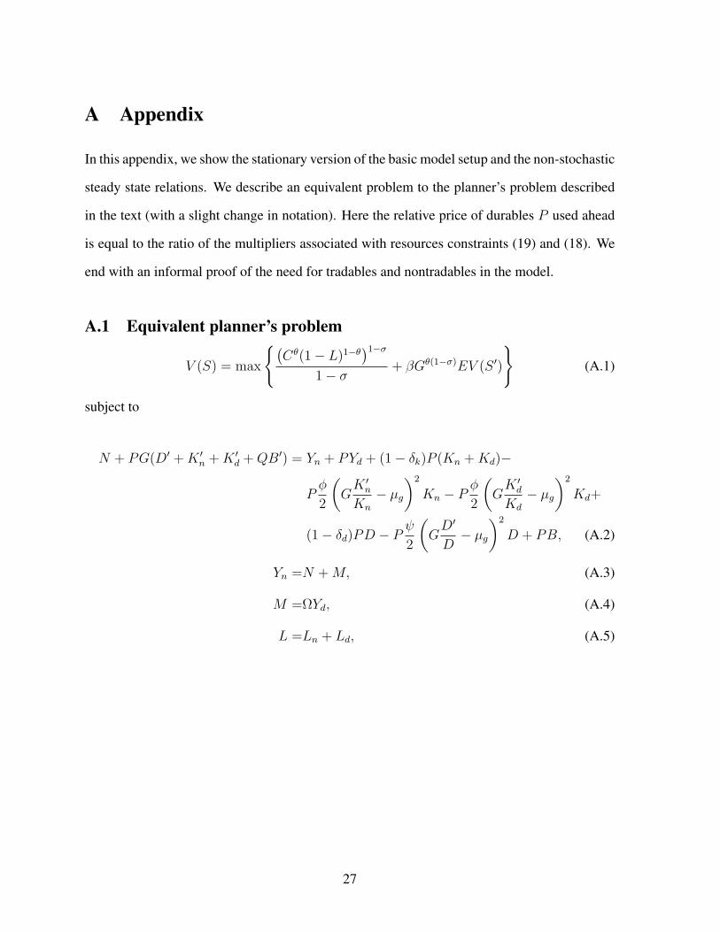
A Appendix

In this appendix, we show the stationary version of the basic model setup and the non-stochastic

steady state relations. We describe an equivalent problem to the planner’s problem described

in the text (with a slight change in notation). Here the relative price of durables P used ahead

is equal to the ratio of the multipliers associated with resources constraints (19) and (18). We

end with an informal proof of the need for tradables and nontradables in the model.

A.1 Equivalent planner’s problem

V (S) = max

(Cθ(1− L)1−θ)1−σ

1− σ+ βGθ(1−σ)EV (S ′)

(A.1)

subject to

N + PG(D′ +K ′n +K ′d +QB′) = Yn + PYd + (1− δk)P (Kn +Kd)−

Pφ

2

(GK ′nKn

− µg)2

Kn − Pφ

2

(GK ′dKd

− µg)2

Kd+

(1− δd)PD − Pψ

2

(GD′

D− µg

)2

D + PB, (A.2)

Yn =N +M, (A.3)

M =ΩYd, (A.4)

L =Ln + Ld, (A.5)

27

with

C ≡(µN−γ + (1− µ)D−γ

)− 1γ , (A.6)

L ≤ 1, (A.7)

Li ≥ 0, i ∈ n, d (A.8)

Ki ≥ 0, i ∈ n, d (A.9)

Q =(1 + r∗ + χ(exp(B′ − B)− 1) + η(EY ′ − Y )

)−1, (A.10)

Yn = ZnKαnn (GLn)1−αn , (A.11)

Yd = ZdKαdd (GLd)

1−αd , (A.12)

lnG′ = (1− ρg) lnµg + ρg lnG+ εg, (A.13)

lnZ ′n = ρn lnZn + εn, (A.14)

lnZ ′d = ρd lnZd + εd. (A.15)

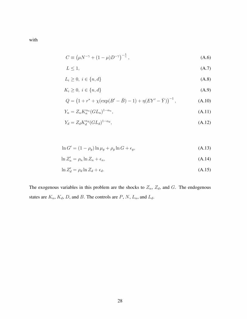
The exogenous variables in this problem are the shocks to Zn, Zd, and G. The endogenous

states are Kn, Kd, D, and B. The controls are P , N , Ln, and Ld.

28

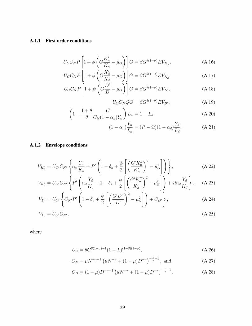
A.1.1 First order conditions

UCCNP

[1 + φ

(GK ′nKn

− µG)]

G = βGθ(1−σ)EVK′n , (A.16)

UCCNP

[1 + φ

(GK ′dKd

− µG)]

G = βGθ(1−σ)EVK′d , (A.17)

UCCNP

[1 + ψ

(GD′

D− µG

)]G = βGθ(1−σ)EVD′ , (A.18)

UCCNQG = βGθ(1−σ)EVB′ , (A.19)(1 +

1 + θ

θ

C

CN(1− αn)Yn

)Ln = 1− Ld, (A.20)

(1− αn)YnLn

= (P − Ω)(1− αd)YdLd. (A.21)

A.1.2 Envelope conditions

VK′n = UC′CN ′

αn

YnKn

+ P ′

(1− δk +

φ

2

[(G′K ′′nK ′n

)2

− µ2G

]), (A.22)

VK′d = UC′CN ′

P ′

(αdYdKd

+ 1− δk +φ

2

[(G′K ′′dK ′d

)2

− µ2G

])+ Ωαd

YdKd

, (A.23)

VD′ = UC′

CN ′P

′

(1− δd +

ψ

2

[(G′D′′

D′

)2

− µ2G

])+ CD′

, (A.24)

VB′ = UC′CN ′ , (A.25)

where

UC = θCθ(1−σ)−1(1− L)(1−θ)(1−σ), (A.26)

CN = µN−γ−1(µN−γ + (1− µ)D−γ

)− 1γ−1, and (A.27)

CD = (1− µ)D−γ−1(µN−γ + (1− µ)D−γ

)− 1γ−1. (A.28)

29

A.2 Steady-state relationships

The steady state variables are: Q, P , Ln, Ld, Kn, Kd, Yn, Yd, N , and D. The steady state is

defined by the following relationships:

Q = βµθ(1−σ)−1g , (A.29)

D =

((1− µ)Q

µP(1− Q(1− δd)

)) 11+γ

N , (A.30)

1− Ld =

(1 +

1− θθ

C

CN(1− αn)Yn

)Ln, (A.31)

(1− αn)YnLn

= (1− αd)PYdLd, (A.32)

αnYnKn

=P (1− (1− δk)Q)

Q, (A.33)

αdYdKd

=P − Ω

P

1− (1− δk)QQ

, (A.34)

Yn = Kαnn (µgLn)1−αn , (A.35)

Yd = Kαdd (µgLd)

1−αd , (A.36)

N = Yn + (P − Ω)Yd + P (1− δk − µg)(Kn + Kd+

P (1− δd − µg)D + P (1− Qµg)B, (A.37)

Yn = N + ΩYd. (A.38)

A.3 Tradability assumption

In this appendix we argue why we need to make the assumption that one good must be non-

tradable. We can do this informally by looking at the steady-state conditions above. In par-

ticular, consider equations (A.32)-(A.34). From the assumption of Cobb-Douglas technology,

both Yi/Li and Yi/Ki are functions of Ki/Li.

Let us argue by contradiction. Let both goods be tradable and the economy be in the

30

deterministic steady state. In this case, P is exogenously given because of our small economy

assumption. Q is given exogenously for the same reason. Therefore, the capital-labor ratios

Ki/Li, i ∈ n, d, are pinned down by equations (A.33) and (A.34). As a result, both the

LHS and RHS of equation (A.32) are given. They only depend on parameters and exogenous

variables P and Q. Clearly, they need not be equal and, thus, the economy may not be at the

deterministic steady state.

31

References

Aguiar, M. and G. Gopinath (2007). Emerging market business cycles: The cycle is the trend.

Journal of Political Economy 115(1), 69–102.

Baxter, M. (1996). Are consumer durables important for business cycles? Review of Economics

and Statistics 78(1), 147–155.

Boz, E., C. Daude, and C. B. Durdu (2008). Emerging market business cycles revisited: Learn-

ing about the trend. International Finance Discussion Paper 927, Federal Reserve Board.

Caballero, R. J. (1993). Durable goods: An explanation for their slow adjustment. Journal of

Political Economy 101(2), 351–384.

De Gregorio, J., P. E. Guidotti, and C. A. Vegh (1998). Inflation stabilisation and the consump-

tion of durable goods. Economic Journal 108(446), 105–131.

De Resende, C. (2006). Endogenous borrowing constraints and consumption volatility in a

small open economy. Working Paper 06-37, Bank of Canada.

Eaton, J. and M. Gersovitz (1981). Debt with potential repudiation: Theoretical and empirical

analysis. Review of Economic Studies 48(2), 289–309.

Engel, C. and J. Wang (2011). International trade in durable goods: Understanding volatility,

cyclicality, and elasticities. Journal of International Economics 83(1), 37–52.

Fernandez-Villaverde, J., P. A. Guerron-Quintana, J. Rubio-Ramırez, and M. Uribe (2009).

Risk matters: The real effects of volatility shocks. Working Paper 14875, National Bureau

of Economic Research.

Galı, J. (1993). Variability of durable and nondurable consumption: Evidence for six O.E.C.D.

countries. Review of Economics and Statistics 75(3), 418–428.

32

Garcıa-Cicco, J., R. Pancrazi, and M. Uribe (2010). Real business cycles in emerging coun-

tries? American Economic Review 100(5), 2510–31.

Gomes, J. F., L. Kogan, and M. Yogo (2009). Durability of output and expected stock returns.

Journal of Political Economy 117(5), 941–986.

Gruss, B. and K. Mertens (2009). Regime switching interest rates and fluctuations in emerging

markets. Economics Working Paper ECO2009/22, European University Institute.

Hornstein, A. and J. Praschnik (1997). Intermediate inputs and sectoral comovement in the

business cycle. Journal of Monetary Economics 40(3), 573–595.

Kehoe, P. J. and T. J. Kehoe (1994). A primer on static applied general equilibrium models.

Federal Reserve Bank of Minneapolis Quarterly Review 18(1), 2–16.

Kouparitsas, M. (1998). Dynamic trade liberalization analysis: Steady state, transitional and

inter-industry effects. Working Paper WP-98-15, Federal Reserve Bank of Chicago.

Mendoza, E. G. (1991). Real business cycles in a small open economy. American Economic

Review 81(4), 797–818.

Neumeyer, P. A. and F. Perri (2005). Business cycles in emerging economies: The role of

interest rates. Journal of Monetary Economics 52(2), 345–380.

Ogaki, M. and C. M. Reinhart (1998). Measuring intertemporal substitution: The role of

durable goods. Journal of Political Economy 106(5), 1078–1098.

Restrepo-Echevarria, P. (2008). Business cycles in developing vs. developed countries: The

importance of the informal economy. Working paper, UCLA.

Rosenzweig, M. R. and K. I. Wolpin (1993). Credit market constraints, consumption smooth-

ing, and the accumulation of durable production assets in low-income countries: Investments

in bullocks in india. Journal of Political Economy 101(2), 223–244.

33

Schmitt-Grohe, S. and M. Uribe (2003). Closing small open economy models. Journal of

International Economics 61(1), 163–185.

Uribe, M. and V. Z. Yue (2006). Country spreads and emerging countries: Who drives whom?

Journal of International Economics 69(1), 6–36.

34

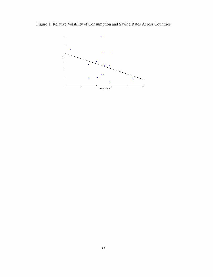
Figure 1: Relative Volatility of Consumption and Saving Rates Across Countries

35

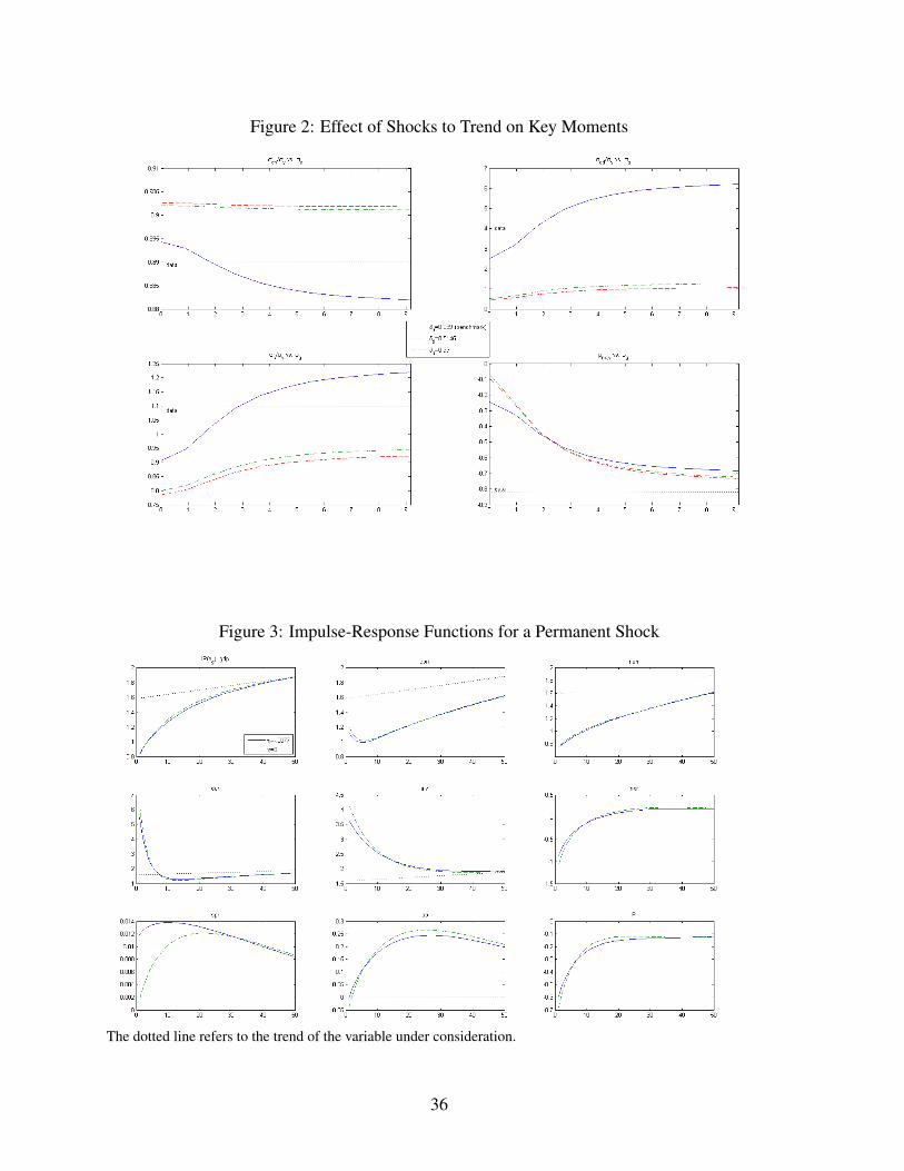
Figure 2: Effect of Shocks to Trend on Key Moments

Figure 3: Impulse-Response Functions for a Permanent Shock

The dotted line refers to the trend of the variable under consideration.

36

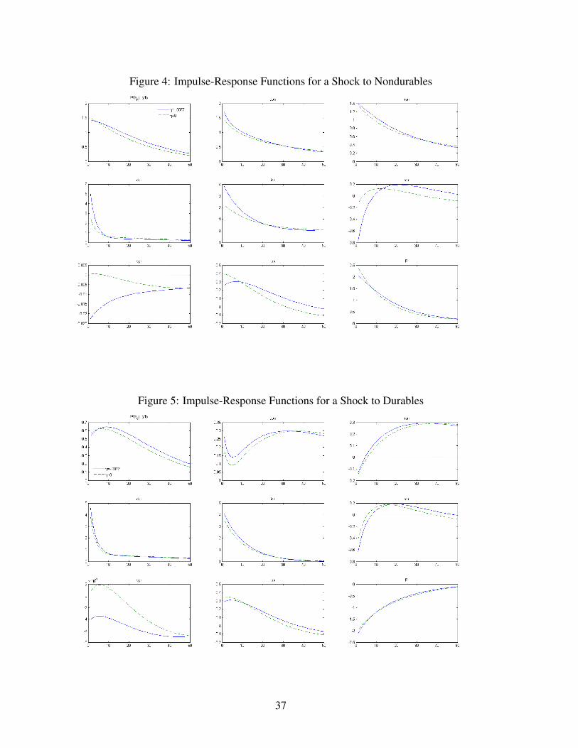
Figure 4: Impulse-Response Functions for a Shock to Nondurables

Figure 5: Impulse-Response Functions for a Shock to Durables

37

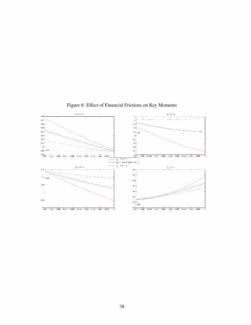
Figure 6: Effect of Financial Frictions on Key Moments

38

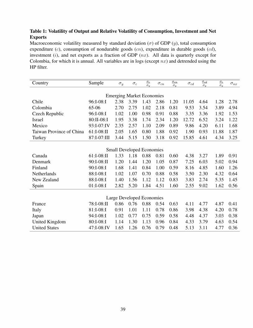
Table 1: Volatility of Output and Relative Volatility of Consumption, Investment and NetExportsMacroeconomic volatility measured by standard deviation (σ) of GDP (y), total consumptionexpenditure (c), consumption of nondurable goods (cn), expenditure in durable goods (cd),investment (i), and net exports as a fraction of GDP (nx). All data is quarterly except forColombia, for which it is annual. All variables are in logs (except nx) and detrended using theHP filter.

Country Sample σy σcσcσy

σcnσcnσy

σcdσcdσy

σiσy

σnx

Emerging Market EconomiesChile 96:I-08:I 2.38 3.39 1.43 2.86 1.20 11.05 4.64 1.28 2.78Colombia 65-06 2.70 2.75 1.02 2.18 0.81 9.53 3.54 3.89 4.94Czech Republic 96:I-08:I 1.02 1.00 0.98 0.91 0.88 3.35 3.36 1.92 1.53Israel 80:II-08:I 1.95 3.38 1.74 2.34 1.20 12.72 6.52 3.24 1.22Mexico 93:I-07:IV 2.35 2.57 1.10 2.09 0.89 9.86 4.20 6.11 1.68Taiwan Province of China 61:I-08:II 2.05 1.65 0.80 1.88 0.92 1.90 0.93 11.88 1.87Turkey 87:I-07:III 3.44 5.15 1.50 3.18 0.92 15.85 4.61 4.34 3.25

Small Developed EconomiesCanada 61:I-08:II 1.33 1.18 0.88 0.81 0.60 4.38 3.27 1.89 0.91Denmark 90:I-08:II 1.20 1.44 1.20 1.05 0.87 7.25 6.03 5.02 0.94Finland 90:I-08:I 1.68 1.41 0.84 1.00 0.59 8.16 4.85 1.60 1.26Netherlands 88:I-08:I 1.02 1.07 0.70 0.88 0.58 3.50 2.30 4.32 0.64New Zealand 88:I-08:I 1.40 1.56 1.12 1.12 0.83 3.83 2.74 5.35 1.45Spain 01:I-08:I 2.82 5.20 1.84 4.51 1.60 2.55 9.02 1.62 0.56

Large Developed EconomiesFrance 78:I-08:II 0.86 0.76 0.88 0.54 0.63 4.11 4.77 4.87 0.41Italy 81:I-08:I 0.91 1.01 1.11 0.78 0.86 3.98 4.38 4.20 0.78Japan 94:I-08:I 1.02 0.77 0.75 0.59 0.58 4.48 4.37 3.03 0.38United Kingdom 80:I-08:I 1.14 1.30 1.13 0.96 0.84 4.33 3.79 4.63 0.54United States 47:I-08:IV 1.65 1.26 0.76 0.79 0.48 5.13 3.11 4.77 0.36

39

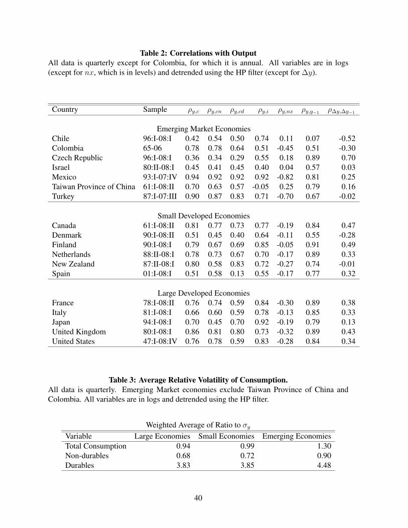
Table 2: Correlations with OutputAll data is quarterly except for Colombia, for which it is annual. All variables are in logs(except for nx, which is in levels) and detrended using the HP filter (except for ∆y).

Country Sample ρy,c ρy,cn ρy,cd ρy,i ρy,nx ρy,y−1 ρ∆y,∆y−1

Emerging Market EconomiesChile 96:I-08:I 0.42 0.54 0.50 0.74 0.11 0.07 -0.52Colombia 65-06 0.78 0.78 0.64 0.51 -0.45 0.51 -0.30Czech Republic 96:I-08:I 0.36 0.34 0.29 0.55 0.18 0.89 0.70Israel 80:II-08:I 0.45 0.41 0.45 0.40 0.04 0.57 0.03Mexico 93:I-07:IV 0.94 0.92 0.92 0.92 -0.82 0.81 0.25Taiwan Province of China 61:I-08:II 0.70 0.63 0.57 -0.05 0.25 0.79 0.16Turkey 87:I-07:III 0.90 0.87 0.83 0.71 -0.70 0.67 -0.02

Small Developed EconomiesCanada 61:I-08:II 0.81 0.77 0.73 0.77 -0.19 0.84 0.47Denmark 90:I-08:II 0.51 0.45 0.40 0.64 -0.11 0.55 -0.28Finland 90:I-08:I 0.79 0.67 0.69 0.85 -0.05 0.91 0.49Netherlands 88:II-08:I 0.78 0.73 0.67 0.70 -0.17 0.89 0.33New Zealand 87:II-08:I 0.80 0.58 0.83 0.72 -0.27 0.74 -0.01Spain 01:I-08:I 0.51 0.58 0.13 0.55 -0.17 0.77 0.32

Large Developed EconomiesFrance 78:I-08:II 0.76 0.74 0.59 0.84 -0.30 0.89 0.38Italy 81:I-08:I 0.66 0.60 0.59 0.78 -0.13 0.85 0.33Japan 94:I-08:I 0.70 0.45 0.70 0.92 -0.19 0.79 0.13United Kingdom 80:I-08:I 0.86 0.81 0.80 0.73 -0.32 0.89 0.43United States 47:I-08:IV 0.76 0.78 0.59 0.83 -0.28 0.84 0.34

Table 3: Average Relative Volatility of Consumption.All data is quarterly. Emerging Market economies exclude Taiwan Province of China andColombia. All variables are in logs and detrended using the HP filter.

Weighted Average of Ratio to σyVariable Large Economies Small Economies Emerging EconomiesTotal Consumption 0.94 0.99 1.30Non-durables 0.68 0.72 0.90Durables 3.83 3.85 4.48

40

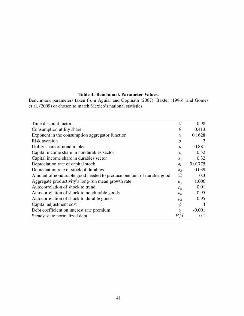
Table 4: Benchmark Parameter Values.Benchmark parameters taken from Aguiar and Gopinath (2007), Baxter (1996), and Gomeset al. (2009) or chosen to match Mexico’s national statistics.

Time discount factor β 0.98Consumption utility share θ 0.413Exponent in the consumption aggregator function γ 0.1628Risk aversion σ 2Utility share of nondurables µ 0.881Capital income share in nondurables sector αn 0.52Capital income share in durables sector αd 0.32Depreciation rate of capital stock δk 0.01775Depreciation rate of stock of durables δd 0.039Amount of nondurable good needed to produce one unit of durable good Ω 0.3Aggregate productivity’s long-run mean growth rate µg 1.006Autocorrelation of shock to trend ρg 0.01Autocorrelation of shock to nondurable goods ρn 0.95Autocorrelation of shock to durable goods ρd 0.95Capital adjustment cost φ 4Debt coefficient on interest rate premium χ -0.001Steady-state normalized debt B/Y -0.1

41

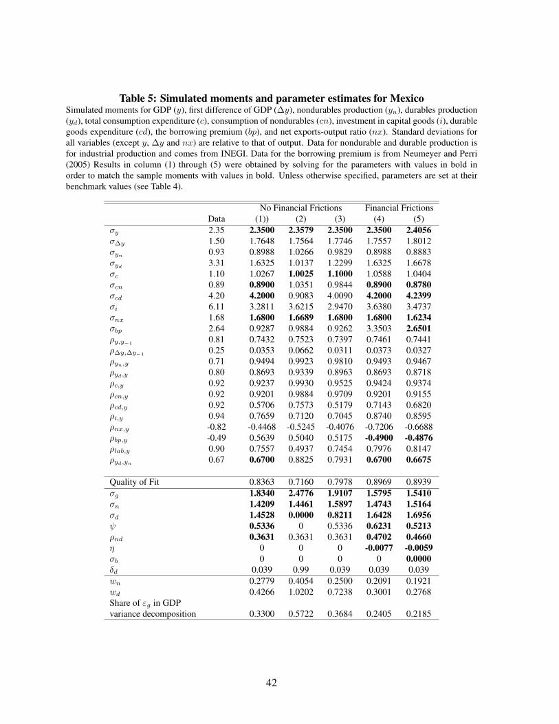
Table 5: Simulated moments and parameter estimates for MexicoSimulated moments for GDP (y), first difference of GDP (∆y), nondurables production (yn), durables production(yd), total consumption expenditure (c), consumption of nondurables (cn), investment in capital goods (i), durablegoods expenditure (cd), the borrowing premium (bp), and net exports-output ratio (nx). Standard deviations forall variables (except y, ∆y and nx) are relative to that of output. Data for nondurable and durable production isfor industrial production and comes from INEGI. Data for the borrowing premium is from Neumeyer and Perri(2005) Results in column (1) through (5) were obtained by solving for the parameters with values in bold inorder to match the sample moments with values in bold. Unless otherwise specified, parameters are set at theirbenchmark values (see Table 4).

No Financial Frictions Financial FrictionsData (1)) (2) (3) (4) (5)

σy 2.35 2.3500 2.3579 2.3500 2.3500 2.4056σ∆y 1.50 1.7648 1.7564 1.7746 1.7557 1.8012σyn 0.93 0.8988 1.0266 0.9829 0.8988 0.8883σyd

3.31 1.6325 1.0137 1.2299 1.6325 1.6678σc 1.10 1.0267 1.0025 1.1000 1.0588 1.0404σcn 0.89 0.8900 1.0351 0.9844 0.8900 0.8780σcd 4.20 4.2000 0.9083 4.0090 4.2000 4.2399σi 6.11 3.2811 3.6215 2.9470 3.6380 3.4737σnx 1.68 1.6800 1.6689 1.6800 1.6800 1.6234σbp 2.64 0.9287 0.9884 0.9262 3.3503 2.6501ρy,y−1 0.81 0.7432 0.7523 0.7397 0.7461 0.7441ρ∆y,∆y−1 0.25 0.0353 0.0662 0.0311 0.0373 0.0327ρyn,y 0.71 0.9494 0.9923 0.9810 0.9493 0.9467ρyd,y 0.80 0.8693 0.9339 0.8963 0.8693 0.8718ρc,y 0.92 0.9237 0.9930 0.9525 0.9424 0.9374ρcn,y 0.92 0.9201 0.9884 0.9709 0.9201 0.9155ρcd,y 0.92 0.5706 0.7573 0.5179 0.7143 0.6820ρi,y 0.94 0.7659 0.7120 0.7045 0.8740 0.8595ρnx,y -0.82 -0.4468 -0.5245 -0.4076 -0.7206 -0.6688ρbp,y -0.49 0.5639 0.5040 0.5175 -0.4900 -0.4876ρlab,y 0.90 0.7557 0.4937 0.7454 0.7976 0.8147ρyd,yn

0.67 0.6700 0.8825 0.7931 0.6700 0.6675

Quality of Fit 0.8363 0.7160 0.7978 0.8969 0.8939σg 1.8340 2.4776 1.9107 1.5795 1.5410σn 1.4209 1.4461 1.5897 1.4743 1.5164σd 1.4528 0.0000 0.8211 1.6428 1.6956ψ 0.5336 0 0.5336 0.6231 0.5213ρnd 0.3631 0.3631 0.3631 0.4702 0.4660η 0 0 0 -0.0077 -0.0059σb 0 0 0 0 0.0000δd 0.039 0.99 0.039 0.039 0.039wn 0.2779 0.4054 0.2500 0.2091 0.1921wd 0.4266 1.0202 0.7238 0.3001 0.2768Share of εg in GDPvariance decomposition 0.3300 0.5722 0.3684 0.2405 0.2185

42

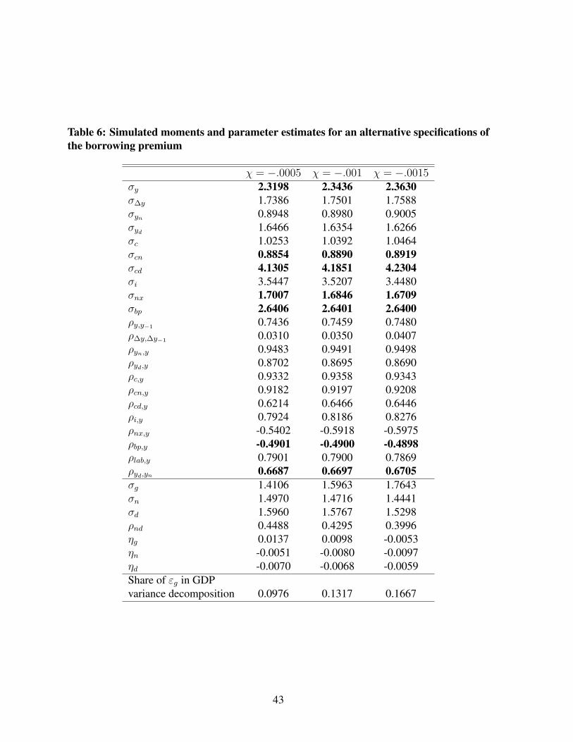
Table 6: Simulated moments and parameter estimates for an alternative specifications ofthe borrowing premium

χ = −.0005 χ = −.001 χ = −.0015σy 2.3198 2.3436 2.3630σ∆y 1.7386 1.7501 1.7588σyn 0.8948 0.8980 0.9005σyd 1.6466 1.6354 1.6266σc 1.0253 1.0392 1.0464σcn 0.8854 0.8890 0.8919σcd 4.1305 4.1851 4.2304σi 3.5447 3.5207 3.4480σnx 1.7007 1.6846 1.6709σbp 2.6406 2.6401 2.6400ρy,y−1 0.7436 0.7459 0.7480ρ∆y,∆y−1 0.0310 0.0350 0.0407ρyn,y 0.9483 0.9491 0.9498ρyd,y 0.8702 0.8695 0.8690ρc,y 0.9332 0.9358 0.9343ρcn,y 0.9182 0.9197 0.9208ρcd,y 0.6214 0.6466 0.6446ρi,y 0.7924 0.8186 0.8276ρnx,y -0.5402 -0.5918 -0.5975ρbp,y -0.4901 -0.4900 -0.4898ρlab,y 0.7901 0.7900 0.7869ρyd,yn 0.6687 0.6697 0.6705σg 1.4106 1.5963 1.7643σn 1.4970 1.4716 1.4441σd 1.5960 1.5767 1.5298ρnd 0.4488 0.4295 0.3996ηg 0.0137 0.0098 -0.0053ηn -0.0051 -0.0080 -0.0097ηd -0.0070 -0.0068 -0.0059Share of εg in GDPvariance decomposition 0.0976 0.1317 0.1667

43