Embed Size (px)
Citation preview
ANY OPINIONS EXPRESSED ARE THOSE OF THE AUTHOR(S) AND NOT NECESSARILY THOSE OF THE SCHOOL OF ECONOMICS & SOCIAL SCIENCES, SMU
Analyzing and Forecasting Business Cycles in a Small Open Economy: A Dynamic Factor Model for Singapore
Hwee Kwan Chow and Keen Meng Choy February 2009
Paper No. 05-2009
Analyzing and Forecasting Business Cycles in a Small Open Economy: A Dynamic Factor Model for Singapore
Hwee Kwan Chow1 and Keen Meng Choy2
Abstract
A dynamic factor model is applied to a large panel dataset of Singapore’s macroeconomic variables and global economic indicators with the initial objective of analyzing business cycles in a small open economy. The empirical results suggest that four common factors are present in the quarterly time series, which can broadly be interpreted as world, regional, electronics and domestic economic cycles. The estimated factor model explains well the observed fluctuations in real economic activity and price inflation, leading us to use it in forecasting Singapore’s business cycles. We find that the forecasts generated by the factors are generally more accurate than the predictions of univariate models and vector autoregressions that employ leading indicators.
Key Words: Business cycle, Dynamic factor model, Forecasting, Singapore
JEL Classification: C32, C33, E32, E37
1School of Economics, Singapore Management University, Singapore; [email protected] 2 Division of Economics, Nanyang Technological University, Singapore; [email protected] The authors would like to thank the Office of Research, Singapore Management University for research grant support, and participants at the 2008 Australasian and Far Eastern Meetings of the Econometric Society for their comments.
1
1 Introduction The analysis of business cycles in small and open economies has always
presented the empirical researcher with particular challenges. A fundamental reason for
this lies in the vulnerability of such economies to the vagaries of international
macroeconomic fluctuations, which accentuate the intrinsic volatility caused by
domestically generated disturbances. Nonetheless, many papers appearing in scholarly
journals are cognizant of the role played by international fluctuations when documenting
the stylized facts of business cycle co-movements in relatively open economies such as
Sweden, Switzerland, New Zealand and Korea (see respectively Englund et al., 1992;
Danthine and Girardin, 1989; Kim et al., 1994; Kim and Choi, 1997). In addition to these
industrialized country studies, Kose, Otrok and Whiteman (2003) successfully used
worldwide, regional and country-specific business cycles to explain the aggregate co-
movements observed in a broad cross-section of countries.
Two articles that examined the nature of economic fluctuations in the small and
newly industrialized economies of Hong Kong and Singapore find that, in line with the
studies cited above, external factors contribute significantly to their internal gyrations
(Leung and Suen, 2001; Choy, 2009). Unfortunately, attempts to include the impact of
international events in business cycle modelling of highly open economies are often
hampered by the need for parsimony. Typically, the problem is approached on an ad hoc
basis, using only a limited number of foreign variables to represent external shocks to the
economy. This is to avoid running into the degrees-of-freedom problem associated with a
loss of efficiency in regression-type models such as single equations, large scale
macroeconometric models and vector autoregressions.
As a remedy, one could consider dynamic factor models that permit the
incorporation of a large number of variables capturing the foreign disturbances which
buffet small and open economies as well as impulses originating from domestic sources.
This class of models is appealing from a theoretical standpoint since it views all
macroeconomic fluctuations as being driven by a small number of common shocks and
an idiosyncratic component that is peculiar to each economic time series—an idea that
was already implicit in Burns and Mitchell’s (1946) early characterization of business
cycles. In spite of the seminal papers by Sargent and Sims (1977) and Stock and Watson
2
(1989), dynamic factor models have only lately been revived for the purpose of
forecasting real economic activity and inflation in the US and larger European countries
(see, inter alia, García-Ferrer and Poncela, 2002; Stock and Watson, 2002b; Forni et al.,
2003; Artis et al., 2005; Schumacher, 2007). However, their use as a tool of business
cycle analysis particularly with respect to small open economies remains relatively
unexplored, even as the statistical techniques and computing power needed to efficiently
exploit the vast amount of information in large panel datasets were developed.
In this paper, we demonstrate the usefulness of a dynamic factor model for the
analysis and prediction of business cycles in an archetypal small open economy with an
empirical application to Singapore. Unlike the earlier work on single factor models by
Stock and Watson (1989) and others aimed at the construction of composite indexes of
economic activity based on a mere handful of coincident indicators, we utilize a large
collection of 177 quarterly time series that includes foreign economic indicators as well as
domestic variables to extract the unobserved factors responsible for macroeconomic
fluctuations. Another difference is that we allow more than one common factor to drive
fluctuations, which is congruent with the assumption that business cycles are caused by
multiple sources of shocks. Moreover, the number of shocks is determined rigorously
using the recent method proposed by Bai and Ng (2007).
It turns out that the bulk of the observed co-variation in the variables under
consideration can be explained with just four common factors, suggesting that the
Singapore macroeconomic data can be approximated by a low-dimensional factor
structure despite its diversity. Although we refrain from imposing identification
assumptions, we surmise that the factors represent world, regional, electronics and
domestic economic cycles through a detailed analysis of their explanatory power for
various time series. Since the estimated factors account very well for the cyclical
fluctuations in real economic activity and general price inflation, we use them next in
short-term forecasting. We generate predictions recursively from a direct multistep
forecasting methodology and compare them with forecasts of univariate and multivariate
time series models. The latter makes use of known leading indicators of the Singapore
economy and could be considered to be a sophisticated competitor to factor models. We
3
find that the factor approach leads to improvements in forecast performance for most of
the variables investigated.
The rest of the paper is structured as follows. Section 2 presents the dynamic
factor model for the Singapore economy, describes its estimation, and outlines the Bai-Ng
test for the number of aggregate shocks in the model. Section 3 describes the panel
dataset employed and its cyclical properties. Section 4 reports the empirical results from
estimating the dynamic factor model and provides plausible interpretations of the latent
factors by relating them to macroeconomic variables. In Section 5, we produce pseudo
out-of-sample predictions of the growth rates in major output and price indicators from the
alternative forecasting models and formally evaluate their relative accuracy. Lastly, the
paper’s conclusions are given in Section 6.
2 The Dynamic Factor Model 2.1 Representation and estimation
Variables cast in a factor analytic representation are characterized by the sum of
two mutually orthogonal and unobservable components: the common component driven
by a small number of factors and the idiosyncratic component driven by variable-specific
shocks. Denoting the size of the cross-sectional panel by N and the length of each time
series by T, let , 1, ,t ,X t = … T be the N-dimensional vector of stationary time series. The
dynamic factor model for these variables is given by:
( )it i t itX L fλ ε= + (1)
for The vector 1, , .i = … N 1q× tf contains the common factors and
0 1( ) si iL Li isLλ λ λ= +
it
λ+ + is an s-th order polynomial in the lag operator that represents
a vector of dynamic factor loadings. In contrast to the exact factor model, the idiosyncratic
disturbance
L
ε is permitted to have limited serial and cross-correlation (see Forni et al.,
2000 and Stock and Watson, 2002b). However, the factors and idiosyncratic errors are
4
assumed to be mutually uncorrelated at all leads and lags—an assumption that is
essential for estimation of the factor model.
The central idea of the factor model as applied to business cycle analysis is that
information in a large dataset can be parsimoniously summarized by a small number of
latent factors i.e. q , each of which could be estimated as a weighted linear
combination of the cycles found in individual variables. In other words, economic
variables are pooled to average out noisy disturbances in the idiosyncratic component
and to extract the cyclical signals in the common component. We assume that the latter
explains the major part of the variation in observed time series regardless of the cross-
sectional dimension. In the dynamic version of the factor analytic model described by
N
(1),
current realizations of variables can be affected by the past values of factors through a
finite distributed lag structure. Further, the dynamic factor model relaxes the assumption
of uncorrelated disturbances required in classical factor analysis by allowing for both
contemporaneous and lagged correlation between the idiosyncratic terms, thereby
accommodating the typical statistical features of macroeconomic data employed in
business cycle analysis and forecasting applications.
For estimation purposes, the model in (1) often reformulated as:
t tX F tε= Λ + (2)
where is an ( ), ,t t t sF f f −′′ ′= … ( )1r q s= + -dimensional vector of stacked common factors
and is now an N matrix of factor loadings. Notice that the r static factors in
consist of current and s lagged values of the q dynamic factors in
Λ r× tF
tf . The key advantage
of this static representation is that principal components analysis can be applied to extract
the common factors from a huge panel of related time series in a computationally
convenient manner. Specifically, the column space spanned by the dynamic factors can
be estimated consistently as jointly by taking principal components of the
covariance matrix of
,N T →∞
tX , provided mild regularity conditions are satisfied (Stock and
5
Watson, 2002b).3 One key condition is that the static factors included in the model has to
be at least equal to their true number, so it is important that a reliable procedure be used
to determine the value of r.
2.2 Determination of the number of factors
Bai and Ng (2007) demonstrated that the dynamic factor in (1) always has the
static factor representation (2) in which the dynamics of are characterized by a VAR. In
the same paper, they showed how the number of dynamic factors, q, can be inferred from
a knowledge of the number of static factors, r. Since some factors in the static model are
dynamically dependent—being lags of the others—it follows that q . This observation
forms the basis of Bai and Ng’s method to determine the value of q, which the authors
interpret as a test for the number of primitive shocks driving macroeconomic fluctuations.
Specifically, q is the reduced rank of the residual covariance matrix for the static factor
VAR, or the number of non-zero eigenvalues associated with it.
tF
r≤
The Bai-Ng procedure consists of two steps. In the first, the static factors are
estimated by principal components analysis and r is consistently selected using one of
the six variants of information criteria developed in their earlier work (Bai and Ng, 2002).
All the criteria are asymptotically equivalent but their small sample properties vary due to
different specifications of the penalty term. The most widely used criterion and one of the
best in terms of performance in simulations is the following:
( )( ) { }(( ) ln , ln min ,N T )IC r V r F r N TNT+⎛ ⎞= + ⎜ ⎟
⎝ ⎠ (3)
( ) ( )2
1 1
1,N T
it i ti t
V r F X FNT = =
= −∑∑ Λ
(4)
The penalty imposed by the second term in (3), which is an increasing function of N and T
as well as the number of factors, serves to counter-balance the minimized residual sum of
3 Stock and Watson (2002a) in fact proved the stronger result that, even if there is parameter instability caused by, say, structural change, the principal component estimates are still consistent because their precision improves with N, thus making it possible to compensate for short panels where T is relatively small.
6
squares by effecting an optimal trade-off between goodness of fit and over-fitting.
Evidently, the criterion can be viewed as an extension of the Akaike information criterion
(AIC) with consideration for the additional cross-sectional dimension to the time series.
In the second step, the principal components estimates of the factors conditional
on the value of r selected are used to fit a VAR model of order p and the least squares
residuals are obtained. As mentioned above, the method to determine q is based on the
estimated eigenvalues of the residual covariance matrix. Let these be denoted as
in descending order. The cumulative contribution of the k-th eigenvalue
is given by:
1 2ˆ ˆ ˆ 0rc c c≥ ≥ ≥ ≥…
122
1
21
ˆˆ
ˆ
rjj k
k rjj
cD
c= +
=
⎛ ⎞⎜ ⎟=⎜ ⎟⎝ ⎠
∑∑
(5)
Assuming that the true number of dynamic factors is q, 0kc = for k . Bai and Ng (2007)
showed that converges asymptotically to zero for k at a rate depending on the
sampling error induced by estimation of the VAR covariance matrix. Hence, for non-
negative m and
q>
ˆkD q≥
0 1 2δ< < , the smallest integer k that satisfies the bounded set
{ }1 12 2ˆ: / min ,kk D m N Tδ δ− −⎡ ⎤< ⎣ ⎦ is the estimated number of dynamic factors in the model.
The large sample property of the test ensures that this value of k will be a consistent
estimate of q as N and T diverge.
3 The Panel Dataset
Singapore has a large and reliable database of macroeconomic variables by the
standards of newly industrialized economies. The national income accounts, in particular,
are very rich in revealing the industry details of the compilation of real GDP by the
production approach. Given this, we broaden our search for the set of cyclical indicators
to be included in the factor model to time series of the quarterly frequency, hence
providing a more comprehensive coverage of the many facets of macroeconomic activity.
Needless to say, monthly data is not excluded from the exercise, although these have to
7
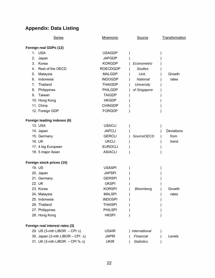
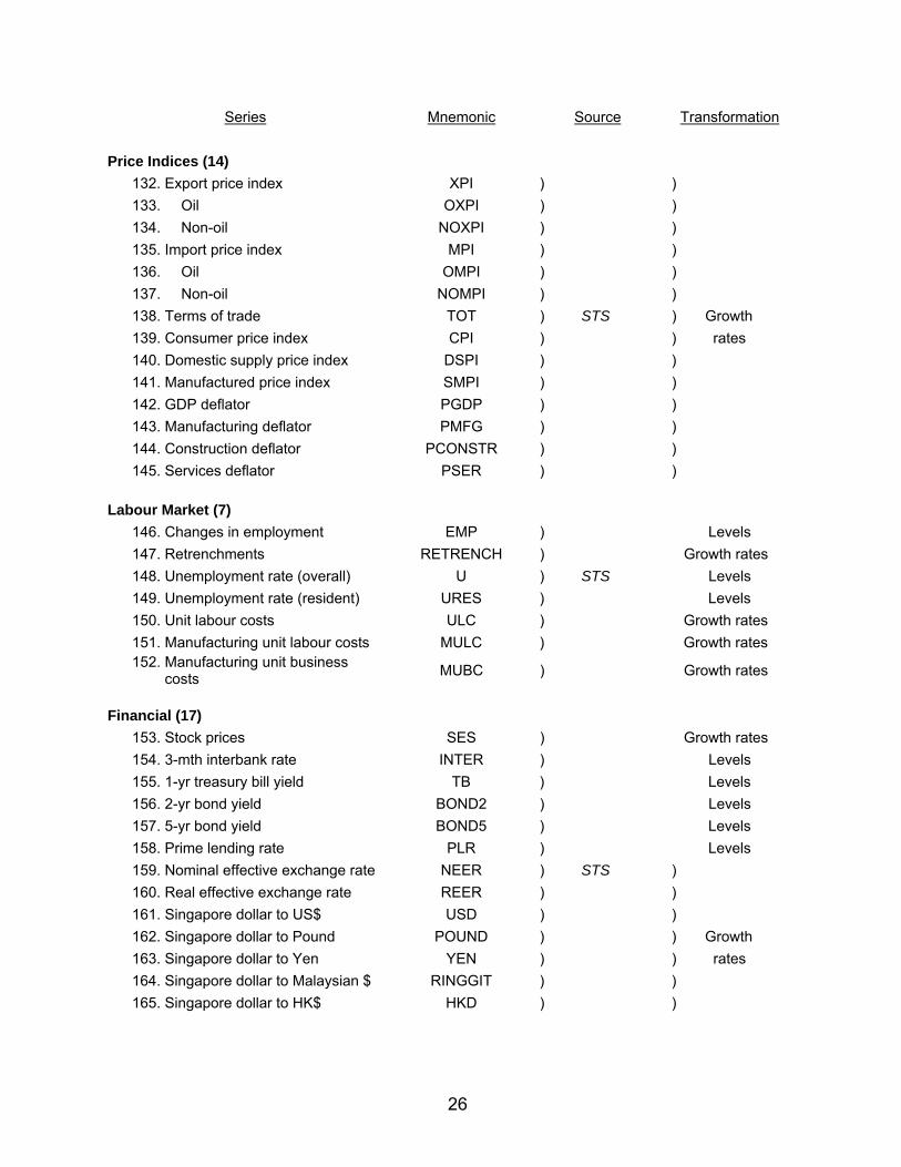
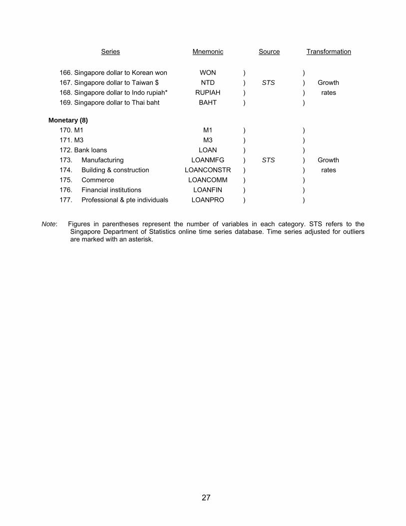
be aggregated or averaged to yield quarterly values. The variables selected are listed in
the appendix.
As our interest is in analyzing and predicting Singapore’s growth cycles, almost all
the variables we work with are transformed into approximate year-on-year (or annualized)
growth rates by taking the fourth differences of their logarithms. In this respect, we depart
from the conventional practice of modelling period-on-period (or quarterly) growth rates
since these are very volatile for a small open economy like Singapore. The only variables
to which the growth rate transformation is not applied and where seasonally adjusted data
are used instead are interest rates, exchange rates, unemployment and business
expectations series.
To avoid overweighting any one series, all raw and transformed variables are
normalized by subtracting their means and dividing by their standard deviations. A visual
inspection of time plots revealed a handful of unusual occurrences during the sample
period from 1993Q1 to 2008Q2 due to the Asian financial crisis of 1997 and the outbreak
of the SARS disease in early 2003. As a robustness measure, the outlying observations
are excluded in the computation of the means and standard deviations of contaminated
series. In view of the fact that Singapore is a major producer of semiconductor products,
the choice of starting date was dictated by the availability of data on electronics time
series, resulting in T = 62. However, the relatively small sample size is compensated by a
large panel that consists of 41 transnational and 136 national indicators, making N = 177.
These series can be loosely grouped as follows:
• Real GDPs of Singapore’s major trading partners and their weighted average (10
countries and one region); composite leading indexes of the US and major
European and Asian economies; foreign stock prices and interest rates
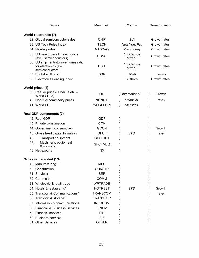
• Global semiconductor sales, US technology cycle index and electronics leading
indicators plus index; world oil price, non-fuel commodity prices and global
consumer prices
8

• Singapore’s real GDP and expenditure components; gross value-added output in
the manufacturing, service and construction sectors
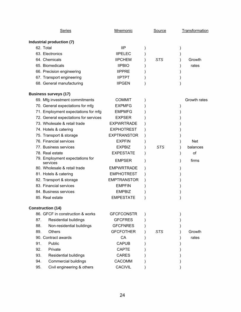
• Industrial production indices; investment commitments and business expectations
surveys; composite leading index
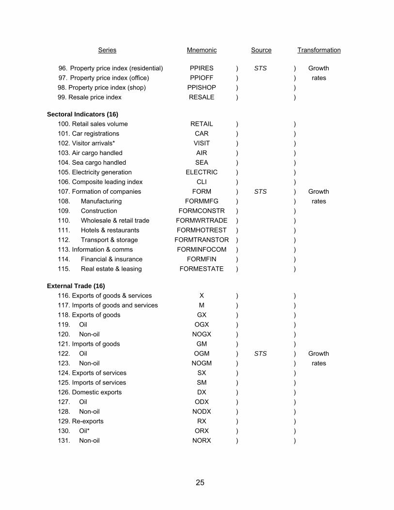
• Construction and housing related series e.g. residential investment, building
contracts awarded and property prices
• Sectoral indicators such as retail sales, new car registrations, tourist arrivals, air
and sea cargo handled, electricity generation and company formations in different
sectors
• Foreign trade series: exports and imports of goods and services, domestic exports
and re-exports disaggregated into oil and non-oil categories
• Export and import price indices; terms of trade; consumer and producer price
indices; GDP and sectoral deflators
• Labour market variables: changes in employment, retrenchments, unemployment
rates, unit labour and business costs
• Financial series such as stock prices, interest rates and exchange rates; monetary
aggregates and bank credit
As noted above, the importance of international and foreign economic indicators
for short-term monitoring of the Singapore economy should not be underestimated, so it is
imperative to consider external series that are known to co-move with—and sometimes
lead—local variables. The time series proven to be leading indicators of business cycles
in Singapore are not limited to foreign composite leading indexes and asset prices, but
include worldwide electronics indicators such as the book-to-bill ratio for semiconductor
9
equipment, US new orders of electronics and the electronics leading index created by
Chow and Choy (2006), which has shown an ability to forecast the global semiconductor
cycle up to six months ahead.
The cyclical properties of the domestic variables are also worth highlighting.
Almost all of them exhibit procyclical or counter-cyclical movements with reference to the
growth cycles in real GDP extracted by a band-pass filter (Choy, 2009). The
demonstrably leading series are business anticipations, company formations, producer
prices, money supply, the nominal exchange rate and the value of construction contracts
awarded (see Chow, 1993 and Chow and Choy, 1995). Some of these indicators are
components of the composite leading index compiled by the Singapore authorities
(Department of Statistics, 2004), which is also included in the dataset.
By contrast, the consumer price level, nominal wages and interest rates lag
economic activity, as do employment and the unemployment rate (Choy, 2009). Finally,
the strongly coincident variables are real GDP, sectoral value-added indicators, industrial
production, non-oil domestic exports, retail sales and electricity generation. Regardless of
a variable’s cyclical timing classification, it can easily be fitted into the very flexible factor
framework by virtue of the lag polynomial in (1). As a result, the inclusion of leading,
coincident and lagging economic indicators in the estimation and forecasting exercises
promises to deliver sharper estimates of the latent factors underlying movements in
Singapore’s output and prices.
4 Analyzing Singapore Business Cycles
Implementing the Bai-Ng information criterion in (3) and (4) on our panel dataset
with a pre-specified upper bound of 16 on r suggests that around 10 factors should be
included in the static model. Next, a first order VAR model selected by the Bayesian
information criterion (BIC) was fitted to the factors estimated by principal components in
the first step. The eigenvalues of the residual covariance matrix were then computed and
the test statistic in (5) constructed. Based on the settings of 2.25m = and 0.1δ = in Bai
and Ng (2007), the eigenvalue test picked 4q = dynamic factors for the Singapore data,
with the first four factors explaining on average 27%, 14%, 9% and 7% of the total
10
variance in our economic time series, amounting to a cumulative proportion of 57%.4 This
is remarkable in view of the large number and diversity of the variables included in the
analysis. By contrast, the fifth and sixth factors account for only 6% and 4% respectively,
whilst they are also less amenable to economic interpretation.
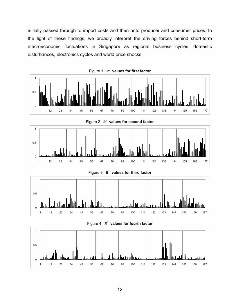
In attempting to assign interpretations to the factors, we are aware of the pitfalls
involved. The factor model suffers from a lack of identification because the estimated
factors are just linear combinations of the primitive shocks underlying business cycles.
Nevertheless, we follow Stock and Watson (2002b) and regress every variable in the
dataset against each factor to see if a particular factor is strongly related to a specific
group of macroeconomic variables. The 2R , or explanatory power, of the first four factors
for individual series are graphed as bar charts in Figures 1–4, where the numbers on the
horizontal axis refer to variables (see the appendix listing) and the vertical lines divide
them into the ten groupings of the previous section.
The first factor reflects the general business cycle in Singapore and places heavy
weights on regional economic series, domestic production, employment and exports. In
terms of sectoral breakdown, manufacturing, commerce and financial services are
strongly emphasized. This is very much in line with the regional hub status of Singapore
and her role as an exporter of high value-added parts and accessories in the electronics
supply chain based in Asia. By contrast, the second dynamic factor clearly picks out the
indicators associated with the local construction cycle and supporting services such as
real estate transactions and bank lending. Labour market variables and effective
exchange rates also load highly on this component.
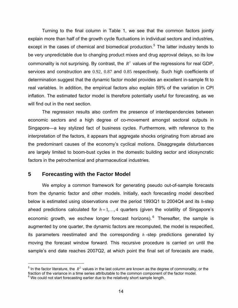
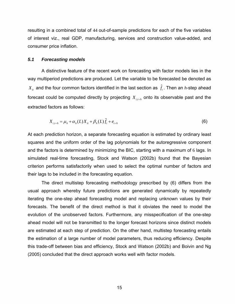
As we move to the other two factors, the heights of the bars in the graphs diminish
noticeably, testifying to their lower explanatory power. The third estimated factor seems to
be linked to the global tech cycle, the indigenous semiconductor industries and the
transportation sector. Domestic interest rates also figure prominently in this factor. The
fourth factor emphasizes nominal price series, especially the producer price index, trade
price indices, the oil price, and other world prices. Reflecting the openness of Singapore,
this factor primarily captures the external price shocks hitting the economy. As
Abeysinghe and Choy (2009) have shown, oil price hikes and foreign price increases are
2R4 These figures are derived from the trace statistic for the estimated factor model.
11
initially passed through to import costs and then onto producer and consumer prices. In
the light of these findings, we broadly interpret the driving forces behind short-term
macroeconomic fluctuations in Singapore as regional business cycles, domestic
disturbances, electronics cycles and world price shocks.
Figure 1 values for first factor 2R
0
0.5
1
1 12 23 34 45 56 67 78 89 100 111 122 133 144 155 166 177
Figure 2 values for second factor 2R
0
0.5
1
1 12 23 34 45 56 67 78 89 100 111 122 133 144 155 166 177
Figure 3 values for third factor 2R
0
0.5
1
1 12 23 34 45 56 67 78 89 100 111 122 133 144 155 166 177
Figure 4 values for fourth factor 2R
0
0.5
1
1 12 23 34 45 56 67 78 89 100 111 122 133 144 155 166 177
12
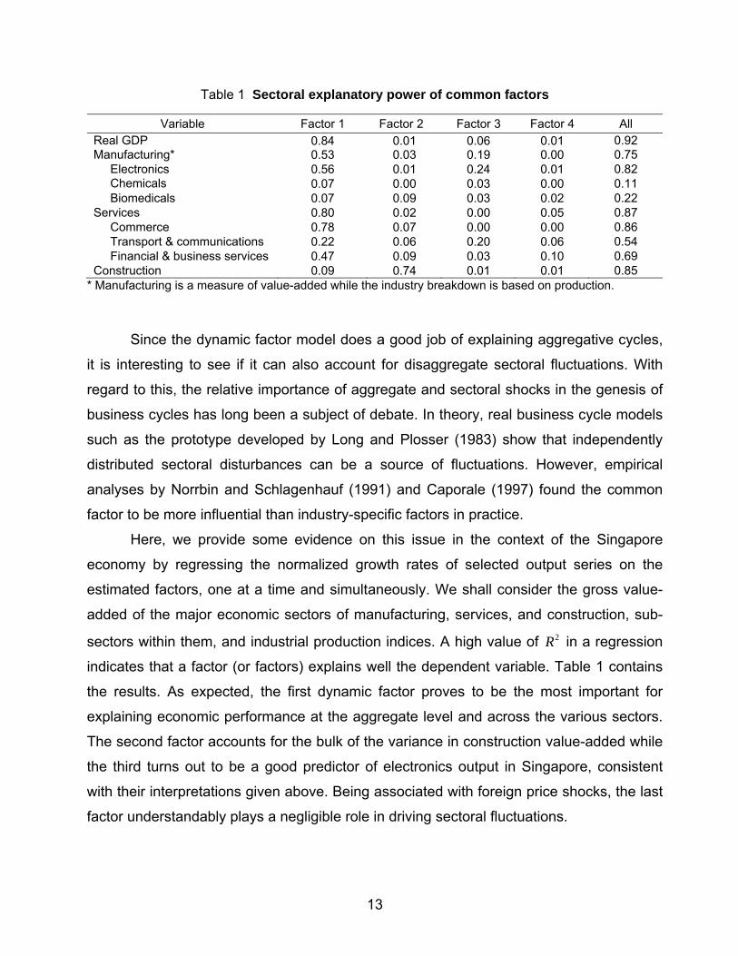
Table 1 Sectoral explanatory power of common factors
Variable Factor 1 Factor 2 Factor 3 Factor 4 All Real GDP 0.84 0.01 0.06 0.01 0.92 Manufacturing* 0.53 0.03 0.19 0.00 0.75 Electronics 0.56 0.01 0.24 0.01 0.82 Chemicals 0.07 0.00 0.03 0.00 0.11 Biomedicals 0.07 0.09 0.03 0.02 0.22 Services 0.80 0.02 0.00 0.05 0.87 Commerce 0.78 0.07 0.00 0.00 0.86 Transport & communications 0.22 0.06 0.20 0.06 0.54 Financial & business services 0.47 0.09 0.03 0.10 0.69 Construction 0.09 0.74 0.01 0.01 0.85
* Manufacturing is a measure of value-added while the industry breakdown is based on production.
Since the dynamic factor model does a good job of explaining aggregative cycles,
it is interesting to see if it can also account for disaggregate sectoral fluctuations. With
regard to this, the relative importance of aggregate and sectoral shocks in the genesis of
business cycles has long been a subject of debate. In theory, real business cycle models
such as the prototype developed by Long and Plosser (1983) show that independently
distributed sectoral disturbances can be a source of fluctuations. However, empirical
analyses by Norrbin and Schlagenhauf (1991) and Caporale (1997) found the common
factor to be more influential than industry-specific factors in practice.
Here, we provide some evidence on this issue in the context of the Singapore
economy by regressing the normalized growth rates of selected output series on the
estimated factors, one at a time and simultaneously. We shall consider the gross value-
added of the major economic sectors of manufacturing, services, and construction, sub-
sectors within them, and industrial production indices. A high value of 2R in a regression
indicates that a factor (or factors) explains well the dependent variable. Table 1 contains
the results. As expected, the first dynamic factor proves to be the most important for
explaining economic performance at the aggregate level and across the various sectors.
The second factor accounts for the bulk of the variance in construction value-added while
the third turns out to be a good predictor of electronics output in Singapore, consistent
with their interpretations given above. Being associated with foreign price shocks, the last
factor understandably plays a negligible role in driving sectoral fluctuations.
13
Turning to the final column in Table 1, we see that the common factors jointly
explain more than half of the growth cycle fluctuations in individual sectors and industries,
except in the cases of chemical and biomedical production.5 The latter industry tends to
be very unpredictable due to changing product mixes and drug approval delays, so its low
commonality is not surprising. By contrast, the 2R values of the regressions for real GDP,
services and construction are 0.92, 0.87 and 0.85 respectively. Such high coefficients of
determination suggest that the dynamic factor model provides an excellent in-sample fit to
real variables. In addition, the empirical factors also explain 59% of the variation in CPI
inflation. The estimated factor model is therefore potentially useful for forecasting, as we
will find out in the next section.
The regression results also confirm the presence of interdependencies between
economic sectors and a high degree of co-movement amongst sectoral outputs in
Singapore—a key stylized fact of business cycles. Furthermore, with reference to the
interpretation of the factors, it appears that aggregate shocks originating from abroad are
the predominant causes of the economy’s cyclical motions. Disaggregate disturbances
are largely limited to boom-bust cycles in the domestic building sector and idiosyncratic
factors in the petrochemical and pharmaceutical industries.
5 Forecasting with the Factor Model
We employ a common framework for generating pseudo out-of-sample forecasts
from the dynamic factor and other models. Initially, each forecasting model described
below is estimated using observations over the period 1993Q1 to 2004Q4 and its h-step
ahead predictions calculated for 1, , 4h = … quarters (given the volatility of Singapore’s
economic growth, we eschew longer forecast horizons). 6 Thereafter, the sample is
augmented by one quarter, the dynamic factors are recomputed, the model is respecified,
its parameters reestimated and the corresponding h -step predictions generated by
moving the forecast window forward. This recursive procedure is carried on until the
sample’s end date reaches 2007Q2, at which point the final set of forecasts are made,
2R5 In the factor literature, the values in the last column are known as the degree of commonality, or the
fraction of the variance in a time series attributable to the common component of the factor model. 6 We could not start forecasting earlier due to the relatively short sample length.
14
resulting in a combined total of 44 out-of-sample predictions for each of the five variables
of interest viz., real GDP, manufacturing, services and construction value-added, and
consumer price inflation.
5.1 Forecasting models
A distinctive feature of the recent work on forecasting with factor models lies in the
way multiperiod predictions are produced. Let the variable to be forecasted be denoted as
itX and the four common factors identified in the last section as t̂f . Then an h-step ahead
forecast could be computed directly by projecting ,i t hX + onto its observable past and the
extracted factors as follows:
,
ˆ( ) ( )i t h h h it h t t hX L X L f eμ α β+ = + + + + (6) At each prediction horizon, a separate forecasting equation is estimated by ordinary least
squares and the uniform order of the lag polynomials for the autoregressive component
and the factors is determined by minimizing the BIC, starting with a maximum of 6 lags. In
simulated real-time forecasting, Stock and Watson (2002b) found that the Bayesian
criterion performs satisfactorily when used to select the optimal number of factors and
their lags to be included in the forecasting equation.
The direct multistep forecasting methodology prescribed by (6) differs from the
usual approach whereby future predictions are generated dynamically by repeatedly
iterating the one-step ahead forecasting model and replacing unknown values by their
forecasts. The benefit of the direct method is that it obviates the need to model the
evolution of the unobserved factors. Furthermore, any misspecification of the one-step
ahead model will not be transmitted to the longer forecast horizons since distinct models
are estimated at each step of prediction. On the other hand, multistep forecasting entails
the estimation of a large number of model parameters, thus reducing efficiency. Despite
this trade-off between bias and efficiency, Stock and Watson (2002b) and Boivin and Ng
(2005) concluded that the direct approach works well with factor models.
15

On leaving the dynamic factors out of (6), we get univariate autoregressions for
each output and price variable. This constitutes the benchmark models with which the
performances of the factor forecasting models are compared. We pick the lag length of
the autoregressions through the BIC, with most of the AR models selected being of order
5 or 6, hence allowing complex roots to capture the cyclical behaviour of the data. Such
models are therefore not as naïve as they might seem to be. However, it should be noted
that the predictions from the AR models are generated iteratively rather than directly, as
this is what is usually done in practice.
The multivariate competitor to the foregoing models which we employ in the
forecast comparison is a vector autoregression that incorporates leading indicators. As
written out below, this model combines the rich dynamics of small-scale VARs with the
advantages of the leading indicator approach to forecasting:
1 1t t p t pY Y Y tτ η− −= + Γ + +Γ + (7)
where , [ ,t it tY X Z ′= ] tZ is a vector of macroeconomic and leading variables, iΓ are lag
coefficient matrices and tη is multivariate white noise. Again, the optimal lag length is
determined by the BIC, subject to 1 6p≤ ≤ . Once the VAR model has been estimated by
least squares, predictions at the various horizons are computed simply by iterating it h
steps forward.
The vector of stationary time series in (7) is always a subset of the full dataset
employed in the factor analysis, but it changes with the variable being forecasted. When
attempting to predict aggregate output growth, it is
[ , , , , ,t t t t t t ty GDP FGDP CLI ELI NEER CA ]′=
tNEER
tCA
, where is a weighted average of
incomes in Singapore’s major trading partners, CLI is the composite leading index,
is the electronics leading index, is the nominal effective exchange rate and
represents total construction contracts awarded—a leading series for the building industry.
For manufacturing and service sector growth, GDP is replaced by either manufacturing or
service value-added output and is dropped. A priori reasoning hints, and practical
tFORGDP
t
t
tELI
tCA
16
experimentation confirms, that foreign income and the leading indexes are not useful
predictors of Singapore’s construction sector. Consequently, the vector of
macroeconomic variables for forecasting the construction growth rate is
, the last entry representing the residential property price
index.
[ , ,t t ty CONSTR CA PPIRES ′=
[ , , ,t t t ty CPI GDP OIL WORLDC
]t
]t
In predicting price inflation, the endogenous vector is modified to
,tPI NEER ′= , in which the crude oil price and the foreign
price index serve as leading indicators of inflation. The variable is retained since
an effective exchange rate appreciation will mitigate imported sources of inflation while
GDP growth acts as a proxy for domestic inflationary pressures. This VAR model’s
predictive power will provide an instructive comparison with the dynamic factor model,
where the last included factor represents world price cycles.
tNEER
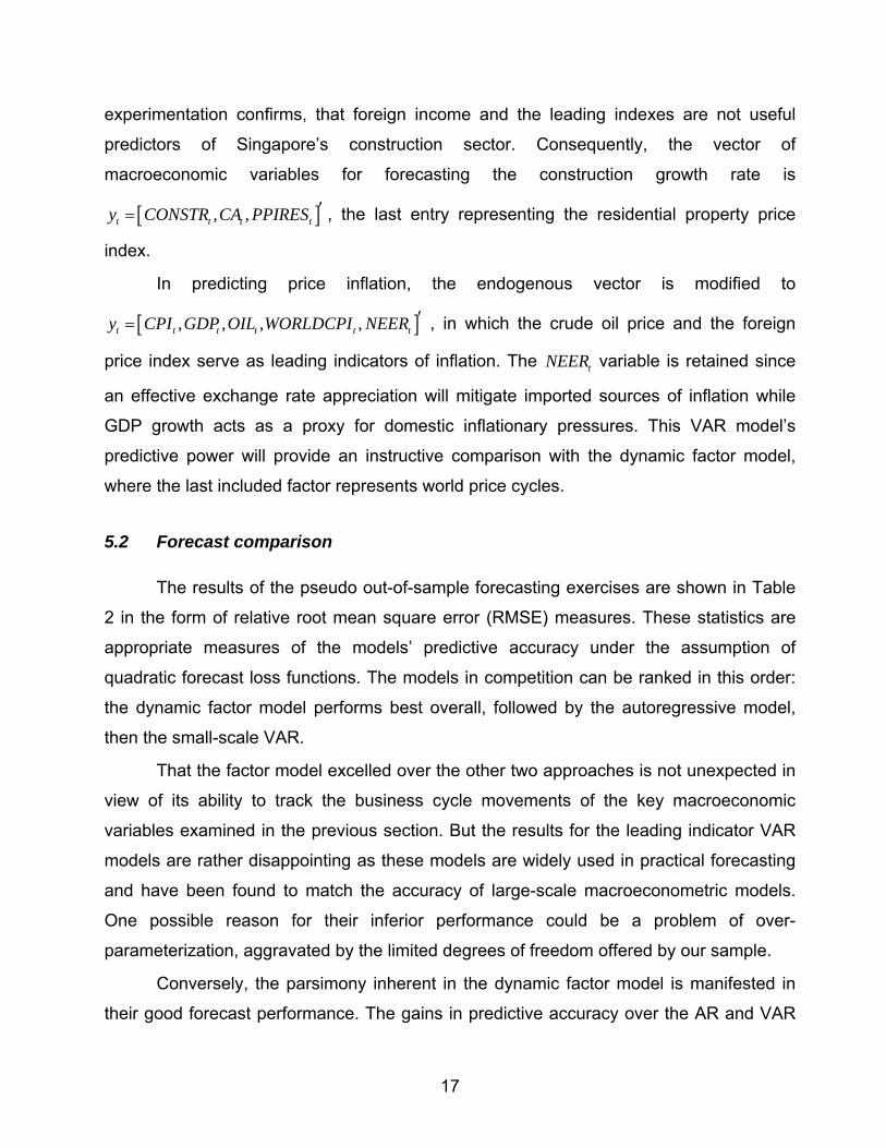
5.2 Forecast comparison
The results of the pseudo out-of-sample forecasting exercises are shown in Table
2 in the form of relative root mean square error (RMSE) measures. These statistics are
appropriate measures of the models’ predictive accuracy under the assumption of
quadratic forecast loss functions. The models in competition can be ranked in this order:
the dynamic factor model performs best overall, followed by the autoregressive model,
then the small-scale VAR.
That the factor model excelled over the other two approaches is not unexpected in
view of its ability to track the business cycle movements of the key macroeconomic
variables examined in the previous section. But the results for the leading indicator VAR
models are rather disappointing as these models are widely used in practical forecasting
and have been found to match the accuracy of large-scale macroeconometric models.
One possible reason for their inferior performance could be a problem of over-
parameterization, aggravated by the limited degrees of freedom offered by our sample.
Conversely, the parsimony inherent in the dynamic factor model is manifested in
their good forecast performance. The gains in predictive accuracy over the AR and VAR
17
models are apparent at the 1 to 3 quarters horizons for real GDP and services output
growth. In the cases of construction value-added and CPI inflation, the factor model
outperformed the other models at all prediction horizons, confirming that the cyclical
information summarized by the set of common factors is more comprehensive than that
found in individual macroeconomic variables. However, neither the factor nor the VAR
model could beat the benchmark autoregressive predictions in the case of manufacturing
growth. This finding has been pre-empted by the weaker explanatory power of the
empirical factors for the manufacturing sector and its constituent industries.
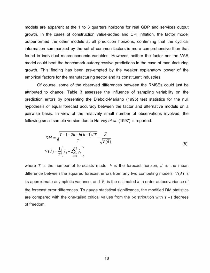
Of course, some of the observed differences between the RMSEs could just be
attributed to chance. Table 3 assesses the influence of sampling variability on the
prediction errors by presenting the Diebold-Mariano (1995) test statistics for the null
hypothesis of equal forecast accuracy between the factor and alternative models on a
pairwise basis. In view of the relatively small number of observations involved, the
following small sample version due to Harvey et al. (1997) is reported:
( )
1
01
1 2 1 /
( )
1 ˆ ˆ( ) 2h
kk
T h h h T dDMT V d
V dT
γ γ−
+
+ − + −= ⋅
⎛ ⎞= +⎜ ⎟
⎝ ⎠∑
(8)
where T is the number of forecasts made, h is the forecast horizon, d is the mean
difference between the squared forecast errors from any two competing models, ( )V d is
its approximate asymptotic variance, and ˆkγ is the estimated k-th order autocovariance of
the forecast error differences. To gauge statistical significance, the modified DM statistics
are compared with the one-tailed critical values from the t-distribution with degrees
of freedom.
1T −
18
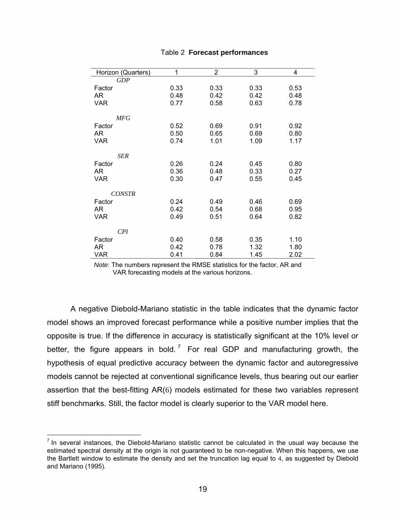
Table 2 Forecast performances
Horizon (Quarters) 1 2 3 4 GDP
Factor 0.33 0.33 0.33 0.53 AR 0.48 0.42 0.42 0.48 VAR 0.77 0.58 0.63 0.78
MFG
Factor 0.52 0.69 0.91 0.92 AR 0.50 0.65 0.69 0.80 VAR 0.74 1.01 1.09 1.17
SER
Factor 0.26 0.24 0.45 0.80 AR 0.36 0.48 0.33 0.27 VAR 0.30 0.47 0.55 0.45
CONSTR
Factor 0.24 0.49 0.46 0.69 AR 0.42 0.54 0.68 0.95 VAR 0.49 0.51 0.64 0.82
CPI
Factor 0.40 0.58 0.35 1.10 AR 0.42 0.78 1.32 1.80 VAR 0.41 0.84 1.45 2.02
Note: The numbers represent the RMSE statistics for the factor, AR and VAR forecasting models at the various horizons.
A negative Diebold-Mariano statistic in the table indicates that the dynamic factor
model shows an improved forecast performance while a positive number implies that the
opposite is true. If the difference in accuracy is statistically significant at the 10% level or
better, the figure appears in bold. 7 For real GDP and manufacturing growth, the
hypothesis of equal predictive accuracy between the dynamic factor and autoregressive
models cannot be rejected at conventional significance levels, thus bearing out our earlier
assertion that the best-fitting AR(6) models estimated for these two variables represent
stiff benchmarks. Still, the factor model is clearly superior to the VAR model here.
7 In several instances, the Diebold-Mariano statistic cannot be calculated in the usual way because the estimated spectral density at the origin is not guaranteed to be non-negative. When this happens, we use the Bartlett window to estimate the density and set the truncation lag equal to 4, as suggested by Diebold and Mariano (1995).
19
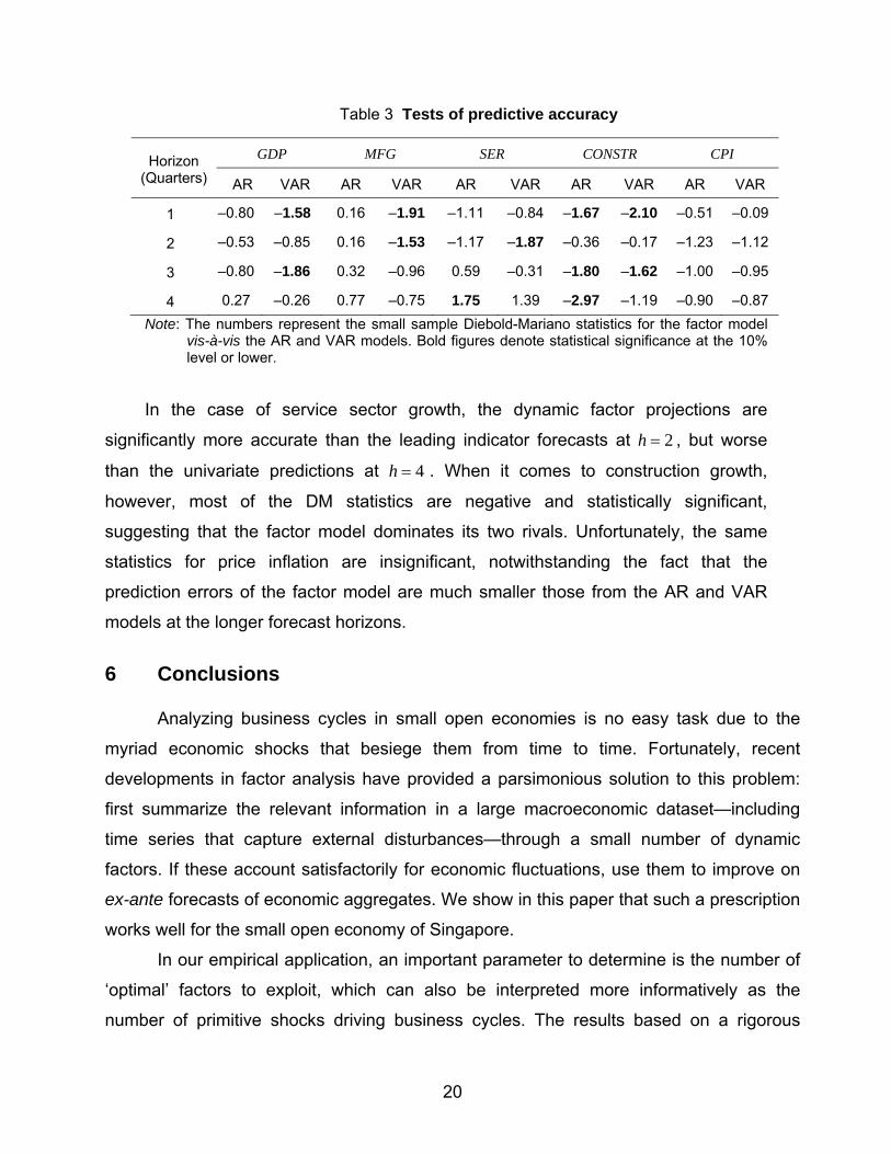
Table 3 Tests of predictive accuracy
Horizon (Quarters)
GDP MFG SER CONSTR CPI
AR VAR AR VAR AR VAR AR VAR AR VAR
1 –0.80 –1.58 0.16 –1.91 –1.11 –0.84 –1.67 –2.10 –0.51 –0.09
2 –0.53 –0.85 0.16 –1.53 –1.17 –1.87 –0.36 –0.17 –1.23 –1.12
3 –0.80 –1.86 0.32 –0.96 0.59 –0.31 –1.80 –1.62 –1.00 –0.95
4 0.27 –0.26 0.77 –0.75 1.75 1.39 –2.97 –1.19 –0.90 –0.87 Note: The numbers represent the small sample Diebold-Mariano statistics for the factor model
vis-à-vis the AR and VAR models. Bold figures denote statistical significance at the 10% level or lower.
In the case of service sector growth, the dynamic factor projections are
significantly more accurate than the leading indicator forecasts at , but worse
than the univariate predictions at
2h =
4h = . When it comes to construction growth,
however, most of the DM statistics are negative and statistically significant,
suggesting that the factor model dominates its two rivals. Unfortunately, the same
statistics for price inflation are insignificant, notwithstanding the fact that the
prediction errors of the factor model are much smaller those from the AR and VAR
models at the longer forecast horizons.
6 Conclusions
Analyzing business cycles in small open economies is no easy task due to the
myriad economic shocks that besiege them from time to time. Fortunately, recent
developments in factor analysis have provided a parsimonious solution to this problem:
first summarize the relevant information in a large macroeconomic dataset—including
time series that capture external disturbances—through a small number of dynamic
factors. If these account satisfactorily for economic fluctuations, use them to improve on
ex-ante forecasts of economic aggregates. We show in this paper that such a prescription
works well for the small open economy of Singapore.
In our empirical application, an important parameter to determine is the number of
‘optimal’ factors to exploit, which can also be interpreted more informatively as the
number of primitive shocks driving business cycles. The results based on a rigorous
20

procedure suggest that four dynamic factors are sufficient to explain over half of the
observed macroeconomic fluctuations in Singapore. This is a small number when viewed
in an international perspective—typically, five to six factors are needed to explain the
same proportion of variance in larger economies. Thus, Singapore’s business cycles
seem to be caused by a few relatively large shocks originating from the world at large, its
neighbours in Asia, the global demand for electronics, and the domestic construction
industry.
Regardless of the economic interpretations given to the dynamic factors, prediction
based on them can be carried out by using the estimated factors in conjunction with a
direct multistep forecasting approach. We find that the recursive forecasts of real activity
and price inflation in Singapore produced by the factor model are generally more accurate
than those from univariate autoregressions and leading indicator VAR models, even
though the differences in forecast performance are not always significant. In conclusion,
we might say that the dynamic factor model has proven to be a useful technique for
analyzing and forecasting the business cycles of small open economies.
21
Appendix: Data Listing
Series Mnemonic Source Transformation
Foreign real GDPs (12)
1. USA USAGDP ) ) 2. Japan JAPGDP ) ) 3. Korea KORGDP ) Econometric ) 4. Rest of the OECD ROECDGDP ) Studies ) 5. Malaysia MALGDP ) Unit, ) Growth 6. Indonesia INDOGDP ) National ) rates 7. Thailand THAIGDP ) University ) 8. Philippines PHILGDP ) of Singapore ) 9. Taiwan TAIGDP ) ) 10. Hong Kong HKGDP ) ) 11. China CHINGDP ) ) 12. Foreign GDP FORGDP ) )
Foreign leading indexes (6)
13. USA USACLI ) ) 14. Japan JAPCLI ) ) Deviations 15. Germany GERCLI ) SourceOECD ) from 16. UK UKCLI ) ) trend 17. 4 big European EUROCLI ) ) 18. 5 major Asian ASIACLI ) )
Foreign stock prices (10)
19. US USASPI ) ) 20. Japan JAPSPI ) ) 21. Germany GERSPI ) ) 22. UK UKSPI ) ) 23. Korea KORSPI ) Bloomberg ) Growth 24. Malaysia MALSPI ) ) rates 25. Indonesia INDOSPI ) ) 26. Thailand THAISPI ) ) 27. Philippines PHILSPI ) ) 28. Hong Kong HKSPI ) )
Foreign real interest rates (3)
29. US (3-mth LIBOR – CPI ∆) USAIR ) International ) 30. Japan (3-mth LIBOR – CPI ∆) JAPIR ) Financial ) Levels 31. UK (3-mth LIBOR – CPI % ∆) UKIR ) Statistics )
22
Series Mnemonic Source Transformation
World electronics (7)
32. Global semiconductor sales CHIP SIA Growth rates 33. US Tech Pulse Index TECH New York Fed Growth rates 34. Nasdaq index NASDAQ Bloomberg Growth rates 35. US new orders for electronics
(excl. semiconductors) USNO US Census Bureau Growth rates
36. US shipments-to-inventories ratio for electronics (excl. semiconductors)
USSI US Census Bureau Growth rates
37. Book-to-bill ratio BBR SEMI Levels 38. Electronics Leading Index ELI Authors Growth rates
World prices (3)
39. Real oil price (Dubai Fateh – World CPI ∆) OIL ) International ) Growth
40. Non-fuel commodity prices NONOIL ) Financial ) rates 41. World CPI WORLDCPI ) Statistics )
Real GDP components (7)
42. Real GDP GDP ) ) 43. Private consumption CON ) ) 44. Government consumption GCON ) ) Growth 45. Gross fixed capital formation GFCF ) STS ) rates 46. Transport equipment GFCFTPT ) ) 47. Machinery, equipment
& software GFCFMEQ ) )
48. Net exports NX ) ) Gross value-added (13)
49. Manufacturing MFG ) ) 50. Construction CONSTR ) ) 51. Services SER ) ) 52. Commerce COMM ) ) 53. Wholesale & retail trade WRTRADE ) ) 54. Hotels & restaurants* HOTREST ) STS ) Growth 55. Transport & Communications* TRANSCOM ) ) rates 56. Transport & storage* TRANSTOR ) ) 57. Information & communications INFOCOM ) ) 58. Financial & Business Services FINBIZ ) ) 59. Financial services FIN ) ) 60. Business services BIZ ) ) 61. Other Services OTHER ) )
23
Series Mnemonic Source Transformation
Industrial production (7)
62. Total IIP ) ) 63. Electronics IIPELEC ) ) 64. Chemicals IIPCHEM ) STS ) Growth 65. Biomedicals IIPBIO ) ) rates 66. Precision engineering IIPPRE ) ) 67. Transport engineering IIPTPT ) ) 68. General manufacturing IIPGEN ) )
Business surveys (17)
69. Mfg investment commitments COMMIT ) Growth rates 70. General expectations for mfg EXPMFG ) ) 71. Employment expectations for mfg EMPMFG ) ) 72. General expectations for services EXPSER ) ) 73. Wholesale & retail trade EXPWRTRADE ) ) 74. Hotels & catering EXPHOTREST ) ) 75. Transport & storage EXPTRANSTOR ) ) 76. Financial services EXPFIN ) ) Net 77. Business services EXPBIZ ) STS ) balances 78. Real estate EXPESTATE ) ) of 79. Employment expectations for
services EMPSER ) ) firms
80. Wholesale & retail trade EMPWRTRADE ) ) 81. Hotels & catering EMPHOTREST ) ) 82. Transport & storage EMPTRANSTOR ) ) 83. Financial services EMPFIN ) ) 84. Business services EMPBIZ ) ) 85. Real estate EMPESTATE ) )
Construction (14)
86. GFCF in construction & works GFCFCONSTR ) ) 87. Residential buildings GFCFRES ) ) 88. Non-residential buildings GFCFNRES ) ) 89. Others GFCFOTHER ) STS ) Growth 90. Contract awards CA ) ) rates 91. Public CAPUB ) ) 92. Private CAPTE ) ) 93. Residential buildings CARES ) ) 94. Commercial buildings CACOMM ) ) 95. Civil engineering & others CACIVIL ) )
24
Series Mnemonic Source Transformation
96. Property price index (residential) PPIRES ) STS ) Growth 97. Property price index (office) PPIOFF ) ) rates
98. Property price index (shop) PPISHOP ) ) 99. Resale price index RESALE ) ) Sectoral Indicators (16) 100. Retail sales volume RETAIL ) ) 101. Car registrations CAR ) ) 102. Visitor arrivals* VISIT ) ) 103. Air cargo handled AIR ) ) 104. Sea cargo handled SEA ) ) 105. Electricity generation ELECTRIC ) ) 106. Composite leading index CLI ) ) 107. Formation of companies FORM ) STS ) Growth 108. Manufacturing FORMMFG ) ) rates 109. Construction FORMCONSTR ) ) 110. Wholesale & retail trade FORMWRTRADE ) ) 111. Hotels & restaurants FORMHOTREST ) ) 112. Transport & storage FORMTRANSTOR ) ) 113. Information & comms FORMINFOCOM ) ) 114. Financial & insurance FORMFIN ) ) 115. Real estate & leasing FORMESTATE ) ) External Trade (16) 116. Exports of goods & services X ) ) 117. Imports of goods and services M ) ) 118. Exports of goods GX ) ) 119. Oil OGX ) ) 120. Non-oil NOGX ) ) 121. Imports of goods GM ) ) 122. Oil OGM ) STS ) Growth 123. Non-oil NOGM ) ) rates 124. Exports of services SX ) ) 125. Imports of services SM ) ) 126. Domestic exports DX ) ) 127. Oil ODX ) ) 128. Non-oil NODX ) ) 129. Re-exports RX ) ) 130. Oil* ORX ) ) 131. Non-oil NORX ) )
25
Series Mnemonic Source Transformation
Price Indices (14) 132. Export price index XPI ) ) 133. Oil OXPI ) ) 134. Non-oil NOXPI ) ) 135. Import price index MPI ) ) 136. Oil OMPI ) ) 137. Non-oil NOMPI ) ) 138. Terms of trade TOT ) STS ) Growth 139. Consumer price index CPI ) ) rates 140. Domestic supply price index DSPI ) ) 141. Manufactured price index SMPI ) ) 142. GDP deflator PGDP ) ) 143. Manufacturing deflator PMFG ) ) 144. Construction deflator PCONSTR ) ) 145. Services deflator PSER ) ) Labour Market (7) 146. Changes in employment EMP ) Levels 147. Retrenchments RETRENCH ) Growth rates 148. Unemployment rate (overall) U ) STS Levels 149. Unemployment rate (resident) URES ) Levels 150. Unit labour costs ULC ) Growth rates 151. Manufacturing unit labour costs MULC ) Growth rates 152. Manufacturing unit business costs MUBC ) Growth rates
Financial (17) 153. Stock prices SES ) Growth rates 154. 3-mth interbank rate INTER ) Levels 155. 1-yr treasury bill yield TB ) Levels 156. 2-yr bond yield BOND2 ) Levels 157. 5-yr bond yield BOND5 ) Levels 158. Prime lending rate PLR ) Levels 159. Nominal effective exchange rate NEER ) STS ) 160. Real effective exchange rate REER ) ) 161. Singapore dollar to US$ USD ) ) 162. Singapore dollar to Pound POUND ) ) Growth 163. Singapore dollar to Yen YEN ) ) rates 164. Singapore dollar to Malaysian $ RINGGIT ) ) 165. Singapore dollar to HK$ HKD ) )
26
Series Mnemonic Source Transformation
166. Singapore dollar to Korean won WON ) ) 167. Singapore dollar to Taiwan $ NTD ) STS ) Growth 168. Singapore dollar to Indo rupiah* RUPIAH ) ) rates 169. Singapore dollar to Thai baht BAHT ) ) Monetary (8) 170. M1 M1 ) ) 171. M3 M3 ) ) 172. Bank loans LOAN ) ) 173. Manufacturing LOANMFG ) STS ) Growth 174. Building & construction LOANCONSTR ) ) rates 175. Commerce LOANCOMM ) ) 176. Financial institutions LOANFIN ) ) 177. Professional & pte individuals LOANPRO ) )
Note: Figures in parentheses represent the number of variables in each category. STS refers to the Singapore Department of Statistics online time series database. Time series adjusted for outliers are marked with an asterisk.
27
References Abeysinghe, T, Choy KM. 2009. Inflation, exchange rate and the Singapore economy: a
policy simulation. In Singapore and Asia: Impacts of the Global Financial Tsunami and Other Economic Issues, Sng HY, Chia WM (eds.). World Scientific Publishing: Singapore.
Artis MJ, Banerjee A, Marcellino M. 2005. Factor forecasts for the UK. Journal of
Forecasting 24: 52–60. Bai J, Ng S. 2002. Determining the number of factors in approximate factor models.
Econometrica 70: 191–221. Bai J, Ng S. 2007. Determining the number of primitive shocks in factor models. Journal
of Business and Economic Statistics 25: 52–60. Boivin J, Ng S. 2005. Understanding and comparing factor-based forecasts. International
Journal of Central Banking 1: 117–151. Bernanke BS, Boivin J, Eliasz P. 2005. Measuring the effects of monetary policy: a factor-
augmented vector autoregressive (FAVAR) approach. The Quarterly Journal of Economics 120: 387–422.
Burns AM, Mitchell WC. 1946. Measuring Business Cycles. National Bureau of Economic
Research: New York. Caporale GM. 1997. Sectoral shocks and business cycles: a disaggregated analysis of
output fluctuations in the UK. Applied Economics 29: 1477–1482.
Chow HK. 1993. Performance of the official composite leading index in monitoring the Singapore economy. Asian Economic Journal 7: 25–34.
Chow HK, Choy KM. 1995. Economic leading indicators for tracking Singapore’s growth cycle. Asian Economic Journal 9: 177–191.
Chow HK, Choy KM. 2006. Forecasting the global electronics cycle with leading indicators: a Bayesian VAR approach. International Journal of Forecasting 22: 301–315.
Choy KM. 2009. Business cycles in Singapore: stylized facts for a small open economy. Pacific Economic Review, forthcoming.
Danthine JP, Girardin M. 1989. Business cycles in Switzerland: a comparative study. European Economic Review 33: 31–50.
28
Department of Statistics, Singapore. 2004. Singapore’s growth chronology, coincident and leading indicators. Information Paper on Economic Statistics.
Diebold FX, Mariano RS. 1995. Comparing predictive accuracy. Journal of Business and
Economic Statistics 13: 253–263. Englund P, Persson T, Svenson LEO. 1992. Swedish business cycles: 1861–1988.
Journal of Monetary Economics 30: 343–371. Forni M, Hallin M, Lippi M, Reichlin L. 2000. The generalized dynamic factor model:
identification and estimation The Review of Economics and Statistics 82: 540–554. Forni M, Hallin M, Lippi M, Reichlin L. 2003. Do financial variables help forecasting
inflation and real activity in the Euro area? Journal of Monetary Economics 50: 1243–1255.
García-Ferrer A, Poncela P. 2002. Forecasting European GNP data through common
factor models and other procedures. Journal of Forecasting 21: 225–244. Harvey D, Leybourne S, Newbold P. 1997. Testing the equality of prediction mean
squared errors. International Journal of Forecasting 13: 281–291. Kim K, Buckle RA, Hall VB. 1994. Key features of New Zealand business cycles. The
Economic Record 70: 56–72. Kim K, Choi YY. 1997. Business Cycles in Korea: is there any stylized feature? Journal of
Economic Studies 24: 275–293. Kose MA, Ostrok C, Whiteman CH. 2003. International business cycles: world, region,
and country-specific factors. American Economic Review 93: 1216–1239. Leung CF, Suen W. 2001. Some preliminary findings on Hong Kong business cycles.
Pacific Economic Review 6: 37−54. Long JB, Plosser CI. 1983. Real business cycles. Journal of Political Economy 91: 39−69. Norrbin SC. Schlagenhauf DE. 1991. The importance of sectoral and aggregate shocks in
business cycles. Economic Inquiry 29: 317−35. Quah D, Sargent TJ. 1993. A dynamic index model for large cross sections. In Business
Cycles, Indicators, and Forecasting, Stock JH, Watson MW (eds). University of Chicago Press: Chicago.
Sargent TJ, Sims CA. 1977. Business cycle modeling without pretending to have too
much a priori economic theory. In New Methods in Business Cycle Research, Sims CA (ed.). Federal Reserve Bank of Minneapolis: Minneapolis.
29
30
Schumacher C. 2007. Forecasting German GDP using alternative factor models based on large datasets. Journal of Forecasting 26: 271–302.
Stock JH, Watson MW. 1989. New indexes of coincident and leading economic indicators.
NBER Macroeconomics Annual. Stock JH, Watson MW. 2002a. Forecasting using principal components from a large
number of predictors. Journal of the American Statistical Association 97: 1167–1179.
Stock JH, Watson MW. 2002b. Macroeconomic forecasting using diffusion indexes.
Journal of Business and Economic Statistics 20: 147–162.