ANALYTICAL AND EXPERIMENTAL INVESTIGATIONS OF …smart.ippt.gov.pl/stec_graduates/stes_final_bochenski_marcin.pdf · 1 ANALYTICAL AND EXPERIMENTAL INVESTIGATIONS OF AN AUTOPARAMETRIC

1

ANALYTICAL AND EXPERIMENTAL INVESTIGATIONS OF AN

AUTOPARAMETRIC BEAM STRUCTURE

M. Bochenski*(1)

, J. Warminski*, M. P. Cartmell

†

* Lublin University of Technology, Poland

e-mail: [email protected], [email protected]

†University of Glasgow, UK

e-mail: [email protected]

Keywords: Autoparametric Vibrations, Hamilton Principle, Composite Beam

Abstract. This paper concerns theoretical and experimental investigations of vibrations

of an autoparametric system composed of two beams with rectangular cross sections and

essentially different flexibilities in two orthogonal directions. Differential equations of

motion and associated boundary conditions based on the Hamilton principle of least

action, are derived to third order approximation. Experimental tests of the system

response, under random and harmonic excitations for the 1:4 internal resonance

condition are performed, and then the most important vibration modes are extracted. It is

shown that certain modes in the stiff and flexible directions of both beams may interact,

and, intuitively unexpected out-of-plane motion may also appear.

1 INTRODUCTION

Beam structures are common in mechanical and civil engineering1,2

. Linear and nonlinear

models of a single beam are studied extensively in many papers. Large vibrations of non-

planar motion of inextensional beams are considered in3. Equation of motions with nonlinear

curvatures and nonlinear inertia terms are derived systematically to third order approximation,

taking into account bending about two principal axes and torsion of the beam. Reduction of

the model into two differential equations is carried out by expressing twisting of the beam

versus its bending in two directions. The response of such a nonlinear model when excited

harmonically by an external, distributed, force is presented in4. Paper

5 presents the influence

of parametric excitation on a single vertical beam response generated in a perpendicular plane

III ECCOMAS THEMATIC CONFERENCE ON SMART STRUCTURES AND MATERIALS

W. Ostachowicz, J. Holnicki-Szulc, C. Mota Soares et al. (Eds.)

Gdansk, Poland, July 9–11, 2007

M. Bochenski, J. Warminski, M. P. Cartmell

2

to that of the excitation. It is shown that a few resonances can be excited simultaneously and

that a weaker type of coupling can modify that of stronger coupling to a significant extent.

Non-planar motion of a metal cantilever beam exited by vertical harmonic motion of the

support is also presented in6. Bifurcation analysis shows different possible vibrations of the

beam and five branches of the dynamic solution. Periodic, quasi-periodic and chaotic motions

are found near the main parametric resonance. Because of a well separated torsional

frequency, the influence of torsional inertia is neglected in the model. A study of nonlinear

vibrations of metallic cantilever beams subjected to transverse harmonic excitations is given

in7. Experimental and theoretical results are presented. The transfer of energy between widely

spaced modes via modulation, both in the presence and absence of a one-to-one internal

resonance is shown. Reduced-order models using the Galerkin discretisation are also

developed to predict experimentally observed motions.

More complicated situation may appear when instead of a single beam, a set of coupled

beams is to be analysed. Due to internal coupling caused by nonlinear terms resulting from

nonlinear geometry and inertia, autoparametric vibrations may appear8. In such a case, one

subsystem becomes a source of excitation to the other, and under some conditions this causes

an increase of a vibration amplitude and, moreover an energy transfer between different

vibration modes may take place9. This kind of coupling appears in, so called, “L” shaped

beam structures. In-plane motion analysis of such coupled beams is presented in10

. Derivation

of the equations of motion and dynamical boundary condition are shown there for a structure

flexible in one plane and stiff in the orthogonal direction. Analytical solutions are found when

the strongest coupling takes place, i.e. in the neighbourhood of the principal parametric

resonance and for a 2:1 internal resonance. Primary resonance of the first and the second

mode, and prediction of the Hopf bifurcation, are determined analytically. Experimental tests

of nonlinear motion in a coupled beam structure with quadratic nonlinearities are discussed

in11

and12

. Periodic, quasi-periodic, and chaotic responses, predicted by theory have been

confirmed. It has been shown that under a 2:1 internal resonance a very small excitation can

lead to chaotic response of the structure.

Another type of “L” shaped metal beam structure is explored in13-18

. The difference

between this and the models just summarised is that the beams are coupled in such a way that

their stiffnesses are essentially different in two orthogonal directions (see Fig.1). The effect of

non-linear coupling between bending modes of vibration is investigated theoretically and

experimentally in13,14

. The non-linear forced vibration responses show jumps at entry and

exits frequencies. Small non-linear interactions have significant effect under the 2:1 internal

resonance condition. Four mode interaction exhibits large amplitudes of indirectly excited

modes and saturation of the directly excited mode. Planar and non-planar motions of the

vertical beam for two simultaneous internal resonance conditions are presented in15

. The

combination and internal resonances give complicated responses and intermodal energy

exchange effects for small changes in external and internal tuning. Differential equations of

motion have been derived taking into account bending of the horizontal beam, and bending/

torsion of the vertical beam. Paper16

shows that violent non-synchronous torsion and bending


3

vibrations occur as a result of the existence of quadratic non-linear coupling terms and

internal resonance effects caused by strong four-mode interactions.

In spite of extensive investigations of the “L” shaped beam structure, there are no

literature analyses, to the authors’ knowledge, that take interaction between torsion and

bending in both of the coupled beams into account. The development of the mathematical

modelling is particularly important if the structure is made of composite material.

Additional interactions can be observed because of a natural closeness of the torsional

and bending modes frequencies, which are usually well separated for metallic structures.

This paper gives an extension of the analysis of the coupled beam structure presented

in papers13-18

. The systematic derivation of the differential equations of motions and

associated boundary conditions to third order approximation are given in the first part.

Then, the results of preliminary experimental tests are presented which show the modal

interactions and their influence on the structure’s response phenomena.

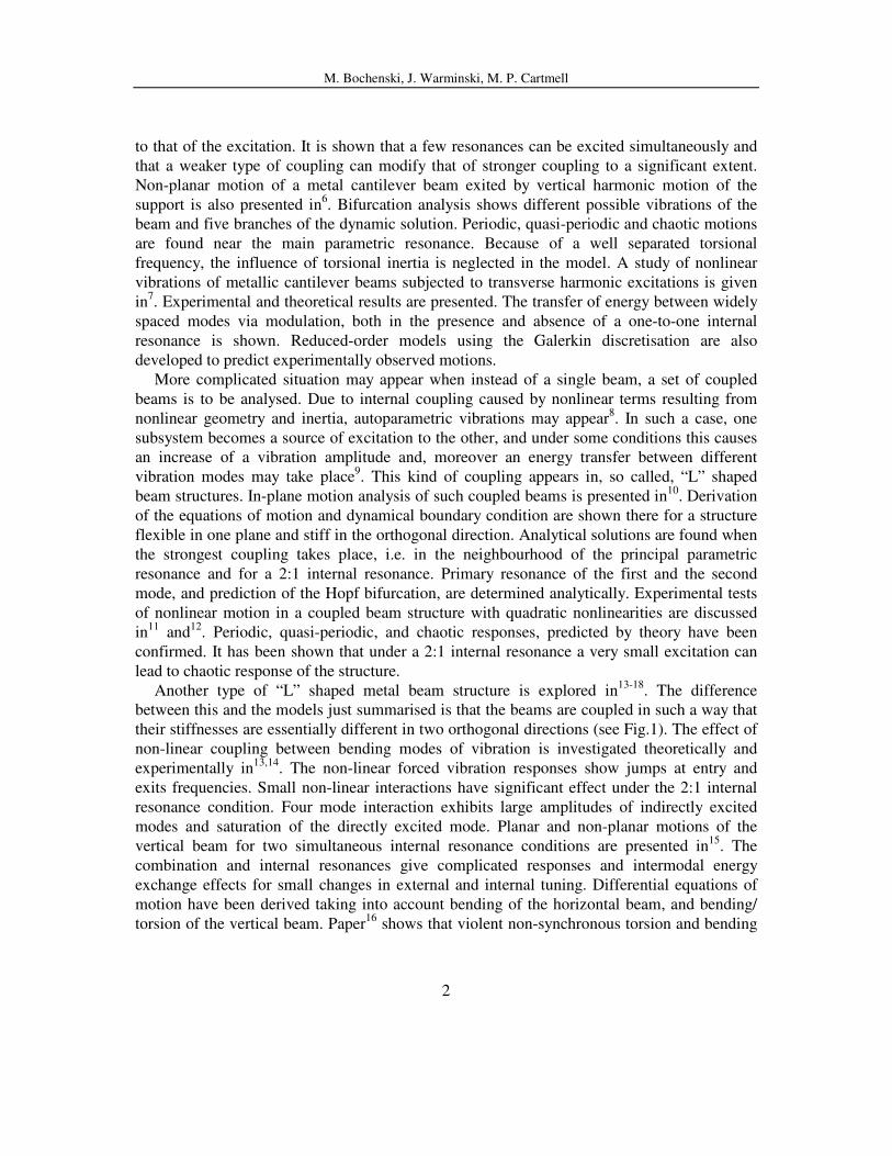
2 MODEL OF THE STRUCTURE

The structure considered in this paper consists of two thin beams made of glass-epoxy

composite with fibres oriented as follows: 0/90/45/-45/45/90/0 (Fig.1). Both beams are of

rectangular cross-section and are fixed in such a way that their flexibilities are essentially

different in the horizontal and vertical directions18

. They are clamped together at point C,

while the horizontal (primary) beam is fixed at the support B and can be excited by the shaker

in the Y1 direction. A lumped mass A attached at the top of the vertical (secondary) beam

allows for tuning of the structure for the required dynamical conditions.

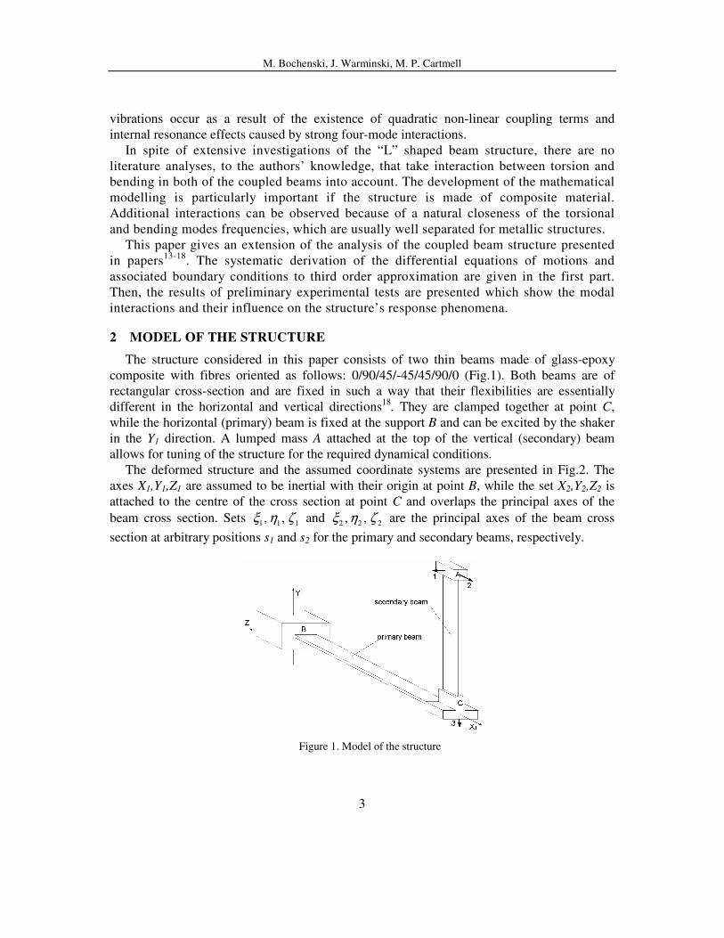
The deformed structure and the assumed coordinate systems are presented in Fig.2. The

axes X1,Y1,Z1 are assumed to be inertial with their origin at point B, while the set X2,Y2,Z2 is

attached to the centre of the cross section at point C and overlaps the principal axes of the

beam cross section. Sets 1 1 1, ,ξ η ζ and

2 2 2, ,ξ η ζ are the principal axes of the beam cross

section at arbitrary positions s1 and s2 for the primary and secondary beams, respectively.

Figure 1. Model of the structure


4

Figure 2. Deflected beam structure

The components 1 1( , )u s t ,

1 1( , )v s t , 1 1( , )w s t and

2 2( , )u s t , 2 2( , )v s t ,

2 2( , )w s t denote the

elastic displacement of the cross-section centroids of the primary and secondary beams (points

O1 and O2), while 1 1( , )s tφ , ( )1 1 ,s tψ , ( )1 1 ,s tθ and 2 2( , )s tφ , ( )2 2 ,s tψ , ( )2 2 ,s tθ represent the

rotations expressed by Euler angles.

3 EQUATIONS OF MOTION

The equations of free vibration of the structure given in Fig.1 are derived by applying

Hamilton’s principle of least action,

( )2

1

1 1 1 2 2 2 0

t

C C A A

t

T V F T V F T V T V dtδ − + + − + + − + − =∫ (1)

where 1T ,

1V , 1F ,

2T , 2V ,

2F denote the kinetic and potential energies and the constraint

equations of the primary and the secondary beams, and CT ,

CV , AT ,

AV , the kinetic and

potential energies of the masses C and A, respectively.

By introducing the notation 1

1 1 1 1 1

0

l

T V F h ds− + = ∫ , 2

2 2 2 2 2

0

l

T V F h ds− + = ∫ equation (1) can

then rewritten in the form,

2 1 2

1

1 1 2 2

0 0

0

t l l

c c A A

t

h ds h ds T V T V dtδ δ

+ + − + − = ∫ ∫ ∫ (2)

The kinetic energy of the primary beam results from translational and rotational motions of

the element shown in Fig.2a

a) b)


5

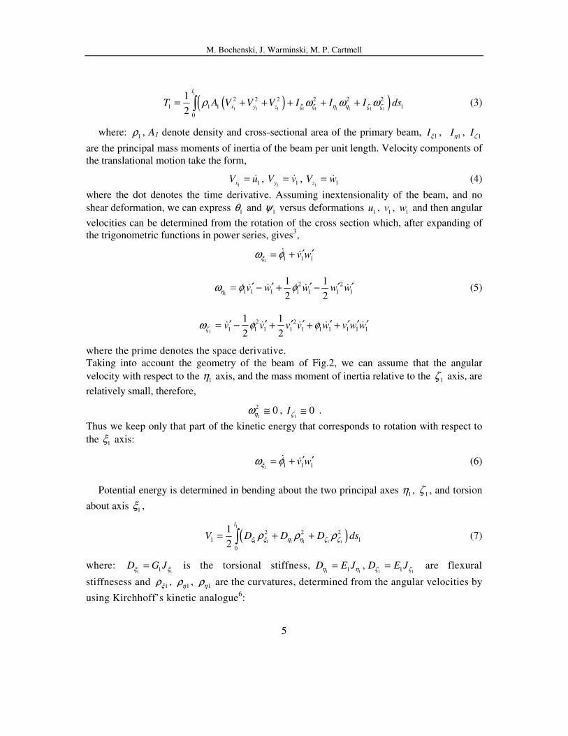
( )( )1

1 1 1 1 1 1 1 1 1

2 2 2 2 2 2

1 1 1 1

0

1

2

l

x y zT A V V V I I I dsξ ξ η η ζ ζρ ω ω ω= + + + + +∫ (3)

where: 1ρ , A1 denote density and cross-sectional area of the primary beam,

1Iξ , 1Iη ,

1Iζ

are the principal mass moments of inertia of the beam per unit length. Velocity components of

the translational motion take the form,

1 1xV u= & ,

1 1yV v= & , 1 1zV w= & (4)

where the dot denotes the time derivative. Assuming inextensionality of the beam, and no

shear deformation, we can express 1θ and

1ψ versus deformations 1u ,

1v , 1w and then angular

velocities can be determined from the rotation of the cross section which, after expanding of

the trigonometric functions in power series, gives3,

1 1 1 1v wξω φ ′ ′= +& &

1

2 2

1 1 1 1 1 1 1

1 1

2 2v w w w wηω φ φ′ ′ ′ ′ ′= − + −& & & & (5)

1

2 2

1 1 1 1 1 1 1 1 1 1

1 1

2 2v v v v w v w wζω φ φ′ ′ ′ ′ ′ ′ ′ ′= − + + +& & & & &

where the prime denotes the space derivative.

Taking into account the geometry of the beam of Fig.2, we can assume that the angular

velocity with respect to the 1η axis, and the mass moment of inertia relative to the

1ζ axis, are

relatively small, therefore,

1

2 0ηω ≅ , 1

0Iζ ≅ .

Thus we keep only that part of the kinetic energy that corresponds to rotation with respect to

the 1ξ axis:

1 1 1 1v wξω φ ′ ′= +& & (6)

Potential energy is determined in bending about the two principal axes 1η , 1ζ , and torsion

about axis 1ξ ,

( )1

1 1 1 1 1 1

2 2 2

1 1

0

1

2

l

V D D D dsξ ξ η η ζ ζρ ρ ρ= + +∫ (7)

where: 1 11D G Jξ ξ= is the torsional stiffness,

1 1 1 11 1,D E J D E Jη η ζ ζ= = are flexural

stiffnesess and 1ξρ ,

1ηρ , 1ηρ are the curvatures, determined from the angular velocities by

using Kirchhoff’s kinetic analogue6:


6

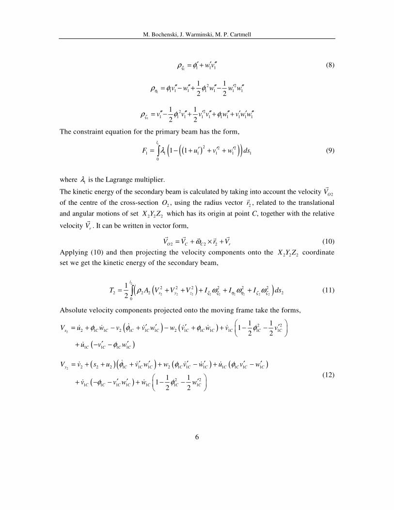
1 1 1 1w vξρ φ′ ′ ′′= + (8)

1

2 2

1 1 1 1 1 1 1

1 1

2 2v w w w wηρ φ φ′′ ′′ ′′ ′ ′′= − + −

1

2 2

1 1 1 1 1 1 1 1 1 1

1 1

2 2v v v v w v w wζρ φ φ′′ ′′ ′ ′′ ′′ ′ ′ ′′= − + + +

The constraint equation for the primary beam has the form,

( )( )( )1

2 2 2

1 1 1 1 1 1

0

1 1

l

F u v w dsλ ′ ′ ′= − + + +∫ (9)

where 1λ is the Lagrange multiplier.

The kinetic energy of the secondary beam is calculated by taking into account the velocity 2OVr

of the centre of the cross-section 2O , using the radius vector 2rr

, related to the translational

and angular motions of set 2 2 2X Y Z which has its origin at point C, together with the relative

velocity rVr

. It can be written in vector form,

2 2 2O C C rV V r Vω= + × +r r rr r

(10)

Applying (10) and then projecting the velocity components onto the 2 2 2X Y Z coordinate

set we get the kinetic energy of the secondary beam,

( )( )2

2 2 2 2 2 2 2 2 2

2 2 2 2 2 2

2 2 2 2

0

1

2

l

x y zT A V V V I I I dsξ ξ η η ζ ζρ ω ω ω= + + + + +∫ (11)

Absolute velocity components projected onto the moving frame take the forms,

( ) ( )

( )

2

2 2

2 1 1 2 1 1 1 2 1 1 1 1 1 1

1 1 1 1

1 11

2 2x C C C C C C C C C C C

C C C C

V u w v v w w v w v v

u v w

φ φ φ φ

φ

′ ′ ′ ′= + − + − + + − −

′ ′+ − −

&& & & & & &

&

( )( ) ( ) ( )

( )

2 2 2 2 1 1 1 2 1 1 1 1 1 1 1

2 2

1 1 1 1 1 1 1

1 11

2 2

y C C C C C C C C C C

C C C C C C C

V v s u v w w v w u v w

v v w w w

φ φ φ

φ φ

′ ′ ′ ′ ′ ′= + + + + − + −

′ ′ ′+ − − + − −

&& & & & &

& &

(12)


7

( )( )

( )

2

2 2

2 2 2 1 1 1 2 1 1 1 1 1 1 1

2 2

2 1 1 1 1 1 1 1 1 1 1

1 1

2 2

1 11

2 2

z C C C C C C C C C C

C C C C C C C C C C

V w s u v w s v v v w v w

v v w v v w w u v w

φ φ

φ

′ ′ ′ ′ ′ ′ ′ ′= − + + + − −

′ ′ ′ ′ ′ ′+ − + + + − −

& & & & & &

& & & & &

And, making assumptions similar to those of the primary beam,

2 2

2 0 0Iη ζω ≅ ≅

we get,

2 2 2 2v wξω φ ′ ′= +& & (13)

The potential energy of the secondary beam is expressed in the second local coordinate set,

denoted by index 2, and has an equivalent form to that of the primary beam,

( )2

2 2 2 2 2 2

2 2 2

2 2

0

1

2

l

V D D D dsξ ξ η η ζ ζρ ρ ρ= + +∫ (14)

with torsional and flexural stiffnesses,

2 2 2 2 2 22 2 2, ,D G J D E J D E Jξ ξ η η ζ ζ= = =

and curvatures,

2

2

2

2 2 2

2 2

2 2 2 2 2 2 2

2 2

2 2 2 2 2 2 2 2 2 2

1 1

2 2

1 1

2 2

w v

v w w w w

v v v v w v w w

ξ

η

ζ

ρ φ

ρ φ φ

ρ φ φ

′ ′ ′′= +

′′ ′′ ′′ ′ ′′= − + −

′′ ′′ ′ ′′ ′′ ′ ′ ′′= − + + +

(15)

The constraint equation for the secondary beam is defined as,

( )( )( )2

2 2 2

2 2 2 2 2 2

0

1 1

l

F u v w dsλ ′ ′ ′= − + + +∫ (16)

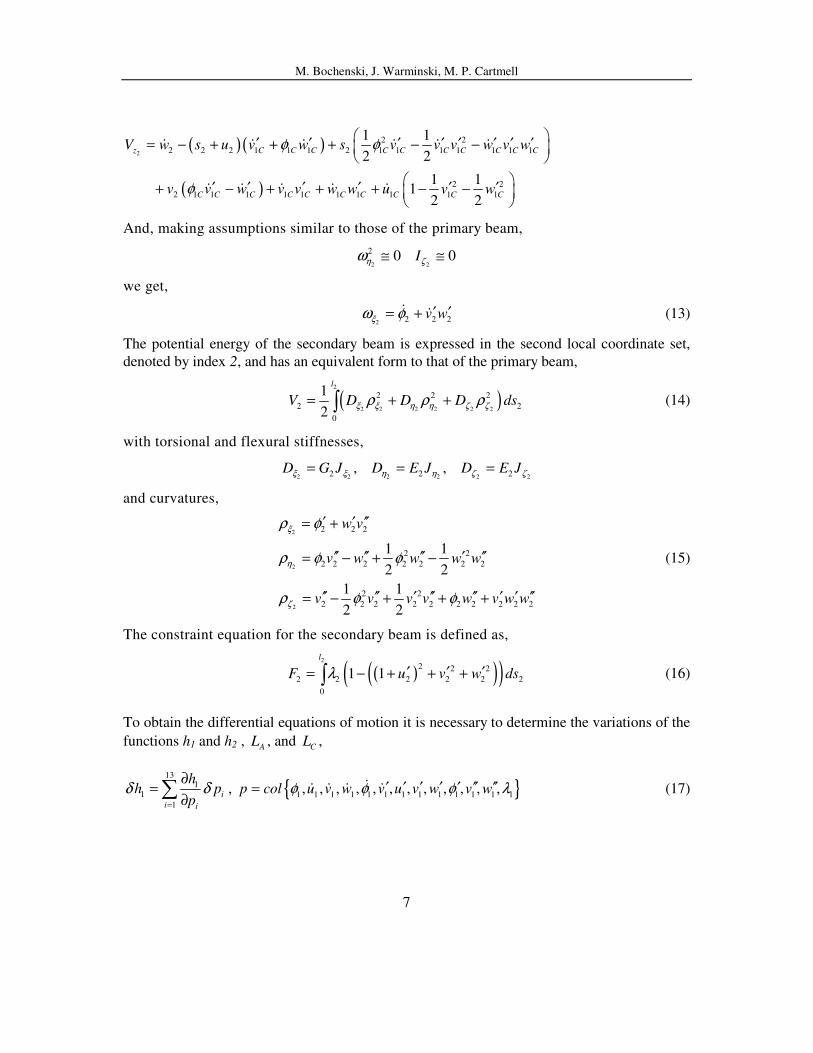
To obtain the differential equations of motion it is necessary to determine the variations of the

functions h1 and h2 , AL , and CL ,

131

1

1

i

i i

hh p

pδ δ

=

∂=

∂∑ , { }1 1 1 1 1 1 1 1 1 1 1 1 1

, , , , , , , , , , , ,p col u v w v u v w v wφ φ φ λ′ ′ ′ ′ ′ ′′ ′′= && & & & (17)


8

252

2

1

i

i i

hh q

qδ δ

=

∂=

∂∑ ,

{}

2, 2 2 2 2 2 2 2 2 2 2 2 2 2 1

2 1 1 1 1 1 1 1 1 1

, , , , , , , , , , , , , ,

, , , , , , , , ,C C C C C C C C C

q col u v w u v w v u v w v w

u v w v w v w

φ φ φ

λ φ φ

′ ′ ′ ′ ′ ′′ ′′=

′ ′ ′ ′

&& & & &

&& & & & &

(18)

10

1

C

C Ci

i Ci

LL p

pδ δ

=

∂=

∂∑ , { }1 1 1 1 1 1 1 1 1 1

, , , , , , , , ,C

p col v u v w v w v wφ φ ′ ′ ′ ′= && & & & & (19)

21

1

A

A Ai

i Ai

LL q

qδ δ

=

∂=

∂∑ ,

{

}2 2 2 2 2 2 2 2 2 2 2

2 1 1 1 1 1 1 1 1 1

, , , , , , , , , , ,

, , , , , , , , ,

A

C C C C C C C C C

q col u v w u v w v w v

w u v w v w v w

φ φ

φ φ

′ ′ ′=

′ ′ ′ ′ ′

&& & & & &

&& & & & & (20)

Integrating the variations by parts with respect to time between limits t1 and t2, and

remembering that variations at the time instances t1 and t2 are equal to zero we get,

2 1

1

2 2 2 3 2 3

1 1 1 1 1 1

1 12

1 1 1 1 1 1 1 1 1 10

2 2 3 2 2

1 1 1 1 1 1

1 12

1 1 1 1 1 11 1 1

t l

t

h h h h h hu v

u t u s v t v s t v s v s

h h h h h h hw

w t w s sw s t

δ δ

δ δφφ φφ

∂ ∂ ∂ ∂ ∂ ∂− − + − + − +

′ ′ ′ ′′∂ ∂ ∂ ∂ ∂ ∂ ∂ ∂ ∂ ∂ ∂ ∂ ∂

∂ ∂ ∂ ∂ ∂ ∂ ∂+ − − + + − − +

′ ′′′∂ ∂ ∂ ∂ ∂ ∂ ∂∂ ∂ ∂ ∂

∫ ∫& & &

&&

2

1

1 1

1

2 2 2 3 2 3

2 2 2 2 2 2 2 2

2 22

2 2 2 2 2 2 2 2 2 2 2 20

2 2 3 2

2 2 2 2 2 2

22

2 2 2 2 22 2 2

l

ds

h h h h h h h hu v

u u t u s v v t v s t v s v s

h h h h h hw

w w t w s w s t

δλλ

δ δ

δφ φ

∂

∂ ∂ ∂ ∂ ∂ ∂ ∂ ∂+ − − + − + − +

′ ′ ′ ′′∂ ∂ ∂ ∂ ∂ ∂ ∂ ∂ ∂ ∂ ∂ ∂ ∂ ∂ ∂

∂ ∂ ∂ ∂ ∂ ∂+ − − + + − −

′ ′′∂ ∂ ∂ ∂ ∂ ∂∂ ∂ ∂ ∂

∫& & &

&&

2

2 2

2 2 2

2 2 2

0h h

ds dts

δφ δλφ λ

∂ ∂ + =

′∂ ∂ ∂ (21)

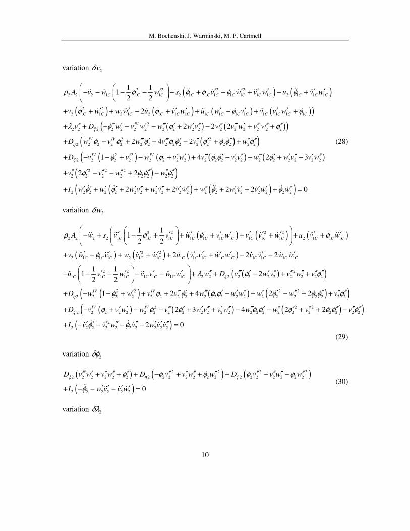
Next integrating by parts with respect to the space coordinates s1 and s2, and then collecting

terms for proper variations up to the third order, we get successive differential equations of

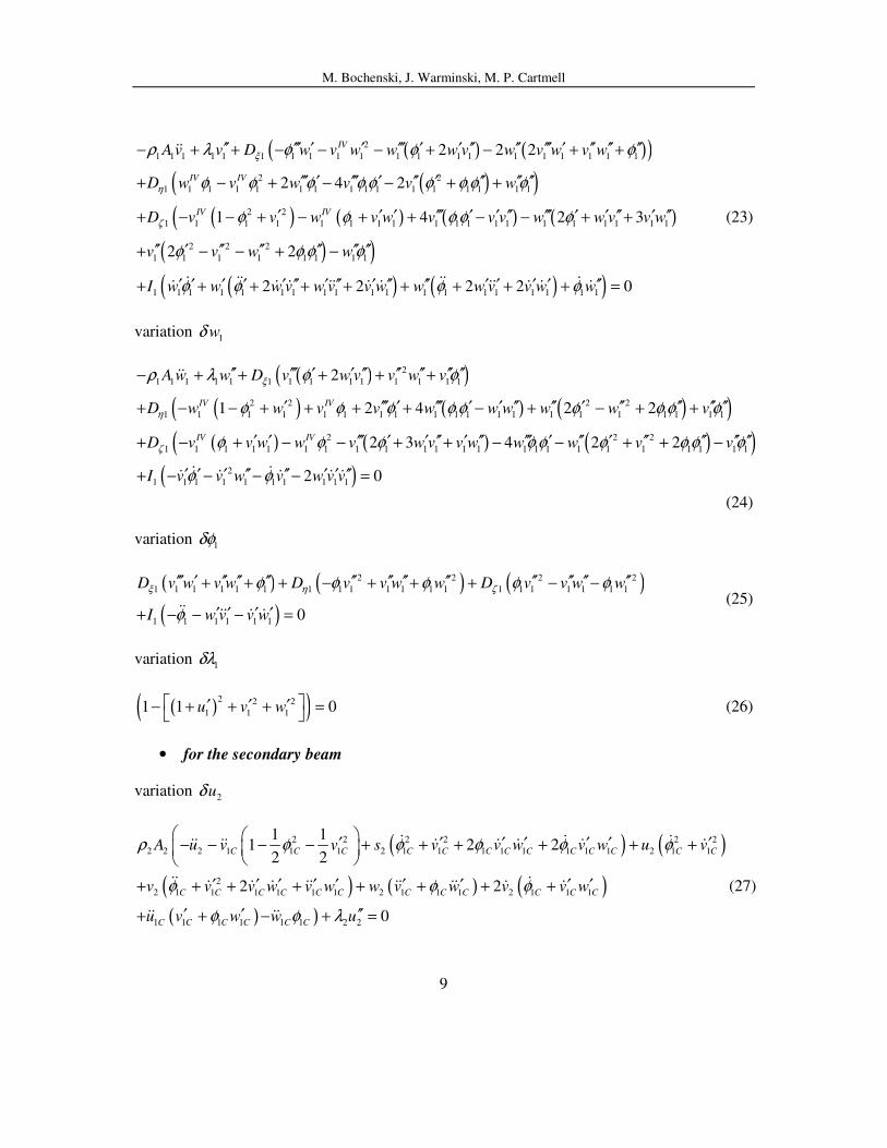
motions:

• for the primary beam

variation 1uδ

1 1 1 1 1 0A u uρ λ ′′− + =&& (22)

variation 1vδ


9

( ) ( )( )

( )( )( ) ( )

2

1 1 1 1 1 1 1 1 1 1 1 1 1 1 1 1 1 1 1 1

2 2

1 1 1 1 1 1 1 1 1 1 1 1 1 1 1 1

2 2

1 1 1 1 1 1 1 1 1 1 1 1

2 2 2

2 4 2

1 4

IV

IV IV

IV IV

A v v D w v w w w v w v w v w

D w v w v v w

D v v w v w v v

ξ

η

ζ

ρ λ φ φ φ

φ φ φ φ φ φ φ φ φ

φ φ φ φ

′′ ′′′ ′ ′ ′′′ ′ ′ ′′ ′′ ′′′ ′ ′′ ′′ ′′− + + − − − + − + +

′′′ ′ ′′′ ′ ′′ ′ ′′ ′′ ′′+ − + − − + +

′ ′ ′ ′′′ ′ ′+ − − + − + + −

&&

( ) ( )(( ) )

( ) ( )( )

1 1 1 1 1 1 1

2 2 2

1 1 1 1 1 1 1 1

1 1 1 1 1 1 1 1 1 1 1 1 1 1 1 1 1 1 1

2 3

2 2

2 2 2 2 0

v w w v v w

v v w w

I w w w v w v v w w w v v w w

φ

φ φ φ φ

φ φ φ φ

′′ ′′′ ′ ′ ′′ ′ ′′− + +

′′ ′ ′′ ′′ ′′ ′′ ′′+ − − + −

′ ′ ′ ′ ′ ′′ ′ ′′ ′ ′′ ′′ ′ ′ ′ ′ ′′+ + + + + + + + + =& && && && & & && & & && & & &

(23)

variation 1wδ

( )( )

( ) ( ) ( )( )( ) ( )

2

1 1 1 1 1 1 1 1 1 1 1 1 1 1

2 2 2 2

1 1 1 1 1 1 1 1 1 1 1 1 1 1 1 1 1 1 1 1

2

1 1 1 1 1 1 1 1 1 1 1 1 1

2

1 2 4 2 2

2 3 4

IV IV

IV IV

A w w D v w v v w v

D w w v v w w w w w v

D v v w w v w v v w

ξ

η

ζ

ρ λ φ φ


φ φ φ

′′ ′′′ ′ ′ ′′ ′′ ′′ ′′ ′′− + + + + +

′ ′′′ ′ ′′′ ′ ′ ′′ ′′ ′ ′′ ′′ ′′ ′′+ − − + + + + − + − + +

′ ′ ′′′ ′ ′ ′′ ′ ′′+ − + − − + + −

&&

( )( )( )

2 2

1 1 1 1 1 1 1 1 1 1

2

1 1 1 1 1 1 1 1 1 1

2 2

2 0

w w v v

I v v w v w v v

φ φ φ φ φ φ

φ φ

′′′ ′ ′′ ′ ′′ ′′ ′′ ′′− + + −

′ ′ ′ ′′ ′′ ′ ′ ′′+ − − − − =& && & & & &

(24)

variation 1δφ

( ) ( ) ( )

( )

2 2 2 2

1 1 1 1 1 1 1 1 1 1 1 1 1 1 1 1 1 1 1 1

1 1 1 1 1 10

D v w v w D v v w w D v v w w

I w v v w

ξ η ζφ φ φ φ φ

φ

′′′ ′ ′′ ′′ ′′ ′′ ′′ ′′ ′′ ′′ ′′ ′′ ′′+ + + − + + + − −

′ ′ ′ ′+ − − − =&& && & &

(25)

variation 1δλ

( )( )2 2 2

1 1 11 1 0u v w ′ ′ ′− + + + =

(26)

• for the secondary beam

variation 2uδ

( ) ( )

( ) ( ) ( )( )

2 2 2 2 2 2

2 2 2 1 1 1 2 1 1 1 1 1 1 1 1 2 1 1

2

2 1 1 1 1 1 1 2 1 1 1 2 1 1 1

1 1 1 1 1

1 11 2 2

2 2

2 2

C C C C C C C C C C C C C

C C C C C C C C C C C C

C C C C C

A u v v s v v w v w u v

v v v w v w w v w v v w

u v w w

ρ φ φ φ φ φ

φ φ φ

φ

′ ′ ′ ′ ′ ′ ′− − − − + + + + + +

′ ′ ′ ′ ′ ′ ′ ′ ′+ + + + + + + +

′ ′+ + −

& & &&& && & & & & &

&& && & & && && && & &

&& && )1 2 2 0C uφ λ ′′+ =

(27)


10

variation 2vδ

( ) ( )

( ) ( ) ( ) ( ))

2 2 2 2

2 2 2 1 1 1 2 1 1 1 1 1 1 1 2 1 1 1

2 2

2 1 1 2 1 2 1 1 1 1 1 1 1 1 1 1 1

2 2 2 2 2 2

1 11

2 2

2


C C C C C C C C C C C C C C

A v w w s v w v w u v w

v w w w u v w u w v v v w

v D w vξ

ρ φ φ φ φ φ

φ φ φ φ

λ φ

′ ′ ′ ′ ′ ′ ′− − − − − + − + − +

′ ′ ′ ′ ′ ′ ′ ′+ + + − + + − + +

′′ ′′′ ′+ + − −

&& &&&& && & & && &&

& && && & & && &&

( ) ( )( )

( )( )( ) ( ) ( ) ( )(

2

2 2 2 2 2 2 2 2 2 2 2

2 2

2 2 2 2 2 2 2 2 2 2 2 2 2 2 2 2

2 2

2 2 2 2 2 2 2 2 2 2 2 2 2 2 2 2 2 2 2

2 2 2

2 4 2

1 4 2 3

IV

IV IV

IV IV

w w w v w v w v w

D w v w v v w

D v v w v w v v v w w v v w

η

ζ

φ φ


φ φ φ φ φ

′ ′′′ ′ ′ ′′ ′′ ′′′ ′ ′′ ′′ ′′− + − + +

′′′ ′ ′′′ ′ ′′ ′ ′′ ′′ ′′+ − + − − + +

′ ′ ′ ′′′ ′ ′ ′′ ′′′ ′ ′ ′′ ′ ′′+ − − + − + + − − + +

+ ( ) )( ) ( )( )

2 2 2

2 2 2 2 2 2 2 2

2 2 2 2 2 2 2 2 2 2 2 2 2 2 2 2 2 2 2

2 2

2 2 2 2 0

v v w w

I w w w v w v v w w w v v w w

φ φ φ φ

φ φ φ φ

′′ ′ ′′ ′′ ′′ ′′ ′′− − + −

′ ′ ′ ′ ′ ′′ ′ ′′ ′ ′′ ′′ ′ ′ ′ ′ ′′+ + + + + + + + + =& && && && & & && & & && & & &

(28)

variation 2wδ

( ) ( ) ( )

( ) ( ) ( )

2 2 2 2

2 2 2 2 1 1 1 1 1 1 1 1 1 1 2 1 1 1

2 2

2 1 1 1 2 1 1 1 1 1 1 1 1 1 1 1

1 1

1 11

2 2

2 2 2

11

2


C C C C C C C C C C C C C C

C

A w s v v w v w v v w u v w

v w v w v w u v v w w v v w w

u v

ρ φ φ φ

φ

′ ′ ′ ′ ′ ′ ′ ′ ′ ′− + − + + + + + + +

′ ′ ′ ′ ′ ′ ′ ′ ′ ′+ − + + + + − −

′− −

&& && && & & && &&

&& && & & & & & & & & &

&& ( )( )

( ) ( ) ( )( )( )

2 2 2

1 1 1 1 1 2 2 2 2 2 2 2 2 2 2 2

2 2 2 2

2 2 2 2 2 2 2 2 2 2 2 2 2 2 2 2 2 2 2 2

2 2 2 2 2 2 2

12

2

1 2 4 2 2

C C C C C C

IV IV

IV IV

w v v w w w D v w v v w v

D w w v v w w w w w v

D v v w w

ξ

η

ζ

λ φ φ


φ φ

′ ′ ′ ′′ ′′′ ′ ′ ′′ ′′ ′′ ′′ ′′− − − + + + + +

′ ′′′ ′ ′′′ ′ ′ ′′ ′′ ′ ′′ ′′ ′′ ′′+ − − + + + + − + − + +

′ ′+ − + −

&& &&

( ) ( )( )( )

2 2 2

2 2 2 2 2 2 2 2 2 2 2 2 2 2 2 2

2

2 2 2 2 2 2 2 2 2 2

2 3 4 2 2

2 0

v w v v w w w v v

I v v w v w v v

φ φ φ φ φ φ φ

φ φ

′′′ ′ ′ ′′ ′ ′′ ′′′ ′ ′′ ′ ′′ ′′ ′′ ′′− + + − − + + −

′ ′ ′ ′′ ′′ ′ ′ ′′+ − − − − =& && & & & &

(29)

variation 2δφ

( ) ( ) ( )

( )

2 2 2 2

2 2 2 2 2 2 2 2 2 2 2 2 2 2 2 2 2 2 2 2

2 2 2 2 2 20

D v w v w D v v w w D v v w w

I w v v w

ξ η ζφ φ φ φ φ

φ

′′′ ′ ′′ ′′ ′′ ′′ ′′ ′′ ′′ ′′ ′′ ′′ ′′+ + + − + + + − −

′ ′ ′ ′+ − − − =&& && & &

(30)

variation 2δλ


11

( )( )2 2 2

2 2 21 1 0u v w ′ ′ ′− + + + =

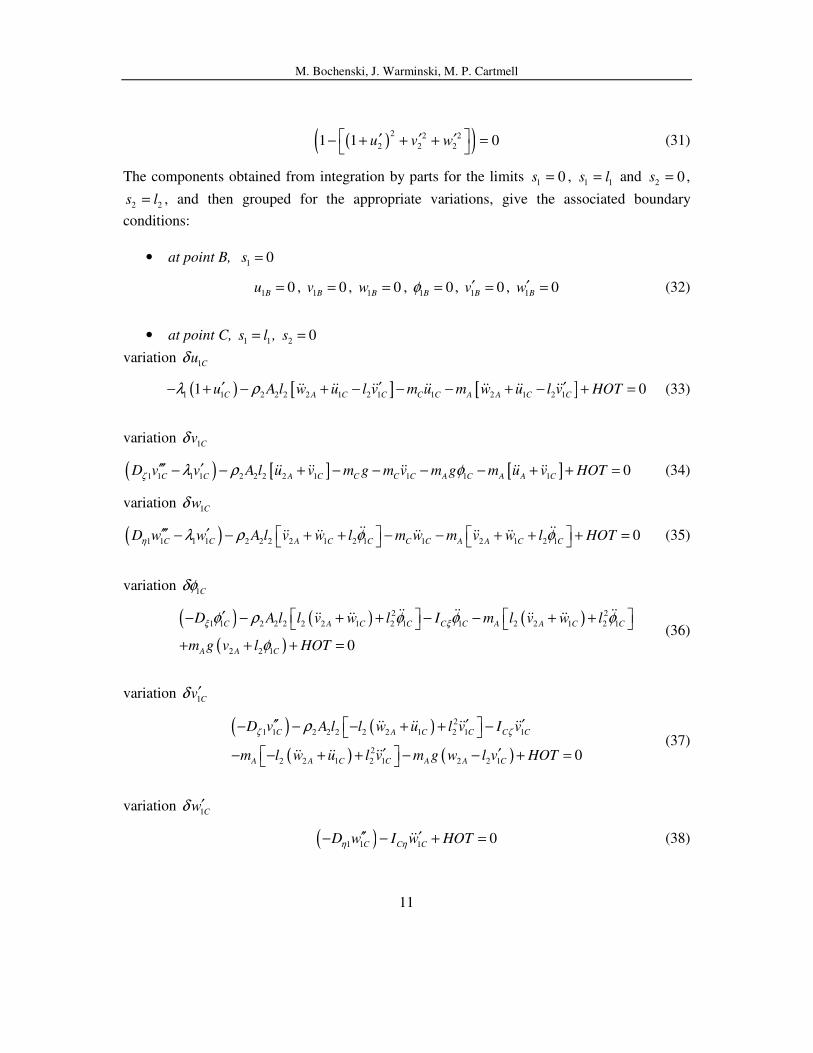
(31)

The components obtained from integration by parts for the limits 1 0s = ,

1 1s l= and 2 0s = ,

2 2s l= , and then grouped for the appropriate variations, give the associated boundary

conditions:

• at point B, 1 0s =

1 0Bu = ,

1 0Bv = , 1 0Bw = ,

1 0Bφ = , 1 0Bv′ = ,

1 0Bw′ = (32)

• at point C, 1 1s l= ,

2 0s =

variation 1Cuδ

( ) [ ] [ ]1 1 2 2 2 2 1 2 1 1 2 1 2 11 0C A C C C C A A C Cu A l w u l v m u m w u l v HOTλ ρ′ ′ ′− + − + − − − + − + =&& && && && && && && (33)

variation 1Cvδ

( ) [ ] [ ]1 1 1 1 2 2 2 2 1 1 1 10

C C A C C C C A C A A CD v v A l u v m g m v m g m u v HOTζ λ ρ φ′′′ ′− − + − − − − + + =&& && && && && (34)

variation 1Cwδ

( )1 1 1 1 2 2 2 2 1 2 1 1 2 1 2 10

C C A C C C C A A C CD w w A l v w l m w m v w l HOTη λ ρ φ φ ′′′ ′− − + + − − + + + =

&& &&&& && && && && (35)

variation 1Cδφ

( ) ( ) ( )

( )

2 2

1 1 2 2 2 2 2 1 2 1 1 2 2 1 2 1

2 2 1 0

C A C C C C A A C C

A A C

D A l l v w l I m l v w l

m g v l HOT

ξ ξφ ρ φ φ φ

φ

′− − + + − − + +

+ + + =

&& && &&&& && && && (36)

variation 1Cvδ ′

( ) ( )

( ) ( )

2

1 1 2 2 2 2 2 1 2 1 1

2

2 2 1 2 1 2 2 1 0

C A C C C C

A A C C A A C

D v A l l w u l v I v

m l w u l v m g w l v HOT

ζ ζρ′′ ′ ′ − − − + + −

′ ′ − − + + − − + =

&& && && &&

&& && &&

(37)

variation 1Cwδ ′

( )1 1 10

C C CD w I w HOTη η

′′ ′− − + =&& (38)


12

• at point A, 2 2s l=

variation 2 Auδ

( ) [ ]2 2 2 2 11 0A A A A Cu l m g m u v HOTλ ′− + − − + + =&& && (39)

variation 2 Avδ

( )2 2 2 2 1 2 1 2 10

A A A C A A C CD v v m g m v w l HOTζ λ φ φ ′′′ ′− − − + + + =

&&&& && (40)

variation 2 Awδ

( ) [ ]2 2 2 2 1 2 1 2 10

A A A C A A C CD w w m gv m w u l v HOTη λ′′′ ′ ′ ′− − − + − + =&& && && (41)

variation 2 Aδφ

( )2 2 20

A A AD I HOTξ ξφ φ′− − + =&& (42)

variation 2 Avδ ′

( )2 2 20

A A AD v I v HOTζ ζ

′′ ′− − + =&& (43)

variation 2 Awδ ′

( )2 2 20

A A AD w I w HOTη η

′′ ′− − + =&& (44)

Formulae for boundary conditions are given up to the first order terms while the second and

third orders are written by the abbreviation HOT, that means higher order terms. Indexes A, B,

C denote values at proper points. Note that to have consistency in Eqs. (33)-(38) variations of

the secondary beam at point s2=0 are expressed by variations of the primary beam at s1=l1, by

using a transformation of the local to the absolute set of coordinates.

The derived partial differential equations which describe the problem consist of the

geometrical and inertial nonlinear terms and nonlinear, non-homogenous, dynamical boundary

conditions. To solve this set of nonlinear equations of motion, and the nonlinear boundary

conditions, an approximate solution method has to be applied. It requires an appropriate

assumption for the admissible vibration modes which will then satisfy the boundary

conditions to the required perturbation order accuracy. This will be completed in further

analytical investigations of this problem, to be undertaken in the very near future. However, to

make proper assumptions for this further work on an approximate analytical approach

experimental and numerical (FEA) tests have been undertaken and these are presented in the

next section.


13

4 EXPERIMENT

The experimental setup used for the testing work is composed of a high end proprietary

modal analysis system, spectral acquisition software, and an electrically matched shaker with

feedback loop control of the excitation level. The signals are measured by three small, low

mass, piezo-sensors and a piezo-sensor is used for monitoring the excitation. The arrows in

Fig. 1 indicate the orientations of the sensors used in the experimental tests.

Preliminary experimental investigations consisted of tuning the structure for chosen

bending and torsional natural frequencies of the system. The frequencies are determined by

modal analysis of the system response activated by an impact. By modification of lumped

masses A and C and the length of the primary beam, the system has been tuned for a 1:4 ratio

of the first bending frequency of the primary beam ( )( )13.61

b IHzω = and the first bending

frequency of the secondary beam ( )( )114.45

b IIHzω = . The torsional frequency of the primary

beam, when the whole structure is fixed, has also been measured ( )( )1~ 4.9

t IHzω = . The

parameters of the tuned structure are listed in Table 1.

length of horizontal beam 236 mm

length of vertical beam 201 mm

mass A value 15.3 gr

mass C value 38.0 gr

Table 1. Parameters for structure after tuning 1:4

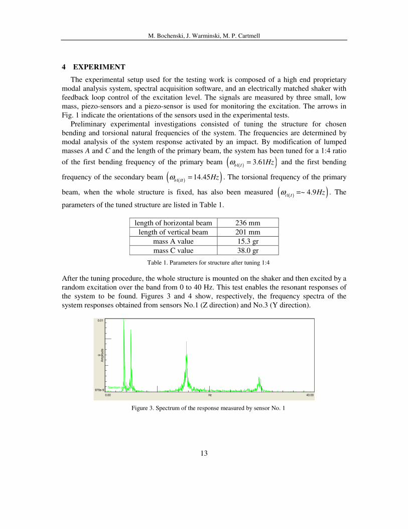
After the tuning procedure, the whole structure is mounted on the shaker and then excited by a

random excitation over the band from 0 to 40 Hz. This test enables the resonant responses of

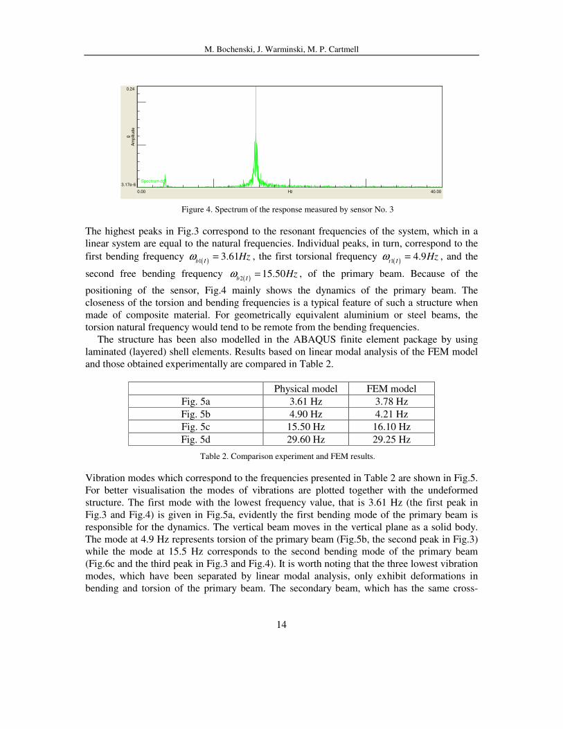
the system to be found. Figures 3 and 4 show, respectively, the frequency spectra of the

system responses obtained from sensors No.1 (Z direction) and No.3 (Y direction).

0.00 40.00 Hz

970e-9

0.01

Am

plit

ud

eg

Spectrum gora_bok

Figure 3. Spectrum of the response measured by sensor No. 1


14

0.00 40.00 Hz

3.17e-6

0.24

Am

plit

ude

g

Spectrum dol

Figure 4. Spectrum of the response measured by sensor No. 3

The highest peaks in Fig.3 correspond to the resonant frequencies of the system, which in a

linear system are equal to the natural frequencies. Individual peaks, in turn, correspond to the

first bending frequency ( )13.61

b IHzω = , the first torsional frequency ( )1

4.9t I

Hzω = , and the

second free bending frequency ( )215.50

b IHzω = , of the primary beam. Because of the

positioning of the sensor, Fig.4 mainly shows the dynamics of the primary beam. The

closeness of the torsion and bending frequencies is a typical feature of such a structure when

made of composite material. For geometrically equivalent aluminium or steel beams, the

torsion natural frequency would tend to be remote from the bending frequencies.

The structure has been also modelled in the ABAQUS finite element package by using

laminated (layered) shell elements. Results based on linear modal analysis of the FEM model

and those obtained experimentally are compared in Table 2.

Physical model FEM model

Fig. 5a 3.61 Hz 3.78 Hz

Fig. 5b 4.90 Hz 4.21 Hz

Fig. 5c 15.50 Hz 16.10 Hz

Fig. 5d 29.60 Hz 29.25 Hz

Table 2. Comparison experiment and FEM results.

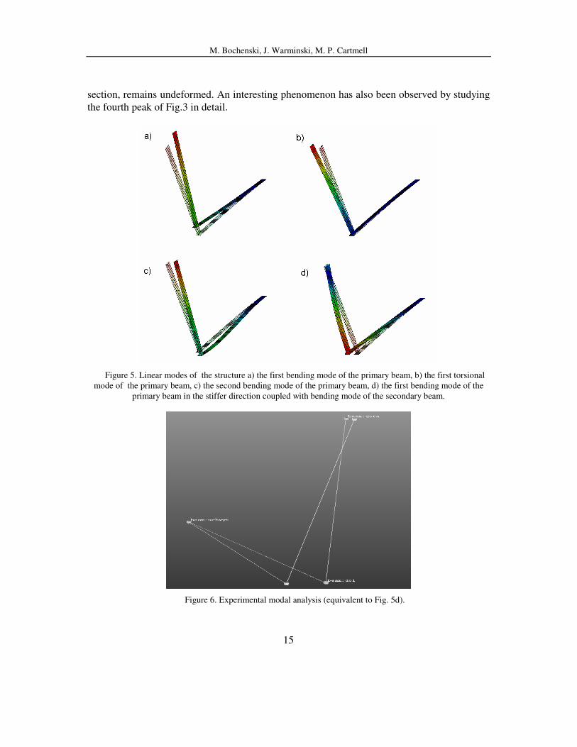
Vibration modes which correspond to the frequencies presented in Table 2 are shown in Fig.5.

For better visualisation the modes of vibrations are plotted together with the undeformed

structure. The first mode with the lowest frequency value, that is 3.61 Hz (the first peak in

Fig.3 and Fig.4) is given in Fig.5a, evidently the first bending mode of the primary beam is

responsible for the dynamics. The vertical beam moves in the vertical plane as a solid body.

The mode at 4.9 Hz represents torsion of the primary beam (Fig.5b, the second peak in Fig.3)

while the mode at 15.5 Hz corresponds to the second bending mode of the primary beam

(Fig.6c and the third peak in Fig.3 and Fig.4). It is worth noting that the three lowest vibration

modes, which have been separated by linear modal analysis, only exhibit deformations in

bending and torsion of the primary beam. The secondary beam, which has the same cross-


15

section, remains undeformed. An interesting phenomenon has also been observed by studying

the fourth peak of Fig.3 in detail.

Figure 5. Linear modes of the structure a) the first bending mode of the primary beam, b) the first torsional

mode of the primary beam, c) the second bending mode of the primary beam, d) the first bending mode of the

primary beam in the stiffer direction coupled with bending mode of the secondary beam.

Figure 6. Experimental modal analysis (equivalent to Fig. 5d).


16

For this frequency the bending mode of the vertical beam is excited, and, due to interaction,

the bending mode of the horizontal beam in the stiff direction is excited too. This out-of-plane

motion is presented in Fig.5d and is confirmed experimentally in Fig.6.

In many practical engineering applications, the control of motion of the top mass A plays

an important role. Therefore, the influence of the internal resonance conditions on trajectories

at this point is of interest. By imposing harmonic excitations at different frequencies, in

particular around the resonant areas, the response of the system can be investigated in some

detail. In this paper we only consider the resonant response around the torsional frequency of

the primary beam. This resonance has not been taken into account in the literature to date, to

the authors’ knowledge. To avoid damage to the structure, and to get satisfactory signals, the

amplitude of excitation has been carefully chosen. Fig.7 shows trajectories of the top mass

near the torsional resonance of the primary beam. The trajectories are reconstructed by signals

received from sensors No.1 and 2.

Figure 7. Trajectories of the top mass.

During transition through the resonance, differences in the structural response are clearly

visible. Inside the resonance area, near 4.9 Hz, the major axis of an elliptic trajectory is almost

parallel to the Z coordinate. Outside this resonance zone the axis rotates in the clockwise

direction and the trajectory, because of nonlinear interactions with other vibrations modes,

assumes a more complex shape, reminiscent of a Lissajous figure.


17

5 CONCLUSIONS AND FINAL REMARKS

The paper deals with preliminary theoretical and well developed experimental studies

of an autoparametric beam structure with essentially different stiffnesses in two

orthogonal directions. The systematically derived equations of motion, and the associated

dynamical boundary conditions, show that nonlinear terms which couple the structure

may result in many unexpected responses. An experimentally tested composite beam

structure, tuned for the 1:4 internal resonance condition, exhibits possible vibrations as an

out-of-plane motion in the stiff direction of the primary beam. In the neighbourhood of

the torsional resonance, due to nonlinear coupling, additional nonlinear modes are

involved in the system response, and this is expressed by the complex trajectories that

have been seen. The experimental work has confirmed the FEA analysis, with generally

very good agreement. Therefore the results give a promising basis for finding and

interpreting analytical solutions of the mathematical model, as summarised in section 3.

This, and further investigation will eventually allow a strategy to be developed for the

active control of this kind of structure by the application of PZT or SMA elements.

Acknowledgments

The work is supported by grants N502 049 31/1449 and 65/6.PR UE/2005/7 from the

Polish Ministry of Science and Higher Education. The authors would like to thank

Professor Ivelin Ivanov for his support with the FE modelling work, and for various

discussions and suggestions during the course of the research.

(1) This paper is based on final degree work undertaken during the Smart Technology Expert

School, Institute of Fundamental Technological Research, Warsaw, Poland.

REFERENCES

[1] A. H. Nayfeh and P. F. Pai, Linear and Nonlinear Structural Mechanics, Wiley-

Interscience, New York (2004).

[2] A. H. Nayfeh, Nonlinear Interactions, Wiley, New York (2000).

[3] M. R. M. Crespo da Silva and C. C. Glynn, Nonlinear flexural-flexural-torsional

dynamics of inextensional beams, Part I, “Equations of motion”, Journal of Structural

Dynamics, 6(4), 437-448 (1978).

[4] Crespo da Silva, M. R. M. and Glynn, C. C., Nonlinear flexural-flexural-torsional

dynamics of inextensional beams, Part II, Forced Motions, Journal of Structural

Dynamics, 6(4), 449-461, 1978.

[5] M. P. Cartmell, Simultaneous combination resonances in a parametrically excited

cantilever beam, Strain, 117-126 (1987).

[6] H. N, Arafat, A. H. Nayfeh and Char-Ming Chin, Nonlinear Nonplanar Dynamics of

Parametrically Excited Cantilever Beams, Nonlinear Dynamics, 15, 31–61 (1998).


18

[7] P. Malatkar, Nonlinear Vibrations of Cantilever Beams and Plates, PhD Thesis,

Blacksburg, Virginia (2003).

[8] A. Tondl, T. Ruijgrok, F. Verhulst, R. Nagergoj, Autoparametric Resonance in

Mechanical Systems, Cambridge University Press (2000).

[9] D. Sado, Energy transfer in nonlinearly coupled oscillators with two degrees of freedom,

(in Polish), Warsaw University of Technology Publisher, Mechanika, vol.166, Warsaw

(1997).

[10] B. Balachandran and A. H. Nayfeh, Nonlinear Motion of Beam-Mass Structure,

Nonlinear Dynamics, 1, 39-61, (1990).

[11] A. H. Nayfeh, B. Balachandran, and M. A. Collbert, An Experimental Investigation of

Complicated Responses of a Two-Degree-of-Freedom Structure, Transactions of the

ASME, Vol.56, 960-966 (1989).

[12] A. H. Nayfeh and L. D. Zavodney, Experimental Observation of Amplitude- and Phase-

modulated Responses of Two Internally Coupled Oscillators to a Harmonic Excitation,

Transactions of the ASME, Vol.55, 706-710 (1988).

[13] J. W. Roberts, M. P. Cartmell, Forced vibration of a beam system with autoparametric

coupling effects, Strain, 117-126 (1984).

[14] M. P. Cartmell and J. W. Roberts, Simultaneous combination resonances in an

autoparametricaly resonant system, Journal of Sound and Vibration, 123 (1), 81-101

(1988).

[15] M. P. Cartmell, The equations of motion for a parametrically excited cantilever beam,

Journal of Sound and Vibration, 143(3), 395-406 (1990).

[16] S. L. Bux and J. W. Roberts, Non-linear vibratory interactions in systems of coupled

beams, Journal of Sound and Vibration, 104(3), 497-520 (1986).

[17] D. I. M. Forehand and M. P. Cartmell, On the derivation of equations of motion of

parametrically excited cantilever beam, Journal of Sound and Vibration, 245(1), 165-

177, (2001).

[18] J. Warminski and M. Bochenski, Nonlinear vibrations of the autoparametrically coupled

beam structure, 8th Conference on Dynamical Systems – Theory and Applications, Lodz

827-832 (2005).

Documents

ANALYTICAL AND EXPERIMENTAL INVESTIGATIONS OF …smart.ippt.gov.pl/stec_graduates/stes_final_bochenski_marcin.pdf · 1 ANALYTICAL AND EXPERIMENTAL INVESTIGATIONS OF AN AUTOPARAMETRIC