Analytical and Experimental Investigations of Modified

Tuned Liquid Dampers (MTLDs)

by

Yongjian Chang

A thesis submitted in conformity with the requirements

for the degree of Master of Applied Science

Department of Civil Engineering

University of Toronto

© Copyright by Yongjian Chang 2015

ii

Analytical and Experimental Investigations of Modified

Tuned Liquid Dampers (MTLDs)

Yongjian Chang

Master of Applied Science

Department of Civil Engineering

University of Toronto

2015

Abstract

Tuned Liquid Dampers (TLDs), as passive control devices, have been used in high-rise

buildings for vibration control. A TLD dissipates energy through the sloshing of the water

inside the tank. Modified Tuned Liquid Damper (MTLD) utilizes the rotational spring

system at the base, therefore the MTLD experiences both horizontal and rotational

motions. In this study, MTLD-structure system subjected to sinusoidal excitation and

seismic events has been investigated using Lu’s analytical model. This analytical model

has been verified experimentally using Real-Time Hybrid Simulation method. The

important parameters of the MTLD including the dimensionless rotational stiffness

parameter, mass ratio, frequency ratio and damping ratio were studied in detail; and a

preliminary design procedure was outlined.

iii

Acknowledgments

I would like to really appreciate my research supervisor, Professor Oya Mercan, who

provided me the most useful guidance, encouraged me and helped me to modify my thesis

with more patience. And most importantly, she offered me an opportunity to complete my

M.A.Sc Degree in one year. I am also grateful to my second reader, Professor Karl

Peterson, who spent time to review my thesis and gave me the most valuable comments

and suggestions during my defence.

I also would like to thank Professor Constantin Christopoulos, who provided Quanser

Shake table and working area for me to do my experimental tests. Furthermore, I am

grateful to Ali Ashasi Sorkhabi and Reza Mirza Hessabi, who helped me for theory and

shake table tests during my study.

Finally, I really appreciate my parents who are always supporting me and encouraging me

during my life.

iv

Table of Contents

Table of Contents

Acknowledgments ............................................................................................................. iii

Table of Contents ............................................................................................................... iv

List of Tables .................................................................................................................... vii

List of Figures .................................................................................................................. viii

Chapter 1 ............................................................................................................................. 1

Introduction................................................................................................................. 1

1.1 Seismic Protection Systems ................................................................................. 1

1.1.1 Conventional Systems .................................................................................. 1

1.1.2 Seismic Isolation Systems ............................................................................ 1

1.1.3 Supplemental Damping Systems .................................................................. 2

1.2 Tuned Liquid Damper (TLD) .............................................................................. 4

1.2.1 History .......................................................................................................... 4

1.2.2 Tuned Liquid Dampers (TLDs) .................................................................... 5

1.2.3 Modified Tuned Liquid Dampers (MTLDs)................................................. 6

1.3 Scope of Study ..................................................................................................... 6

Chapter 2 ............................................................................................................................. 8

Literature Review ....................................................................................................... 8

2.1 Mathematical Models of TLD.............................................................................. 8

v

2.2 Different types of TLD ...................................................................................... 11

2.3 Modified Tuned Liquid Damper (MTLD) ......................................................... 13

2.4 Practical Implementation ................................................................................... 14

Chapter 3 ........................................................................................................................... 17

Theory and Analytical Model for Tuned Liquid Damper ........................................ 17

3.1 Governing Equation of TLD .............................................................................. 17

3.2 Numerical Solution Procedure ........................................................................... 20

3.3 TLD-Structure Interaction Configuration .......................................................... 21

3.4 MTLD-Structure Interaction Configuration ...................................................... 22

3.5 Solution Procedure ............................................................................................. 24

Chapter 4 ........................................................................................................................... 26

Numerical and Experimental Investigation Results ................................................. 26

4.1 Real-Time Hybrid Simulation (RTHS) Testing Method ................................... 26

4.2 Experimental Set-Up .......................................................................................... 27

4.3 𝐷𝑅𝑆𝑃 (𝐿𝑠) Investigation ................................................................................... 30

4.4 Mass Ratio and Structural Damping Ratio ........................................................ 37

4.5 Experimental verification ................................................................................... 39

4.6 MTLD-Structure Subjected to Ground Motions ................................................ 45

4.7 Preliminary Design Procedure ........................................................................... 50

Design Procedure ...................................................................................................... 50

vi

Chapter 5 ........................................................................................................................... 52

Summary and Conclusion ......................................................................................... 52

𝐷𝑅𝑆𝑃 Investigation ...................................................................................................... 52

Mass Ratio and Damping Ratio .................................................................................... 53

Accuracy of Analytical model ...................................................................................... 53

Future work ................................................................................................................... 54

References......................................................................................................................... 55

Appendix A MatLab Code for Lu’s Analytical model ..................................................... 62

Appendix B List of Symbols ............................................................................................ 66

vii

List of Tables

TABLE 1: THE PROPERTIES OF MTLD-STRUCTURE SYSTEM FOR DRSP INVESTIGATION .. 32

TABLE 2: STRUCTURAL DISPLACEMENT REDUCTION, DAMPING RATIO = 1.2% ................ 38

TABLE 3: STRUCTURAL DISPLACEMENT REDUCTION, MASS RATIO = 2% ......................... 38

TABLE 4: CASES FOR EXPERIMENTAL VERIFICATION ........................................................ 39

TABLE 5: EXPERIMENTAL VERIFICATION FOR THE CASE OF WAVE BREAKING ................... 41

viii

List of Figures

FIGURE 1: THE DIMENSION OF A RECTANGULAR TLD ........................................................ 17

FIGURE 2: TLD UNDER BOTH HORIZONTAL AND ROTATIONAL MOTIONS............................ 18

FIGURE 3: SCHEMATIC OF SINGLE FRAME WITH TLD ........................................................ 22

FIGURE 4: SCHEMATIC OF SINGLE FRAME WITH IDEALIZED MTLD .................................. 23

FIGURE 5: SCHEMATIC OF SINGLE FRAME WITH PRACTICAL MTLD ................................. 24

FIGURE 6: FLOWCHART OF NUMERICAL SOLUTION PROCEDURE ....................................... 25

FIGURE 7: SCHEMATIC DIAGRAM OF REAL-TIME HYBRID SIMULATION METHOD ............. 27

FIGURE 8: QUANSER SHAKE TABLE ................................................................................... 28

FIGURE 9: SCHEMATIC REPRESENTATION OF THE EXPERIMENTAL SET-UP OF MTLD ....... 29

FIGURE 10: (A) A CLOSE-UP VIEW OF THE SPRING AND PIVOT CONNECTION, (B)

ASSEMBLED MTLD ................................................................................................... 29

FIGURE 11: THE EFFECTS OF SPRING DISTANCE ON STRUCTURAL DISPLACEMENT,

ALPHA=0.8 ................................................................................................................ 32

FIGURE 12: THE EFFECTS OF SPRING DISTANCE ON STRUCTURAL DISPLACEMENT, ALPHA=1

.................................................................................................................................. 32

FIGURE 13: THE EFFECTS OF SPRING DISTANCE ON STRUCTURAL DISPLACEMENT,

ALPHA=1.2 ................................................................................................................ 33

FIGURE 14: THE EFFECTS OF MTLDS WITH DIFFERENT SPRING DISTANCE ON STRUCTURE,

ALPHA=0.8 ................................................................................................................ 35

FIGURE 15: THE EFFECTS OF MTLDS WITH DIFFERENT SPRING DISTANCE ON STRUCTURE,

ALPHA=1 ................................................................................................................... 35

FIGURE 16: THE EFFECTS OF MTLDS WITH DIFFERENT SPRING DISTANCE ON STRUCTURE,

ALPHA=1.2 ................................................................................................................ 36

ix

FIGURE 17: DISPLACEMENT TIME HISTORY OF SINUSOIDAL EXCITATION, ALPHA=0.8,

BETA=1 ...................................................................................................................... 37

FIGURE 18: DISPLACEMENT TIME HISTORY OF SINUSOIDAL EXCITATION, ALPHA=1,

BETA=0.95 ................................................................................................................. 37

FIGURE 19: DISPLACEMENT TIME HISTORY, 𝐿𝑠=0.45M, BETA=1.05 .................................. 40

FIGURE 20: DISPLACEMENT TIME HISTORY, 𝐿𝑠=0.24M, BETA=1 ....................................... 40

FIGURE 21: DISPLACEMENT TIME HISTORY, 𝐿𝑠=0.2M, BETA=0.95 .................................... 40

FIGURE 22: DISPLACEMENT TIME HISTORY, 𝐿𝑠=0.45M, BETA=1.05 ................................. 42

FIGURE 23: DISPLACEMENT TIME HISTORY, 𝐿𝑠=0.36M, BETA=0.95 ................................. 43

FIGURE 24: DISPLACEMENT TIME HISTORY, 𝐿𝑠=0.2M, BETA=1 ........................................ 44

FIGURE 25: STRUCTURAL RESPONSE (NUMERICAL) WITH AND WITHOUT MTLD UNDER

KOBE EARTHQUAKE, ALPHA=0.8............................................................................... 45

FIGURE 26: STRUCTURAL RESPONSE (NUMERICAL) WITH AND WITHOUT MTLD UNDER

KOBE EARTHQUAKE, ALPHA=1.................................................................................. 46

FIGURE 27: STRUCTURAL RESPONSE WITH AND WITHOUT MTLD UNDER KOBE

EARTHQUAKE ............................................................................................................ 48

FIGURE 28: STRUCTURAL RESPONSE WITH AND WITHOUT TLD UNDER EI CENTRO

EARTHQUAKE ............................................................................................................ 49

FIGURE 29: FLOWCHART OR PRELIMINARY DESIGN PROCEDURE ...................................... 51

1

Chapter 1

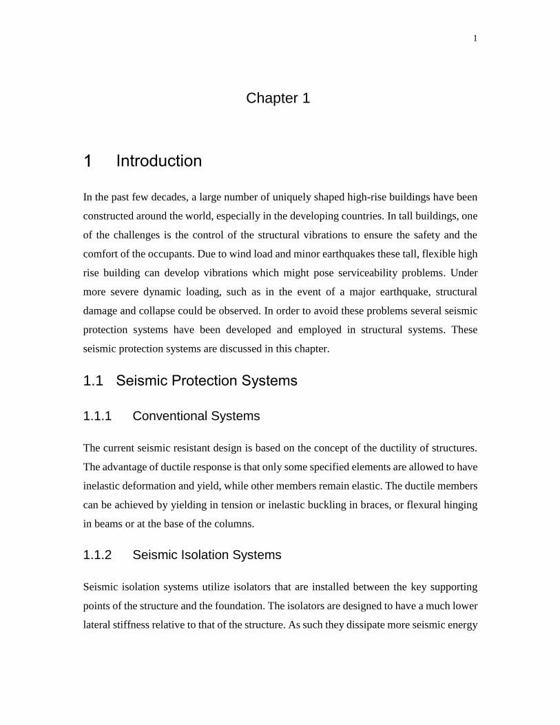
Introduction

In the past few decades, a large number of uniquely shaped high-rise buildings have been

constructed around the world, especially in the developing countries. In tall buildings, one

of the challenges is the control of the structural vibrations to ensure the safety and the

comfort of the occupants. Due to wind load and minor earthquakes these tall, flexible high

rise building can develop vibrations which might pose serviceability problems. Under

more severe dynamic loading, such as in the event of a major earthquake, structural

damage and collapse could be observed. In order to avoid these problems several seismic

protection systems have been developed and employed in structural systems. These

seismic protection systems are discussed in this chapter.

1.1 Seismic Protection Systems

1.1.1 Conventional Systems

The current seismic resistant design is based on the concept of the ductility of structures.

The advantage of ductile response is that only some specified elements are allowed to have

inelastic deformation and yield, while other members remain elastic. The ductile members

can be achieved by yielding in tension or inelastic buckling in braces, or flexural hinging

in beams or at the base of the columns.

1.1.2 Seismic Isolation Systems

Seismic isolation systems utilize isolators that are installed between the key supporting

points of the structure and the foundation. The isolators are designed to have a much lower

lateral stiffness relative to that of the structure. As such they dissipate more seismic energy

2

and transfer less energy into the structure. In general, seismic isolation systems have three

main types: laminated-rubber bearings, lead-rubber bearings and the friction pendulum

systems.

1.1.3 Supplemental Damping Systems

Supplemental damping devices are introduced into the structure to dissipate some of the

energy introduced during the vibration and thereby mitigate the damage to the structural

and non-structural components. They can be classified in three categories as, active, semi-

active and passive systems.

1.1.3.1 Active Systems

Active systems monitor the state of structure by using the data acquired from sensors

placed on the structure. They determine the action that needs to be taken in order to

mitigate the dynamic response and then apply the required forces to the structure to modify

its current state. Under dynamic loading all these steps need to be completed in a short

time and require a continuous external power source especially to introduce the control

forces. However, during a severe earthquake the power source might be lost, and as a result

the active systems might stop functioning. For that reason active systems are not preferred

as the seismic protective systems for civil structures.

1.1.3.2 Semi-Active Systems

Semi-active systems, unlike the active control systems, only need a small amount of

external power. They do not apply the external forces to the structure, but semi-active

control systems modify the structural properties, such as the damping as the structure

vibrates. Magneto-rheological dampers can be given as an example for semi-active control

systems.

3

1.1.3.3 Passive Systems

Unlike active and semi-active systems, passive systems do not need external power,

monitoring systems, sensors and actuators. Properties of passive systems are fixed and they

are not get modified during the vibration of the structure. Passive systems are considered

to be an effective, robust and economical solution, and they have been already

implemented in a variety of civil structures. Passive systems can be divided into three

categories: displacement-activated, velocity-activated and motion-activated.

Metallic dampers, friction dampers, self-centering dampers and viscoelastic dampers

belong to the group of displacement-activated devices. They absorb seismic energy

through the relative displacement between their contact points that are connected to the

structure. Metallic dampers absorb seismic energy by their hysteretic behaviour when they

deform into the post-elastic range. Friction dampers dissipate energy by friction caused by

the sliding motion of two solid surfaces in contact.

Viscous and viscoelastic dampers belong to the group of velocity-activated devices. They

dissipate energy through the relative velocity between their connection points. The

behaviour of dampers are dependent on velocity and frequency of the motion and are out

of phase with the maximum internal forces generated by the peak deformation of structure.

Lower design forces might be required for the structural members when this type of

dampers are employed.

Tuned Mass Damper (TMD) and Tuned Liquid Damper (TLD) belong to the group of

motion-activated devices. These dampers have their own period that need to be tuned to

the fundamental structural period. They are typically placed on the top of the structure.

The details of TLDs are discussed in the next section.

4

1.2 Tuned Liquid Damper (TLD)

1.2.1 History

The first application of Tuned Liquid dampers was in space satellites (Bhuta, 1966) and

marine vessels (Watanabe, 1969). Around ten years later, the dampers were employed in

the offshore platforms and ground structures (Vandiver, 1978 and Lee, 1982). Modi (1987)

and Welt (1988) developed parametric study on the annular TLD, and showed that this

damper can be effective for civil structures. In the late 1980s, liquid dampers have been

used in tall towers in Japan, such as the Haneda Airport Tower, the Narita Airport Tower

(Tamura et al., 1992) and Shin Yokohama Prince (SYP) Hotel in Yokohama (Wakahara

et al., 1992), and also on bridges such as the Ikuchi Bridge and the Sakitama Bridge in

Japan (Kaneko and Ishikawa 1999).

The first nonlinear model of a rectangular TLD was developed by Shimizu and Hayama

(1987), where the model combines the shallow water wave theory with the potential flow

theory. Later, Sun et al. (1989) improved the model for harmonic motion and by

accounting for the wave breaking with the introduction of two empirical parameters.

Response to random input was studied in Koh et al.’s extended work (Koh et al., 1994).

Kubo et al. (1989) first developed a preliminary experimental study to investigate the

effectiveness of rectangular TLDs in controlling the pitching vibration of structure. Then

Kotsubo et al. (1990) produced an equivalent mechanical model of the TLD that predicts

the sloshing forces and moments caused by the sloshing water under pitching motion,

however, the sloshing damping was not considered. Based on these two papers, Sun et al.

(1995) developed a numerical model for rectangular TLDs under purely pitching motion

based on the non-linear shallow water wave theory where linear damping was considered.

Lu (2001) created a new numerical model by using classical shallow water theory with an

improved boundary shear model to simulate the sloshing of a liquid in a rectangular TLD

that experiences combined horizontal and rotational motion. Samanta and Banerji (2008)

numerically investigated the dynamic behaviour of a structure equipped with Modified

5

Tuned Liquid Damper (MTLD) under harmonic motions by using Lu’s model. A MTLD

can move in both horizontal and rotational motion on the top of structure.

1.2.2 Tuned Liquid Dampers (TLDs)

Tuned Liquid Dampers (TLDs) are passive energy absorbing devices that have been used

especially in some flexible, high-rise buildings to control the vibrations. They are typically

rectangular tanks partially filled with water that are installed on the roof of the structures.

The sloshing TLD absorbs and dissipates energy through boundary layer friction, wave

breaking and free-surface contamination (Fujino et al., 1992). Based on the ratio of water

depth (i.e, height) to length of tank (ℎ/𝐿), TLD can be divided into two categories, shallow

water dampers (ℎ/𝐿 < 0.15) and deep water dampers (ℎ/𝐿 > 0.15) (Banerji et al., 2000).

An important parameter of TLD is the water sloshing frequency. By tuning the sloshing

frequency to the natural frequency of structure, a significant amount of sloshing and wave

breaking can be activated. Thereby a considerable amount of vibration energy can be

dissipated at resonant frequency (Sun et al., 1992). Malekghasemi (2011) suggested that

the TLD can remain effective as long as the ratio of natural frequency of structure to

sloshing frequency of TLD is in the range of 1 to 1.2. In addition, the mass ratio is also an

important parameter of TLD. Banerji et al. (2000) indicated that the structure vibration

control is more effective if the mass ratio is in the range of 1% to 4%.

TLDs have some advantages compared to other passive systems. (i) They are cost-effective

and are easy to install and maintain; (ii) It is easy to tune their sloshing frequency by

changing the water level or the tank dimensions; (iii) They are effective under small

amplitude vibrations and for a wide range of excitation frequencies (Sun et al. 1992); (iv)

They can be tuned along two orthogonal directions; (v) They can act as a fire-extinguishing

system during fire emergencies.

6

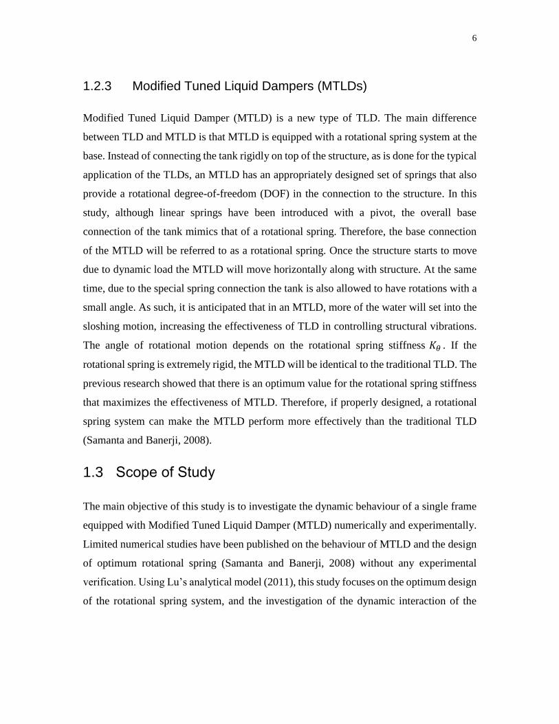
1.2.3 Modified Tuned Liquid Dampers (MTLDs)

Modified Tuned Liquid Damper (MTLD) is a new type of TLD. The main difference

between TLD and MTLD is that MTLD is equipped with a rotational spring system at the

base. Instead of connecting the tank rigidly on top of the structure, as is done for the typical

application of the TLDs, an MTLD has an appropriately designed set of springs that also

provide a rotational degree-of-freedom (DOF) in the connection to the structure. In this

study, although linear springs have been introduced with a pivot, the overall base

connection of the tank mimics that of a rotational spring. Therefore, the base connection

of the MTLD will be referred to as a rotational spring. Once the structure starts to move

due to dynamic load the MTLD will move horizontally along with structure. At the same

time, due to the special spring connection the tank is also allowed to have rotations with a

small angle. As such, it is anticipated that in an MTLD, more of the water will set into the

sloshing motion, increasing the effectiveness of TLD in controlling structural vibrations.

The angle of rotational motion depends on the rotational spring stiffness 𝐾𝜃 . If the

rotational spring is extremely rigid, the MTLD will be identical to the traditional TLD. The

previous research showed that there is an optimum value for the rotational spring stiffness

that maximizes the effectiveness of MTLD. Therefore, if properly designed, a rotational

spring system can make the MTLD perform more effectively than the traditional TLD

(Samanta and Banerji, 2008).

1.3 Scope of Study

The main objective of this study is to investigate the dynamic behaviour of a single frame

equipped with Modified Tuned Liquid Damper (MTLD) numerically and experimentally.

Limited numerical studies have been published on the behaviour of MTLD and the design

of optimum rotational spring (Samanta and Banerji, 2008) without any experimental

verification. Using Lu’s analytical model (2011), this study focuses on the optimum design

of the rotational spring system, and the investigation of the dynamic interaction of the

7

MTLD-structure system for a wide range of excitation frequencies. It also provides

experimental validation using real-time hybrid simulation (RTHS).

Chapter 2 outlines the literature review.

Chapter 3 presents the theory and the analytical model. Lu’s model is utilized in this study.

The explanation of Lu’s model is outlined and the details of model are discussed. The

effects of rotational spring system on the response of the MTLD are considered.

Chapter 4 introduces the experimental set-up and describes the real-time hybrid simulation

method employed. The results of the numerical simulations are provided and the

experimental results are presented to verify the numerical results. In addition, a preliminary

design procedure is outlined.

Chapter 5 provides summary and conclusions of this study together with some suggestions

of future work.

8

Chapter 2

Literature Review

In the past few decades a large number of papers have been published on the study different

kinds of TLDs with both numerical analysis and experimental testing components. The

different shapes of TLD have been investigated include rectangular and circular tanks.

Also, several researchers have established the different mathematical models to describe

the behaviour of the water tank, and compared the results with those obtained from

experimental tests.

2.1 Mathematical Models of TLD

Shimizu and Hayama (1987) derived the basic equations that describe the nonlinear

response of sloshing water in the rectangular tank under horizontal motion using the

shallow water wave theory with potential flow theory. They used the Runge-Kutta-Gill

Method to solve the ordinary differential equations of time and determined the damping

provided by the liquid through experimental testing. Shimizu and Hayama (1989) also

investigated the numerical model for circular TLDs.

Similar to the model of Shimizu and Hayama, Sun et al. (1989) developed a mathematical

model based on the nonlinear shallow water wave theory to describe the liquid motion in

a rectangular tank. But they improved the model by introducing a semi-analytical method

for the liquid damping due to the friction of boundary shear. They investigated TLD

experimentally by using a shaking table to compare with the simulation results, which

showed a good agreement with small oscillation amplitude excitation, up to 10mm. In these

tests no wave breaking wave was observed for the tank with the size of 590mm length,

335mm width and 30mm water height.

9

In order to account for the effect of breaking waves, Sun et al. (1991) improved the

mathematical model by introducing two empirical coefficients identified experimentally,

one is damping coefficient of liquid Cda, and another one is the wave phase velocity Cfr.

The model was verified experimentally and it was confirmed that the behaviour of water

tank can be predicted, and even the occurrence of wave breaking.

Sun et al. (1995) developed a model with equivalent mass, stiffness, and damping of the

TLD using Tuned Mass Damper (TMD) analogy from experimental data of rectangular,

circular and annular tanks subjected to harmonic base excitation.

Koh et al. (1994) studied the behaviour of rectangular TLDs under arbitrary excitation.

They used an existing model where the energy dissipation was included by liquid viscosity.

The results showed that the liquid motion was depended on the sloshing frequency,

amplitude and frequency content of the excitation.

Yu et al. (1997) used a different way to model TLD by treating TLD as an equivalent tuned

mass damper with nonlinear stiffness and damping. The model can be used to describe the

behaviour of TLD under a wide range of excitation amplitude.

Reed et al. (1998) investigated the TLDs by focusing on the large amplitude excitation up

to 40mm, with numerical modelling and experimental testing. The authors used the

random-choice numerical method to solve the nonlinear shallow water wave equation. In

the experimental test, they investigated the TLD in terms of the sloshing force, liquid

surface height and the energy dissipation. This paper included the tests for a tank with

590mm length, 335mm width and 30mm height of water, and subjected to excitation

amplitude with 10mm, 20mm and 40mm. But in their numerical analyses, they only

showed the results for the excitation amplitude of 20mm, which had a good agreement

between the experimental and the numerical results. The results also showed that the

increased excitation amplitude will increase the response frequency of TLD. Reed et al.

suggested that the sloshing frequency of TLD should be tuned to the frequency of structure

to have the damper perform better.

10

Banerji et al. (2000) used Sun’s model to simulate the Single-Degree-of-Freedom (SDOF)

structure with fixed-bottom TLD, subjected to real and artificial ground motions. They

investigated the parameters of TLD, including the ratio of the sloshing frequency to the

fundamental frequency of the structure, the ratio of the water mass to the structural mass

and the ratio of the depth of water to the length of tank, which are the important parameters

that influence the effectiveness of TLDs in reducing the vibrations. In 2002, Banerji et al.

carried out an experimental study to verify the numerical results and found out that Sun’s

model could not accurately capture the response of the TLD-structure system. Therefore,

in 2006, Samanta and Banerji employed another mathematical model developed by Lu

(2001) to simulate the behaviour of TLD-structure system subjected to large amplitude

base motion, and obtained better results than those obtained from Sun’s model.

Lee et al. (2007) employed the Real-Time Hybrid Simulation (RTHS) method to

investigate the performance of TLD. They tested the TLD physically as experimental

substructure and modeled a structure in computer as analytical substructure, then verified

the results with those from a shake table test. They indicated that the RTHS method can

evaluate the behaviour of TLD-structure system accurately.

Malekghasemi (2011) used real-time hybrid simulation method to experimentally test the

TLD-structure system by using shake table. In this study the TLD was physically tested

and the structure was analytically modeled in a computer. The whole system was subjected

to a sinusoidal force and three ground motions. Malekghasemi (2011) studied the effects

of different parameters, including mass ratio, frequency ratio and damping ratio and

investigated the accuracy of three simplified mathematical models, namely, Sun’s model,

Yu’s model and Xin’s model using the experimental results from RTHS. The results

showed that the TLD is most efficient when the frequency ratio is between 1 and 1.2 and

the mass ratio is 3%.

11

2.2 Different types of TLD

Modi et al. (1990) studied the energy dissipation and damping introduced by liquid

sloshing motion in torus shaped dampers analytically and experimentally. The authors also

investigated the wind induced instability of the damper, including vortex and galloping

response and concluded that the torus shaped damper is an effective device to control the

vibrations.

Modi and Seto (1997) investigated the rectangular nutation damper for the suppression of

wind-excited oscillations of structures. The study included the investigation of system

parameters that improve the performance of nutation damper, and the effectiveness of

nutation damper introduced to tall buildings by wind tunnel experiments.

Modi and Munshi (1998) improved the rectangular liquid damper by putting two

semicircular obstacles at the bottom of the tank to increase the energy dissipation. They

investigated the optimum size and location of these obstacles by using wind tunnel tests to

evaluate the effectiveness of the improved damper. Compared to the original damper, it

was shown that the improved damper had up to 60% more energy dissipation.

Modi and Akinturk (2002) used the same method as Modi and Munshi (1998), to study a

new type of liquid damper with wedge-shaped obstacles instead of semicircular obstacles.

This new investigation focused on the three different type of wedges, two smooth wedges,

one smooth wedge and one wedge with steps and two wedge with holes. Again, the

efficiency of the damper and the energy dissipation characteristics were evaluated. The

results showed that the optimum configuration can improve the energy dissipation.

Furthermore, Modi et al. (2003) investigated the influence of floating particles used in the

rectangular damper with wedge-shaped obstacles, 40% improvement was obtained in

comparison with the water-only case.

Followed by Gardarsson et al., Olson and Reed (2001) further investigated the TLD with

a sloped bottom of 30° by using Yu’s model, and compared the behaviour with that of

12

box-shaped TLD. They indicated that the sloped-bottom tank can be described by a

softening spring. They also suggested that in order to get the maximum effectiveness, the

sloshing frequency of tank should be slightly higher than the natural frequency of the

structure.

Xin et al. (2009) investigated a density-variable TLD with sloped bottom on a three-story

structure. They observed that the density-variable TLD with sloped bottom performs more

effectively and more robust than a flat bottom TLD in reducing the story drift and

acceleration of structure.

Screens have been used in TLDs to increase the dissipated energy. Tait et al. (2005) used

both the linear and nonlinear numerical flow models to predict the behaviour of TLD

equipped with screens, subjected to both wind loading and earthquake motion and verified

by experimental tests.

Tait et al. (2005) published another paper that studied the behaviour of TLD equipped with

damping screen under 2D excitation. The authors employed the same nonlinear model used

in 1D-case to simulate the 2D TLD, by decoupling and treating the 2D TLD as two

independent 1D cases and super-positioning them together., then compared with

experimental test. The experimental tests were carried out using a shake table that can

excite the TLD in two independent perpendicular horizontal directions. The findings

showed that the response of 2D TLD can be analysed as two 1D TLD independently, and

also the 2D TLD can be used in controlling the vibration of a structure in two principle

directions.

Tait (2008) introduced an equivalent linear mechanical model which includes the factor of

energy dissipated caused by the damping screens, and carried out a verification study

experimentally. A preliminary design procedure for initial size of the TLD and the

damping screen configuration is included in this paper. Tait et al. (2011) investigated the

influence and efficiency of TLD equipped with inclined screens. They developed a

13

mathematical model and provided experimental validation for this new configuration as

well.

2.3 Modified Tuned Liquid Damper (MTLD)

Sun et al. (1995) investigated the behaviour of rectangular TLDs under pitching motion.

They modified the analytical model by replacing the acceleration of gravity 𝑔 with the

vertical acceleration 𝑎𝑦, which would change during pitching vibration. The comparison

with the experimental results under pitching motion showed that the model predictions

were accurate in a small amplitude range.

The numerical methods developed by previous researchers can only predict the behaviour

of TLD well under an excitation with amplitude up to 40mm. This is insufficient due to

the uncertainty associated with earthquake and wind loading. Therefore, Lu (2001)

developed a new numerical model by using the shallow water theory to simulate the liquid

sloshing in rectangular TLDs subjected to horizontal excitation combined with rotational

motion. He found that the equations in the numerical model is better to be solved by the

Lax Finite Difference Scheme method. In this method the parameter α can be chosen

empirically. It can be reduced to increase the numerical damping to cut off the high-

frequency peak during high excitations that may cause numerical instability. The results

showed that the rotation can increase the effectiveness of TLD significantly. The research

in this thesis used Lu’s model to simulate the motion of the modified TLD.

Based on Banerji et al.’s own previous research and Lu’s model (Lu 2001), Samanta and

Banerji (2009) introduced the modified TLD which is equipped with a rotational system

at its base. When excited horizontally at its base, the modified TLD exhibits both

translational (i.e., horizontal) and rotational motion. As such, An SDOF structure equipped

with the modified TLD has two degree of freedoms, one is the horizontal motion of the

structure at the roof and the other is the rotation motion of modified TLD. The results

showed that there is an optimum value for the rotational spring system which provides the

maximum the effectiveness for the modified TLD. Samanta and Banerji also showed that

14

the modified TLD performs similar to a standard (fixed bottom) TLD if the rotational

spring system at the base is rigid. However, Samanta and Banerji only provided the theory

and numerical analysis for Modified TLD, they did not perform experimental tests to verify

the feasibility of such analytical model. And also there is no other research paper focused

on the experimental verification. Therefore, this study is very significant to investigate the

behaviour of MTLD numerically and experimentally.

2.4 Practical Implementation

The nutation damper has been used in airport towers at the Haneda and Narita International

airport to suppress wind-induced vibration. Tamura et al. (1992) experimentally tested the

nutation damper combined with building model by small amplitude excitation. And also

they investigated the effectiveness of nutation damper applied to 18 degree-of-freedom

analytical model of Haneta Airport tower and 21 degree-of-freedom analytical model of

Narita airport tower, where the nutation damper was represented as Tuned Mass Damper

(TMD). The results shown the 55% reduction of acceleration response of the tower using

the nutation damper with 1% mass ratio and floating particles.

Wakahara et al. (1992) introduced an actual application of the TLD to a high-rise structure,

the Shin Yokohama Prince (SYP) Hotel in Yokohama, Japan. They developed a new

simulation method to account for the nonlinearity of TLD, which can predict the effects of

TLD on high-rise building effectively. In addition, they carried out the experimental test

to verify the designed optimum TLD for the tower.

Koh et al. (1994) studied the multiple-mode liquid dampers that applied to the suspension

bridge, Golden Gate Bridge, subjected to 3 types of earthquake excitation. The authors

employed Sun’s nonlinear numerical model to simulate three modes of TLD corresponding

to first three vibration modes of the bridge, which interact with the structure in terms of

three vibration modes by applying the multiple-TLD to the different position. The findings

showed that the multiple-mode liquid dampers can control the vibration of the bridge with

15

several frequencies better than one liquid damper could control the vibration with only one

frequency, as excited by different types of earthquake.

The first case of TLD application is installation Nagasaki Airport Tower (NAT), Nagasaki,

Japan, in 1987 (Tamura et al., 1995). The TLDs were temporarily installed on the NAT in

order to verify the effectiveness of TLD in reducing structural vibration. They found that

the decrease in amplitude of vibration is 44% while reduction in RMS displacement was

about 35% with the installation of 25 vessels of TLD.

The TLD has also been installed on Yokohama Marine Tower (YMT) in Japan (Tamura et

al., 1995). It was found that when the TLD was installed, the damping ratio was increased

to 4.5% from the original damping ratio of 0.6%. In addition, the maximum acceleration

was reduced from 0.27m/s2 to 0.1m/s2.

The TLDs were also applied on the Shin Yokohama Prince Hotel (SYPH) in Yokohama,

Japan (Tamura et al., 1995). The container has the diameter of 2m and the height of 0.22m,

and was located in multi-layer stack. Each stack has 9 circular containers and the total

height is 2m. It has been noticed that the TLD can reduce 30% of RMS accelerations (from

0.01m/s2 to 0.006m/s2) in each direction under wind load with the speed of 20m/s, which

satisfied the ISO minimum perception level at 0.31Hz.

Another case of TLD application was on The Tokyo International Airport Tower (TIAT)

in 1993 (Tamura et al., 1995). There are 1400 tanks filled with water and floating

polyethylene particles in order to enhance the energy dissipation. The container has the

diameter of 0.6m and elevation of 0.125m. The mass ratio of the total mass of TLDs and

the first modal mass of the tower is around 3.5%. And the sloshing frequency of TLD is

lightly lower than natural frequency of the tower. The results showed that the TLD can

reduce the 60% of the RMS acceleration response of the tower without TLD.

Novo et al. (2013) employed Finite Element Method to investigate the behaviour of an

isolated TLD subjected to sinusoidal force with different amplitudes. They also utilized

linear dynamic analysis to evaluate the efficiency of the LTD for modern architecture

16

buildings in southern European countries. They showed that TLD is efficient and can

significantly increase the energy dissipation and the equivalent damping of the structure.

17

Chapter 3

Theory and Analytical Model for Tuned Liquid

Damper

3.1 Governing Equation of TLD

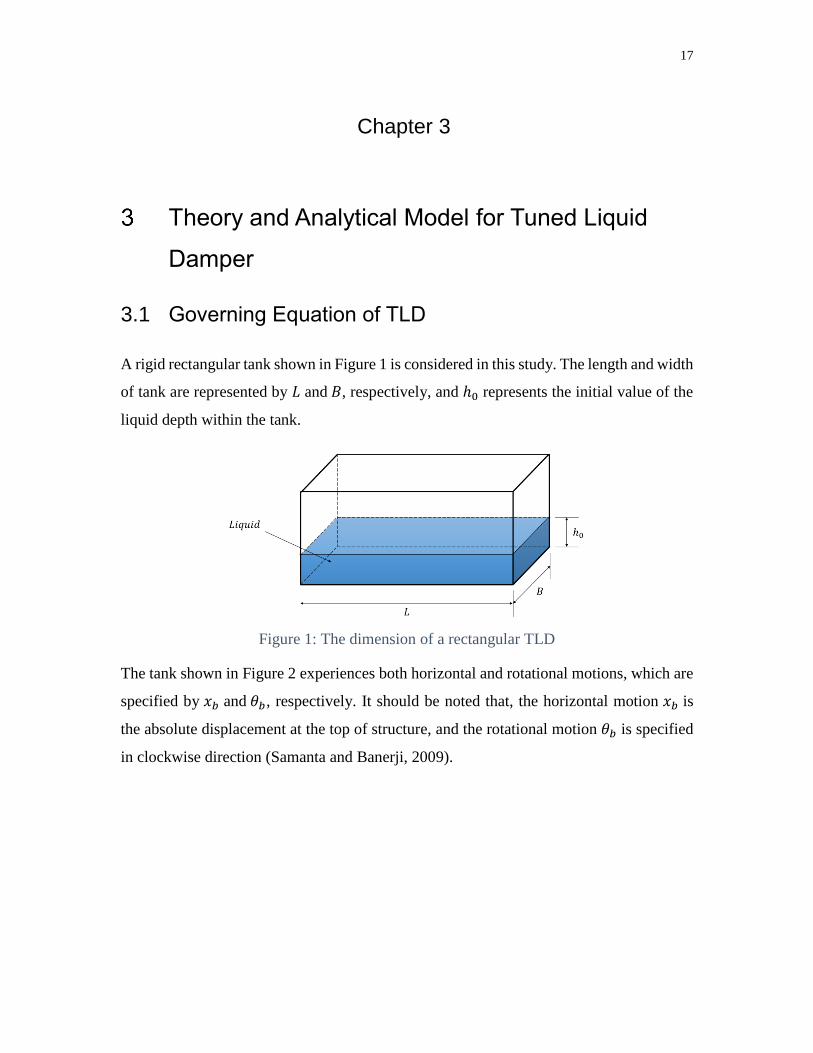
A rigid rectangular tank shown in Figure 1 is considered in this study. The length and width

of tank are represented by 𝐿 and 𝐵, respectively, and ℎ0 represents the initial value of the

liquid depth within the tank.

Figure 1: The dimension of a rectangular TLD

The tank shown in Figure 2 experiences both horizontal and rotational motions, which are

specified by 𝑥𝑏 and 𝜃𝑏, respectively. It should be noted that, the horizontal motion 𝑥𝑏 is

the absolute displacement at the top of structure, and the rotational motion 𝜃𝑏 is specified

in clockwise direction (Samanta and Banerji, 2009).

18

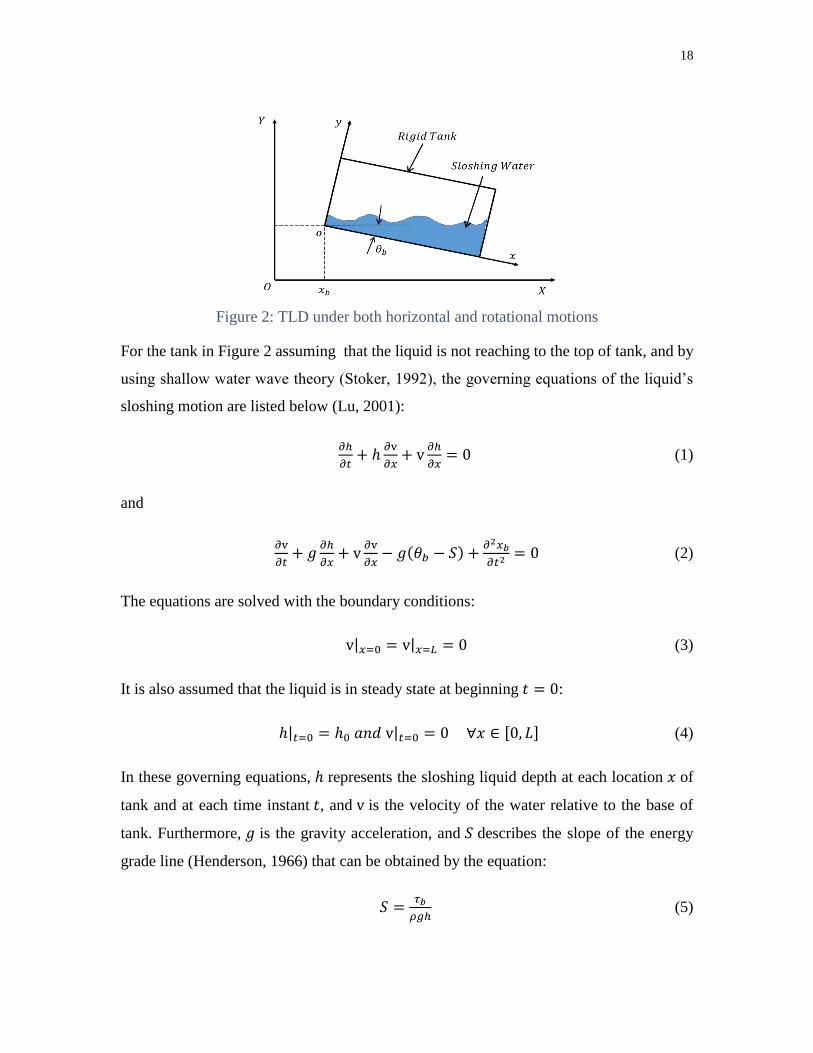
Figure 2: TLD under both horizontal and rotational motions

For the tank in Figure 2 assuming that the liquid is not reaching to the top of tank, and by

using shallow water wave theory (Stoker, 1992), the governing equations of the liquid’s

sloshing motion are listed below (Lu, 2001):

𝜕ℎ

𝜕𝑡+ ℎ

𝜕v

𝜕𝑥+ v

𝜕ℎ

𝜕𝑥= 0 (1)

and

𝜕v

𝜕𝑡+ 𝑔

𝜕ℎ

𝜕𝑥+ v

𝜕v

𝜕𝑥− 𝑔(𝜃𝑏 − 𝑆) +

𝜕2𝑥𝑏

𝜕𝑡2 = 0 (2)

The equations are solved with the boundary conditions:

v|𝑥=0 = v|𝑥=𝐿 = 0 (3)

It is also assumed that the liquid is in steady state at beginning 𝑡 = 0:

ℎ|𝑡=0 = ℎ0 𝑎𝑛𝑑 v|𝑡=0 = 0 ∀𝑥 ∈ [0, 𝐿] (4)

In these governing equations, ℎ represents the sloshing liquid depth at each location 𝑥 of

tank and at each time instant 𝑡, and v is the velocity of the water relative to the base of

tank. Furthermore, 𝑔 is the gravity acceleration, and 𝑆 describes the slope of the energy

grade line (Henderson, 1966) that can be obtained by the equation:

𝑆 =𝜏𝑏

𝜌𝑔ℎ (5)

19

Where, 𝜏𝑏 is the liquid’s shear stress at the base of tank and defined by:

𝜏𝑏 =𝜇v𝑚𝑎𝑥

ℎ 𝑓𝑜𝑟 𝑧 ≤ 0.7 (6a)

and

𝜏𝑏 = √𝜌𝜇𝜔v𝑚𝑎𝑥 𝑓𝑜𝑟 𝑧 > 0.7 (6b)

𝜌 and 𝜇 are representing the density and the dynamic viscosity of the liquid, respectively.

𝜇 is related to the kinetic viscosity 𝑣 by the equation:

𝜇 = 𝜌𝑣 (7)

Furthermore, 𝜔 is the excitation circular frequency, and the liquid’s dimensionless depth

𝑧 is introduced by Lu (2001):

𝑧 = √𝜔𝑔

2𝜇ℎ (8)

An important parameter in equation 6 is v𝑚𝑎𝑥 , the maximum velocity of liquid at free

surface relative to the base of tank. Assuming that the liquid velocity at the base of tank is

zero, the velocity v is distributed uniformly from the base of tank to the free surface due

to liquid viscosity. Therefore, the average velocity v𝑎𝑣𝑔 over cross-section is employed to

represent the velocity v in equations (1) and (2). The equation for v𝑎𝑣𝑔 from (Lu, 2001):

v𝑎𝑣𝑔 = v𝑚𝑎𝑥 (−0.0011𝑧6 + 0.0169𝑧5 − 0.0936𝑧4 + 0.2093𝑧3

−0.1181𝑧2 + 0.0129𝑧 + 0.5012) 𝑓𝑜𝑟 𝑧 ≤ 5 (9a)

And

v𝑎𝑣𝑔 = v𝑚𝑎𝑥[1 − 𝑒𝑥𝑝(−0.0853𝑧 − 2.2807)] 𝑓𝑜𝑟 𝑧 ≤ 5 (9b)

The governing equations of TLD can be numerically solved by using Lax Finite Difference

Scheme (Lu, 2001), which is discussed in the next section.

20

The water sloshing elevation can be calculated by solving the differential equations, and

the sloshing force 𝐹 applied to the walls of tank is given by:

𝐹 =1

2𝜌𝑔𝐵(ℎ𝑅

2 − ℎ𝐿2) + 𝜌𝑔𝐵ℎ𝑆 𝑑𝑥 (10)

Also, the moment 𝑀 applied to the base of tank, given by (Sun et al., 1995):

𝑀 = −1

6𝜌𝐵𝑎𝑦(ℎ𝑅

3 − ℎ𝐿3) − ∫ 𝜌𝐵𝑎𝑦ℎ𝑥 𝑑𝑥

𝐿

0 (11)

ℎ𝑅 and ℎ𝐿 are the liquid sloshing elevation at right and left walls of the tank, respectively.

And 𝑎𝑦 is the liquid vertical acceleration given by (Sun et al., 1995):

𝑎𝑦 ≈ −(𝑔 + �̈�0𝑐𝑜𝑠𝜃 − �̈�𝑥 + �̈�0𝑠𝑖𝑛𝜃) (12)

3.2 Numerical Solution Procedure

The differential equations are suggested to be solved by Lax Finite Difference Scheme

(Lu, 2001). The terms in equations can be discretized as:

𝜕�̂�

𝜕𝑡=

�̂�𝑗(𝑘+1)

−[𝛼�̂�𝑗(𝑘)

+(1−𝛼)(�̂�

𝑗+1(𝑘)

+�̂�𝑗−1(𝑘)

)

2]

∆𝑡 (13)

𝑓 = 𝛼𝑓𝑗(𝑘)

+ (1 − 𝛼)�̂�𝑗+1

(𝑘)+�̂�𝑗−1

(𝑘)

2 (14)

and

𝜕�̂�

𝜕𝑥=

�̂�𝑗+1(𝑘)

−�̂�𝑗−1(𝑘)

2∆𝑥 (15)

Here, 𝑓 is the generic variable that can represent other variable ℎ, v or 𝑆. Superscript 𝑘

indicates the instant at time 𝑘∆𝑡, where ∆𝑡 is time step. And subscript 𝑗 represents the node

at the location 𝑗∆𝑥 along the length of tank 𝐿, where ∆𝑥 is the length of one element.

Parameter 𝛼, which is determined empirically, is used to provide numerical stability by

21

filtering the unrequired and unimportant high-frequency components. The value of 𝛼 is

taken from 0 to 1, the lower the value, the more damping is provided in the numerical

solution. The details of 𝛼 are discussed in Lu’s paper (2001), in this study the value is

taken to be 0.98.

Furthermore, the value of ∆𝑥 is obtained by dividing the length of tank with a suitable

division number 𝑛, which is suggested by an equation (Shimizu and Hayama, 1987):

𝑛 =𝜋

2 arccos(√tanh(𝜋𝜀)

2 tanh(𝜋𝜀2

))

, (𝜀 = ℎ0/(𝐿/2)) (16)

In this study, a value of 35 is used for 𝑛. To have a stable solution Lu (2001) suggest ∆𝑡

satisfy the Courant condition:

∆𝑡 ≤∆𝑥

𝑚𝑎𝑥 (|v|+√𝑔ℎ) (17)

Equation 17 is only used to determine the initial value of ∆𝑡, and the value is then adjusted

to get a stable, convergent solution. In this study, the value of ∆𝑡 is taken to be 0.001, as

suggested by Samanta and Banerji (2009).

The differential equations are solved explicitly to find the new state of liquid elevation and

velocity at each discretized location 𝑗∆𝑥 at time step (𝑘 + 1)∆𝑡, (ℎ𝑗𝑘+1, v𝑗

𝑘+1) from the old

state at time step 𝑘∆𝑡, (ℎ𝑗𝑘, v𝑗

𝑘), where 𝑗 is taken from 0, 1, 2, ... to 𝑛. The details of solution

procedure are provided in Appendix A.

3.3 TLD-Structure Interaction Configuration

The traditional TLD is rigidly connected to the top of linear single-degree-of-freedom

structure. Figure 3 shows the Schematic of TLD-Structure system. The equation of motion

for the TLD-Structure system subjected to ground motion is given by:

𝑚𝑠�̈�𝑥 + 𝑐𝑠�̇�𝑥 + 𝑘𝑠𝑢𝑥 = −𝑚𝑠�̈�𝑔 + 𝐹 (18)

22

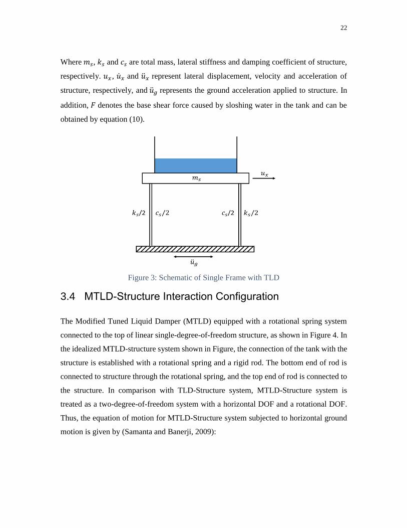
Where 𝑚𝑠, 𝑘𝑠 and 𝑐𝑠 are total mass, lateral stiffness and damping coefficient of structure,

respectively. 𝑢𝑥 , �̇�𝑥 and �̈�𝑥 represent lateral displacement, velocity and acceleration of

structure, respectively, and �̈�𝑔 represents the ground acceleration applied to structure. In

addition, 𝐹 denotes the base shear force caused by sloshing water in the tank and can be

obtained by equation (10).

Figure 3: Schematic of Single Frame with TLD

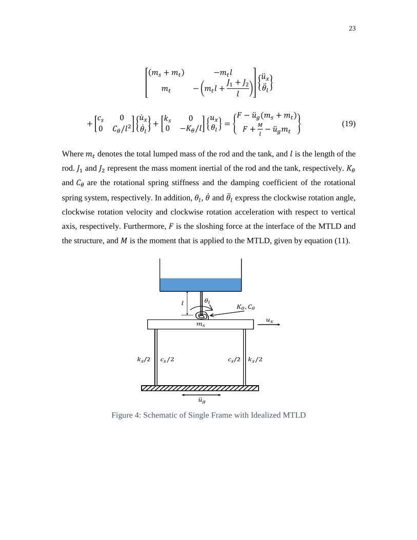
3.4 MTLD-Structure Interaction Configuration

The Modified Tuned Liquid Damper (MTLD) equipped with a rotational spring system

connected to the top of linear single-degree-of-freedom structure, as shown in Figure 4. In

the idealized MTLD-structure system shown in Figure, the connection of the tank with the

structure is established with a rotational spring and a rigid rod. The bottom end of rod is

connected to structure through the rotational spring, and the top end of rod is connected to

the structure. In comparison with TLD-Structure system, MTLD-Structure system is

treated as a two-degree-of-freedom system with a horizontal DOF and a rotational DOF.

Thus, the equation of motion for MTLD-Structure system subjected to horizontal ground

motion is given by (Samanta and Banerji, 2009):

23

[

(𝑚𝑠 + 𝑚𝑡) −𝑚𝑡𝑙

𝑚𝑡 − (𝑚𝑡𝑙 +𝐽1 + 𝐽2

𝑙)

] {�̈�𝑥

�̈�𝑙}

+ [𝑐𝑠 0

0 𝐶𝜃/𝑙2] {�̇�𝑥

�̇�𝑙} + [

𝑘𝑠 00 −𝐾𝜃/𝑙

] {𝑢𝑥

𝜃𝑙} = {

𝐹 − �̈�𝑔(𝑚𝑠 + 𝑚𝑡)

𝐹 +𝑀

𝑙− �̈�𝑔𝑚𝑡

} (19)

Where 𝑚𝑡 denotes the total lumped mass of the rod and the tank, and 𝑙 is the length of the

rod. 𝐽1 and 𝐽2 represent the mass moment inertial of the rod and the tank, respectively. 𝐾𝜃

and 𝐶𝜃 are the rotational spring stiffness and the damping coefficient of the rotational

spring system, respectively. In addition, 𝜃𝑙, �̇� and �̈�𝑙 express the clockwise rotation angle,

clockwise rotation velocity and clockwise rotation acceleration with respect to vertical

axis, respectively. Furthermore, 𝐹 is the sloshing force at the interface of the MTLD and

the structure, and 𝑀 is the moment that is applied to the MTLD, given by equation (11).

Figure 4: Schematic of Single Frame with Idealized MTLD

24

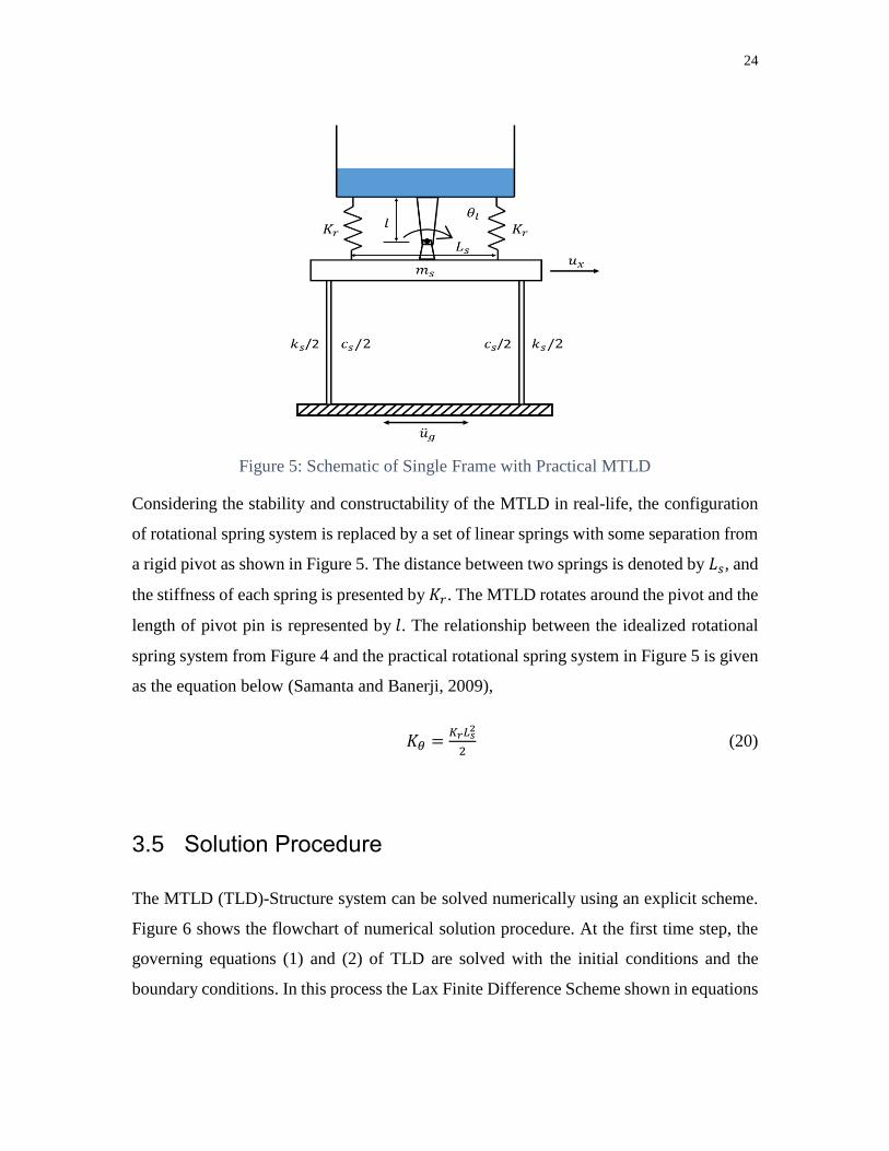
Figure 5: Schematic of Single Frame with Practical MTLD

Considering the stability and constructability of the MTLD in real-life, the configuration

of rotational spring system is replaced by a set of linear springs with some separation from

a rigid pivot as shown in Figure 5. The distance between two springs is denoted by 𝐿𝑠, and

the stiffness of each spring is presented by 𝐾𝑟. The MTLD rotates around the pivot and the

length of pivot pin is represented by 𝑙. The relationship between the idealized rotational

spring system from Figure 4 and the practical rotational spring system in Figure 5 is given

as the equation below (Samanta and Banerji, 2009),

𝐾𝜃 =𝐾𝑟𝐿𝑠

2

2 (20)

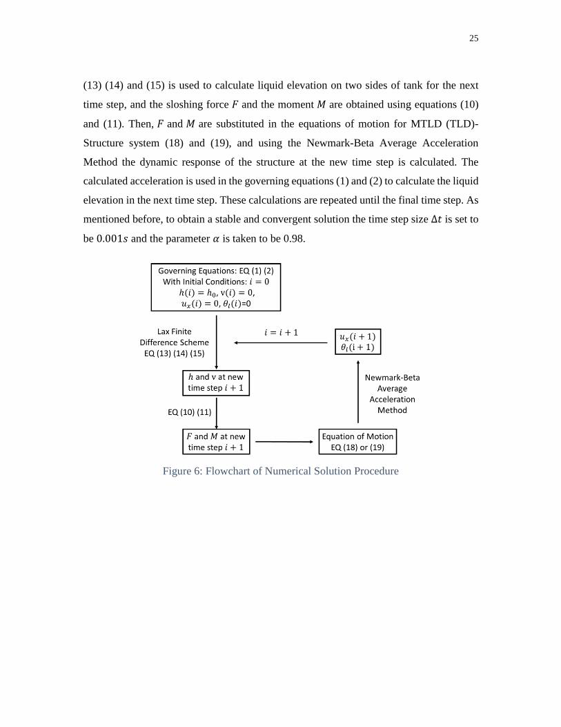
3.5 Solution Procedure

The MTLD (TLD)-Structure system can be solved numerically using an explicit scheme.

Figure 6 shows the flowchart of numerical solution procedure. At the first time step, the

governing equations (1) and (2) of TLD are solved with the initial conditions and the

boundary conditions. In this process the Lax Finite Difference Scheme shown in equations

25

(13) (14) and (15) is used to calculate liquid elevation on two sides of tank for the next

time step, and the sloshing force 𝐹 and the moment 𝑀 are obtained using equations (10)

and (11). Then, 𝐹 and 𝑀 are substituted in the equations of motion for MTLD (TLD)-

Structure system (18) and (19), and using the Newmark-Beta Average Acceleration

Method the dynamic response of the structure at the new time step is calculated. The

calculated acceleration is used in the governing equations (1) and (2) to calculate the liquid

elevation in the next time step. These calculations are repeated until the final time step. As

mentioned before, to obtain a stable and convergent solution the time step size ∆𝑡 is set to

be 0.001𝑠 and the parameter 𝛼 is taken to be 0.98.

Figure 6: Flowchart of Numerical Solution Procedure

26

Chapter 4

Numerical and Experimental Investigation

Results

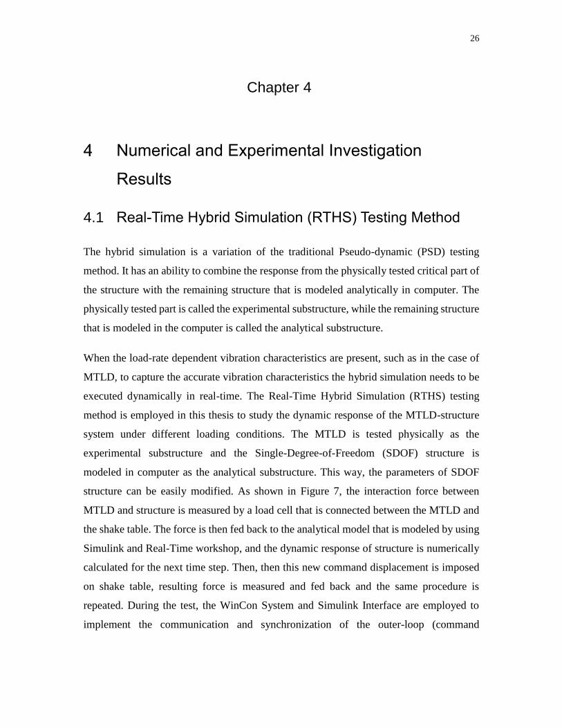
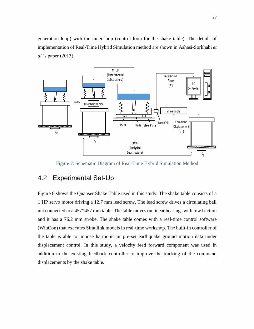
4.1 Real-Time Hybrid Simulation (RTHS) Testing Method

The hybrid simulation is a variation of the traditional Pseudo-dynamic (PSD) testing

method. It has an ability to combine the response from the physically tested critical part of

the structure with the remaining structure that is modeled analytically in computer. The

physically tested part is called the experimental substructure, while the remaining structure

that is modeled in the computer is called the analytical substructure.

When the load-rate dependent vibration characteristics are present, such as in the case of

MTLD, to capture the accurate vibration characteristics the hybrid simulation needs to be

executed dynamically in real-time. The Real-Time Hybrid Simulation (RTHS) testing

method is employed in this thesis to study the dynamic response of the MTLD-structure

system under different loading conditions. The MTLD is tested physically as the

experimental substructure and the Single-Degree-of-Freedom (SDOF) structure is

modeled in computer as the analytical substructure. This way, the parameters of SDOF

structure can be easily modified. As shown in Figure 7, the interaction force between

MTLD and structure is measured by a load cell that is connected between the MTLD and

the shake table. The force is then fed back to the analytical model that is modeled by using

Simulink and Real-Time workshop, and the dynamic response of structure is numerically

calculated for the next time step. Then, then this new command displacement is imposed

on shake table, resulting force is measured and fed back and the same procedure is

repeated. During the test, the WinCon System and Simulink Interface are employed to

implement the communication and synchronization of the outer-loop (command

27

generation loop) with the inner-loop (control loop for the shake table). The details of

implementation of Real-Time Hybrid Simulation method are shown in Ashasi-Sorkhabi et

al.’s paper (2013).

Figure 7: Schematic Diagram of Real-Time Hybrid Simulation Method

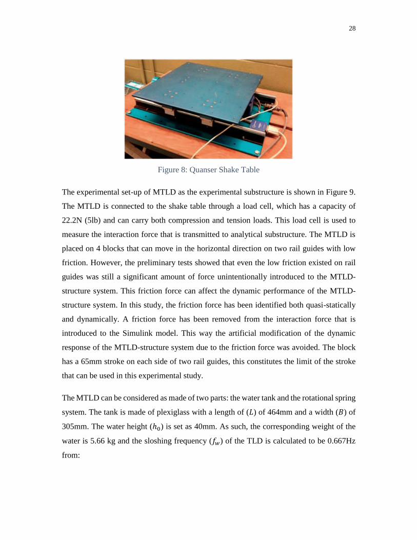
4.2 Experimental Set-Up

Figure 8 shows the Quanser Shake Table used in this study. The shake table consists of a

1 HP servo motor driving a 12.7 mm lead screw. The lead screw drives a circulating ball

nut connected to a 457*457 mm table. The table moves on linear bearings with low friction

and it has a 76.2 mm stroke. The shake table comes with a real-time control software

(WinCon) that executes Simulink models in real-time workshop. The built-in controller of

the table is able to impose harmonic or pre-set earthquake ground motion data under

displacement control. In this study, a velocity feed forward component was used in

addition to the existing feedback controller to improve the tracking of the command

displacements by the shake table.

28

Figure 8: Quanser Shake Table

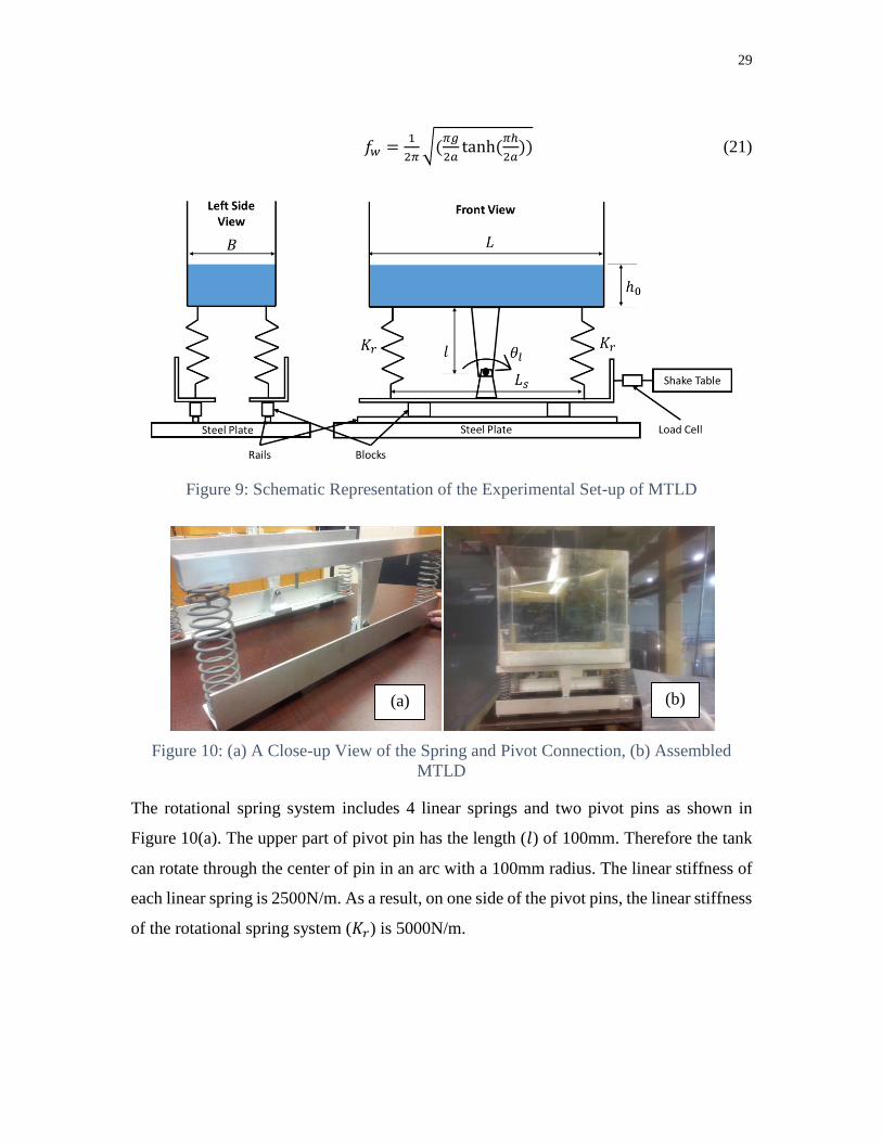
The experimental set-up of MTLD as the experimental substructure is shown in Figure 9.

The MTLD is connected to the shake table through a load cell, which has a capacity of

22.2N (5lb) and can carry both compression and tension loads. This load cell is used to

measure the interaction force that is transmitted to analytical substructure. The MTLD is

placed on 4 blocks that can move in the horizontal direction on two rail guides with low

friction. However, the preliminary tests showed that even the low friction existed on rail

guides was still a significant amount of force unintentionally introduced to the MTLD-

structure system. This friction force can affect the dynamic performance of the MTLD-

structure system. In this study, the friction force has been identified both quasi-statically

and dynamically. A friction force has been removed from the interaction force that is

introduced to the Simulink model. This way the artificial modification of the dynamic

response of the MTLD-structure system due to the friction force was avoided. The block

has a 65mm stroke on each side of two rail guides, this constitutes the limit of the stroke

that can be used in this experimental study.

The MTLD can be considered as made of two parts: the water tank and the rotational spring

system. The tank is made of plexiglass with a length of (𝐿) of 464mm and a width (𝐵) of

305mm. The water height (ℎ0) is set as 40mm. As such, the corresponding weight of the

water is 5.66 kg and the sloshing frequency (𝑓𝑤) of the TLD is calculated to be 0.667Hz

from:

29

𝑓𝑤 =1

2𝜋√(

𝜋𝑔

2𝑎tanh (

𝜋ℎ

2𝑎)) (21)

Figure 9: Schematic Representation of the Experimental Set-up of MTLD

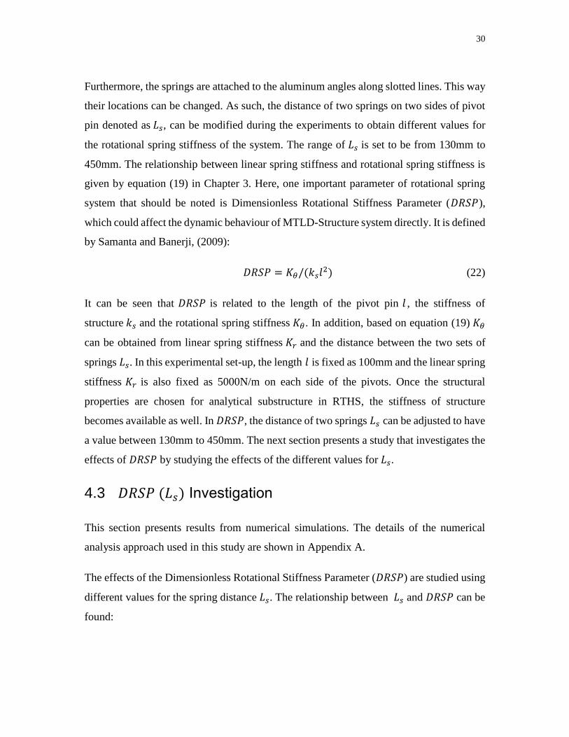
Figure 10: (a) A Close-up View of the Spring and Pivot Connection, (b) Assembled

MTLD

The rotational spring system includes 4 linear springs and two pivot pins as shown in

Figure 10(a). The upper part of pivot pin has the length (𝑙) of 100mm. Therefore the tank

can rotate through the center of pin in an arc with a 100mm radius. The linear stiffness of

each linear spring is 2500N/m. As a result, on one side of the pivot pins, the linear stiffness

of the rotational spring system (𝐾𝑟) is 5000N/m.

(a) (b)

30

Furthermore, the springs are attached to the aluminum angles along slotted lines. This way

their locations can be changed. As such, the distance of two springs on two sides of pivot

pin denoted as 𝐿𝑠, can be modified during the experiments to obtain different values for

the rotational spring stiffness of the system. The range of 𝐿𝑠 is set to be from 130mm to

450mm. The relationship between linear spring stiffness and rotational spring stiffness is

given by equation (19) in Chapter 3. Here, one important parameter of rotational spring

system that should be noted is Dimensionless Rotational Stiffness Parameter (𝐷𝑅𝑆𝑃),

which could affect the dynamic behaviour of MTLD-Structure system directly. It is defined

by Samanta and Banerji, (2009):

𝐷𝑅𝑆𝑃 = 𝐾𝜃/(𝑘𝑠𝑙2) (22)

It can be seen that 𝐷𝑅𝑆𝑃 is related to the length of the pivot pin 𝑙 , the stiffness of

structure 𝑘𝑠 and the rotational spring stiffness 𝐾𝜃. In addition, based on equation (19) 𝐾𝜃

can be obtained from linear spring stiffness 𝐾𝑟 and the distance between the two sets of

springs 𝐿𝑠. In this experimental set-up, the length 𝑙 is fixed as 100mm and the linear spring

stiffness 𝐾𝑟 is also fixed as 5000N/m on each side of the pivots. Once the structural

properties are chosen for analytical substructure in RTHS, the stiffness of structure

becomes available as well. In 𝐷𝑅𝑆𝑃, the distance of two springs 𝐿𝑠 can be adjusted to have

a value between 130mm to 450mm. The next section presents a study that investigates the

effects of 𝐷𝑅𝑆𝑃 by studying the effects of the different values for 𝐿𝑠.

4.3 𝐷𝑅𝑆𝑃 (𝐿𝑠) Investigation

This section presents results from numerical simulations. The details of the numerical

analysis approach used in this study are shown in Appendix A.

The effects of the Dimensionless Rotational Stiffness Parameter (𝐷𝑅𝑆𝑃) are studied using

different values for the spring distance 𝐿𝑠. The relationship between 𝐿𝑠 and 𝐷𝑅𝑆𝑃 can be

found:

31

𝐷𝑅𝑆𝑃 =𝐾𝑟𝐿𝑠

2

2𝑘𝑠𝑙2 (23)

In Equation 23, it can be seen that the value of 𝐷𝑅𝑆𝑃 can be adjusted by changing the

value of 𝐿𝑠 while other parameters remain constant as was done in this study. When the

rotational spring system is very stiff (i.e., a large value for 𝐿𝑠), since the resulting tank

rotations will be negligibly small, the MTLD can be treated as traditional TLD (i.e., as one,

that is rigidly connected to the structure). On the other hand, if the spring distance 𝐿𝑠 is

short, and the rotational spring stiffness is hence very small, the entire system may become

unstable. A previous research paper by Samanta and Banerji (2008) indicated the existence

of an optimum value for 𝐷𝑅𝑆𝑃, so that the Modified TLD can perform more effectively

than the traditional TLD. In this study, considering the properties of the experimental

setup, the effects of 𝐷𝑅𝑆𝑃 is first numerically studied by specifically considering different

values for the spring distance 𝐿𝑠.

The MTLD-Structure System is subjected to a series of sinusoidal excitations with a range

of excitation frequencies. The mass ratio (MR) between the MTLD mass (𝑚𝑤) to the

structural mass (𝑚𝑠) is kept to be 2%, and the damping ratio (𝜉) of structure remained as

1.2%. In addition, The MTLD-Structure System is investigated for three frequency ratios 𝛼

as 0.8, 1 and 1.2, which represent the ratio of the natural frequency of the structure 𝑓𝑠 to

the sloshing frequency 𝑓𝑤. The sloshing frequency 𝑓𝑤 is defined previously and remained

unchanged. Therefore, the structural stiffness 𝑘𝑠 should be adjusted to change the natural

frequency of structure 𝑓𝑠, to be able to obtain the afore-mentioned frequency ratios (i.e.,

different values for 𝛼 ). In the meantime, while changing the structural stiffness values, the

excitation amplitude is adjusted in a way to keep the same value of roof displacement for

the structure without MTLD. Furthermore, the frequency ratio 𝛽 between the excitation

frequency 𝑓 to the natural frequency of structure 𝑓𝑠 is considered to have several different

values in a range from 0.8 to 1.2. The properties of the MTLD-Structure system are listed

in Table 1.

32

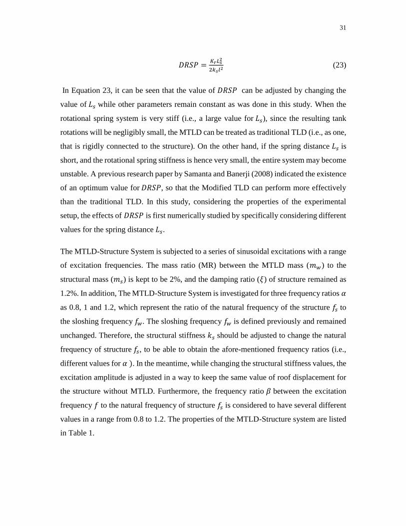
Table 1: The properties of MTLD-Structure System for DRSP Investigation

𝑚𝑤 (𝑘𝑔) 𝑚𝑠 (𝑘𝑔, 2%) 𝑓𝑤 (𝐻𝑧) 𝛼 𝑓𝑠 (𝐻𝑧) 𝑘𝑠 (𝑁/𝑚) 𝑐𝑠 (1.2%)

5.66

5.66

5.66

283.04

5.66

5.66

0.667

0.667

0.667

0.8 0.5336 3181.55 22.77

1 0.667 4971.18 28.47

1.2 0.8004 7158.49 34.16

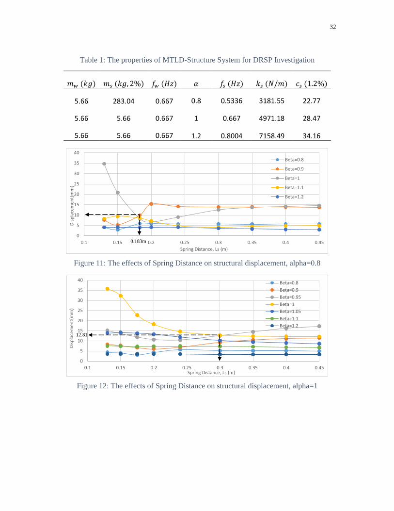
Figure 11: The effects of Spring Distance on structural displacement, alpha=0.8

Figure 12: The effects of Spring Distance on structural displacement, alpha=1

0

5

10

15

20

25

30

35

40

0.1 0.15 0.2 0.25 0.3 0.35 0.4 0.45

Dis

pla

cem

ent(

mm

)

Spring Distance, Ls (m)

Beta=0.8

Beta=0.9

Beta=1

Beta=1.1

Beta=1.2

0

5

10

15

20

25

30

35

40

0.1 0.15 0.2 0.25 0.3 0.35 0.4 0.45

Dis

pla

cem

ent(

mm

)

Spring Distance, Ls (m)

Beta=0.8

Beta=0.9

Beta=0.95

Beta=1

Beta=1.05

Beta=1.1

Beta=1.2

0.183m

12.81

33

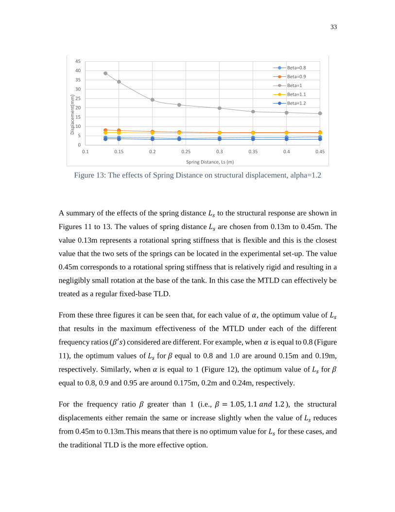
Figure 13: The effects of Spring Distance on structural displacement, alpha=1.2

A summary of the effects of the spring distance 𝐿𝑠 to the structural response are shown in

Figures 11 to 13. The values of spring distance 𝐿𝑠 are chosen from 0.13m to 0.45m. The

value 0.13m represents a rotational spring stiffness that is flexible and this is the closest

value that the two sets of the springs can be located in the experimental set-up. The value

0.45m corresponds to a rotational spring stiffness that is relatively rigid and resulting in a

negligibly small rotation at the base of the tank. In this case the MTLD can effectively be

treated as a regular fixed-base TLD.

From these three figures it can be seen that, for each value of 𝛼, the optimum value of 𝐿𝑠

that results in the maximum effectiveness of the MTLD under each of the different

frequency ratios (𝛽′𝑠) considered are different. For example, when 𝛼 is equal to 0.8 (Figure

11), the optimum values of 𝐿𝑠 for 𝛽 equal to 0.8 and 1.0 are around 0.15m and 0.19m,

respectively. Similarly, when 𝛼 is equal to 1 (Figure 12), the optimum value of 𝐿𝑠 for 𝛽

equal to 0.8, 0.9 and 0.95 are around 0.175m, 0.2m and 0.24m, respectively.

For the frequency ratio 𝛽 greater than 1 (i.e., 𝛽 = 1.05, 1.1 𝑎𝑛𝑑 1.2 ), the structural

displacements either remain the same or increase slightly when the value of 𝐿𝑠 reduces

from 0.45m to 0.13m.This means that there is no optimum value for 𝐿𝑠 for these cases, and

the traditional TLD is the more effective option.

0

5

10

15

20

25

30

35

40

45

0.1 0.15 0.2 0.25 0.3 0.35 0.4 0.45

Dis

pla

cem

ent(

mm

)

Spring Distance, Ls (m)

Beta=0.8

Beta=0.9

Beta=1

Beta=1.1

Beta=1.2

34

Figure 13 showed that for case when 𝛼 is equal to 1.2, the structural displacement response

for all range of frequency ratios 𝛽 are not reduced while the value of 𝐿𝑠 is reduced. In other

words, there is no optimum value of 𝐿𝑠 for al 𝛽. On the contrary the structural displacement

response will increase when the MTLD is employed in lieu of a fixed-base TLD.

Although the optimum value of 𝐿𝑠 is not unique for a range of frequency ratios 𝛽, in some

cases a specific value of 𝐿𝑠 can be determined such that with the use of this value of 𝐿𝑠 the

maximum value of the structural response can be kept below a certain value for the entire

range of frequency ratios 𝛽. This structural displacement value is also lower than that of

the structure equipped with the traditional TLD, indicating that a properly designed MTLD

is more efficient that the regular TLD at all frequency ratios 𝛽.

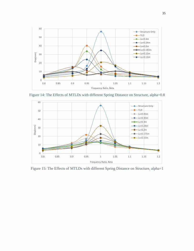
For the case when 𝛼 is equal to 0.8 as shown in Figures 11 and 14, when the value of 𝐿𝑠

is selected as 0.183m, the maximum displacement is less than 10mm, corresponding to a

value of 𝛽 equal to 0.9. At all other values of 𝛽 the maximum displacement values are

much less then 10mm for this 𝐿𝑠 value. If a different 𝐿𝑠 value is used, it can be seen that

the maximum structural displacement is no longer limited to a value of 10mm for all 𝛽

values, hence the structure can be observed experience larger displacements at some 𝛽

values. As such, for 𝛼 equal to 0.8, an 𝐿𝑠 value of 0.183m can be considered as the

optimum design value. Similarly from Figures 12 and 15, it can be concluded that for 𝛼

equal to 1 the optimum value of 𝐿𝑠 is 0.3m. In this case the maximum roof displacement

of the structure is less than 13 mm for all 𝛽 values. Unlike before, for 𝛼 equal to 1.2, it can

be seen from Figures 13 and 16 that over the entire range of 𝛽's the fixed-base TLD is

consistently more effective in reducing the displacements in comparison to MTLD. Thus,

there is no optimum value for 𝐿𝑠 and in the following sections of this study the case where

𝛼 equal to 1.2 is not further considered.

35

Figure 14: The Effects of MTLDs with different Spring Distance on Structure, alpha=0.8

Figure 15: The Effects of MTLDs with different Spring Distance on Structure, alpha=1

0

10

20

30

40

50

60

0.8 0.85 0.9 0.95 1 1.05 1.1 1.15 1.2

Dis

p(m

m)

Frequency Ratio, Beta

Structure Only

TLD

Ls=0.3m

Ls=0.24m

Ls=0.2m

Ls=0.183m

Ls=0.15m

Ls=0.13m

0

10

20

30

40

50

60

0.8 0.85 0.9 0.95 1 1.05 1.1 1.15 1.2

Dis

p(m

m)

Frequency Ratio, Beta

Structure Only

TLD

Ls=0.45m

Ls=0.35m

Ls=0.3m

Ls=0.24m

Ls=0.2m

Ls=0.175m

Ls=0.15m

36

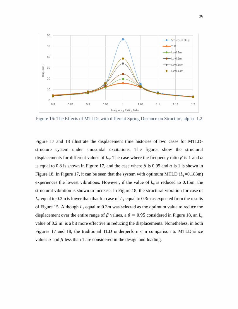
Figure 16: The Effects of MTLDs with different Spring Distance on Structure, alpha=1.2

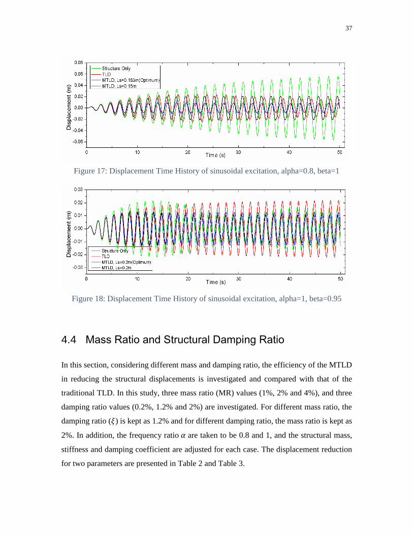
Figure 17 and 18 illustrate the displacement time histories of two cases for MTLD-

structure system under sinusoidal excitations. The figures show the structural

displacements for different values of 𝐿𝑠. The case where the frequency ratio 𝛽 is 1 and 𝛼

is equal to 0.8 is shown in Figure 17, and the case where 𝛽 is 0.95 and 𝛼 is 1 is shown in

Figure 18. In Figure 17, it can be seen that the system with optimum MTLD (𝐿𝑠=0.183m)

experiences the lowest vibrations. However, if the value of 𝐿𝑠 is reduced to 0.15m, the

structural vibration is shown to increase. In Figure 18, the structural vibration for case of

𝐿𝑠 equal to 0.2m is lower than that for case of 𝐿𝑠 equal to 0.3m as expected from the results

of Figure 15. Although 𝐿𝑠 equal to 0.3m was selected as the optimum value to reduce the

displacement over the entire range of 𝛽 values, a 𝛽 = 0.95 considered in Figure 18, an 𝐿𝑠

value of 0.2 m. is a bit more effective in reducing the displacements. Nonetheless, in both

Figures 17 and 18, the traditional TLD underperforms in comparison to MTLD since

values 𝛼 and 𝛽 less than 1 are considered in the design and loading.

0

10

20

30

40

50

60

0.8 0.85 0.9 0.95 1 1.05 1.1 1.15 1.2

Dis

p(m

m)

Frequency Ratio, Beta

Structure Only

TLD

Ls=0.3m

Ls=0.2m

Ls=0.15m

Ls=0.13m

37

Figure 17: Displacement Time History of sinusoidal excitation, alpha=0.8, beta=1

Figure 18: Displacement Time History of sinusoidal excitation, alpha=1, beta=0.95

4.4 Mass Ratio and Structural Damping Ratio

In this section, considering different mass and damping ratio, the efficiency of the MTLD

in reducing the structural displacements is investigated and compared with that of the

traditional TLD. In this study, three mass ratio (MR) values (1%, 2% and 4%), and three

damping ratio values (0.2%, 1.2% and 2%) are investigated. For different mass ratio, the

damping ratio (𝜉) is kept as 1.2% and for different damping ratio, the mass ratio is kept as

2%. In addition, the frequency ratio 𝛼 are taken to be 0.8 and 1, and the structural mass,

stiffness and damping coefficient are adjusted for each case. The displacement reduction

for two parameters are presented in Table 2 and Table 3.

38

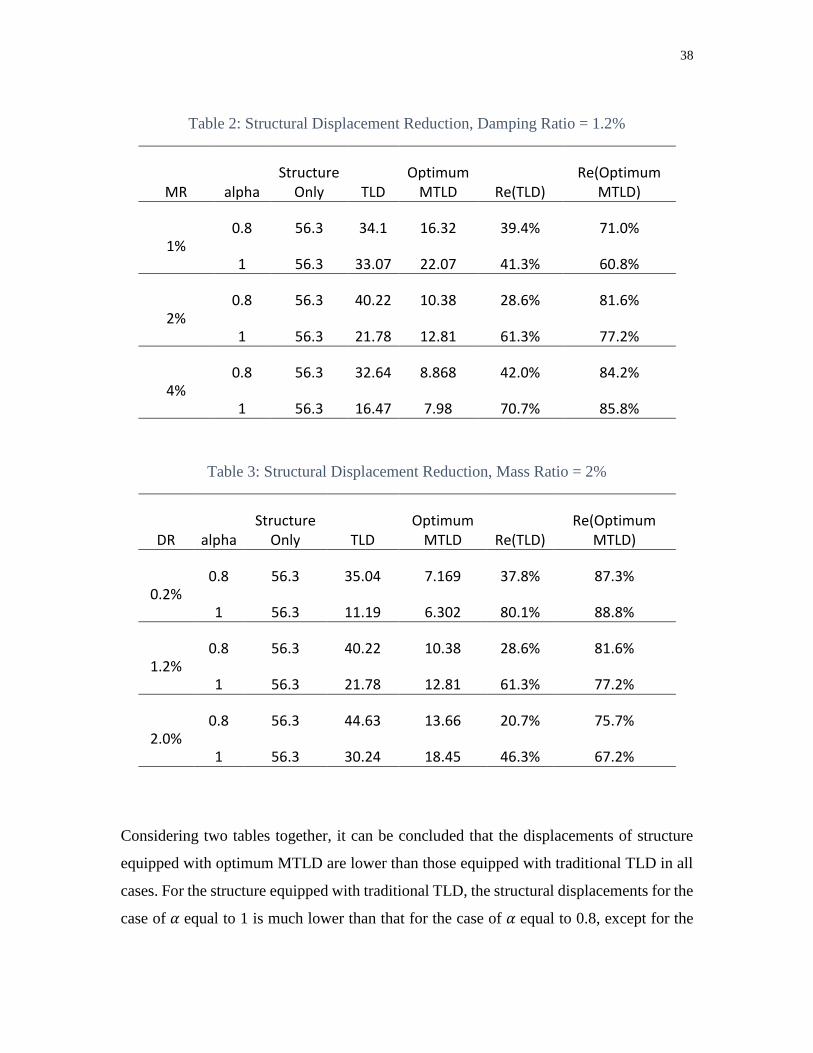
Table 2: Structural Displacement Reduction, Damping Ratio = 1.2%

MR alpha Structure

Only TLD Optimum

MTLD Re(TLD) Re(Optimum

MTLD)

1% 0.8 56.3 34.1 16.32 39.4% 71.0%

1 56.3 33.07 22.07 41.3% 60.8%

2% 0.8 56.3 40.22 10.38 28.6% 81.6%

1 56.3 21.78 12.81 61.3% 77.2%

4% 0.8 56.3 32.64 8.868 42.0% 84.2%

1 56.3 16.47 7.98 70.7% 85.8%

Table 3: Structural Displacement Reduction, Mass Ratio = 2%

DR alpha Structure

Only TLD Optimum

MTLD Re(TLD) Re(Optimum

MTLD)

0.2% 0.8 56.3 35.04 7.169 37.8% 87.3%

1 56.3 11.19 6.302 80.1% 88.8%

1.2% 0.8 56.3 40.22 10.38 28.6% 81.6%

1 56.3 21.78 12.81 61.3% 77.2%

2.0% 0.8 56.3 44.63 13.66 20.7% 75.7%

1 56.3 30.24 18.45 46.3% 67.2%

Considering two tables together, it can be concluded that the displacements of structure

equipped with optimum MTLD are lower than those equipped with traditional TLD in all

cases. For the structure equipped with traditional TLD, the structural displacements for the

case of 𝛼 equal to 1 is much lower than that for the case of 𝛼 equal to 0.8, except for the

39

case of MR equal to 1% and damping ratio equal to 2%. However, if the structure equipped

with optimum MTLD, the structural displacements for the case of 𝛼 equal to 1 is slightly

higher than those with 𝛼 equal to 0.8. This means that the optimum MTLD could provide

a higher reduction in displacements than the traditional TLD if is designed with a

frequency ratio 𝛼 that is less than 1.

From the Table 2, it can be seen that for both values of 𝛼, the displacement reduction of

structure equipped with optimum MTLD increases with the increasing mass ratio. This

indicates that an increase of mass ratio from 1% to 4% increases the effectiveness of

optimum MTLD.

In table 3, for both values of 𝛼, there is less reduction of the displacement of the structure

equipped with optimum MTLD as the damping ratio increases from 0.2% to 2%. The

results showed that the traditional TLD and optimum MTLD can perform more effectively

in a structure that has a low inherent damping ratio.

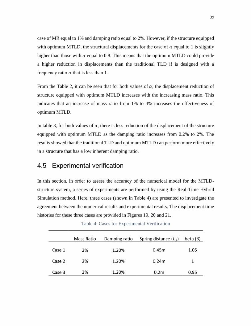
4.5 Experimental verification

In this section, in order to assess the accuracy of the numerical model for the MTLD-

structure system, a series of experiments are performed by using the Real-Time Hybrid

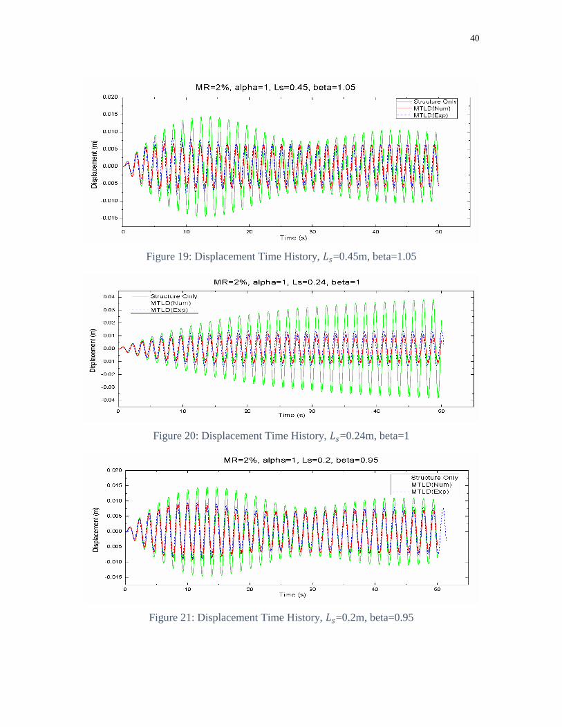
Simulation method. Here, three cases (shown in Table 4) are presented to investigate the

agreement between the numerical results and experimental results. The displacement time

histories for these three cases are provided in Figures 19, 20 and 21.

Table 4: Cases for Experimental Verification

Mass Ratio Damping ratio Spring distance (𝐿𝑠) beta (β)

Case 1 2%

2%

2%

1.20%

1.20%

1.20%

0.45m 1.05

Case 2 0.24m 1

Case 3 0.2m 0.95

40

Figure 19: Displacement Time History, 𝐿𝑠=0.45m, beta=1.05

Figure 20: Displacement Time History, 𝐿𝑠=0.24m, beta=1

Figure 21: Displacement Time History, 𝐿𝑠=0.2m, beta=0.95

41

In the first case (Figure 19), the oscillations in the experimental response is a little bit

higher than the numerical response in the beginning (around 10s) of the test. But after 15s,

the experimental result is the same as numerical results. In case 3 (Figure 21), the

amplitude of oscillations in the experiment is slightly bigger than the ones in the numerical

response both in the beginning and in the end; but still there is a good overall agreement

between the two responses. In case 2 (Figure 20), the discrepancy between the

experimental and numerical responses is more noticeable, however there is still an

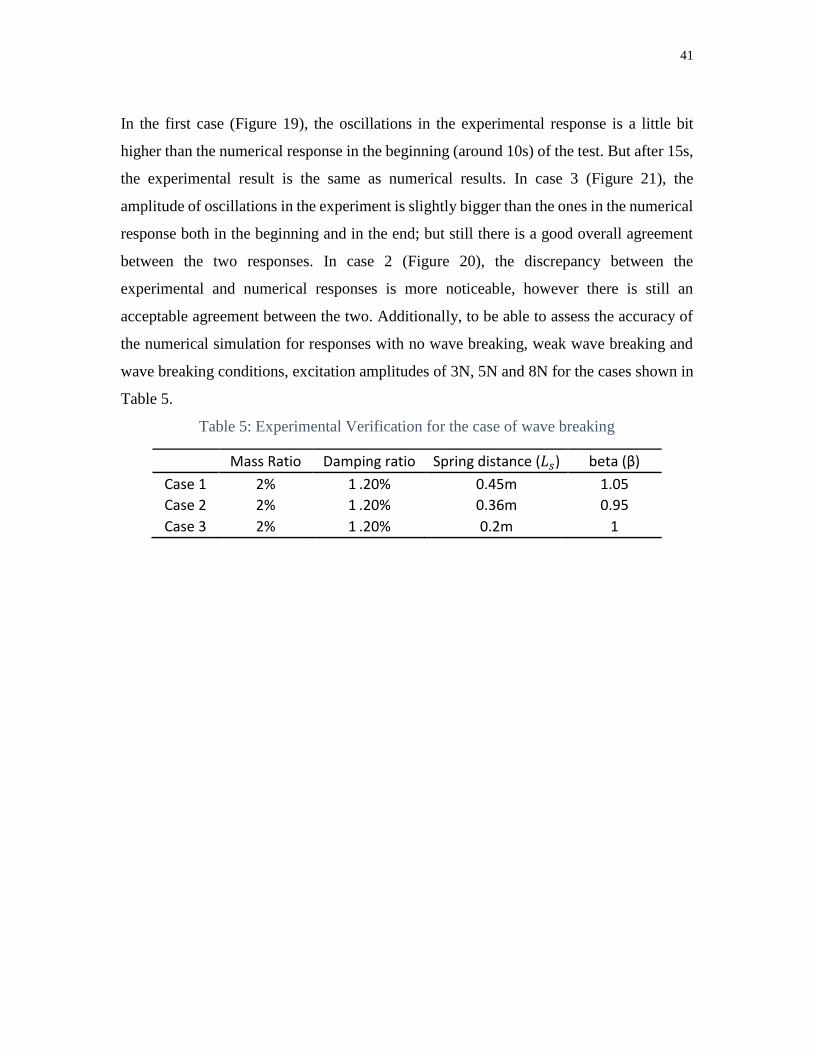
acceptable agreement between the two. Additionally, to be able to assess the accuracy of

the numerical simulation for responses with no wave breaking, weak wave breaking and

wave breaking conditions, excitation amplitudes of 3N, 5N and 8N for the cases shown in

Table 5.

Table 5: Experimental Verification for the case of wave breaking

Mass Ratio Damping ratio Spring distance (𝐿𝑠) beta (β)

Case 1 2% 1 .20% 0.45m 1.05

Case 2 2% 1 .20% 0.36m 0.95

Case 3 2% 1 .20% 0.2m 1

42

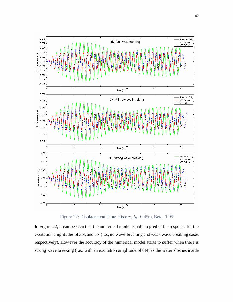
Figure 22: Displacement Time History, 𝐿𝑠=0.45m, Beta=1.05

In Figure 22, it can be seen that the numerical model is able to predict the response for the

excitation amplitudes of 3N, and 5N (i.e., no wave-breaking and weak wave breaking cases

respectively). However the accuracy of the numerical model starts to suffer when there is

strong wave breaking (i.e., with an excitation amplitude of 8N) as the water sloshes inside

43

the MTLD. It should be pointed out here that since 𝐿𝑠=0.45m is used, the cases in Figure

15 represents the limiting case where MTLD behaves as a fixed-base TLD.

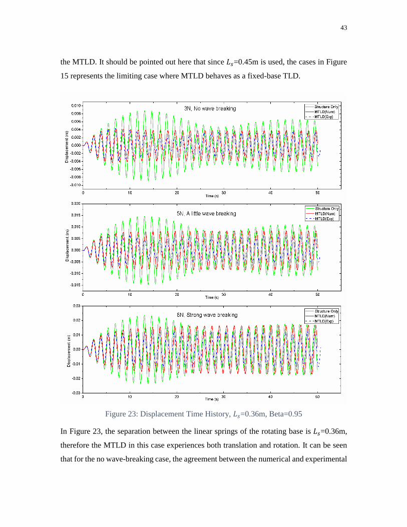
Figure 23: Displacement Time History, 𝐿𝑠=0.36m, Beta=0.95

In Figure 23, the separation between the linear springs of the rotating base is 𝐿𝑠=0.36m,

therefore the MTLD in this case experiences both translation and rotation. It can be seen

that for the no wave-breaking case, the agreement between the numerical and experimental

44

responses is good. However, it suffers as weak and strong wave breakings are observed in

the sloshing tank, under 5N, and 8N excitation amplitudes, respectively.

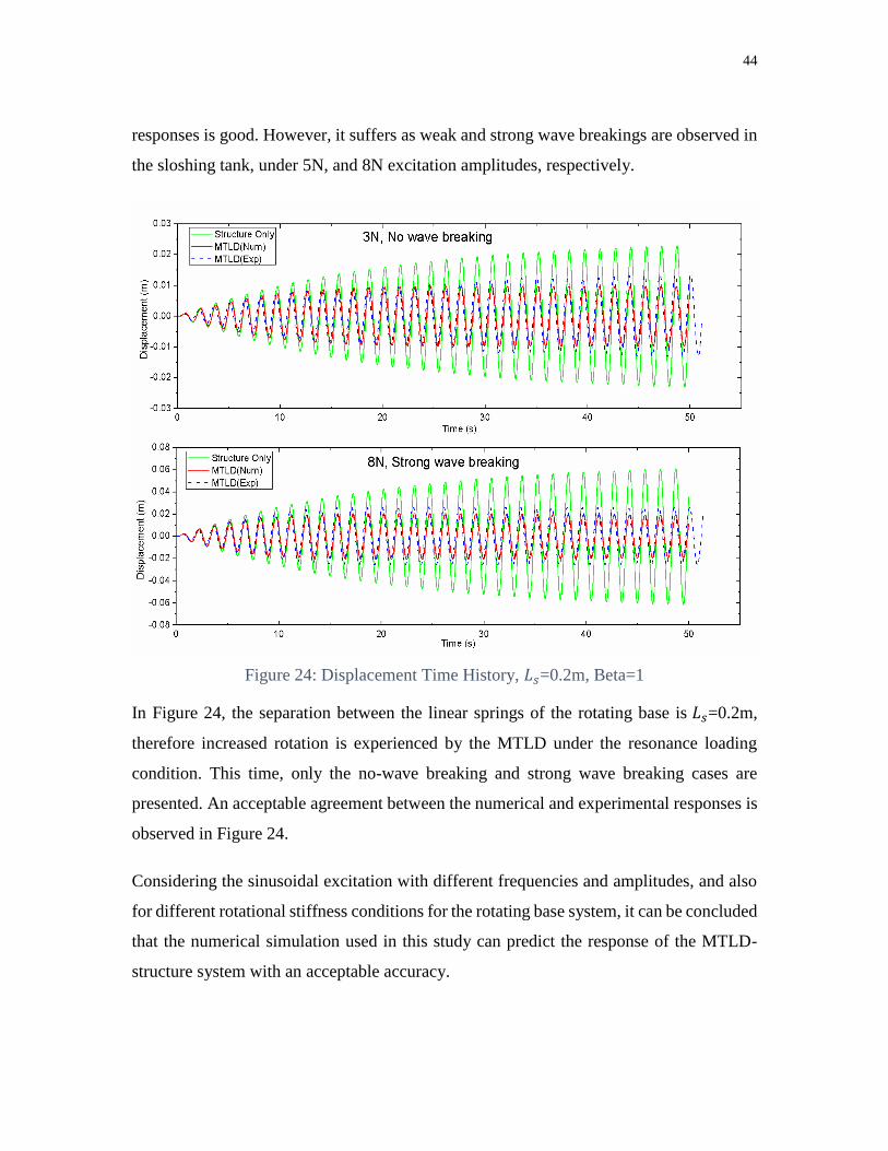
Figure 24: Displacement Time History, 𝐿𝑠=0.2m, Beta=1

In Figure 24, the separation between the linear springs of the rotating base is 𝐿𝑠=0.2m,

therefore increased rotation is experienced by the MTLD under the resonance loading

condition. This time, only the no-wave breaking and strong wave breaking cases are

presented. An acceptable agreement between the numerical and experimental responses is

observed in Figure 24.

Considering the sinusoidal excitation with different frequencies and amplitudes, and also

for different rotational stiffness conditions for the rotating base system, it can be concluded

that the numerical simulation used in this study can predict the response of the MTLD-

structure system with an acceptable accuracy.

45

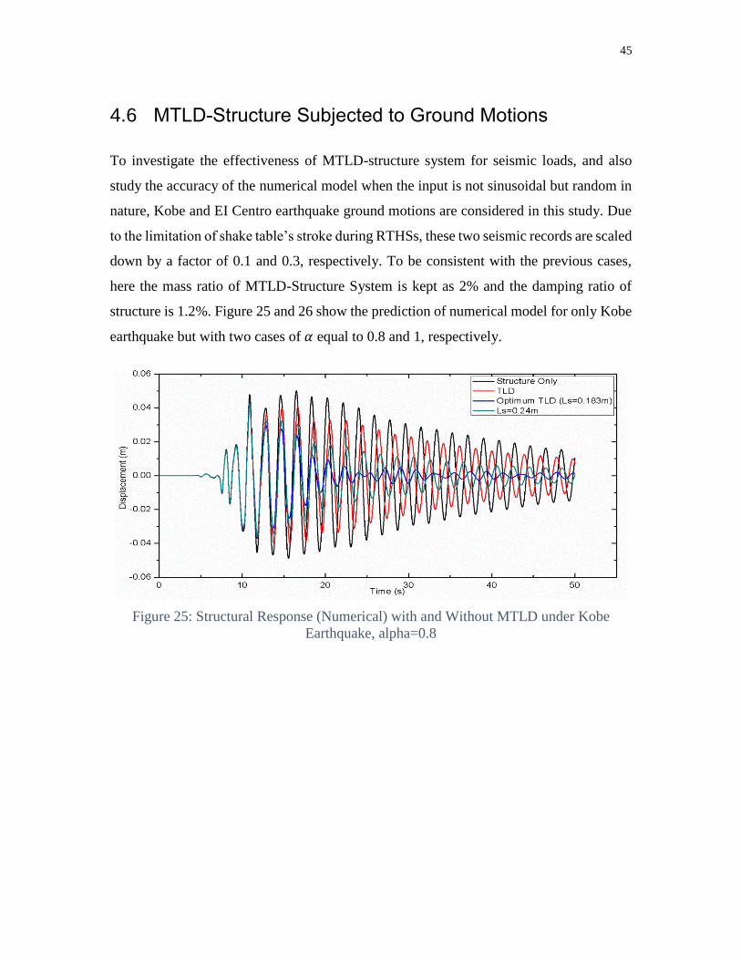
4.6 MTLD-Structure Subjected to Ground Motions

To investigate the effectiveness of MTLD-structure system for seismic loads, and also

study the accuracy of the numerical model when the input is not sinusoidal but random in

nature, Kobe and EI Centro earthquake ground motions are considered in this study. Due

to the limitation of shake table’s stroke during RTHSs, these two seismic records are scaled

down by a factor of 0.1 and 0.3, respectively. To be consistent with the previous cases,

here the mass ratio of MTLD-Structure System is kept as 2% and the damping ratio of

structure is 1.2%. Figure 25 and 26 show the prediction of numerical model for only Kobe

earthquake but with two cases of 𝛼 equal to 0.8 and 1, respectively.

Figure 25: Structural Response (Numerical) with and Without MTLD under Kobe

Earthquake, alpha=0.8

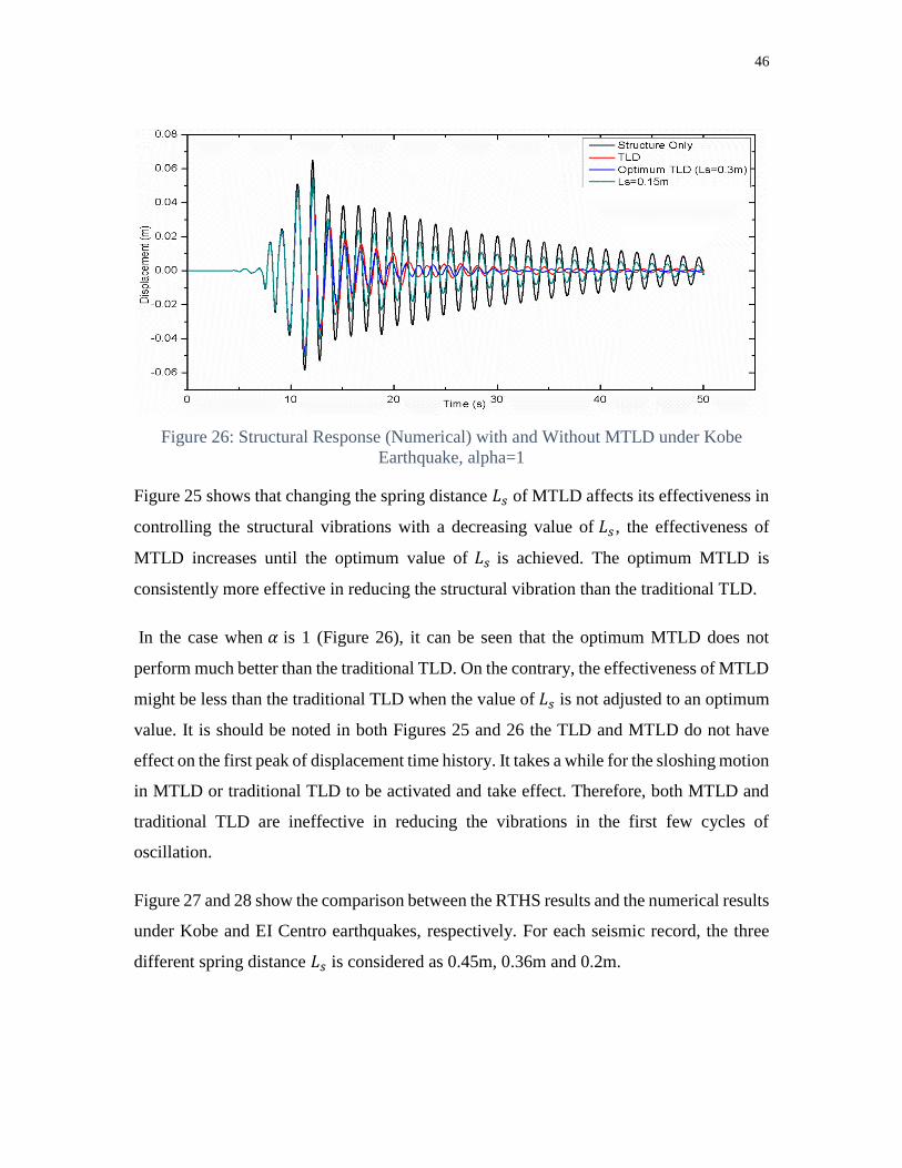
46

Figure 26: Structural Response (Numerical) with and Without MTLD under Kobe

Earthquake, alpha=1

Figure 25 shows that changing the spring distance 𝐿𝑠 of MTLD affects its effectiveness in

controlling the structural vibrations with a decreasing value of 𝐿𝑠 , the effectiveness of

MTLD increases until the optimum value of 𝐿𝑠 is achieved. The optimum MTLD is

consistently more effective in reducing the structural vibration than the traditional TLD.

In the case when 𝛼 is 1 (Figure 26), it can be seen that the optimum MTLD does not

perform much better than the traditional TLD. On the contrary, the effectiveness of MTLD

might be less than the traditional TLD when the value of 𝐿𝑠 is not adjusted to an optimum

value. It is should be noted in both Figures 25 and 26 the TLD and MTLD do not have

effect on the first peak of displacement time history. It takes a while for the sloshing motion

in MTLD or traditional TLD to be activated and take effect. Therefore, both MTLD and

traditional TLD are ineffective in reducing the vibrations in the first few cycles of

oscillation.

Figure 27 and 28 show the comparison between the RTHS results and the numerical results

under Kobe and EI Centro earthquakes, respectively. For each seismic record, the three

different spring distance 𝐿𝑠 is considered as 0.45m, 0.36m and 0.2m.

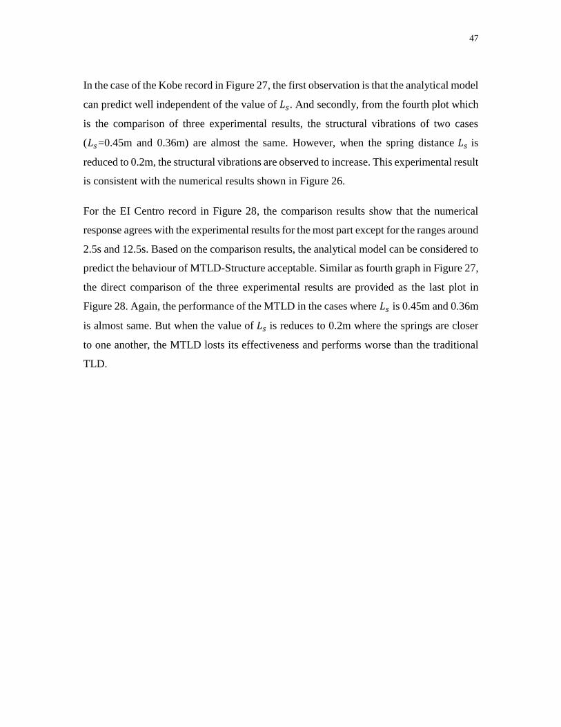
47

In the case of the Kobe record in Figure 27, the first observation is that the analytical model

can predict well independent of the value of 𝐿𝑠. And secondly, from the fourth plot which

is the comparison of three experimental results, the structural vibrations of two cases

(𝐿𝑠=0.45m and 0.36m) are almost the same. However, when the spring distance 𝐿𝑠 is

reduced to 0.2m, the structural vibrations are observed to increase. This experimental result

is consistent with the numerical results shown in Figure 26.

For the EI Centro record in Figure 28, the comparison results show that the numerical

response agrees with the experimental results for the most part except for the ranges around

2.5s and 12.5s. Based on the comparison results, the analytical model can be considered to

predict the behaviour of MTLD-Structure acceptable. Similar as fourth graph in Figure 27,

the direct comparison of the three experimental results are provided as the last plot in

Figure 28. Again, the performance of the MTLD in the cases where 𝐿𝑠 is 0.45m and 0.36m

is almost same. But when the value of 𝐿𝑠 is reduces to 0.2m where the springs are closer

to one another, the MTLD losts its effectiveness and performs worse than the traditional

TLD.

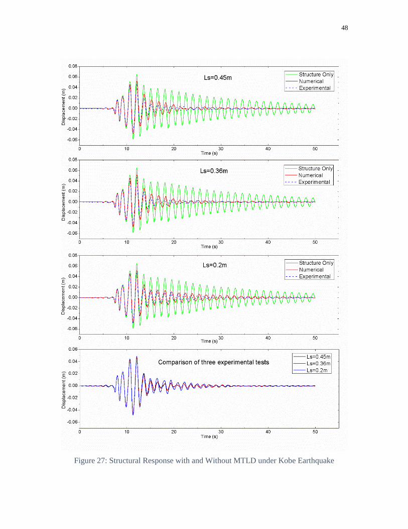
48

Figure 27: Structural Response with and Without MTLD under Kobe Earthquake

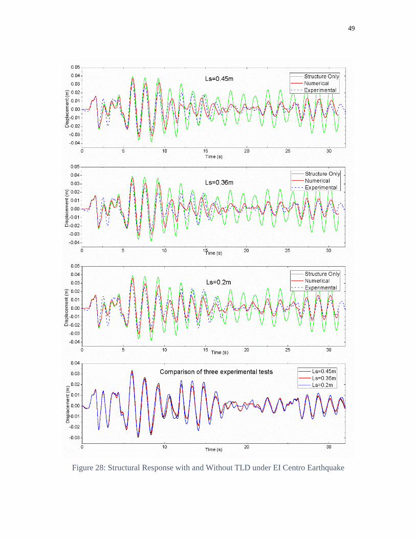
49

Figure 28: Structural Response with and Without TLD under EI Centro Earthquake

50

4.7 Preliminary Design Procedure

The results obtained from the numerical analyses and experiments using RTHS is used

here to propose a preliminary design procedure for MTLDs. The proposed design

procedure of MTLD considers a wide range of frequency ratio α (the ratio of the structural

natural frequency to the water sloshing frequency) and 𝛽 (the ratio of the excitation

frequency to the structural natural frequency). The details of preliminary design is

presented in Figure 29.

Design Procedure

1. Determine the structural vibration reduction percentage that is targeted.

2. If the desired reduction is less than around 60% traditional TLDs can be designed;

if more than 60%, proceed with the design of MTLDs.

3. Determine the properties of structure that need to be controlled, including the

structural mass, structural stiffness and structural damping ratio.

4. Use an α value of 0.8, and mass ratio in the range from 1% to 4%. For each mass

ratio, draw the displacement spectrum as done in Figures 14 and 15 of this chapter,

determine the optimum 𝐷𝑅𝑆𝑃 and mass ratio.

5. Using α, mass ratio and 𝐷𝑅𝑆𝑃 together with the structural properties, calculate the

tank dimensions, required water level and the connection details of the rotating

base.

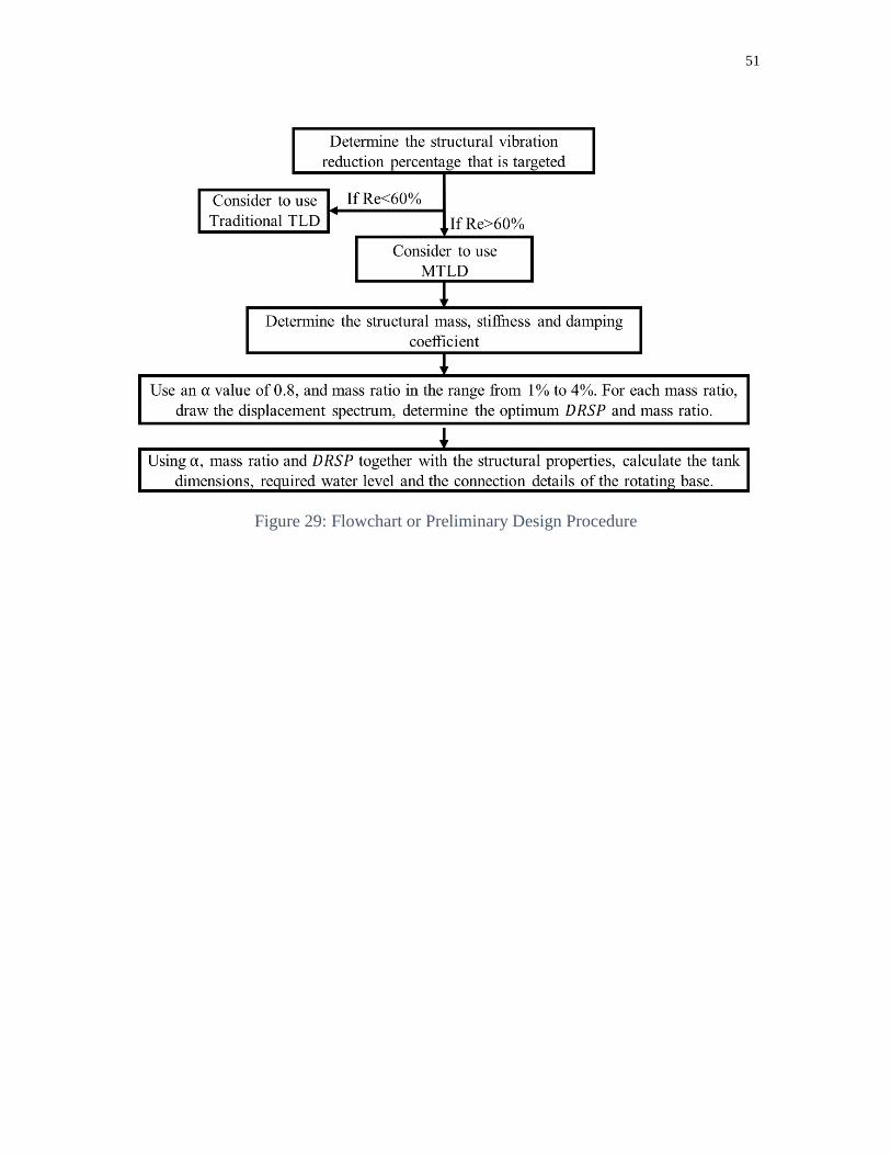
51

Figure 29: Flowchart or Preliminary Design Procedure

52

Chapter 5

Summary and Conclusion

In this study the Modified Tuned Liquid Damper (MTLD), where the Tuned Liquid

damper is attached to the structure with a rotating base to experience both translations and

rotations, is investigated numerically and experimentally. For the numerical study of the

effectiveness of MTLD-structure system in reducing the structural vibrations the numerical

model by Lu (2001) is used. For the experimental study, a state-of-the art testing method,

namely Real-time Hybrid Simulation (RTHS) is used, In these RTHSs a MTLD is tested

physically in the laboratory, while the structure is modeled in the computer; and the

response from these two are coupled in real-time.

Different parameters, such as mass ratio, frequency ratio 𝛼, damping ratio of structure and

also the excitation conditions, are considered in this study. The main conclusions regarding

the MTLD-structure response in comparison to the traditional TLD-structure response are

summarized below. Additionally a preliminary design procedure of MTLDs is proposed

in order to provide a starting point to the engineers in designing these devices.

𝐷𝑅𝑆𝑃 Investigation

The effects of the Dimensionless Rotational Stiffness Parameter (𝐷𝑅𝑆𝑃) that has already

been shown to be important in the MTLD-structure response, is considered in this study

by changing the distance between the linear springs 𝐿𝑠. It should be noted that the optimum

value of 𝐿𝑠 , where the MTLD exhibits the most effectiveness in reducing the vibrations,

is not unique under different excitation frequency (expressed by frequency ratio, 𝛽) for

each case of mass ratio and frequency ratio 𝛼. It was shown that an optimum value of 𝐿𝑠

is only possible for 𝛼 and 𝛽 values that are less than 1, where the properly designed MTLD

53

was shown to be more effective than the traditional TLD. In other cases however the

traditional TLDs were observed to be more efficient in controlling the vibrations.

Mass Ratio and Damping Ratio

By comparing the displacement reduction of MTLD-structure system between the cases of

different mass ratio, frequency ratio 𝛼 and damping ratio, it can be concluded that by using

the optimum value of 𝐿𝑠 a more effective MTLD can be designed by considering and 𝛼

value less than 1, a value of 0.8 is suggested in this study. Also, for different values of 𝛼,

the effectiveness of MTLD was shown to increase with an increasing mass ratio and with

a decreasing damping ratio.

Accuracy of Analytical model

The accuracy of the numerical simulation results were assessed using the experimental

results from real-time hybrid simulations. Sinusoidal excitations with different frequencies

and amplitudes were considered. The different amplitudes of the input excitation cause the

liquid in the sloshing to behave differently where no wave breaking, weak wave breaking

and strong wave breaking are observed. It was concluded that the numerical results

obtained in this study agree well with the experimental results for the no and weak wave

breaking cases. When strong wave breaking occurs the accuracy of the numerical

simulations suffer and their agreement with the experimentally obtained responses are still

acceptable.

The behaviour of the MTLD-structure system was also studied under two ground motions

both numerically and experimentally. The results show that the numerical model can

predict the structural vibration well under the Kobe earthquake but the accuracy suffers

under the EI Centro earthquake. However, it both cases the predictions of the numerical

simulations are acceptably accurate. By comparing the RTHS results with each other, it

was observed that even when it is optimally designed MTLD does not introduce much

additional efficiency in reducing the displacements when compared to the traditional TLD.

54

On the other hand, for MTLDs where the 𝐿𝑠 value was not optimally selected, the MTLD

response was worse than the traditional TLD response.

Future work

These further investigation and research areas are suggested for MTLDs:

Instead of a single-degree-of-freedom frame as done in this study, the interaction

of MTLDs with multi-degree-of-freedom structures should be studied. This will be

significant for practical applications.

Only two earthquake ground motions were used in this study. To be able to draw

general conclusions a more complete ground motion ensemble should be

considered.

55

References

Ashasi-Sorkhabi, A., Malekghasemi, H., & Mercan, O. (2013). Implementation and

verification of real-time hybrid simulation (RTHS) using a shake table for research

and education. Journal of Vibration and Control.

http://doi.org/10.1177/1077546313498616

Banerji, P., Murudi, M., Shah, A. H., & Popplewell, N. (2000). Tuned liquid dampers for

controlling earthquake response of structures. Earthquake Engineering and

Structural Dynamics, 29(5), 587–602. http://doi.org/10.1002/(SICI)1096-

9845(200005)29:5<587::AID-EQE926>3.0.CO;2-I

Banerji, P., Samanta, A., & Chavan, S. A. (2010). Earthquake vibration control of

structures using tuned liquid dampers: Experimental studies. International Journal

of Advance Structural Engineering, 2(2), 133–152.

Cassolato, M. R., Love, J. S., & Tait, M. J. (2011). Modelling of a tuned liquid damper

with inclined damping screens. Structural Control and Health Monitoring, 18, 674–

681. http://doi.org/10.1002/stc

Chang, C. C., & Gu, M. (1999). Suppression of vortex-excited vibration of tall buildings

using tuned liquid dampers. Journal of Wind Engineering and Industrial

Aerodynamics, 83(1-3), 225–237. http://doi.org/10.1016/S0167-6105(99)00074-4

Frandsen, J. B. (2005). Numerical predictions of tuned liquid tank structural systems.

Journal of Fluids and Structures, 20(3), 309–329.

http://doi.org/10.1016/j.jfluidstructs.2004.10.003

Fujino, Y., Sun, L., Pacheco, B. M., & Chaiseri, P. (1992). Tuned Liquid Damper (TLD)

For Suppressing Horizontal Motion of Structures. Journal of Engineering

Mechanics, 118(10), 2017–2030.

56

Gardarsson, S., Yeh, H., & Reed, D. (2001). BEHAVIOR OF SLOPED-BOTTOM

TUNED LIQUID DAMPERS. Journal of Engineering Mechanics, 127(3), 266–

271.

Ghaemmaghami, A., Kianoush, R., & Yuan, X.-X. (2013). Numerical Modeling of

Dynamic Behavior of Annular Tuned Liquid Dampers for Applications in Wind

Towers. Computer-Aided Civil and Infrastructure Engineering, 28(1), 38–51.

http://doi.org/10.1111/j.1467-8667.2012.00772.x

Halabian, A. M., & Torki, M. (2011). Numerical studies on the application of tuned

liquid dampers with screens to control seismic response of structures. The Structural

Design of Tall and Special Buildings, 20, 121–150. http://doi.org/10.1002/tal

ISHIBASHI, H., & Shinji, H. (1989). Nonlinear Response of Sloshing Based on the

shallow Water Wave Theory (2nd Report, Nonlinear Response in Rectangular

Tanks and Cylindrical Tanks). The Japan Society of Mechanical Engineers, (88-

0358), 663–670.

Kim, Y.-M., You, K.-P., & Cho, J.-E. (2006). The Vibration Performance Experiment of

Tuned Liquid Damper and Tuned Liquid Column Damper. Journal of Mechanical

Science and Technology, 20(6), 795–805.

KOH, C. G., MAHATMA, S., & WANG, C. M. (1994). THEORETICAL AND

EXPERIMENTAL STUDIES ON RECTANGULAR LIQUID DAMPERS UNDER

ARBITRARY EXCITATIONS. Earthquake Engineering and Structural Dynamics,

23, 17–31.

Koh, C. G., Mahatma, S., & Wang, C. M. (1995). Reduction of structural vibrations by

multiple-mode liquid dampers. Engineering Structures, 17(2), 122–128.

Lee, S. K., Park, E. C., Min, K. W., Lee, S. H., Chung, L., & Park, J. H. (2007). Real-

time hybrid shaking table testing method for the performance evaluation of a tuned

57

liquid damper controlling seismic response of building structures. Journal of Sound

and Vibration, 302(3), 596–612. http://doi.org/10.1016/j.jsv.2006.12.006

LI, H.-N., JIA, Y., & WANG, S.-Y. (2004). Theoretical and Experimental Studies on

Reduction for Multi-Modal Seismic Responses of High-Rise Structures by Tuned

Liquid Dampers. Journal of Vibration and Control, 10, 1041–1056.

Li, S. J., Li, G. Q., Tang, J., & Li, Q. S. (2002). Shallow rectangular TLD for structural

control implementation. Applied Acoustics, 63(10), 1125–1135.

http://doi.org/10.1016/S0003-682X(02)00022-1

LU, M. L., POPPLEWELL, N., SHAN, A. H., & CHAN, J. K. (2004). Nutation Damper

Undergoing a Coupled Motion. Journal of Vibration and Control, 10, 1313–1334.

http://doi.org/10.1177/1077546304042045

Malekghasemi, H. (2011). Experimental and Analytical Investigations of Rectangular

Tuned Liquid Dampers (TLDs).

Modi, V. J., & Akinturk, A. (2002). An efficient liquid sloshing damper for control of

wind-induced instabilities. Journal of Wind Engineering and Industrial

Aerodynamics, 90, 1907–1918. http://doi.org/10.1016/S0167-6105(02)00297-0

Modi, V. J., Akinturk, A., & Tse, W. (2003). A Family of Efficient Sloshing Liquid

Dampers for Suppression of Wind-Induced Instabilities. Journal of Vibration and

Control, 9, 361–386. http://doi.org/10.1177/107754603030773

Modi, V. J., & Munshi, S. R. (1998). An Efficient Liquid Sloshing Damper for vibration

control. Journal of Fluids and Structures, 12(fl980182), 1055–1071.

Modi, V. J., & Seto, M. L. (1998). Passive Control of Flow-Induced Oscillations Using

Rectangular Nutation Dampers. Journal of Vibration and Control, 4, 381–404.

http://doi.org/10.1177/107754639800400403

58

Modi, V. J., Welt, F., & Irani, M. B. (1990). On the suppression of vibrations using

nutation dampers. Journal of Wind Engineering and Industrial Aerodynamics, 33,

273–282. http://doi.org/10.1016/0167-6105(90)90043-C

Novo, T., Varum, H., Teixeira-Dias, F., Rodrigues, H., Silva, M. F., Costa, a. C., &

Guerreiro, L. (2014). Tuned liquid dampers simulation for earthquake response

control of buildings. Bulletin of Earthquake Engineering, 12(2), 1007–1024.

http://doi.org/10.1007/s10518-013-9528-2

Olson, D. E., & Reed, D. A. (2001). A nonlinear numerical model for sloped-bottom

tuned liquid dampers. Earthquake Engineering and Structural Dynamics, 30, 731–

743. http://doi.org/10.1002/eqe.34

Reed, D., Yu, J., Yeh, H., & Gardarsson, S. (1998). Investigation of Tuned liquid

dampers under large amplitude excitation. Journal of Engineering Mechanics,

124(4), 405–413. http://doi.org/10.1016/S0167-6105(98)00084-1

Samanta, A., & Banerji, P. (2008). Structural control using modified tuned liquid

dampers. In The 14th World Conference on Earthquake Engineering.

http://doi.org/10.1080/19373260903425410

Samanta, A., & Banerji, P. (2010). Structural vibration control using modified tuned

liquid dampers. The IES Journal Part A: Civil & Structural Engineering, 3(1), 14–

27. http://doi.org/10.1080/19373260903425410

Shad, H., Adnan, A. Bin, & Behbahani, H. P. (2013). Performance Evaluation of Tuned

Liquid Dampers on Response of a SDOF System Under Earthquake Excitation and

Harmonic Load. Research Journal of Applied Sciences, Engineering and

Technology, 6(16), 3018–3021.

Shimizu, T., & Hayama, S. (1989). Nonlinear Response of Sloshing Based on the

Shallow Water Wave Theory (1st Report, Derivation of Basic Equations and

59

Nonlinear Response in Rectangular Tanks). The Japan Society of Mechanical

Engineers, (86-0385), 357–363.

Siddique, M. R., Hamed, M. S., & Damatty, A. A. El. (2005). A nonlinear numerical

model for sloshing motion in tuned liquid dampers. International Journal of

Numerical Methods for Heat & Fluid Flow, 15(3), 306–324.

http://doi.org/10.1108/09615530510583900

Sun, L. (1991). Semi-Analytical Modelling of Tuned Liquid Damper(TLD) with

Emphasis on Damper of Liquid Sloshing.

Sun, L. M., Fujino, Y., Chaiseri, P., & Pacheco, B. M. (1995). The properties of tuned

liquid dampers using a TMD analogy. Earthquake Engineering and Structural

Dynamics, 24(7), 967–976. http://doi.org/10.1002/eqe.4290240704

Sun, L. M., Fujino, Y., & Koga, K. (1995). A MODEL OF TUNED LIQUID DAMPER

FOR SUPPRESSING PITCHING MOTIONS OF STRUCTURES. Earthquake

Engineering and Structural Dynamics, 24, 625–636.

Sun, L. M., Fujino, Y., Pacheco, B. M., & Chaiseri, P. (1992). Modelling of Tuned

Liquid Damper (TLD). Journal of Wind Engineering and Industrial Aerodynamics,

41-44, 1883–1894.

Sun, L. M., Fujino, Y., Pacheco, B. M., & Isobe, M. (1989). Nonlinear waves and

dynamic pressures in rectangular tuned liquid damper (TLD)-Simulation and

experimental verification. Structural engineering/Earthquake Engineering, 6(2),

81–92. http://doi.org/10.2208/jscej.1989.410_81

Tait, M. J. (2008). Modelling and preliminary design of a structure-TLD system.

Engineering Structures, 30(10), 2644–2655.

http://doi.org/10.1016/j.engstruct.2008.02.017

60

Tait, M. J., El Damatty, A. A., & Isyumov, N. (2005). An investigation of tuned liquid

dampers equipped with damping screens under 2D excitation. Earthquake

Engineering and Structural Dynamics, 34(7), 719–735.

http://doi.org/10.1002/eqe.452

Tait, M. J., El Damatty, A. A., Isyumov, N., & Siddique, M. R. (2005). Numerical flow

models to simulate tuned liquid dampers (TLD) with slat screens. Journal of Fluids

and Structures, 20(8), 1007–1023. http://doi.org/10.1016/j.jfluidstructs.2005.04.004

Tait, M. J., Isyumov, N., & El Damatty, A. A. (2007). Effectiveness of a 2D TLD and Its

Numerical Modeling. Journal of Structural Engineering, 133(2), 251–263.

http://doi.org/10.1061/(ASCE)0733-9445(2007)133:2(251)

Tamura, Y., Fujii, K., Ohtsuki, T., Wakahara, T., & Kohsaka, R. (1995). Effectiveness of

tuned liquid dampers under wind excitation. Engineering Structures, 17(9), 609–

621.

Tamura, Y., Kousaka, R., & Modi, V. J. (1992). Practical Application of Nutation

Damper for Suppressing Wind-Induced Vibrations of Airport Towers. Journal of

Wind Engineering and Industrial Aerodynamics, 41-44, 1919–1930.

Wakahara, T., Ohyama, T., & Fujii, K. (1992). Suppression of Wind-Induced Vibration

of a Tall Building using Tuned Liquid Damper. Journal of Wind Engineering and

Industrial Aerodynamics, (41-44), 1895–1906. http://doi.org/10.1016/0167-

6105(92)90615-H

Xin, Y., Chen, G., & Lou, M. (2009). Seismic response control with density-variable

tuned liquid dampers. Earthquake Engineering and Engineering Vibration, 8(4),

537–546. http://doi.org/10.1007/s11803-009-9111-7

Yu, J. K. (1997). Nonlinear Characteristics of Tuned Liquid Dampers. PhD. Thesis.

61

Yu, J., Wakahara, T., & Reed, D. A. (1999). A NON-LINEAR NUMERICAL MODEL

OF THE TUNED LIQUID DAMPER. Earthquake Engineering and Structural

Dynamics, 28, 671–686.

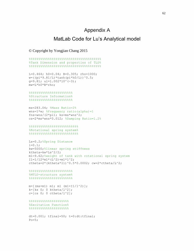
62

Appendix A

MatLab Code for Lu’s Analytical model

© Copyright by Yongjian Chang 2015 %%%%%%%%%%%%%%%%%%%%%%%%%%%%%%%%%%%%%% %Tank Dimension and properties of TLD% %%%%%%%%%%%%%%%%%%%%%%%%%%%%%%%%%%%%%%

L=0.464; h0=0.04; B=0.305; rho=1000; w=((pi*9.81/L)*tanh(pi*h0/L))^0.5; g=9.81; ul=1.002*10^(-3); mw=L*h0*B*rho;

%%%%%%%%%%%%%%%%%%%%%%% %Structure Information% %%%%%%%%%%%%%%%%%%%%%%%

ms=283.04; %Mass Ratio=2% wns=1*w; %Frequency ratio(alpha)=1 fns=wns/(2*pi); ks=ms*wns^2; cs=2*ms*wns*0.012; %Damping Ratio=1.2%

%%%%%%%%%%%%%%%%%%%%%%%%%% %Rotational spring system% %%%%%%%%%%%%%%%%%%%%%%%%%%

Ls=0.2;%Spring Distance l=0.1; kw=5000;%linear spring stiffness ktheta=kw*Ls^2/2; m1=9.62;%weight of tank with rotational spring system I1=1/12*m1*(L^2)+m1*l^2; ctheta=2*(ktheta*I1)^0.5*0.0002; cw=2*ctheta/L^2;

%%%%%%%%%%%%%%%%%%%%%%% %MTLD-structure system% %%%%%%%%%%%%%%%%%%%%%%%

m=[(ms+m1) m1; m1 (m1+I1/l^2)]; k=[ks 0; 0 ktheta/l^2]; c=[cs 0; 0 ctheta/l^2];

%%%%%%%%%%%%%%%%%%%%% %Excitation Function% %%%%%%%%%%%%%%%%%%%%%

dt=0.001; tfinal=50; t=0:dt:tfinal; Po=5;

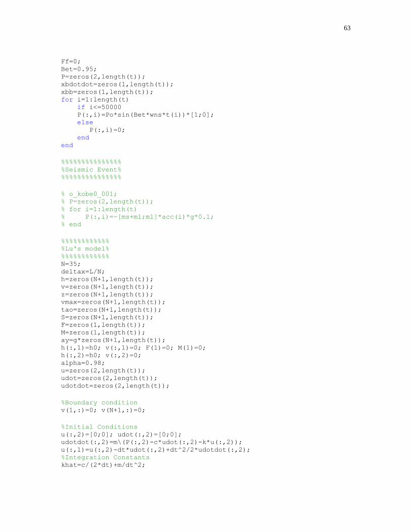
63

Ff=0; Bet=0.95; P=zeros(2,length(t)); xbdotdot=zeros(1,length(t)); xbb=zeros(1,length(t)); for i=1:length(t) if i<=50000 P(:,i)=Po*sin(Bet*wns*t(i))*[1;0]; else P(:,i)=0; end end

%%%%%%%%%%%%%%% %Seismic Event% %%%%%%%%%%%%%%%

% o_kobe0_001; % P=zeros(2,length(t)); % for i=1:length(t) % P(:,i)=-[ms+m1;m1]*acc(i)*g*0.1; % end

%%%%%%%%%%%% %Lu's model% %%%%%%%%%%%% N=35; deltax=L/N; h=zeros(N+1,length(t)); v=zeros(N+1,length(t)); z=zeros(N+1,length(t)); vmax=zeros(N+1,length(t)); tao=zeros(N+1,length(t)); S=zeros(N+1,length(t)); F=zeros(1,length(t)); M=zeros(1,length(t)); ay=g*zeros(N+1,length(t)); h(:,1)=h0; v(:,1)=0; F(1)=0; M(1)=0; h(:,2)=h0; v(:,2)=0; alpha=0.98; u=zeros(2,length(t)); udot=zeros(2,length(t)); udotdot=zeros(2,length(t));

%Boundary condition v(1,:)=0; v(N+1,:)=0;

%Initial Conditions u(:,2)=[0;0]; udot(:,2)=[0;0]; udotdot(:,2)=m\(P(:,2)-c*udot(:,2)-k*u(:,2)); u(:,1)=u(:,2)-dt*udot(:,2)+dt^2/2*udotdot(:,2); %Integration Constants khat=c/(2*dt)+m/dt^2;

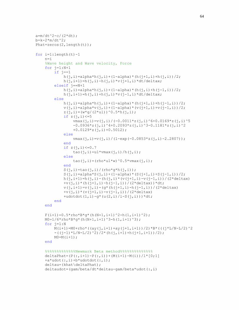
64

a=m/dt^2-c/(2*dt); b=k-2*m/dt^2; Phat=zeros(2,length(t));

for i=1:length(t)-1 n=i %Wave height and Wave velocity, Force for j=1:N+1 if j==1 h(j,i)=alpha*h(j,i)+(1-alpha)*(h(j+1,i)+h(j,i))/2; h(j,i+1)=h(j,i)-h(j,i)*v(j+1,i)*dt/deltax; elseif j==N+1 h(j,i)=alpha*h(j,i)+(1-alpha)*(h(j,i)+h(j-1,i))/2; h(j,i+1)=h(j,i)+h(j,i)*v(j-1,i)*dt/deltax; else h(j,i)=alpha*h(j,i)+(1-alpha)*(h(j+1,i)+h(j-1,i))/2; v(j,i)=alpha*v(j,i)+(1-alpha)*(v(j+1,i)+v(j-1,i))/2; z(j,i)=(w*g/(2*ul))^0.5*h(j,i); if z(j,i)<=5 vmax(j,i)=v(j,i)/(-0.0011*z(j,i)^6+0.0169*z(j,i)^5 -0.0936*z(j,i)^4+0.2093*z(j,i)^3-0.1181*z(j,i)^2 +0.0129*z(j,i)+0.5012); else vmax(j,i)=v(j,i)/(1-exp(-0.0853*z(j,i)-2.2807)); end if z(j,i)<=0.7 tao(j,i)=ul*vmax(j,i)/h(j,i); else tao(j,i)=(rho*ul*w)^0.5*vmax(j,i); end S(j,i)=tao(j,i)/(rho*g*h(j,i)); S(j,i)=alpha*S(j,i)+(1-alpha)*(S(j+1,i)+S(j-1,i))/2; h(j,i+1)=h(j,i)-(h(j,i)*(v(j+1,i)-v(j-1,i))/(2*deltax) +v(j,i)*(h(j+1,i)-h(j-1,i))/(2*deltax))*dt; v(j,i+1)=v(j,i)-(g*(h(j+1,i)-h(j-1,i))/(2*deltax) +v(j,i)*(v(j+1,i)-v(j-1,i))/(2*deltax) +udotdot(1,i)-g*(u(2,i)/l-S(j,i)))*dt; end end

F(i+1)=0.5*rho*B*g*(h(N+1,i+1)^2-h(1,i+1)^2); M0=1/6*rho*B*g*(h(N+1,i+1)^3-h(1,i+1)^3); for j=1:N M(i+1)=M0+rho*((ay(j,i+1)+ay(j+1,i+1))/2)*B*(((j*L/N-L/2)^2 -((j-1)*L/N-L/2)^2)/2*(h(j,i+1)+h(j+1,i+1))/2); M0=M(i+1); end

%%%%%%%%%%%%%Newmark Beta method%%%%%%%%%%%%%% deltaPhat=(P(:,i+1)-P(:,i))+(M(i+1)-M(i))/l*[0;1] +a*udot(:,i)+b*udotdot(:,i); deltau=(khat\deltaPhat); deltaudot=(gam/beta/dt*deltau-gam/beta*udot(:,i)

65

+dt*(1-gam/beta/2)*udotdot(:,i)); deltaudotdot=(1/beta/(dt^2))*deltau -udot(:,i)/beta/dt-udotdot(:,i)/2/beta; u(:,i+1)=u(:,i)+deltau; udot(:,i+1)=udot(:,i)+deltaudot; udotdot(:,i+1)=udotdot(:,i)+deltaudotdot; end

%%%%%%%%%%%%%%%%%%%%%%%%%%%%%%%%%%%%%%%%%%%%%%%%% %Calculating Structural Displacement Without MTLD% %Using Newmark-Beta Method%%%%%%%%%%%%%%%%%%%%%%% %%%%%%%%%%%%%%%%%%%%%%%%%%%%%%%%%%%%%%%%%%%%%%%%%

%Integration Constants kshat=ks+gam*cs/(beta*dt)+ms/(beta*dt^2); as=ms/(beta*dt)+gam*cs/beta; bs=ms/(2*beta)+dt*(gam/(2*beta)-1)*cs; %Initial Conditions uwo=zeros(1,length(t)); udotwo=zeros(1,length(t)); udotdotwo=zeros(1,length(t)); uwo(1)=0; udotwo(1)=0; udotdotwo(1)=(P(1,1)-cs*udotwo(1)-ks*uwo(1))/ms; for i=1:length(t)-1 deltaPhatwo=(P(1,i+1)-P(1,i))+as*udotwo(i)+bs*udotdotwo(i); deltauwo=deltaPhatwo/kshat; deltaudotwo=(gam/beta/dt*deltauwo-gam/beta*udotwo(i) +dt*(1-gam/beta/2)*udotdotwo(i)); deltaudotdotwo=(1/beta/(dt^2))*deltauwo -udotwo(i)/beta/dt-udotdotwo(i)/2/beta; uwo(i+1)=uwo(i)+deltauwo; udotwo(i+1)=udotwo(i)+deltaudotwo; udotdotwo(i+1)=udotdotwo(i)+deltaudotdotwo; end

66

Appendix B

List of Symbols

ℎ: Water height in sloshing motion

ℎ0: Water Height in steady state

𝐿: The length of water tank

𝐵: The width of water tank

𝑡: Time

v: Velocity of water sloshing

𝑥𝑏: Horizontal displacement of water tank

𝜃𝑏: Angle of rotation motion

𝑔: Gravity acceleration

𝑆: Slope of the energy grade line

𝜏𝑏: Liquid’s shear stress

𝜌: Density of liquid

𝜇: Dynamic viscosity of the liquid

𝜔: Excitation circular frequency

𝑣: Kinetic viscosity of the liquid

𝑧: Liquid’s dimensionless depth

𝐹: Interaction force caused by sloshing water

67

𝑀: Moment caused by sloshing water

𝑎𝑦: Vertical acceleration

𝑛: Division number

𝑚𝑠: Structural mass

𝑘𝑠: Structural stiffness

𝑐𝑠: Structural damping coefficient

𝑢𝑥: Structural displacement

�̇�𝑥: Structural velocity

�̈�𝑥: Structural acceleration

�̈�𝑔: Ground acceleration

𝐽: Mass moment inertial of the tank

𝜃𝑙: Rotational angle

�̇�𝑙: Rotational velocity

�̈�𝑙: Rotational acceleration

𝐾𝜃: Rotational spring stiffness

𝐾𝑟: Linear spring stiffness

𝐿𝑠: Linear spring distance

𝑓𝑤: Water sloshing frequency

𝑓𝑠: Natural frequency of structure

68

𝑓: Excitation frequency

𝛼: The ratio between sloshing frequency to structural natural frequency

𝛽: The ratio between excitation frequency to structural natural frequency

MR: Mass Ratio between water mass to structural mass

𝜉: Damping Ratio