Embed Size (px)
Citation preview

Helsinki University of Technology Doctoral Theses in Materials and Earth Sciences Laboratory of Mechanical Process Technology and Recycling Espoo 2006 TKK-ME-DT-4 AN INVESTIGATION OF THE EFFECT OF PHYSICAL AND CHEMICAL VARIABLES ON BUBBLE GENERATION AND COALESCENCE IN LABORATORY SCALE FLOTATION CELLS Rodrigo A. Grau Dissertation for the degree of Doctor of Science in Technology to be presented with due permission of the Department of Materials Science and Engineering for public examination and debate in Auditorium 1 at Helsinki University of Technology (Espoo, Finland) on the 9th
of January, 2006, at 12 noon. Helsinki University of Technology Department of Materials Science and Engineering Laboratory of Mechanical Process Technology and Recycling Teknillinen korkeakoulu Materiaalitekniikan osasto Mekaaninen prosessi- ja kierrätystekniikka
Helsinki University of Technology Laboratory of Mechanical Process Technology and Recycling P.O. Box 6200 FI-02015 TKK Available in pdf-format at http://lib.hut.fi/Diss/ © Rodrigo A. Grau Cover: Bubble generation, from left to right: (i) major fluid flows around the impeller fitted with two rotor/stator mechanisms, (ii) a close- up of the aerated cavity formed behind one of the blades of the OK rotor and (iii) air bubbles rising up through the viewing chamber in an aqueous solution of a frother. ISBN 951-22-7987-8 ISBN 951-22-7988-6(electronic) ISSN 1795-0074 HSE print Helsinki 2005

iii
ABSTRACT
A new technique for measuring bubble size in laboratory scale flotation cells was developed. A method of sampling and photographing bubbles from a flotation cell was combined with modern methods of image processing and analysis. The technique is capable of sizing accurately a large number of bubbles by exposing a stream of bubbles to a progressive scan camera
The technique was used to study the effect of several physical and chemical variables on bubbles size in laboratory scale flotation cells. Three mechanically agitated Outukumpu flotation cells were used in the tests, the size of the cells being 50 dm3, 70 dm3 and 265 dm3, respectively. The last mentioned was especially designed and constructed for this study. The cells were operated under batch conditions. The hydrodynamic conditions prevailing in the cells were modified mainly by altering the impeller speed and aeration conditions, as well as the frother concentration.
An extensive study of the effect of frother concentration on the bubbles generated in flotation cells was carried out. A series of common flotation frothers, DF-200, DF-250 and DF-1012, was chosen to test the effect of frothers on bubble coalescence and the bubble break-up process. The experimental tests revealed that bubble size strongly depends on frother concentration. With increasing frother concentration, the degree of bubble coalescence decreases, while at a particular frother concentration, known as the Critical Coalescence Concentration (CCC), bubble coalescence is totally hindered. The experimental results also indicate that frothers appear to affect the break-up process or bubble generation. While the DF-200 frother, characterized by much larger CCC values than DF-1012 and DF-250, has the ability to produce finer bubbles at concentrations exceeding the CCC value, the bubbles generated in the DF-1012 solutions at concentrations exceeding CCC are much larger.
The aeration rate has a profound impact on bubble generation; bubble size increases with an increase of the air flow rate entering the flotation cell. The aeration rate seems to determine to a large extent the size, shape and behaviour of the aerated cavities formed behind the blades of the rotor of the cell. These gassed cavities appear to control the mechanism of bubble generation in a flotation cell. The formation and behaviour of aerated cavities behind the Outokumpu rotor was examined using a high-speed camera.
While the maximum stable bubble diameter seems to characterize the bubble break-up process adequately, the Sauter mean bubble diameter and the number bubble mean diameter turned out not to be very sensitive to the changes in impeller speed. These two diameters are not always able to reveal adequately differences between bubble-size distributions.
Since bubble coalescence can be entirely prevented in the cell at frother concentrations exceeding the CCC values, it was possible to assess the impact of two commercial rotor/stator mechanisms on bubble generation. With the aid of a new sensor developed for measuring continuously local gas velocity, a series of tests was conducted to study how efficiently the incoming air is dispersed throughout the volume of the cell by the rotor/stator mechanism.
KEYWORDS: flotation; bubble size; gas dispersion; flotation frothers; critical coalescence concentration

iv
PREFACE
This thesis is dedicated to:
My friends,
My family,
And especially to my beloved wife Cecilia.
Espoo, January 2006, Rodrigo Grau

v
LIST OF PUBLICATIONS I-VI This work is based on the following papers (Appendices I-VI).
I. Grau, R.A., Heiskanen, K., 2002. Visual technique for measuring bubble size in flotation machines. Miner. Eng. 15 (7), 507-513.
II. Grau, R.A., Heiskanen, K., 2003. Gas dispersion measurements in a flotation cell. Miner. Eng. 16(11), 1081-1089.
III. Grau, R.A., Laskowski, J.S., Heiskanen, K., 2005. Effect of frothers on bubble size. Int. J. Miner. Process. 76(4), 225-233
IV. Grau, R.A., Heiskanen, K., 2005. Bubble size distribution in laboratory scale flotation cells. Miner. Eng. 18(12), 1164-1172.
V. Rudolphy, L., Grau, R.A., Heiskanen, K., 2005. On-line sensor for measuring superficial gas velocity in laboratory scale flotation machines. In: Jameson G. (Ed.), Proc. Centenary of Flotation Symposium. Austral. Inst. Min. Metall., Melbourne, pp. 573-580.
VI. Grau, R.A., Laskowski, J.S., 2005. Role of frothers in bubble generation and coalescence in a mechanical flotation cell. Accepted for publication in Can. J. Chem. Eng.
Note that in the text, each paper is referred to by the word Publication followed by its Roman numeral in bold. Author’s contribution In Publication I and II, the author planned and performed the experimental work and wrote the manuscript taking into account the comments of the co-author. Publication III is a joint paper between researchers at the Helsinki University of Technology and the University of British Columbia. The experimental program conducted at Helsinki University of Technology was planned by the author and was performed by, or under the supervision of, the author. The manuscript is the joint work of J.S Laskowski and R.A. Grau. In Publication IV, the author designed the experimental program; the experimental work was performed by, or under direct supervision of, the author. The manuscript was written by the author, taking into consideration the comments of the co-author. In Publication V, the author planned and designed the experimental work. The experimental work was performed by L. Rudolphy under the supervision of the author. The manuscript is the joint work of L. Rudolphy and R.A Grau. In publication VI, the author designed the experimental program. The experimental tests were performed by, or under direct supervision of, the author. The manuscript is the joint work of J.S Laskowski and R.A. Grau.

vi
The in-house software, which was used in combination with the commercial Matrox Inspector (image analysis software) and Microsoft Excel packages to capture and analyse the images of the bubbles, was developed solely by the author. The author was in charge of the design and construction of the 265 dm3 transparent Outokumpu cell, which was used in the experimental tests reported in Publications V and VI.

vii
CONTENTS
ABSTRACT ...............................................................................................................................iii PREFACE................................................................................................................................... iv LIST OF PUBLICATIONS I-VI................................................................................................. v CONTENTS ..............................................................................................................................vii LIST OF SYMBOLS AND ABBREVIATIONS.....................................................................viii 1 Introduction .................................................................................................................... 1
1.1 Frothers and bubble coalescence.................................................................................... 7 1.2 Objectives of this thesis.................................................................................................. 9 1.3 Thesis outline ................................................................................................................. 9
2 Bubble Size Analyser ................................................................................................... 11 2.1 The sampling technique ............................................................................................... 11 2.2 The software system..................................................................................................... 12 2.3 Image processing and blob analysis ............................................................................. 14
2.3.1 Mean bubble diameters......................................................................................... 20 2.3.2 Calibration of the images...................................................................................... 21
2.4 Validation study ........................................................................................................... 24 2.4.1 The correct threshold value .................................................................................. 27 2.4.2 Effect of compactness........................................................................................... 32 2.4.3 Number of bubbles sampled ................................................................................. 33
3 Experimental ................................................................................................................ 34 3.1 Laboratory-scale flotation cells .................................................................................... 34
3.1.1 Air flow rate.......................................................................................................... 34 3.1.2 Rotor/stator mechanisms ...................................................................................... 36 3.1.3 Impeller speed....................................................................................................... 36 3.1.4 Power measurements ............................................................................................ 37 3.1.5 Temperature of the liquid ..................................................................................... 37 3.1.6 Surface tension...................................................................................................... 38 3.1.7 Dynamic surface tension....................................................................................... 38 3.1.8 High-speed imaging system.................................................................................. 38
3.2 Bubble size measurements ........................................................................................... 39 4 Main Results and Discussion ....................................................................................... 41
4.1 Effect of frothers on bubble size .................................................................................. 41 4.1.1 Role of frothers in bubble coalescence and bubble generation ............................ 46
4.1.1.1 Critical Coalescence Concentration .................................................................48 4.1.1.2 Bubble coalescence ..........................................................................................50 4.1.1.3 Bubble break-up ...............................................................................................54 4.2 Effect of agitation on bubble generation ...................................................................... 57
4.2.1 Rotor/stator mechanisms ...................................................................................... 59 4.2.1.1 Mechanism of gas dispersion in the OK rotor..................................................63 4.3 Effect of air flow rate ................................................................................................... 67 4.4 Effect of a non-floatable solid ...................................................................................... 69
5 Summary and Final Remarks ....................................................................................... 70 6 Conclusions .................................................................................................................. 72 7 References .................................................................................................................... 74

LIST OF SYMBOLS AND ABBREVIATIONS
viii
LIST OF SYMBOLS AND ABBREVIATIONS
A Projected area of a single bubble, (mm2)
AB Surface area of a bubble, (m2)
Ac Cross-sectional area of the cell, (m2)
B Parameter which depends on the flow regime in the model of Yoon and Luttrell (1989)
BSA Bubble size analyser
C Concentration of particles in the suspension, in general in units of mass/volume
CCC Critical coalescence concentration, (mmol/dm3) or (ppm)
Cf Concentration of frother in the cell, (ppm) or (mol/dm3)
Cfo Lowest concentration of frother used in the tests, (ppm) or (mmol/dm3)
Comp Compactness of a bubble, dimensionless
CTP Correction factor for pressure and temperature
d10AM Linear (arithmetic) mean bubble diameter calculated using bubble projected-area diameters (uncorrected value), (mm)
d10spheres Mean size of glass spheres, (mm)
d10V or d10 Linear (arithmetic) mean bubble diameter calculated using bubble volume-equivalent diameters, diameter corrected for pressure and temperature, (mm)
d10VM Linear (arithmetic) mean bubble diameter calculated using bubble volume-equivalent diameters (uncorrected value), (mm)
d32 Sauter mean bubble diameter, (mm)
d32AM Sauter mean bubble diameter calculated using bubble projected-area

LIST OF SYMBOLS AND ABBREVIATIONS
ix
diameters (uncorrected value), (mm)
d32V or d32 Sauter mean bubble diameter calculated using bubble volume-equivalent diameters, diameter corrected for pressure and temperature, (mm)
d32VM Sauter mean bubble diameter calculated using bubble volume-equivalent diameters (uncorrected value), (mm)
d90 Bubble diameter such that 90% of the total gas volume is in bubbles of smaller diameter, (mm)
dAM Projected-area diameter measured at location M (uncorrected value), (mm)
db Bubble size, usually linear (arithmetic) mean bubble diameter, in general in units of (mm) or (µm)
dc Critical diameter of a stream tube, (mm)
DCell Diameter of the cell (tank diameter), (mm)
DI Rotor or impeller diameter, (mm)
dmax Maximum stable bubble diameter, (mm)
dp Particle diameter, in general in (µm)
dp50 Particle size, 50% passing size value, (µm)
dp80 Particle size, 80% passing size value , (µm)
dVM Bubble volume-equivalent diameter measured at location M (uncorrected value), (mm)
dV Bubble volume-equivalent diameter, in general in (mm) or (µm)
*10Vd Linear (arithmetic) mean bubble diameter calculated using bubble
volume-equivalent diameters measured manually, (mm)
*32Vd
Sauter mean bubble diameter calculated using bubble volume-equivalent diameters measured manually, (mm)
EK Collection efficiency
LIST OF SYMBOLS AND ABBREVIATIONS
x
f(x,y) Two-dimensional function which represents a greyscale image
F145 Feret diameter measured at an angle of 145°, (mm)
F90 Feret diameter measured at an angle of 90°, (mm)
Fmax Maximum Feret diameter, (mm)
Fmin Minimum Feret diameter, (mm)
G Number of grey levels in an image, in general G=28
g(x,y) Two-dimensional function which represents a binary image (after thresholding)
HM Distance between the point at which the bubbles are photographed and the froth /liquid interface, (m)
HUT Helsinki University of Technology
Jg Superficial gas velocity, (cm/s)
k Flotation rate constant calculated using concentrations in units of number of particles/volume, (1/s)
kc Flotation rate constant calculated using concentrations in units of mass/volume, (1/s)
L Path length in a suspension through which a single bubble rises, (m)
l Intensity value or greyscale value
M Number of rows in a matrix
n Exponent of the ratio particle diameter-to-bubble diameter in the models for calculating the probability of collision.
N Number of columns in a matrix
NC Number of particles collected by a single bubble
NI Impeller rotational speed, (rpm)

LIST OF SYMBOLS AND ABBREVIATIONS
xi
Np Number concentration of particles, (number of particles/dm3)
OK rotor Outokumpu rotor
OK-265 A 265 dm3 Outokumpu cell
OK-50 A 50 dm3 Outokumpu cell
OK-70 A 70 dm3 Outokumpu cell
OKFF Free-Flow rotor/stator design
OKMM Multi-Mix rotor/stator design
P Probability of particle collection
p A pixel
Pa Probability of adhesion between particles and bubbles
Pc Probability of collision between particles and bubbles
Pd Probability of detachment
Pdraw Power drawn by the cell mechanism, (kW)
Pdraw/V Power input per unit volume or specific power input, (kW/m3)
Pe Perimeter of the projected bubble, (mm)
Pf Parameter which represents the floatability of the mineral
Qg Volumetric air flow rate, in general (m3/min)
R The universal gas constant, 8.314 472 J/ (mol K)
Reb Bubble Reynolds number
Sb Bubble surface area flux, (m2/m2s)

LIST OF SYMBOLS AND ABBREVIATIONS
xii
t Flotation time, (s)
T Threshold intensity, greyscale value
TM Temperature in the viewing chamber, in (K)
Tm Temperature in kelvin, (K)
Tq Torque value, (N⋅m)
TS Impeller tip speed, (m/s)
UCT University of Cape Town
V Volume of liquid in the cell, (m3)
vb Bubble rise velocity, (m/s)
x Horizontal coordinate in a plane or image, a discrete quantity.
y Vertical coordinate in a plane or image, a discrete quantity.
Greek Symbols
Γ Surface excess per unit area, (mol/cm2)
α Constant depending on the particle-to-fluid density found in the empirical model given by Reay and Rattcliff (1973)
γ Surface tension, (mN/m)
β Dimensionless empirical exponent
ω Dimensionless empirical exponent
φ Dimensionless empirical constant
ρl Density of the liquid or continuous phase, (kg/m3)
ρp Density of a particle, (kg/m3)

LIST OF SYMBOLS AND ABBREVIATIONS
xiii
µl Viscosity of the liquid, in general (kg/m-s)


INRODUCTION
1
1 INTRODUCTION
Froth flotation is a versatile and extremely complex physico-chemical process that has been widely used in recovering valuable minerals. Flotation has also been applied to wastewater treatment, either for recovering valuable materials or for removing unwanted species. In flotation, hydrophobic particles are collected and transported by air bubbles from a liquid suspension to a froth phase, which has been stabilized with chemical agents known as frothers. It is from the froth that the collected particles are finally removed; hydrophilic particles remain in the liquid suspension uncollected. Hence, it is obvious that bubbles play a fundamental role in the flotation process and that the bubble size or the bubble size distribution has a critical effect on the collection process and transport of the material.
The role of bubbles in froth flotation can be studied by examining the effect of bubble size on the flotation rate constant. In general, the removal of particles in a flotation system has been modelled using a first-order kinetic model (Arbiter et al., 1962). In other words, the rate of flotation is constant with respect to the particle concentration. The rate of removal of particles from the suspension is given by Eq. (1), where C is the concentration of particles in the suspension in units of mass/volume and kc is the flotation rate constant.
Jameson et al. (1977) derived a simple model for the flotation rate constant in a small bubble column operated in a batch mode. The gas bubbles were generated at the bottom of a stagnant liquid contained in the vessel. They assumed that the rate of removal of particles in the vessel was a direct function of the number concentration of particles Np, as given in Eq. (2).
According to the model suggested by Jameson et al. (1977), the kinetic constant k is given by:
where Jg is the superficial gas velocity, db the bubble size and P the probability of collection. The collection process of hydrophobic particles has been described in terms of the probability of occurrence of a series of events. The probability of particle collection (P) by a bubble is given by (Sutherland, 1948; Yoon and Luttrell, 1989; Yoon, 2000):
CkdtdC
c−= (1)
pp kN
dtdN
−= (2)
PdJ
kb
g
23
= (3)
)1( dac PPPP −= (4)
INTRODUCTION
2
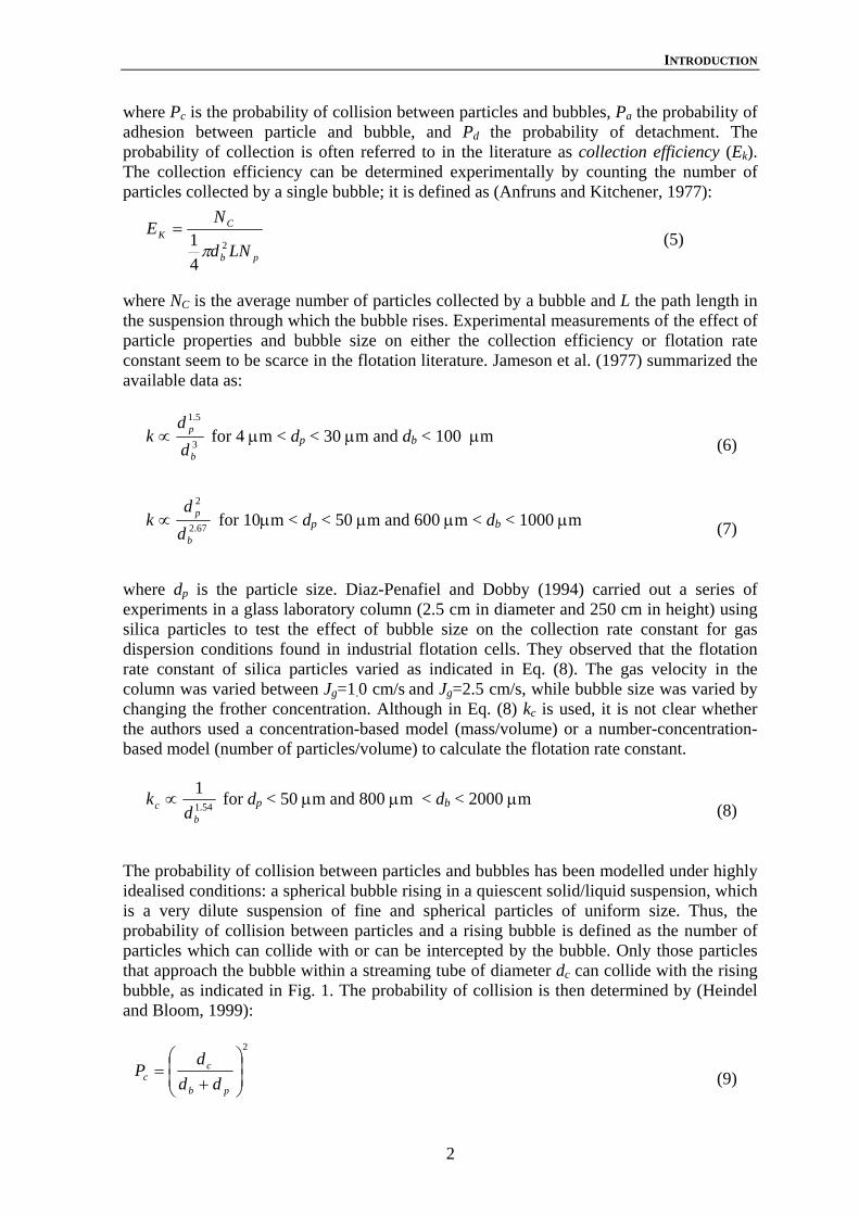
where Pc is the probability of collision between particles and bubbles, Pa the probability of adhesion between particle and bubble, and Pd the probability of detachment. The probability of collection is often referred to in the literature as collection efficiency (Ek). The collection efficiency can be determined experimentally by counting the number of particles collected by a single bubble; it is defined as (Anfruns and Kitchener, 1977):
where NC is the average number of particles collected by a bubble and L the path length in the suspension through which the bubble rises. Experimental measurements of the effect of particle properties and bubble size on either the collection efficiency or flotation rate constant seem to be scarce in the flotation literature. Jameson et al. (1977) summarized the available data as:
where dp is the particle size. Diaz-Penafiel and Dobby (1994) carried out a series of experiments in a glass laboratory column (2.5 cm in diameter and 250 cm in height) using silica particles to test the effect of bubble size on the collection rate constant for gas dispersion conditions found in industrial flotation cells. They observed that the flotation rate constant of silica particles varied as indicated in Eq. (8). The gas velocity in the column was varied between Jg=1.0 cm/s and Jg=2.5 cm/s, while bubble size was varied by changing the frother concentration. Although in Eq. (8) kc is used, it is not clear whether the authors used a concentration-based model (mass/volume) or a number-concentration-based model (number of particles/volume) to calculate the flotation rate constant.
The probability of collision between particles and bubbles has been modelled under highly idealised conditions: a spherical bubble rising in a quiescent solid/liquid suspension, which is a very dilute suspension of fine and spherical particles of uniform size. Thus, the probability of collision between particles and a rising bubble is defined as the number of particles which can collide with or can be intercepted by the bubble. Only those particles that approach the bubble within a streaming tube of diameter dc can collide with the rising bubble, as indicated in Fig. 1. The probability of collision is then determined by (Heindel and Bloom, 1999):
pb
CK
LNd
NE
2
41 π
= (5)
3
5.1
b
p
dd
k ∝ for 4 µm < dp < 30 µm and db < 100 µm (6)
67.2
2
b
p
dd
k ∝ for 10µm < dp < 50 µm and 600 µm < db < 1000 µm (7)
54.1
1
bc d
k ∝ for dp < 50 µm and 800 µm < db < 2000 µm (8)
2
⎟⎟⎠
⎞⎜⎜⎝
⎛
+=
pb
cc dd
dP (9)

INTRODUCTION
3
Fine particles will follow the fluid streamlines; it is usually assumed that the fluid streamlines come closest to the bubble at its equator. Hence a grazing trajectory is defined as the one that, at the bubble equator, passes within a distance of the particle radius from the bubble surface (Heindel and Bloom, 1999; Yoon and Mao, 1996). It can be inferred that only the particles located within the critical diameter dc at an infinite distance from the bubble can collide with it. The particles outside the critical diameter dc will sweep past the bubble. The dimension of dc depends on the nature of the flow regime. The determination of an expression for dc is largely dependent on the assumptions made about the dimensions of the bubble and particle.
Fig. 1. Particle colliding with a bubble at its equator. Reay and Ratcliff (1973) derived an expression for the probability of collision considering the case of a single particle interacting with a single bubble rising in contaminated water. They developed the model for small particles (<20 µm) and for fine bubbles (bubble diameter up to 100 µm) that were rising at their terminal velocity. Reay and Ratcliff (1973) obtained the following expression for the probability of collision:
n
b
pc d
dP ⎟⎟
⎠
⎞⎜⎜⎝
⎛= α (10)
(dc/2)
Particle with a diameter dp
Bubble
db
Fluid streamline

INTRODUCTION
4
where the constants α and n depend on the particle-to-fluid density ratio (ρp/ρl); a numerical solution gave an exponent n=2.05 for particles with ρp/ρl =2.5 and n=1.9 for ρp/ρf =1.0. Yoon and Luttrell (1989) derived a model for the probability of collision Pc, considering inertia-less particles (fine particles) that follow the streamlines formed around a rising bubble in a quiescent liquid. The generalized form of the model for Pc is given in Eq. (11), where the parameter B and the exponent n depend on the bubble Reynolds number. The model was developed for the intermediate range of bubble Reynolds numbers, and was validated using fine and very hydrophobic particles of coal. The bubble size ranged between 100 and 550 µm. The values of B and n for different flow regimes are shown in Table 1. The bubble Reynolds number is calculated as indicated in Eq. (12), where vb is the bubble rise velocity, ρl the density of the liquid and µl the viscosity of the liquid.
Table 1. Values of the parameters B and n of Eq. (11) (Yoon and Luttrell, 1989) Flow Regime B n Reynolds Stokes 3/2 2 Re →0
Intermediate 15
Re423 72.0
+ 2 0.2<Re<100
Potential 3 1 Re→∞ Note that, for completely hydrophobic particles, it is often assumed that Pa is equal to 1, whereas, for fine particles, Pd is equal to 0. According to the analysis of Yoon (2000) based on the model given in Eq. (11), it can be observed that, for highly hydrophobic fine particles and small bubbles (db < 100 µm), Pc varies as db
-2; therefore the flotation rate constant k varies as db
-3 (see Eq. (3)). However, for larger bubbles, the flotation rate constant becomes less dependent on the bubble size, and k varies only as db
-1.46. It is noteworthy that these observations are in good agreement with the empirical evidence as indicated in Eqs. (6) and (8). The empirical evidence summarized in Eqs. (6) to (8), and the models given in Eqs. (10) and (11), reveal a strong dependence of the flotation rate constant on the particle diameter; they also appear to indicate that, under quiescent conditions, the flotation of fine particles can be enhanced by the use of fine bubbles. Under turbulent conditions, as in mechanical cells, the study of the impact of bubble size on the flotation rate constant is complex, since it is difficult to isolate the different factors that could be affecting the flotation rate constant (Pc, Pa and Pd). In agitated flotation cells, the probability of collision between particles and bubbles is expected to increase with increasing agitation speed; however, the probability of detachment also becomes a
n
b
pc d
dBP ⎟⎟
⎠
⎞⎜⎜⎝
⎛= (11)
l
lbbdvµρ
=Re (12)

INTRODUCTION
5
dominant factor. Ahmed and Jameson (1985) concluded from batch flotation tests conducted in a small flotation cell that the flotation rate constant of fine particles is never as strongly dependent on the bubble size as in quiescent conditions, Eqs. (6) and (7). Using the data published by Ahmed and Jameson, it is possible to plot the flotation rate constant of fine quartz particles (25 µm < dp <40 µm) against bubble size, as shown in Fig. 2. As can be seen from Fig. 2, at a low agitation speed, the flotation rate constant seems to vary as db
-1.67, while, at a higher agitation intensity (300 rpm), the effect of the bubble size appears to become weaker (k varies as db
-1.46). Nevertheless, higher flotation rate constants are observed at bubble sizes below 200 µm. A further increment in agitation intensity appears to have a negative impact on the flotation rate constant. It must be emphasised that, when decreasing bubble size from 650 µm to 75 µm at low agitation speeds, a thirty-fold increase in the flotation rate constant is observed. It can be surmised that the rate of collision between bubbles and particles increases with increasing agitation intensity; however, intense agitation causes bubble-particle detachment, which appears to control the collection process. In the case of flotation of coarse particles, Tao (2004) deduced through a theoretical analysis that an increase in bubble size would produce an increase in the probability of detachment of coarse particles. Therefore, the flotation of coarse particles can be enhanced using finer bubbles. On the other hand, if the bubbles are too small, they will not have enough buoyancy to levitate coarse particles.
Fig. 2. Impact of bubble size on the flotation rate constant of fine quartz particles (Ahmed and Jameson, 1985).
Gorain et al. (1998, 1997, 1996, 1995b, 1995a) carried out an extensive investigation into the effect of impeller type, impeller speed, and air flow rate on gas dispersion conditions in an industrial scale flotation cell. A 3 m3 portable flotation cell was used for treating zinc cleaner feed. The feed solids concentration was around 35% and the particle size dp80 ranged from 20 to 25 µm. Gorain et al. (1998;1997) found that the collection zone rate constant is linearly correlated with Sb, the average bubble surface area flux in a flotation cell, as in:
0
0.01
0.02
0.03
0.04
0.05
0.06
0.07
0.08
0 100 200 300 400 500 600 700 800
Agitation 100 rpm
Agitation 300 rpm
Agitation 600 rpm67.15.41 −⋅= bdk
46.14.31 −⋅= bdk Flot
atio
n ra
te c
onst
ant k
(s-1
)
Bubble size db (um)

INTRODUCTION
6
where, Pf is a parameter that represents the mineral floatability and Sb the bubble surface area flux. Sb is calculated as indicated in Eq. (14), where Jg is the superficial gas velocity and d32 the Sauter mean bubble diameter. This model has been criticized by Heiskanen (2000) due to the fact that a very fine zinc rougher concentrate was used in the tests. Heiskanen also stated that the technique used for measuring bubble size produced a bias towards small bubbles. This produced an underestimation of the Sauter mean bubble diameter and therefore an overestimation of the bubble surface area flux in the cell. Nevertheless, the model indicates that the flotation rate constant in industrial flotation cells varies as db
-1, which is a weaker dependency than the one predicted using the interceptional
collision models.
Deglon et al. (1999) developed a kinetic model for agitated flotation cells, the attachment-detachment model. The model uses empirical equations developed for modelling the attachment and detachment of fine particles of quartz (95%-32 µm). The attachment-detachment model showed that the relationship between the collection zone rate constant and the bubble surface area flux is near linear only within a narrow range of Sb values (20 m2/m2s < Sb <60 m2/m2s), which corresponds to a zone of low agitation and therefore low detachment. It is also interesting to point out that Deglon and his co-workers found that, in batch flotation of fine particles of quartz (95% -32 µm), the flotation rate constant at low agitation varies as:
Eq. (15) shows a dependency on bubble size similar to the one observed in Fig. 2 at a low agitation speed. There seems to be clear indications that the use of fine bubbles may enhance the collection of particles in a flotation machine. The presence of fine bubbles combined with high air flow rates produces high air holdups (volume fraction of air in a flotation cell). In fact, high air holdups are the combination of fine bubbles in large numbers; in general, a high holdup is believed to have a positive effect on the collision rate. On the other hand, the use of fine bubbles could cause the loss of the pulp/froth interface in a flotation machine. Yianatos (2003) suggested that, at constant gas velocity, there exists a limiting condition, a minimum bubble size that will not cause interface loss. In a flotation cell, coarse particles attached to fine bubbles have a high probability of being dragged back to the zone of intensive agitation due to their low buoyancy or even to be discharged as tailings. However, the levitation of coarse particles might be strengthened by the formation of bubble clusters, which are held together by hydrophobic particles attached to two or more bubbles, as illustrated in Fig. 3. The presence of bubble clusters in laboratory scale cells as well as in industrial flotation cells has recently been reported by Ata and Jameson (2005).
bfc SPk = (13)
32
6dJ
S gb = (14)
6.1
2.0
b
pc d
dk ∝ (15)

INTRODUCTION
7
Fig. 3. Bubble clusters formed in the flotation of coarse particles of quartz (dp50=160 µm). Photograph taken with the bubble size equipment developed in this study (Grau and Heiskanen, 2003). Based on the above discussion, it might be expected in a mechanically agitated flotation cell that the probability or efficiency of collision between particles and bubbles governs the flotation of fine particles, whereas the mechanism controlling the flotation of coarse particles is detachment, and both mechanisms appear to be dependent on, among other factors, bubble size (Tao, 2004). It is likely that for each type of ore treated in a flotation machine there exists an optimum bubble size distribution that will produce the optimum recovery at the highest flotation rate (Jameson et al., 1977). The ability to control the generation of bubbles in order to produce an optimum size range in a flotation cell appears to be highly attractive, since it may enhance the efficiency of the flotation process by optimizing the collection of particles, i.e. by a better size-by-size flotation.
1.1 FROTHERS AND BUBBLE COALESCENCE
Frothers play a fundamental role in the flotation process. According to the Schulman-Leja penetration theory (Leja and Schulman, 1954; Leja, 1956/1957), frother molecules are preferentially adsorbed at the water/air interface, and their interaction with the collector molecules adsorbed on mineral particles in the moment of the particle-to-bubble attachment is a vital step in the attachment process. Because frothers adsorb at the air/liquid interface, they enhance gas dispersion into fine bubbles and stabilise the froth. The role of the froth in a flotation process is to act as a separating medium to segregate valuable mineral particles from gangue (Booth and Freyberger, 1962). Frother agents also dramatically enhance gas dispersion in flotation machines and reduce the size of the bubbles.
Laskowski and his co-workers (Cho and Laskowski, 2002a, 2002b; Laskowski et al. 2003; Laskowski 2003) have shown that frothers can be characterized using two parameters: the Critical Coalescence Concentration (CCC) and the Dynamic Foamabilty Index (DFI). They showed that frothers reduce bubble size by preventing bubbles from coalescing. As shown schematically in Fig. 4, with increasing frother concentration, the degree of bubble coalescence decreases and, at a particular frother concentration (CCC), the coalescence of
5 mm
INTRODUCTION
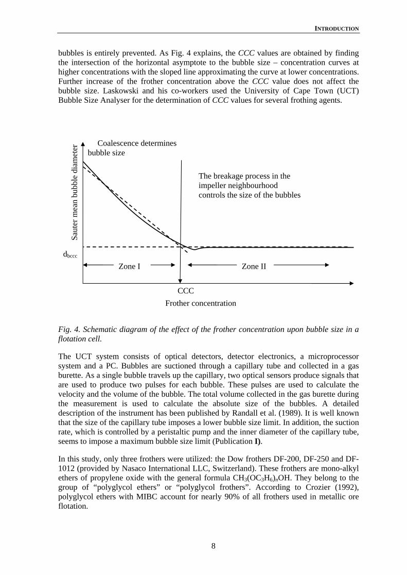
8
bubbles is entirely prevented. As Fig. 4 explains, the CCC values are obtained by finding the intersection of the horizontal asymptote to the bubble size – concentration curves at higher concentrations with the sloped line approximating the curve at lower concentrations. Further increase of the frother concentration above the CCC value does not affect the bubble size. Laskowski and his co-workers used the University of Cape Town (UCT) Bubble Size Analyser for the determination of CCC values for several frothing agents.
Fig. 4. Schematic diagram of the effect of the frother concentration upon bubble size in a flotation cell.
The UCT system consists of optical detectors, detector electronics, a microprocessor system and a PC. Bubbles are suctioned through a capillary tube and collected in a gas burette. As a single bubble travels up the capillary, two optical sensors produce signals that are used to produce two pulses for each bubble. These pulses are used to calculate the velocity and the volume of the bubble. The total volume collected in the gas burette during the measurement is used to calculate the absolute size of the bubbles. A detailed description of the instrument has been published by Randall et al. (1989). It is well known that the size of the capillary tube imposes a lower bubble size limit. In addition, the suction rate, which is controlled by a peristaltic pump and the inner diameter of the capillary tube, seems to impose a maximum bubble size limit (Publication I).
In this study, only three frothers were utilized: the Dow frothers DF-200, DF-250 and DF-1012 (provided by Nasaco International LLC, Switzerland). These frothers are mono-alkyl ethers of propylene oxide with the general formula CH3(OC3H6)nOH. They belong to the group of “polyglycol ethers” or “polyglycol frothers”. According to Crozier (1992), polyglycol ethers with MIBC account for nearly 90% of all frothers used in metallic ore flotation.
Saut
er m
ean
bubb
le d
iam
eter
dbccc
Frother concentration
Zone I Zone II
The breakage process in the impeller neighbourhood controls the size of the bubbles
Coalescence determines bubble size
CCC

INTRODUCTION
9
1.2 OBJECTIVES OF THIS THESIS The main objective of this thesis is to generate a better understanding of the mechanisms affecting and controlling bubble size, and thereby the phenomena of bubble coalescence and bubble generation in mechanically agitated flotation cells. This study deals with the effect of physical and chemical variables on bubble size in laboratory scale flotation cells. It also gives new insights into the phenomena of bubble generation and coalescence in this type of machine. The results of the study are expected to be directly relevant to the design and development of mechanically agitated flotation cells. The general aims of this study are:
(i) to develop techniques for measuring gas dispersion properties in laboratory scale flotation cells;
(ii) to validate the techniques and to determine the operating range of the new
sensors;
(iii) to study bubble generation in mechanical cells;
(iv) to study how efficiently the air is dispersed by different cell mechanisms (rotor/stator mechanism);
(v) to characterize different rotor/stator mechanisms in terms of bubble size;
(vi) to identify the operating conditions under which the bubble size characterizes
the performance of the rotor/stator mechanism;
(vii) to provide measurement data for validating numerical models of flotation cells.
1.3 THESIS OUTLINE
This thesis comprises six publications that deal with different aspects of gas dispersion conditions in laboratory scale flotation cells.
Publication I and II
The first steps towards the developments of a technique for measuring bubble size are reported in Publications I and II. Publication II also introduces a technique for measuring local gas velocity in an on-line manner and a simple method for measuring local gas holdup.
In Publication I, bubble sizes measured in a laboratory scale cell using the new technique and the UCT bubble size analyser are compared. The results reveal interesting aspects of the operation of the bubble sizing methods like, for example, the operating range.
INTRODUCTION
10
Publication III and VI
A comprehensive study of the role of frothers in bubble generation and bubble coalescence is presented in Publications III and VI.
In Publication III, the validity of the Critical Coalescence Concentrations values of a family of Dow frothers (mono-alkyl ethers of propylene oxide) is studied using the new technique for measuring bubble size; the CCC values obtained are compared to the values obtained by Laskowski et al. (2003) using the UCT technique. The experimental work revealed that frothers seem to also affect bubble generation. In Publication VI, the role of frothers in bubble coalescence and bubble generation is further studied.
Publication IV
The effect of several physical variables such as air flow rate, impeller speed, power consumption and type of rotor/stator on the generation of bubbles is studied and reported in Publication IV
Publication V
The validation and an analysis of the advantages and drawbacks of the sensor developed for measuring local gas velocity are presented in Publication V. The new sensor was used to study the impact of several factors, such as air flow rate, impeller speed and frother dosage on gas dispersion conditions prevailing in a flotation cell.
Thesis
In this thesis, a compendium of the main results of the research work is presented. A complete overview of the technique developed for measuring bubble size is also given here, as well as a description of the methods used in the validation work. The compendium also comprises unpublished results that complement the studies reported in Publications I to VI.
Publications I to VI are included in Sections I to VI.

HUT BUBBLE SIZE ANALYSER
11
2 BUBBLE SIZE ANALYSER
A novel technique for measuring bubble size in laboratory flotation cells was first reported in Publication I. The technique combines bubble visualization methods; the bubbles are exposed to a monochrome camera and subjected to image analysis. The technique for measuring bubble size has been modified throughout the course of the research work (Publication II, III, IV and VI). For instance, several modifications were made to the sampling technique and to the methodology used to analyse the images. Consequently, the image analysis was adapted in order to fulfil the new conditions and requirements imposed by the variations made to the bubble sampling technique.
The Helsinki University of Technology (HUT) Bubble Size Analyser (BSA) (from now on referred to as HUT BSA) is based on the apparatus developed by Jameson and Allum (1984) for sizing bubbles in industrial scale flotation cells. The technique was also adopted by Chen et al. (2001) and later improved by Hernandez-Aguilar et al. (2004). Recently Ata and Jameson (2005) used a similar apparatus to observe bubble-solid clusters formed in a 12 dm3 mechanically agitated flotation cell.
In this section, a complete description of the experimental apparatus, its operation and the specially designed software is given. In addition, part of the validation work conducted is reported here.
2.1 THE SAMPLING TECHNIQUE
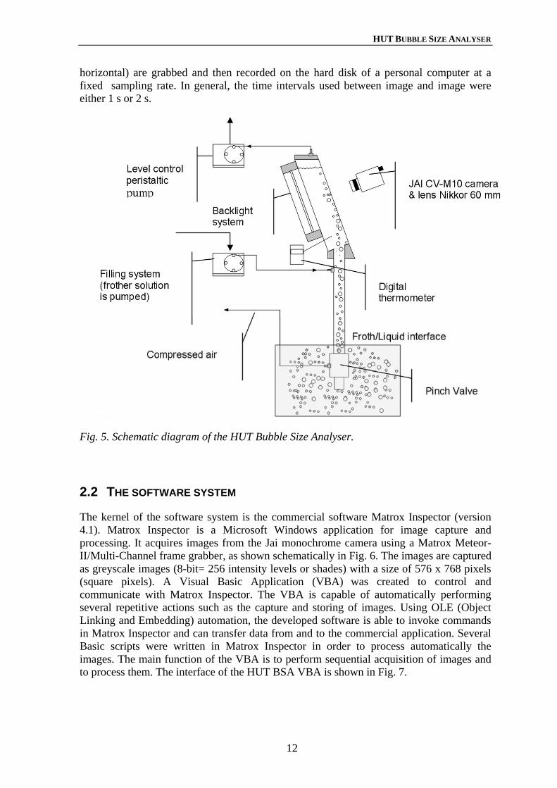
The apparatus comprises essentially a viewing chamber connected to a sampler tube of adaptable length. The sampler tube has an internal diameter of 2 cm and is made of a transparent plexiglass (Fig. 5). The lower end of the sampling tube is connected to a pinch valve. The viewing chamber is made of two sloped glass window sheets (20x15 cm and 20° angle) and PVC. The apparatus is filled with an aqueous solution of frother using a peristaltic pump. The lower end of the sampling probe is immersed into the flotation cell, below the froth/liquid interface. As the pinch valve is opened, a swarm of bubbles rises through the sampling tube reaching the viewing chamber. The bubbles rise up against the inner surface of the glass window as a single layer. The bubbles are then exposed to a video camera. As the bubbles reach the top of the chamber and burst, the excess of air is removed using a second peristaltic pump, so that a controlled level of water is maintained in the chamber. Since the water level does not decrease during bubble sampling, a down-flow of water in the sampling tube and inlet is prevented.
An inclined viewing chamber of the type suggested by Hernandez-Aguilar et al. (2004) reduces the probability of bubbles overlapping, so that the number of miscounted bubbles decreases. The inclined viewing chamber allows better setting of the focus plane. A Jai progressive scan monochrome camera (CV-M10 SX 1/2") fitted with an AF Micro Nikkor 60mm f/2.8D macro lens is used to capture images of swarms of bubbles. The shutter speed of the camera was set at 1/2000 s. An LED (Light Emitting Diodes) Backlight illumination system (Volpi, Switzerland) with a high light output is used to expose the contour of the bubbles in the swarm. The backlight system provides a uniform background. The illumination system was found not to raise the temperature in the viewing chamber during bubble sampling. A rather shallow depth of field is set for the measurements. Images of the swarm of bubbles crossing the field of view (about 12 mm vertical x 16 mm
HUT BUBBLE SIZE ANALYSER
12
horizontal) are grabbed and then recorded on the hard disk of a personal computer at a fixed sampling rate. In general, the time intervals used between image and image were either 1 s or 2 s.
Fig. 5. Schematic diagram of the HUT Bubble Size Analyser.
2.2 THE SOFTWARE SYSTEM
The kernel of the software system is the commercial software Matrox Inspector (version 4.1). Matrox Inspector is a Microsoft Windows application for image capture and processing. It acquires images from the Jai monochrome camera using a Matrox Meteor-II/Multi-Channel frame grabber, as shown schematically in Fig. 6. The images are captured as greyscale images (8-bit= 256 intensity levels or shades) with a size of 576 x 768 pixels (square pixels). A Visual Basic Application (VBA) was created to control and communicate with Matrox Inspector. The VBA is capable of automatically performing several repetitive actions such as the capture and storing of images. Using OLE (Object Linking and Embedding) automation, the developed software is able to invoke commands in Matrox Inspector and can transfer data from and to the commercial application. Several Basic scripts were written in Matrox Inspector in order to process automatically the images. The main function of the VBA is to perform sequential acquisition of images and to process them. The interface of the HUT BSA VBA is shown in Fig. 7.

HUT BUBBLE SIZE ANALYSER
13
. .
Fig. 6. Schematic diagram of the HUT BSA software system.
The following list comprises the main tasks performed by the HUT BSA Visual Basic Application:
• Capture and save sequentially numbered snapshots at a sampling rate specified by the user. The number of images to save is also indicated by the user.
• Capture and save an image of an object used to calibrate the images. It finds the object in the image and returns the average width of the object.
• Process sequentially a collection of images using the input parameters specified by the user. It saves the data associated with each image in a text file.
• Collect the data from the text files in an Excel workbook.
• Calculate several parameters related to the bubble size distribution, such as mean equivalent diameters.
Matrox Inspector
Image processing Software
Basic Scripts
HUT BSA
Visual Basic Application
Microsoft Excel
Several macros implemented in
HUT BSA are run through Excel
Report in a workbook
Matrox Frame Grabber
011001
CCD camera

HUT BUBBLE SIZE ANALYSER
14
Fig. 7. Interface of the HUT BSA Visual Basic Application.
2.3 IMAGE PROCESSING AND BLOB ANALYSIS
The image analysis procedure is shown in Fig. 8. Air bubbles rising up through the viewing chamber in an aqueous solution of a frother are shown in Fig. 8(a). The intensity values in the image are adjusted by linearly remapping these values to fill the entire intensity range (0-255). This simple operation allows the use of a global threshold value for a collection of images. This operation is known as window levelling; the result of this operation is shown in Fig. 8(b). It is clear from this figure that the background becomes lighter. The image is then segmented by thresholding the image. Thresholding is a common operation in image segmentation, and is used to convert a grey scale image to a binary image (Russ, 1990).
A grey scale image like Fig. 8(b) may be represented as a two-dimensional function, f(x,y), where x and y are spatial coordinates in a plane and the value of the function f(x,y) is the intensity of the image at any given pair of coordinates. For grey scale images, x, y and the value of the f function are discrete quantities. The function f takes only G=28=256 grey levels as described by Eq. (16). The intensity value or grey scale value l= 0 corresponds to the black colour and l= 255 is white.
255),(0 ≤≤ yxf (16)

HUT BUBBLE SIZE ANALYSER
15
Fig. 8. Image processing procedure: (a) original image, (b) window levelling operation, (c) thresholded image (T=180), (d) filling holes, (e) the objects touching the border are removed and (f) output of the blob analysis.
Thus, the digitized image may be represented as a Matrix with M rows and N columns, as described by Eq. (17). Each element of the matrix is called a pixel (Gonzalez and Woods, 1993). Each image acquired by the HUT BSA measuring technique is of the size 576 x 768 pixels. Eq. (18) represents the digital images collected by the HUT BSA.
These concepts allow us finally to define a thresholded image g(x,y) as
⎥⎥⎥⎥⎥⎥⎥⎥
⎦
⎤
⎢⎢⎢⎢⎢⎢⎢⎢
⎣
⎡
−−⋅⋅⋅−−⋅⋅⋅⋅⋅⋅
−⋅⋅⋅−⋅⋅⋅
=
)1,1()1,1()0,1(
)1,1()1,1()0,1()1,0()1,0()0,0(
),(
NMfMfMf
NfffNfff
yxf (17)
⎥⎥⎥⎥
⎦
⎤
⎢⎢⎢⎢
⎣
⎡
⋅⋅⋅−
−⋅⋅⋅⋅⋅⋅
=
)767,575()1,1()0,575(
)1,1()1,1()0,1()767,0()1,0()0,0(
),(
fMff
Nffffff
yxf (18)
⎩⎨⎧
<≥
=TyxfifTyxfif
yxg),(0),(255
),( (19)
(e) (f) (d)
(c) (b) (a)

HUT BUBBLE SIZE ANALYSER
16
where T is a constant that is commonly referred to as a global threshold value. The T value is chosen in order to separate or extract the silhouettes of the bubbles from the background. The value of the threshold in this project is determined interactively by the user. The image shown in Fig. 8(c) was thresholded using T =180. The thresholding operation produces an image that is composed of black objects, the silhouettes of the bubbles, and a white background. The thresholded image may be considered a binary image because the grey level of each pixel either takes the value 0 (black) or 255 (white).
Fig. 8(d) shows the binary image after performing the morphological reconstruction operation, filling holes procedure (Gonzalez et al., 2004). This procedure is used to eliminate open areas in the silhouettes of the bubbles due to surface reflections. This procedure also fills the core of the bubble. This operation allows bubble area measurements and reduces dramatically oversegmentation of the bubbles. Imperfections in the silhouettes of the bubbles lead to the bubbles being improperly split by the software. The objects that touch the border of the image are removed, since these structures are often incomplete bubbles, and therefore provide information unnecessary for bubble sizing. The image produced by this operation is shown in Fig. 8(e).
Once the image has been processed, (Figs. 8(a) to 8(d)), the Matrox Inspector´s blob analysis procedure is invoked. This tool allows the identification and measurement of connected regions of pixels (objects or blobs) within an image. In this case, the objects of interest are naturally the bubbles or black regions within the image. The identification of connected regions is performed by labelling the objects within the image. The result of the labelling operation depends completely on the definition of adjacency. In this project, the form of adjacency chosen is 8-connected, that is to say, if two pixels touch vertically, horizontally or diagonally, they are considered part of the same object. A pixel p and its set of 8-neighbours (8-connected) are shown in Fig. 9(a), while Fig. 9(b) shows the set of 4-neighbours of pixel p (4-connected).
Fig. 9. Types of adjacency: the shaded pixels are (a) 8-connected and (b) 4-connected.
Due to the type of sampling technique used, the overlapping of bubbles is dramatically reduced; however, it was observed that bubbles were frequently touching each other. Thus, before performing a labelling operation, it is necessary to perform an operation to separate the touching objects within the images. Touching blobs in a binary image are separated by means of a watershed algorithm. The blob analysis module automatically separates touching blobs in a binary image. The module uses a distance transform in conjunction with the watershed transform. The watershed transform is discussed in detail by Sonka et al. (1999) and Russ (1990). A more practical approach to the watershed segmentation can be found in Gonzalez et al. (2004). The outcome of the binary separation is shown in Fig. 10. The separated bubbles are outlined with red ovals in Fig. 10(b).
p p
(a) (b)

HUT BUBBLE SIZE ANALYSER
17
Fig. 10. Binary separation: (a) source image and (b) output image.
The output of the blob analysis is shown graphically in Fig. 8(f), where the selected bubbles are shown in the red overlay plane. For each object within the binary image, the maximum (Fmax) and minimum (Fmin) diameters are computed; the diameters are determined by checking the Feret diameter of the object at a specified number of angles (Fig. 11). Twenty two was the number of angles found to give accurate results for sizing the bubbles. Along with the Feret diameters, the projected area (A), perimeter of the projected bubble (Pe) and the compactness of each object are measured. The compactness (Comp) is used to measure the elongation of an object and is given by:
A disc has the minimum compactness value, which is equal to 1. This shape factor is used as the criterion for identifying clusters of bubbles that could not be separated into single objects using the processing operations. An object in an image with a compactness exceeding 1.25 is identified as a possible cluster and therefore removed from the list of identified bubbles. The compactness of assorted bubbles is shown in Fig. 12. Two equivalent diameters are calculated using the information extracted from the collection of images: the projected-area diameter (dAM) and the bubble volume-equivalent diameter (dVM). The projected area diameter is calculated as indicated in Eq. (21), and the bubble volume equivalent diameter is calculated using the maximum Feret diameter (Fmax) of the bubble and the minimum Feret diameter (Fmin), as described by Eq. (22). Note that the subscript M refers to non-corrected values, and that it indicates the diameter measured at location M, as shown in Fig. 14.
APeComp π4
2
= (20)
(a) (b)

HUT BUBBLE SIZE ANALYSER
18
Fig. 11. Feret diameters or calliper diameters in various directions. F90 and F145 correspond to the Feret diameters measured at angles of 90° and 145° respectively, while Fmin and Fmax are the minimum and maximum Feret diameters of the bubble.
As can be seen in Fig. 8(f), four objects were considered as erroneous bubbles based on the values of compactness. These objects are therefore excluded from the results. Enlargements of Fig. 8(a) and (f) are shown in Fig. 13, where the excluded objects are outlined in blue ovals. The ovals (a) and (b) seem to be bubbles that are out of focus. These are most likely bubbles attached to the back glass window of the viewing chamber. Often when the viewing chamber is being filled with the aqueous solution of the frothers, tiny bubbles attach to the glass windows. Prior to conducting any measurement, these bubbles are wiped off from the glass windows. In fact, the rising bubbles quickly sweep off any remaining bubble on the front glass window. In contrast, a remaining bubble on the back glass window could be repeatedly photographed during the sampling period. The oval (c) outlines two overlapping bubbles that are correctly removed from the sample. And the oval (d) outlines a removed object from the sample, which corresponds to an incomplete bubble, the edge of which became blurred, probably due to surface reflections.
⎟⎟⎠
⎞⎜⎜⎝
⎛=
πAd AM 2 (21)
3min
2max FFdVM = (22)
F90
F145
Fmax
Fmin
Fmax
Fmin

HUT BUBBLE SIZE ANALYSER
19
Fig. 12. Size and compactness of different bubbles.
Fig. 13. Excluded group of objects from an image based on their compactness values: (i) source image and (ii) measured bubbles in the red overlay plane.
dv= 4.02 mm and Comp = 1.20 mm
dv= 2.70 mm and Comp = 1.20
dv= 1.77 mm and Comp = 1.17
dv= 1.20 mm and Comp = 1.16
dv= 1.01 mm and Comp = 1.16
4.0 mm
3.0 mm
2.0 mm
2.0 mm
1.5 mm
1.0 mm dv= 0.55 mm and Comp = 1.16
(i) (ii)
(a)
(b)
(c) (d)
(a)
(b)
(c) (d)

HUT BUBBLE SIZE ANALYSER
20
2.3.1 Mean bubble diameters
The bubble volume equivalent diameter (dVM) and the projected-area diameter (dAM) of each bubble are calculated and stored automatically in an Excel workbook. It is in the workbook where the Sauter mean bubble diameters (d32V and d32A) and the mean number diameters (d10V and d10A) of the sample, among other parameters associated with the bubble size distribution, are calculated. The mean number diameters are calculated as indicated in Eq. (23). The Sauter mean bubble diameter is defined as the volume-to-surface mean, as described by Eq. (24). Note that the subscript M refers to non-corrected values, and that it indicates the diameter measured at location M, as shown in Fig. 14.
In this study, all the diameters are reported at standard conditions (temperature 298.15 K and pressure 101,325 Pa). The mean diameters are corrected using a correction factor CTP, as indicated in Eq. (25); in this case, the Sauter mean bubble diameter is corrected. The correction factor CTP is calculated as indicated in Eq. (26), where HM is the distance between the point at which the bubbles are photographed and the froth/liquid interface as shown schematically in Fig. 14. It is noteworthy that the correction factor CTP for measurements performed in a laboratory scale flotation cell is very close to unity. Equation (26) shows the CTP factor used for the tests conducted in a 265 dm3 Outokumpu cell (Publication VI).
N
dd
N
iVMi
VM
∑== 1
10 or N
dd
N
iAMi
AM
∑== 1
10 (23)
∑
∑
=
== N
iVMi
N
iVMi
VM
d
dd
1
2
1
3
32 or ∑
∑
=
== N
iAMi
N
iAMi
AM
d
dd
1
2
1
3
32 (24)
Fig. 14. Schematic diagram of the HUT BSA with the variables used for the calculation of the correction factor.

HUT BUBBLE SIZE ANALYSER
21
TPVMV Cdd ⋅= 3232 (25)
≈⋅= 315.298
1,033.256-1,033.256
M
MTP T
HC 0.99 (26)
2.3.2 Calibration of the images
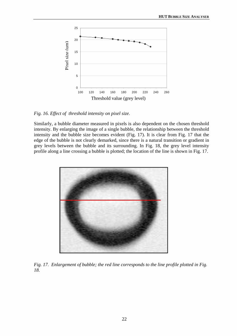
The dimension of a single pixel is calibrated by imaging an object of a known size placed across the field of view. Fig. 15 shows a syringe needle with an external diameter of 0.710 mm that has been used for calibrating the images. The calibration image is also converted into a binary image using the same threshold intensity as the one used for the segmentation of the bubbles, so accurate dimensions are assigned to each pixel in the image. Due to the type of lighting system (diffuse back lighting) used, the width of the calibration object was found to be dependent on the threshold intensity chosen for the segmentation process. The width in pixels of the projected object increased with increasing threshold intensity. Consequently, the pixel size decreased with increasing threshold intensity (Fig. 16). For instance, at a threshold intensity of 180, the pixel size is ca. 20 µm by 20 µm.
Fig. 15. Calibration image; an object of known size is photographed.
HUT BUBBLE SIZE ANALYSER
22
Fig. 16. Effect of threshold intensity on pixel size.
Similarly, a bubble diameter measured in pixels is also dependent on the chosen threshold intensity. By enlarging the image of a single bubble, the relationship between the threshold intensity and the bubble size becomes evident (Fig. 17). It is clear from Fig. 17 that the edge of the bubble is not clearly demarked, since there is a natural transition or gradient in grey levels between the bubble and its surrounding. In Fig. 18, the grey level intensity profile along a line crossing a bubble is plotted; the location of the line is shown in Fig. 17.
Fig. 17. Enlargement of bubble; the red line corresponds to the line profile plotted in Fig. 18.
0
5
10
15
20
25
100 120 140 160 180 200 220 240 260
Pixe
lsiz
e(u
m)
Threshold value (grey level) i i

HUT BUBBLE SIZE ANALYSER
23
Fig. 18. Grey level profile across the bubble.
The size of three different bubbles determined at various threshold intensities is shown in Fig. 19. It is clear from this figure that, by applying the same threshold intensity to the calibration image, the mapping procedure does not appear to have any significant effect on the size of the bubbles. Leifer et al. (2003) calibrated the pixel resolution in their experimental work using a ruler located in the plane of the rising bubbles. Naturally, they observed large differences in bubble size depending on the threshold intensity.
Fig. 19. Bubble size at various threshold intensities.
0
50
100
150
200
250
300
0 20 40 60 80 100 120 140
Gre
y le
vel i
nten
sity
Length (pixels)
0
0.5
1
1.5
2
140 160 180 200 220
Bubble 1
Bubble 2
Bubble 3
Bub
ble
diam
eter
(mm
)
Grey level intensity

HUT BUBBLE SIZE ANALYSER
24
2.4 VALIDATION STUDY
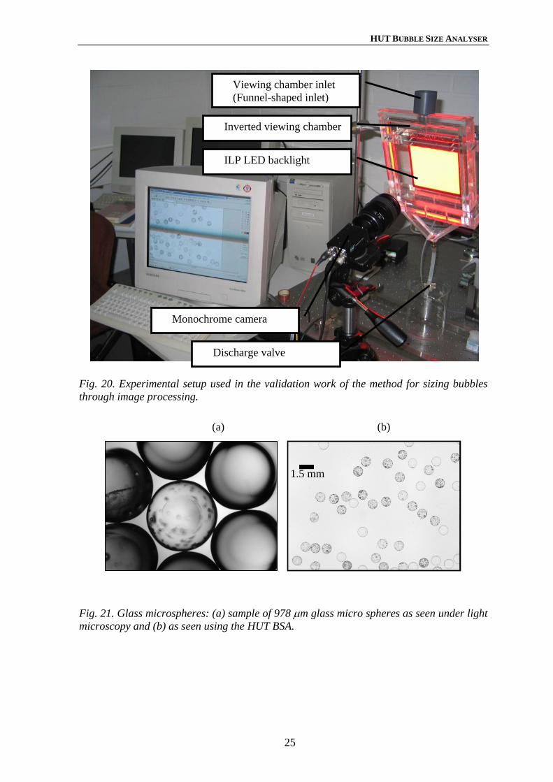
As a part of the validation work of the image analysis method, monodisperse distributions of glass microspheres (NIST traceable monodisperse standards) manufactured by Whitehouse Scientific (England) are used to study the performance of the technique. The glass spheres are dropped into an inverted viewing chamber filled with water, mimicking a swarm of bubbles. Due to the inclination of the glass window, the microspheres slide down against the inner surface of the glass window. The inverted viewing chamber was designed so that the distance from the ILP LED Backlight system to the glass windows is the same as in the original viewing chamber. The angle of inclination of the glass windows with respect to the vertical (a 20° angle) is also the same. The inverted viewing chamber is shown in Fig. 20. A sample of glass microspheres as seen under light microscopy is shown in Fig. 21(a).
In order to quantify the gauging errors introduced by the technique, various size classes of glass microspheres were sized using the HUT BSA (Fig. 21(b)). Table 2 and Table 3 show the comparison between the results given by the HUT BSA for different size classes of microspheres and the certified reference values. The absolute relative errors shown in Table 2 were calculated using the mean bubble volume equivalent diameter (d10V), while in Table 3, the errors were calculated using the mean projected-area diameter (d10A). The calculation of the absolute relative error with respect to the certified mean sizes is described by Eq. (27), where d10spheres is the certified mean size of the microspheres given by the manufacturer.
spheres
spheresV
ddd
error10
1010 −= or spheres
spheresA
ddd
error10
1010 −= (27)
HUT BUBBLE SIZE ANALYSER
25
Fig. 20. Experimental setup used in the validation work of the method for sizing bubbles through image processing.
Fig. 21. Glass microspheres: (a) sample of 978 µm glass micro spheres as seen under light microscopy and (b) as seen using the HUT BSA.
Inverted viewing chamber
Monochrome camera
ILP LED backlight
Discharge valve
Viewing chamber inlet (Funnel-shaped inlet)
1.5 mm
(a) (b)

HUT BUBBLE SIZE ANALYSER
26
Table 2. Validation study of the HUT BSA technique using glass microspheres, bubble volume-equivalent diameter.
Class number
d10spheres (µm) monodisperse
glass microspheres
d10V(µm)
HUT BSA
Standard deviation
(µm) HUT BSA
Relative Errors
1 405.9 +/-8.7 429 15.9 5.7%
2 589 +/-8. 618 16.5 4.9%
3 774 +/- 3. 752 20.2 2.80%
4 978 +/-7 988 24.4 0.99%
5 1917 +/-11 1992* 45.6 3.91*%
*The values are different from those in Publication VI because an error in the calculation was observed.
Table 3. Validation study of the HUT BSA technique using glass microspheres (projected-area diameter).
Class number
d10spheres (µm) monodisperse glass
microspheres
d10A(µm)
HUTBSA
Standard deviation
(µm) HUTBSA
Relative Errors
1 405.9 +/-8.7 415 13.8 2.2%
2 589 +/-8. 601 17.9 2.0%
3 774 +/- 3. 735 18.61 5.10%
4 978 +/-7 968 22.7 0.99%
5 1917 +/-11 1958 41.3 2.15%
It is clear from Table 2 and Table 3 that the gauging errors introduced by the technique are relatively low. In Table 2, the largest relative error is found in the finest size, Class 1, with a relative error of 5.7% (i.e. an error of approximately 23 µm). Since the pixel size used during the measurements was of ca 20 µm by 20 µm, the error can be considered fairly small. In general, the size of the microspheres was overestimated when the bubble volume equivalent diameter was used as the representative diameter. It seems that the relative error had a tendency to increase in magnitude for the smallest size classes. When the projected area diameter was used, the relative errors tended to be smaller in comparison to the relative errors shown in Table 2.
In Table 3, the largest relative deviation from the certified mean size is found in Class 3 (a relative error of 5.1%), the mean size in this particular measurement was underestimated. Table 3 shows that the diameter of the sample was slightly underestimated in two measurements and slightly overestimated in three measurements. An average relative error

HUT BUBBLE SIZE ANALYSER
27
of approximately 3.6% was observed when using the bubble volume equivalent diameter as the representative diameter, and an average error of approximately 2.5% when using the projected-area diameter. In general, the HUT BSA appears to give accurate results for all the sizes of glass microspheres examined, which are in the same range of mean bubble sizes frequently observed in laboratory-scale flotation cells.
It is noteworthy that the accuracy of the measurements is dramatically influenced by the quality of the calibration image, as was observed in the experimental work. It might be expected that the accuracy of the method is drastically increased using a monochrome camera with a higher pixel resolution. On the other hand, the acquisition, storage and analysis of higher-resolution images demand more computational power.
2.4.1 The correct threshold value
There are several potential error sources in the sizing method, but probably the most important factor is the determination of an adequate threshold value. In this section, the effect of the threshold value upon the gauging error is analysed.
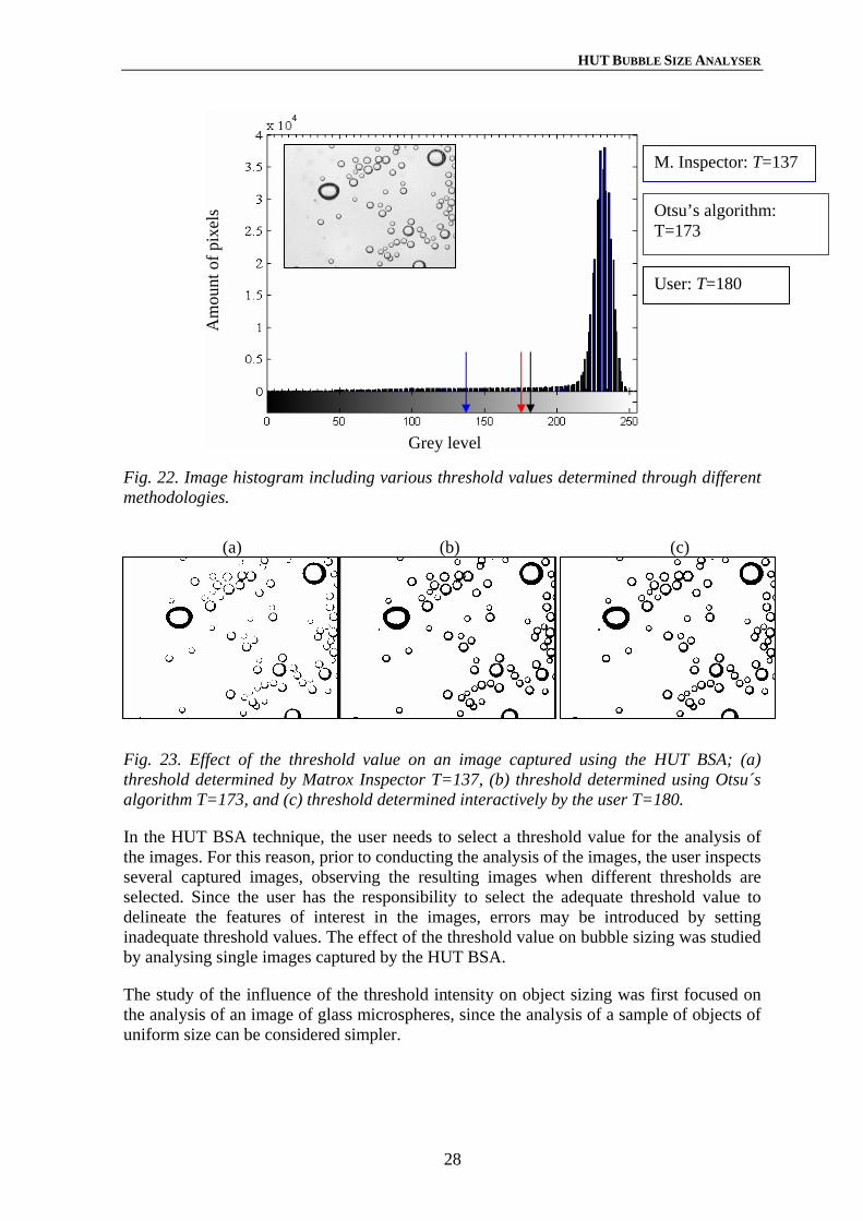
Correct threshold selection is crucial for the succesful segmentation of the captured images. This selection can be determined manually or it can be determined using a threshold determination algorithm (Sonka et al., 1999). The automatic routine implemented in Matrox Inspector for determining thresholds values was found to give poor results. The threshold value was systematically underestimated by the implemented algorithm, as shown graphically in Fig. 22. The threshold values calculated using three different methods are shown in this figure. As can be seen in Fig. 23, the threshold determined with the aid of the software produced a poor result, while the threshold values determined interactively by the user and through a global thresholding algorithm (Otsu, 1979) gave qualitatively better results. In fact, the differences between Fig. 23(b) and 23(c) are almost invisible to the naked eye. Otsu’s algorithm is implemented in the MATLAB image processing toolbox, Matworks.
HUT BUBBLE SIZE ANALYSER
28
Fig. 22. Image histogram including various threshold values determined through different methodologies.
Fig. 23. Effect of the threshold value on an image captured using the HUT BSA; (a) threshold determined by Matrox Inspector T=137, (b) threshold determined using Otsu´s algorithm T=173, and (c) threshold determined interactively by the user T=180.
In the HUT BSA technique, the user needs to select a threshold value for the analysis of the images. For this reason, prior to conducting the analysis of the images, the user inspects several captured images, observing the resulting images when different thresholds are selected. Since the user has the responsibility to select the adequate threshold value to delineate the features of interest in the images, errors may be introduced by setting inadequate threshold values. The effect of the threshold value on bubble sizing was studied by analysing single images captured by the HUT BSA.
The study of the influence of the threshold intensity on object sizing was first focused on the analysis of an image of glass microspheres, since the analysis of a sample of objects of uniform size can be considered simpler.
M. Inspector: T=137
User: T=180
Otsu’s algorithm: T=173
Am
ount
of p
ixel
s
Grey level
(a) (b) (c)

HUT BUBBLE SIZE ANALYSER
29
Fig. 24. Effect of the threshold value on the resulting image: (a) glass microspheres, original image, (b) low threshold intensity T=200, (c) adequate threshold intensity T=220, and (d) high threshold intensity T=230.
Fig. 24 shows the effect of different threshold values used on an image of glass microspheres. The image was randomly picked from the experiments carried out with glass microspheres. Fig. 25 shows the effect of the threshold value on three parameters: the number of glass microspheres identified, number of glass microspheres miscalculated and the relative error of the measurement. The relative errors plotted in Fig. 25 were computed using the number mean diameters (d10V), as indicated in Eq. (27).
As can be observed in Fig. 25, as the threshold value was increased, there was a marked rise in the number of blobs detected, reaching the highest values at threshold intensities between 215 and 220. With further increases in threshold intensity, the number of glass microspheres sized decreased. The relative error decreased dramatically with increasing threshold intensity. The relative error was found to be less than 3.5% at threshold intensities higher than the grey scale level 210. Similar behaviour was observed with the number of miscalculated objects or blobs in the image: the number of objects miscalculated decreased with an increase in threshold intensity. Miscalculated objects are either oversegmented, glass microspheres improperly divided, or clusters of microspheres recognised as a single element. It is worthy of note that 80 glass microspheres were manually identified in the image. Consequently, the technique was not able to recognize the totality of glass microspheres in the image.
(a) (b)
(c) (d)

HUT BUBBLE SIZE ANALYSER
30
Fig. 25. Effect of the threshold on image analysis of glass microspheres. Eighty glass microspheres were manually identified.
Similar behaviour was observed for an image of bubbles captured using the HUT BSA. Fig. 26 shows the effect of the threshold intensity on bubble sizing. The number of bubbles increased rapidly with increasing threshold intensity, reaching the highest values at threshold intensities between 170 and 200. The number of bubbles identified decreased dramatically at threshold values higher than 200.
At threshold intensities between 170 and 200, the relative error on the average bubble diameter (d10V) and Sauter mean bubble diameter (d32V) were found to be small (relative error < 5%). However, outside this range, the relative errors were extremely high. The reference values used in the calculation of the relative errors (Eq.(28)) were manually determined. Thus the reference average bubble size ( *
10Vd ) and Sauter mean bubble diameter ( *
32Vd ) were calculated from data measured with the use of a calliper.
*10
*1010100
V
VV
ddd
error −= or *32
*3232100
V
VV
ddd
error −= (28)
Fig. 27 shows the impact of the threshold intensity on the analysis of a collection of images (500 images). The number of bubbles sized - threshold intensity curve has the same shape as the curves shown in Figs. 25 and 26. In addition, the average bubble diameter (d10V) and the Sauter mean bubble diameter (d32V) were observed to level off, in the range where the number of bubbles sized reaches the highest values. This set of results seems to indicate that there exists a range of threshold intensities that will provide an adequate measurement of bubble size. This range appears to be easy to detect interactively by the user.
Num
ber o
f gla
ss m
icro
sphe
res
0
10
20
30
40
50
60
70
80
195 200 205 210 215 220 225 230 2350
10
20
30
40
50
60
70
80
Number of glass microspheres
Miscalculated glass microspheres
Percentage error
Rel
ativ
e er
ror (
%)
Threshold value

HUT BUBBLE SIZE ANALYSER
31
Fig. 26. Effect of the threshold on the image analysis of a randomly picked image of bubbles (number of bubbles manually sized 59).
Fig. 27. Effect of threshold intensity on the image analysis of 500 images.
The outcome of the experiments would also indicate that a global threshold can not be used for a collection of images that have been taken under different lighting conditions, since large gauging errors could be introduced by the method. In that case, threshold intensities should be determined for each image with the use of an automatic determination method. In preliminary tests with floatable solids, it was observed that the viewing chamber of the HUT BSA darkened quickly as solids were released when bubbles burst as they reached the top of the chamber. Consequently, the presence of solids caused variations in the lighting conditions in the viewing chamber during sampling.
Threshold value
0
10
20
30
40
50
60
100 120 140 160 180 200 220 2400
10
20
30
40
50
60
Number of blobs
Error d32V
Error d10V
Num
ber o
f bub
bles
size
d
Rel
ativ
e er
ror (
%)
Num
ber o
f bub
bles
size
d
Bub
ble
size
(mm
)
Threshold value
0
10,000
20,000
30,000
40,000
50,000
60,000
100 120 140 160 180 200 220 2400
0.25
0.5
0.75
1
1.25
1.5
Number of bubbles
d32V
d10V

HUT BUBBLE SIZE ANALYSER
32
In the preliminary tests conducted with floatable solids, coarse particles of quartz were floated with Flotigam EDA (Clariant GmbH) as collector (100 g/t), the tests were carried out in a 50 dm3 Outokumpu cell. These tests were conducted to evaluate the ability of the HUT BSA to measure bubble size in the presence of floatable solids. Although this experimental work will not be discussed in any detail in this thesis, it should be remarked that bubbles were observed to preferentially rise as bubble clusters that were held together by hydrophobic particles (see Fig. 3). The presence of these clusters made the analysis of the images extremely difficult.
2.4.2 Effect of compactness
Despite the fact that a separating algorithm is applied to each image to split touching bubbles, i.e. bubbles in clusters, often the algorithm failed to efficiently split each cluster into single bubbles. Thus, the compactness parameter was selected as a criterion for identifying possible remaining clusters. If the compactness of an object exceeds a critical value, the object is identified as a possible cluster and therefore removed from the sample. It was found that a critical value of 1.25 produced adequate results. Fig. 28 shows the impact of the critical value on the measurement of glass microspheres. During the tests, a threshold intensity of T=218 was applied to the image. The critical compactness turned out to be an efficient criterion to recognize oversegmented blobs, or objects out of focus. It is clear from Fig. 28 that, at critical values exceeding 1.25, the number of glass microspheres reached values over 80 units, which exceeds the real number of glass microspheres present in the image (80 units). The source of this error is mainly due to oversegmentation.
Fig. 28. Effect of the compactness on sizing glass microspheres.
Rel
ativ
e er
ror (
%)
0
20
40
60
80
100
120
1 1.2 1.4 1.6 1.8 20
5
10
15
20
25
30
Number of glass microspheres Miscalculated glass microspheres
Relative error
Num
ber o
f blo
bs si
zed
Critical compactness

HUT BUBBLE SIZE ANALYSER
33
2.4.3 Number of bubbles sampled
The minimum number of bubbles that should be sized in order to determine accurately the Sauter mean diameter depends on the distribution itself. Irani and Callis (1963) suggested that the number of particles (bubbles) measured should be large enough so that the results do not change on measuring a larger number. This concept is graphically shown in Fig. 29. As can be seen from this figure, a minimum of 1500 of bubbles should be sized. In the experimental work reported throughout Publications I, II, III, IV and VI, the number of bubbles sized was in fact, on average, several times larger than the number inferred from Fig. 29. This was because a larger number of bubbles sized produces a more accurate measurement of the entire bubble size distribution, i.e. the number of bubbles in each size class increases.
Fig. 29. Bubble size as a function of the number of bubbles characterized.
Bub
ble
size
(mm
)
Number of bubbles sized
0
0.2
0.4
0.6
0.8
1
1.2
1.4
0 2000 4000 6000 8000 10000
d32V
dv10
Stdev
d10 STDEV d32

EXPERIMENTAL
34
3 EXPERIMENTAL
3.1 LABORATORY-SCALE FLOTATION CELLS
Three Outokumpu cylindrical laboratory-scale cells were used throughout the experimental work. The main specifications of the individual cells are listed in Table 4.
Table 4. Specifications of laboratory flotation cells used throughout the experimental work.
Cell name
Nominal volume (dm3)
Tank diameter DCell (mm)
Liquid height (mm)
Impeller diameter DI (mm)
Type of mechanism fitted
Other features
OK-50 50 350 350 125 Multi-Mix Four baffles, cell made of stainless steel
OK-70 70 420 420 108 Multi-Mix and Free-Flow
Transparent cell made of plexiglass
OK-265 265 650 650 150 Multi-Mix and Free-Flow
Transparent cell made of plexiglass
The 265 dm3 Outokumpu flotation cell, from now on referred to as OK-265 in keeping with the names given in Table 4, is shown in Fig. 30. The 70 dm3 cell, from now on referred to as OK-70, is shown in
Fig. 31. The OK-265 cell is enclosed in a plexiglass open-top box that is filled with water during the experiments to make visualization of the flow and gas dispersion conditions in the cell possible. A special launder made also of plexiglass is designed to collect the foam overflowing the lip of the cell. This cell is designed to carry out mainly gas-liquid (two-phase system) experiments.
A series of tests were conducted in a 1 dm3 Open-Top Leeds flotation cell, these tests are reported in Chapter 4 and in more detail in Publication III. The experimental work carried out in the Open-Top Leeds flotation cell was performed by, or under direct supervision of Laskowski (Publication III).
3.1.1 Air flow rate
In Outokumpu cells, air is introduced through a hollow shaft. The air flow rate entering the cell was continuously measured using rotameters (Kytola, Finland). The air flow rate measurements were corrected according to the working pressure and are reported at standard conditions (temperature 25°C and pressure 101,325 Pa). Note that the aeration conditions in the cells are often reported in terms of the overall superficial gas velocity (Jg), which is calculated as indicated in Eq. (29), where Qg is the air flow rate and Ac the cross-sectional area of the cell.

EXPERIMENTAL
35
Fig. 30. Laboratory scale flotation cell OK-265, fitted with a Free-Flow mechanism.
c
gg A
QJ =
(29)
Air inlet chamber
Torque sensor

EXPERIMENTAL
36
Fig. 31. Laboratory scale flotation cell OK-70, fitted with a Multi-Mix mechanism.
3.1.2 Rotor/stator mechanisms
Two types of commercial rotor/stator mechanisms manufactured by Outokumpu, Multi-Mix and Free-Flow mechanisms, were used in the tests.
Fig. 32. Rotor/stator mechanisms: (from left to right) Free-Flow mechanisms, Multi-Mix mechanism and a closer look at the Outokumpu rotor OK with the Free-Flow stator.
3.1.3 Impeller speed
In general, the rotational speed of the rotor is controlled by a variable speed drive; here, it was also measured using digital (optical) tachometers.
Torque table or Turntable

EXPERIMENTAL
37
The impeller speed in the OK-50 was set using a variable speed drive; the impeller speed was verified using a hand digital tachometer (Shimpo EE-2) with an accuracy of 1 rpm.
The rotational speed of the mechanism in the OK-265 is controlled by an ABB AC drive (ACS 800). The rotational speeds were verified using a hand digital tachometer (Shimpo EE-2) and a stroboscope (accuracy:±0.05% +1 digit).
3.1.4 Power measurements
The power drawn by the OK-70 cell mechanism was determined by measuring the torque experienced by the cell (mixing vessel) in reaction to the rotating impeller; in this case the liquid acted as a transmitting medium. The cell is supported (mounted) on a thrust bearing (torque table), as shown in
Fig. 31. The torque experienced by the cell is determined with the use of a strain gauge. The power drawn by the mechanism is calculated as follows:
30Iq
draw
NTP
⋅⋅=
π (30)
where Tq is the torque value in units of N⋅m, NI the rotational speed of the impeller in rpm and Pdraw the power in Nm/s (Watt). Power measurements in the OK-70 cell are reported in Publication IV.
In the OK-265 cell, the power drawn by the cell mechanism was determined by measuring the torque experienced by the rotating shaft. An HBM T20WN/200 torque sensor is utilised for the measurements. Torque values are determined by measuring the elastic deformation of the shaft by the change in electrical resistance. The T20WN/200 torque transducer is installed as a support bearing, located above the air inlet chamber (see Fig. 30). The signals from the sensor were collected using a HBM amplifier system (MP60), and the data logged into a PC (into an Excel file) for analysis. Since the air inlet chamber comprises a bearing system for the rotating shaft, friction is introduced by the bearing system and causes power dissipation. Thus, friction causes some of the torque transmitted to the cell mechanism (rotor) to be lost. Consequently, the actual power drawn by the rotor is calculated by subtracting the power measured with the rotor running free (empty cell, i.e. rotor in air) from the power measured with the cell operating with liquid, as shown graphically in Fig. 33. It is noteworthy that a linear equation can be fitted to the power dissipated by friction. The power data shown in Fig. 33 were calculated using Eq. (30).
3.1.5 Temperature of the liquid
The temperature of the liquid in the flotation cell was continuously monitored during the experimental work. All the tests were run at room temperature. In a turbulent flow, there is a considerable dissipation of energy, which is converted to heat. Thus, the temperature of the liquid in the cell tended to rise during the experimental work.

EXPERIMENTAL
38
Fig. 33. Power measurements conducted in the OK-265 cell running free and with the rotor operating under load (without aeration). The cell was fitted with the Multi-Mix mechanism.
3.1.6 Surface tension
A Du Nouy Ring Tensiometer was used to measure the surface tension of aqueous solutions at varying frother concentrations.
3.1.7 Dynamic surface tension
Surface tension was measured dynamically using the commercial KSV BPA-800P maximum bubble pressure tensiometer.
3.1.8 High-speed imaging system
Videos of the cell mechanisms were captured using the Photron’s Ultima APX fast camera. This camera was kindly lent by RTS Cheos Oy (Finland). The camera was operated by an expert from Photron Europe Limited. Most of the videos were captured through the transparent base of the OK-265 cell, and they were recorded during the onset of aeration.
0
500
1000
1500
2000
2500
3000
3500
100 300 500 700 900 1100 1300
Power dissipated by friction
As measured
Corrected power draw
Fitted curve
Power dissipated by friction (fitted)
Pdraw=0.41•N 2.94 Pow
er c
onsu
mpt
ion
(W)
Impeller speed NI (rpm)

EXPERIMENTAL
39
3.2 BUBBLE SIZE MEASUREMENTS
The experiments were carried out in a batch mode. The level of liquid in each cell was set equal to the diameter of the cell; the total volume of tap water added to each cell is listed in Table 5. In the tests, the hydrodynamic conditions in the cell were altered by modifying the aeration rate and impeller speed. The operating conditions set in each cell are also listed in Table 5.
Table 5. Operating conditions in the laboratory flotation cells.
Cell name
Type of mechanism
Impeller Speed NI (rpm)
Impeller tip speed TS (m/s)
Power consumption (kW/m3)
Gas velocity Jg (cm/s)
Liquid Volume (dm3)
OK-50 Multi-Mix 250-1100 1.6-7.2 Not measured 0.5-1.7 30
OK-70 Multi-Mix 610-700 3.4-4.0 0.4-0.6 1.4 60
OK-70 Free-Flow 650-770 3.7-4.4 0.45-0.55 1.4 60
OK-265 Multi-Mix 300-900 2.4-7.1 0.15-2.46 0.5-2.0 215
OK-265 Free-Flow 300-900 2.4-7.1 0.14-3.5 0.5-2.0 215
All the tests were conducted with three commercial Dow frothers (Table 6). The required volume of frother was added from stock solutions (around 10 g/dm3). In the tests run in the OK-265 cell, owing to the large volume of water used in the experiments, the cell was emptied and then refilled with fresh water only if the temperature of the water exceeded 25°C. At temperatures below 25°C, only the amount required for increasing the concentration to a new value was added. In the tests carried out in the OK-50 cell, fresh water was always used for preparing a new frother solution.
The OK-70 cell was filled with only aqueous solutions of DF-250.
Table 6. List of frothers, the acronym DF stands for the trade name Dowfroth.
Common name Chemical formula Molecular weight
DF-200 CH3(OC3H6)3OH 206.29
DF-250 CH3(OC3H6)4OH 264.37
DF-1012 CH3(OC3H6)6.3OH 397.95
Bubble size distributions were determined using the HUT BSA. The bubble viewer chamber was always filled with the same frother solution as in the cell, at the same frother concentration as in the cell.

EXPERIMENTAL
40
In general, bubbles were sampled from the cell, once the foam reached a stable level in the cell. Bubbles were sampled exclusively from only one location in the cell. Images of the swarm of bubbles were captured once a steady state flow of bubbles was achieved. Bubbles were sampled for several minutes before launching the recording process. Each measurement was at least duplicated. On average, more than 5000 bubbles were sized in each recording session. The images were captured at a fixed rate with either 1 s or 2 s intervals between images. Thus, the process of acquisition of images lasted for at least 8.5 min. The sampling locations in the OK-50 and OK-70 cells are shown schematically in Fig. 34. For the tests reported in this summary, bubbles in the OK-265 cell were sampled exclusively from location 1, as shown in Fig. 35. Note that a study of the effect of the sampling location on bubble size is reported in Publication VI.
The mean diameters reported in Section 4 were calculated using the bubble volume-equivalent diameters of the bubbles.
Fig. 34. Sampling locations in the (a) OK-50 and (b) OK-70 flotation cells.
Fig. 35. Measurement locations in the OK-265 cell.
350
mm
225m
m
Bubble sampler system
420
mm
25
0 m
m
(a)
(b) Liquid level
Liquid level
65 cm
80 c
m
10 c
m20
cm
20 c
m
10 cm
65 c
m
1
2
3
Liquid level

RESULTS AND DISCUSSION
41
4 MAIN RESULTS AND DISCUSSION
4.1 EFFECT OF FROTHERS ON BUBBLE SIZE
In order to investigate the effect of frother on bubble size, two series of tests were carried out: one at the Helsinki University of Technology using an Outokumpu flotation cell, and the other at the University of British Columbia using an Open-Top Leeds lab flotation cell. In the former, the HUT Bubble Size Analyser was utilized, while the UCT bubble meter was used in the latter. The tests were carried out with the three commercial Dow frothers listed in Table 6.
In the tests carried out at Helsinki University of Technology, the experimental work was conducted in the OK-50 cell. All the experiments were carried out at room temperature. The impeller speed was set at 1050 rpm (tip speed of 6.9 m/s) and the air flow rate was set at 77 dm3/min (superficial gas velocity Jg = 1.3 cm/s). On average, about 4800 bubbles were sized in each run, and each measurement was at least duplicated. The cell was filled with aqueous solutions of the tested frother, which were prepared using municipal tap water. More details of the experimental work are presented in Section 3.2.
In the tests conducted in the 1 dm3 Open-Top Leeds lab flotation cell, aqueous solutions of the tested frothers were prepared using distilled water. The impeller speed was set at 1000 rpm and the air flow rate at 5 dm3/min (superficial gas velocity, Jg = 0.43 cm/s). A glass capillary sampler of 0.8 mm in inner diameter was fitted to the UCT Bubble Size Analyser for the experimental work. The bubble sampler of the UCT bubble size meter was positioned 50 mm above the stator. All the tests were conducted at room temperature (21 ±1 °C), and approximately 3000 bubbles were sampled for each run. The flotation cell was operated in batch mode.
The results of the measurements are shown in the form of bubble size vs. frother concentration curves in Figs. 36 to 38. The initial concentration of frother (before aeration) was used to build the bubble size vs. frother concentration curves. As these figures reveal, each curve is clearly divided into two concentration ranges, the low concentration range, which can be approximated by a steep linear fit, and the flat horizontal portion. The intersection of the horizontal asymptote to the Sauter bubble size – concentration curve with the steep linear portion can easily be determined. This is the so-called Critical Coalescence Concentration (Cho and Laskowski, 2002a, 2002b). Only the curve for DF-200 frother obtained using the HUT method (Fig. 36) is not linear over the whole concentration range from Cfo (lowest concentration of frother used in the test) to CCC. In this case, two linear portions could be identified over the Cfo to CCC concentration range, and in line with the adopted principle, the intersection of the linear portion that meets the horizontal asymptote is used to determine the CCC. The rationale followed for determining the CCC points is explained in detail in Publication VI.

RESULTS AND DISCUSSION
42
Fig. 36. Graphical determination of the CCC values for Dowfroth 200.
Fig. 37. Graphical determination of the CCC values for Dowfroth 250.
0
0.5
1
1.5
2
2.5
3
3.5
4
0 0.04 0.08 0.12 0.16 0.2
0 0.04 0.08 0.12 0.16 0.2
UCT HUT
Saut
er m
ean
diam
eter
(mm
)
Concentration (mmol/dm3)
Concentration (mmol/dm3)
0
0.5
1
1.5
2
2.5
3
3.5
4
0 0.04 0.08 0.12 0.16 0.2 0.24 0.280
0.5
1
1.5
2
2.5
3
3.5
40 0.04 0.08 0.12 0.16 0.2 0.24 0.28
UCT HUT
Saut
er m
ean
diam
eter
(mm
)
Concentration (mmol/dm3)
Concentration (mmol/dm3)

RESULTS AND DISCUSSION
43
Fig. 38. Graphical determination of the CCC values for Dowfroth 1012.
The experimentally determined CCC values for the tested frothers are given in Table 7. It is noteworthy that, despite the differences in the size of bubbles as measured using the HUT method and the UCT method, very similar CCC values were obtained in these two series of measurements.
Table 7. CCC values for the investigated frothers.
Indeed, Figs. 36 to 38 show clear trends: all the experimental bubble size vs. frother concentration curves have the same shape, irrespective of the method used to measure bubble size. They also reveal characteristic differences. The bubble sizes obtained from the extrapolation of the horizontal asymptotes for the UCT measurements give very similar bubble size values for all three tested frothers. When the HUT method was used for all three tested frothers, larger bubbles were measured.
Frother CCC, HUT technique CCC, UCT technique
mmol/dm3 ppm mmol/dm3 ppm
DF-200 0.067 13.8 0.084 17.3
DF-250 0.035 9.1 0.033 8.7
DF-1012 0.017 6.6 0.015 6.0
0
0.5
1
1.5
2
2.5
3
3.5
4
0 0.02 0.04 0.06 0.080.0
0.5
1.0
1.5
2.0
2.5
3.0
3.5
4.00 0.02 0.04 0.06 0.08
UCT HUT
Saut
er m
ean
diam
eter
(mm
)
Concentration (mmol/dm3)
Concentration (mmol/dm3)

RESULTS AND DISCUSSION
44
There may be many reasons for these differences. First, the two series of tests were carried out in different flotation machines. Also, whereas tap water was used in the HUT measurements, distilled water was used in the UCT measurements. In spite of these differences, almost identical CCC values were obtained. This implies that the CCC values for a given frother are independent of the type of machine or mechanism used for dispersing the air and independent of the operating conditions (air flow rate and impeller speed) in the cell.
The primary factors that determine bubble size include the following: bubble generating system (its geometry and hydrodynamics) and superficial gas flow rate. The secondary factors, which, in practice, may be more important than the primary ones, include, most importantly, bubble coalescence, which is determined by frother concentration (Cho and Laskowski, 2002a, 2002b).
The two utilized flotation cells, the Outokumpu cell and the Open-Top Leeds cell, have different rotor/stator mechanisms. In addition, they were operated under different conditions, with a superficial gas velocity Jg=0.43 cm/s in the Open-Top Leeds cell when the UCT method was used to follow bubble size, and Jg=1.3 cm/s in the Outokumpu cell when HUT method was utilized to follow the bubble size. The air flow rate (superficial gas velocity Jg) may have a large impact on bubble size in mechanical cells, as described in Section 4.3. Because of these differences, it is difficult to identify all the reasons that may be responsible for dissimilarities in the sizes of bubbles. Nevertheless, the following is obvious: in the case of the UCT bubble meter, the size of the bubbles at frother concentrations exceeding the CCC seems to be determined to a large extent by the measuring method. Therefore, the differences in bubble sizes over the Cf>CCC concentration range is very small for all the three tested frothers. These differences are quite substantial for the measurements carried out using the HUT bubble sizing equipment. It is surprising that the least surface-active frother, the DF-200 (Fig. 36), produced the finest bubbles, and that the largest bubbles were measured when the most surface-active frother, DF-1012, was used (Fig. 38).
Fig. 39 shows surface tension isotherms for DF-200, DF-250 and DF-1012 frothers. Comparison of the surface tension data with the CCC values given in Table 7 indicates that, while for the DF-200 frother the surface tension at the CCC concentration for this frother (8.4x10⁻⁵ M) is almost that of pure water, the surface tension for DF-250 at its CCC value (3.3x 10⁻⁵ M) is about 66 mN/m and for the DF-1012 (CCC = 1.5x10⁻⁵ M) it is about 61 mN/m. And since the slopes of the curves in Fig. 39 (b) are interrelated with adsorption via the Gibbs adsorption isotherm (see Gibbs adsorption equation, Eq (31) ), this means that the adsorption of DF-1012 at its CCC is larger than the adsorption of DF-250 at its corresponding CCC values; in turn, the adsorption of DF-250 is much greater than the adsorption of DF-200 at their respective CCC values. Yet, the finest bubbles were measured with the DF-200 frother and the coarsest with the DF-1012 frother. It follows, then, that the adsorption for larger (and more surface-active) molecules of propylene polyglycols must be greater to prevent bubbles from coalescing. This conclusion may be taken as indicating that the “static” surface tension measurements cannot be directly utilized in the analysis of the properties of dynamic systems (e.g. bubble generation).
)(3.21
fCdLogd
RTmγ
−=Γ (31)
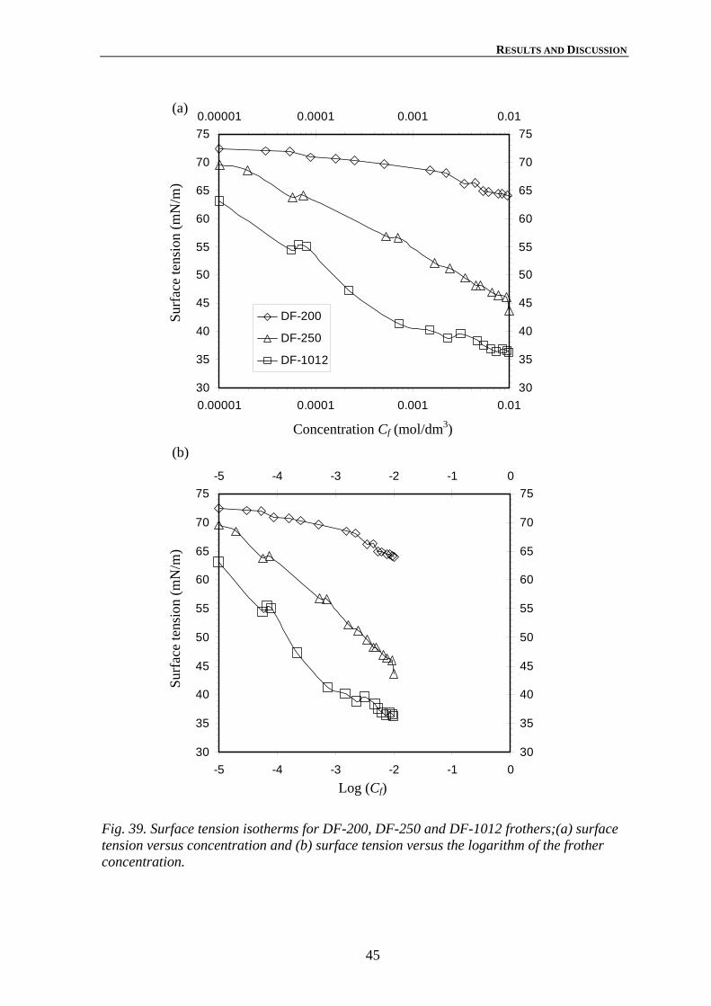
RESULTS AND DISCUSSION
45
Fig. 39. Surface tension isotherms for DF-200, DF-250 and DF-1012 frothers;(a) surface tension versus concentration and (b) surface tension versus the logarithm of the frother concentration.
30
35
40
45
50
55
60
65
70
75
0.00001 0.0001 0.001 0.0130
35
40
45
50
55
60
65
70
750.00001 0.0001 0.001 0.01
DF-200
DF-250
DF-1012
Surf
ace
tens
ion
(mN
/m)
Concentration Cf (mol/dm3)
30
35
40
45
50
55
60
65
70
75
-5 -4 -3 -2 -1 030
35
40
45
50
55
60
65
70
75-5 -4 -3 -2 -1 0
Surf
ace
tens
ion
(mN
/m)
Log (Cf)
(a)
(b)

RESULTS AND DISCUSSION
46
4.1.1 Role of frothers in bubble coalescence and bubble generation
A series of new experiments were carried out in the largest flotation cell (OK-265) in order to examine the source of differences in the bubble sizes measured using the HUT analyser in the previous tests. Only the frothers DF-200 and DF-1012 were chosen for the tests. A summary of the most important results is given in this section, while a more detailed discussion of the results of this research is given in Publication VI.
In the frother tests, the hydrodynamic conditions in the cell were altered by modifying the aeration rate and impeller speed. The impeller speed was set at 600 rpm (tip speed of 4.7 m/s) and 900 rpm (tip speed of 7.1 m/s) and the air flow rate was set at either 99 dm3/min (Jg=0.5 cm/s) or 197 dm3/min (Jg=1.0 cm/s) in the cell. The concentration of DF-200 was varied from 0.01 to 0.19 mmol/dm3 and that of DF-1012 from 0.005 to 0.075 mmol/dm3.
The effect of the Dow frothers DF-200 and DF-1012 on bubble size under varying aeration conditions at constant impeller speed (Multi-Mix mechanism) is shown in Figs. 40 and 41. These experimental data can also be fitted with two linear sections with the intersection giving the critical coalescence concentration (CCC). While for the DF-1012 frother bubble size over the non-coalescing range depends clearly on aeration conditions, the differences are negligible for the DF-200 frother. Figs. 40 and 41 include experimental data measured in the OK-50. The narrow bands in these figures illustrate the range over which the Critical Coalescence Concentration varies.
Fig. 40. Effect of DF-1012 frother concentration on bubble size at different aeration rates in the Outokumpu flotation cell fitted with a Multi-Mix mechanism. Note: TS is the abbreviation for impeller tip speed.
0
0.5
1
1.5
2
2.5
3
3.5
4
0 0.01 0.02 0.03 0.04 0.05 0.06 0.07 0.080.0
1.0
2.0
3.0
4.00 0.01 0.02 0.03 0.04 0.05 0.06 0.07 0.08
Jg=0.5 cm/s and TS=7.1 m/s, OK 265 dm3
Jg=1.0 cm/s and TS=7.1 m/s, OK 265 dm3
Jg=1.3 cm/s and TS=6.6 m/s, OK 50 dm3
Saut
er m
ean
diam
eter
(mm
)
Concentration (mmol/dm3)
Concentration (mmol/dm3)

RESULTS AND DISCUSSION
47
Fig. 41. Effect of DF-200 frother concentration on bubble size at different aeration rates in the Outokumpu flotation cell fitted with a Multi-Mix mechanism.
CCC values determined for different hydrodynamic conditions generated in the OK-265 cell, using different mechanisms and different impeller speeds, are given in Tables 8 and 9. These CCC were obtained graphically from the experimental bubble size vs. frother concentration curves as shown in Publication VI.
Table 8. CCC values for the DF-1012, measured in the OK-265 cell equipped with two different rotor /stator mechanisms operated at different impeller speeds.
Frother: DF-1012
CCC, Jg=0.5 cm/s CCC, Jg=1.0 cm/s
Multi-Mix Impeller speed (rpm) mmol/dm3 ppm mmol/dm3 ppm 600 rpm (TS=4.7 m/s) 0.017 6.8 0.019 7.6 900 rpm (TS=7.1 m/s) 0.018 7.2 0.018 7.2
Free-Flow Impeller speed (rpm) mmol/dm3 ppm mmol/dm3 ppm 600 rpm (TS=4.7 m/s) 0.017 6.8 0.020 8.0 900 rpm (TS=7.1 m/s) 0.017 6.8 0.020 8.0
CCC average 0.017 6.8 0.019 7.6
Concentration (mmol/dm3)Sa
uter
mea
n di
amet
er (m
m)
Concentration (mmol/dm3)
0
0.5
1
1.5
2
2.5
3
3.5
4
0 0.02 0.04 0.06 0.08 0.1 0.12 0.14 0.16 0.18 0.20
0.5
1
1.5
2
2.5
3
3.5
40 0.02 0.04 0.06 0.08 0.1 0.12 0.14 0.16 0.18 0.2
Jg=0.5 cm/s and TS=7.1 m/s, OK 265 dm3
Jg=1.0 cm/s and TS=7.1 m/s, OK 265 dm3
Jg=1.3 cm/s and TS=6.6 m/s, OK 50 dm3
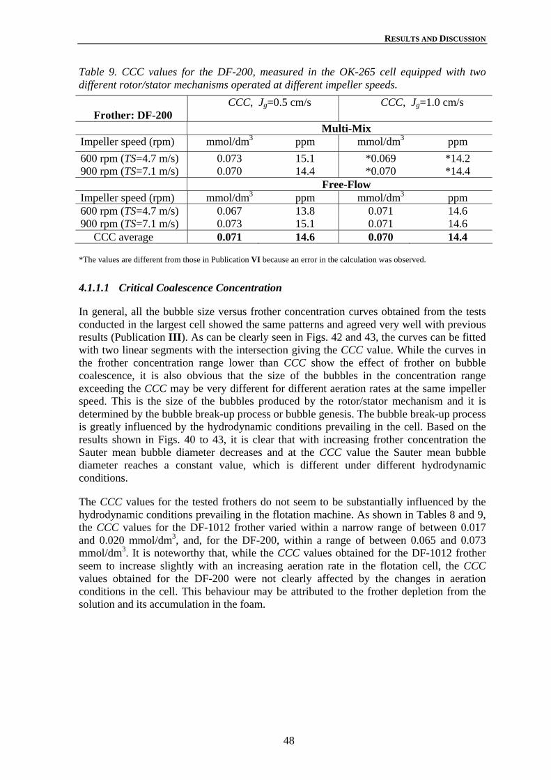
RESULTS AND DISCUSSION
48
Table 9. CCC values for the DF-200, measured in the OK-265 cell equipped with two different rotor/stator mechanisms operated at different impeller speeds.
*The values are different from those in Publication VI because an error in the calculation was observed.
4.1.1.1 Critical Coalescence Concentration
In general, all the bubble size versus frother concentration curves obtained from the tests conducted in the largest cell showed the same patterns and agreed very well with previous results (Publication III). As can be clearly seen in Figs. 42 and 43, the curves can be fitted with two linear segments with the intersection giving the CCC value. While the curves in the frother concentration range lower than CCC show the effect of frother on bubble coalescence, it is also obvious that the size of the bubbles in the concentration range exceeding the CCC may be very different for different aeration rates at the same impeller speed. This is the size of the bubbles produced by the rotor/stator mechanism and it is determined by the bubble break-up process or bubble genesis. The bubble break-up process is greatly influenced by the hydrodynamic conditions prevailing in the cell. Based on the results shown in Figs. 40 to 43, it is clear that with increasing frother concentration the Sauter mean bubble diameter decreases and at the CCC value the Sauter mean bubble diameter reaches a constant value, which is different under different hydrodynamic conditions.
The CCC values for the tested frothers do not seem to be substantially influenced by the hydrodynamic conditions prevailing in the flotation machine. As shown in Tables 8 and 9, the CCC values for the DF-1012 frother varied within a narrow range of between 0.017 and 0.020 mmol/dm3, and, for the DF-200, within a range of between 0.065 and 0.073 mmol/dm3. It is noteworthy that, while the CCC values obtained for the DF-1012 frother seem to increase slightly with an increasing aeration rate in the flotation cell, the CCC values obtained for the DF-200 were not clearly affected by the changes in aeration conditions in the cell. This behaviour may be attributed to the frother depletion from the solution and its accumulation in the foam.
Frother: DF-200
CCC, Jg=0.5 cm/s CCC, Jg=1.0 cm/s
Multi-Mix Impeller speed (rpm) mmol/dm3 ppm mmol/dm3 ppm 600 rpm (TS=4.7 m/s) 0.073 15.1 *0.069 *14.2 900 rpm (TS=7.1 m/s) 0.070 14.4 *0.070 *14.4
Free-Flow Impeller speed (rpm) mmol/dm3 ppm mmol/dm3 ppm 600 rpm (TS=4.7 m/s) 0.067 13.8 0.071 14.6 900 rpm (TS=7.1 m/s) 0.073 15.1 0.071 14.6
CCC average 0.071 14.6 0.070 14.4

RESULTS AND DISCUSSION
49
Fig. 42. Graphical determination of the CCC values for DF-200 at different aeration rates in the OK-265 cell fitted with a Multi-Mix mechanism OKMM.
Fig. 43. Graphical determination of the CCC values for DF-1012 at different aeration rates in the OK-265 cell fitted with a Multi-Mix mechanism OKMM.
As shown in Fig. 44, the dynamic surface tension - bubble life time isotherms exhibit large differences for the tested frothers. For the less surface-active frother, the dynamic surface tension data obtained from the collected samples of the foam and solution are almost identical, indicating that the foam and solution (liquid phase) were in equilibrium. For the
Saut
er m
ean
diam
eter
(mm
)
Concentration (mmol/dm3)
Concentration (mmol/dm3)
0
0.5
1
1.5
2
2.5
3
3.5
0 0.02 0.04 0.06 0.08 0.1 0.12 0.14 0.16 0.18 0.20
0.5
1
1.5
2
2.5
3
3.50 0.02 0.04 0.06 0.08 0.1 0.12 0.14 0.16 0.18 0.2
Jg =0.5 cm/s and 600 rpm
Jg =1.0 cm/s and 600 rpm
Saut
er m
ean
diam
eter
(mm
)
Concentration (mmol/dm3)
Concentration (mmol/dm3)
0
0.5
1
1.5
2
2.5
3
3.5
0 0.01 0.02 0.03 0.04 0.05 0.06 0.07 0.080
0.5
1
1.5
2
2.5
3
3.50 0.01 0.02 0.03 0.04 0.05 0.06 0.07 0.08
Jg =0.5 cm/s and 600 rpm
Jg =1.0 cm/s and 600 rpm

RESULTS AND DISCUSSION
50
more surface-active agents, large deviations between the surface tension-bubble life-time isotherms are observed, which is an indicator that the frothing agents accumulated in the foam. The rate of accumulation of the frother in the foam and the amount accumulated may be correlated with the gas dispersion conditions, particularly with the bubble surface area flux in the flotation cell, the surface activity of the frothing agent and its rate of adsorption.
Fig. 44. Dynamic surface tension for DF-200, DF-250 and DF-1012 Dow frothers measured in the solutions retrieved either from the cell or from the collapsing foam.
4.1.1.2 Bubble coalescence
Sagert et al. (1976) studied coalescence of bubble pairs generated on two adjacent capillary tubes in solutions of various alcohols. They showed that the measured coalescence time versus concentration curves obtained for various aliphatic alcohols correlate well with the surface tension – concentration relationships for these alcohols, i.e. more surface-active agents produce longer coalescence times. Drogaris and Weiland (1983) further confirmed the relationship between the measured coalescence time and change in surface tension. These measurements were carried out under static conditions, which were very different from the dynamic conditions in the cell with the stream of colliding bubbles. However, if these coalescence time measurements have the same meaning under dynamic conditions, then it is obvious that the coalescence under dynamic conditions can take place only if the time of contact between two colliding bubbles is longer than the coalescence time. By extrapolating the relationship between the coalescence time and concentration obtained for different alcohols by Sagert et al. (1976) to the group of “polyglycols frothers” (Dow frothers), it could be expected that, for a given concentration, the coalescence time for DF-1012 would be much longer than for DF-200. Note that DF-1012 is the most surface-active agent of the tested frothers.
40
45
50
55
60
65
70
75
0.01 0.1 1 10 100
0.01 0.1 1 10 100
DF-200 25 ppmDF-250 40 ppmDF-1012 15 ppm DF-200 25 ppm foamDF-250 40 ppm foamDF-1012 15 ppm foam
Surf
ace
tens
ion
γ (m
N/m
)
Bubble life time (s)

RESULTS AND DISCUSSION
51
With increasing frother concentration, the coalescence time increases, therefore the number of bubbles coalescing decreases. As a result, a decrease in bubble size is observed. At concentrations exceeding the CCC values of the frothers, the coalescence time might be longer than the time of contact, preventing bubbles from coalescing. Figs. 45 and 46 show the impact of the tested frothers on bubble size distributions. Once bubble coalescence has been entirely prevented, a further increase in frother concentration appears not to affect the bubble distribution markedly. This behaviour is clearly showed in Figs. 47 and 48.
Fig. 45. Effect of frother dosage on frequency distributions: number, surface area and volume. Frother: DF-200 and its average CCC=14.4 ppm. Flotation cell fitted with the Multi-Mix mechanism.
0
0.1
0.2
0.3
0.4
0.5
0.6
0.1 1 100
0.1
0.2
0.3
0.4
0.5
0.6
0.1 1 10
0
0.1
0.2
0.3
0.4
0.5
0.6
0.1 1 100
0.1
0.2
0.3
0.4
0.5
0.6
0.1 1 10
0
0.1
0.2
0.3
0.4
0.5
0.6
0.1 1 10
0
0.1
0.2
0.3
0.4
0.5
0.6
0.1 1 10
Number Surface Volume
Frother conc.:6 ppm
Frother conc.:11 ppm
Frother conc.:13 ppm
Frother conc.:15 ppm
Frother conc.:25 ppm
Frother conc.:30 ppm
Freq
uenc
y
Bubble size dV, (mm)

RESULTS AND DISCUSSION
52
Fig. 46. Effect of frother dosage on frequency distributions: number, surface area and volume. Frother: DF-1012 and its average CCC=7.2 ppm. Flotation cell fitted with the Free-Flow mechanism.
Fig. 47. Effect of frother dosage on the bubble volume frequency distribution. Frother: DF-200 and its average CCC=14.4 ppm. Flotation cell fitted with the Multi-Mix mechanism.
Bubble size dV, (mm)
0
0.1
0.2
0.3
0.4
0.5
0.6
0.1 1 10
0
0.1
0.2
0.3
0.4
0.5
0.6
0.1 1 10
0
0.1
0.2
0.3
0.4
0.5
0.6
0.1 1 10
0
0.1
0.2
0.3
0.4
0.5
0.6
0.1 1 10
0
0.1
0.2
0.3
0.4
0.5
0.6
0.1 1 100
0.1
0.2
0.3
0.4
0.5
0.6
0.1 1 10
Number Surface VolumeFr
eque
ncy
Frother conc.: 2 ppm
Frother conc.: 4 ppm
Frother conc.: 6 ppm
Frother conc.: 8 ppm
Frother conc.: 10 ppm
Frother conc.: 15 ppm
0
0.1
0.2
0.3
0.4
0.1 1 10
15 ppm
25 ppm
30 ppm
40 ppm
Freq
uenc
y
Bubble size dV, (mm)

RESULTS AND DISCUSSION
53
Fig. 48. Effect of frother dosage on the bubble volume frequency distribution. Frother: DF-1012 and its average CCC=7.2 ppm. Flotation cell fitted with the Free-Flow mechanism.
It is usually assumed that bubble coalescence is a binary event, and that the mechanism of coalescence is based on drainage, thinning and rupture of the liquid film between two colliding or adjacent bubbles (Marrucci, 1969). The thinning or deformation of the film between two colliding bubbles can be regarded as a highly dynamic process. When a thin film of a solution of a surface-active agent is stretched or deformed, surface elasticity forces arise owing to variations in surface tension. As coalescence of bubbles is strongly retarded or prevented in the liquid phase in the presence of frothing agents, the bubbles reach the surface of the liquid, forming a foam. Flotation foams are very unstable systems; after stopping gas bubbling they collapse quickly (Malysa, 1992). Foam stability is generally explained by surface elasticity forces. The surface tension of a foam film (bubble-liquid surface) is higher than its static value during dilation and lower during compression; this variation in surface tension provides a restoring force that counteracts the disturbances (Kitchener and Cooper, 1959; Harris, 1982). This is known as the Marangoni effect.
)ln( BAddE γ
= or B
B dAdAE γ
= (32)
Malysa et al. (1981), using a pulsating bubble technique, determined the Marangoni dilational modulus of n-octanol solutions. The Marangoni dilational modulus is defined as the change in surface tension (dγ) with respect to the relative change in surface area deformation. A general definition of surface elasticity forces (modulus of elasticity) is given in Eq. (32). The Marangoni dilational modulus refers to the so-called insoluble behaviour of the adsorption layer, that is to say its values are the highest values of the surface elasticity forces that can be induced when the frequencies of the interface disturbances are much higher than the kinetics of adsorption-desorption processes. With an increasing concentration of the surface-active agent, the Marangoni dilational modulus was found to more nearly reach values comparable to the equilibrium surface tension. This
0
0.1
0.2
0.3
0.4
0.1 1 10
6 ppm
8 ppm
10 ppm
15 ppm
20 ppm
Freq
uenc
y
Bubble size dV, (mm)
RESULTS AND DISCUSSION
54
finding indicates that low concentrations of a surface-active agent might modify drastically the surface elasticity of a bubble. The Marangoni elasticity is believed to be larger for more surface-active agents. Hence, it could be expected that this elasticity would be much higher in the presence of the DF-1012 frother than in the presence of the DF-200 frother at any given concentration. This seems to be the main reason why the molar CCC value of the DF-200 frother is almost 4 times higher than the CCC value of the DF-1012 frother (Tables 8 and 9). It can also be concluded that at any concentration exceeding the CCC value of a frother, the film between colliding bubbles becomes elastic enough to resist rupture.
4.1.1.3 Bubble break-up
Bubble generation in a mechanically agitated cell has been shown to occur in the zone close to the rotor/stator mechanisms. Grainger-Allen (1970) observed that air cavities formed at the rear face of impeller blades in laboratory mechanical flotation cells. At low aeration rates, aerated cavities behind the blades of the Outokumpu rotor have been observed with the use of a high-speed camera (Fig. 49). As was observed in the videos, the aerated cavities showed a high rotational speed, resembling the clinging cavities described by Bruijn et al. (1974). The main mechanism of bubble generation seems to be the shedding of bubbles from the tail of the rotating cavities, as discussed in Section 4.2.1. The primary bubbles generated by the action of the aerated cavities may be further broken up, mainly in the region close to the rotor/stator, due to the highly turbulent conditions near this zone. The bubble size measured at concentrations exceeding the CCC values (non-coalescing conditions) is the size of the bubbles generated by the rotor/stator mechanism at the hydrodynamic conditions prevailing in the cell. Based on the results shown in Figs. 40 to 43, it is clear that the type of frother has an effect on the size of the bubbles produced in the neighbourhood of the rotor/stator.
The differences in bubble sizes become even more evident as the maximum stable bubble diameter d90 is plotted against impeller speed, as shown in Fig. 50. The maximum stable diameter d90, is defined as the bubble diameter such that 90% of the total gas volume is in bubbles of smaller diameter. It is usually assumed that there is a maximum bubble diameter above which no stable bubble can exist in a turbulent flow. It is also obvious from Fig. 50 that the Sauter mean bubble diameter (d32V) and the number mean diameter (d10V) were not able to reveal adequately the differences between the bubble size distributions produced in the presence of the different frothers.

RESULTS AND DISCUSSION
55
Fig. 49. Image of the ventilated cavities formed behind the OK rotor. Snapshot captured through the base of the cell with a high-speed video camera (6000 frames per second). Impeller tip speed TS=5.5 m/s, gas velocity Jg=0.8 cm/s and frother DF-1012 15 ppm.
The value of d90 is calculated by fitting the upper-limit distribution to the experimental data (ASTM E799-92, 1996). The upper-limit distribution has been found to satisfactorily describe bubble size distributions in laboratory scale flotation cells (Publication IV). Other investigators have taken different cut-off-sizes in the cumulative bubble size distribution as a measure of the maximum stable bubble size (dmax). Deglon et al. (1998) and Takahashi et al. (1992) adopted the 95% bubble size based on the cumulative bubble size distribution (number distribution), as the maximum stable bubble diameter, while Hinze (1955) chose the 95% drop size from the cumulative volume distribution, as the maximum stable drop for a liquid-liquid dispersion. In this study, the d90 value was selected as the adequate measure to represent the maximum stable bubble diameter (dmax) in a flotation cell.

RESULTS AND DISCUSSION
56
Fig. 50. Effect of impeller tip speed on bubble size distribution in the presence of the two tested frothers. Jg= 1.0 cm/s, DF-1012 frother concentration 15 ppm and DF-200 frother concentration 25 ppm. Tests carried out in the OK-265 Outokumpu cell fitted with the Free-Flow mechanism.
Fig. 50 reveals an interesting pattern: the more surface active agent produced, the larger the maximum stable bubbles. This finding seems to be contrary to the commonly accepted belief that reducing the surface tension of the liquid decreases the bubble size.
Walter and Blanch (1986) studied the effect of several surfactants on bubble break-up in a turbulent pipe flow. They found that long hydrocarbon chain surfactants produce larger stable bubbles than short chain surfactants in solutions with similar surface tensions. In the presence of Dow frothers, the following trend has been observed: at concentrations exceeding the CCC values of the frothers, the maximum stable bubble diameter increased with increasing the chain length of the frother molecule. The DF-1012 frother was found to produce larger stable bubbles than DF-250 and DF-200 (Figs. 36 to 38). This trend seems to be more evident at higher aeration rates in the cell, as illustrated in Section 4.3. These results might also suggest that in some cases the Sauter mean diameter is not a suitable parameter to reveal differences in bubble size distributions, particularly at the coarse end of the distribution, as depicted in Fig. 50.
The reason why DF-1012 produced more stable bubbles than the other Dow frothers can also be found in the surface elasticity of the adsorption layer of the bubbles. As bubbles are exposed to rapid deformation of their interface during the breakage process, it is likely that elasticity forces arise that withstand the disruptive forces. A similar conclusion was reached by Walter and Blanch (1986). A more detailed discussion is found in Publication VI.
0
0.5
1
1.5
2
2.5
3
3.5
250 350 450 550 650 750 850 950
d90 DF-1012d32 DF-1012d10 DF-1012d90 DF-200d32 DF-200d10 DF-200
Bub
ble
size
(mm
)
Impeller tip speed (rpm)

RESULTS AND DISCUSSION
57
4.2 EFFECT OF AGITATION ON BUBBLE GENERATION
Sauter mean bubble diameter is plotted against impeller speed at different air flow rates in Fig. 51. The impeller tip speed in the OK-50 cell was varied between 1.64 and 7.2 m/s (250-1100 rpm). The air flow rate was set at two levels during the experiments: in terms of superficial gas velocity, Jg =0.7 cm/s and Jg =1.3 cm/s. Fig. 51 includes Sauter mean bubble diameters obtained from tests carried out in the OK-70 cell, and allows the comparison between the gas dispersion conditions achieved in each cell. In order to establish non-coalescing conditions in the experiments, the frother DF-250 was used at a dosage of 15 ppm. This concentration exceeds the CCC value of this particular frother, which was found to be 9.1 ppm or 0.035 mmol/dm3 (Table 7).
It is clear from Fig. 51 that the Sauter mean bubble diameter in the OK-50 cell decreased continuously with increasing impeller tip speed. The same behaviour has been observed in stirred vessels (Parthasarathy et al., 1991). Takahashi et al. (1992) measured bubble size in a vessel agitated by a Rushton turbine using a photographic technique. At very low aeration conditions in the vessel, they observed that the Sauter mean diameter at locations very close to the impeller, near the aerated cavities (vortex cavities), varies as NI
.-0.5, where NI
.is the rotational speed of the impeller. Machon et al. (1997) summarized the available empirical data (for non-coalescing conditions) in the literature as:
β−∝ INd32 (33)
where 0.34 < β < 0.61. In spite of the differences in the experimental operating conditions, the β values derived from the experimental data shown in Fig. 51 agree very well with the values given by Machon et al. (1997). This finding might imply that, in a non-coalescing environment, it can be assumed that the bubble size distribution is entirely determined in the impeller/stator zone and is preserved throughout the rest of the cell. Parthasarathy et al. (1991) found small variations in the bubble sizes measured at different locations in a small stirred vessel operated under non-coalescing conditions. Thus, it should be possible to collect a representative sample irrespective of the sampling location in the cell. Note that this assumption does not consider a likely spatial rearrangement of the bubbles caused by the flow conditions inside the cell. Nevertheless, this assumption is only valid for small stirred vessels operated under non-coalescing conditions (i.e. laboratory scale flotation cells), in the case of larger cells (e.g. industrial flotation cells) operated under non-coalescing conditions, a spatial rearrangement of the bubbles generated in the rotor/stator zone is more likely to occur. In industrial cells, it can be expected that finer bubbles would rise in the zone close to the tank wall, while coarser bubbles would be found in the neighbourhood of the rotor shaft.

RESULTS AND DISCUSSION
58
Fig. 51. Effect of impeller tip speed upon bubble size. Frother used DF-250 and dosage of 15 ppm.
In the OK-70 cell, no clear trend was observed between the bubble size and impeller speed, probably due to the narrow range of impeller speeds tested. In terms of bubble generation, it is clear from Fig. 51 that the OK-70 cell was capable of producing finer bubble sizes, even at higher air rates. An explanation of the difference observed in bubble size can probably be found in the cell geometries. Firstly, the OK-50 cell is fitted with four equidistant vertical baffles, while the OK-70 cell does not contain any baffle. The baffles might dampen the turbulent intensity in the cell, which has a direct effect on the breakage process of the bubbles. Secondly, there might be an effect of the rotor size and cell size on the bubble size. The cell aspect ratio (DI/DCell) seems to have an impact in the aeration conditions in laboratory scale flotation cells. The OK-50 cell exhibits a ratio of 0.35, while the OK-70 and OK-265 cells exhibit lower ratios, 0.26 and 0.23, respectively. A lower aspect ratio at constant impeller tip speed probably reduces the flow of air re-circulated into the rotor/stator zone. Consequently, the amount of air pumped by the rotor is lower in the cell with a smaller aspect ratio. A lesser amount of pumped air appears to have a positive impact on bubble generation. As illustrated in Fig. 52, the largest cell seems to generate finer bubble distributions. Experimental data measured in the OK-50 is included in the figure for comparison purposes. The results shown in Fig. 52 seem to be consistent with the findings made by Arbiter et al. (1976) in laboratory-scale self-aerated cells. They observed that natural aeration increases drastically with reduction of the cell aspect ratio.
0
0.5
1
1.5
2
2.5
3
3.5
1.0 2.0 3.0 4.0 5.0 6.0 7.00
0.5
1
1.5
2
2.5
3
3.5
Jg=1.4 (cm/s) OK-70, OKMM
Jg=1.4 (cm/s) OK-70, OKFF
Jg =1.3 (cm/s) OK-50, OKMM
Jg =0.7 (cm/s) OK-50, OKMM
Saut
er m
ean
diam
eter
(mm
)
Impeller tip speed (m/s)
41.032
−∝ INd
55.032
−∝ INd

RESULTS AND DISCUSSION
59
Fig. 52. Effect of impeller tip speed upon bubble size in the largest cell. Frother used DF-1012, and dosage of 15 ppm.
4.2.1 Rotor/stator mechanisms
A series of tests were conducted in the OK-265 cell to study the effect of the agitation speed, as well as the effect of the rotor/stator mechanism, on bubble generation in an Outokumpu cell.
The impeller speed was varied during the experimental work between 2.4 and 7.1 m/s (300-900 rpm), and the air flow rate was set at only one level 99 dm3/min (Jg= 0.5 cm/s.) in the cell. The cell was fitted with the two different commercial mechanisms.
The results are shown in Fig. 53 as bubble mean diameter (d32 and d10) vs. impeller speed. The maximum bubble size (d90) is also plotted on this graph. As can be seen from Fig. 53, the Sauter mean bubble diameter d32 decreased approximately from 1.8 to 0.9 mm as the impeller speed increased from 2.4 to 7.1 m/s at constant superficial gas velocity (Jg= 0.5 cm/s). A relatively small variation in the average bubble size (d10) was observed with increasing impeller tip speed. In fact, the (arithmetic or number) mean bubble diameter d10 turned out not to be very sensitive to the hydrodynamic conditions in the cell. This is also observed in Fig. 50.
It is clear from Fig. 53 that the maximum stable diameter (d90) is deeply affected by the impeller speed. As the impeller tip speed increased, the value of d90 decreased. Nevertheless, the reduction in the maximum stable diameter appears not to dramatically affect the Sauter mean bubble diameter, which seems to level off at impeller speeds of about 5 m/s. It is noteworthy that, at similar impeller tip speeds, both mechanisms produced similar bubble sizes. These findings appear to be in good agreement with the gas
0
0.5
1
1.5
2
2.5
3
3.5
1.0 2.0 3.0 4.0 5.0 6.0 7.00
0.5
1
1.5
2
2.5
3
3.5Jg =0.7 (cm/s) OK-50, OKMM
Jg=1.0 (cm/s) OK-265, OKFF
Jg=0.5 (cm/s) OK-265, OKFF
Jg=1.0 (cm/s), OK-265, OKMM
Jg=0.5 (cm/s) OK-265, OKMM
OKMM Jg=1.0 (cm/s)
OKFF Jg=0.5 (cm/s)
61.032
−∝ INd
47.032
−∝ INd
Saut
er m
ean
diam
eter
(mm
)
Impeller tip speed (m/s)

RESULTS AND DISCUSSION
60
velocity profiles reported in Publication V. It was found that, at low air flow rates, both mechanisms produced rather uniform radial and axial Jg profiles.
Fig. 53. Effect of impeller tip speed upon bubble size. Jg= 0.5 cm/s, DF-1012 frother concentration 15 ppm. Tests carried out in the OK-265 Outokumpu cell fitted with two rotor/stator mechanisms.
In Fig. 54, bubble size is plotted against the power drawn (specific power consumption) by the rotor at constant air flow rate. As can be seen from Fig. 54, the Free-Flow mechanism (OKFF) seems to produce larger bubbles than the Multi-Mix mechanism (OKMM), especially at specific power inputs higher than 0.5 kW/m3. A similar finding was revealed by the tests conducted in the OK-70 (see Publication IV).
The correlation for the maximum stable diameter of drops in locally isotropic turbulent fluids derived by Hinze (1955) has been adapted to model bubble break-up in stirred tanks (Calderbank, 1958; Parthasrathy et al., 1991). Parthasarathy and Ahmed (1994) obtained the following relationship for estimating the maximum stable bubble diameter in stirred vessels at rather low gas velocities and under non-coalescing conditions (concentration of 50 ppm of the frother MIBC):
5/1
5/2
5/3
max
ldraw
VP
d
ρ
γφ
⎟⎟⎠
⎞⎜⎜⎝
⎛=
(34)
Bub
ble
size
(mm
)
Impeller tip speed (m/s)
0
0.5
1
1.5
2
2.5
3
3.5
4
2.0 2.5 3.0 3.5 4.0 4.5 5.0 5.5 6.0 6.5 7.0 7.5
d90 OKFF d90 OKMM
d32 OKFF d32 OKMM
d10 OKFF d10 OKMM

RESULTS AND DISCUSSION
61
where γ is the equilibrium surface tension, ρl the density of the continuous phase, Pdraw/V the power input per unit of volume; φ is a constant. Although this relationship, based on the theoretical model for liquid-liquid dispersions, also predicts a reduction in the maximum stable diameter with decreasing surface tension, the real effect of the surface tension on the bubble break-up was not studied by the authors.
Fig. 54. Bubble size versus specific power input for the OK-265 Outkumpu cell fitted with two rotor/stator mechanisms. Jg= 0.5 cm/s and DF-1012 frother concentration 15 ppm.
Fig. 54 also reveals that d90 seems to vary as (Pdraw/V)-ω, where V is the volume of the liquid in the cell. The dimensionless exponent ω takes the value 0.35 for the test run using the Free-Flow mechanism, and the value 0.42 for the tests run using the Multi-Mix mechanism. These empirical results are consistent with the model presented in Eq. (34), which predicts a ω value of 0.4.
The differences observed in bubble sizes appear to be related to the specific function of the mechanisms. The Multi-Mix mechanism is the general-purpose design, which is commonly used to treat fine and medium range particle sizes, whereas the Free-Flow mechanism is designed primarily for coarser particle flotation. With this mechanism, excessive turbulence is avoided in order to reduce particle detachment. Technically, the Free-Flow mechanism uses a higher bottom clearance than the Multi-Mix mechanism, which, according to the manufacturer, produces a larger flow coming from the bottom of the cell. It is this flow that keeps coarse particles in suspension and therefore reduces sanding in the flotation cell. A schematic diagram of the major fluid flows around the OK rotor is shown in Fig. 55. With the Multi-Mix mechanism, a more intense mixing within the rotor/stator zone (turbulence) is sought.
0.0
0.5
1.0
1.5
2.0
2.5
3.0
3.5
4.0
0.00 0.50 1.00 1.50 2.00 2.50 3.00 3.50 4.00
d90 OKFF
d90 OKMM
d32 OKFF
d32 OKMM
Bub
ble
size
(mm
)
Specific power input (kW/m3)
35.0
90 94.1−
⎟⎠⎞
⎜⎝⎛=
VP
d draw
42.0
90 62.1−
⎟⎠⎞
⎜⎝⎛=
VP
d draw

RESULTS AND DISCUSSION
62
Fig. 55. Major fluid flows around the impeller fitted with two rotor/stator mechanisms. Based on information provided by the manufacturer.
Air drawn through the shaft
Free-Flow
Multi-Mix

RESULTS AND DISCUSSION
63
4.2.1.1 Mechanism of gas dispersion in the OK rotor
Several videos of the OK rotor in operation in the OK-265 cell were captured by using a High-Speed Imaging System (HIS) provided by Photron (camera ultima APX). The speed of the camera was set at 6000 frames per second with a resolution of 525 x 525 pixels. In each shot, around 2500 frames were captured; the videos therefore last on average 0.4 s. The operating conditions were not varied during the experimental work. The impeller speed was set at 700 rpm (5.5 m/s) and the aeration rate at Jg=0.8 cm/s.
Fig. 56 captures the onset of aeration in the OK-265, while Fig. 57 shows the performance of the OK rotor when the cell was operated under both coalescing and non-coalescing conditions.
Fig. 56. Onset of areation, side view of the OK rotor (Free-Flow mechanism).

RESULTS AND DISCUSSION
64
Fig. 57. Images of the ventilated cavities formed behind the Outokumpu rotor captured through the base of the cell. a) Aqueous frother solution DF-1012 15 ppm and b) without frother. Free-Flow mechanism, 700 rpm and Jg= 0.8 cm/s.
Aerated cavities are observed behind the blades of the Outokumpu impeller in Fig. 57, which resemble the clinging cavities described by Bruijn et al., (1974) for Ruston turbines. Fig. 58 shows a close-up of the gassed cavity. As was observed in the videos, the incoming air is evenly distributed through the six air slots of the Outokumpu rotor. The incoming air is continuously dragged into the cavities from the slots. The aerated cavities showed a counter clockwise systematic rotation, apparently with a rather high angular velocity at the impeller speed and aeration rate investigated. Van’t Riet and Smith (1973) investigated the behaviour of aerated cavities formed behind the blades of a Rushton turbine. They stated that the cavity behaviour is determined by the superficial gas velocity and the agitator speed.
It was observed in the videos of the OK rotor that the rotational movement of the gas cavity pulls re-circulated gas bubbles into the core of the cavity (zone of low pressure). The efficient capture of gas bubbles by the cavities has been defined by Van’t Riet et al. (1976) as impeller coalescence. The incoming air and the trapped bubbles flow out of the cavity from the tail of the cavity, which is the dispersion zone of the cavity. Van’t Riet and Smith (1973) and Bruijn et al. (1974) suggested that the shedding of bubbles from the tail of the rotating cavities is the main mechanism of gas dispersion in aerated Rushton turbines.
As can be seen in Fig. 57, the frother concentration seems not to have a significant influence on the shape and size of the cavity. This is consistent with the observations made by Bruijn et al. (1974) and with the power consumption measured under coalescing and non-coalescing conditions (see Fig. 59). It seems that the power drawn by the cell mechanism is independent of the frother concentration; it is most likely that the small differences in the power demand are due to a larger recirculation of small bubbles under non-coalescing conditions in the rotor/stator zone. Furthermore, under low aeration
a) b)

RESULTS AND DISCUSSION
65
conditions (Jg ≤ 1.0 cm/s), the Free-Flow produced quite uniform Jg profiles along the radial direction, independent of the frother dosage (Publication V).
It can be inferred that the generation of bubbles, at low air flow rates in the cell, is highly influenced by the circumferential speed of the gas cavities, which is determined by the impeller speed of the rotor. This could explain in part the experimental results shown in Fig. 53.
The formation of ventilated cavities behind the blades of the OK rotor should not be confused with true cavitation in which water vapour develops as the local pressure falls below the saturation pressure of the liquid. Fig. 58 also includes a schematic description of the fluid and bubble flow patterns in the neighbourhood of the impeller. The flow patterns depicted in the figure are based on the results obtained by Tiitinen (2004) from CFD analysis.
Fig. 58. A close- up of the aerated cavity formed behind one of the blades of the OK rotor. Aqueous frother solution DF-1012 15 ppm.
Direction of rotation
Bubble flow direction
Fluid flow direction

RESULTS AND DISCUSSION
66
Fig. 59. Power consumption measured with and without frother. OK-265 cell fitted with the Free-Flow mechanism, impellerr speed 500 rpm (TS=3.9 m/s) .
Pow
er c
onsu
mpt
ion
(W)
0
50
100
150
200
250
300
0 0.5 1 1.5 2 2.5
DF-200 25 ppm
Without frother
Gas velocity Jg (cm/s)

RESULTS AND DISCUSSION
67
4.3 EFFECT OF AIR FLOW RATE
The effect of superficial gas velocity on bubble size is shown graphically in Fig. 60. The measurements were conducted under non-coalescing conditions. Fig. 60 shows the results obtained from tests conducted in the OK-265 and OK-50 cells.
As can be seen in Fig. 60, bubble size increased with increasing air flow rate. It was found that the bubble size distribution shifted towards larger bubble size as the air rate was increased (Publication IV). It was also observed that the width of the distribution increased with an increasing air flow rate over the range of air rates investigated.
Fig. 60. Impact of gas velocity on bubble size under non-coalesing conditions for different cells.
As Fig. 60 shows, under non-coalescing conditions in the OK-265 cell, the size of the bubbles produced by the rotor/stator mechanisms increased sharply with an increasing aeration rate in the presence of DF-1012. In the presence of the DF-200 frother, only a moderate increase was observed.
The influence of the air flow rate (or gas velocity) on bubble size is intrinsically related to the presence of air cavities behind the blades of the rotor. The presence of air cavities and their size affect the power consumption in the cell. Bruijn et al. (1974) observed that the shape and the size of the gas cavities change with the air flow rate. Furthermore, the air cavities enlarge as the gas flow rate increases and eventually the air cavities can entirely cover the rear face of the blades of the rotor. The appearance of theses cavities is considered to be dependent on the gas flow rate, the impeller rotational speed and the amount of air re-circulated into the impeller zone (Van’t Riet et al., 1976). These aerated cavities affect the power draw, the liquid pumping capacity of the impeller and the liquid hydrodynamics in the neighbourhood of the impeller (Tatterson, 1991). The impact of the
0
0.5
1
1.5
2
2.5
3
3.5
0 0.5 1 1.5 2 2.5
OK-265, OKMM, TS=7.1 m/s and DF-1012 15 ppmOK-265, OKFF, TS=7.1 m/s and DF-1012 15 ppmOK-265, OKMM, TS=7.1 m/s and DF-200 25 ppmOK-265, OKFF, TS=7.1 m/s and DF-200 25 ppmOK-50, OKMM, TS=5.2 m/s and DF-250 10 ppm
Saut
er m
ean
diam
eter
(m
m)
Gas velocity Jg (cm/s)

RESULTS AND DISCUSSION
68
gas velocity on the power drawn by the cell mechanism is depicted in Fig. 61. As can be seen from Fig. 61, the power intensity (specific power input) decreases drastically as the gas velocity in the cell increases. Equation (34) predicts that the maximum stable bubble size in an agitated tank increases with decreasing power intensity.
It was observed in Publication V that, at a gas velocity of 2 cm/s in the OK-265 cell, a certain percentage of the air flow entering the flotation cell escaped undispersed through the zone near the impeller shaft. This behaviour was similar for both rotor/stator mechanisms. Thus, it could be surmised that, at high gas velocities, the bubbles sampled at only one location in the cell would not be representative of the bubbles produced near the rotor/stator zone (see Fig. 35). Nevertheless, the bubble sizes measured under these conditions are believed to be representative of the fraction of incoming air dispersed into bubbles throughout the bulk volume of the cell.
Recently, Nesset et al. (2005) investigated the influence of air flow rate on bubble size in different industrial scale flotation cells. It is noteworthy that, despite the differences in operating conditions and cell sizes, the results shown in Fig. 60 are in very good agreement with the results published by Nesset et al. (2005).
Fig. 61. Impact of gas velocity on the power intensity at constant impeller speeds. OK-265 cell fitted with the Multi-Mix mechanism, frother used DF-1012 at frother dosage of 15 ppm .
Spec
ific
pow
er in
put (
kW/m
3 )
Gas velocity Jg (cm/s)
0
0.5
1
1.5
0 0.5 1 1.5 2 2.5
600 rpm (TS=4.7 m/s)
500 rpm (TS=3.9 m/s)

RESULTS AND DISCUSSION
69
4.4 EFFECT OF A NON-FLOATABLE SOLID
The material selected for the experimental work was quartz (dp50= 160 µm). The tests were conducted in the OK-50 without collector; the solid can therefore be classified as a non-floatable solid. The air flow rate in the cell was set at 38 dm3 /min (Jg = 0.7 cm/s) and the impeller speed was set at 1050 rpm (TS= 6.9 m/s). The solid concentration was varied over the range of 0 to 30% (kg/kg) using two frothers, DF-250 and DF-1012, at concentrations of 15 ppm and 10 ppm, respectively. The frother concentrations were selected in order to establish non-coalescing conditions in the cell. The measurements consisted of two runs; on average, over 7000 bubbles were sized in each run.
The effect of the non-floatable solid concentration on the mean bubble size is shown graphically in Fig. 62.
Fig. 62. Effect of a non-floatable solid upon bubble size (OK-50 cell).
It is clear from Fig. 62 that the Sauter mean bubble diameter increased with the addition of quartz, independent of the type of frother used. The influence of the particles in the pulp was found to be stronger at concentrations exceeding 20% (kg/kg). It was also found that DF-250 produced smaller sizes of bubbles than DF-1012 frother over the range of operating conditions investigated. Similar findings on the effect of solids concentration have been reported by Tucker et al. (1994).
It seems that the presence of solids dampens the turbulent intensity in the cell, which produces an increase in the amount of bubbles in the larger classes (Publication IV). The increase in solid concentration has a strong influence on the apparent density and viscosity of the suspension. It is most likely that sanding could have taken place at high solids concentration, since a coarse material was used in the tests.
Solids percentage (kg/kg)
Saut
er m
ean
diam
eter
(mm
)
1
1.5
2
0 5 10 15 20 25 30
DF-250
DF-1012

SUMMARY AND FINAL REMARKS
70
5 SUMMARY AND FINAL REMARKS
In the development of the HUT Bubble Size Analyser, an old method of sampling and photographing bubbles from a flotation cell was combined with modern methods of analysing images. The automation of the technique was a key step towards turning the HUT BSA into a tool that could be used for studying the effect of several physical and chemical variables on bubble size in a flotation cell. Basically, in the technique, a stream of bubbles is photographed using backlighting, and the images are analysed by converting each image to a binary image (black and white). Each image is analysed automatically using commercial software. The method chosen for the analysis seeks to identify the maximum number of bubbles present in the image.
The HUT BSA was used to study the role of frothers in bubble coalescence and bubble generation. It is well known that low concentrations of frothers have an enormous impact on reducing bubble size in flotation. This study demonstrated the effect of three frothers on bubble size, and that the effect may be different even for frothers that belong to the same family. The three frothers were characterized by different critical coalescence concentrations; the more surface-active frother (DF-1012) gave the lowest CCC value, while the least surface-active frother (DF-200) gave the largest value. On the other hand, the DF-200 produced the finest bubble sizes, while DF-1012 produced the largest bubble sizes. In general, the results demonstrated that the stability of bubbles is dramatically affected by the concentration of frother. As the concentration of frother is increased, the stability of the bubbles increases, which is observed as a decrease in the degree of coalescence. At concentrations exceeding the critical coalescence concentration of the frothers, the bubbles become stable enough to resist coalescence and, to a certain extent, oppose disruptive forces. Film elasticity is believed to be the main parameter controlling bubble coalescence and bubble break-up. Frother molecules are adsorbed at the water/air interface of bubbles; these molecules seem to endow bubbles with elastic properties, which mainly arise during rapid deformation of the bubble interface. It is likely that the surface elasticity of a bubble depends not only on the concentration of the frother, but also on properties of the frother molecule, such as the length of the molecule.
The dynamic surface tension measurements revealed a significant difference between the frothers. In the case of the more surface-active frothers, there seems to be a distribution of frother within the cell. Higher concentrations (DF-1012 and DF-250) are observed in the foam phase, thus a difference between the initial concentration and the concentration when steady-state is reached, as shown in Fig. 63, could be expected. Note that the initial concentration of the frother was used to build the experimental bubble-size – frother-concentration curves.
Fig. 63 shows schematically the effect of frother properties on the measured CCC values. The dashed line depicts the true bubble size vs. concentration curve, while the continuous line is the experimental curve; the distance between the measured CCC point and the true CCC point should depend on the surface activity of the frothing agent. Since a larger deviation for the measured value is expected for a more surface-active agent, it can be expected that the CCC value measured for DF-200 is close to the true value, while for DF-1012 this may be different. This issue needs to be addressed in more detail in further experimental studies.

SUMMARY AND FINAL REMARKS
71
Fig. 63. Schematic diagram showing the effect of frother properties on the measured CCC values. The arrow to the left of each graph indicates the true CCC value and the arrow to the right indicates the measured CCC value.
However, due to the very different volumes of the solution and the foam, even at much higher concentrations in the foam, the concentration in the solution calculated from the balance does not deviate significantly from the initial concentration. Cho and Laskowski (2002a) found only small deviations between the CCC values of several frothers determined from a three-hole sparger system (two-phase system without foam) and from an open-top flotation cell.
The study of the effect of frothers on bubble size clearly revealed over which range of frother concentrations the bubble size measurements characterized the bubble generation process in the cell. The effect of variables such as impeller speed, aeration rate and type of mechanism (rotor/stator) on bubble generation were studied by working at a concentration of frother well above the CCC value of the frother.
The videos recorded using the high-speed video camera provided important information concerning the operation of the Outokumpu rotor and the mechanism of gas dispersion. The measurements of bubble size, local gas velocity (Publication V), together with the qualitative information extracted from the videos, gave a concise picture of the gas dispersion conditions prevailing in an Outokumpu cell.
Most of the tests conducted in the laboratory scale cells were run at impeller tip speeds comparable to the tip speeds used on large-scale cells. It is likely that the fraction of air re-circulated to the rotor/stator zone is higher in a laboratory scale flotation cell, due to the short distance between the rotor and the wall of the tank.
This study provided new insights into the effects of physical and chemical variables on bubble size in mechanically agitated flotation cells. Even though the study included only laboratory scale flotation cells, the author believes that this type of research helps to increase our understanding of the parameters governing gas dispersion, in particular bubble generation and bubble coalescence in a flotation cell.
Less surface-active agent
Surface-active agent
Bub
ble
size
Frother concentration

CONCLUSIONS
72
6 CONCLUSIONS
The following conclusions can be drawn from this study:
1. A technique for measuring bubble size in laboratory scale flotation cells was developed using the HUT Bubble Size Analyser. The validation work seems to indicate that the new technique provides accurate measurements of bubble size in two-phase systems. The new bubble size analyser demonstrated that it is capable of measuring different bubble size distributions with high reproducibility. Nevertheless, the accuracy of the measurements appears to be highly sensitive to the lighting conditions in the viewing chamber of the equipment; variations in this may introduce significant errors.
2. The bubble size measurements carried out using the HUT Bubble Size Analyser in
a 50 dm3 Outokumpu lab flotation cell and the UCT bubble size meter in a 1 dm3 Open-Top Leeds flotation cell gave practically the same Critical Coalescence Concentrations (CCC) values for three Dow Frothers (DF-200, DF-250 and DF-1012). The former tests were carried out in tap water, while the latter were conducted in distilled water.
3. The tests conducted in different laboratory scale flotation cells confirmed that the
experimental bubble size vs. frother concentration curves have the same shape: a very steep part at low frother concentrations and a horizontal flat part at higher frother concentrations. The curves are clearly divided into two regions by the Critical Coalescence Concentration (CCC): the coalescing region and the non-coalescing region.
4. The CCC value for each tested frother was found to vary within a narrow range. The almost identical CCC values obtained when using different equipment confirm that the CCC values can be treated as material constants for frothers.
5. Non-coalescing conditions in a flotation cell can be established using aqueous solutions of frothers at concentrations exceeding their CCC values. The size of the bubbles measured in the non-coalescing region is the size produced in the rotor/stator zone of the cell.
6. The tested frothers appear to affect both the bubble coalescence and bubble break-
up process. The CCC values obtained experimentally for the less surface active frother (DF-200) were higher than those for the DF-1012 frother, which is a more surface-active surfactant. The DF-200 frother was found to produce finer stable bubbles in the non-coalescing concentration range than the bubbles produced by the more surface-active frother (DF-1012).

CONCLUSIONS
73
7. The impeller speed was found to have an important effect on bubble size under non-coalescing conditions. The maximum stable diameter (d90) decreased noticeably with increasing impeller tip speed. The Sauter mean bubble diameter also decreased with increasing impeller speed. The number mean diameter (d10) turned out not to be very sensitive to the changes in hydrodynamic conditions in the cell. Under non-coalescing conditions, the maximum stable diameter seems to be the adequate measure to characterize the breakage process in the neighbourhood of the rotor/stator.
8. At a low aeration condition in the 265 dm3 Outokumpu cell, the maximum stable
bubble diameter revealed clear differences between the rotor/stator mechanisms. The Free-Flow mechanism appears to produce larger bubbles than the Multi-Mix mechanism when compared at the same specific power consumption. Nevertheless, when compared at the same impeller speed, both mechanisms seem to produce similar bubble size distributions.
9. Aerated cavities formed behind the blades of the OK rotor were observed with the
use of a high-speed camera. These aerated cavities seem to have had a large impact on the power drawn by the cell mechanism.
10. The aeration rate was found to have a dramatic effect on the gas dispersion
conditions in the cell. In general, the Sauter mean bubble diameter increased with increasing air rate over the range of operating conditions investigated. Under non-coalescing conditions, in the presence of DF-1012 frother, the Sauter mean bubble diameter increased sharply with an increasing aeration rate; in the presence of DF-200, only a moderate increase in bubble size was observed.
11. With the addition of a non-floatable solid, the Sauter mean bubble size was found
to increase. The influence of the solid concentration on bubble size was more evident at concentrations exceeding 20% (kg/kg).

REFERENCES
74
7 REFERENCES
Ahmed, N.,Jameson, G.J., 1985. The effect of bubble size on the rate of flotation of fine particles. Int. J. Miner. Process. 14(3), 195-215.
Anfruns, J.F., Kitchener, J.A., 1977. Rate of capture of small particles in flotation. Trans. Inst. Min. Metall., Sect. C 86, C9-C14.
Arbiter, N., Harris, C.C., 1962. Flotation kinetics, In: Fuerstenau, D.W.(Ed.), Froth Flotation. AIME, New York, pp. 215-246.
Arbiter, N., Harris, C.C., Yap, R.F., 1976. The air flow number in flotation machine scale-up. Int. J. Miner. Process. 3(3), 257-280.
ASTM E799-92, 1996. Standard practice for determining data criteria and processing for liquid drop size analysis. In Annual Book of ASTM Standards. pp. 487-491.
Ata, S., Jameson, G.J., 2005. The formation of bubble clusters in flotation cells. Int. J. Miner. Process. 76(1-2), 123-139.
Booth, R.B., Freyberger, W.L., 1962. Froths and frothing agents. In: Fuerstenau, D.W. (Ed.), Froth Flotation. AIME, pp. 258-276. New York.
Bruijn, W., Van’t Riet, K., Smith , J.M., 1974. Power consumption with aerated Rushton turbines. Trans. Inst. Chem. Eng. 52, 88-104.
Calderbank, P.H, 1958. Physical rate processes in industrial fermentation. Trans. Inst. Chem. Eng. 36, 443-463.
Chen, F., Gomez, C.O., Finch, J.A., 2001. Technical note bubble size measurement in flotation machines. Miner. Eng. 14(4), 427-432.
Cho, Y.S., Laskowski, J.S., 2002a. Effect of flotation frothers on bubble size and foam stability. Int. J. Miner. Process. 64, 69-80.
Cho, Y.S., Laskowski, J.S., 2002b. Bubble coalescence and its effect on dynamic foam stability. Can. J. Chem. Eng. 80, 299-305.
Crozier, R.D., 1992. Flotation : theory, reagents and ore testing. Pergamon Press, Oxford.
Deglon, D.A., O’Connor, C.T., Pandit, A.B., 1998. Efficacy of a spinning disc as a bubble break-up device. Chem. Eng. Sci. 53, 59-70 (1998).
Deglon, D.A., Sawyer, F., O'Connor, C.T., 1999. A model to relate the flotation rate constant and the bubble surface area flux in mechanical flotation cells. Miner. Eng. 12(6), 599-608.
Diaz-Penafiel, P., Dobby, G.S., 1994. Kinetic studies in flotation columns: Bubble size effect. Miner. Eng. 7(4), 465-478.
Drogaris, G., Weiland, P., 1983. Coalescence behavior of gas bubbles in aqueous solutions of n-alcohols and fatty acids, Chem. Eng. Sci. 38, 1501-1506.

REFERENCES
75
Gonzalez, R.C., Woods, R.E., 1993. Digital image processing, 3rd edn., Addison-Wesley, Reading.
Gonzalez, R.C., Woods, R.E., Eddins, S.L., 2004. Digital image processing using MATLAB. Prentice Hall, Upper Saddle River.
Gorain, B.K., Franzidis, J.-P., Manlapig, E.V., 1995a. Studies on impeller type, impeller speed and air flow rate in an industrial scale flotation cell -- Part 1: Effect on bubble size distribution. Miner. Eng. 8(6), 615-635.
Gorain, B.K., Franzidis, J.-P., Manlapig, E.V., 1995b. Studies on impeller type, impeller speed and air flow rate in an industrial scale flotation cell part 2: Effect on gas holdup. Miner. Eng. 8(12), 1557-1570.
Gorain, B.K., Franzidis, J.-P, Manlapig, E.V., 1996. Studies on impeller type, impeller speed and air flow rate in an industrial scale flotation cell. Part 3: Effect on superficial gas velocity. Miner. Eng. 9(6), 639-654.
Gorain, B.K., Franzidis, J.-P., Manlapig, E.V., 1997. Studies on impeller type, impeller speed and air flow rate in an industrial scale flotation cell. Part 4: Effect of bubble surface area flux on flotation performance. Miner. Eng. 10(4), 367-379.
Gorain, B.K., Napier-Munn, T.J.-P., Franzidis, J.P., Manlapig, E.V., 1998. Studies on impeller type, impeller speed and air flow rate in an industrial scale flotation cell. Part 5: validation of k-Sb relationship and effect of froth depth. Miner. Eng. 11(7), 615-626.
Grainger-Allen, T.J., 1970. Bubble generation in froth flotation machines. Trans. Inst. Min. Metall., Sect. C 79, C15-C22.
Grau, R.A., Heiskanen, K., 2003. Digital imaging method for bubble size determination in three-phase systems (snapshot presentation). In: Lorenzen, L., Bradshaw, D.J. (Eds.), Proc. 22nd Int. Mineral Processing Congress, Vol.1. The South African Institute of Mining and Metallurgy, Cape Town, pp.250.
Harris, P.J., 1982. Frothing phenomena and frothers. In: King, R.P. (Ed.), Principles of Flotation. South African Institute of Mining and Metallurgy Monograph Series, pp. 237 – 263. Johannesburg.
Heindel, T.J., Bloom, F., 1999. Exact and Approximate Expressions for Bubble-Particle Collision. J. Colloid Interface Sci. 213(1), 101-111.
Heiskanen, K., 2000. On the relationship between flotation rate and bubble surface area flux. Miner. Eng. 13(2), 141-149.
Hernandez-Aguilar, J.R., Coleman, R.G., Gomez, C.O., Finch, J.A., 2004. A comparison between capillary and imaging techniques for sizing bubbles in flotation systems. Miner. Eng. 17(1), 53-61.
Hinze, J.O., 1955. Fundamentals of the hydrodynamic mechanism of splitting in dispersion processes. AICHE. J. 1(3), 289-295.
Irani, R.R. and Callis, C.F., 1963. Particle size: measurement, interpretation, and application. New York, John Wiley.
REFERENCES
76
Jameson, G.J., Nam, S., Moo-Young, M., 1977. Physical factors affecting recovery rates in flotation. Min. Sci. Eng. 9(3), 103-118.
Jameson, G., Allum, P., 1984. A survey of bubble sizes in industrial flotation cells, report prepared for AMIRA limited.
Kitchener, J.A. and C.F. Cooper, 1959. Current concepts in the theory of foaming. Q. Rev. 13, 71-90.
Laskowski, J.S., T. Tlhone, P. Williams, Ding, K., 2003. Fundamental properties of the polyoxypropylene alkyl ether flotation frothers. Int. J. Miner. Process. 72, 289-299.
Laskowski, J.S., 2003. Fundamental properties of flotation frothers. In: Lorenzen, L., Bradshaw, D.J. (Eds.), Proc. 22nd Int. Mineral Processing Congress, vol. 2. The South African Institute of Mining and Metallurgy, Cape Town, pp. 788–797.
Leifer, I., de Leeuw, G., Kunz, G.H., Cohen, L., 2003. Calibrating optical bubble size by the displaced-mass method. Chem. Eng. Sci. 58(23-24), 5211-5216.
Leja, J., 1956/57. Mechanism of collector adsorption and dynamic attachment of particles to air bubbles as derived from surface-chemical studies. Trans. IMM 66, 425– 437.
Leja, J., Schulman, J.H., 1954. Flotation theory: molecular interactions between frothers and collectors at solid–liquid–air interfaces. Trans. AIME 199, 221–228.
Machon, V., Pacek, A.W., Nienow, A.W., 1997. Bubble size in electrolyte and alcohol solutions in a turbulent stirred vessel. Trans. IChemE, Part A 75, 339-348.
Malysa, K., 1992. Wet foams. Adv. Colloid Interface Sci. 40, 37-70.
Malysa, K., Lunkenheimer, K., Miller, R., Hartenstein, C., 1981. Surface elasticity and frothability of n-octanol and n-octanoic acid solutions. Colloid Surf. 3, 329-338.
Marrucci, G., 1969. A theory of coalescence. Chem. Eng. Sci. 24, 975-985.
Nesset, J.E., Hernandez-Aguilar, J. R., Acuna C., Gomez, C.O., Finch, J.A., 2005. Some gas dispersion characteristics of mechanical flotation machines. In: Jameson G. (Ed.), Proc. Centenary of Flotation Symposium. Austral. Inst. Min. Metall., Melbourne, pp. 243-249.
Otsu, N., 1979. A Threshold selection method from gray-level histograms. IEEE Trans. Syst. Man Cybern. 9(1), 62-66.
Parthasarathy, R., Jameson, G.J., Ahmed, N., 1991. Bubble breakup in stirred vessels—predicting the Sauter mean diameter. Trans. IChemE, Part A 69, 295–301.
Parthasarathy R., Ahmed, N., 1994. Sauter mean and maximum bubble diameters in aerated stirred vessels. Trans. IChemE, Part A 72, 565-572.
Randall, E.W., Goodall, C.M., Fairlamb, P.M., Dold, P.L., O’Connor, C.T, 1989. A method for measuring the sizes of bubbles in two- and three-phase systems. J. Phys., Sect. E: Sci. Instrum. 22, 827– 833.

REFERENCES
77
Reay, D., Ratcliff, G. A., 1973. Removal of fine particles from water by dispersed air flotation: effects of bubble size and particle size on collection efficiency. Can. J. Chem. Eng. 51, 178-185.
Russ, J.C., 1990. Computer-assisted microscopy: The measurement and analysis of images. Plenum Press, New York.
Sagert, N.H., Quinn, M., Cribbs, S.C., Rosinger, E.L., 1976. Bubble coalescence in aqueous solutions of n-alcohols. In: Aker, R.J. (Ed.), Foams, Academic Press, London, pp. 147-162.
Sonka, M., Hlavac, V., Boyle, R., 1999. Image processing, analysis, and machine vision, 2nd edn., PWS Publishing, Pacific Grove.
Sutherland, K.L., 1948. Physical Chemistry of Flotation. XI. Kinetics of the Flotation Process. J. Phys. Chem. 52(2), 394-425.
Takahashi, K., McManamey, W.J., Nienow, A.W., 1992. Bubble size distributions in impeller region in a gas sparged vessel by a Rushton turbine. J. Chem. Eng. Jpn. 25, 427-432.
Tao, D., 2004. Role of bubble size in flotation of coarse and fine particles−a review. Sep. Sci. Technol. 39 (4), 741-760.
Tatterson, G.B., 1991. Fluid mixing and gas dispersion in agitated tanks. McGraw-Hill, New York.
Tiitinen, J., 2004. Personal communication. Espoo, Finland.
Tucker, J.P., Deglon, D.A., Franzidis, J., Harris, M.C., O'Connor, C.T., 1994. An evaluation of a direct method of bubble size distribution measurement in a laboratory batch flotation cell. Miner. Eng. 7(5-6), 667-680.
Van ‘T Riet, K., Boom, J.M, Smith, J. K., 1976. Power consumption, impeller coalescence and recirculation in aerated vessels, Trans. Inst. Chem. Eng. 54, 124-131.
Van ‘T Riet, K., Smith, J.K, 1973. The behaviour of gas-liquid mixtures near Rushton turbines blades. Chem. Eng. Sci. 28, 1031-1037.
Walter, J.F., Blanch, H.W., 1986. Bubble break-up in gas-liquid bioreactors: Break-up in turbulent flows. Chem. Eng. J. Biochem. Eng. J. 32, B7–B17.
Yianatos, J.B., 2003. Design, modelling and controlling of flotation equipments, In: Lorenzen, L., Bradshaw, D.J. (Eds.), Proc. 22nd Int. Mineral Processing Congress, Vol.1. The South African Institute of Mining and Metallurgy, Cape Town, pp.59-68.
Yoon, R.H., Luttrell, G.H., 1989. The effect of bubble size on fine particle flotation. In: Laskowski, Janusz (Ed.), Frothing in flotation. Gordon and Breach Science, New York, pp. 101– 122.
Yoon, R., 1993. Microbubble flotation. Miner. Eng. 6(6), 619-630.

REFERENCES
78
Yoon, R., Mao, L., 1996. Application of extended DLVO theory, IV: Derivation of flotation rate equation from first principles. J. Colloid Interface Sci.181, 613-626.
Yoon, R., 2000. The role of hydrodynamic and surface forces in bubble-particle interaction. Int. J. Miner. Process. 58(1-4), 129-143.