Embed Size (px)
Citation preview

An Investigation Into The Mathematical andPhysical Origins of The Fine-Structure ConstantLamont Williams ( [email protected] )
National Institutes of Health
Research Article
Keywords: Fine-structure constant, electromagnetic coupling constant, universal physical constants,dimensionless physical constants, mathematical constants, electron spin g-factor, electron, muon, tauanomalous magnetic moment
Posted Date: November 16th, 2021
DOI: https://doi.org/10.21203/rs.3.rs-1059795/v1
License: This work is licensed under a Creative Commons Attribution 4.0 International License. Read Full License

1
An Investigation into the Mathematical and Physical Origins of the Fine-Structure Constant 1
2
3
Author: Lamont Williams 4
5
Affiliation: National Institutes of Health 6
Center for Scientific Review 7
Bethesda, MD 20817 8
9
609-280-2440 (cell) 10
11
14
ORCID: https://orcid.org/0000-0003-0768-8437 15
16
Date: November 8, 2021 17
18
19
20
21
22
23
24
25
26
27
28
29
30
31
32
33

2
An Investigation into the Mathematical and Physical Origins of the Fine-Structure 34
Constant 35
36
Abstract 37
The fine-structure constant, α, unites fundamental aspects of electromagnetism, 38
quantum physics, and relativity. As such, it is one of the most important constants in 39
nature. However, why it has the value of approximately 1/137 has been a mystery since 40
it was first identified more than 100 years ago. To date, it is an ad hoc feature of the 41
Standard Model, as it does not appear to be derivable within that body of work — being 42
determined solely by experimentation. This report presents a mathematical formula for 43
α that results in an exact match with the currently accepted value of the constant. The 44
formula requires that a simple corrective term be applied to the value of one of the 45
factors in the suggested equation. Notably, this corrective term, at approximately 0.023, 46
is similar in value to the electron anomalous magnetic moment value, at approximately 47
0.0023, which is the corrective term that needs to be applied to the g-factor in the 48
equation for the electron spin magnetic moment. In addition, it is shown that the 49
corrective term for the proposed equation for α can be derived from the anomalous 50
magnetic moment values of the electron, muon, and tau particle — values that have 51
been well established through theory and/or experimentation. This supports the notion 52
that the corrective term for the α formula is also a real and natural quantity. The 53
quantum mechanical origins of the lepton anomalous magnetic moment values suggest 54
that there might be a quantum mechanical origin to the corrective term for α as well. 55
This possibility, as well as a broader physical interpretation of the value of α, is explored. 56

3
Keywords: Fine-structure constant; electromagnetic coupling constant; universal 57
physical constants; dimensionless physical constants; mathematical constants; electron 58
spin g-factor; electron, muon, tau anomalous magnetic moment 59
60
1. Introduction 61
The fine-structure constant, α, also called Sommerfeld's constant, and the 62
electromagnetic coupling constant, represents the strength of the interaction between 63
electrically charged elementary particles. At times referred to as a “magic number” and 64
“the most important number in physics,” it unites fundamental aspects of 65
electromagnetism (elementary electric charge, e), quantum physics (reduced Planck’s 66
constant, ħ), and relativity (speed of light, c), as well as the electric permittivity of free 67
space (ε0): 68
α = 𝑒24𝜋𝜀0ħ𝑐 . (1) 69
Unfortunately, why α has the value it has, at approximately 1/137, has been a mystery, 70
since it was identified by Arnold Sommerfeld in 1916. A fundamental mathematical 71
formula for the constant leading to a match with experimental results has been elusive, 72
particularly as α has appeared to have no connection to mathematical constants. In the 73
Standard Model, the number currently stands as an ad hoc value that must be 74
determined experimentally. 75
This study presents a mathematical formula for α that does involve mathematical 76
constants, and that leads to an exact match with the current recommended value of α, 77

4
as determined by the Committee on Data for Science and Technology (CODATA, 2018) 78
[1]. It is also shown how the formula is related to the well-established formula of the 79
electron spin magnetic moment, particularly the electron spin g-factor (ge) component 80
of the equation. It is further shown how the formula is mathematically linked to the 81
anomalous magnetic moment values of the charged leptons — values that have been 82
established through theory and/or experimentation. Additionally, a physical 83
interpretation of the suggested formula for α is presented, including the possibility of 84
there being a quantum mechanical contribution to the constant’s value. 85
2. Analysis and Discussion 86
The equation for the electron’s spin magnetic moment provides important insight into 87
the possible mathematical underpinnings of α. The z-component of the magnetic 88
moment can be calculated as follows: 89
µz = ± ½│ge│µB. (2) 90
91
where ge is the electron spin g-factor, a dimensionless value, and µB is the Bohr 92
magneton, a unit of magnetic moment. 93
Paul Dirac predicted ge to have a value of –2 [2]. However, experimentation has shown 94
the value to actually be closer to –2.00231930436256(35). The correction needed on the 95
value of 2 can be symbolized as follows: 96
97
– ge = – (2 + 2αe), (3) 98
99
100

5
where αe is 0.00115965218128(18) and is referred to as the electron’s anomalous 101
magnetic moment. The anomaly arises from quantum effects at the particle level that 102
cause the value of ge to slightly exceed 2. The full value of ge can be formulated well 103
through perturbative quantum field theory techniques, thus far matching up to 10 104
significant digits of the experimentally determined value [3, 4, 5, 6]. 105
The principal idea here is that one of the factors in the equation for µz (specifically ge) 106
requires the addition of a small corrective, or anomalous, term — 2 times 107
0.00115965218128(18), or 0.00231930436256(35) — to obtain the true value of ge and 108
thereby µz. 109
A similar situation appears to arise in the setting of α. That is, as there is an anomalous 110
value associated with the electron’s magnetic field that must be accounted for to 111
calculate the accurate value of the spin, there also appears to be an anomalous value 112
associated with the electron’s electric field that must be accounted for in the calculation 113
of α. The concept of electric field lines can help in initial steps to identify the anomalous 114
electric field value. 115
The electric force between two electrons — or, for ease, an electron and positron, 116
before annihilation — can be depicted via classical field lines, Fig. 1. 117
6
118
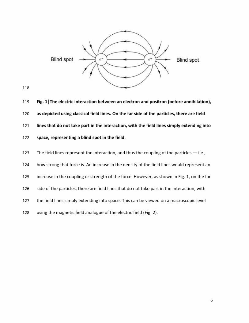
Fig. 1│The electric interaction between an electron and positron (before annihilation), 119
as depicted using classical field lines. On the far side of the particles, there are field 120
lines that do not take part in the interaction, with the field lines simply extending into 121
space, representing a blind spot in the field. 122
The field lines represent the interaction, and thus the coupling of the particles — i.e., 123
how strong that force is. An increase in the density of the field lines would represent an 124
increase in the coupling or strength of the force. However, as shown in Fig. 1, on the far 125
side of the particles, there are field lines that do not take part in the interaction, with 126
the field lines simply extending into space. This can be viewed on a macroscopic level 127
using the magnetic field analogue of the electric field (Fig. 2). 128

7
129
Fig. 2 Shown is a depiction of the magnetic field analogue of the electric field. The 130
drawing shows how iron filings arrange themselves around a magnetic due to the 131
influence of the magnetic field lines. The iron filings effectively map the field lines, 132
showing the blind spot in the field at a macroscopic level, where the field lines in the 133
middle of the far sides of the magnet extend into space with no involvement in the 134
interaction between the magnetic poles. 135
These non-participating field lines exist in a sort of blind spot in the field. This physical 136
condition, by its very nature, affects the coupling of the electrons, as not all field lines 137
are participating in their interaction. It was hypothesized that the blind spot in the 138
electric field affects the numerical value of α. 139
If the field surrounding each particle were divided into an odd number of sectors, the 140
non-participating field lines in the blind spot could be relegated to a single region within 141

8
the larger field, with an equal portion of the electric field on either side of it. Dividing 142
the field into 3 sectors would be the minimum needed for this purpose, but with this, 143
the blind spot would have to take up nearly a third of the electric field, likely 144
overcompensating for the area. Whatever the best value happens to be, there is also 145
the question of whether it should be considered an ad hoc construct or whether the 146
division is something fundamental to the electric field. Only the latter would be of 147
benefit in understanding the nature of α. 148
To help identify an appropriate value to segregate the field lines in the blind spot from 149
the rest of the field, the degrees around the circular field of an unperturbed electron 150
were used. Starting on the far side at the 180-degree mark, in the center of the blind 151
spot, and moving incrementally in 1-degree steps on each side of that mark, fractions of 152
360 degrees were identified that resulted in a whole odd number in the denominator 153
(Fig. 3). As shown in Fig. 3, five numbers (3, 5, 9, 15, 45) were identified up to a span of 154
120 degrees for the whole blind spot (60 degrees on either side of the center). 155
156

9
157
2360 4360
6360 8360 … 24360 … 40360 … 72360 … 120360 158
↓ ↓ ↓ ↓ ↓ ↓ ↓ ↓ 159
1180 190
160 145 115
19 15
13 160
Fig. 3│Division of the electric field into an odd number of sectors, to relegate the blind 161
spot in the field to one sector. Starting on the far side at the 180-degree mark of the 162
field, in the center of the blind spot, and moving incrementally in 1-degree steps on 163
each side of that mark, fractions of 360 degrees were identified that resulted in a 164
whole odd number in the denominator. Five numbers (3, 5, 9, 15, 45) were identified 165
up to a span of 120 degrees for the blind spot (60 degrees on either side of the center). 166
A choice of 9 sectors appears, at least superficially, to be appropriate for several 167
reasons: 1) As noted above, a choice of 3 sectors would be the minimum needed but 168
would overcompensate for the blind spot—which would have to take up a third of the 169
field. Nine is the first multiple of 3 within the identified set and leads to a reasonable 170
size for the blind spot, at a little more than a tenth of the field (1/9). 171
10
With 5 sectors, the blind spot would have to take up nearly a quarter of the electric 172
field. Thus, similar to 3, it would likely overcompensate for the area. The values of 15 173
and 45 would relegate the blind spot to only about 7% and 2% of the field, respectively, 174
likely falling short of the area. Indeed, within the identified set, 9 falls exactly in the 175
middle of the two numbers that would likely overcompensate for the area, and the two 176
that would likely fall short of the area. 177
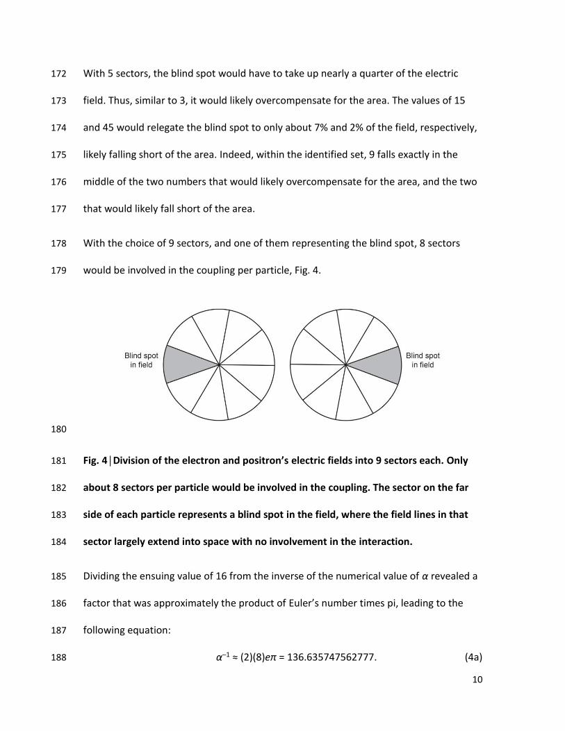
With the choice of 9 sectors, and one of them representing the blind spot, 8 sectors 178
would be involved in the coupling per particle, Fig. 4. 179
180
Fig. 4│Division of the electron and positron’s electric fields into 9 sectors each. Only 181
about 8 sectors per particle would be involved in the coupling. The sector on the far 182
side of each particle represents a blind spot in the field, where the field lines in that 183
sector largely extend into space with no involvement in the interaction. 184
Dividing the ensuing value of 16 from the inverse of the numerical value of α revealed a 185
factor that was approximately the product of Euler’s number times pi, leading to the 186
following equation: 187
α–1 ≈ (2)(8)eπ = 136.635747562777. (4a) 188

11
The fact that two mathematical constants (to an approximation) naturally arose from 189
the choice of 9 (and ultimately 8) sectors per particle also supported the use of 9 for the 190
number of electric field sectors surrounding the particles. 191
However, although the equation produces a result close to the value of α, it does not 192
lead to a match with the 2018 CODATA value of the constant (α–1 = 137.035999084[21]). 193
It is unlikely, however, that the division of the field would be so precise that exactly 8 194
sectors — no more, no less — would be involved in the coupling per particle upon 195
elimination of the blind spot in the field. Rather, it is more likely the case that the sector 196
value would be 8 plus or minus some small amount, likely due, at least in part, to the 197
quantum fluctuations in the overall electromagnetic field, which would alter any 198
geometric precision. 199
Working backward from the currently accepted value of α, the electric field sector value 200
for each particle would be approximately 8.02343465913, such that equation (4a) can 201
be recast as follows: 202
α–1 = (2)(8.02343465913)eπ. (4b) 203
204
205
The amount in excess of 8 — at 0.0234346591350 — is here referred to as the 206
anomalous electric field sector value, a correction needed on the value of 8, just as the 207
anomalous magnetic moment value of 0.00231930436182 is needed on the value of 2 208
for ge. Indeed, the value of the corrective term needed for the sector value is nearly the 209
same as that needed for ge, mostly differing by a simple factor of 10. Here, the electric 210
12
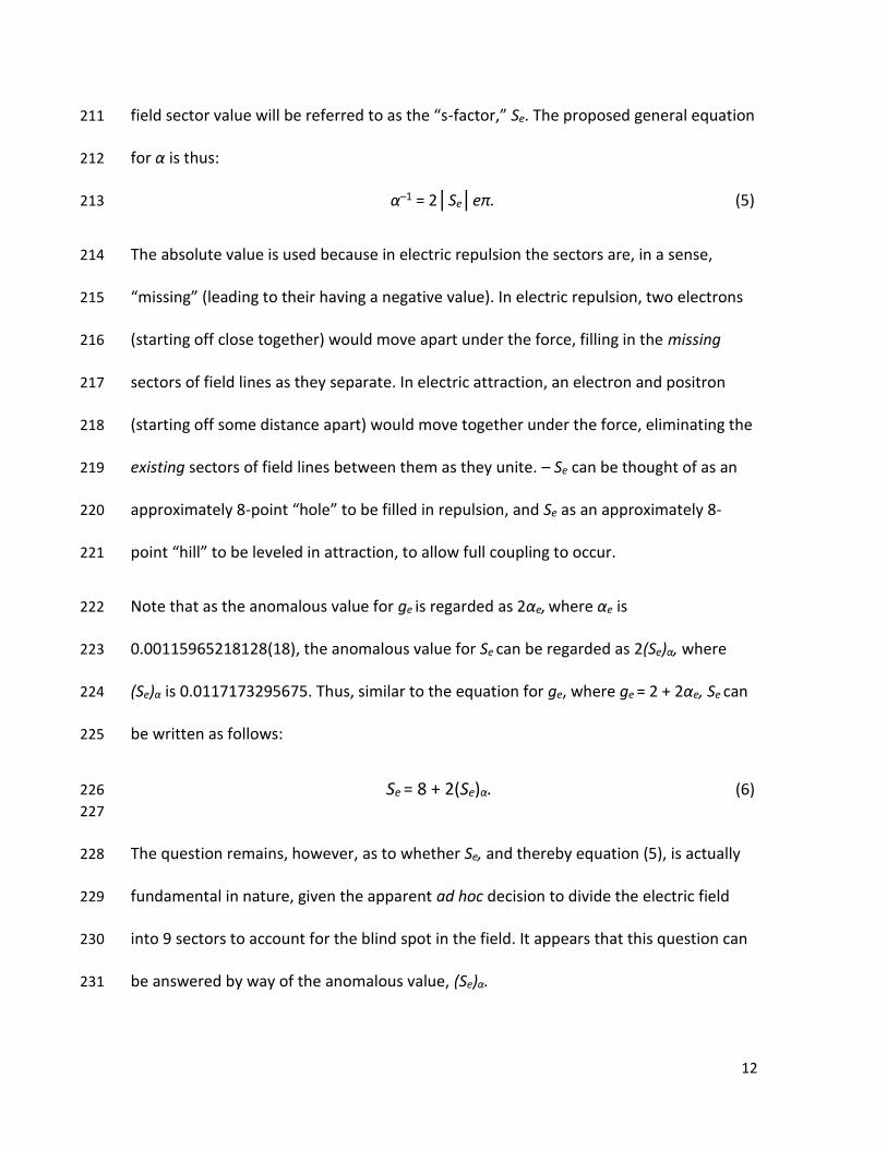
field sector value will be referred to as the “s-factor,” Se. The proposed general equation 211
for α is thus: 212
α–1 = 2│Se│eπ. (5) 213
The absolute value is used because in electric repulsion the sectors are, in a sense, 214
“missing” (leading to their having a negative value). In electric repulsion, two electrons 215
(starting off close together) would move apart under the force, filling in the missing 216
sectors of field lines as they separate. In electric attraction, an electron and positron 217
(starting off some distance apart) would move together under the force, eliminating the 218
existing sectors of field lines between them as they unite. – Se can be thought of as an 219
approximately 8-point “hole” to be filled in repulsion, and Se as an approximately 8-220
point “hill” to be leveled in attraction, to allow full coupling to occur. 221
Note that as the anomalous value for ge is regarded as 2αe, where αe is 222
0.00115965218128(18), the anomalous value for Se can be regarded as 2(Se)α, where 223
(Se)α is 0.0117173295675. Thus, similar to the equation for ge, where ge = 2 + 2αe, Se can 224
be written as follows: 225
Se = 8 + 2(Se)α. (6) 226
227
The question remains, however, as to whether Se, and thereby equation (5), is actually 228
fundamental in nature, given the apparent ad hoc decision to divide the electric field 229
into 9 sectors to account for the blind spot in the field. It appears that this question can 230
be answered by way of the anomalous value, (Se)α. 231

13
As the value of Se is regarded above as a completely arbitrary choice into which to divide 232
the electric field, (Se)α would be an equally arbitrary value, as it directly stems from that 233
choice. As such, it would be highly improbable for (Se)α to have any connection to 234
fundamental constants in nature, being much more likely to have nothing to do with 235
them. However, (Se)α can be derived, to several significant digits, by using the values of 236
the anomalous magnetic moments of the electron, muon, and tau particle (αe, αμ, and 237
ατ, respectively). The result is achieved through the following power series: 238
(𝑆𝑒)𝛼10 ≈ 𝐶0(𝛼𝑒+ 𝛼µ+ 𝛼𝜏)0+ 𝐶1(𝛼𝑒+ 𝛼µ+ 𝛼𝜏)+ 𝐶2(𝛼𝑒+ 𝛼µ+ 𝛼𝜏)2+ …3 (7) 239
where 240
αe = 0.00115965218128(18) 241
αµ = 0.00116592061(41) (From reference 7) 242
ατ = 0.001177171(39) (From reference 8) 243
C0 = 0 244
C1 = 1 245
C2 = 1 + 10(αe) = 1.0115965218128 246
C3 = 1 + 10(αµ) = 1.0116592061 247
C4 = 1 + 10(ατ) = 1.01177171 248
C5 = 1 + ??? ≈ 1.0118… 249
C6 = 1 + ??? ≈ 1.0119… 250
⁞ 251
252
If pattern holds
14
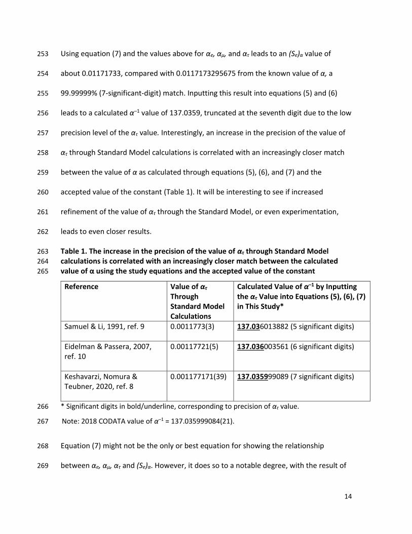
Using equation (7) and the values above for αe, αμ, and ατ leads to an (Se)α value of 253
about 0.01171733, compared with 0.0117173295675 from the known value of α, a 254
99.99999% (7-significant-digit) match. Inputting this result into equations (5) and (6) 255
leads to a calculated α–1 value of 137.0359, truncated at the seventh digit due to the low 256
precision level of the ατ value. Interestingly, an increase in the precision of the value of 257
ατ through Standard Model calculations is correlated with an increasingly closer match 258
between the value of α as calculated through equations (5), (6), and (7) and the 259
accepted value of the constant (Table 1). It will be interesting to see if increased 260
refinement of the value of ατ through the Standard Model, or even experimentation, 261
leads to even closer results. 262
Table 1. The increase in the precision of the value of ατ through Standard Model 263
calculations is correlated with an increasingly closer match between the calculated 264
value of α using the study equations and the accepted value of the constant 265
Reference Value of ατ
Through
Standard Model
Calculations
Calculated Value of α–1 by Inputting
the ατ Value into Equations (5), (6), (7)
in This Study*
Samuel & Li, 1991, ref. 9 0.0011773(3) 137.036013882 (5 significant digits)
Eidelman & Passera, 2007,
ref. 10
0.00117721(5) 137.036003561 (6 significant digits)
Keshavarzi, Nomura &
Teubner, 2020, ref. 8
0.001177171(39) 137.035999089 (7 significant digits)
* Significant digits in bold/underline, corresponding to precision of ατ value. 266
Note: 2018 CODATA value of α–1 = 137.035999084(21). 267
Equation (7) might not be the only or best equation for showing the relationship 268
between αe, αμ, ατ and (Se)α. However, it does so to a notable degree, with the result of 269

15
the expression ultimately leading to a good approximation of the value of α that has 270
only increased in precision as the precision of the value of ατ has increased through 271
Standard Model calculations — with 7 digits of the value of α matched currently. 272
Of course, if future evaluations of αe, αμ, and ατ lead to an exact match with the value of 273
α through equation (7), this would greatly support the idea of a relationship among the 274
magnetic moment anomalies and (Se)α. However, failure to lead to a result beyond a 7-, 275
8-, or 9-digit match with the value of α could also mean the above equation represents 276
only a limiting case of such a relationship or that an adjustment to the formula is 277
needed. Additional support would come from how well the above information 278
intersects with other areas of physics. For example, as shown in section 2.2 below, the 279
value of Se, including its (Se)α component, can also be formulated in a way that is 280
reflective of the quantum electrodynamics (QED) formula for ge, including its αe 281
component. This is also the case for gμ and gτ and their anomalous components. This 282
moderate intersection with QED further suggests there being some degree of a true 283
mathematical relationship between the magnetic moment anomalies and (Se)α. 284
As a value stemming from the completely arbitrary decision to divide the electric field 285
into 9 sectors, having nothing to do with lepton magnetic moment anomalies, there is 286
no a priori reason for (Se)α to have any connection with αe, αμ,,or ατ, unless there is 287
indeed a preexisting natural relationship among them. Such a link would be highly 288
improbable as a random occurrence, as completely fabricated numbers cannot typically 289
be applied in mathematical analyses in any useful way alongside true physical constants 290
with which they had no original connection. 291
16
This suggests that like the values of αe, αμ, and ατ, the value of (Se)α is indeed a real and 292
natural quantity — an anomalous value associated with the electric field of the electron, 293
muon, and tau particle that is mathematically linked to the anomalous values associated 294
with their magnetic fields, as perhaps another example of how electric and magnetic 295
phenomena are linked. This, in turn, would make the value of Se, at approximately 8, 296
also a natural feature of the electric field, and thereby equation (5) a fundamental 297
equation for α. 298
Se being a natural value would mean that, similar to the way that the valence shell of 299
atomic nuclei of the main group elements has 8 zones by which the nuclei interact with 300
electrons, there would be 8 zones or sectors in the space surrounding a lepton by which 301
the particle would engage in coupling with another lepton. The main difference is that 302
the lepton, as a single elementary particle, would be interacting with just one other 303
particle, whereas the sectors surrounding an atomic nucleus, which is composed of 304
multiple protons (themselves composed of multiple elementary particles), would be 305
engaged in interactions with multiple (up to 8) electrons. The atom would be in the 306
most energetically stable state when all 8 of the sectors in its valence shell are engaged 307
in interactions with electrons. Similarly, a lepton would be in the most energetically 308
stable state from the standpoint of electromagnetic coupling when all 8 of its field 309
sectors are engaged in the interaction with the other lepton. Thus, there appears to be a 310
certain symmetry between leptons and atoms, with each being surrounded by 8 distinct 311
sectors of space through which interactions occur. 312

17
Such spatial organization around an electron is not incompatible with the virtual photon 313
cloud concept. Compagno and colleagues noted that it is possible “…to speak of a cloud 314
of virtual photons [surrounding an electron] having a well defined spatial structure” and 315
that generally it is also possible “…to connect some properties of the spatial structure of 316
clouds to the internal dynamics of the source” [11]. In their study of the cloud of virtual 317
photons associated with the hydrogen atom, Passante and colleagues noted that they 318
were “… led to the conclusion that the structure of the virtual cloud of photons in the 319
ground state is in fact an ‘inside-out’ mapping of the electronic structure of the 320
hydrogen atom” [12]. 321
In contrast to the hydrogen atom, elementary particles such as the electron are 322
considered to be point particles, with no internal structure. However, this is a 323
mathematical abstraction, used in large part because of current technological 324
limitations in probing to sizes that would reveal any internal structure. As such, just as it 325
is suggested that the virtual photon cloud associated with the ground state of the 326
hydrogen atom is an “inside-out” mapping of the electronic structure of the atom, so 327
too might the 8-sector electric field, or equivalent virtual photon cloud, of the electron 328
be an “inside-out” mapping of some finer, as yet identified, electronic structure of the 329
elementary particle. Indeed, the identification of the 8 sectors of the electric field might 330
be a first glimpse into that structure. 331
The question of “Why does nature chose 8 specifically?” cannot be immediately 332
answered for either the lepton or the atom. However, this concept would represent yet 333
another “octet rule” in particle physics: In the model above, a lepton couples with 334

18
another lepton through 8 electric field sectors (plus the field’s anomalous portion). The 335
“Eightfold Way” concerns the organization of hadrons, and the currently established 336
“Octet Rule” concerns the 8-zoned valence shell of at least the main group elements, 337
even when there are many more electrons between the nucleus and the valence shell. 338
Thus, while there are always exceptions, a “theme of 8” appears to be carried through 339
from leptons, to hadrons, to some lepton-hadron interactions. 340
Although a quantum mechanical analysis would be needed for further evaluation, there 341
are, thus, several clues that the space surrounding an electron does indeed have a 342
discrete, 8-zoned structure, analogous to the valence shell of many atomic nuclei. The 343
most notable support for this concept comes from the fact that the 8-sector model gives 344
rise to the value of (Se)α, which in turn can be derived to several significant digits from 345
the values of the lepton magnetic moment anomalies, which have been established 346
through theory and/or experimentation. Thus, as the magnetic moment anomalies are 347
true physical quantities, so too are likely the values of (Se)α and Se, which directly stem 348
from them. 349
Therefore, (Se)α and Se appear to be real, nontrivial components in the mathematics of 350
α. In the following sections, this is explored further, and it is shown how the concepts of 351
(Se)α and Se help to explain additional electromagnetic phenomenon and provide even 352
greater clarity regarding the mathematical and physical origins of α. 353
2.1 Types of α Values 354

19
If all 18 sectors were involved between the two interacting particles, α–1 would equal 355
about 153 (from 18eπ) instead of about 137 (from 16eπ)—indeed, at a superficial level, 356
153 seems as “unusual” a number as 137. The different scenarios lead to three types of 357
α values, a basic value (αB) associated with the value 18, encompassing each interacting 358
particle’s full electric field; the true, corrected value of α; and a reduced value (αR) that 359
takes the blind spot per field into account but at a gross level (Table 2). 360
Table 2. Suggested types of the fine-structure constant, α, presented as inverse values 361
Type Symbol Expression Value
Basic value αB–1 18eπ 153.715216008
True (corrected) value α–1 16.046869325eπ 137.035999084*
Reduced (uncorrected) value αR–1 16eπ 136.635747562
*2018 CODATA value. 362
The basic value could not really exist, as it would be physically impossible for all 18 363
sectors to be involved in the coupling in any meaningful way. For this to happen, the 364
field would have to be highly contorted to allow the sectors of field lines on the far side 365
of each particle to play a part in the interaction. 366
As the particles move closer to one another under the electric force of attraction, the 367
field lines involved in the interaction would extend over fewer and fewer sectors of 368
space. Ultimately, there would be zero sectors of space between the particles, and the 369
field line density (number of field lines per sector) would become infinite. As a 370
consequence, the coupling strength would become infinite. This is in accordance with 371

20
the Landau pole — the state of infinite coupling strength in quantum theory, and in this 372
work is represented as follows: 373
374
α–1 = 2│0│eπ = 0; α = ∞. (8) 375
376
377
Thus, the sector value serves as a proxy for field line density, but in the reverse — 378
meaning a decrease in the sector value (as an absolute value) corresponds to an 379
increase in field line density: 380
381
Field line density = Number of field lines│Sector value│ . (9) 382
383
384
Thus, as noted above, the sectors represent a threshold, or barrier, that must be 385
surmounted for full, or infinite, coupling to occur. The greater the sector value, the 386
more substantial the barrier will be and the lower the field line density, and 387
consequently, the lower the coupling strength. 388
The sector value concept can also help explain the change in the value of α at rising 389
energy levels when particles are driven together during collider experiments. That is, the 390
value 1/137 is the approximate value of α at low energy. The constant is said to “run,” 391
or change, as the particles’ energy level changes. When the particles are given higher 392
energy in the collider, the value of α has been measured to rise. At 90 GeV, α has been 393
measured to have a value of approximately 1/128.5 (or 0.007812) [13]. This is the 394
identical value attained when one electric field sector (or its equivalent) is lost in 395

21
equation (5): α–1 = (16.0468693182699 – 1)eπ. Upon collision, each particle’s field would 396
“infiltrate” the other’s, with the effective loss of one sector between them. 397
In electric attraction, the sector value starts off as positive, and an increase in coupling 398
can be viewed as a decrease in this value as the particles move closer together. In 399
electric repulsion, the sector value starts off as negative, and an increase in coupling can 400
be viewed as an increase in this value as the particles move further apart. 401
402
α–1 = 2│8.0234346591350 – x│eπ, (10) 403
(attraction) 404
α–1 = 2│–8.0234346591350 + x│eπ. (11) 405
(repulsion) 406
When enough distance is lost in the setting of electric attraction, or gained in the setting 407
of electric repulsion, to fully mitigate the effects of the sector value, the value would go 408
to zero and the strength of the force would reach infinity. Addition or subtraction 409
beyond zero would have no meaning, as you could not remove more sectors than there 410
are to be removed (in electric attraction) or add more sectors around the particles than 411
can be added (in electric repulsion). 412
2.2 QED-Like Formula for the Anomalous Electric Field Sector Value 413
From a geometric perspective, the anomalous electric field sector value can be divided 414
into 2 subsections: a small amount at the upper end of the blind spot in the electric field 415

22
and an equally small amount at the lower end, due to a natural symmetry around the 416
circular field (Fig. 5). As the full correction in excess of 8 is 0.0234346591350, each 417
subsection, (Se)a, would be half of this, or 0.0117173295675. 418
419
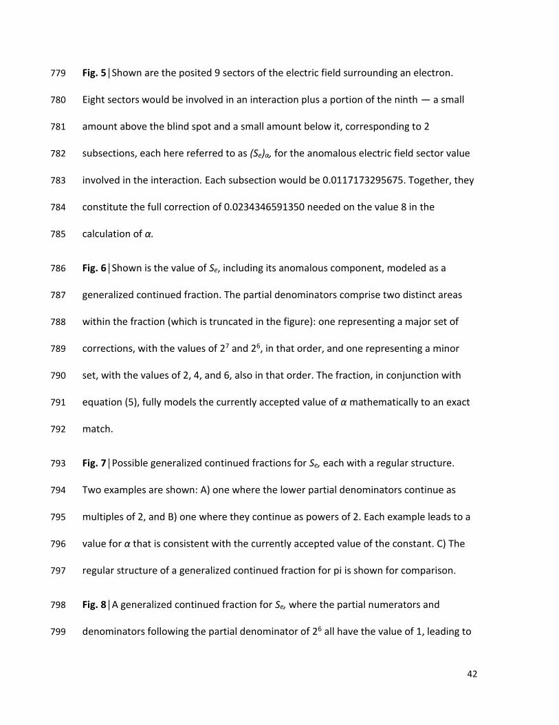
Fig. 5│Shown are the posited 9 sectors of the electric field surrounding an electron. 420
Eight sectors would be involved in an interaction plus a portion of the ninth — a small 421
amount above the blind spot and a small amount below it, corresponding to 2 422
subsections, each here referred to as (Se)α, for the anomalous electric field sector 423
value involved in the interaction. Each subsection would be 0.0117173295675. 424
Together, they constitute the full correction of 0.0234346591350 needed on the value 425
8 in the calculation of α. 426
Thus, as noted above, Se can be written as Se = 8 + 2(Se)α, similar to the equation for ge, 427
where ge = 2 + 2αe. 428
As with the full value of ge, the full value of Se can also be formulated perturbatively. In 429
the case of ge, the perturbative method is applied to quantum field theory, specifically 430
QED. The perturbative formula for the QED contribution to ge is as follows: 431

23
(12) 432
The formal power series of α/π corresponds to quantum corrections as determined 433
through Feynman diagrams, which in turn correspond to real quantum activity at the 434
particle level. The coefficients of the formula (Ci) have been calculated to (α/π)5 and 435
have been confirmed experimentally [6]: 436
C1 = 0.5 C4 = –1.912… 437
C2 = –0.328 … C5 = 6.737…. 438
C3 = 1.181 … 439
The class of quantum activities that would yield a correction on Se is currently not clear. 440
However, Se can be mathematically formulated in a similar way to ge by using αR (again, 441
1/16eπ, see Table 2) in the formal power series in place of α: 442
(13) 443
Using mathematical deduction, several sets of coefficients for equation (13) were 444
identified, each leading to approximately the same value for α when the corresponding 445
Se value was inserted into equation (5). Each solution is also consistent with the 2018 446
CODATA value of the constant (Table 3). 447

24
In each set, the base values of C1 though C5 are the same, at 0.5, 4/π, 3/π, 2/π, and 1/π, 448
respectively, largely following a pattern as multiples of 1/pi. C1 and C2 in each set have 449
exponents of 1. Exponents for C3 through C5 begin with a value of 3 in each set. Starting 450
at C3, the exponents follow a simple numerical sequence in set 1, the prime number 451
sequence in set 2 (which actually can be regarded as beginning with C2), multiples of 3 in 452
set 3, and every fourth number in set 4. Note that each coefficient must be multiplied by 453
a factor of 10 before applying it to equation (13). 454
Table 3. Coefficients for Equation (13), Four Possible Sets* 455
Coefficient Set 1 Set 2 Set 3 Set 4
C1 0.5 0.5 0.5 0.5
C2 4/π 4/π 4/π 4/π
C3 (3/π)3 (3/π)3 (3/π)3 (3/π)3
C4 (2/π)4 (2/π)5 (2/π)6 (2/π)7
C5 (1/π)5 (1/π)7 (1/π)9 (1/π)11
Calculated
α–1 value
137.035999085306… 137.035999084705… 137.035999084323… 137.035999084080…
CODATA α–1 value: 137.035999084(21). 456
*Each coefficient in the table must be multiplied by a factor of 10 before applying to 457
equation (13). 458
459
In the above case, the factor of 10 is considered to be part of the coefficient. Setting 10 460
apart from the coefficients, the equation can be written as follows: 461

25
462 (14) 463
Sets 3 and 4 each appear to lead to the closest match with the current CODATA value, 464
excluding its margins of error. 465
A recent experiment, producing the most precise measurement of α as of 2020, 466
suggests that α–1 might have a value closer to 137.035999206(11) [14]. In this setting, 467
the coefficients could be similar to those listed below, still with a pattern among the 468
values: 469
C1 = 0.5 470
C2 = 4π 471
C3 = √8π 472
C4 = √124 π 473
474
475
C5 = √166 π . 476
These coefficients would lead to an α–1 value of 137.035999217, at the upper end of the 477
experimental value range. 478

26
The perturbative treatments of Se above might serve as purely mathematical formulas. 479
However, given the similarities of the perturbative formulations for ge and Se and the 480
similarity of the anomalous values — at 0.00231930436 for ge and 0.023434659 for Se — 481
the perturbative formulations for Se might be associated with actual physical 482
phenomena at the quantum level, just as the perturbative formulation for ge is. Indeed, 483
as shown above in equation (7), the value of (Se)α appears derivable by using the values 484
of αe, αμ, and ατ, which are themselves derivable through QED. This too supports the 485
idea of (Se)α, and thereby of Se, being associated with actual quantum activity. 486
Note that the ability to identify coefficients by mathematical deduction does not 487
preclude the role of quantum mechanics in nature. For example, the following 488
coefficients, determined by mathematical deduction, could be used in equation (12) for 489
calculating ge: 490
C1 = 0.5 491
C2 = – 13 492
C3 = π23 493
C4 = – π2 494
C5 = 2π2. 495
496

27
They lead to a ge value of 2.00231930436249, a 99.99999999999% (13-significant-digit) 497
match with the 2018 CODATA value of 2.00231930436256(35). QED, however, is one of 498
the most verified physical theories, indicating the existence of actual quantum activity. 499
A better understanding of the quantum activity leading to the anomalous component of 500
Se is needed, perhaps leading to one of the above perturbative formulas or a different 501
one. However, the presented mathematical work does demonstrate that such a 502
formula, linked to actual quantum mechanical phenomena, might be possible. 503
Whether or not a quantum mechanical basis to α is found, it is clear that the constant 504
can be well formulated by using mathematical constants in contrast to what is generally 505
believed today. One of the notable aspects of the formula is its self-consistent nature — 506
that is, αR is the number to be corrected and is, at the same time, the tool by which the 507
correction is attained, as the numerator of the parameter in the power series. 508
Caution should be exercised, however, in attempting to mathematically model whatever 509
the latest CODATA value happens to be. The CODATA value is simply determined 510
through the best experimental studies available at the time it is established, and 511
experimental values have a tendency to shift slightly. Whereas the 2018 CODATA value 512
for α–1 is 137.035999084(21), the 2014 CODATA value was 137.035999139(31), which 513
would require a different set of coefficients than those above. 514
Also, while the above perturbative formulas are characterized by particular patterns 515
among the coefficients, a valid formula for a different experimental value for α might 516

28
not have a pattern (or at least not an obvious one). The principal idea here is that 517
flexibility in any mathematical model is important. 518
If an obvious pattern is detected among the coefficients, and experimental results 519
consistently agree with such a pattern, there is also the possibility that the formula 520
could be used to calculate α to an indefinite number of decimal places, if the expansion 521
diverges. The convergence of such a series would, of course, be invaluable information, 522
as well. 523
In all, the perturbative treatment for Se shown above in conjunction with equation (5) 524
represents, for the first time in history, a full mathematical expression for α that 525
involves mathematical constants, leads to an exact match with the established value of 526
the constant, has the potential to calculate α to an indefinite number of decimal places, 527
and is linked to a physical aspect of the electric field. This physical aspect concerns field 528
geometry at a gross level (accounting for a blind spot in the field), but likely also 529
quantum activity within the greater electromagnetic field. 530
2.3 Alternate Formulas for the Anomalous Electric Field Sector Value 531
As alternate mathematical expressions for calculating a quantity can often be 532
informative, the perturbative solution above was converted into other forms: 1) an 533
alternate perturbative series, with a leading term slightly higher than the value of 4 used 534
above, 2) a related expansion series with non-integer exponents, and 3) a generalized 535
continued fraction. Each offers additional insight into α that might prove useful in 536
further analysis of the constant, both from a mathematical and physical perspective. 537

29
2.3.1.Alternate Perturbative Series and Series Expansion with Non-Integer Exponents 538
In addition to the above, the full value of Se can be formulated as follows: 539
𝑆𝑒2 = 𝐶0𝛼𝑅0 + 𝐶1𝛼𝑅 + 𝐶2𝛼𝑅2 + 𝐶3𝛼𝑅3 + 𝐶4𝛼𝑅4 + 𝐶5𝛼𝑅5 + ⋯, (15) 540
where again, αR is the reduced fine-structure constant (1/16eπ). Given the currently 541
accepted value of α, the following values appear appropriate for the coefficients: 542
543
C0 = 4 + √𝜋3−12 C3 = 𝜋3 544
C1 = 0 C4 = 𝜋7 545
C2 = 1 C5 = 𝜋11. 546
547
Unlike the expression in the previous section, the exactly solvable portion of this 548
expression — that is, the leading term represented by coefficient, C0 — is 4 plus a small 549
amount from an expression involving pi. Such a formula could be important if there is a 550
geometrical aspect to the anomalous value (which the expression after 4 in C0 would 551
likely account for) in addition to quantum activity (which the first through the fifth terms 552
would account for). 553
From C3 onward, the coefficients appear to be a fraction where each numerator is pi and 554
each denominator falls within a linear sequence starting with 3 and then every fourth 555
number thereafter (i.e., 3, 7, 11, …). Increased precision on the 2018 CODATA value 556
would be needed to determine if the pattern remained from C5 onward. When applied 557
to equation (5), the expression leads to a value for α–1 of 137.035999084, an exact, 12-558
significant-digit match with the 2018 CODATA value. 559

30
Equation (15) can also be written as a series expansion with several non-integer 560
exponents: 561
𝑆𝑒2 = 𝐶0𝛼𝑅0 + 𝐶1𝛼𝑅 + 𝐶2𝛼𝑅2 + 𝐶3𝛼𝑅3 + 𝐶4𝛼𝑅4 + (16) 562 𝐶5𝛼𝑅4.001 + 𝐶6𝛼𝑅4.002 + 𝐶7𝛼𝑅4.003 + 563 𝐶8𝛼𝑅4.004 + 𝐶9𝛼𝑅4.005 + 𝐶10𝛼𝑅4.006 …, 564
565
where the coefficients are as follows: 566
C0 = 4 + √𝜋3−12 C3 = 1 C6 = 1 C9 = 1 567
C1 = 0 C4 = 1 C7 = 1 C10 = 1. 568
C2 = 1 C5 = 1 C8 = 1 569
There is a certain “elegant simplicity” to this formula, where all of the coefficients from 570
C2 onward are 1. The 5th through the 10th terms, with exponents of 4.001 through 571
4.006, appear as a subset of the 4th term, with the leading term to the 4th term being 572
the principal portion of the equation. 573
2.3.2. Generalized Continued Fraction 574
Fig. 6 shows the full value of Se modeled as a generalized continued fraction. The 575
number 8 (for the number of principal electric field sectors involved in the coupling) is 576
the leading term of the fraction. The remaining component represents the anomalous 577
value. The partial numerators of the fraction begin with the number 3 and are 1 578
thereafter. The partial denominators comprise two distinct areas within the fraction: 579
one representing a major set of corrections, with the values of 27 and 26, in that order, 580
and one representing a minor set, with the values of 2, 4, and 6, also in that order. The 581

31
major set of corrections alone is associated with an α–1 value of 137.035998746, a 582
99.999999% (8-significant-digit) match with the currently accepted value. The full 583
fraction, of course, leads to the exact value of α. 584
585
α–1 = 2│Se│eπ 586
α–1 = 137.035999084 (via formula) 587
α–1 = 137.035999084(21) (CODATA, 2018) 588
Exact match. 589
Fig. 6│Shown is the value of Se, including its anomalous component, modeled as a 590
generalized continued fraction. The partial denominators comprise two distinct areas 591
within the fraction (which is truncated in the figure): one representing a major set of 592
corrections, with the values of 27 and 26, in that order, and one representing a minor 593
set, with the values of 2, 4, and 6, also in that order. The fraction, in conjunction with 594
equation (5), fully models the currently accepted value of α mathematically to an 595
exact match. 596
Major Set of
Corrections
Minor Set of
Corrections

32
There are several noteworthy issues concerning the fraction, the first of which is its 597
regular structure, providing a straightforward representation of the full value of Se. 598
Indeed, the possibility exists that the fraction has a regular structure that extends 599
indefinitely, as the generalized continued fraction of pi does, although a more precise 600
experimental value of α would be needed to be sure. 601
For example, the partial denominators could continue as multiples of 2 or even powers 602
of 2. Using multiples of 2 and extending the fraction after the partial denominator of 6 603
through a partial denominator of 12 results in an α–1 value of 137.035999084059. 604
Extending the partial denominators as powers of 2, going from 2 through 26, results in 605
an α–1 value of 137.035999083716. Both are consistent with 2018 CODATA value of 606
137.035999084(21) (Fig. 7). 607
608
Extending partial denominators as multiples of 2 leads to an α–1 value of 609
137.035999084059… 610
611

33
612
Extending partial denominators as powers of 2 leads to an α–1 value of 613
137.035999083716… 614
615
616
Pi shown as a generalized continued fraction with a regular structure that extends 617
indefinitely, for comparison. 618
Fig. 7│Possible generalized continued fractions for Se, each with a regular structure. 619
Two examples are shown: A) one where the lower partial denominators continue as 620
multiples of 2, and B) one where they continue as powers of 2. Each example leads to 621

34
a value for α that is consistent with the currently accepted value of the constant. C) 622
The regular structure of a generalized continued fraction for pi is shown for 623
comparison. 624
The generalized continued fraction for Se would be a particularly powerful tool if future 625
evidence suggests that it does indeed have a regular structure throughout. If so, the 626
fraction could be used to determine the value of α to as many decimal places as desired, 627
similar to the potential of the perturbative formulas above. Of course, the possibility 628
also exists that there is no regular structure, or not one beyond the partial 629
denominators of 27 and 26. There is the further possibility that the fraction is finite, with 630
or without a regular structure. 631
As noted above, a recent experiment suggests α–1 might have a value closer to 632
137.035999206(11) [14]. This would be consistent with a generalized continued fraction 633
where all partial numerators and denominators following the partial denominator of 26 634
were a 1, or simply where the remaining fraction after 26 were the inverse of the Golden 635
Ratio, 1.6180339887498948482. In this case, α–1 calculates to a value of approximately 636
137.035999213, which falls within the margin of error of the experimental result (Fig. 8). 637
35
638
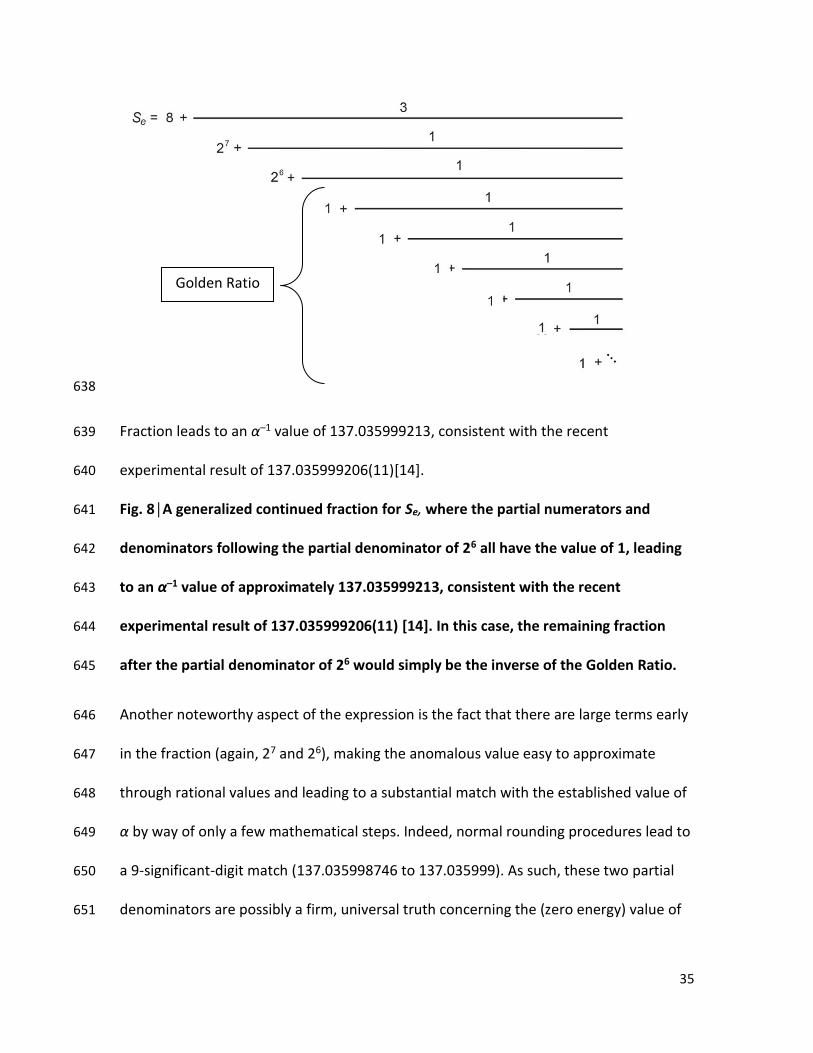
Fraction leads to an α–1 value of 137.035999213, consistent with the recent 639
experimental result of 137.035999206(11)[14]. 640
Fig. 8│A generalized continued fraction for Se, where the partial numerators and 641
denominators following the partial denominator of 26 all have the value of 1, leading 642
to an α–1 value of approximately 137.035999213, consistent with the recent 643
experimental result of 137.035999206(11) [14]. In this case, the remaining fraction 644
after the partial denominator of 26 would simply be the inverse of the Golden Ratio. 645
Another noteworthy aspect of the expression is the fact that there are large terms early 646
in the fraction (again, 27 and 26), making the anomalous value easy to approximate 647
through rational values and leading to a substantial match with the established value of 648
α by way of only a few mathematical steps. Indeed, normal rounding procedures lead to 649
a 9-significant-digit match (137.035998746 to 137.035999). As such, these two partial 650
denominators are possibly a firm, universal truth concerning the (zero energy) value of 651
Golden Ratio

36
the constant. That is, as noted above, experimental results have a tendency to differ 652
slightly. As such, the terms of the fraction that would follow 26 cannot yet be definitively 653
stated. However, many, if not all, agree on at least the first 9 significant digits of the 654
constant’s value, which the first two partial denominators of the generalized continued 655
fraction well lead to. 656
The portion after 26 could be an irrational value, such as the following: 657
Se = 8 + 3______ (17) 658
27 + 1____ 659
26 + √1/5. 660
Although not a traditional generalized continued fraction, this expression also leads to a 661
value for α that is a 12-significant-digit (exact) match with the current CODATA value of 662
the constant. The point here is simply that something “nonclassical” might be happening 663
at a physical level in relation to the area of the fraction following 26 (or a lower point), 664
likely quantum mechanical activity. This would be consistent with the fact that many 665
experiments agree on the first 9 significant digits of α, which again, the portion of the 666
fraction down to 26 will lead to. However, they tend to differ slightly beyond this point. 667
A robust quantum mechanical analysis, if possible, might help to definitively home in on 668
the value of α beyond the first 9 significant digits, and thereby this area of the fraction 669
and which experimental results are likely the most accurate. 670
3. Conclusion 671
37
The nature of α has been a mystery since its discovery more than 100 years ago, and 672
there have been numerous attempts to identify the mathematical basis of the constant. 673
This study presents a full mathematical formula for α that leads to an exact match with 674
the 2018 CODATA value of the constant, and that, importantly, is connected to a 675
physical aspect of the electric field. As such, it is likely connected to quantum 676
mechanical activity also, as the overall electromagnetic field is quantized in nature. 677
At the heart of the mathematics is the idea of a dimensionless anomalous electric field 678
value of about 0.023 associated with the electron. This is particularly notable, as the 679
electron is also associated with a dimensionless anomalous magnetic field value of 680
about 0.023/10, which has been well established through perturbative methods applied 681
to QED and through experimentation. In fact, the anomalous value for the electric field 682
is mathematically linked to the anomalous values of the magnetic fields of each of the 683
charged leptons by way of a simple expression, suggesting that it is a real feature of the 684
electric field, and further suggesting yet another link between electric and magnetic 685
phenomena. 686
Altogether, the concepts introduced here suggest that α is not a random value in the 687
universe, nor does it represent an impenetrable box. Instead, there appear to be 688
accessible mathematics and physics (i.e., quantum activity) inside this box governing the 689
constant and thereby all of the physical phenomena associated with it. This suggests 690
that deeper levels of understanding and discovery might be possible in the setting of the 691
constant. And as α is one of about two dozen dimensionless constants upon which the 692
universe is built, it also suggests that it might be possible to simplify the universe into a 693

38
small set of mathematical constants. The constants might simply need to be arranged in 694
different ways in equations in association with certain physical (perhaps geometrical) 695
conditions of particles and fields, with quantum mechanical activity “filling in the gaps” 696
in terms of attaining accurate and precise results. 697
Of particular note, the transformation of α from an ad hoc value in the Standard Model 698
would serve as a sizeable crack in the ceiling holding the Standard Model back from 699
being a more complete theory of the elementary particles and their interactions. And as 700
α unites fundamental aspects of electromagnetism, quantum physics, and relativity, a 701
deeper understanding of its nature might also assist in efforts to unite the seemingly 702
incompatible physical theories of general relativity and quantum mechanics. 703
4. References 704
1. Tiesinga, E., Mohr, P.J., Newell, D.B. & Taylor, B.N. The 2018 CODATA 705
recommended values of the fundamental physical constants (web version 8.1). 706
Database developed by Baker, J., Douma, M. & Kotochigova, S. Available at 707
http://physics.nist.gov/constants, National Institute of Standards and 708
Technology, Gaithersburg, MD 20899 (2020). 709
2. Dirac, P. A. M. The quantum theory of the electron. Proc. R. Soc. Lond. 710
A 117 (778), 610–624 (1928). 711
3. Aoyama, T., Hayakawa, M., Kinoshita, T. & Nio, M. Tenth-order QED contribution 712
to the electron g − 2 and an improved value of the fine structure constant. Phys. 713
Rev. Lett. 109, 111807 (2012). 714
39
4. Aoyama, T., Hayakawa, M., Kinoshita, T. & Nio, M. Tenth-order electron 715
anomalous magnetic moment — contribution of diagrams without closed lepton 716
loops. Phys. Rev. D 91, 033006 (2015). 717
5. Aoyama, T., Kinoshita, T. & Nio, M. Revised and improved value of the QED 718
tenth-order electron anomalous magnetic moment. Phy. Rev. D 97, 036001 719
(2018). 720
6. Aoyama, T., Kinoshita, T. & Nio, M. Theory of the anomalous magnetic moment 721
of the electron. Atoms 7, 28 (2019). 722
7. Abi, B. et al. (Muon g-2 collaboration). Measurement of the positive muon 723
anomalous magnetic moment to 0.46 ppm. Phy. Rev. Lett. 126, 141801 (2021). 724
8. Keshavarzi, A., Nomura, D. & Teubner, T. g−2 of charged leptons, α(𝑀 2𝑍) and the 725
hyperfine splitting of muonium. Phys. Rev. D 101, 014029 (2020). 726
9. Samuel, M.A. & Li, G. Anomalous magnetic moment of the tau lepton. Phy. Rev. 727
Lett. 67, 668–670 (1991). 728
10. Eidelman, S. & Passera, M. Theory of the tau lepton anomalous magnetic 729
moment. Mod. Phys. Lett. A 22, 159–179 (2007). 730
11. Compagno, G., Passante, R., Persico, F. & Salamone, G.M. Cloud of virtual 731
photons surrounding a nonrelativistic electron. Acta Physica Polonica A 85, 667 – 732
676 (1994). 733
12. Passante, R., Compagno, G. & Persico, F. Cloud of virtual photons in the ground 734
state of the hydrogen atom. Phys. Rev. A 31, 2827–2840 (1985). 735

40
13. Levine, I., Koltick, D., Howell, B. et al. (TOPAZ Collaboration). Measurement of 736
the electromagnetic coupling at large momentum transfer. Phys. Rev. Lett. 78, 737
424–427 (1997). 738
14. Morel, L., Yao, Z., Cladé, P. et al. Determination of the fine-structure constant 739
with an accuracy of 81 parts per trillion. Nature 588, 61–65 (2020). 740
5. Acknowledgement 741
The author extends special thanks to Gary Mark Roberts for the drawings in the 742
manuscript. 743
6. Author Contribution Statement 744
The author provided all written content in the manuscript. 745
7. Additional Information 746
The author declares no competing interests. 747
The author has no relevant financial or non-financial interests to disclose. 748
The author has no conflicts of interest to declare that are relevant to the content of this 749
article. 750
The author certifies that he has no affiliations with or involvement in any organization or 751
entity with any financial interest or non-financial interest in the subject matter or 752
materials discussed in this manuscript. 753
The author has no financial or proprietary interests in any material discussed in this 754
article. 755
The data that support the findings of this study are openly available in the 2018 CODATA 756
Recommended Values of the Fundamental Physical Constants, reference number 1. 757

41
8. Figure Legends 758
Fig. 1│The electric interaction between an electron and positron (before annihilation), 759
as depicted using classical field lines. On the far side of the particles, there are field lines 760
that do not take part in the interaction, with the field lines simply extending into space, 761
representing a blind spot in the field. 762
Fig. 2 Shown is a depiction of the magnetic field analogue of the electric field. The 763
drawing shows how iron filings arrange themselves around a magnetic due to the 764
influence of the magnetic field lines. The iron filings effectively map the field lines, 765
showing the blind spot in the field at a macroscopic level, where the field lines in the 766
middle of the far sides of the magnet extend into space with no involvement in the 767
interaction between the magnetic poles. 768
Fig. 3│Division of the electric field into an odd number of sectors, to relegate the blind 769
spot in the field to one sector. Starting on the far side at the 180-degree mark of the 770
field, in the center of the blind spot, and moving incrementally in 1-degree steps on 771
each side of that mark, fractions of 360 degrees were identified that resulted in a whole 772
odd number in the denominator. Five numbers (3, 5, 9, 15, 45) were identified up to a 773
span of 120 degrees for the blind spot (60 degrees on either side of the center). 774
Fig. 4│Division of the electron and positron’s electric fields into 9 sectors each. Only 775
about 8 sectors per particle would be involved in the coupling. The sector on the far side 776
of each particle represents a blind spot in the field, where the field lines in that sector 777
largely extend into space with no involvement in the interaction. 778
42
Fig. 5│Shown are the posited 9 sectors of the electric field surrounding an electron. 779
Eight sectors would be involved in an interaction plus a portion of the ninth — a small 780
amount above the blind spot and a small amount below it, corresponding to 2 781
subsections, each here referred to as (Se)α, for the anomalous electric field sector value 782
involved in the interaction. Each subsection would be 0.0117173295675. Together, they 783
constitute the full correction of 0.0234346591350 needed on the value 8 in the 784
calculation of α. 785
Fig. 6│Shown is the value of Se, including its anomalous component, modeled as a 786
generalized continued fraction. The partial denominators comprise two distinct areas 787
within the fraction (which is truncated in the figure): one representing a major set of 788
corrections, with the values of 27 and 26, in that order, and one representing a minor 789
set, with the values of 2, 4, and 6, also in that order. The fraction, in conjunction with 790
equation (5), fully models the currently accepted value of α mathematically to an exact 791
match. 792
Fig. 7│Possible generalized continued fractions for Se, each with a regular structure. 793
Two examples are shown: A) one where the lower partial denominators continue as 794
multiples of 2, and B) one where they continue as powers of 2. Each example leads to a 795
value for α that is consistent with the currently accepted value of the constant. C) The 796
regular structure of a generalized continued fraction for pi is shown for comparison. 797
Fig. 8│A generalized continued fraction for Se, where the partial numerators and 798
denominators following the partial denominator of 26 all have the value of 1, leading to 799

43
an α–1 value of approximately 137.035999213, consistent with the recent experimental 800
result of 137.035999206(11) [14]. In this case, the remaining fraction after the partial 801
denominator of 26 would simply be the inverse of the Golden Ratio. 802
9. Tables 803
Table 1. The increase in the precision of the value of ατ through Standard Model 804
calculations is correlated with an increasingly closer match between the calculated 805
value of α using the study equations and the accepted value of the constant 806
Reference Value of ατ
Through
Standard Model
Calculations
Calculated Value of α–1 by Inputting
the ατ Value into Equations (5), (6), (7)
in This Study*
Samuel & Li, 1991, ref. 9 0.0011773(3) 137.036013882 (5 significant digits)
Eidelman & Passera, 2007,
ref. 10
0.00117721(5) 137.036003561 (6 significant digits)
Keshavarzi, Nomura &
Teubner, 2020, ref. 8
0.001177171(39) 137.035999089 (7 significant digits)
* Significant digits in bold/underline, corresponding to precision of ατ value. 807
Note: 2018 CODATA value of α–1 = 137.035999084(21). 808
Table 2. Suggested types of the fine-structure constant, α, presented as inverse values 809
Type Symbol Equation Value
Basic value αB–1 18eπ 153.715216008
True (Corrected) value α–1 16.046869325eπ 137.035999084*
Reduced (Uncorrected) value αR–1 16eπ 136.635747562
*2018 CODATA value. 810
811

44
Table 3. Coefficients for Equation (13), Four Possible Sets* 812
Coefficient Set 1 Set 2 Set 3 Set 4
C1 0.5 0.5 0.5 0.5
C2 4/π 4/π 4/π 4/π
C3 (3/π)3 (3/π)3 (3/π)3 (3/π)3
C4 (2/π)4 (2/π)5 (2/π)6 (2/π)7
C5 (1/π)5 (1/π)7 (1/π)9 (1/π)11
Calculated
α–1 value
137.035999085306… 137.035999084705… 137.035999084323… 137.035999084080…
CODATA α–1 value: 137.035999084(21). 813
*Each coefficient in the table must be multiplied by a factor of 10 before applying to 814
equation (13). 815
816