AN INVESTIGATION OF THE PHYSICAL PROPERTIES OF …

AFRL-RV-PS- AFRL-RV-PS- TR-2014-0195 TR-2014-0195 AN INVESTIGATION OF THE PHYSICAL PROPERTIES OF ERUPTING SOLAR PROMINENCES, PHASE II Richard C. Altrock, et al. 30 December 2014 Final Report

APPROVED FOR PUBLIC RELEASE; DISTRIBUTION IS UNLIMITED.

AIR FORCE RESEARCH LABORATORY Space Vehicles Directorate 3550 Aberdeen Ave SE AIR FORCE MATERIEL COMMAND KIRTLAND AIR FORCE BASE, NM 87117-5776

NOTICE AND SIGNATURE PAGE

Using Government drawings, specifications, or other data included in this document for any purpose other than Government procurement does not in any way obligate the U.S. Government. The fact that the Government formulated or supplied the drawings, specifications, or other data does not license the holder or any other person or corporation; or convey any rights or permission to manufacture, use, or sell any patented invention that may relate to them.

This report was cleared for public release by the 377 ABW Public Affairs Office and is available to the general public, including foreign nationals. Copies may be obtained from the Defense Technical Information Center (DTIC) (http://www.dtic.mil).

AFRL-RV-PS-TR-2014-0195 HAS BEEN REVIEWED AND IS APPROVED FOR PUBLICATION IN ACCORDANCE WITH ASSIGNED DISTRIBUTION STATEMENT.

//SIGNED// //SIGNED// _____________________________________ _______________________________________ Dr. Richard C. Altrock Glenn M. Vaughan, Colonel, USAF Project Manager, AFRL/RVBXS Chief, Battlespace Environment Division

DTIC COPY

This report is published in the interest of scientific and technical information exchange, and its publication does not constitute the Government’s approval or disapproval of its ideas or findings.

Approved for Public Release; Distribution is Unlimited.

REPORT DOCUMENTATION PAGE Form Approved

OMB No. 0704-0188 Public reporting burden for this collection of information is estimated to average 1 hour per response, including the time for reviewing instructions, searching existing data sources, gathering and maintaining the data needed, and completing and reviewing this collection of information. Send comments regarding this burden estimate or any other aspect of this collection of information, including suggestions for reducing this burden to Department of Defense, Washington Headquarters Services, Directorate for Information Operations and Reports (0704-0188), 1215 Jefferson Davis Highway, Suite 1204, Arlington, VA 22202-4302. Respondents should be aware that notwithstanding any other provision of law, no person shall be subject to any penalty for failing to comply with a collection of information if it does not display a currently valid OMB control number. PLEASE DO NOT RETURN YOUR FORM TO THE ABOVE ADDRESS. 1. REPORT DATE (DD-MM-YYYY)30-12-2014

2. REPORT TYPEFinal Report

3. DATES COVERED (From - To)21 Mar 2011 to 30 Dec 2014

4. TITLE AND SUBTITLEAn Investigation of the Physical Properties of Erupting Solar Prominences, Phase II

5a. CONTRACT NUMBER

5b. GRANT NUMBER

5c. PROGRAM ELEMENT NUMBER 61102F

6. AUTHOR(S)Richard C. Altrock, J. Lewis Fox1, and Roberto Casini2

5d. PROJECT NUMBER 3001

5e. TASK NUMBER PPM00012251

5f. WORK UNIT NUMBEREF004374

7. PERFORMING ORGANIZATION NAME(S) AND ADDRESS(ES)Air Force Research Laboratory 1National Solar Observatory 2High Altitude ObservatorySpace Vehicles Directorate PO Box 62 PO Box 3000 3550 Aberdeen Avenue SE Sunspot, NM 88349 Boulder, CO 80307 Kirtland AFB, NM 87117-5776

8. PERFORMING ORGANIZATION REPORTNUMBER

AFRL-RV-PS-TR-2014-0195

9. SPONSORING / MONITORING AGENCY NAME(S) AND ADDRESS(ES) 10. SPONSOR/MONITOR’S ACRONYM(S)AFRL/RVBXS

11. SPONSOR/MONITOR’S REPORTNUMBER(S)

12. DISTRIBUTION / AVAILABILITY STATEMENT

Approved for Public Release; Distribution is Unlimited. (377ABW-2015-0291 dtd 6 Apr 2015)

13. SUPPLEMENTARY NOTES

14. ABSTRACTThe Prominence Magnetometer (ProMag) is a dual-channel, dual-beam spectro-polarimeter designed by the High Altitude Observatory at the National Center for Atmospheric Research (HAO/NCAR) for the study of the magnetism of solar prominences and filaments with the ultimate goal of predicting prominence activation and eruptions. It was deployed in August 2009 at the 40-cm coronagraph of the Evans Solar Facility (ESF) of the National Solar Observatory on Sacramento Peak (NSO/SP). For two years HAO staff operated the instrument in “campaign mode”, in which a two week observing campaign ran once per quarter. The Air Force Office of Scientific Research funded a three-year program to run the instrument in “synoptic mode”, in which data is taken daily on many prominences. In this report we summarize progress towards the goals of this three-year program. Dr. J. Lewis Fox became the ProMag Observing Scientist in residence at Sacramento Peak, August 2011 as a postdoctoral research associate funded through the AFOSR program and employed by the National Solar Observatory. Since that time Dr. Fox has completed a redesign of the instrument. Data reduction software, including polarimetric calibration is now nearly complete. He has carried out two years of routine observations, resulting in the observation of hundreds of prominences and filaments and trained two observers to carry out ProMag observations independently.

15. SUBJECT TERMSSolar prominences, Solar prominence eruption, Solar coronal mass ejection, Solar activity, Solar instrumentation 16. SECURITY CLASSIFICATION OF: 17. LIMITATION

OF ABSTRACT 18. NUMBEROF PAGES

19a. NAME OF RESPONSIBLE PERSONDr. Richard C. Altrock

a. REPORTUnclassified

b. ABSTRACTUnclassified

c. THIS PAGEUnclassified Unlimited

19b. TELEPHONE NUMBER (include area code)

Standard Form 298 (Rev. 8-98) Prescribed by ANSI Std. 239.18

48

AFOSR Task 11RV01COR

Final Report AFOSR Task 11RV01COR

This page is intentionally left blank.


Table of Contents

1. INTRODUCTION .....................................................................................................................1

2. BACKGROUND .......................................................................................................................1

3. METHODS, ASSUMPTIONS, AND PROCEDURES .............................................................2

3.1 Current Design ...................................................................................................................2 3.2 Motivation for Modification ..............................................................................................7

3.3 Future Design Modifications .............................................................................................9

3.4 Comsequences of the Design Change ...............................................................................9

3.4.1 Modulation Efficiency .............................................................................................9

3.4.2 Telescope Calibration ............................................................................................10

3.4.3 Focus ......................................................................................................................11

3.5 Calibration........................................................................................................................13

3.6 Observation Sequence ......................................................................................................14

4. RESULTS AND DISCUSSION ..............................................................................................15

4.1 Calibration Results ...........................................................................................................23

4.2 Time Variability of the Extended Modulator ..................................................................24

4.3 Stability Analysis .............................................................................................................26

4.4 Flat Fielding .....................................................................................................................32

5. CONCLUSIONS.....................................................................................................................35

6. ACKNOWLEDGEMENTS ....................................................................................................37

REFERENCES .......................................................................................................................38

LIST OF ACRONYMS ..........................................................................................................39

iApproved for Public Release; Distribution is Unlimited.

List of Figures

1. Optical Layout of ProMag at ESF ..............................................................................................3

2. The ProMag Polarimeter .............................................................................................................4

3. Theoretical modulation efficiencies for the design prescription given in Table 1 .....................5

4. Schematic of the image rotator prism .........................................................................................6

5. East bench focus .......................................................................................................................12

6. Total intensity of calibration images.........................................................................................13

7. Gong image from June 18, 2013. The circled prominence is the target ...................................14

8. ProMag data by date and time ..................................................................................................16

9. Prominence map from August 25, 2012 ...................................................................................17

10. Selected scan positions in a prominence from June 18, 2013.................................................17

11. Prominence reconstructions from October 9, 2012 in both D3 (a) and IR (b) .......................18

12. Profiles along the slit, and in the wavelength direction from Oct 9, 2012 .............................19

13. Post-flare loop observation from May 22, 2013 .....................................................................20

14. Line profiles from the May 22, 2013 post-flare loop..............................................................20

15. Succession of map reconstructions for the April 29, 2014 eruptive prominence ...................21

16. Raster from the pre-eruption map, beginning 183621 UTC ...................................................21

17. Rasters from the 1st eruption map, beginning 193505 UTC ..................................................21

18. Rasters from the 2nd eruption map, beginning 203824 UTC .................................................22

19. Rasters from the 3rd eruption map, beginning 212534 UTC .................................................22

20. Raster from the post-eruption map, beginning 222551 UTC .................................................23

21. Calibration clear frame with super-pixel grid .........................................................................23

22. Calibration parameters over time ............................................................................................24

ii Approved for Public Release; Distribution is Unlimited.

List of Figures, continued

23. Calibration Stokes parameters and modulation efficiencies over time ...................................25

24. Calibration modulation matrix over time ................................................................................26

25. χ2 for a calibration set taken April 16, 2013 at 194201 UTC .................................................27

26. Calibration retardance and transmittance................................................................................28

27. Calibration polarizer and retarder offset angles ......................................................................28

28. Stokes IQUV and their associated modulation efficiencies ....................................................29

29. Modulation matrix for April 16, 2013, 194201 UTC .............................................................30

30. Modulation matrix for the 2nd beam ......................................................................................31

31. Sum of the modulation matrices from the two beams ............................................................32

32. Experimental flat field using the Kuhn method ......................................................................33

33. Raw calibration clear vs. flat fielded calibration clear ...........................................................33

34. Raw calibration clear vs. PCA reconstructed calibration clear ...............................................33

35. Comparison of raw calibration set with PCA reconstruction .................................................34

36. Comparison of Stokes parameters between raw and PCA reconstructed sets.........................34

37. Modulation matrix for the raw and PCA reconstruction ........................................................35

iii Approved for Public Release; Distribution is Unlimited.

List of Tables

1. Final ProMag modulator design as implemented.....................................................................5

2. .Modulation efficiencies for ProMag.......................................................................................10

iv Approved for Public Release; Distribution is Unlimited.

1. INTRODUCTION

Note: Much of this report, especially the later Sections, is written for an audience with advanced knowledge of spectro-polarimetric instrument design and analysis techniques. Readers may find it useful to first review Section 5, Conclusions, which is written in a style of an executive summary.

The Prominence Magnetometer (ProMag) is a dual-channel, dual-beam spectro-polarimeter designed by the High Altitude Observatory at the National Center for Atmospheric Research (HAO/NCAR) for the study of the magnetism of solar prominences and filaments with the ultimate goal of predicting prominence activation and eruptions. It was deployed in August 2009 at the 40-cm coronagraph of the Evans Solar Facility (ESF) of the National Solar Observatory on Sacramento Peak (NSO/SP).

For two years HAO staff operated the instrument in “campaign mode”, in which a two week observing campaign ran once per quarter. However, this proved insufficient to truly gain understanding of prominence behavior, which requires much more routine data acquisition. The Air Force Office of Scientific Research funded a three-year program to run the instrument in “synoptic mode”, in which data is taken daily on many prominences. . In this report we summarize progress towards the goals of this three-year program.

Dr. J. Lewis Fox became the ProMag Observing Scientist in residence at Sacramento Peak in August 2011 as a postdoctoral research associate funded through AFOSR and employed by the National Solar Observatory. Since that time Dr. Fox has completed a redesign of the instrument. Data reduction software, including polarimetric calibration is now nearly complete. Observing modes and programs exist for both prominences and filaments. He has carried out two years of routine observations, resulting in the observation of hundreds of prominences and filaments and trained two observers to carry out ProMag observations independently.

2. BACKGROUND

To understand space weather and the Sun-Earth connection it is necessary to measure the full vector magnetic field in the solar corona. Changing magnetic fields in the photosphere, coupled with photospheric convective motions, drive the dynamics and heating of the corona, but the linkages through the chromosphere and transition region, areas of intermediate plasma β and non-potential and/or non-force-free fields, are poorly determined. The large-scale magnetic topology supporting prominences and filaments guides the evolution of these solar structures, which have important, direct consequences for space weather and its effects on terrestrial technology and civilization. For space weather purposes, the ultimate goal of prominence research is the successful prediction of prominence eruptions leading to earth-directed Coronal Mass Ejections (CMEs). We aim to measure the vector magnetic field in prominences and filaments, and do so routinely. While prominence magnetic field measurements have been made successfully at the Dunn Solar Telescope (NSO/SP) [1] and the THÉMIS solar telescope on Tenerife [2], these telescopes have too much scattered light to observe many prominences, and are over-subscribed by the community. With the Prominence Magnetometer (ProMag) operating at the Evans Solar Facility (ESF) coronagraph we have the opportunity to build a “patrol mode” catalog of

1 Approved for Public Release; Distribution is Unlimited.

prominence observations, leading ultimately to a better understanding of prominence behavior and metrics predicting eruption. In ProMag’s standard mode of operation, it acquires spectro-polarimetric maps of solar targets simultaneously in the chromospheric lines of He I at 587.6 nm and 1083.0 nm and in two orthogonal states of polarization. It performs full-Stokes spectro-polarimetry, using Hanlé effect polarization measurements to infer the full vector magnetic field, as well as other physical parameters of the plasma. The key to this capability is simultaneous, co-spectral, co-spatial, high efficiency modulation of the incoming solar beam in one or two spectral channels and in both oppositely-polarized beams. ProMag achieves this with a novel polychromatic integrated modulator/analysis unit designed for high efficiency across a broad spectral band. Because the modulation cycle is slow relative to the turbulence timescale for atmosphere seeing, and the ESF does not have a seeing-correction system, dual-beam polarimetry is an essential feature of the ProMag design, in order to eliminate seeing-induced polarization cross-talk. Since deployment in August 2009, the ProMag instrument has operated in campaign mode, and since August 2011 in patrol mode with a dedicated observer. We have modified the original design in response to a difficulty in aligning the two polarimeter beams on the entrance slit of the spectrograph, which prevented the strict co-spatiality required for these sensitive measurements. We moved the polarimeter modulation and analysis unit from the prime focus of the ESF coronagraph to the spectrograph, downstream of the slit. Observations taken with ProMag are now truly simultaneous, in space, spectrum, and time. The same slit, modulator, and analyzer are used in both beams and both spectral channels. Full instrument realignment, consequent to the configuration change, was completed in July 2012. The prominence observing program with the new instrument commenced in earnest in August 2012. The most significant consequence of the change is a radical alteration in the instrument calibration plan. The new configuration effectively makes the telescope a part of the modulator and produces calibrations which vary on both daily (with telescope hour-angle) and seasonal (with solar declination) time-scales. This has led to a new approach to instrument calibration. In this report we present the ProMag design (§3.1) as currently implemented, the motivation for altering the original design (§3.2), the consequences of the design change (§3.4), and the current calibration procedure (§3.5). We will then discuss the current status of the ProMag observing program and report current progress in performing calibrations.

3. METHODS, ASSUMPTIONS, AND PROCEDURES

The original design is presented in [3], along with a more detailed scientific case, and the instrument requirements derived from typical prominence parameters. This material will not be repeated here, except where changes have taken place. The original design and the deployed design were not identical. Further post-deployment changes to the design were proposed in August 2011. These changes were implemented between December 2011 and July 2012. In this report we document the current design only.

3.1 Current Design

The optical system at the ESF, including ProMag is shown in Figure 1. It includes the telescope’s objective lens (O1) followed by the occulter assembly at prime focus (F1). The F1 assembly


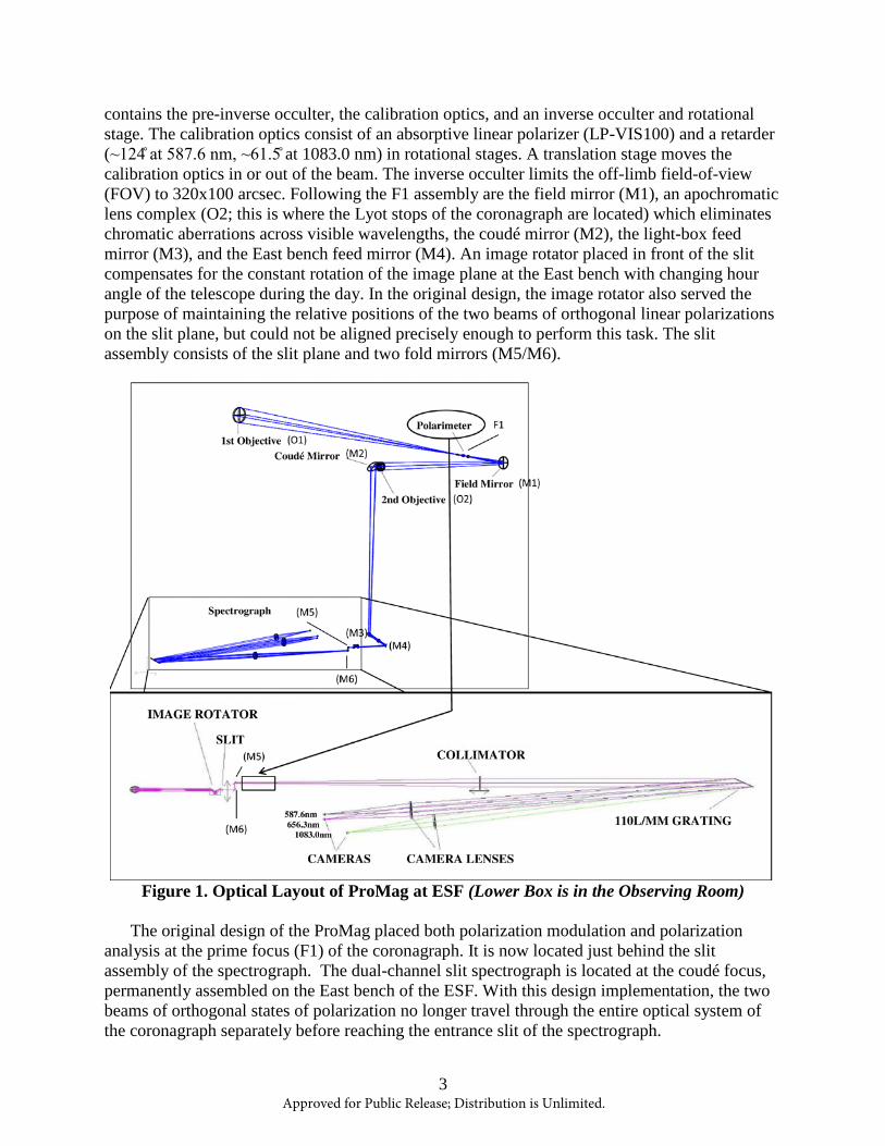
contains the pre-inverse occulter, the calibration optics, and an inverse occulter and rotational stage. The calibration optics consist of an absorptive linear polarizer (LP-VIS100) and a retarder (~124̊ at 587.6 nm, ~61.5̊ at 1083.0 nm) in rotational stages. A translation stage moves the calibration optics in or out of the beam. The inverse occulter limits the off-limb field-of-view (FOV) to 320x100 arcsec. Following the F1 assembly are the field mirror (M1), an apochromatic lens complex (O2; this is where the Lyot stops of the coronagraph are located) which eliminates chromatic aberrations across visible wavelengths, the coudé mirror (M2), the light-box feed mirror (M3), and the East bench feed mirror (M4). An image rotator placed in front of the slit compensates for the constant rotation of the image plane at the East bench with changing hour angle of the telescope during the day. In the original design, the image rotator also served the purpose of maintaining the relative positions of the two beams of orthogonal linear polarizations on the slit plane, but could not be aligned precisely enough to perform this task. The slit assembly consists of the slit plane and two fold mirrors (M5/M6).

Figure 1. Optical Layout of ProMag at ESF (Lower Box is in the Observing Room)

The original design of the ProMag placed both polarization modulation and polarization analysis at the prime focus (F1) of the coronagraph. It is now located just behind the slit assembly of the spectrograph. The dual-channel slit spectrograph is located at the coudé focus, permanently assembled on the East bench of the ESF. With this design implementation, the two beams of orthogonal states of polarization no longer travel through the entire optical system of the coronagraph separately before reaching the entrance slit of the spectrograph.


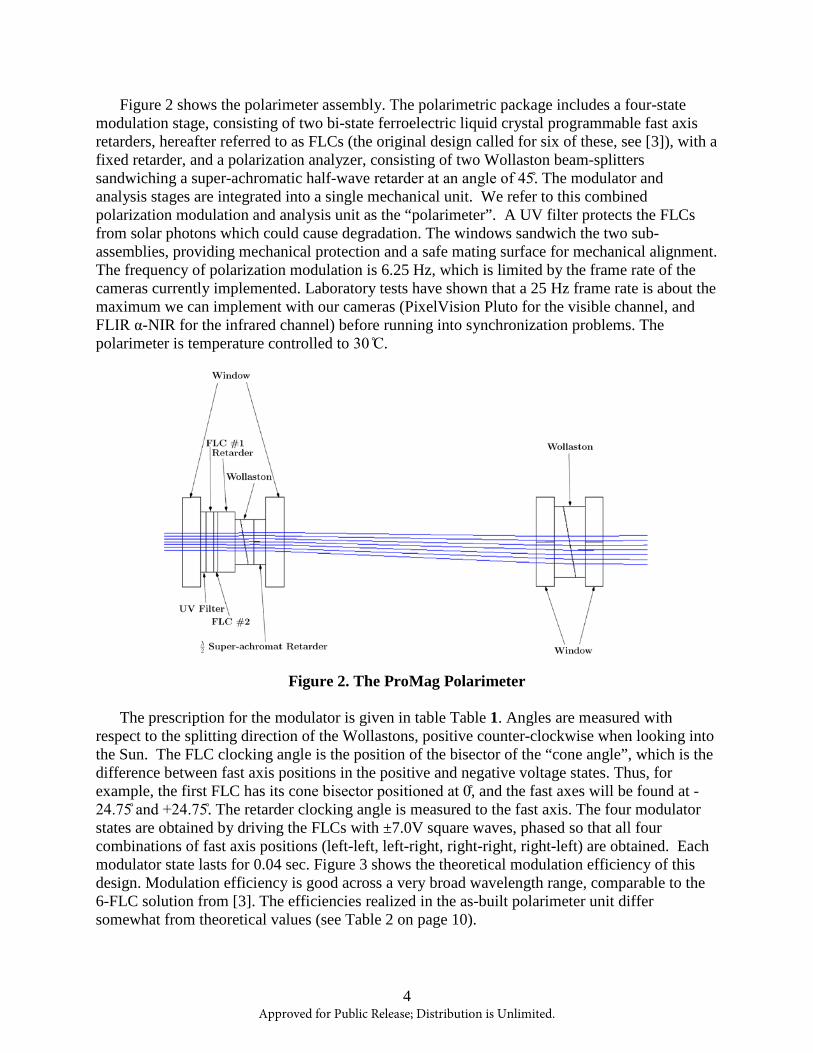
Figure 2 shows the polarimeter assembly. The polarimetric package includes a four-state modulation stage, consisting of two bi-state ferroelectric liquid crystal programmable fast axis retarders, hereafter referred to as FLCs (the original design called for six of these, see [3]), with a fixed retarder, and a polarization analyzer, consisting of two Wollaston beam-splitters sandwiching a super-achromatic half-wave retarder at an angle of 45̊. The modulator and analysis stages are integrated into a single mechanical unit. We refer to this combined polarization modulation and analysis unit as the “polarimeter”. A UV filter protects the FLCs from solar photons which could cause degradation. The windows sandwich the two sub-assemblies, providing mechanical protection and a safe mating surface for mechanical alignment. The frequency of polarization modulation is 6.25 Hz, which is limited by the frame rate of the cameras currently implemented. Laboratory tests have shown that a 25 Hz frame rate is about the maximum we can implement with our cameras (PixelVision Pluto for the visible channel, and FLIR α-NIR for the infrared channel) before running into synchronization problems. The polarimeter is temperature controlled to 30 ̊C.

Figure 2. The ProMag Polarimeter

The prescription for the modulator is given in table Table 1. Angles are measured with respect to the splitting direction of the Wollastons, positive counter-clockwise when looking into the Sun. The FLC clocking angle is the position of the bisector of the “cone angle”, which is the difference between fast axis positions in the positive and negative voltage states. Thus, for example, the first FLC has its cone bisector positioned at 0̊, and the fast axes will be found at -24.75̊ and +24.75̊. The retarder clocking angle is measured to the fast axis. The four modulator states are obtained by driving the FLCs with ±7.0V square waves, phased so that all four combinations of fast axis positions (left-left, left-right, right-right, right-left) are obtained. Each modulator state lasts for 0.04 sec. Figure 3 shows the theoretical modulation efficiency of this design. Modulation efficiency is good across a very broad wavelength range, comparable to the 6-FLC solution from [3]. The efficiencies realized in the as-built polarimeter unit differ somewhat from theoretical values (see Table 2 on page 10).


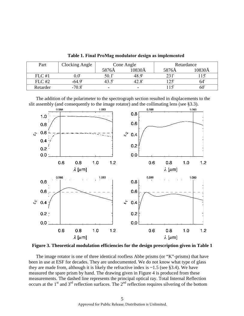
Table 1. Final ProMag modulator design as implemented

Part Clocking Angle Cone Angle Retardance 5876Å 10830Å 5876Å 10830Å

FLC #1 0.0̊ 50.1̊ 48.9̊ 231̊ 115̊ FLC #2 -64.9̊ 43.5̊ 42.8̊ 125̊ 64̊ Retarder -70.8̊ - - 115̊ 60̊

The addition of the polarimeter to the spectrograph section resulted in displacements to the slit assembly (and consequently to the image rotator) and the collimating lens (see §3.3).

Figure 3. Theoretical modulation efficiencies for the design prescription given in Table 1

The image rotator is one of three identical roofless Abbe prisms (or “K”-prisms) that have been in use at ESF for decades. They are undocumented. We do not know what type of glass they are made from, although it is likely the refractive index is ~1.5 (see §3.4). We have measured the spare prism by hand. The drawing given in Figure 4 is produced from these measurements. The dashed line represents the principal optical ray. Total Internal Reflection occurs at the 1st and 3rd reflection surfaces. The 2nd reflection requires silvering of the bottom


surface. The coating material for this surface is unknown, as are the prism glass and the index matching cement used in the interface between the two prism halves. See §3.4 for more details on the effect of this prism on focus.

Figure 4. Schematic of the image rotator prism


3.2 Motivation for Modification

The original polarimetric configuration of the ProMag can be conveniently expressed in terms of a train of Mueller matrices for the system. If I is the input Stokes vector at the entrance of the telescope, then the analyzed signal vector for the two orthogonally-polarized beams as function of time, I±(t), is given by

[1]

where P±M(t) describes the polarization modulation and analysis package for the two beams (+ and -), T(t) accounts for the telescope’s optics (including the image rotator), and S describes the spectrograph (from the collimator lens down). We note that the modulator's Mueller matrix is a function of time due to the changing states of the modulator during a cycle (at the 25 Hz rate), whereas the telescope's Mueller matrix is a function of time due to the changing hour angle of the telescope during an observation and the changing declination angle of the coudé mirror during the year. This temporal variation of the telescope also includes the image rotator, and can be considered a “secular” term with respect to the faster temporal dependence of the polarimeter (the typical duration of a map scan is of the order of 0.5 hr, corresponding to a rotation of the image plane of 7.5̊). We note that we omitted the Mueller matrix of O1 from the expression of eq. [1], since by assumption this is equivalent to the identity matrix (apart from an overall transmission factor). Calibration optics (a linear polarizer and a retarder) are inserted in the beam for polarization calibration. These optics may be described by a (variable) Mueller matrix C that precedes M(t) in eq. [1]. The polarization modulation and analysis was originally performed before the telescope's T(t), and output two perfectly linearly-polarized beams of orthogonal polarizations. Thus, the entire polarization information of the incoming beam was encoded into the intensity signals of the outgoing beams by the modulation process. Ideally, the advantage of this design is that there should not be any need for telescope polarization calibration, because O1 is virtually polarizing-free. Only the polarimeter calibration would be needed in this case, which is practically time independent (the polarimeter is thermally controlled, and its position at prime focus is constant). In fact, as these beams travel down the telescope, in general they suffer different attenuation factors before they reach the spectrograph. This attenuation depends on the relative position of the beams with respect to the optical components of the telescope. It changes during the day, and for different targets. The attenuation factors for the two beams need to be measured precisely for proper rebalancing of the two signals before data processing. Because these attenuation factors are determined by the polarization calibration procedure, ideally one should perform this calibration in the same telescope and spectrograph configuration as for the observation. In practice, one may have to calibrate immediately before and after an observation, and interpolate the attenuation factors in between. It is clear, from the above discussion, that even if the polarization analysis is performed right after O1, this is not a condition that allows one to run polarization calibrations independently of observations. The situation is strictly analogous to that of telescope calibrations: the Mueller matrix of the system at the exact time of the observation must be known in order to properly invert the spectro-polarimetric data. Therefore, there is no apparent advantage in the system configuration described by eq. [1], except that one can take full advantage of the optimized polarization modulation efficiency of the ProMag modulator.

I±(t) = ST(t)P±M(t)I


However, the original implementation of the ProMag also introduced a significant risk associated with the possible lack of co-spatiality of the two beams on the spectrograph slit. With the polarimeter at F1 the two beams travel through the rest of the telescope optics and are projected onto the slit plane with some angle determined by the image rotator. Without a proper way of spatially registering the two images of the solar target on the slit, such that the part of the image sampled by the slit is exactly the same for the two beams within a small fraction of a pixel, the advantage of dual-beam polarimetry in removing seeing-induced polarization cross-talk is completely lost. This is because there is no guarantee the slit will sample the same seeing realization in both of the two orthogonal states of polarization. This problem cannot be resolved by any posterior data reduction technique. In fact, attempting dual-beam polarimetry data reduction without co-spatiality of the two beams will introduce cross-talk artifacts due to the two beams sampling different seeing realizations over different solar targets. Possibly, this situation is worse than relying on single-beam polarimetry. The original design of the instrument presented two issues in the way that dual-beam polarimetry is implemented. It does not provide a procedure for determining the proper co-alignment of the two beams on the slit. Even if co-spatiality of the two beams were attained at a given time t, the alignment of the instrument and the operation of the image rotator must be very accurate, to prevent the image wandering over the slit plane, and to maintain the beam separation direction parallel to the slit. In particular, the alignment of the image rotator axis with the optical axis of the coronagraph is highly critical. In practice this alignment proved impossible to achieve to the necessary precision, due to telescope misalignments, which we have been unable to correct, and the inherent sensitivity of the image rotator. Even if a solid procedure to verify the co-spatiality of the two beams could be devised and implemented, this would have to be performed before every observation, and without a guarantee that this co-spatiality would be maintained during the observation. In order to resolve these issues we modified the original design of the ProMag. The obvious alternative is to move the polarization analysis, in which beam splitting occurs, after the slit. There is then only one beam on the slit plane, which will be replicated exactly in the two orthogonally-polarized beams post-analysis. One is left with the option of keeping the modulation stage at F1, but there is no apparent advantage in doing so, and the amount of mechanical redesign to implement such a solution may be significant. It was simpler to move both polarization modulation and polarization analysis -- i.e., the entire polarimeter block -- to the East bench. This is placed as close as possible to the slit, immediately following the second fold mirror (M6), in order to minimize the vignetting of the field of view by the polarimeter (this is more likely to happen at the exit window of the polarimeter, after beam-splitting). On the other hand, the calibration optics, as well as the inverse occulter, remain at F1. In summary: There was no way to co-align the two beams of the ProMag to sample the same target and seeing realizations during an observation. Even if such a procedure existed, it would have to be performed repeatedly through the observing day, before and after each observation. On top of this, the initial co-alignment needed to be preserved very precisely (through a perfect alignment of the telescope and perfect operation of the image rotator) during the observation. Moving both polarization modulation and analysis after the slit seemed the easiest solution that would allow us to reliably perform dual-beam polarimetry with the ProMag. This modification required the minimum redesign effort. The modifications performed thus far are reversible. If an acceptable solution to the co-alignment problem is found we can re-scope to the former design.


3.3 Future Design Modifications

Phase-A of the redesign has been completed. For Phase-B we propose to add the original Versalight reflective polarizer in front of the current LP-VIS100 absorptive calibration polarizer. The Versalight polarizer [3, p.7] was eliminated early in the construction phase of the ProMag, because of parasitic reflections (etaloning) that occurred between the Versalight and the calibration retarder and the modulator optics. However, the risk of heat damage to the calibration optics has increased with the introduction of an absorptive polarizer. Combining the Versalight and the LP-VIS100 should fix both the problem of etaloning and of heat stress of the calibration polarizer. It is also possible that the etaloning problem has disappeared with the removal of the polarimeter from F1. A possible Phase-C for the ProMag redesign would implement a second set of calibration optics between the slit and the polarimeter. This step is needed if one wants to attain a knowledge of the coronagraph’s Mueller matrix as a function of time during the day and at different times of the year (often called telescope calibration). This step would eliminate the criticality of performing polarization calibrations in proximity to observations (see §3.4). During normal operation the polarization calibration would instead involve just the calibration of the polarimeter on the East bench, and this calibration could be performed any time of the observing day, with the advantage that more observing time would be reserved to science targets. Finally, a possible Phase-D effort could be the addition of a λ/2 super-achromatic waveplate oriented at 22.5̊ from the beam-splitting direction (the +Q reference direction) right after the polarimeter, in order to rotate the polarizations of the two beams to 45̊ with respect to the dispersion direction of the grating. This would help eliminate any potential TE vs TM polarization efficiency issues associated with the grating.

3.4 Consequences of the Design Change

With the polarimeter behind the slit, equation [1] becomes

[2]

We see that the calibration procedure now determines the product M(t)T(t), which is a function of both the modulation state and the particular configuration of the telescope at the time of calibration. In effect the telescope has become part of the modulator. The telescope matrix, T(t) is a function of three variables, T(α(t),δ(t),PAH;t), where (α,δ) are the right ascension and declination solar coordinates on the celestial sphere. PAH (Heliographic Position Angle) is determined by the target on the sun. The time dependence of α varies on an hourly time scale, and repeats daily; δ time dependence varies monthly and repeats yearly.

3.4.1 Modulation Efficiency

This “extended” modulator (which includes the telescope) may not preserve the optimized polarization modulation efficiency of M(t). The modulation efficiency of the “extended” modulator will depend on time-of-day and time-of-year. In general it could be possible for one or more of the modulation efficiencies to come close to zero. However this is unlikely; if T(t) became nearly singular for some time t, we would expect one of the beam attenuation factors in

I±(t) = SP±M(t)T(t)I


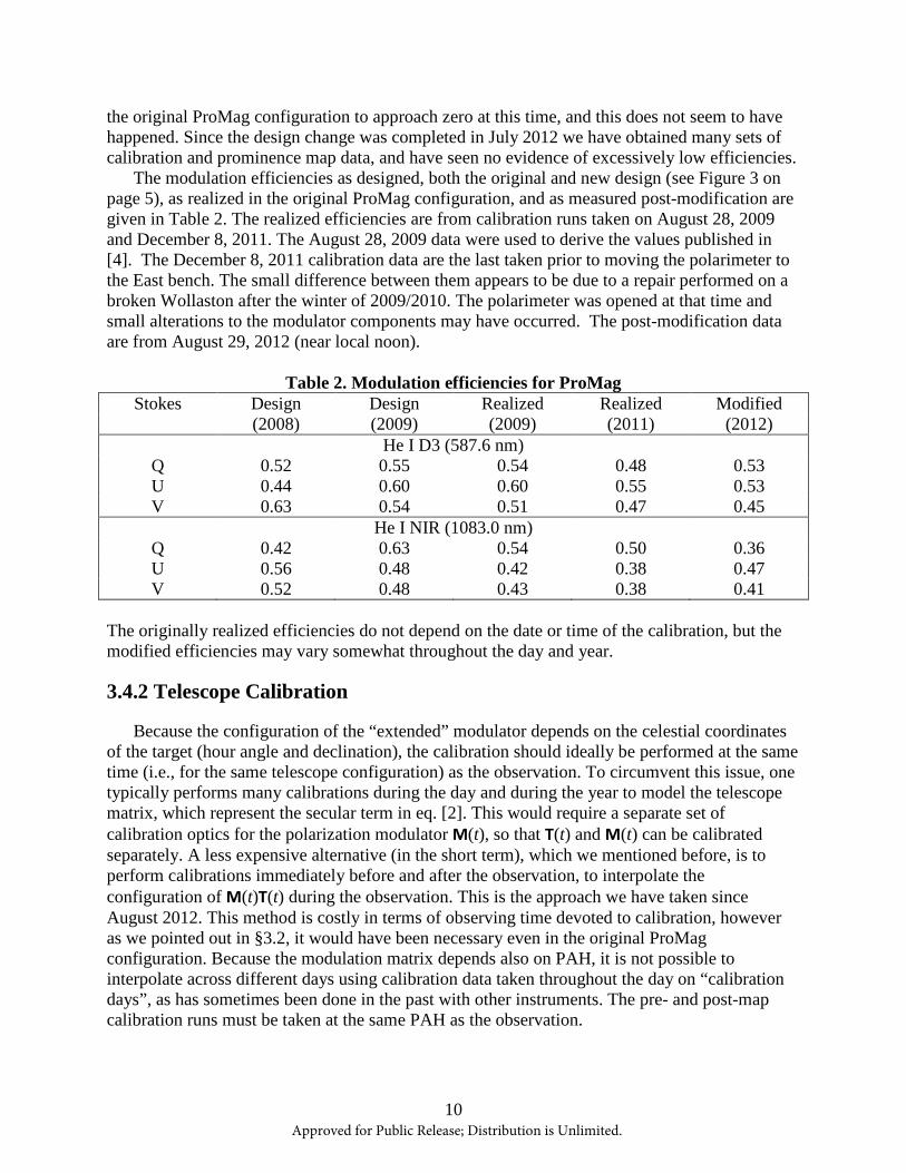
the original ProMag configuration to approach zero at this time, and this does not seem to have happened. Since the design change was completed in July 2012 we have obtained many sets of calibration and prominence map data, and have seen no evidence of excessively low efficiencies. The modulation efficiencies as designed, both the original and new design (see Figure 3 on page 5), as realized in the original ProMag configuration, and as measured post-modification are given in Table 2. The realized efficiencies are from calibration runs taken on August 28, 2009 and December 8, 2011. The August 28, 2009 data were used to derive the values published in [4]. The December 8, 2011 calibration data are the last taken prior to moving the polarimeter to the East bench. The small difference between them appears to be due to a repair performed on a broken Wollaston after the winter of 2009/2010. The polarimeter was opened at that time and small alterations to the modulator components may have occurred. The post-modification data are from August 29, 2012 (near local noon).

Table 2. Modulation efficiencies for ProMag Stokes Design Design Realized Realized Modified

(2008) (2009) (2009) (2011) (2012) He I D3 (587.6 nm)

Q 0.52 0.55 0.54 0.48 0.53 U 0.44 0.60 0.60 0.55 0.53 V 0.63 0.54 0.51 0.47 0.45

He I NIR (1083.0 nm) Q 0.42 0.63 0.54 0.50 0.36 U 0.56 0.48 0.42 0.38 0.47 V 0.52 0.48 0.43 0.38 0.41

The originally realized efficiencies do not depend on the date or time of the calibration, but the modified efficiencies may vary somewhat throughout the day and year.

3.4.2 Telescope Calibration

Because the configuration of the “extended” modulator depends on the celestial coordinates of the target (hour angle and declination), the calibration should ideally be performed at the same time (i.e., for the same telescope configuration) as the observation. To circumvent this issue, one typically performs many calibrations during the day and during the year to model the telescope matrix, which represent the secular term in eq. [2]. This would require a separate set of calibration optics for the polarization modulator M(t), so that T(t) and M(t) can be calibrated separately. A less expensive alternative (in the short term), which we mentioned before, is to perform calibrations immediately before and after the observation, to interpolate the configuration of M(t)T(t) during the observation. This is the approach we have taken since August 2012. This method is costly in terms of observing time devoted to calibration, however as we pointed out in §3.2, it would have been necessary even in the original ProMag configuration. Because the modulation matrix depends also on PAH, it is not possible to interpolate across different days using calibration data taken throughout the day on “calibration days”, as has sometimes been done in the past with other instruments. The pre- and post-map calibration runs must be taken at the same PAH as the observation.


3.4.3 Focus

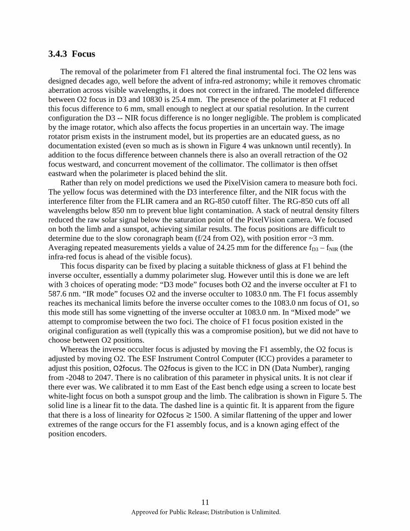
The removal of the polarimeter from F1 altered the final instrumental foci. The O2 lens was designed decades ago, well before the advent of infra-red astronomy; while it removes chromatic aberration across visible wavelengths, it does not correct in the infrared. The modeled difference between O2 focus in D3 and 10830 is 25.4 mm. The presence of the polarimeter at F1 reduced this focus difference to 6 mm, small enough to neglect at our spatial resolution. In the current configuration the D3 -- NIR focus difference is no longer negligible. The problem is complicated by the image rotator, which also affects the focus properties in an uncertain way. The image rotator prism exists in the instrument model, but its properties are an educated guess, as no documentation existed (even so much as is shown in Figure 4 was unknown until recently). In addition to the focus difference between channels there is also an overall retraction of the O2 focus westward, and concurrent movement of the collimator. The collimator is then offset eastward when the polarimeter is placed behind the slit. Rather than rely on model predictions we used the PixelVision camera to measure both foci. The yellow focus was determined with the D3 interference filter, and the NIR focus with the interference filter from the FLIR camera and an RG-850 cutoff filter. The RG-850 cuts off all wavelengths below 850 nm to prevent blue light contamination. A stack of neutral density filters reduced the raw solar signal below the saturation point of the PixelVision camera. We focused on both the limb and a sunspot, achieving similar results. The focus positions are difficult to determine due to the slow coronagraph beam (f/24 from O2), with position error ~3 mm. Averaging repeated measurements yields a value of 24.25 mm for the difference fD3 – fNIR (the infra-red focus is ahead of the visible focus). This focus disparity can be fixed by placing a suitable thickness of glass at F1 behind the inverse occulter, essentially a dummy polarimeter slug. However until this is done we are left with 3 choices of operating mode: “D3 mode” focuses both O2 and the inverse occulter at F1 to 587.6 nm. “IR mode” focuses O2 and the inverse occulter to 1083.0 nm. The F1 focus assembly reaches its mechanical limits before the inverse occulter comes to the 1083.0 nm focus of O1, so this mode still has some vignetting of the inverse occulter at 1083.0 nm. In “Mixed mode” we attempt to compromise between the two foci. The choice of F1 focus position existed in the original configuration as well (typically this was a compromise position), but we did not have to choose between O2 positions. Whereas the inverse occulter focus is adjusted by moving the F1 assembly, the O2 focus is adjusted by moving O2. The ESF Instrument Control Computer (ICC) provides a parameter to adjust this position, O2focus. The O2focus is given to the ICC in DN (Data Number), ranging from -2048 to 2047. There is no calibration of this parameter in physical units. It is not clear if there ever was. We calibrated it to mm East of the East bench edge using a screen to locate best white-light focus on both a sunspot group and the limb. The calibration is shown in Figure 5. The solid line is a linear fit to the data. The dashed line is a quintic fit. It is apparent from the figure that there is a loss of linearity for O2focus ≳ 1500. A similar flattening of the upper and lower extremes of the range occurs for the F1 assembly focus, and is a known aging effect of the position encoders.


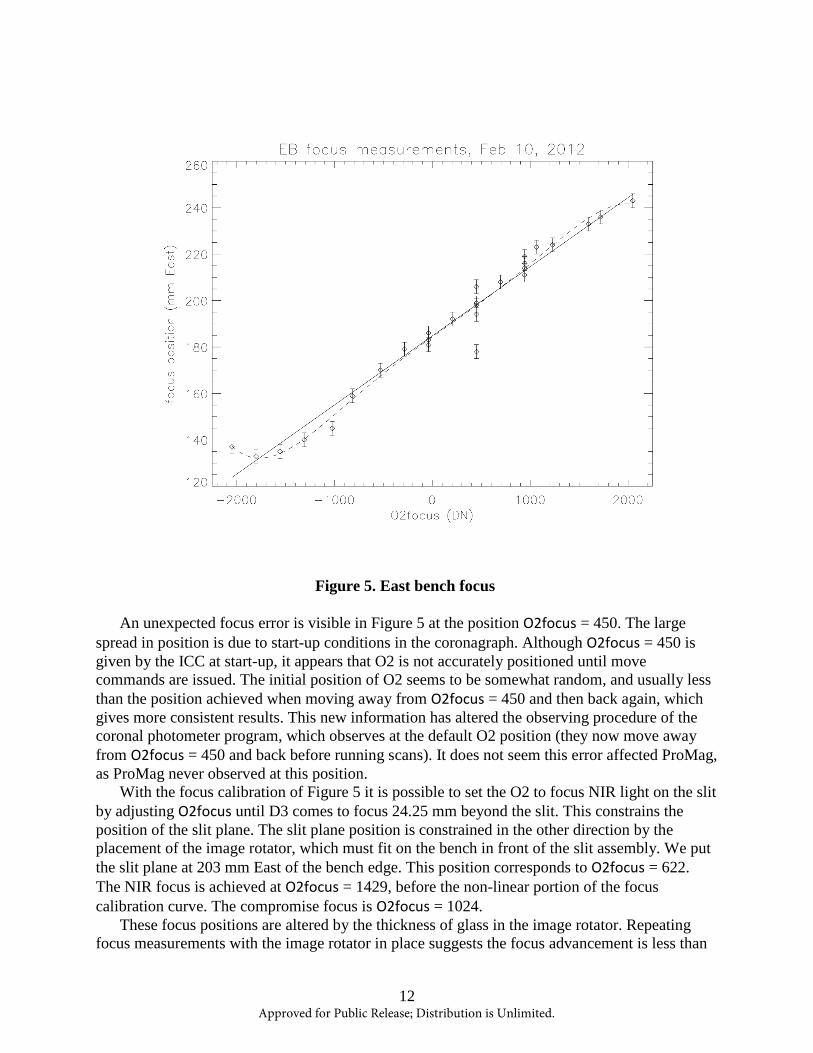
Figure 5. East bench focus

An unexpected focus error is visible in Figure 5 at the position O2focus = 450. The large spread in position is due to start-up conditions in the coronagraph. Although O2focus = 450 is given by the ICC at start-up, it appears that O2 is not accurately positioned until move commands are issued. The initial position of O2 seems to be somewhat random, and usually less than the position achieved when moving away from O2focus = 450 and then back again, which gives more consistent results. This new information has altered the observing procedure of the coronal photometer program, which observes at the default O2 position (they now move away from O2focus = 450 and back before running scans). It does not seem this error affected ProMag, as ProMag never observed at this position. With the focus calibration of Figure 5 it is possible to set the O2 to focus NIR light on the slit by adjusting O2focus until D3 comes to focus 24.25 mm beyond the slit. This constrains the position of the slit plane. The slit plane position is constrained in the other direction by the placement of the image rotator, which must fit on the bench in front of the slit assembly. We put the slit plane at 203 mm East of the bench edge. This position corresponds to O2focus = 622. The NIR focus is achieved at O2focus = 1429, before the non-linear portion of the focus calibration curve. The compromise focus is O2focus = 1024. These focus positions are altered by the thickness of glass in the image rotator. Repeating focus measurements with the image rotator in place suggests the focus advancement is less than


3 mm, essentially below the measurement error. It appears that the image rotator prisms were carefully designed, so that the focus displacement due to the prism glass is neatly removed by the sideways displacement of light from the beam path. An index of refraction n=1.5 for the prism glass would account for this. The image rotator focus displacement in the infra-red is unknown. Refractive index values for common optical glasses, with n ≈ 1.5 in the visible, suggest a further displacement of the IR (infrared; 1083.0 nm) focus by ≈ 1 mm, a negligible amount given the f-ratio of the beam.

3.5 Calibration

While the spectrographic information can be analyzed immediately, to meet the ultimate goal of measuring full vector prominence magnetic field requires a careful polarimetric calibration, with high precision (~10-3). Calibration data are taken using the calibration optics located at F1. These two optical devices rotate independently from one another during the calibration process. This creates (theoretically) known input Stokes vectors from which calibration parameters can be found. Each calibration set consists of 48 images. The first 4 are clear images without the polarizer or retarder in the beam; these are followed by 2 dark images. 36 calibration images, divided into three groups of twelve, are then taken. These three groups are distinguished by the angle of the retarder, which rotates 60° every twelve images. The polarizer rotates 15° with each image. This consistent rotation creates a smooth periodic variation in intensity between the two beams, with a discontinuity every twelve images when the retarder rotates. This intensity variation is shown in Figure 6 for the two orthogonally-linear-polarized beams. Arrows point to the last frame in a set of 12, after which the calibration retarder rotates 60°. The 36 calibration images are then followed by another set of 2 dark images and 4 clear images. The entire process takes ≈13:50 minutes. In that time the telescope moves ≈4˚ in RA, and the image rotator moves 2˚. Declination movement is small over the course of one day (with the possible exception of days close to the equinoxes).

Figure 6. Total intensity of calibration images


These calibration data must be inverted to modulation matrix parameters in order to produce Stokes maps from the 4 camera signals. Strictly speaking the modulation matrix resulting from these calibrations must be an average over the modulation variance during the ~14 minutes required to obtain the data. Our present approach uses a calibration model with 25 parameters. 16 parameters are the components of the 4x4 modulation matrix of the telescope plus modulator combination. These can be reduced to 12 parameters by forcing the first column of the modulation matrix to 1.0. The remaining 9 parameters are the input Stokes vector (4), the CCD bias (1), the calibration optics transmittance and retardance (2), and offset angles for the calibration retarder and polarizer (2 -- these account for any residual error in the calibration optics reference directions). The calibration analysis program minimizes the χ2 fit to the data using a Monte-Carlo approach. Two different minimization algorithms are used, Latin Hypercube Sampling (LHS), and Amoeba (Downhill Simplex). The Amoeba is a fairly robust deterministic minimizer which does not require derivative information to find its way downhill. We have incorporated a Monte-Carlo approach with the Amoeba by initializing it using a random perturbation around an initial guess (which might be from a previous run using LHS or from the polarimeter design) to more fully sample the parameter space. Latin Hypercube Sampling is an inherently Monte-Carlo process which widely samples the parameter space, with subsequent iterations restricting the parameter space to smaller regions around the minimum. For further discussion of these two algorithms see [5].

3.6 Observation Sequence

We select target prominences using H-alpha images from the Global Oscillation Network Group (GONG), of which Figure 7 is an example. We also use other data sets for further context and guidance in selecting targets, including NASA Solar Dynamics Observatory Atmospheric Imaging Assembly (SDO/AIA) 304 channel (which shows primarily He II emission), ISOON He I 10830 images (when available), and the AFRL coronal photometer Ca XV channel . Ca XV coronal photometer scans are taken every day in the morning, and when Ca XV activity is

Figure 7. Gong image from June 18, 2013. The circled prominence is the target14


observed and a prominence is seen at the same location we always select it. GONG images are loaded into PMGONG, an IDL program, which assists in determining the heliocentric position angle of the selected prominence. Rotation angles of the inverse occulter at F1 and image rotator are both determined from heliocentric position angle by the program PROMAGSET. Every spectro-polarimetric map is bracketed by calibration sets taken at the same heliocentric position angle as the prominence. The pre-map and post-map calibrations are limb calibrations -- performed near the limb so as to more precisely match the telescope position used for the map (for prominence maps; calibrations are performed at the same location as the filament for filament maps). In addition to these, every observation day begins and ends with a calibration set at the geocentric position angle of 0°. Some observing days are given over mostly or entirely to calibrations taken in a “running” mode, in which calibrations follow each other immediately. These calibration data allow us to track the daily and yearly time variation of the modulation matrix, as they are all taken at the same PAH. Normally this is actually PAG=0 (geocentric position angle).

4. RESULTS AND DISCUSSION

Since the removal of the polarimeter to the East bench we have obtained data at a steady pace. Calibrations are performed before and after each prominence map, as well as at intervals throughout the day, so calibration data predominate. Prominence observations are run daily (weather permitting). We have data in the new instrument mode (polarimeter at East bench) from August, 2012 to the present. From August 2012 – July 2014 (inclusive) we had 172 observing days, yielding 535 maps of 284 prominences of all types and sizes, including some which were observed immediately before, during, or after an eruption event (or even all three for the same event). Based on contemporaneous observing notes there appear to be 10 eruptive prominences observed in our data-set (it is not always clear whether a prominence is erupting until afterward). One was observed 5 times during the complete evolution of its eruption, both before (one map), during (three maps), and after (one map) the eruption, which left behind a remnant. Our long-term calibration run to prominence map ratio is nearly 3:1. Because calibration runs are always faster than maps the calibration to prominence ratio is close to 1:1 in terms of observing time. Figure 8 shows the extent of data coverage since the changes were completed in July 2012. Symbols indicate the type of data taken, + for calibrations, ◊ for science targets. Both science maps (prominences and filaments) and the associated calibrations are shown, as well as periods of running mode calibration (visible as a series of + symbols spaced regularly in time).


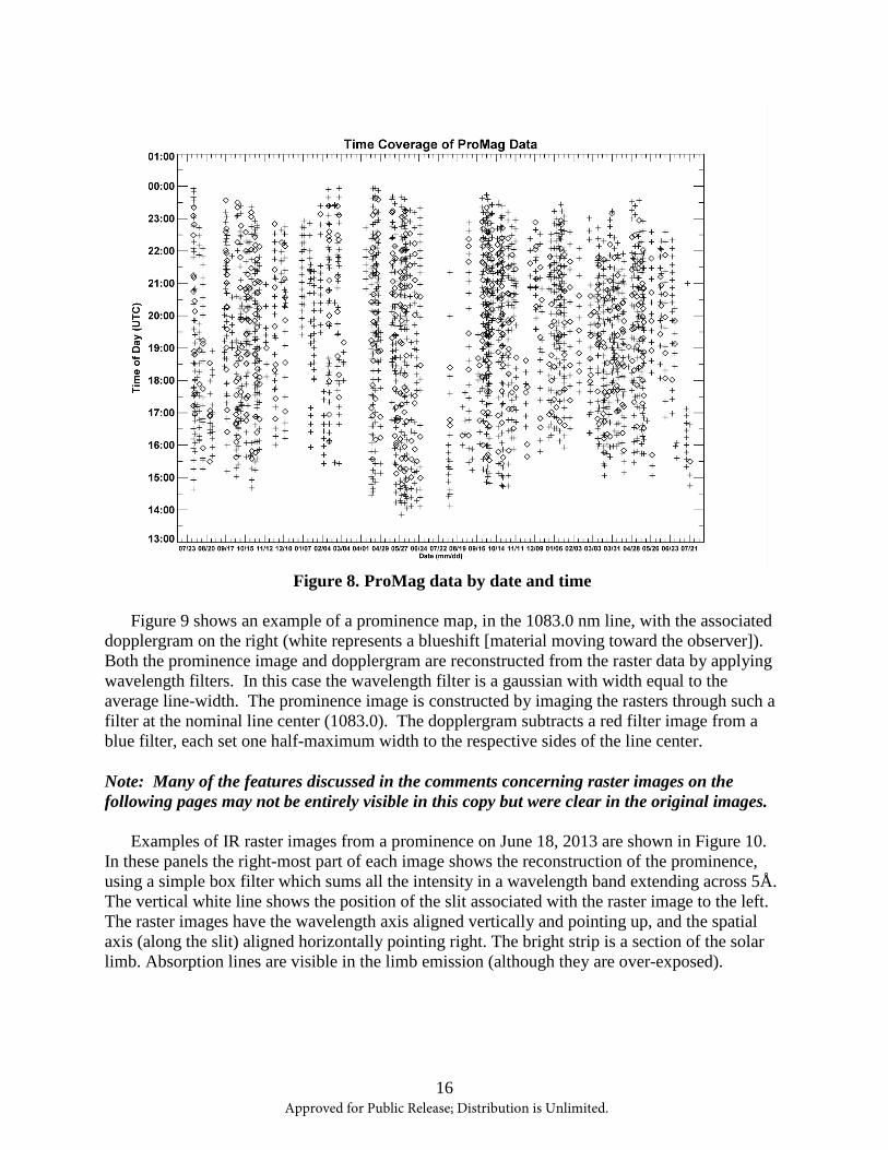
Figure 8. ProMag data by date and time

Figure 9 shows an example of a prominence map, in the 1083.0 nm line, with the associated dopplergram on the right (white represents a blueshift [material moving toward the observer]). Both the prominence image and dopplergram are reconstructed from the raster data by applying wavelength filters. In this case the wavelength filter is a gaussian with width equal to the average line-width. The prominence image is constructed by imaging the rasters through such a filter at the nominal line center (1083.0). The dopplergram subtracts a red filter image from a blue filter, each set one half-maximum width to the respective sides of the line center.

Note: Many of the features discussed in the comments concerning raster images on the following pages may not be entirely visible in this copy but were clear in the original images.

Examples of IR raster images from a prominence on June 18, 2013 are shown in Figure 10. In these panels the right-most part of each image shows the reconstruction of the prominence, using a simple box filter which sums all the intensity in a wavelength band extending across 5Å. The vertical white line shows the position of the slit associated with the raster image to the left. The raster images have the wavelength axis aligned vertically and pointing up, and the spatial axis (along the slit) aligned horizontally pointing right. The bright strip is a section of the solar limb. Absorption lines are visible in the limb emission (although they are over-exposed).


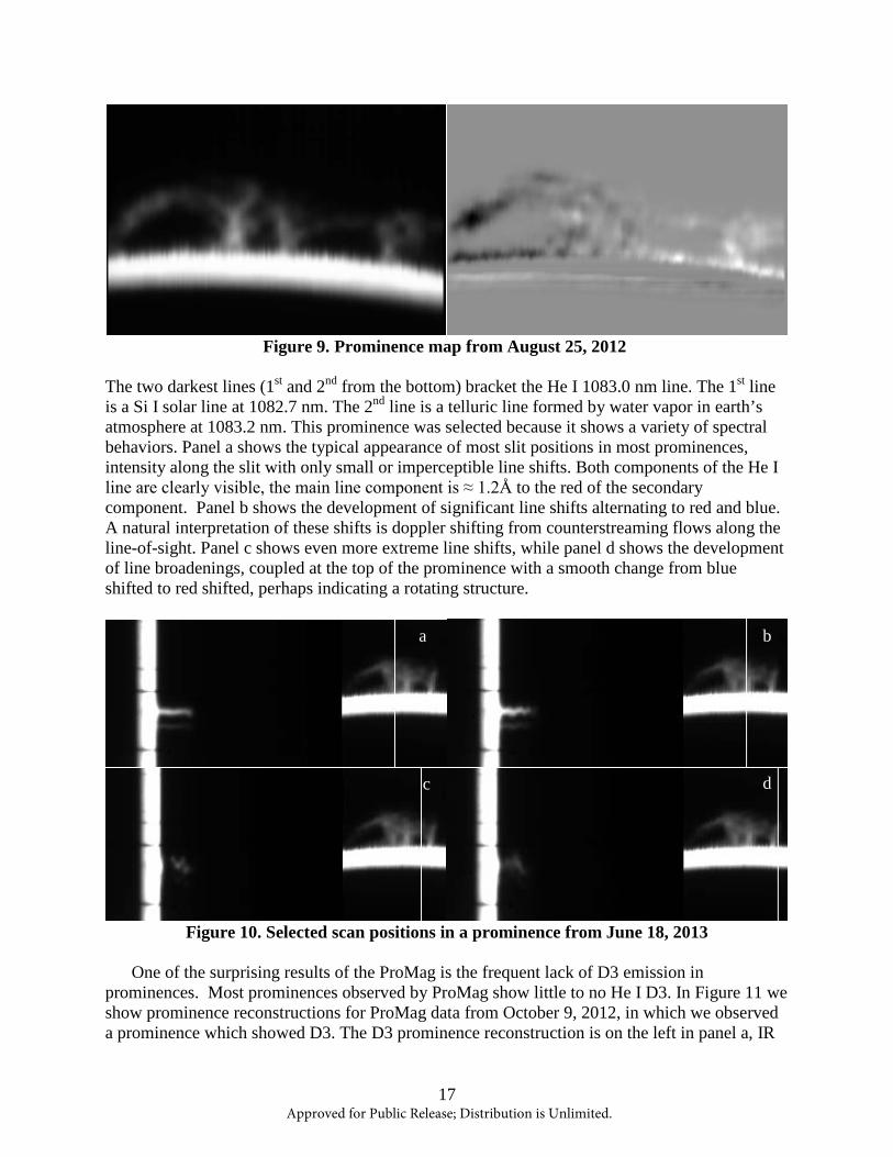
Figure 9. Prominence map from August 25, 2012

The two darkest lines (1st and 2nd from the bottom) bracket the He I 1083.0 nm line. The 1st line is a Si I solar line at 1082.7 nm. The 2nd line is a telluric line formed by water vapor in earth’s atmosphere at 1083.2 nm. This prominence was selected because it shows a variety of spectral behaviors. Panel a shows the typical appearance of most slit positions in most prominences, intensity along the slit with only small or imperceptible line shifts. Both components of the He I line are clearly visible, the main line component is ≈ 1.2Å to the red of the secondary component. Panel b shows the development of significant line shifts alternating to red and blue. A natural interpretation of these shifts is doppler shifting from counterstreaming flows along the line-of-sight. Panel c shows even more extreme line shifts, while panel d shows the development of line broadenings, coupled at the top of the prominence with a smooth change from blue shifted to red shifted, perhaps indicating a rotating structure.

Figure 10. Selected scan positions in a prominence from June 18, 2013

One of the surprising results of the ProMag is the frequent lack of D3 emission in prominences. Most prominences observed by ProMag show little to no He I D3. In Figure 11 we show prominence reconstructions for ProMag data from October 9, 2012, in which we observed a prominence which showed D3. The D3 prominence reconstruction is on the left in panel a, IR

a b

c d


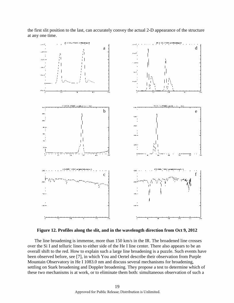
on the right (panel b). Both polarization beams have been shown here, as observed, one above the other. The D3 limb appears much thicker because the data were taken in IR mode, when the telescope was set up with both the occulter and O2 focused to the 1083.0 nm settings. This particular prominence was also observed by many other instruments, including the Dunn Solar Telescope, and THÉMIS. These data show He I D3 emission which is very strong compared to a typical ProMag observation. Figure 12 shows dark-subtracted, but otherwise raw data slices taken through the brightest region of the prominence, both along the slit (panels a, d), and along the wavelength axis (panels b, e), as well as a wavelength slice taken from the limb emission (panels c, f), showing the absorption spectrum in the vicinity of the He I lines. Panels a-c are from the D3 data, panels d-f are from the IR. The relative intensity of D3 and IR emission can be seen by the prominence to limb ratio in panels a and d, and the more noisy appearance of the wavelength profile in Figure 12b. However, the D3 line is well sampled in these data, and the secondary component is resolved.

Figure 11. Prominence reconstructions from October 9, 2012 in both D3 (a) and IR (b)

In addition to prominences, ProMag has also observed post-flare loops associated with flares near the limb. At first this was an accident, as it can be difficult to tell the difference between loops rising above the limb, and prominences from a single GONG H-α image. However, upon seeing the unusual spectral profile of these events we began to observe post-flare loops as targets of opportunity. We now have many examples in our dataset. The post-flare loop data shown in Figure 13 and Figure 14 is from the first event that we recognized as such on May 22, 2013 (in retrospect we found that we had previously observed others as well, without realizing it at the time). It should be noted that the IR “prominence” reconstruction in Figure 13 gives a misleading impression of the appearance of the loops. No 2-D snapshot of the loops would look exactly like the reconstruction shown. The post-flare loops are highly dynamic, changing significantly during the mapping time. No reconstruction from our slit spectra of an object which has changed from

a b


the first slit position to the last, can accurately convey the actual 2-D appearance of the structure at any one time.

Figure 12. Profiles along the slit, and in the wavelength direction from Oct 9, 2012

The line broadening is immense, more than 150 km/s in the IR. The broadened line crosses over the Si I and telluric lines to either side of the He I line center. There also appears to be an overall shift to the red. How to explain such a large line broadening is a puzzle. Such events have been observed before, see [7], in which You and Oertel describe their observation from Purple Mountain Observatory in He I 1083.0 nm and discuss several mechanisms for broadening, settling on Stark broadening and Doppler broadening. They propose a test to determine which of these two mechanisms is at work, or to eliminate them both: simultaneous observation of such a

a

b

c

d

e

f


broadened line in both He I D3 and 1083.0. The ratio of widths in the two He I lines is a diagnostic of the broadening mechanism, and differs dramatically for Stark broadening and Doppler broadening. This is a test which we can perform with ProMag, providing there is enough D3 emission observed to permit a measurement of the line width. A sample D3 line profile from the May 22, 2013 event is shown in Figure 14a. The D3 emission in this case was very faint, but detectable. It remains to be seen whether a consistent measure of line width can be determined from these data.

Figure 13. Post-flare loop observation from May 22, 2013

Figure 14. Line profiles from the May 22, 2013 post-flare loop

Observations of eruptive, as well as non-eruptive, prominences are necessary to further the ultimate goal of the ProMag program: prediction of prominence eruptions. However, because we currently have no way to predict eruptions, our ability to observe them depends on luck. We must simply observe as many prominences as we can and hope that some of them will happen to erupt during or shortly after our observation.

The number of eruptive or pre-eruptive prominences observed with ProMag is about 10. More than half of that number were observed recently (since Jan. 2014) as a natural consequence of the progress of the solar cycle into its declining phase. The best observation of an eruptive prominence to date occurred on April 29, 2014. That event was mapped 5 times in succession, just before, during (3x), and just after the eruption. Figure 15 to Figure 20 document its main spectral features in the IR.

a b


Figure 15 shows the succession of map reconstruction images for the 5 maps. As with post-flare loops, no single moment during the eruption would have looked like the reconstructions shown, as the prominence is undergoing rapid change while we are scanning it. The post-eruption map is of a small remnant left behind by the main eruption. The remnant portion persists throughout the eruption with relatively ordinary spectral profiles. Other slit positions show more interesting spectral behaviors. Figure 16 through Figure 20 show some representative examples map by map. Each of Figure 16 through Figure 20 corresponds with one of the reconstructions in Figure 15. The map reconstruction is displayed with each spectral raster position indicated by the white line, as before (see Figure 10).

Figure 16 shows a single raster from the pre-eruption map. Most of the other rasters are

ordinary (like Figure 10a) or are like this one, some line shifts going up along the slit, with a sudden enormous redshift at the top of the prominence. The shear is extreme, more than 100 km/s in velocity units. Figure 17 shows four rasters from the start of the eruption. Some are not

much changed from the pre-eruption state, such as Figure 17a, or Figure 17b which shows the remnant portion, now overlain by a spreading arm of the highly red-shifted component (which may not be visible in this copy). Panel c appears to show the development of a continuous trend from blueshift to redshift. Panel d shows separation into discontinuous layers with dramatically

Figure 15. Succession of map reconstructions for the April 29, 2014 eruptive prominence

Figure 16. Raster from the pre-eruption map, beginning 183621 UTC

Figure 17. Rasters from the 1st eruption map, beginning 193505 UTC

a b

c d


different line shifts. Figure 18 and 19 show bizarre spectral behaviors, with both line shifts (mostly to the red) and broadenings which are extreme (more than 5 - 6Å away from the normal line center). Without more careful analysis, including polarimetric calibration, we can only guess at the causes of these unusual spectral signatures. Other eruptive prominences we have observed also show spectra similar in character to the 7 panels in figure 18 and figure 19.

The post-eruption remnant in Figure 20 is back to mostly typical spectral behavior, with line centers near the nominal value, and an ordinary line broadening at the top of the prominence.

Such a sudden broadening, growing quickly out of a typical prominence spectrum, is by no means typical prominence behavior, however. Even by this time in the course of the eruption faint wisps of material remain that show the more unusual spectral signatures of figure 18 and figure 19.

Figure 18. Rasters from the 2nd eruption map, beginning 203824 UTC

a b

c d

Figure 19. Rasters from the 3rd eruption map, beginning 212534 UTC

a b

c


4.1 Calibration Results

In order to invert ProMag data to Stokes maps and from there produce maps of vector magnetic field and other physical quantities we must have robust calibration results. Although much progress in this direction has been made, lingering problems have prevented us from performing the magnetic field measurement as yet. In this section we will show some of the results of present calibration analysis and discuss the issues which still need to be resolved.

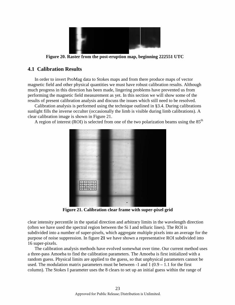
Calibration analysis is performed using the technique outlined in §3.4. During calibrations sunlight fills the inverse occulter (occasionally the limb is visible during limb calibrations). A clear calibration image is shown in Figure 21.

A region of interest (ROI) is selected from one of the two polarization beams using the 85th

clear intensity percentile in the spatial direction and arbitrary limits in the wavelength direction (often we have used the spectral region between the Si I and telluric lines). The ROI is subdivided into a number of super-pixels, which aggregate multiple pixels into an average for the purpose of noise suppression. In figure 21 we have shown a representative ROI subdivided into 16 super-pixels.

The calibration analysis methods have evolved somewhat over time. Our current method uses a three-pass Amoeba to find the calibration parameters. The Amoeba is first initialized with a random guess. Physical limits are applied to the guess, so that unphysical parameters cannot be used. The modulation matrix parameters must be between -1 and 1 (0.9 – 1.1 for the first column). The Stokes I parameter uses the 8 clears to set up an initial guess within the range of

Figure 20. Raster from the post-eruption map, beginning 222551 UTC

Figure 21. Calibration clear frame with super-pixel grid


measured intensities, and Stokes QUV are normalized by I and forced to lie between -0.5 and 0.5. The transmission of the calibration optics must be between 0 and 1, and the retardance between 0˚ and 180˚. The calibration angle offsets are initialized to within ±1˚ of the nominal values measured independently when the instrument was first deployed, 0.5˚ for the polarizer and 3.9˚ for the retarder. Any angle would be permissible physically, but we trust the original measurement to within 1˚. At one time the bias parameter was initialized using the darks, but we found that it works much better to simply subtract the darks from the data and dispense with the bias parameter. We have also fixed the 1st modulation matrix element to a constant value of 1 (this amounts to a choice of an overall scaling factor of the modulation matrix), so in practice we do not use the more general 25 parameter model anymore. The Amoeba routine is then used to find the minimum χ2 starting from this random initial guess. Each super-pixel is run independently, achieving an independent solution. The results of all super-pixels are averaged with χ2 weighting. This average solution is used with a random offset for each super-pixel (applying the same physical limits; in fact the Amoeba routine is also constrained with the same limits so that it does not attempt any solution which would be unphysical) to initialize the 2nd pass of Amoeba. The χ2 weighted average solution from this 2nd pass initializes the 3rd pass, with a random offset to each parameter 1/5 as large. The output of the last pass is taken as the solution.

4.2 Time variability of the Extended Modulator

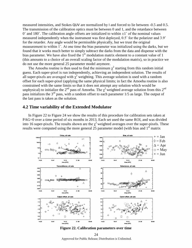
In Figure 22 to Figure 24 we show the results of this procedure for calibration sets taken at PAG=0 over a time period of six months in 2013. Each set used the same ROI, and was divided into 16 super-pixels. The results shown are the χ2 weighted averages over the super-pixels. These results were computed using the more general 25 parameter model (with bias and 1st matrix

Figure 22. Calibration parameters over time

+ = Jan ◊ = Feb∆ = Apr □ = May× = Jun


element). Figure 22 shows the final average χ2, the bias, calibration transmittance, retardance, and offset angles (for these inversions we used base values of 0˚). The horizontal axis is time of day in UTC, and the plot symbols designate the month of the year according to the legend. March 2013 is missing because no calibration data were taken in that month. This is unfortunate since that is the time nearest to the equinox when we would expect the calibration parameters to be changing most rapidly with respect to day-of-year (the solar declination changes quickly around the equinoxes).

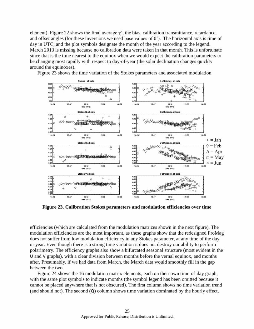
Figure 23 shows the time variation of the Stokes parameters and associated modulation

efficiencies (which are calculated from the modulation matrices shown in the next figure). The modulation efficiencies are the most important, as these graphs show that the redesigned ProMag does not suffer from low modulation efficiency in any Stokes parameter, at any time of the day or year. Even though there is a strong time variation it does not destroy our ability to perform polarimetry. The efficiency graphs also show a bifurcated seasonal structure (most evident in the U and V graphs), with a clear division between months before the vernal equinox, and months after. Presumably, if we had data from March, the March data would smoothly fill in the gap between the two. Figure 24 shows the 16 modulation matrix elements, each on their own time-of-day graph, with the same plot symbols to indicate months (the symbol legend has been omitted because it cannot be placed anywhere that is not obscured). The first column shows no time variation trend (and should not). The second (Q) column shows time variation dominated by the hourly effect,

Figure 23. Calibration Stokes parameters and modulation efficiencies over time

+ = Jan ◊ = Feb∆ = Apr □ = May× = Jun


which repeats nearly the same pattern each day. The seasonal variation has only a small effect on Q. The Q-to-Q element (2nd row, 2nd column) does not seem to show a clear trend with time. We do not know what to make of this. The UV columns show the bifurcated seasonal trends, with strong daily variation superposed on a weaker seasonal variation. The more visible seasonal

trend in these two columns leads directly to the visibility of the seasonal trend in the associated efficiencies. In some of the UV matrix elements the April data (denoted with an up-pointing triangle, ∆) appears in both curves, or even between them. This is because the April calibration data come from two days, one at the beginning of the month (about 2 weeks after equinox) and one at the end. Although some fine-tuning of the procedure could perhaps clean up these graphs a little, the performance of the calibration code is quite good. The regular and physically reasonable appearance of the efficiency and modulation curves, give us confidence in the calibration method. It is also significant that no very low efficiencies are found at any time. This demonstrates the alterations we made to the instrument are tenable.

4.3 Stability Analysis

The first thing we discovered performing calibration inversions was a variation in calibration parameters with super-pixel. Since this was unexpected we performed a stability analysis of the code to determine if the variations were artifacts of the random initialization. We do this by re-

Figure 24. Calibration modulation matrix over time


running the full 3 pass algorithm a large number of times with the same input data. The repeated random initializations allow us to explore a large portion of the parameter space. Figures 25 - 30 show an example of the output of one such run. This run is for NIR calibration data from April 16, 2013 and is performed on the 1st beam. These 150 runs for each of 50 super-pixels were performed with the 3-pass Amoeba minimization. The super-pixels are 1×32 pixels, averaging over wavelength, but fully resolved along the slit (we find the largest variations along the slit). The lines show the position of the median of the 150 values for each super-pixel. The Median Absolute Deviation from the Median (MADM) is displayed by the error bar (extending from median-MADM to median+MADM, containing the middle 50% of points). In some figures the error bars are so small they are not readily discernible. Medians and MADM are used because these measures of central tendency and width are strongly robust against outliers, which are often present. These statistics require no potentially sensitive choices on the part of the experimenter, as e.g. a truncated mean (which requires the choice of percentage of high and low points discarded). We have found and fixed many code bugs, the code now is very stable; most runs end up in almost the same place, scatter is low, and outliers are rarer (although still present). Also we are now using large numbers of super-pixels (to fully resolve the spatial variation along the slit).

Figure 25. χ2 for a calibration set taken April 16, 2013 at 194201 UTC

Figure 25 shows the χ2 from this set. The error bars are so small they look like lines. The statistical variation is several orders of magnitude smaller than the χ2. These values of χ2 are quite good. We have 14 degrees of freedom in our model (23 parameters and 37 data points per super-pixel), so the best value of χ2 is 14.

Figure 26 shows the calibration optics combined retardance and transmittance. The calibration optics cannot be inserted in the beam separately so only combined values can be extracted. The trends could be artifacts (in particular the calibration model is relatively insensitive to small variations in retardance), but it is not a statistical artifact. The code consistently finds those values, so the trend is really in the data.


Figure 26. Calibration retardance and transmittance

Figure 27 shows the calibration optics offsets. The values stay near the nominal values and the scatter here is large. It is possible that one or both of these offsets are unmeasurable using this calibration procedure. Runs performed with either of the offsets initialized differently (e.g. from 0) result in widely different values than are found here, while still producing low values of χ2.However, the difference between the offsets is robust. There are physical reasons for expecting

Figure 27. Calibration polarizer and retarder offset angles that only the difference can be detected (the choice of polarizer offset essentially sets the origin of the coordinate system). Figure 28 displays all four Stokes components with their associated modulation efficiency. Once again, the statistical variation is almost imperceptible. The fall-off in efficiency at the lower portion of the slit is real (at least it is not a statistical artifact), and does not always occur. It seems to be worse the more the image falls towards the bottom of the slit plane (the occulted image of the corona wanders on the focal plane due to telescope and image rotator mis-alignments).


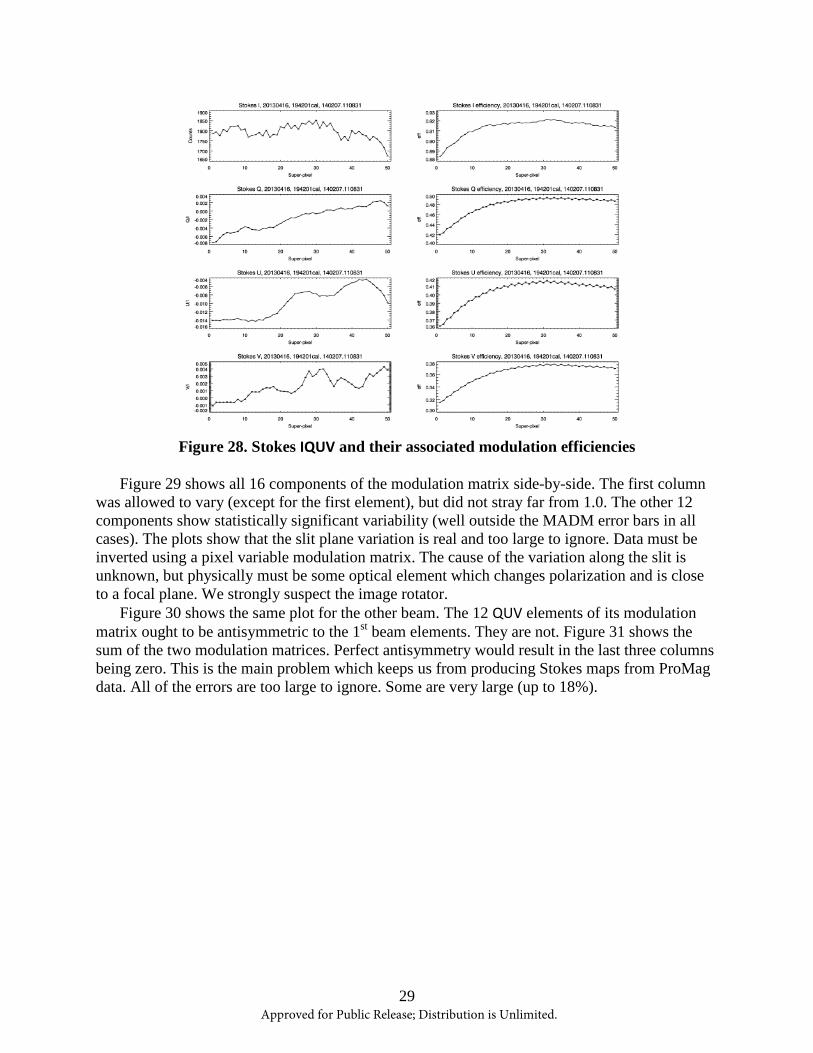
Figure 28. Stokes IQUV and their associated modulation efficiencies

Figure 29 shows all 16 components of the modulation matrix side-by-side. The first column was allowed to vary (except for the first element), but did not stray far from 1.0. The other 12 components show statistically significant variability (well outside the MADM error bars in all cases). The plots show that the slit plane variation is real and too large to ignore. Data must be inverted using a pixel variable modulation matrix. The cause of the variation along the slit is unknown, but physically must be some optical element which changes polarization and is close to a focal plane. We strongly suspect the image rotator. Figure 30 shows the same plot for the other beam. The 12 QUV elements of its modulation matrix ought to be antisymmetric to the 1st beam elements. They are not. Figure 31 shows the sum of the two modulation matrices. Perfect antisymmetry would result in the last three columns being zero. This is the main problem which keeps us from producing Stokes maps from ProMag data. All of the errors are too large to ignore. Some are very large (up to 18%).


Figure 29. Modulation matrix for April 16, 2013, 194201 UTC


Figure 30. Modulation matrix for the 2nd Beam


Figure 31. Sum of the modulation matrices from the two beams

4.4 Flat Fielding

The calibration data have not been flat-fielded. The introduction of a detector flat to our procedure is a necessary step, which we have not yet taken due to the difficulty in creating a robust flat-field procedure for this instrument. It is possible that the use of a correct flat field would help resolve the problem with the dual beam modulation matrices. Flat-fielding poses difficulty for our spectrographic instrument. We have no flat source, and any solar derived light (the most natural choice) contains the spectrum of sunlight in our two bands. We have made several attempts to produce a flat-field using a variation of the Kuhn method [6]. So far these attempts have not resulted in robust flat-fields. Figure 32 shows our best flat field in the IR to date using the Kuhn method. The right most portion of the flat field is not well sampled by our data (the two beams do not often illuminate that portion). This flat captures many of the defects of the detector, but is not adequate. Figure 33 shows an unflat clear on the left and a flat clear on the right using this flat field. The interference fringes are not removed, and may be worse. We have also attempted a post-analysis flattening of the data using Principal Component Analysis (PCA). Our PCA operates in the wavelength direction; we haven’t yet performed a 2-D


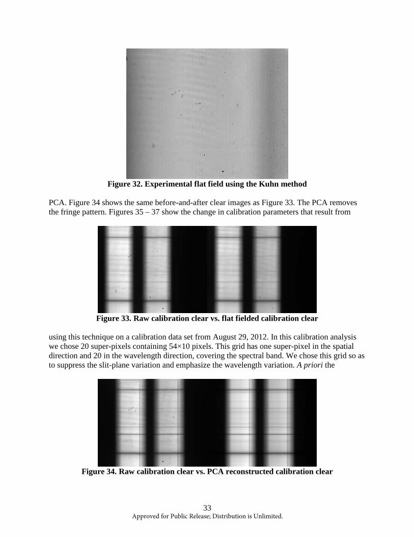
Figure 32. Experimental flat field using the Kuhn method

PCA. Figure 34 shows the same before-and-after clear images as Figure 33. The PCA removes the fringe pattern. Figures 35 – 37 show the change in calibration parameters that result from

Figure 33. Raw calibration clear vs. flat fielded calibration clear

using this technique on a calibration data set from August 29, 2012. In this calibration analysis we chose 20 super-pixels containing 54×10 pixels. This grid has one super-pixel in the spatial direction and 20 in the wavelength direction, covering the spectral band. We chose this grid so as to suppress the slit-plane variation and emphasize the wavelength variation. A priori the

Figure 34. Raw calibration clear vs. PCA reconstructed calibration clear


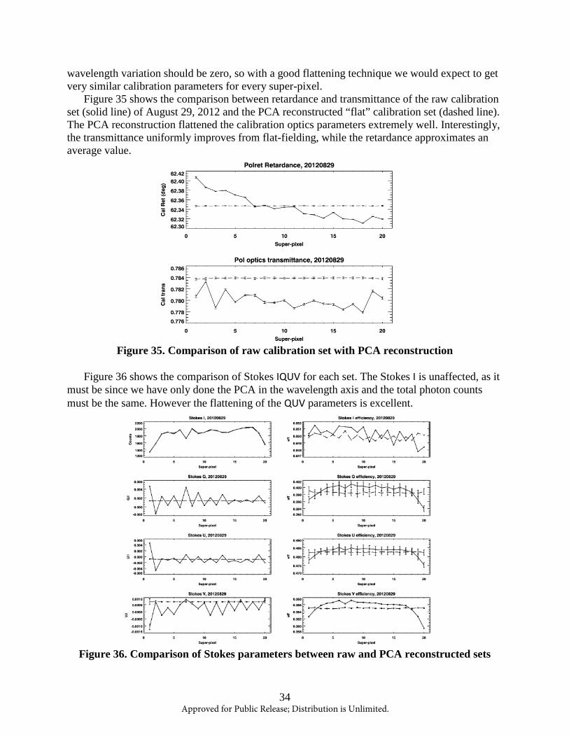
wavelength variation should be zero, so with a good flattening technique we would expect to get very similar calibration parameters for every super-pixel. Figure 35 shows the comparison between retardance and transmittance of the raw calibration set (solid line) of August 29, 2012 and the PCA reconstructed “flat” calibration set (dashed line). The PCA reconstruction flattened the calibration optics parameters extremely well. Interestingly, the transmittance uniformly improves from flat-fielding, while the retardance approximates an average value.

Figure 35. Comparison of raw calibration set with PCA reconstruction

Figure 36 shows the comparison of Stokes IQUV for each set. The Stokes I is unaffected, as it must be since we have only done the PCA in the wavelength axis and the total photon counts must be the same. However the flattening of the QUV parameters is excellent.

Figure 36. Comparison of Stokes parameters between raw and PCA reconstructed sets


Figure 36 also shows the modulation efficiency comparison. The Stokes V signal in particular is much improved, but the Q and U also get better. Figure 37 shows the modulation matrix for the raw calibration set and the PCA reconstructed set (solid and dashed lines as before). The improvement in the V elements is quite clear. Some of the Q and U elements do not seem to get a lot better, but they were relatively flat to begin with. The matrix elements which had large variations across wavelength have all been flattened quite well.

The PCA technique clearly does an excellent job of removing the wavelength axis variation. We have not yet tried to flatten in the slit direction using this technique. But how well does it resolve the antisymmetry issue between beams? Unfortunately it does not. The sum of beam modulation matrices still does not show 0 elements in the QUV columns. The variation in the sum is removed, and what remains is similar to the average of the previous variation. In other words, the discrepancy between beams is flattened out, but not removed. It would appear that the antisymmetry issue is not related to flat-fielding.

Figure 37. Modulation matrix for the raw and PCA reconstruction

5. CONCLUSIONS

Relative to [8], we changed the ProMag configuration in response to a difficulty in aligning the


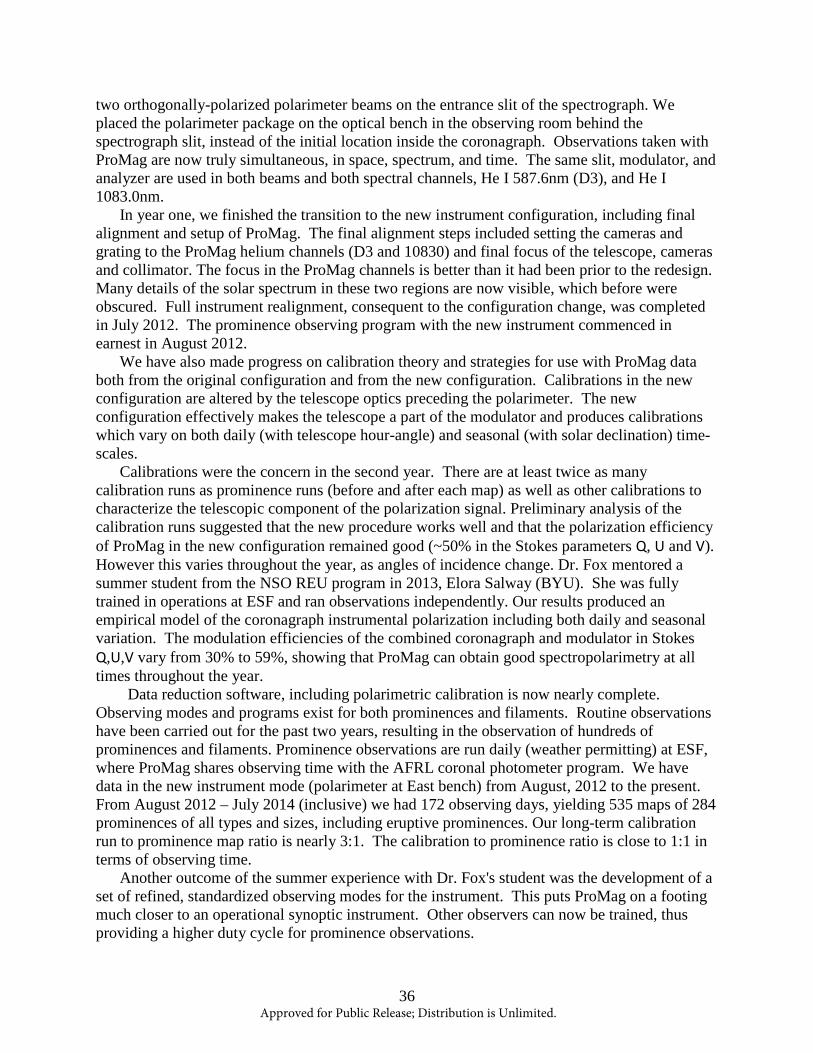
two orthogonally-polarized polarimeter beams on the entrance slit of the spectrograph. We placed the polarimeter package on the optical bench in the observing room behind the spectrograph slit, instead of the initial location inside the coronagraph. Observations taken with ProMag are now truly simultaneous, in space, spectrum, and time. The same slit, modulator, and analyzer are used in both beams and both spectral channels, He I 587.6nm (D3), and He I 1083.0nm.

In year one, we finished the transition to the new instrument configuration, including final alignment and setup of ProMag. The final alignment steps included setting the cameras and grating to the ProMag helium channels (D3 and 10830) and final focus of the telescope, cameras and collimator. The focus in the ProMag channels is better than it had been prior to the redesign. Many details of the solar spectrum in these two regions are now visible, which before were obscured. Full instrument realignment, consequent to the configuration change, was completed in July 2012. The prominence observing program with the new instrument commenced in earnest in August 2012.

We have also made progress on calibration theory and strategies for use with ProMag data both from the original configuration and from the new configuration. Calibrations in the new configuration are altered by the telescope optics preceding the polarimeter. The new configuration effectively makes the telescope a part of the modulator and produces calibrations which vary on both daily (with telescope hour-angle) and seasonal (with solar declination) time-scales.

Calibrations were the concern in the second year. There are at least twice as many calibration runs as prominence runs (before and after each map) as well as other calibrations to characterize the telescopic component of the polarization signal. Preliminary analysis of the calibration runs suggested that the new procedure works well and that the polarization efficiency of ProMag in the new configuration remained good (~50% in the Stokes parameters Q, U and V). However this varies throughout the year, as angles of incidence change. Dr. Fox mentored a summer student from the NSO REU program in 2013, Elora Salway (BYU). She was fully trained in operations at ESF and ran observations independently. Our results produced an empirical model of the coronagraph instrumental polarization including both daily and seasonal variation. The modulation efficiencies of the combined coronagraph and modulator in Stokes Q,U,V vary from 30% to 59%, showing that ProMag can obtain good spectropolarimetry at all times throughout the year.

Data reduction software, including polarimetric calibration is now nearly complete. Observing modes and programs exist for both prominences and filaments. Routine observations have been carried out for the past two years, resulting in the observation of hundreds of prominences and filaments. Prominence observations are run daily (weather permitting) at ESF, where ProMag shares observing time with the AFRL coronal photometer program. We have data in the new instrument mode (polarimeter at East bench) from August, 2012 to the present. From August 2012 – July 2014 (inclusive) we had 172 observing days, yielding 535 maps of 284 prominences of all types and sizes, including eruptive prominences. Our long-term calibration run to prominence map ratio is nearly 3:1. The calibration to prominence ratio is close to 1:1 in terms of observing time.

Another outcome of the summer experience with Dr. Fox's student was the development of a set of refined, standardized observing modes for the instrument. This puts ProMag on a footing much closer to an operational synoptic instrument. Other observers can now be trained, thus providing a higher duty cycle for prominence observations.


During the third year Dr. Fox trained a new ProMag observer, Timothy Henry, and developed the ProMag “pipeline”, a data reduction software suite for synoptic use. Much of the observing is now being carried out by Mr. Henry, a competent ProMag observer, using the standard methods developed by Dr. Fox and his student, Ms. Salway, during summer 2013. He and Dr. Fox are finalizing the stable version of the data reduction and analysis pipeline, which will move the instrument even further along the path from an experimental instrument to a truly operational synoptic program. We have shown that the calibration efficiencies are not terribly reduced by the removal of the polarimeter to the post-slit position. While the efficiencies vary with time, they are still fairly high, and in some cases better than the previous efficiencies. We have not yet shown that we can successfully calibrate a set of prominence data using pre- and post-calibrations and produce a Stokes map. To do this two data reduction procedures and one error resolution remain: flat-fielding, dual beam coalignment, and the antisymmetry issue. We have made significant progress toward a flat fielding technique for ProMag. PCA reconstruction of the data appears very promising as a post-analysis flattening technique, removing interference fringes, detector defects, and other subtle variations across the field when applied in the wavelength direction. We have not applied it in the spatial direction yet, but expect such an application would be very useful. Beam coalignment is necessary to perform the dual-beam polarimetry function of the ProMag, due to possible differences in image distortions between beams. A coalignment method using correlation tracking is being developed. The calibration data will be used to derive the necessary coalignment parameters. However, we have not finally performed the coalignment because there remains the issue of antisymmetry in the dual beam modulation matrices. For the physical reason of high purity in the orthogonal polarization states output by the polarization analysis unit (mainly because of the very high contrast of the Wollaston prisms, 106) the modulation matrices of the two beams should be antisymmetric in their QUV components; they are not, and the difference is non-negligible, not due to flat fielding, and as yet unexplained. It prevents the dual-beam technique from removing the seeing-induced cross-talk which is the purpose of dual-beam polarimetry. Since the ESF has no seeing correction equipment, this step is absolutely necessary. Until we have a resolution of the antisymmetry issue we cannot proceed with final data reduction and inversion to physical quantities. The set of steps necessary to arrive at our first Stokes map are: 1) Adequate flat-fielding, 2) further refinement of calibration procedures to produce stable, precise calibration matrices, including resolution of the antisymmetry issue 3) demodulation of prominence data to Stokes vectors, 4) coalignment and dual-beam subtraction to remove seeing-induced crosstalk. When those steps are complete we will apply already existing quantum mechanics models to derive vector magnetic field and other physical quantities from the measurements.

6. ACKNOWLEDGEMENTS

This work is supported by Air Force Office of Scientific Research task number 11RV01COR. Data are obtained using the National Solar Observatory Evans Solar Facility, with support from the Air Force Research Laboratory. The ProMag instrument was built at the High Altitude Observatory Community Spectro-polarimetric Analysis Center.


References

[1] Casini, R., López-Ariste, A., Tomczyk, S., and Lites, B. W., “Magnetic Maps of Prominences from Full Stokes Analysis of the He I D3 Line,” Astrophysical Journal, 598, Nov 2003, pp. L67-L70.

[2] Paletou, F., López-Ariste, A., Bommier, V., and Semel, M., “Full-Stokes spectropolarimetry of solar prominences,” Astronomy & Astrophysics, 375, Aug 2001, pp. L39-L42.

[3] Elmore, D. F., Casini, R., Card, G. L., Davis, M., Lecinski, A., Lull, R., Nelson, P. G., and Tomczyk, S., “A new spectro-polarimeter for solar prominence and filament magnetic field measurements,” Society of Photo-Optical Instrumentation Engineers (SPIE) Conference Series, 7014, Aug 2008.

[4] Tomczyk, S., Casini, R., de Wijn, A. G., and Nelson, P. G., “Wavelength-diverse polarization modulators for Stokes polarimetry,” Applied Optics, 49, Jun 2010, p. 3580.

[5] Press, W. H., Teukolsky, S. A., Vetterling, W. T., and Flannery, B. P., “Numerical recipes in C. The art of scientific computing,” Cambridge University Press, Cambridge, MA, 1992, 2nd Ed., p. 315, 408-412.

[6] Kuhn, J. R., Lin, H., and Loranz, D., “Gain calibrating nonuniform image-array data using only the image data,” Proceedings of the Astronomical Society of the Pacific, 103, Oct 1991, pp. 1097-1108.

[7] You, J. Q. and Oertel, G. K., “What caused an unusually broad He I 10830Å emission line in a solar limb flare,” Astrophysical Journal, 398, Apr 1992, pp. L33-L35.

[8] Altrock, R. C. and Casini, R., “An Investigation of the Physical Properties of Erupting Solar Prominences,” Air Force Research Laboratory, Hanscom, MA, AFRL-RV-HA-TR-2010-1136, DTIC Accession Number: ADA537522, Nov 2010.


List of Acronyms

AFRL Air Force Research Laboratory

AFSPC Air Force Space Command

CME Coronal Mass Ejection

ESF Evans Solar Facility

F1 prime focus

FLC ferroelectric liquid crystal

FOV field-of-view

HAO High Altitude Observatory

IR infrared (1083.0 nm) line

M1 field mirror

M2 coudé mirror

Mx folding mirrors

NCAR National Center for Atmospheric Research

NSO National Solar Observatory

O1 objective lens

O2 secondary objective lens (where the Lyot stops of the coronagraph are located)

PAG Geocentric Position Angle

PAH Heliographic Position Angle

ProMag Prominence Magnetometer

ROI Region of Interest

SP Sacramento Peak


DISTRIBUTION LIST

DTIC/OCP 8725 John J. Kingman Rd, Suite 0944 Ft Belvoir, VA 22060-6218 1 cy

AFRL/RVIL Kirtland AFB, NM 87117-5776 2 cys

Official Record Copy AFRL/RVBXS/Dr. Richard Altrock 1 cy


Documents

AN INVESTIGATION OF THE PHYSICAL PROPERTIES OF …