Embed Size (px)
Citation preview
HAL Id: hal-01284006https://hal.archives-ouvertes.fr/hal-01284006
Preprint submitted on 7 Mar 2016
HAL is a multi-disciplinary open accessarchive for the deposit and dissemination of sci-entific research documents, whether they are pub-lished or not. The documents may come fromteaching and research institutions in France orabroad, or from public or private research centers.
L’archive ouverte pluridisciplinaire HAL, estdestinée au dépôt et à la diffusion de documentsscientifiques de niveau recherche, publiés ou non,émanant des établissements d’enseignement et derecherche français ou étrangers, des laboratoirespublics ou privés.
Experimental and numerical investigation of twophysical mechanisms influencing the cloud cavitation
shedding dynamicsPetar Tomov, Kilian Croci, Sofiane Khelladi, Florent Ravelet, Amélie Danlos,
Farid Bakir, Christophe Sarraf
To cite this version:Petar Tomov, Kilian Croci, Sofiane Khelladi, Florent Ravelet, Amélie Danlos, et al.. Experimentaland numerical investigation of two physical mechanisms influencing the cloud cavitation sheddingdynamics. 2016. �hal-01284006�
Experimental and numerical investigation of two physical mechanisms influencing the cloud cavitation sheddingdynamics
Petar Tomov,1, a) Kilian Croci,1 Sofiane Khelladi,1 Florent Ravelet,1, b) Amelie Danlos,2 Farid Bakir,1 andChristophe Sarraf11)DynFluid Laboratory, Arts et Metiers ParisTech, 151 Boulevard de l’Hopital, Paris 75013,France2)Laboratoire du Genie des Procedes pour l’Energie, l’Environnement et la Sante,Conservatoire National des Arts et Metiers, 292 rue Saint Martin, 75003 Paris,France
(Dated: submitted 5 March 2016)
The paper presents numerical and experimental investigations of the existence of two different physical mech-anisms as principal origin of cloud cavitation shedding. The two mechanisms are the re-entrant jet formed atthe cavity closure region and the shock wave propagation due to the condensation of vapor structures. Theexperimental observations of these phenomena are done at a fixed Reynolds number of about 1.2 × 10⁵ bymeans of a high-speed camera on a transparent horizontal Venturi nozzle with 18◦/8◦ convergent/divergentangles, respectively. A wavelet analysis is applied with several cavitation numbers in order to associate someimage series to the occurrence frequencies of the two shedding mechanisms. In complement, a numericalmodel is performed in order to access to a 3D representation of the different phenomena. The compressibleNavier-Stokes equations coupled with the Homogeneous Equilibrium Mixture Model are solved with a FiniteVolume solver based on Moving Least Squares approximations. A snapshot Proper Orthogonal Decomposi-tion technique is applied on both numerical and experimental results. The energy levels of different modesfrom numerical and experimental data are found to be in a good agreement. Instantaneous pressure peaksof the order of 10 bar, associated with erosive condensation shock wave, are numerically identified. The3D numerical simulations reveal also that side-entrant jet flow is partially responsible for the re-entrant jetinfluence on the cloud cavitation shedding.
Keywords: Cavitation Shedding, Re-entrant Jet, Condensation Shock Wave, Numerical Simulations, HEM,POD, Wavelet, Venturi
I. INTRODUCTION
Cavitation is the vapor formation inside a liquid due toa pressure drop. This phenomenon is observed in varioustechnical applications in different engineering fields. Thecavitation is responsible for issues like erosion1, noise andvibrations2 which can lead to a malfunctioning of variousturbo-machines3, for instance impellers4. The cavitationoccurrence has a negative effect on the proper functioningof a hydraulic system and different cavitation controlledsystems5,6 can be implemented to reduce these negativeaspects. However, there are some cases where it can havean extremely positive effect such as drag reduction of sub-marine vehicles7. Indeed, the supercavitating structurecovers the immersed body and makes it slip through theliquid8, which results in a extremely rapidly moving ob-ject but with some instabilities. Therefore, it is of crucialimportance for one to understand the physics behind themultiphase flow, in order to reduce the negative effect orincrease its positive one.
Unsteady cloud cavitation shedding has been widelystudied experimentally during past decades for differentgeometries such as hydrofoil profiles9–11, spheres6 or Ven-
a)Electronic mail: [email protected])Electronic mail: [email protected]
turi nozzles5,12,13. These studies tend to show that thisunsteadiness is due to a frothy re-entrant jet reachingback the cavity. For small cavities, this re-entrant jetthickness is in the order of the cavity thickness and anadverse pressure peak tends to stabilize the cavity clo-sure. It results in a closed cavity where the re-entrant jetgenerates a stable vapor/liquid mixed cavity. For biggercavities, the adverse pressure gradient at cavity closure isdecreased enough in order that the re-entrant jet reachesthe top of the cavity and, as a result, cuts the vaporphase in two, the downstream partial cavity being nextadvected by the flow. Pham et al.10 find a correspon-dence between the re-entrant jet and the cloud sheddingoccurrence. As a result, the repeatability of the processcan be characterized by the shedding cycle9,11 and a fre-quency fs. Recently Ganesh et al.14 proved experimen-tally with X-ray measurements that the shedding mech-anism may not be governed only by the re-entrant jet,but also by the propagation of vapor-shock waves in thebubbly mixture which occurs at a frequency fw. Thesetwo shedding mechanisms can be influenced by some fea-tures such as scale effects and aspect-ratio investigatedby Dular et al.13 which can have multiple influences onthe cavity dynamic (as the creation of a side-entrant jetfor small but wide Venturi nozzles).
The data acquired in these studies permits to accessto valuable 2D outcomes of the cavity dynamic (cavitylength, shedding frequencies) for a large array of pressure
1
and velocity conditions. However numerical simulations(particularly in 3D) are necessary to validate the differentmechanisms described before and to capture some cavitydynamics hardly perceptible with experimental observa-tions. In this context, Decaix et al.15 studied numericallythe behavior of cloud cavitation developing along a Ven-turi type nozzle by a compressible one-fluid model. Inthe same manner Chen et al.16 did a numerical and ex-perimental study of unsteady sheet and cloud cavitationflows in a convergent-divergent nozzle. Dittakavi et al.17
and Charriere et al.18 separately studied the turbulenceinteraction and different turbulence models in a series oflarge eddy simulations in a Venturi nozzles. It has beenproven that the major source of vorticity is the collapse ofthe vapor structures which also results in the formationof hair-pin vortex structures. All of the studies show dif-ferent aspects of a periodic cycling which can take placein the case of a Venturi nozzle.
The purpose of the present study is multifold. Firstly,the double Venturi nozzle geometry allows the observa-tion and exploration about the symmetry of the sheetcavities at the top and bottom walls, as well as their cou-pling under the influence aspect ratio and of the interac-tion between the advected structures. Secondly, the pa-per puts forward experimental and numerical evidencesof the presence of the re-entrant jet, side-entrant jet andcondensed shock waves in the cloud cavitation sheddingregime.
The article is organized into four major sections. Sec-tion II presents both the experimental setup and thenumerical modeling. Section III deals with the resultsand discussions. The article ends by concluding remarksgiven in Sec. IV.
II. EXPERIMENTAL SETUP ANDNUMERICAL MODELING
A. Experimental setup
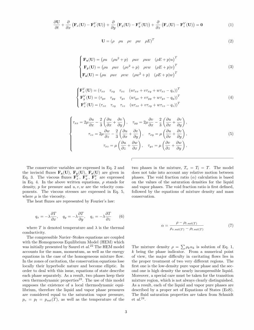
The experiments were conducted in a hydrodynamicloop of the DynFluid Laboratory fully described in a pre-vious work of Tomov et al.19. As a reminder, the loopconsists of two tanks of 150 L capacity each connected bycylindrical pipe with inner diameter of 40 mm. Betweenthe two tanks is placed the test section, represented inFig. 1, consisting in two transparent horizontally sym-metrical Venturi profiles with converging/diverging an-gles of 18◦ and 8◦, respectively.
The throat height is Hthroat = 10 mm and the width isconstant all along the test section and is equal to 10 mm.
FIG. 1. Venturi nozzle geometry at scale
In the present study, lengths are expressed with non-dimensional values X? = x
Hthroatwhereas the Reynolds
is defined at the Venturi throat with Hthroat and the ref-erence velocity Vref = 12 m.s−1 corresponding to themean velocity at the throat section, since it is the placewhere the flow regime changes its nature. The experi-
mental cavitation number is defined as σ =(Pref−Pvap)
12ρV
2ref
where Pref is measured at X? = −6 from the inlet of theVenturi section. The value of σ is corrected removing3% in order to take into account the real pressure at thethroat. One can refers to the precedent study of Tomovet al.19 for further information about the experimentalset-up characteristics and the uncertainties of measure-ments. It is difficult to perfectly match the experimentaland numerical values of the cavitation number. As aresult, the pressure at the outlet section of the Venturinozzle Pout is also expressed for numerical simulationssuch as the work of Schnerr et al.20.
Clearly visible peaks in a frequency spectrum are gen-erally related to spatial structures, which dispose withsome characteristic dimension. The issue of universal def-inition of a Strouhal number in cavitation is not straight-forward. It has been addressed, discussed and a proposalfor its unification has been given by Dular et al.21. In thepresent paper, the choice is made to define the Strouhalnumber as St = fHthroat
Vrefwith f corresponding to a fre-
quency of occurrence of a shedding feature.
B. Numerical modeling
1. Physical Model
The cavitating flows involve a very large variety ofphysical phenomena with different spatial and temporalscales. Typical examples are bubble or cloud vapor dy-namics and non-equilibrium thermodynamics. As a re-sult, it is difficult to fully resolve all scales, neverthelessthe current state of the art of the computers. Therefore,the modeling of each phase (liquid, vapor or mixture)present in the multiphase cavitating flow is of crucial im-portance for the good representation of the physics of theflow.
The compressible Navier - Stokes equations written incartesian coordinates without a source terms are given intheir conservative form in Eq. 1.
2
∂U
∂t+
∂
∂x
(Fx(U)− FVx (U)
)+
∂
∂y
(Fy(U)− FVy (U)
)+
∂
∂z
(Fz(U)− FVz (U)
)= 0 (1)
U = (ρ ρu ρv ρw ρE)T
(2)
Fx(U) =
(ρu (ρu2 + p) ρuv ρuw (ρE + p)u
)TFy(U) =
(ρu ρuv (ρv2 + p) ρvw (ρE + p)v
)TFz(U) =
(ρu ρuv ρvw (ρw2 + p) (ρE + p)w
)T (3)
FVx (U) = (τxx τxy τxz (uτxx + vτxy + wτxz − qx))
T
FVy (U) = (τyx τyy τyz (uτyx + vτyy + wτyz − qy))T
FVz (U) = (τzx τzy τzz (uτzx + vτzy + wτzz − qz))T(4)
τxx = 2µ∂u
∂x− 2
3
(∂u
∂x+∂v
∂y
), τyy = 2µ
∂v
∂x− 2
3
(∂u
∂x+∂v
∂y
),
τzz = 2µ∂w
∂z− 2
3
(∂u
∂x+∂v
∂y
), τxy = µ
(∂u
∂x+∂v
∂y
),
τxz = µ
(∂u
∂z+∂w
∂x
), τyz = µ
(∂v
∂z+∂w
∂y
),
(5)
The conservative variables are expressed in Eq. 2 andthe inviscid fluxes Fx(U), Fy(U), Fz(U) are given inEq. 3. The viscous fluxes FVx , FVy , FVz are expressedin Eq. 4. In the above written equations, ρ stands fordensity, p for pressure and u, v, w are the velocity com-ponents. The viscous stresses are expressed in Eq. 5,where µ is the viscosity.
The heat fluxes are represented by Fourier’s law:
qx = −λ∂T∂x
, qy = −λ∂T∂y
, qz = −λ∂T∂z
(6)
where T is denoted temperature and λ is the thermalconductivity.
The compressible Navier–Stokes equations are coupledwith the Homogeneous Equilibrium Model (HEM) whichwas initially presented by Saurel et al.22 The HEM modelaccounts for the mass, momentum, as well as the energyequations in the case of the homogeneous mixture flow.In the zones of cavitation, the conservation equations loselocally their hyperbolic nature and become elliptic. Inorder to deal with this issue, equations of state describeeach phase separately. As a result, two phases keep theirown thermodynamic properties23. The use of this modelsupposes the existence of a local thermodynamic equi-librium, therefore the liquid and vapor phase pressuresare considered equal to the saturation vapor pressure,pv = pl = psat(T ), as well as the temperature of the
two phases in the mixture, Tv = Tl = T . The modeldoes not take into account any relative motion betweenphases. The void fraction ratio (α) calculation is basedon the values of the saturation densities for the liquidand vapor phases. The void fraction ratio is first defined,followed by the equations of mixture density and massconservation.
α =ρ− ρl.sat(T )
ρv.sat(T ) − ρl.sat(T )(7)
The mixture density ρ =∑ρkαk is solution of Eq. 1,
k being the phase indicator. From a numerical pointof view, the major difficulty in cavitating flows lies inthe proper treatment of two very different regions. Thefirst one is the low-density pure vapor phase and the sec-ond one is high density the nearly incompressible liquid.Moreover, a special care must be taken for the transitionmixture region, which is not always clearly distinguished.As a result, each of the liquid and vapor pure phases aredescribed by a proper set of Equations of States (EoS).The fluid saturation properties are taken from Schmidtet al.24.
3
2. Conservation system closure - Phases EoS
EoS liquid phase
The liquid phase is firstly described with EoS. Thepressure of the liquid phase is governed by the modifiedTait equation of state, where K0 and N are constants22.The formulation considers the liquid phase as a saturatedcomponent of the multiphase flow.
p = K0
[(ρ
ρl,sat(T )
)N− 1
]+ Psat(T ) (8)
Where K0 = 3.3 × 10⁸ Pa and N = 7.15 for water.The temperature relation can be expressed in terms ofthe specific energy T = e−el0
Cvl+ T0, e being internal en-
ergy, el0 = 617 J.kg−1 is internal energy at referencetemperature T0 = 273.15 K and Cvl = 4180 J.kg−1.K−1
is the liquid specific heat at constant volume. Vogel–Fulcher–Tammann’s law25–27 gives the dynamic viscosityformulation:
µl = A× 10B/(T−C) (9)
In the case of water A = 2.414 × 10⁻⁵ Pa.s, B = 247.8K and C = 140.0 K. Thermal conductivity of water isconsidered constant and it is taken λl = 0.6 W.m−1.K−1.
The formulation of the speed of sound is derived fromthe hypothesis that the acoustic pressure fluctuations canbe neglected in comparison with the cavitation pressure.Equation 10 gives the speed of sound in pure liquid. Moreinformation about its derivation is given in Appendix A.
c2l =N(p− psat(T ) +K0)
ρ+
p
ρ2Cvl
(∂psat(T )
∂T− N(p− psat(T ) +K0)
ρl,sat(T )
∂ρsat(T )
∂T
)(10)
EoS vapor phase
The EoS for the vapor phase are described below. Themain hypothesis behind the vapor phase is its consid-eration as a perfect gas, hence the following relation isapplied:
p = (γ − 1) ρe (11)
The temperature equation is written in terms of thelatent heat of vaporization Lv(T0) = 2.753 × 10⁶ J.kg−1
at temperature T0 = 273.15 K as T = e−el0−Lv(T0)Cvv
+ T0,
Cvv = 1410.8 J.kg−1.K−1 being vapor specific heat at
constant volume. The dynamic viscosity formulation isgiven by Sutherland’s28 law.
µv = µref
(T
Tref
)3/2Tref + S
T + S(12)
Sutherland’s constants for water are: µref = 18.27 ×10⁻³ Pa.s, Tref = 291.15 K, S = 861.11 K. The thermalconductivity of vapor is a function of temperature and isgiven by Dincer et al.29 as follows:
λv =
4∑i=0
aiTi (13)
where a0 = −7.967996 × 10⁻³, a1 = 6.881332 × 10⁻⁵,a2 = 4.49046 × 10⁻⁸, a3 = −9.099937 × 10⁻¹², a4 =6.173314× 10⁻¹⁶.
Since the vapor is treated as a perfect gas, the speedof sound is given by the known relation:
c2v =γp
ρ(14)
where γ = 1.327 for water vapor, ρ and p are solutionof Eq. 1.
Mixture closure equations and phase transition
As mentioned above, the basic hypothesis is that thefluid is in a local thermodynamic equilibrium, hence, atthe mixture zone the pressure and temperatures are thesame for each phases. To manage mass transfers betweenphases and therefore the choose of EoS of each phase tocompute temperature, pressure and the other thermody-namics properties, an explicit phase transition algorithmbased on densities is used. It starts by considering allthe variables at the previous time step given by solvingEq. 1, if density is lower than the vapor saturation den-sity then the phase is pure vapor, α = 1, EoS of vaporis used. If density is higher than liquid saturation den-sity then the phase is pure liquid, α = 0, modified TaitEoS is used. And finally, if density is between the twophases saturation densities then α is given by Eq. 7 andtemperature is computed by solving e = εev + (1− ε)el, εbeing vapor mass fraction, the internal energies ev and elare given by EoS of vapor and liquid, respectively, givenabove. The phase transition algorithm is presented indetails in Appendix B. Since the next time step temper-ature is computed for each phase using the proceduredescribed above, other parameters can be derived suchas the mixture viscosity,
µm =1
εµv
+ 1−εµl
(15)
4

and mixture thermal conductivity λm which is com-puted the same way.
One of the advantages of the used approach is thatit takes into consideration the physical variations of thepressure since the compressibility of each phase is takeninto account. The EoS properly describe the physics ofeach phase and no modifications of the speed of soundare to be considered (no preconditioning issues are re-tained). This last point is crucial for the restitution ofthe real behavior of likely condensation shock waves de-scribed further in this paper. On the other hand, thespeed of sound drastically varies from phase to other andneed to be correctly modeled in the mixture phase. In-deed, the flow presents very low Mach numbers in thepure liquid phase, intermediate in the pure vapor phaseand is supersonic in the mixture phase, the sound veloc-ity being very low. In our case, it is expressed followingthe Wood’s relation30:
1
ρc2m=
α
ρv,sat(T )ρc2v+
1− αρl,sat(T )c2l
(16)
Equation 16 takes into consideration the phase transi-tion through the vapor fraction ratio α. The same for-mulation has been recently used by Saurel et al.31 in thecase of a cavitating boiling and evaporating flows.
3. Numerical framework
Finite volume solver: The used finite volume solveris based on Moving Least Squares32,33 (FV-MLS) ap-proximations. This approach is somewhat different thatthe usual approach of high-order (≥ 2) finite volumeschemes. The usual approach is pragmatic and “bottom-up” . Starting from an underlying piecewise constantrepresentation, a discontinuous reconstruction of the fieldvariables is performed at the cell level. The FV-MLSmethod starts from a high-order and highly regular rep-resentation of the solution, obtained by means of MovingLeast-Squares approximation, and it is well suited forgeneral, unstructured grids. This approach is directlysuitable for the discretization of elliptic/parabolic equa-tions and high order spatial terms. For equations with apredominantly hyperbolic character, the global represen-tation is broken locally, at the cell level, into a piecewisepolynomial reconstruction, which allows to use the pow-erful finite volume technology of Godunov-type schemes(e.g. Riemann solvers, limiters). A linear reconstructionis used implying a second order space accuracy in our caseassociated to a Vankatakrishnan slope limiter to manageshocks discontinuities induced by supersonic regimes (seethe following section). The reader is kindly referred toworks of Nogueira et al.33,34 and Khelladi et al.32 formore details concerning this numerical method.
Low Mach number handling: The disparities betweenthe values of speed of sound into the flow phases are
very high. Indeed, the speed of sound is approxima-tively equal to 1500 m.s−1 for the liquid (α = 0), 400m.s−1 for the vapor (α = 1) and around 4 m.s−1 in themixture (α = 0.5). As a result, the compressibility ef-fects based on the Mach number vary in respect to thezone of calculation. Therefore, this issue should be takeninto consideration when dealing with numerical flux atvery low and very high Mach number calculations. It iswidely known that it is difficult to solve the compressibleequations for very low Mach numbers using ”standard”numerical flux (Roe, Rusanov,...) due to the inducednumerical dissipation on the prediction of the pressure,p ∼ M rather than p ∼ M2. In addition, for an explicittime schemes this induces very small time steps (veryrestrictive CFL condition). Using preconditioning tech-niques35 may overcome these limitations, unfortunately,this implies to modify implicitly the pressure wave prop-agation dynamics (speed of sound) in the liquid phasewhich is not suitable in view of the demonstrations pro-jected in the following developments. Consequently, inthe present paper, the code does not use any precondi-tioning. In such a way the authors estimate that thecode simulates a better physical behavior of each of theflow phases. A drawback is the need of a very small timestep which in our case is around 10−7s using a first orderexplicit Euler time scheme31.
Approximate Riemann solver: As mentioned above,the finite volume solver should deal with a large rangeof wave propagation regimes due to the phase transi-tion mechanisms. The used approximate Riemann solvershould then be able to support all-speed regimes. A re-cent work done by Nogueira et al.36 demonstrates thatincreasing space order of accuracy to 4th or 5th space or-ders in addition to the use of a fix of the dissipation term(function of Mach number) of Roe or Rusanov approxi-mate Riemann solvers, for instance, may extend their useto all-speed regimes. For some pragmatic reasons relatedto the nature of the present investigation, the second or-der space of accuracy is estimated sufficient. For thisreason a modified Simple Low dissipative AUSM solver(SLAU) is used in the present case. The AUSM fam-ily solvers are based on the splitting of numerical fluxterm into convective and pure pressure one. The convec-tive part is decomposed following the procedure proposedby Shima et al37. The mathematical development is be-yond the scope of the present paper. For more details thereader is kindly referred to the work of Kitamura et al.38.
Turbulence handling: In general, a sub-grid scales(SGS) model in a Large-Eddy Simulation (LES) oper-ates on a range of scales that is resolved by discretiza-tion schemes. As a result of that, the truncation error ofthe scheme and the SGS model are mutually linked. Thenumerical approaches where SGS model and discretiza-tion scheme are merged, are called implicit LES (iLES)methods39. ILES approach is used in this work. Indeed,to highlight the targeted physical mechanisms related tocloud cavitation shedding and because of the propertiesof FV-MLS scheme, no turbulence model is used explic-
5
itly. Turbulence is taken implicitly into considerationthrough the definition of an adequate number of points inthe stencil and the use of appropriate MLS-kernel func-tion parameters in each spatial direction according toNogueira et al.34,40. A description of the choice of thebest values of stencil morphology and the best kernel pa-rameters are beyond the scope of this paper. For moredetails and explications, as well as benchmark results,one is kindly referred to references 32–34, and 40.
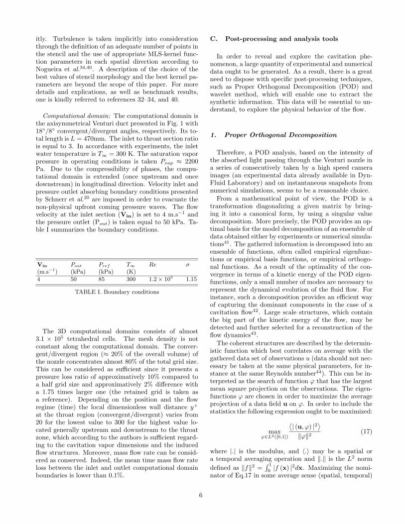
Computational domain: The computational domain isthe axisymmetrical Venturi duct presented in Fig. 1 with18◦/8◦ convergent/divergent angles, respectively. Its to-tal length is L = 470mm. The inlet to throat section ratiois equal to 3. In accordance with experiments, the inletwater temperature is T∞ = 300 K. The saturation vaporpressure in operating conditions is taken Pvap ≈ 2200Pa. Due to the compressibility of phases, the compu-tational domain is extended (once upstream and oncedownstream) in longitudinal direction. Velocity inlet andpressure outlet absorbing boundary conditions presentedby Schnerr et al.20 are imposed in order to evacuate thenon-physical upfront coming pressure waves. The flowvelocity at the inlet section (Vin) is set to 4 m.s−1 andthe pressure outlet (Pout) is taken equal to 50 kPa. Ta-ble I summarizes the boundary conditions.
Vin Pout Pref T∞ Re σ(m.s−1) (kPa) (kPa) (K)4 50 85 300 1.2× 10⁵ 1.15
TABLE I. Boundary conditions
The 3D computational domains consists of almost3.1 × 105 tetrahedral cells. The mesh density is notconstant along the computational domain. The conver-gent/divergent region (≈ 20% of the overall volume) ofthe nozzle concentrates almost 80% of the total grid size.This can be considered as sufficient since it presents apressure loss ratio of approximatively 10% compared toa half grid size and approximatively 2% difference witha 1.75 times larger one (the retained grid is taken asa reference). Depending on the position and the flowregime (time) the local dimensionless wall distance y+
at the throat region (convergent/divergent) varies from20 for the lowest value to 300 for the highest value lo-cated generally upstream and downstream to the throatzone, which according to the authors is sufficient regard-ing to the cavitation vapor dimensions and the inducedflow structures. Moreover, mass flow rate can be consid-ered as conserved. Indeed, the mean time mass flow rateloss between the inlet and outlet computational domainboundaries is lower than 0.1%.
C. Post-processing and analysis tools
In order to reveal and explore the cavitation phe-nomenon, a large quantity of experimental and numericaldata ought to be generated. As a result, there is a greatneed to dispose with specific post-processing techniques,such as Proper Orthogonal Decomposition (POD) andwavelet method, which will enable one to extract thesynthetic information. This data will be essential to un-derstand, to explore the physical behavior of the flow.
1. Proper Orthogonal Decomposition
Therefore, a POD analysis, based on the intensity ofthe absorbed light passing through the Venturi nozzle ina series of consecutively taken by a high speed cameraimages (an experimental data already available in Dyn-Fluid Laboratory) and on instantaneous snapshots fromnumerical simulations, seems to be a reasonable choice.
From a mathematical point of view, the POD is atransformation diagonalizing a given matrix by bring-ing it into a canonical form, by using a singular valuedecomposition. More precisely, the POD provides an op-timal basis for the model decomposition of an ensemble ofdata obtained either by experiments or numerical simula-tions41. The gathered information is decomposed into anensemble of functions, often called empirical eigenfunc-tions or empirical basis functions, or empirical orthogo-nal functions. As a result of the optimality of the con-vergence in terms of a kinetic energy of the POD eigen-functions, only a small number of modes are necessary torepresent the dynamical evolution of the fluid flow. Forinstance, such a decomposition provides an efficient wayof capturing the dominant components in the case of acavitation flow42. Large scale structures, which containthe big part of the kinetic energy of the flow, may bedetected and further selected for a reconstruction of theflow dynamics43.
The coherent structures are described by the determin-istic function which best correlates on average with thegathered data set of observations u (data should not nec-essary be taken at the same physical parameters, for in-stance at the same Reynolds number44). This can be in-terpreted as the search of function ϕ that has the largestmean square projection on the observations. The eigen-functions ϕ are chosen in order to maximize the averageprojection of a data field u on ϕ. In order to include thestatistics the following expression ought to be maximized:
maxϕ∈L2([0,1])
⟨| (u, ϕ) |2
⟩‖ϕ‖2
(17)
where |.| is the modulus, and 〈.〉 may be a spatial ora temporal averaging operation and ‖.‖ is the L2 norm
defined as ‖f‖2 =∫ 1
0|f (x) |2dx. Maximizing the nomi-
nator of Eq.17 in some average sense (spatial, temporal)
6
while keeping the constraint ‖ϕ‖2 = 1 leads to the func-tional:
J [ϕ] =⟨‖ (u, ϕ) ‖2
⟩− λ
(‖ϕ‖2 − 1
)(18)
The choice of the average operator is crucial for the ap-plication of the POD analysis. The upper functional istrue for all variations ϕ+ δψ ∈ L2, δψ ∈ R:
d
dδJ [ϕ+ δψ] |δ=0 = 0. (19)
We can then obtain the integral equation of Fredholm:∫ 1
0
〈u (x)u∗ (x′)〉ϕ (x′) dx′ = λϕ (x) . (20)
For more details about the full mathematical develop-ment, one is kindly referred to the PhD thesis of Bren-ner45. The eigenfunctions {ϕj} produce the optimal ba-sis derived from Eq. 20 using the averaged autocorrela-tion function R (x, x′) = 〈u (x)u∗ (x′)〉. According to theHilbert theory, one can assume there is an infinity of or-thogonal eigenfunctions associated to the eigenvalues, asa result of the diagonal decomposition of the autocorre-lation function. Since the averaged autocorrelation func-tion is R(x, x
′) ≥ 0, and Eq. 17 admits a solution equal to
the largest eigenvalue of the problem, the eigenvalues λjtake the following order λj ≥ λj+1 ≥ 0. Each data field umay be reconstructed by using the modal decomposition
of eigenfunctions ϕj , as u (x) =∞∑j=1
ajϕj (x), where aj is
a reconstruction coefficient defined as 〈aja∗k〉 = δjkλj . Inthe case where one has information regarding the velocityfield, the eigenvalues represent twice the average kineticenergy of each mode ϕj . In such a way, the first eigenval-ues correspond to the most energetic modes, hence themost energetic structures. In order to improve the post-processing algorithm and computational time, a snapshotPOD method has been used by Sirovich46. In the classi-cal POD method , the operator 〈.〉 stands for a temporal
average and R(x, x′) stands for a spatial correlation ten-
sor. The use of a snapshot POD makes the size of theeigenvalue problem to be equal to the number of treatedimages N using 〈.〉 as a spatial average and a two-point
temporal correlation one C(t, t′) instead of the spatial
correlation in the classic method. In a general manner,when the number of spatial points of data is much greaterthan the number of treated images, the snapshot PODreduces considerably the necessary computational timefor post-processing. As a result, in the present study, thesnapshot POD approach will be preferred.
2. Wavelet Method Analysis
Wavelet analysis is usually used to decompose timesignals into time-frequency space allowing to determinedominant modes of variability through time and, as a re-sult, to associate a dynamic phenomenon to his frequency
of occurrence. This method, mainly used in geophysicsstudies, is particularly adapted to detect near-periodicphenomena as cloud cavitation shedding.
This method, more powerful than classical signalanalysis method such as Windowed Fourrier Transform(WTF), has the advantage to be relatively accurate intime frequency localization and also scale independent.Kjeldsen et al.47 are the first to propose the wavelet anal-ysis as a relevant method to measure shedding mecha-nisms. Brandner et al.48 performed a wavelet analysisin order to extract frequencies of cloud cavitation shed-ding from a cavity induced by a jet in a cross-flow. In thepresent paper, the wavelet method developed by Torrenceet al.49 is applied to extract the frequencies of appear-ance of two cloud shedding phenomena which can occursimultaneity. A quick presentation of the method appliedto image analysis is developed thereafter.
The method is based on a continuous non-orthogonalwavelet function Ψ0 which is used in order to performa complex wavelet transform Wn on a signal scalar seriexn. After normalization, Wn can be expressed as:
Wn(s) =
N−1∑n′=0
xn′
√δt
sΨ∗0
[(n′ − n)δt
s
](21)
where s is the wavelet scale, which determine themethod precision, δt is the time between two images, Nis the number of images and (∗) indicates the complexconjugate.
The choice of the function Ψ0 is here of primordialimportance and might be adapted to the study. In thecase of image analysis, where the main goal is to extractfrequencies of occurrence of some phenomena, a Mor-let 6 function is usually used6,48,49. The Morlet base,which represents a plane wave modulated by a Gaussian(Fig. 2), is expressed in the time domain analytically asa function Ψ0 of η, the non-dimensional time,
Ψ0(η) = π−1/4eiω0ηe−η2/2 (22)
whereas the associated function in the frequency do-main, obtained by the Fourrier transform of Ψ0, can bewritten as a function of the frequency ω:
Ψ0(sω) = π−1/4H(ω)e−(sω−ω0)2/2 (23)
where ω0 is a non-dimensional frequency constant(taken to be 6 for Morlet base49) and H(ω) is a heavisidestep function. Both functions are represented below infigure 2.
As a result, using the discrete Fourier transform xk ofthe discrete sequence of images xn (where k = 0...N − 1is the frequency index) and based on equation 21 and 23,the wavelet transform can be written in Fourrier space:
Wn(s) =
N−1∑k=0
xk
√2πs
δtΨ∗0(sωk)eiωkδt (24)
7
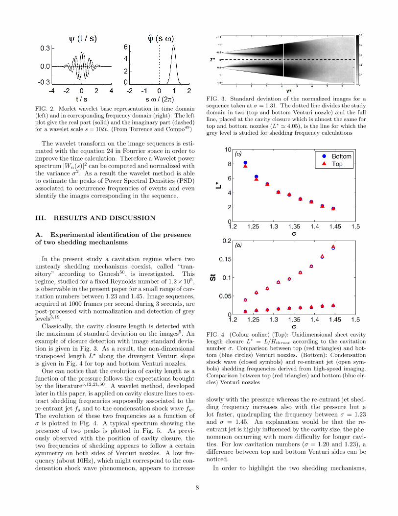
FIG. 2. Morlet wavelet base representation in time domain(left) and in corresponding frequency domain (right). The leftplot give the real part (solid) and the imaginary part (dashed)for a wavelet scale s = 10δt. (From Torrence and Compo49)
The wavelet transform on the image sequences is esti-mated with the equation 24 in Fourrier space in order toimprove the time calculation. Therefore a Wavelet powerspectrum |Wn(s)|2 can be computed and normalized withthe variance σ2. As a result the wavelet method is ableto estimate the peaks of Power Spectral Densities (PSD)associated to occurrence frequencies of events and evenidentify the images corresponding in the sequence.
III. RESULTS AND DISCUSSION
A. Experimental identification of the presenceof two shedding mechanisms
In the present study a cavitation regime where twounsteady shedding mechanisms coexist, called “tran-sitory” according to Ganesh50, is investigated. Thisregime, studied for a fixed Reynolds number of 1.2×10⁵,is observable in the present paper for a small range of cav-itation numbers between 1.23 and 1.45. Image sequences,acquired at 1000 frames per second during 3 seconds, arepost-processed with normalization and detection of greylevels5,19.
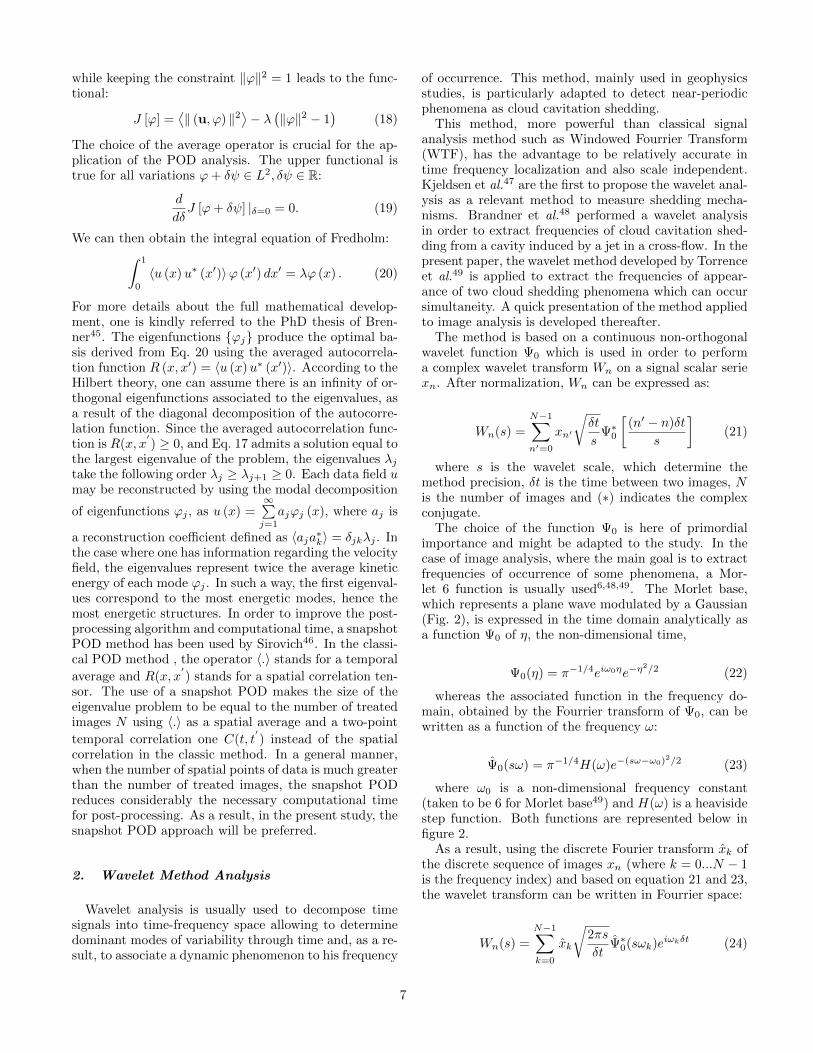
Classically, the cavity closure length is detected withthe maximum of standard deviation on the images5. Anexample of closure detection with image standard devia-tion is given in Fig. 3. As a result, the non-dimensionaltransposed length L? along the divergent Venturi slopeis given in Fig. 4 for top and bottom Venturi nozzles.
One can notice that the evolution of cavity length as afunction of the pressure follows the expectations broughtby the literature5,12,21,50. A wavelet method, developedlater in this paper, is applied on cavity closure lines to ex-tract shedding frequencies supposedly associated to there-entrant jet fs and to the condensation shock wave fw.The evolution of these two frequencies as a function ofσ is plotted in Fig. 4. A typical spectrum showing thepresence of two peaks is plotted in Fig. 5. As previ-ously observed with the position of cavity closure, thetwo frequencies of shedding appears to follow a certainsymmetry on both sides of Venturi nozzles. A low fre-quency (about 10Hz), which might correspond to the con-densation shock wave phenomenon, appears to increase
FIG. 3. Standard deviation of the normalized images for asequence taken at σ = 1.31. The dotted line divides the studydomain in two (top and bottom Venturi nozzle) and the fullline, placed at the cavity closure which is almost the same fortop and bottom nozzles (L? ' 4.05), is the line for which thegrey level is studied for shedding frequency calculations
FIG. 4. (Colour online) (Top): Unidimensional sheet cavitylength closure L? = L/Hthroat according to the cavitationnumber σ. Comparison between top (red triangles) and bot-tom (blue circles) Venturi nozzles. (Bottom): Condensationshock wave (closed symbols) and re-entrant jet (open sym-bols) shedding frequencies derived from high-speed imaging.Comparison between top (red triangles) and bottom (blue cir-cles) Venturi nozzles
slowly with the pressure whereas the re-entrant jet shed-ding frequency increases also with the pressure but alot faster, quadrupling the frequency between σ = 1.23and σ = 1.45. An explanation would be that the re-entrant jet is highly influenced by the cavity size, the phe-nomenon occurring with more difficulty for longer cavi-ties. For low cavitation numbers (σ = 1.20 and 1.23), adifference between top and bottom Venturi sides can benoticed.
In order to highlight the two shedding mechanisms,
8
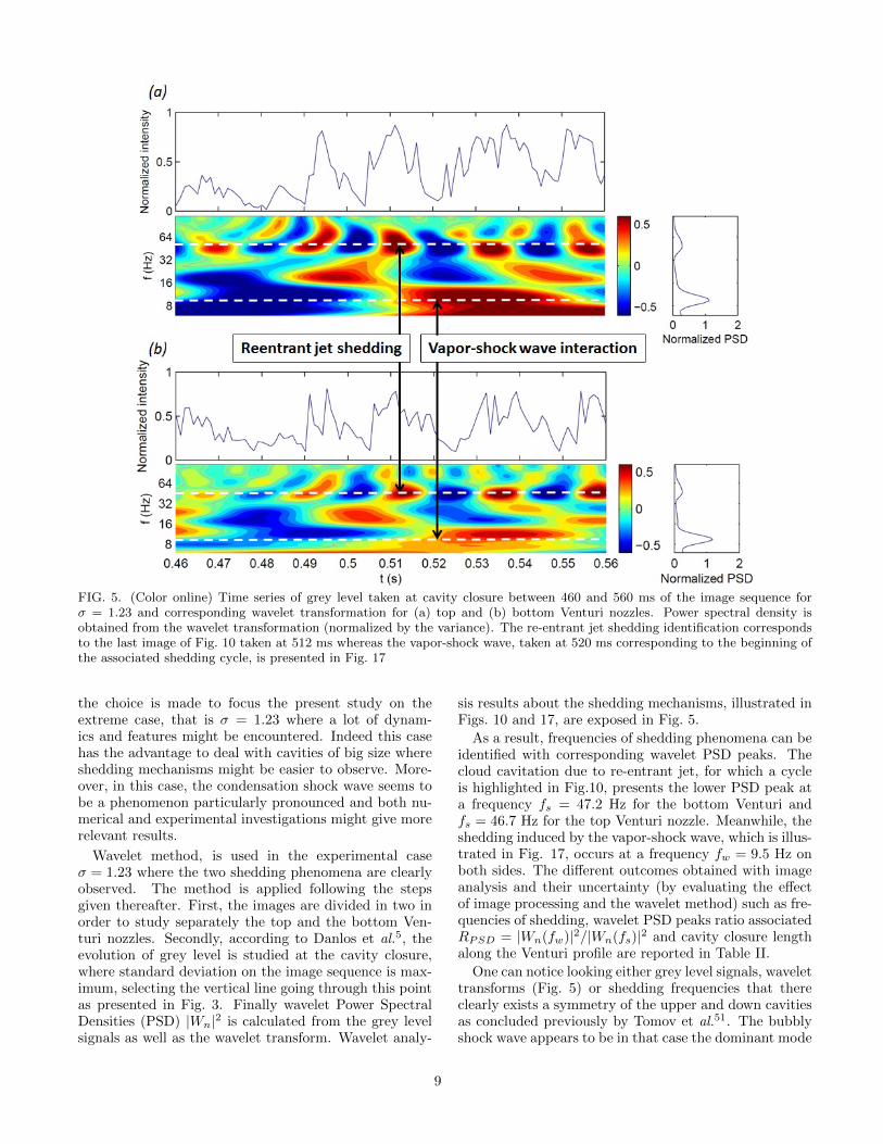
FIG. 5. (Color online) Time series of grey level taken at cavity closure between 460 and 560 ms of the image sequence forσ = 1.23 and corresponding wavelet transformation for (a) top and (b) bottom Venturi nozzles. Power spectral density isobtained from the wavelet transformation (normalized by the variance). The re-entrant jet shedding identification correspondsto the last image of Fig. 10 taken at 512 ms whereas the vapor-shock wave, taken at 520 ms corresponding to the beginning ofthe associated shedding cycle, is presented in Fig. 17
the choice is made to focus the present study on theextreme case, that is σ = 1.23 where a lot of dynam-ics and features might be encountered. Indeed this casehas the advantage to deal with cavities of big size whereshedding mechanisms might be easier to observe. More-over, in this case, the condensation shock wave seems tobe a phenomenon particularly pronounced and both nu-merical and experimental investigations might give morerelevant results.
Wavelet method, is used in the experimental caseσ = 1.23 where the two shedding phenomena are clearlyobserved. The method is applied following the stepsgiven thereafter. First, the images are divided in two inorder to study separately the top and the bottom Ven-turi nozzles. Secondly, according to Danlos et al.5, theevolution of grey level is studied at the cavity closure,where standard deviation on the image sequence is max-imum, selecting the vertical line going through this pointas presented in Fig. 3. Finally wavelet Power SpectralDensities (PSD) |Wn|2 is calculated from the grey levelsignals as well as the wavelet transform. Wavelet analy-
sis results about the shedding mechanisms, illustrated inFigs. 10 and 17, are exposed in Fig. 5.
As a result, frequencies of shedding phenomena can beidentified with corresponding wavelet PSD peaks. Thecloud cavitation due to re-entrant jet, for which a cycleis highlighted in Fig.10, presents the lower PSD peak ata frequency fs = 47.2 Hz for the bottom Venturi andfs = 46.7 Hz for the top Venturi nozzle. Meanwhile, theshedding induced by the vapor-shock wave, which is illus-trated in Fig. 17, occurs at a frequency fw = 9.5 Hz onboth sides. The different outcomes obtained with imageanalysis and their uncertainty (by evaluating the effectof image processing and the wavelet method) such as fre-quencies of shedding, wavelet PSD peaks ratio associatedRPSD = |Wn(fw)|2/|Wn(fs)|2 and cavity closure lengthalong the Venturi profile are reported in Table II.
One can notice looking either grey level signals, wavelettransforms (Fig. 5) or shedding frequencies that thereclearly exists a symmetry of the upper and down cavitiesas concluded previously by Tomov et al.51. The bubblyshock wave appears to be in that case the dominant mode
9
of cloud shedding in comparison with the re-entrant jet.However in this particular case, where cavities are longenough, the symmetry seems to begin to break. Indeed,as previously noticed, a difference between top and bot-tom Venturi cavity lengths and re-entrant jet frequenciescan be seen. The 2D observations do not permit to in-terpret this symmetry break-up. On the other hand, 3Dsimulations could reveal such a dynamical feature.
B. Comparison of global features with PODtechniques
This section presents the application of the POD onseries of vapor fraction consecutive images taken fromthe numerical simulations. The POD is used as a com-plementary technique to study the different cavitationregimes. The side view images are taken at three differ-ent equally spaced locations on the Venturi nozzle: thefront, the middle and the back. For each location a totalnumber of 1200 images are extracted. By definition, theoptimal basis is given by the eigenfunctions ϕj of Eq. 20.In the present study u(x) is the vapor fraction, hence theeigenfunctions ϕj play the role of a “weight” for the re-construction of the flow. Moreover, if u(x) represents avelocity field, ϕj would have been a kinetic energy.
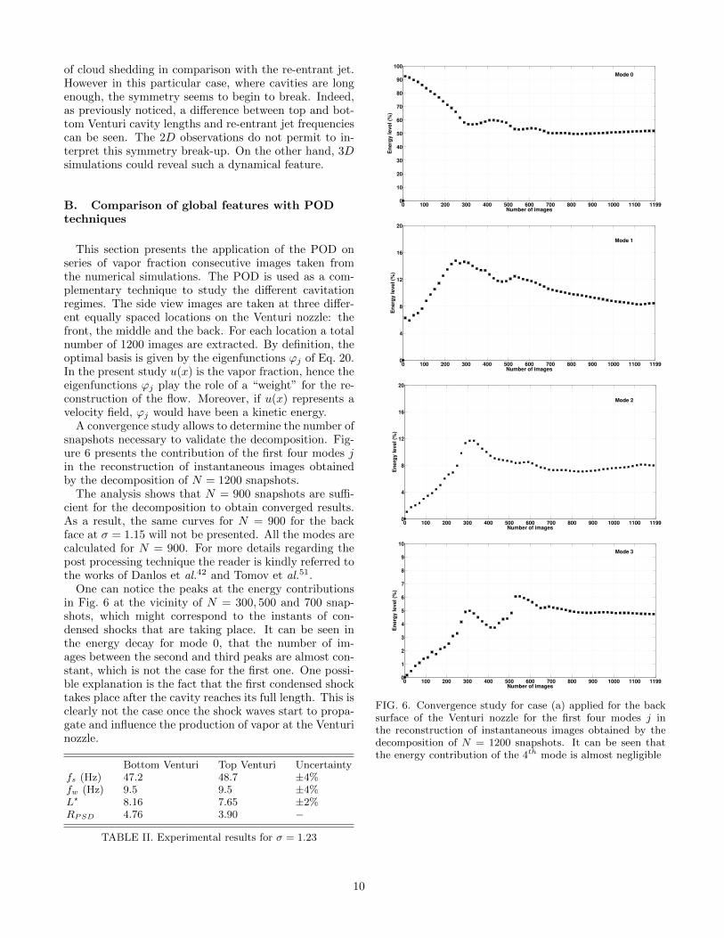
A convergence study allows to determine the number ofsnapshots necessary to validate the decomposition. Fig-ure 6 presents the contribution of the first four modes jin the reconstruction of instantaneous images obtainedby the decomposition of N = 1200 snapshots.
The analysis shows that N = 900 snapshots are suffi-cient for the decomposition to obtain converged results.As a result, the same curves for N = 900 for the backface at σ = 1.15 will not be presented. All the modes arecalculated for N = 900. For more details regarding thepost processing technique the reader is kindly referred tothe works of Danlos et al.42 and Tomov et al.51.
One can notice the peaks at the energy contributionsin Fig. 6 at the vicinity of N = 300, 500 and 700 snap-shots, which might correspond to the instants of con-densed shocks that are taking place. It can be seen inthe energy decay for mode 0, that the number of im-ages between the second and third peaks are almost con-stant, which is not the case for the first one. One possi-ble explanation is the fact that the first condensed shocktakes place after the cavity reaches its full length. This isclearly not the case once the shock waves start to propa-gate and influence the production of vapor at the Venturinozzle.
Bottom Venturi Top Venturi Uncertaintyfs (Hz) 47.2 48.7 ±4%fw (Hz) 9.5 9.5 ±4%L? 8.16 7.65 ±2%RPSD 4.76 3.90 −
TABLE II. Experimental results for σ = 1.23
0 100 200 300 400 500 600 700 800 900 1000 1100 11990
10
20
30
40
50
60
70
80
90
100
Number of images
En
erg
y level (%
)
Mode 0
0 100 200 300 400 500 600 700 800 900 1000 1100 11990
4
8
12
16
20
Number of images
En
erg
y level (%
)
Mode 1
0 100 200 300 400 500 600 700 800 900 1000 1100 11990
4
8
12
16
20
Number of images
En
erg
y l
ev
el
(%)
Mode 2
0 100 200 300 400 500 600 700 800 900 1000 1100 11990
1
2
3
4
5
6
7
8
9
10
Number of images
En
erg
y l
ev
el
(%)
Mode 3
FIG. 6. Convergence study for case (a) applied for the backsurface of the Venturi nozzle for the first four modes j inthe reconstruction of instantaneous images obtained by thedecomposition of N = 1200 snapshots. It can be seen thatthe energy contribution of the 4th mode is almost negligible
10

FIG. 7. (Color online) (Left): POD on side view images atsuperimposed numerical data, (Right): POD on side viewimages from experimental data
In order to compare the experimental and numericalPOD modes, one would need to deal with superimposedside view numerical snapshots, nevertheless the relativelysmall number of cavitation cycles data gathered from thesimulations. According to the authors, the vapor struc-tures may not necessarily lay in the same spatial plane,as it is the case in experimental side views.
As a result, Fig. 7 illustrates POD modes of numeri-cally superimposed snapshots and experimental ones. Itcan be observed that the lengths of the cavitation va-por are comparable for modes 0. Moreover, the advectedvapor structures are symmetrically spread for both cou-ples of modes 1 and 2. One can notice the likelihoodfor the vapor characteristic length to be in the range of6Hthroat to 7Hthroat for the numerical case and 7Hthroat
to 8Hthroat for the experimental one.In order to take into consideration the possible 3D ef-
fects, the first four modes extracted from numerical dataare presented in Fig. 8 for σ = 1.15. The values of theenergy contributions per mode and per plane are givenin Table III. It can be seen that the values per modeare comparable for all of the cases. A brief discussionabout the POD application on numerical data is firstlyprovided, followed by a discussion on the experimentalPOD modes.
The energy contributions of the first four numericalmodes contribute to almost 100%, as it can be seen fromTable III. For each plane, modes 0 account for slightly
FIG. 8. (Color online) The first four numerical modes foreach plane location at σ = 1.15. The dashed line representsthe horizontal line of symmetry
Plane Mode 0 Mode 1 Mode 2 Mode 3 TotalFront 90.71 7.65 1.21 0.24 99.84Middle 92.50 6.19 0.94 0.19 99.82Rear 92.38 6.29 1.05 0.17 99.89Experiment 89.45 5.75 1.45 0.30 96.95
TABLE III. Energy contributions per mode [%]
11
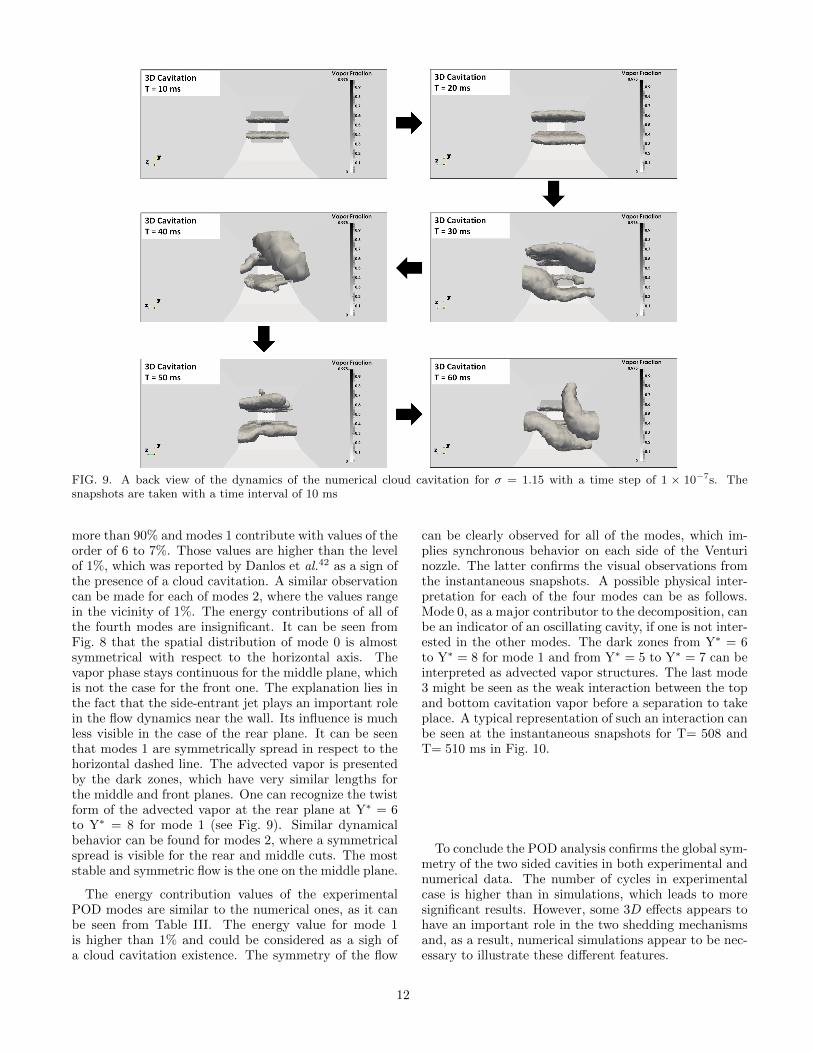
FIG. 9. A back view of the dynamics of the numerical cloud cavitation for σ = 1.15 with a time step of 1 × 10⁻⁷s. Thesnapshots are taken with a time interval of 10 ms
more than 90% and modes 1 contribute with values of theorder of 6 to 7%. Those values are higher than the levelof 1%, which was reported by Danlos et al.42 as a sign ofthe presence of a cloud cavitation. A similar observationcan be made for each of modes 2, where the values rangein the vicinity of 1%. The energy contributions of all ofthe fourth modes are insignificant. It can be seen fromFig. 8 that the spatial distribution of mode 0 is almostsymmetrical with respect to the horizontal axis. Thevapor phase stays continuous for the middle plane, whichis not the case for the front one. The explanation lies inthe fact that the side-entrant jet plays an important rolein the flow dynamics near the wall. Its influence is muchless visible in the case of the rear plane. It can be seenthat modes 1 are symmetrically spread in respect to thehorizontal dashed line. The advected vapor is presentedby the dark zones, which have very similar lengths forthe middle and front planes. One can recognize the twistform of the advected vapor at the rear plane at Y∗ = 6to Y∗ = 8 for mode 1 (see Fig. 9). Similar dynamicalbehavior can be found for modes 2, where a symmetricalspread is visible for the rear and middle cuts. The moststable and symmetric flow is the one on the middle plane.
The energy contribution values of the experimentalPOD modes are similar to the numerical ones, as it canbe seen from Table III. The energy value for mode 1is higher than 1% and could be considered as a sigh ofa cloud cavitation existence. The symmetry of the flow
can be clearly observed for all of the modes, which im-plies synchronous behavior on each side of the Venturinozzle. The latter confirms the visual observations fromthe instantaneous snapshots. A possible physical inter-pretation for each of the four modes can be as follows.Mode 0, as a major contributor to the decomposition, canbe an indicator of an oscillating cavity, if one is not inter-ested in the other modes. The dark zones from Y∗ = 6to Y∗ = 8 for mode 1 and from Y∗ = 5 to Y∗ = 7 can beinterpreted as advected vapor structures. The last mode3 might be seen as the weak interaction between the topand bottom cavitation vapor before a separation to takeplace. A typical representation of such an interaction canbe seen at the instantaneous snapshots for T= 508 andT= 510 ms in Fig. 10.
To conclude the POD analysis confirms the global sym-metry of the two sided cavities in both experimental andnumerical data. The number of cycles in experimentalcase is higher than in simulations, which leads to moresignificant results. However, some 3D effects appears tohave an important role in the two shedding mechanismsand, as a result, numerical simulations appear to be nec-essary to illustrate these different features.
12

FIG. 10. Normalized instantaneous snapshots from high-speed image series showing the re-entrant jet dynamics for σ = 1.23.The images are taken in the total sequence between 498 and 512 ms with ∆t = 2 ms. The horizontal symmetry is shown inwhite dashed line. The re-entrant jet appears at the same instant on the top and bottom side of the nozzle. It flows upstreamthe flow, while creating recirculating vapor zones and a hairpin vortex. It is then advected by the flow and a vapor separationtakes place
C. Re-entrant jet shedding
As previously explained in Sec. II, the re-entrant jetis a well known shedding mechanism observed9,10,15 andcharacterized5,12,50 in several studies. The cycle illus-trated in Fig. 10 consists of the following steps: first, thecavity grows from the Venturi throat and a re-entrant jetappears at the sheet cavity closure. Secondly, it flows
upstream on the wall and eventually cuts the formed va-por. In general, the re-entrant jet is created by the flowby an expansion of its closure region. In such a wayand in a combination with the Venturi wall, a stagnationpoint is created. The conservation of momentum makesthe fluid to pass beneath the cavity, hence the jet pro-gresses and results in a vapor separation52. As a result,a cloud is formed and is further advected. The cloud va-
13
por collapses in the divergent Venturi nozzle zone wherethe pressure is higher than the one at the throat sec-tion. In such a way, the cavity length is reduced andthe whole process repeats itself. The repeatability of theprocess is characterized by the shedding frequency fs. Inthe present section, the re-entrant jet shedding dynam-ics are pointed out with wavelet grey level analysis (seeFig. 5). Afterwards, the numerical simulations are in-troduced and a comparison is made with experimentaldata.
Figure 10 shows the multiphase flow dynamics in ex-perimental conditions for σ = 1.23. A sequence of nor-malized instantaneous snapshots in Fig. 10 are presentedin order to illustrate the re-entrant jet dynamics. Its de-velopment can be seen at the closure region on both sidesof the nozzle. The re-entrant jet travels upstream theflow and it creates two recirculating vapor zones. Fur-thermore, one can see the clouds cavitation expansionand the creation of a hairpin vortex. It plays the roleof an interaction between the top and bottom divergentsides of the nozzle. The re-entrant jet continues to travelupstream, while the hairpin vortex is advected by theflow until vapor separation. The wavelet transform as-sociated to the sequence (Fig. 5) show that the vaporseparation occurring at 512 ms correspond to a peak ofwavelet power spectrum for both Venturi nozzles at afrequency fs ' 48 Hz (see Table II). As a result, there-entrant jet dynamic is well-characterized experimen-tally in two dimension with a frequency of occurrence fs,however numerical simulations are required in order tosee possible 3D effects.
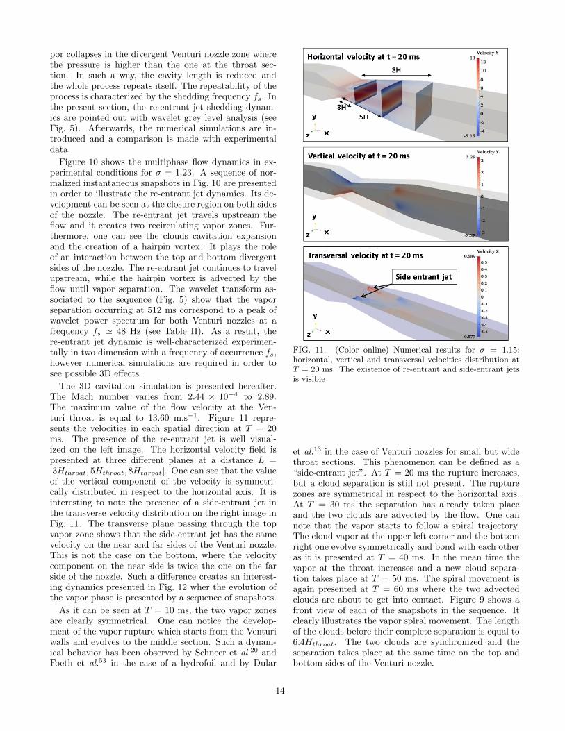
The 3D cavitation simulation is presented hereafter.The Mach number varies from 2.44 × 10⁻⁴ to 2.89.The maximum value of the flow velocity at the Ven-turi throat is equal to 13.60 m.s−1. Figure 11 repre-sents the velocities in each spatial direction at T = 20ms. The presence of the re-entrant jet is well visual-ized on the left image. The horizontal velocity field ispresented at three different planes at a distance L =[3Hthroat, 5Hthroat, 8Hthroat]. One can see that the valueof the vertical component of the velocity is symmetri-cally distributed in respect to the horizontal axis. It isinteresting to note the presence of a side-entrant jet inthe transverse velocity distribution on the right image inFig. 11. The transverse plane passing through the topvapor zone shows that the side-entrant jet has the samevelocity on the near and far sides of the Venturi nozzle.This is not the case on the bottom, where the velocitycomponent on the near side is twice the one on the farside of the nozzle. Such a difference creates an interest-ing dynamics presented in Fig. 12 wher the evolution ofthe vapor phase is presented by a sequence of snapshots.
As it can be seen at T = 10 ms, the two vapor zonesare clearly symmetrical. One can notice the develop-ment of the vapor rupture which starts from the Venturiwalls and evolves to the middle section. Such a dynam-ical behavior has been observed by Schneer et al.20 andFoeth et al.53 in the case of a hydrofoil and by Dular
FIG. 11. (Color online) Numerical results for σ = 1.15:horizontal, vertical and transversal velocities distribution atT = 20 ms. The existence of re-entrant and side-entrant jetsis visible
et al.13 in the case of Venturi nozzles for small but widethroat sections. This phenomenon can be defined as a“side-entrant jet”. At T = 20 ms the rupture increases,but a cloud separation is still not present. The rupturezones are symmetrical in respect to the horizontal axis.At T = 30 ms the separation has already taken placeand the two clouds are advected by the flow. One cannote that the vapor starts to follow a spiral trajectory.The cloud vapor at the upper left corner and the bottomright one evolve symmetrically and bond with each otheras it is presented at T = 40 ms. In the mean time thevapor at the throat increases and a new cloud separa-tion takes place at T = 50 ms. The spiral movement isagain presented at T = 60 ms where the two advectedclouds are about to get into contact. Figure 9 shows afront view of each of the snapshots in the sequence. Itclearly illustrates the vapor spiral movement. The lengthof the clouds before their complete separation is equal to6.4Hthroat. The two clouds are synchronized and theseparation takes place at the same time on the top andbottom sides of the Venturi nozzle.
14
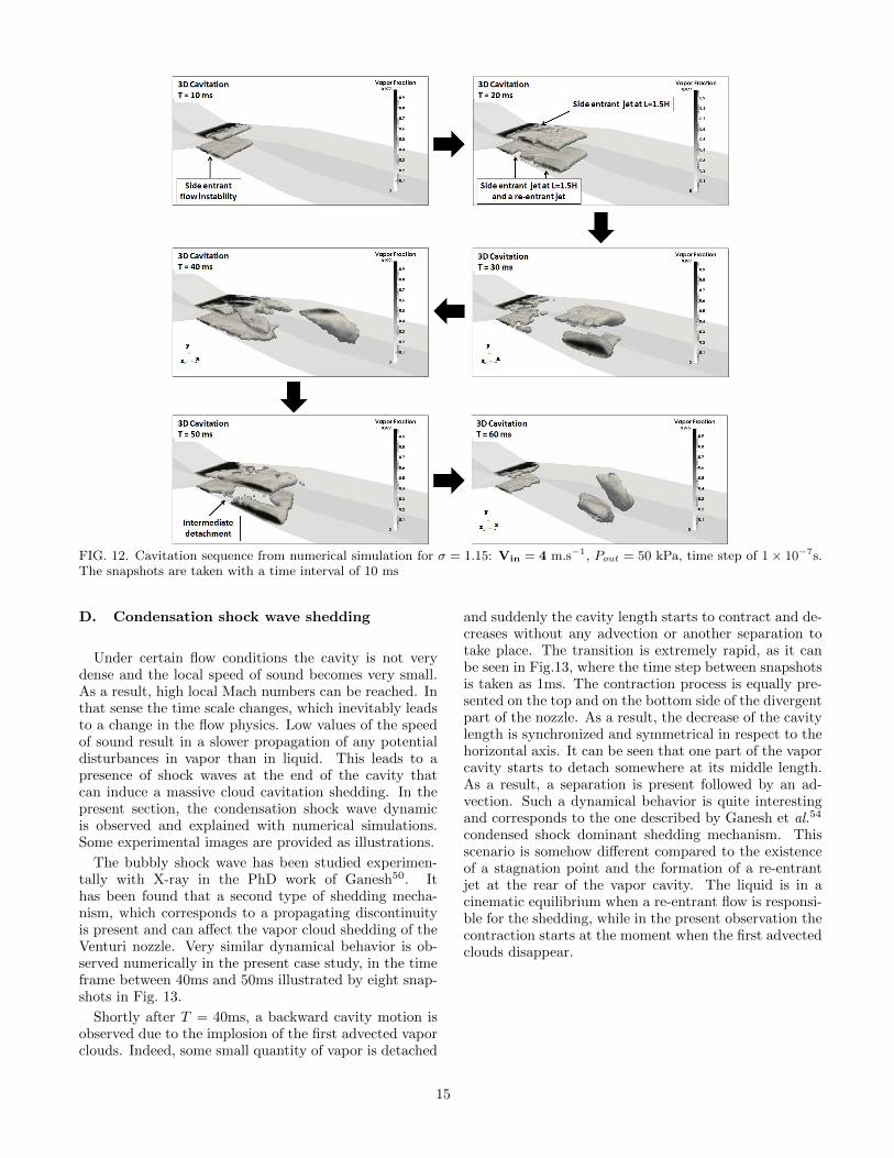
FIG. 12. Cavitation sequence from numerical simulation for σ = 1.15: Vin = 4 m.s−1, Pout = 50 kPa, time step of 1× 10⁻⁷s.The snapshots are taken with a time interval of 10 ms
D. Condensation shock wave shedding
Under certain flow conditions the cavity is not verydense and the local speed of sound becomes very small.As a result, high local Mach numbers can be reached. Inthat sense the time scale changes, which inevitably leadsto a change in the flow physics. Low values of the speedof sound result in a slower propagation of any potentialdisturbances in vapor than in liquid. This leads to apresence of shock waves at the end of the cavity thatcan induce a massive cloud cavitation shedding. In thepresent section, the condensation shock wave dynamicis observed and explained with numerical simulations.Some experimental images are provided as illustrations.
The bubbly shock wave has been studied experimen-tally with X-ray in the PhD work of Ganesh50. Ithas been found that a second type of shedding mecha-nism, which corresponds to a propagating discontinuityis present and can affect the vapor cloud shedding of theVenturi nozzle. Very similar dynamical behavior is ob-served numerically in the present case study, in the timeframe between 40ms and 50ms illustrated by eight snap-shots in Fig. 13.
Shortly after T = 40ms, a backward cavity motion isobserved due to the implosion of the first advected vaporclouds. Indeed, some small quantity of vapor is detached
and suddenly the cavity length starts to contract and de-creases without any advection or another separation totake place. The transition is extremely rapid, as it canbe seen in Fig.13, where the time step between snapshotsis taken as 1ms. The contraction process is equally pre-sented on the top and on the bottom side of the divergentpart of the nozzle. As a result, the decrease of the cavitylength is synchronized and symmetrical in respect to thehorizontal axis. It can be seen that one part of the vaporcavity starts to detach somewhere at its middle length.As a result, a separation is present followed by an ad-vection. Such a dynamical behavior is quite interestingand corresponds to the one described by Ganesh et al.54
condensed shock dominant shedding mechanism. Thisscenario is somehow different compared to the existenceof a stagnation point and the formation of a re-entrantjet at the rear of the vapor cavity. The liquid is in acinematic equilibrium when a re-entrant flow is responsi-ble for the shedding, while in the present observation thecontraction starts at the moment when the first advectedclouds disappear.
15
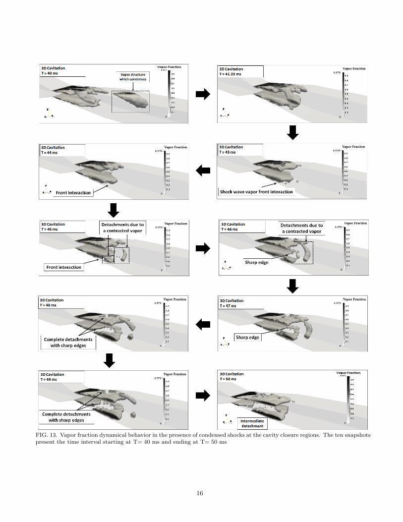
FIG. 13. Vapor fraction dynamical behavior in the presence of condensed shocks at the cavity closure regions. The ten snapshotspresent the time interval starting at T= 40 ms and ending at T= 50 ms
16
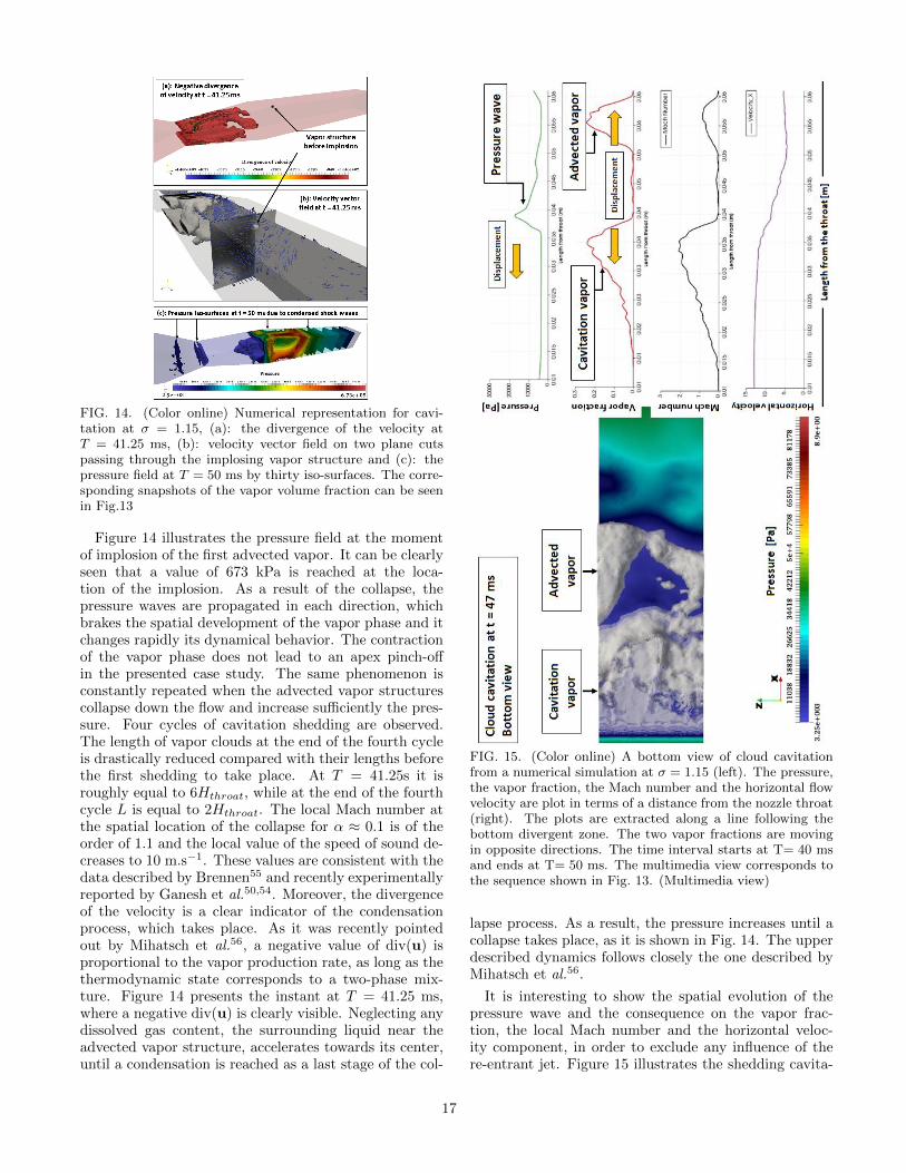
FIG. 14. (Color online) Numerical representation for cavi-tation at σ = 1.15, (a): the divergence of the velocity atT = 41.25 ms, (b): velocity vector field on two plane cutspassing through the implosing vapor structure and (c): thepressure field at T = 50 ms by thirty iso-surfaces. The corre-sponding snapshots of the vapor volume fraction can be seenin Fig.13
Figure 14 illustrates the pressure field at the momentof implosion of the first advected vapor. It can be clearlyseen that a value of 673 kPa is reached at the loca-tion of the implosion. As a result of the collapse, thepressure waves are propagated in each direction, whichbrakes the spatial development of the vapor phase and itchanges rapidly its dynamical behavior. The contractionof the vapor phase does not lead to an apex pinch-offin the presented case study. The same phenomenon isconstantly repeated when the advected vapor structurescollapse down the flow and increase sufficiently the pres-sure. Four cycles of cavitation shedding are observed.The length of vapor clouds at the end of the fourth cycleis drastically reduced compared with their lengths beforethe first shedding to take place. At T = 41.25s it isroughly equal to 6Hthroat, while at the end of the fourthcycle L is equal to 2Hthroat. The local Mach number atthe spatial location of the collapse for α ≈ 0.1 is of theorder of 1.1 and the local value of the speed of sound de-creases to 10 m.s−1. These values are consistent with thedata described by Brennen55 and recently experimentallyreported by Ganesh et al.50,54. Moreover, the divergenceof the velocity is a clear indicator of the condensationprocess, which takes place. As it was recently pointedout by Mihatsch et al.56, a negative value of div(u) isproportional to the vapor production rate, as long as thethermodynamic state corresponds to a two-phase mix-ture. Figure 14 presents the instant at T = 41.25 ms,where a negative div(u) is clearly visible. Neglecting anydissolved gas content, the surrounding liquid near theadvected vapor structure, accelerates towards its center,until a condensation is reached as a last stage of the col-
FIG. 15. (Color online) A bottom view of cloud cavitationfrom a numerical simulation at σ = 1.15 (left). The pressure,the vapor fraction, the Mach number and the horizontal flowvelocity are plot in terms of a distance from the nozzle throat(right). The plots are extracted along a line following thebottom divergent zone. The two vapor fractions are movingin opposite directions. The time interval starts at T= 40 msand ends at T= 50 ms. The multimedia view corresponds tothe sequence shown in Fig. 13. (Multimedia view)
lapse process. As a result, the pressure increases until acollapse takes place, as it is shown in Fig. 14. The upperdescribed dynamics follows closely the one described byMihatsch et al.56.
It is interesting to show the spatial evolution of thepressure wave and the consequence on the vapor frac-tion, the local Mach number and the horizontal veloc-ity component, in order to exclude any influence of there-entrant jet. Figure 15 illustrates the shedding cavita-
17
tion seen from the bottom, as well as the correspondingevolution of the pressure wave. It can be seen that thewave moves in an opposite the flow direction. At a cer-tain moment, the vapor fraction is cut by the wave intotwo smaller structures. Each one of them moves intoopposite directions. The Mach number reaches local val-ues of of the order of 3. The horizontal component ofthe flow velocity stays constantly positive which impliesthat no re-entrant jet effects are present. For more de-tails the reader is kindly advised to see the supplemen-tary material at Fig. 15. A value of 5.02 m.s−1 for theshock wave velocity propagation is estimated (for a timeperiod of 3.5 × 10⁻³s the shock wave moves forward at1.76 × 10−2m). The obtained velocity has the same or-der of magnitude and fits in the range of values given byGanesh50.
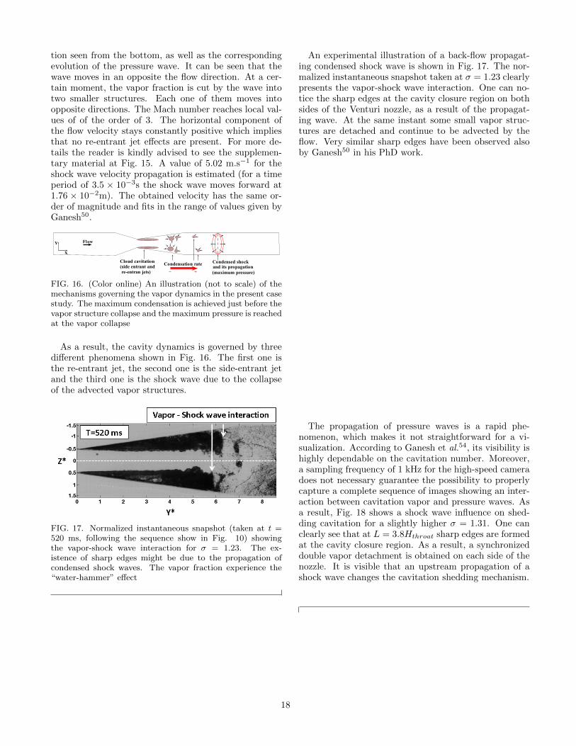
FIG. 16. (Color online) An illustration (not to scale) of themechanisms governing the vapor dynamics in the present casestudy. The maximum condensation is achieved just before thevapor structure collapse and the maximum pressure is reachedat the vapor collapse
As a result, the cavity dynamics is governed by threedifferent phenomena shown in Fig. 16. The first one isthe re-entrant jet, the second one is the side-entrant jetand the third one is the shock wave due to the collapseof the advected vapor structures.
FIG. 17. Normalized instantaneous snapshot (taken at t =520 ms, following the sequence show in Fig. 10) showingthe vapor-shock wave interaction for σ = 1.23. The ex-istence of sharp edges might be due to the propagation ofcondensed shock waves. The vapor fraction experience the“water-hammer” effect
An experimental illustration of a back-flow propagat-ing condensed shock wave is shown in Fig. 17. The nor-malized instantaneous snapshot taken at σ = 1.23 clearlypresents the vapor-shock wave interaction. One can no-tice the sharp edges at the cavity closure region on bothsides of the Venturi nozzle, as a result of the propagat-ing wave. At the same instant some small vapor struc-tures are detached and continue to be advected by theflow. Very similar sharp edges have been observed alsoby Ganesh50 in his PhD work.
The propagation of pressure waves is a rapid phe-nomenon, which makes it not straightforward for a vi-sualization. According to Ganesh et al.54, its visibility ishighly dependable on the cavitation number. Moreover,a sampling frequency of 1 kHz for the high-speed cameradoes not necessary guarantee the possibility to properlycapture a complete sequence of images showing an inter-action between cavitation vapor and pressure waves. Asa result, Fig. 18 shows a shock wave influence on shed-ding cavitation for a slightly higher σ = 1.31. One canclearly see that at L = 3.8Hthroat sharp edges are formedat the cavity closure region. As a result, a synchronizeddouble vapor detachment is obtained on each side of thenozzle. It is visible that an upstream propagation of ashock wave changes the cavitation shedding mechanism.
18
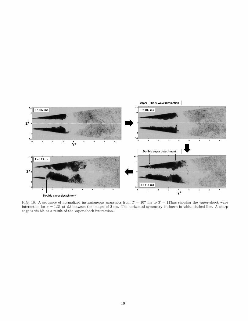
FIG. 18. A sequence of normalized instantaneous snapshots from T = 107 ms to T = 113ms showing the vapor-shock waveinteraction for σ = 1.31 at ∆t between the images of 2 ms. The horizontal symmetry is shown in white dashed line. A sharpedge is visible as a result of the vapor-shock interaction.
19
IV. CONCLUSIONS
In the present paper, “transitory” cavitation regimehas been investigated numerically in 3D and experimen-tally in 2D. For a constant inlet flow, a small range ofcavitation numbers, where two cloud cavitation sheddingmechanisms coexist, has been studied experimentally. Aclassical evolution of cavity closure position as a func-tion of cavitation number has been observed and twofrequencies of cloud shedding, increasing with the cav-itation number, have been highlighted. The choice hasbeen made to focus only on one case with a correspond-ing cavitation number σ = 1.23 in order to study thedynamics of the two-phase system.
The use of a “full” 3D compressible code is justifiedby the fact that the re-entrant jet flow is not the onlyobserved closure mechanism. Indeed, for σ = 1.15 a side-entrant jet, hardly observable experimentally, is found tobe responsible for the partial cut of the void fraction. Itsdevelopment was found to be symmetrical. A key find-ing, which was firstly detected in a 3D simulation, is theinfluence of the shock waves due to collapses of the vaporstructures. They play the role of sudden “break” for thespatial development of the vapor clouds. As a result, thecavity dynamics is governed by three different phenom-ena, which are the re-entrant jet, the side-entrant jet andthe condensation shock waves. Consequently the symme-try between the two side cavities can be broken due toa scale effect resulting in a side-entrant jet. All of thesephenomena have been experimentally observed on imagesequences, and have been identified with a wavelet tech-nique. Their frequencies of occurrence as well as theirtemporal positions are revealed.
The snapshot Proper Orthogonal Decomposition tech-nique has been used on numerical and experimental dataas a complementary tool for the study of the cavitation“transitory” regime at σ = 1.15. The three different sec-tion cuts show very similar results in terms of energycontributions, but differ in their spatial modal distribu-tion.The number of cycles in experimental case is higherthan in simulations, which leads to more significant re-sults. The decomposition into 10 modes and the presen-tation of the first four is found to be sufficient for thegood representation of the flow behavior. The values ofthe energy contribution for all of the modes 1 are supe-rior to 1%, which implies the presence of cloud cavitationregime. The POD analysis reveals a clear horizontal sym-metry of the multiphase flow for the experimental caseand the superposed numerical one.
ACKNOWLEDGEMENT
The authors would like to acknowledge the financialsupport for the PhD thesis granted by SNECMA, part ofSAFRAN group.
Appendix A: Development speed of sound inliquid
The constant entropy is given in Eq.A1 which afterrewriting in terms of pressure and
c2 =
(∂p
∂ρ
)s
(A1)
temperature using Maxwell’s relations, gives:
c2 =ρ(∂h∂T
)p(
∂ρ∂p
)T
(∂h∂T
)p
+(∂ρ∂T
)p
[1− ρ
(∂h∂p
)T
] (A2)
Moreover, the use of Maxwell’s relation Eq.A2 enables usto write down:
∂cv(T, v)
∂v= T
∂2p
∂T 2(A3)
One can also write the internal energy in terms of thepressure and volume at constants volume and tempera-ture, respectively as follows:(
∂e
∂T
)v
= cv(v, T ) (A4)
(∂e
∂v
)T
= −t+ T
(∂p
∂T
)v
(A5)
If we use the hypothesis that the density of the liquidis constant, i.e. the liquid is incompressible, as well ascv (ρ0, T ) to be constant, one can write the formulationfor the speed of sound in the liquid phase:
c2l =N(p− psat(T ) +K0)
ρ+
p
ρ2Cvl
(∂psat(T )
∂T− N(p− psat(T ) +K0)
ρl,sat(T )
∂ρsat(T )
∂T
)(A6)
Appendix B: Phase transition algorithm
20
Algorithm 1: Phase transition algorithmData: ρn, (ρu)n, (ρv)n, (ρw)n, (ρE)n, T n : computed at previous time stepResult: ρn+1, (ρu)n+1, (ρv)n+1, (ρw)n+1, (ρE)n+1 : given by solving Navier-Stokes equationsCompute: en+1 = En+1 − 1
2 ((un+1)2 + (vn+1)2 + (wn+1)2);
Initialize: T n+1 = T n;repeat
(Re)-initialize: T ∗ = T n+1;Compute: ρl,sat(T ∗) and ρv,sat(T ∗);if ρn+1 > ρl,sat(T ∗) then
α = 0; /* liquid */T n+1 = en+1 − el0Cvl + T0
endif ρn+1 < ρv,sat(T ∗) then
α = 1; /* vapor */T n+1 = en+1 − el0 −Lv(T0)Cvv + T0
endif ρv,sat(T ∗) ≤ ρn+1 ≤ ρl,sat(T ∗) then
α = ρn+1 − ρl,sat(T ∗)ρv,sat(T ∗)− ρl,sat(T ∗); /* mixture */Solve: T n+1 =ρn+1en+1 −αρv,sat(T n+1)Lv(T0)− ρn+1el0αρv,sat(T n+1)Cvv + (1−α)ρl,sat(T n+1)Cvl + T0
enduntil |T n+1 − T ∗| ≤ ε;/* Computation of other parameters */;if α = 0 then
pn+1 = K0
[(ρn+1ρl,sat(T n+1)
)N − 1]+ Psat(T n+1);
µn+1 = µref 10Tref T
n+1−S0;(cn+1)2 =NP ρn+1 + pn+1(ρn+1)2Cvl
(Psat(T n+1)T −NP ρl,sat(T n+1)ρl,sat(T n+1)T
);
where P = pn+1 − Psat(T n+1) +K0;endif α = 1 then
pn+1 = (γ − 1)ρn+1en+1;µn+1 = µref T n+1 + S0Tref + S0
(T n+1Tref
)1.5;
λv = a1T + a2T 2 + a3T 3 + a4T 4;(cn+1)2 = γpn+1ρn+1;
endif 0 < α < 1 then
pn+1 = Psat(T n+1);1µn+1 =
1−ξµn+1l
+ ξµn+1v
;
λv = a1T + a2T 2 + a3T 3 + a4T 4;where,µn+1l = µl,ref 10
Tl,ref Tn+1−Sl,0 ;
µn+1v = µv,ref T n+1 + Sv,0Tv,ref + Sv,0(T n+1Tv,ref
)1.5;
(cn+1)2 = ρn+1(αρv,sat(cn+1v )2 +1−αρl,sat(cn+1l )2
)−1;
where,(cn+1l )2 =NP ρn+1 + pn+1(ρn+1)2Cvl
(Psat(T n+1)T −NP ρl,sat(T n+1)ρl,sat(T n+1)T
);
(cn+1v )2 = γpn+1ρn+1;end
Compute: Hn+1 = En+1 + pn+1
ρn+1
21
REFERENCES
1R. Fortes-Patella and J.-L. Reboud. A new approach toevaluate the cavitation erosion power. J. Fluids Eng.,120:335–344, 1998.
2Y. Tsujimoto, K. Kamijo, and C. E. Brennen. Unifiedtreatment of flow instabilities of turbomachines. Int.J. Prop. and Power, 17:636–643, 2001.
3B. Pouffary, R. Fortes-Patella, J.-L. Reboud, and P.-A.Lambert. Numerical simulation of 3d cavitating flows:Analysis of cavitation head drop in turbomachinery. J.Fluids Eng., 130:061301, 2008.
4I. Mejri, F. Bakir, R. Rey, and T. Belamri. Comparisonof computational results obtained from a homogeneouscavitation model with experimental investigations ofthree inducers. J. Fluids Eng., 128:1308–1323, 2006.
5A. Danlos, J. E. Mehal, F. Ravelet, O. Coutier-Delgosha, and F. Bakir. Study of the cavitating in-stability on a grooved venturi profile. Int. J. Heat andFluid Flow, 136:101302, 2014.
6P. Brandner, G. J. Walker, P. N. Niekamp, and B. An-derson. An experimental investigation of cloud cavi-tation about a sphere. J. Fluid Mech., 656:147–176,2010.
7M. Wosnik and R. E. A. Arndt. Measurements in highvoid-fraction bubbly wakes created by ventilated su-percavitation. J. Fluids Eng., 135:011304, 2013.
8S. L. Ceccio. Friction drag reduction of external flowswith bubble and gas injection. Ann. Rev. Fluid Mech.,42:183–203, 2010.
9Q. Le, J.P. Franc, and J.M. Michel. Partial cavities:Global behavior and mean pressure distribution. J.Fluids Eng., 115:243–248, 1993.
10T.M. Pham, F. Larrarte, and D.H. Fruman. Investiga-tion of unsteady sheet cavitation and cloud cavitationmechanisms. J. Fluids Eng., 121:289–296, 1999.
11M. Callenaere, J. P. Franc, J.M. Michel, and M. Rion-det. The cavitation instability induced by the develop-ment of a re-entrant jet. J. Fluid Mech., 444:223–256,2001.
12B. Stutz and J.-L. Reboud. Measurements within un-steady cavitation. Exp. In Fluids, 29:545–552, 2000.
13M. Dular, I. Khlifa, S. Fuzier, M. Adama Maiga, andO. Coutier-Delgosha. Scale effect on unsteady cloudcavitation. Exp. In Fluids, 53:1233–1250, 2012.
14H. Ganesh, S. A. Makiharju, and S. L. Ceccio. Partialcavity shedding due to the propagation of shock wavesin bubbly flows. Proceedings of the 30th symposium onnaval hydrodynamics, 2014.
15J. Decaix and E. Goncalves. Investigation of three-dimensional effects on a cavitating venturi flow. Int. J.Heat and Fluid Flow, 44:576–595, 2013.
16G. Chen, G. Wang, C. Hu, B. Huang, Y. Gao, andM. Zhang. Combined experimental and computationalinvestigation of cavitation evolution and excited pres-sure fluctuation in a convergent-divergent channel. Int.J. Multiphase Flow, 72:133–140, 2015.
17N. Dittakavi, A. Chunekar, and S. Frankel. Large eddysimulation of turbulent-cavitation interactions in a ven-turi nozzle. J. Fluids Eng., 132:121301, 2010.
18B. Charriere, J. Decaix, and E. Goncalves. A compar-ative study of cavitation models in a venturi flow. Eur.J. Mech. B/Fluids, 49:287–297, 2015.
19P. Tomov, S. Khelladi, F. Ravelet, C. Sarraf, F. Bakir,and P. Vertenoeuil. Experimental study of aerated cavi-tation in a horizontal venturi nozzle. Exp. Thermal andFluid Science, 70:85–95, 2016.
20G. H. Schnerr, I. H. Sezal, and S. J. Schmidt. Numeri-cal investigation of three-dimensional cloud cavitationwith special emphasis on collapse induced shock dy-namics. Phys. Fluids, 20, 2008.
21M. Dular and R. Bachert. The issue of strouhal numberdefinition in cavitating flow. J. of Mech. Eng., 55:666–674, 2009.
22R. Saurel, J. P. Cocchi, and P. B. Butler. Numericalstudy of cavitation in the wake of a hypervelocity un-derwater projectile. Int. J. Prop. and Power, 15:513–522, 1999.
23O. Le Metayer, J. Massoni, and R. Saurel. Elaborationdes lois d’etat d’un liquide et de sa vapeur pour lesmodeles d’ecoulements diphasiques. Int. J. ThermalScience., 43:265–276, 2004.
24E. Schmidt. Properties of Water and Steam in SI-Units; 0-800◦C, 0-1000 bar. Springer-Verlag, 1989.
25H. Vogel. Phys. Z., 22:645, 1921.26G.S. Fulcher. J. Am. Ceram. Soc., 8:339, 1925.27G.S. Fulcher and W. Hesse. Z. Anorg. Allg. Chem.,
156:245, 1926.28W. Sutherland. The viscosity of gases and molecu-
lar force. Philosophical Magazine Series 5, 36:507–531,1893.
29I. Dincer, C.O. Colpan, O. Kizilkan, and M.A. Ezan.Progress in Clean Energy, Volume 2. Novel Systemsand Applications. Springer-Verlag, 2015.
30A. Wood. A text book of sound. G. Bell and Sons Ltd.London, 1960.
31R. Saurel, P. Boivin, and O. Le Metayer. A general for-mulation for cavitating , boiling and evaporating flows.Computers & Fluids, 128:53–64, 2016.
32S. Khelladi, X. Nogueira, F. Bakir, and I. Colominas.Toward a higher order unsteady finite volume solverbased on reproducing kernel methods. Comp. Meth. inApp. Mech. and Eng., 200:2348–2362, 2011.
33X. Nogueira, I. Colominas, L. Cueto-Felgueroso, andS. Khelladi. On the simulation of wave propagationwith a higher-order finite volume scheme based on re-producing kernel methods. Comp. Meth. in App. Mech.and Eng., 199:1471–1490, 2010.
34X. Nogueira, S. Khelladi, L. Cueto-Felgueroso,F. Bakir, I. Colominas, and H. Gomez. Implicit large-eddy simulation with a moving least squares-based fi-nite volume method. IOP Conference Series: MaterialsScience and Engineering, 10:012235, 2010.
35E. Turkel. Review of preconditioning methods for fluiddynamics. Applied Numerical Mathematics, 12:257–
22
284, 1993.36X. Nogueira, L. Ramirez, S. Khelladi, J.-C. Chassaing,
and I. Colominas. A high-order density-based finitevolume method for the computation of all-speed flows.Comp. Meth. in App. Mech. and Eng., 298:229–251,2016.
37E. Shima and K. Kitamura. On new simple low-dissipation scheme of ausm-family for all speeds. AIAApaper, 49:1–15, 2009.
38K. Kitamura, M.-S. Liou, and C.-h. Chang. Exten-sion and comparative study of ausm-family schemes forcompressible multiphase flow simulations. Commun.Comput. Phys., 1:632–674, 2006.
39S. Hickel. Implicit Turbulence Modeling for Large-Eddy Simulation. PhD thesis, Technische UniversitatMunchen, 2008.
40X. Nogueira, L. Cueto-Felgueroso, I. Colominas, andH. Gomez. Implicit large eddy simulation of non-wall-bounded turbulent flows based on the multiscale prop-erties of a high-order finite volume method. Comp.Meth. in App. Mech. and Eng., 199:615–624, 2010.
41P. Holmes, G. Berkooz, and J. Lumley. Turbulence, Co-herent Structures, Dynamical Systems and Symmetry.Cambridge University Press, 2013.
42A. Danlos, F. Ravelet, O. Coutier-Delgosha, andF. Bakir. Cavitation regime detection through properorthogonal decomposition: Dynamics analysis of thesheet cavity on a grooved convergentdivergent nozzle.Int. J. Heat and Fluid Flow, 47:9–20, 2014.
43B. Patte-Rouland, A. Danlos, G. Lalizel, E. Rouland,and P. Paranthoen. Proper orthogonal decompositionused for determination of the convection velocity of theinitial zone of the annular jet. aerodynamic study andcontrol of instabilities. J. of Fluid Dynamics, 1:1–10,2012.
44E. A. Christensen, M. Brons, and J. N. Sorensen. Eval-uation of pod-based decomposition techniques appliedto parameter-dependent non-turbulent flows. SIAMJournal of Scientific Computing, 21:1419–1434, 2000.
45T. Brenner. Practical aspects of the implementation ofreduced-order models based on proper orthogonal de-
composition. PhD Thesis, University of Texas Austin,2011.
46L. Sirovich. Turbulence and the dynamics of coherentstructures part one: coherent structures. Quarterly ofApplied Mathematics, XLV:561–571, 1987.
47M. Kjeldsen and R. E. A. Arndt. Joint time frequencyanalysis techniques : a study of transitional dynamicsin sheet/cloud cavitation. In Symposium on Cavitation,2001.
48P. Brandner, B. W. Pierce, and K. L. de Graaf. Cavita-tion about a jet in crossflow. J. Fluid Mech., 768:141–174, 2015.
49C. Torrence and G. P. Compo. A practical guide towavelet analysis. Bull. Amer. Meteor. Soc, 79, 1999.
50H. Ganesh. Bubbly shock propagation as a cause ofsheet to cloud transition of partial cavitation and sta-tionary cavitation bubbles forming on a delta wing vor-tex. PhD thesis, University of Michigan, 2015.
51P. Tomov, A. Danlos, S. Khelladi, F. Ravelet, SarrafC., and F. Bakir. Pod study of aerated cavitation in aventuri nozzle. Journal of Physics: Conference Series,656:012171, 2015.
52R. B. Wade and A. J. Acosta. Experimental Observa-tions on the Flow Past a Plano-Convex Hydrofoil. J.Basic Eng., 88:273–282, 1966.
53E.-J. Foeth, T. van Terwisga, and C. van Doorne. Onthe collapse structure of an attached cavity on a three-dimensional hydrofoil. J. Fluids Eng., 130:071303,2008.
54H. Ganesh, S. A. Makiharju, and S. L. Ceccio. Inter-action of a compressible bubbly flow with an obsta-cle placed within a shedding partial cavity. Journal ofPhysics: Conference Series, 656:012151, 2015.
55C. E. Brennen. Fundamentals of multiphase flow. Cam-bridge University Press, 2005.
56M. S. Mihatsch, S. J. Schmidt, and N. A. Adams.Cavitation erosion prediction based on analysis of flowdynamics and impact load spectra. Phys. Fluids,27:103302, 2015.
23