UNLV Retrospective Theses & Dissertations

1-1-1994

An application of Solow's growth model: Case of sub-Saharan An application of Solow's growth model: Case of sub-Saharan

Africa Africa

Maureen Sarahjane Miller University of Nevada, Las Vegas

Follow this and additional works at: https://digitalscholarship.unlv.edu/rtds

Repository Citation Repository Citation Miller, Maureen Sarahjane, "An application of Solow's growth model: Case of sub-Saharan Africa" (1994). UNLV Retrospective Theses & Dissertations. 419. http://dx.doi.org/10.25669/vggc-m70t

This Thesis is protected by copyright and/or related rights. It has been brought to you by Digital Scholarship@UNLV with permission from the rights-holder(s). You are free to use this Thesis in any way that is permitted by the copyright and related rights legislation that applies to your use. For other uses you need to obtain permission from the rights-holder(s) directly, unless additional rights are indicated by a Creative Commons license in the record and/or on the work itself. This Thesis has been accepted for inclusion in UNLV Retrospective Theses & Dissertations by an authorized administrator of Digital Scholarship@UNLV. For more information, please contact digitalscholarship@unlv.edu.

INFORMATION TO USERS

This manuscript has been reproduced from the microfilm master. UMI films the text directly from the original or copy submitted. Thus, some thesis and dissertation copies are in typewriter face, while others may be from any type of computer printer.

The quality of this reproduction is dependent upon the quality of the copy submitted. Broken or indistinct print, colored or poor quality illustrations and photographs, print bleedthrough, substandard margins, and improper alignment can adversely afreet reproduction.

In the unlikely event that the author did not send UMI a complete manuscript and there are missing pages, these will be noted. Also, if unauthorized copyright material had to be removed, a note will indicate the deletion.

Oversize materials (e.g., maps, drawings, charts) are reproduced by sectioning the original, beginning at the upper left-hand comer and continuing from left to right in equal sections with small overlaps. Each original is also photographed in one exposure and is included in reduced form at the back of the book.

Photographs included in the original manuscript have been reproduced xerographically in this copy. Higher quality 6" x 9" black and white photographic prints are available for any photographs or illustrations appearing in this copy for an additional charge. Contact UMI directly to order.

A Bell & Howell Information Company 300 North Z eeb Road. Ann Arbor. Ml 48106-1346 USA

313/761-4700 800/521-0600

AN APPLICATION OF SOLOW’S GROWTH MODEL: CASE OF

SUB-SAHARAN AFRICA

by

Maureen Miller

A thesis submitted in partial fulfillment of the requirements for the degree of

Master of Arts

in

Economics

Department of Economics University of Nevada, Las Vegas

December 1994

OMI Number: 1361095

Copyright 1995 by Miller, Maureen Sarahjane

All rights reserved.

UMI Microform Edition 1361095 Copyright 1995, by UMI Company. All rights reserved.

This microform edition is protected against unauthorized copying under Title 17, United States Code.

UMI300 North Zeeb Road Ann Arbor, MI 48103

® 1995 Maureen Miller All Rights Reserved

APPROVAL

The thesis of Maureen Miller for the Degree of Master of Arts in Economics is approved.

J __\\ S lA o . \ j ? *

Chairperson, Djeto Assane, Ph.D.

Examining Committee Member, Nasser Daneshvary, Ph.D.

Examining Committee Member, Lein-Lein Chen, Ph.D.

s ---

Graduate Faculty Representative, Hailu Abatena, Ph.D.

Graduate Dean, Ronald W. Smith, Ph.D.

University of Nevada Las Vegas, Nevada

December 1994

1 1

ABSTRACT

This study is prompted by the growing concern over the poor economic

performance of Sub-Saharan Africa (SSA) relative to the rest of the world over the

past decade. The purpose of the study is to examine how a simple and predictable

model like Solow’s model can explain per capita income in SSA. Our study consists

of cross-sectional-cum-time-series regressions using 32 SSA countries. The time span

considered is a 26-year period from 1960 to 1985. The model is based on the

empirical framework developed by Mankiw et al. (1992). Our results show that saving

has a significantly positive impact on per capita GDP in SSA, while population

growth rate, though consistently negative, is significant only at higher levels of data

disaggregation. Our findings are consistent with Mankiw et al.’s (1992) which confirm

Solow’s predictions that saving has a positive effect on per capita income whereas

population growth has a negative effect.

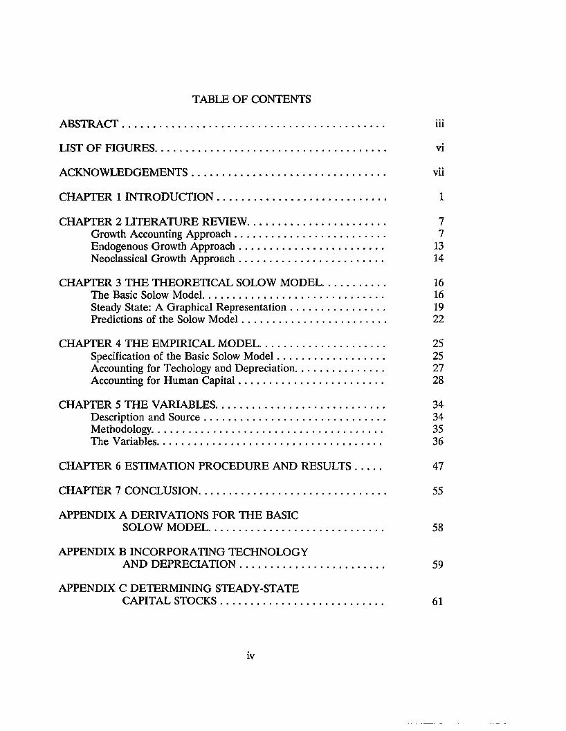
TABLE OF CONTENTS

ABSTRACT.............................................................................................. iii

LIST OF FIGURES................................................................................... vi

ACKNOWLEDGEMENTS...................................................................... vii

CHAPTER 1 INTRODUCTION............................................................. 1

CHAPTER 2 LITERATURE REVIEW.................................................. 7Growth Accounting Approach...................................................... 7Endogenous Growth Approach.................................................... 13Neoclassical Growth Approach.................................................... 14

CHAPTER 3 THE THEORETICAL SOLOW MODEL....................... 16The Basic Solow Model................................................................. 16Steady State: A Graphical Representation.................................. 19Predictions of the Solow M odel.................................................... 22

CHAPTER 4 THE EMPIRICAL MODEL............................................. 25Specification of the Basic Solow M odel...................................... 25Accounting for Techology and Depreciation................................ 27Accounting for Human Capital.................................................... 28

CHAPTER 5 THE VARIABLES............................................................. 34Description and Source................................................................. 34Methodology................................................................................... 35The Variables................................................................................. 36

CHAPTER 6 ESTIMATION PROCEDURE AND RESULTS 47

CHAPTER 7 CONCLUSION................................................................... 55

APPENDIX A DERIVATIONS FOR THE BASICSOLOW MODEL............................................................... 58

APPENDIX B INCORPORATING TECHNOLOGYAND DEPRECIATION.................................................... 59

APPENDIX C DETERMINING STEADY-STATECAPITAL STOCKS........................................................... 61

iv

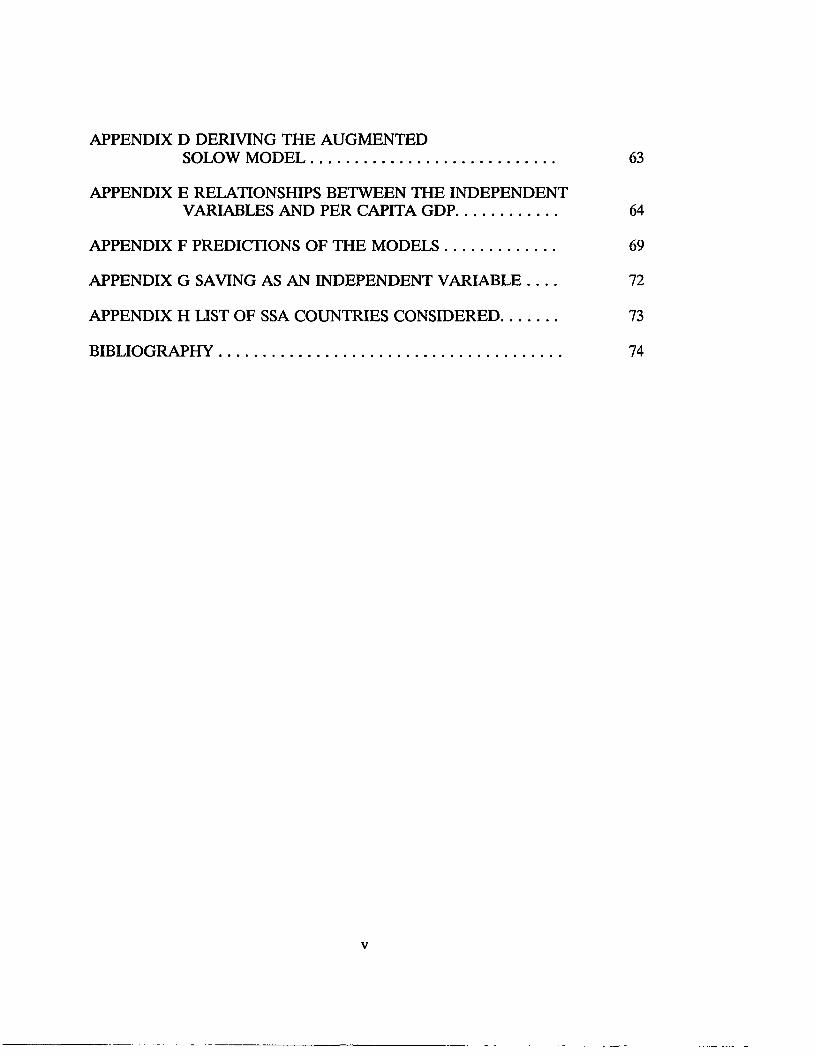
APPENDIX D DERIVING THE AUGMENTEDSOLOW MODEL............................................................. 63

APPENDIX E RELATIONSHIPS BETWEEN THE INDEPENDENTVARIABLES AND PER CAPITA GDP......................... 64

APPENDIX F PREDICTIONS OF THE MODELS........................... 69

APPENDIX G SAVING AS AN INDEPENDENT VARIABLE 72

APPENDIX H LIST OF SSA COUNTRIES CONSIDERED.............. 73

BIBLIOGRAPHY..................................................................................... 74

v

LIST OF FIGURES

Figure 1 Steady State-A Graphical Representation............................... 21Figure 2 Changes in the Saving Rate........................................................ 24Figure 3 Changes in the Population Growth R a te ................................. 24Figure 4a Per Capita GDP and Saving- 1960-85 .................................... 40Figure 4b Per Capita GDP and Investment-1960-85................................ 40Figure 5 Per Capita GDP and Population Growth-1960-85 .................. 43Figure 6 Per Capita GDP and Schooling-1960-85 .................................. 46

ACKNOWLEDGEMENTS

I would like to express my most profound appreciation to the Chair of my

Thesis Committee, Dr. Djeto Assane. His immense caring and patient guidance have

allowed me to grow in understanding.

My earnest thanks go to the members of my committee, Dr. Lein-Lein Chen,

Dr. Nasser Daneshvary, and Dr. Hailu Abatena. Dr. Chen’s enthusiasm and sincere

interest in my work have been very inspiring. I am deeply grateful to Dr. Daneshvary

for his support throughout my graduate program. Dr. Abatena has been very

encouraging and made useful comments.

I am indebted to my fellow graduate students and to the team of the Center

for Business and Economic Research for their help and reassurance. I am specially

thankful to the department secretary, Judy Feliz, and to Barbara DiPaolo in the

Dean’s Office, for patiently listening and cheering me on during times of

discouragement.

I would like to acknowledge the invaluable support provided by my husband

during this very eventful program.

CHAPTER 1

INTRODUCTION

There is growing concern over the worldwide decline in the rate of economic

growth. Aside from the Pacific Rim area, most regions of the world have experienced

lower per capita GDP growth rates in the 1970s and 1980s relative to the 1960s.1

The effects of the economic slowdown on living standards has generated renewed

interest in economic growth. It is widely believed that an understanding of the factors

influencing economic growth is necessary to formulate appropriate policies to reverse

the observed trend.

Although the oil price shock of the 1970s is cited as a turning point in this

economic slowdown, this event alone cannot explain the low growth rates that

persisted well into the 1980s. In particular, since the oil shock had worldwide

repercussions, how do we explain that non-oil exporting countries in the Pacific

enjoyed unabated growth for nearly three decades? Similarly, how do we explain

that countries with similar initial conditions have experienced divergent economic

growth performances in a span of three decades? For example, in the 1960s South

^ o r ld Bank, World Development Report. 1989; table A.2 p 146.

2

Korea and the Philippines had similar per capita incomes of about $640.2 They also

had fairly similar demographic and economic features. However, per capita income

of South Korea is now three times that of the Philippines. From the 1960s to the

1980s, per capita income in the two countries grew on average at 6.2% and 1.8%,

respectively.

Likewise, when Ghana and Malaysia became independent from Great Britain

in 1957, they both had "a rich mix of resources," and reserves of foreign currencies.3

Above all, they both had a per capita income of $750. Three and a half decades

later, per capita income in Malaysia was $2500, nearly six times that of Ghana.

This relatively slow growth in Ghana’s per capita income raises concerns about

the potential for economic development in Sub-Saharan Africa (SSA), where many

countries have experienced per capita GDP growth rates inferior to Ghana’s in the

1980s.4 The aggregate growth rate for SSA in the 1980s was -2.6% which stands in

sharp contrast with the post-independence performance, when on average SSA

countries grew at 2.0% and when investment returned an attractive rate of 30.7%

annually.

Recent studies have attempted to shed light on the drastically different growth

experiences as discussed above. They have characterized the East Asian performance

2Amount in U.S. dollars is in constant 1975 prices. Data for this paragraph are from R. E. Lucas, "Making a Miracle" Econometrica. March 1993.

3The Wall Street Journal, January 26, 1994.

4See World Bank, Sub-Saharan Africa-From Crisis to Sustainable Growth.1989.

as "productivity miracles" that allowed the typical worker to produce 6 times more

now than what he could produce in the 1960s.5 According to Lucas (1993) the

"miracle economies" have tended to engage in large scale exports of highly

sophisticated manufactures.6 Also, these economies were characterized by a higher

degree of urbanization, an increasingly well-educated population, a high savings rate,

and a pro-business government. Lucas (1993) argues that those features are indeed

part of "any explanation of the growth miracles" but are "not themselves

explanations." As such, "one needs...a theory" that can provide a framework for

analyzing growth.

Three major growth theories have been formulated over the past 40 years: the

Harrod-Domar model, the Solow model, and, lately, the Endogenous Growth model.

The Harrod-Domar model explains growth of output in a Keynesian framework,

assuming employment of fixed proportions of inputs. It emphasizes the dual character

of investment as income creating and as capacity expanding. As such, strict equality

between the actual and warranted growth rates is necessary to avert continuous

instability and spiralling economic decline. In this model, the economy is balanced

on a "knife-edge" equilibrium path because saving and investment decisions are made

by different economic agents.

5Lucas (1993).

6Lucas refers to economies, such as South Korea, that have experienced outstanding economic performance in the last decades as "miracle economies."

Solow’s 1956 growth model discards the fixed proportions assumption and

shows that an economy does not necessarily balance on a "razor-edge" path of

equilibrium growth. In the Solow model, a country moves toward a steady state

equilibrium where capital, labor, and output grow at the same rate. This implies that,

in steady state, per capita output and capital-labor ratio do not change. In this model,

an economy that is not in equilibrium moves toward steady state through changing

capital-labor ratios that arise from (i) a constantly growing population and (ii)

changes in the capital stock due to changes in domestic saving. Hence, the saving rate

influences long-run standard of living7 but not growth rate of per capita income.

However, the model attributes differences in growth rates between two countries with

identical production technologies and saving rates to diverging initial per capita

incomes. The model predicts that the country with the lower initial per capita income

will grow faster than and catch up with the other. Eventually, the two countries

converge toward similar steady state levels.8

The endogenous growth theory discards the assumptions of diminishing returns

to capital accumulation and of exogenous technological progress. It emphasizes the

roles of capital accumulation, externalities, and individual choice effects on human

7It can be shown diagrammatically that, for a given production function, a higher saving rate results in a higher per capita income, though not necessarily in a higher per capita consumption. If the saving rate initially corresponds to the Golden Rule level of consumption, increasing the saving rate, ceteris paribus, leads to a decline in per capita consumption. In this respect, steady state is dynamically inefficient.

’’Trade causes convergence to happen more quickly. See, for example, Plosser (1992), page 62.

capital.9 Although insightful and interesting, the endogenous growth theory relies on

variables that are difficult to measure empirically.10

In this study, we follow Mankiw et al.’s (1992) specification of Solow’s model

to analyze living standards in Sub-Saharan Africa.11 The findings of Mankiw et al.

support Solow’s predictions that ”[t]he higher the rate of saving, the richer the

country [and that the] higher the rate of population growth, the poorer the

country."12 There are compelling reasons for analyzing the influences of saving and

population growth in SSA.

First, SSA countries have been lagging in economic performance relative to

the rest of the world. Yet, the cross-sectional growth studies to date have mostly

analyzed groups comprised of developed as well as developing countries.13

Therefore, a study based solely on SSA data can point to some of the economic

factors that are pertinent to economic growth in that region.

9The endogenous theory allows a greater scope for policy in the determination of economic growth. See, for example, Kahn (1992).

10Pack, Howard, "Endogenous Growth Theory: Intellectual Appeal and Empirical Shortcomings" Journal of Economic Perspectives. Fall 1993, vol. 8, no. 1, p. 55-72.

“Mankiw, N. G., D. Romer, D. N. Weil, "A Contribution to the Empirics of Economic Growth," Quarterly Journal of Economics. May 1992.

“Knight et al. (1993) also obtained results supporting Solow’s predictions regarding the impacts of saving and population growth on per capita income.

“See, for example, works by Otani and Villanueva (1990), Landau (1983), Kormendi and Meguire (1985), Singh (1985), or Ram (1987).

Second, SSA forms a less heterogeneous group of countries than Less

Developed Countries (LDCs) as a whole, such that it is meaningful to study SSA

apart from other LDCs. Thus, it is more reasonable to assume identical cross-

sectional production functions for SSA than for all LDCs.14

Finally, the major variables explaining the Solow model-saving rate and

population growth rate-have displayed alarming trends in SSA over the past decades.

Saving rate fell in the 1980s relative to its 1970s level, while population growth rate

has been rising steadily since the 1960s.15 It is therefore appropriate to use Solow’s

model to analyze the impact of saving and population growth on SSA’s economy.16

The rest of the study is organized as follows. Chapter 2 contains the literature

review. Chapter 3 discusses the predictions of the simple Solow model. In Chapter

4, we formulate the specification of the model. The data for SSA is analyzed in

Chapter 5. Chapter 6 presents the empirical results. Finally, chapter 7 contains the

concluding remarks.

14We performed regressions with the data gathered for this study to test for intercept shifts. The results show that most of the country dummy variables were significant.

uSee World Bank, Sub-Saharan Africa-From Crisis to Sustainable Growth.1989.

16For a discussion of the role of export growth in Africa, see A. K. Fosu, "Exports and Economic Growth: The African Case," World Development. 1990, vol. 18, no. 6, p. 831-835.

CHAPTER 2

LITERATURE REVIEW

Although growth studies share the same purpose of understanding the

determinants of economic performance, there is no generally accepted model behind

the empirical work to date. Many studies rely on the findings of previous studies or

on "common sense" to determine factors affecting growth.17 In this chapter, we

briefly survey the growth literature and discuss the problems associated with them.

I. Growth Accounting Approach

A large body of empirical studies have used a growth accounting identity to

explain economic growth. Among them, Denison (1962) derives the sources of

economic growth in the U.S. from a Cobb-Douglas production function. Given

constant returns to scale and neutral technology, growth in output (Y) is given as the

sum of growth in capital (K), in labor (L), and in total factor productivity (A) as

follows:

A YY (1)

17Landau (1983).

7

8

Since growth in total factor productivity cannot be directly measured from economic

data, the above breakdown is frequently used to measure the rate of technological

change as a residual, that is:

A A A Y A K „ .A L m = ---- - a ----- - (1-a)---- (*)A Y K L

Here growth of output is used to calculate the unaccountable factors that affect

growth. Hence the weakness of growth accounting is that it does not specify which

variables contribute to growth.

Subsequent research have accounted for a larger set of variables in an attempt

to reduce the size of the residual in equation (1) above. Kormendi and Meguire

(1985) tested the explanatory relationship of a set of macroeconomic hypotheses with

economic growth. The following variables were assumed to affect growth: (i) initial

per capita income, (ii) standard deviation of average supply shocks, (iii) average

population growth rate,18 (iv) risk-return tradeoff, (v) average money supply growth

rate, (vi) growth of the share of government spending, (vii) the degree of openness,

and (viii) average growth rate of inflation. Risk-return trade-off and investment ratio

were found to be important factors explaining economic growth.

18Both Kormendi and Meguire (1985) and Grier and Tullock (1989) expect a positive impact from population growth rate. This is contrary to the neoclassical prediction. There seems to be a confusion about the direction of the impact of (i) the growth rate of labor force and (ii) population level, as opposed to population growth rate.

9

Grier and Tullock (1989) replicated Kormendi and Meguire’s (1985) work

using a larger sample of countries.19 Initial per capita income, population growth,

share of government consumption in GDP, and the standard deviations of inflation

and of GDP growth were significant and of the expected sign. Inflation, though

positive, was not significant. Grier and Tullock (1989) found a "strong convergence

effect" for OECD countries. In the case of Africa, their results showed that inflation

and government have a significant negative impact on income growth rate.

In a cross-country study of economic growth, Landau (1983) found that the

share of government consumption and the level of GDP have a negative impact on

the growth rate of GDP,20 while investment in human capital is positively related

to the growth rate of GDP. Other variables, such as energy consumption and per

capita agricultural land, do not have a significant impact on growth.

Among growth studies that have focused on developing countries, Otani and

Villanueva (1990) find that domestic saving, budgetary share of expenditure on

human capital, and growth of exports have positive impacts on growth of per capita

GNP,21 whereas real interest rate on external debt22 and population growth have

19They used a sample of 113 countries. Kormendi and Meguire (1985) used a sample of 47 countries.

20The impact of the share of government consumption in GDP was positive for the low-income portion of the sample.

21Budgetary share of expenditure on human capital was not strongly significant.

“ Real interest rate on external debt was not significant. The exclusion of this variable did not affect the signs on the other variables, but improved the significance of domestic saving and exports growth.

10

negative impacts. Otani and Villanueva (1990) also divide their sample according to

income as high, middle, and low-income countries. Their results show a better fit for

middle-income countries.23

Singh’s (1985) study was prompted by the observation that some countries with

"relatively smaller economic aid (as % of GDP) than many other countries, have

achieved a much higher rate of economic growth."24 Singh argues that the

controversial results obtained regarding aid arises from the failure to account for the

state economic policy employed by the aid-receiving countries. He estimates a linear

relationship between growth rate and (i) aid as a percentage of GDP, (ii) domestic

saving rate, (iii) log of total population, (iv) log of per capita income, (v) state

intervention score, and (vi) two dummy variables for African countries and oil-

exporters, respectively. Singh finds that domestic saving has a statistically stronger

influence on growth than foreign aid. Also, the results suggest structural changes

between the 1970s and 1980s.

Ram (1987) analyses the influence of exports on economic growth in

developing countries using a conventional production function and the Feder

framework.25 The result of time series regressions show that export is positive and

“ Low-income countries showed some wrong signs and insignificant variables; 55% of the variation in growth rate in high-income countries was explained.

“ Countries listed as small aid receivers were: South Korea, Singapore, Thailand, Cote d’Ivoire, Brazil, Ecuador. Large aid receivers included: Sudan, Chad, Liberia, Mauritania, Niger, Zaire, Zambia.

“The Feder framework involves two sectors. The export sector results in an "externality" effect on production in the nonexport sector.

11

significant for about 42% of the countries in the full sample, for 50% of the countries

in the middle-income sample, and for about 32% of the countries in the low-income

countries. The cross-sectional results show that export growth is positive in all

samples.26

There are also a few studies that have focused on Africa. Odedokun (1993)

and Wheeler (1984) examine macroeconomic factors as they relate specifically to

Africa. Odedokun (1993) uses a cross-section of 42 countries to analyze the factors

responsible for the poor economic growth performance of Africa in the 1970s and

1980s. Eighteen variables were introduced. The results show that factors such as

export growth, investment in human capital, growth of government consumption, life

expectancy at birth, and population size promote growth, whereas factors like

inflation, initial per capita income, agricultural share in GDP, and financial

deepening display negative influences on GDP growth. The results are however

neither consistent nor clear throughout the time period studied, and many of the

eighteen variables do not exhibit significant impacts on growth.

Wheeler (1984) discusses the extent to which the slowdown in growth in Africa

may have been the result of inappropriate policies or unfortunate environmental

circumstances. He finds that the environmental variables seem to have had more

26In regressions using the conventional and the Feder frameworks, export growth was not significant in four and in one of the eleven samples, respectively.

12

impact on growth than the other variables tested. Policy measures involving the

overvaluation of the exchange rate have had an adverse effect on growth.27

Studies such as those above have resulted in "over 50 variables [that] have

been found to be significantly correlated with growth."28 However, such studies have

no theoretical basis. They resemble stepwise regressions in that independent variables

are added to the equation, not as required by the theory, but in order to reduce the

error term. Those studies are therefore ad hoc and their results are sensitive to the

specified functional form. Levine and Renelt (1992) found that most of the variables

that lacked a theoretical basis were not robust.

Moreover, a lack of theoretical basis to justify the use of certain variables may

lead to spurious results. Wheeler (1984) points to two econometric problems that

may affect the validity of the coefficients estimated in economic growth regression:

simultaneity and multicollinearity. He argues that foreign aid, for example, may pose

a simultaneity problem because aid is not exogenous; instead, aid tends to flow to

countries that are doing "badly." He also argues that the impact of export

diversification, mineral exports, and stability of export earnings cannot be determined

because they are candidates for multicollinearity. The latter argument is in line with

27Such measures required some form of rationing of the exchange rate and thus limited importation of capital. This argument is compatible with the view by Grossman and Helpman (1990) that free trade flows allow for spillovers in technology across countries.

“ Levine, R. and D. Renelt, "A Sensitivity Analysis of Cross-Country Growth Regressions" American Economic Review. Sept. 1992, vol. 82, no. 4, p. 942-963.

13

Plosser’s that "determining the marginal impact on growth of any one of [the

correlated variables] may prove difficult."29

II. Endogenous Growth Approach

Recent studies operate within the framework provided by the endogenous

growth theory. Here, factors such as investment, externalities, and human capital play

a greater role.

Barro (1992) describes the channel of the effect of human capital as (i) a

positive effect on investment in physical capital, (ii) a negative effect on fertility rate,

and (iii) a positive effect on growth rate when investment and fertility are held

constant. The effect of human capital on fertility implies that the rate of growth of

population is not exogenous as assumed in the neoclassical growth model. In other

words, as the human capital improves—for example, through education—people tend

to choose smaller-sized families. Since human capital is one of the independent

variables of the model, population growth is no longer determined exogenously;

instead it is affected by changes within the model.

Darby (1992) associates the declining growth in the U.S. between 1965 and

1979 to a slowdown in labor-productivity. He also draws attention to the impact of

increasing regulation and to the tradeoffs involving the environment and social

29See Plosser (1992), p. 78-79. Wheeler (1984) used the reduced-form specification, while Landau (1983) used Two-Stage Least Squares in view of the "potential simultaneity problem."

14

values. Nevertheless, he acknowledges the difficulty of measuring the latter

influences.

Solow’s exogenous growth model has been extended to include human capital

in some studies. Mankiw et al. (1992) found that Secondary school enrollment ratio

has a positive impact on per capita income.

More studies have however concentrated on testing Solow’s prediction of

convergence, that is, whether poor countries catch up with rich countries.30 For

example, Barro’s (1991) study provides conditional support to convergence. He

observes that the expected negative relationship between the initial level of per

capita GDP and growth occurs only if human capital is constant. Moreover, human

capital is more important than initial level of per capita GDP in determining growth

rate. His results show that the prediction of convergence holds only if the ratio of

human capital to per capita GDP is high in the poor countries.31

III. Neoclassical Growth Approach

Knight et al. (1993) use a panel of cross-sectional and time series data to test

for country-specific effects in Mankiw et al.’s (1992) version of Solow’s model. They

argue that the presence of country-specific effects explains the faster rate of

conditional convergence observed in their model than in Mankiw et al.’s (1992).

^See Mankiw et al. (1992), Barro (1991), and Barro and Sala-i-Martin (1992), among others.

31Barro, R. J. "Economic Growth in a Cross Section of Countries." Quarterly Journal of Economics. 1991.

15

Knight et al. also find that the saving ratio and measures of technology-openness and

government fixed investment--have positive effects on per capita GDP, while

population growth has a negative effect.

Mankiw et al.’s (1992) tests of the predictions of Solow’s model show that

saving has a positive impact on per capita GDP while population growth has a

negative impact. They also find that convergence occurs more slowly than

theoretically predicted.

Our study is based on Mankiw et al.’s (1992) version of Solow’s model. In

chapter 4 we derive the equations used by Mankiw et al. (1992). Unlike the studies

mentioned above, Mankiw et al.’s (1992) version has a theoretical basis, yet is simple

to estimate. Moreover, the study by Knight et al. (1993) confirms Mankiw et al.’s

results regarding the variables used in this study.

CHAPTER 3

THE THEORETICAL SOLOW MODEL

This chapter examines the simple Solow growth model. First we describe the

basic framework of the model;32 then we graphically present the steady state

conditions;33 finally we discuss the main predictions of the model.

I. The Basic Solow Model

The model explains growth of output in a neoclassical context. Assuming an

aggregate production function with no technological progress or capital depreciation,

the basic Solow model can be written as :

Y = F(K, L) (K,L> 0) (1)

where Y is output, K is capital, and L is labor. Assuming a linearly homogeneous

production function, we can write:

32The basic framework was developed in Solow, R.M. "A Contribution to the Theory of Economic Growth" Quarterly Journal of Economics. 1956, vol. IXX, p. 65- 94.

33The steady state path of capital formation is described in Chiang, A.C., Fundamental Methods of Mathematical Economics. 3rd ed., McGraw-Hill, p. 496- 500.

16

17

where (2)

Neoclassical assumptions require that

and f i = 4[> o 1 dl

and f = £ £ < o U dl2

(3)

that is, (i) the marginal products of capital and of labor are positive, and (ii)

more of one factor while holding the other factor constant causes output to increase

at a decreasing rate. Diminishing returns imply a production function that is concave

to the origin.

Furthermore, Solow assumes that a constant fraction s of output Y is saved,

and that labor grows exogenously at the exponential rate n. Thus,

diminishing returns to each factor occurs. In other words, the addition of more and

(4)

andL L

so that i =nL (5)

18

Since k = —, we can write K = kL, which differentiated totally gives:L

K = kL + kL or K = kL + hiL (6)

Equating equations (4) and (6) and rearranging terms yields

k = sftfc) - kn ^

where s.f(k) represents saving per worker, and kn represents investment per worker.

Equation (7) shows that capital accumulation is positively related to saving rate and

negatively to population growth rate. In other words, the term s.f(k) increases when

the saving rate s increases. Therefore, the change in capital stock per worker £

increases. Similarly, the term kn increases when the population growth rate increases,

because there are more new workers to be equipped with capital. However, now the

change in capital stock per worker £ decreases.

If saving per worker equals investment per worker, that is, s.f(k) = kn, the

economy is said to be in a steady state, where the stock of capital per worker does

not change over time. The significance of the condition of steady state rests in the

determination of the path of capital formation. The latter is described in the next

section. The fact that £ _ q is the result of long run adjustment and equilibrium

rather than the causal condition of stable growth.34 Solow shows that if the fixed

^Steady state is not an assumption but a long run result based on the assumption of no technological progress.

19

proportions assumption of the Harrod-Domar model is rejected, an economy can

follow a stable path even when it is not in equilibrium.

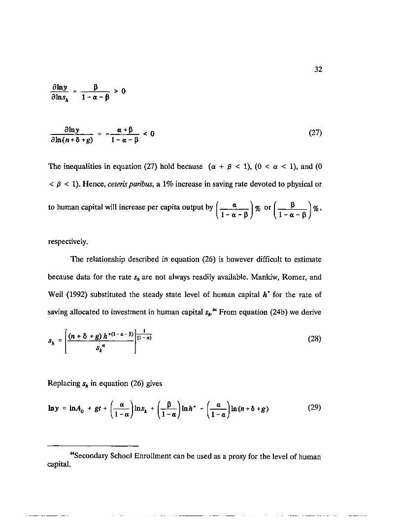
II. Steady State: A Graphical Representation

In the Solow model, the economy converges toward a steady state equilibrium,

where output, capital, and labor grow at the same rate n. As such, per capita output

and the capital-labor ratio are constant. The steady state equilibrium occurs at point

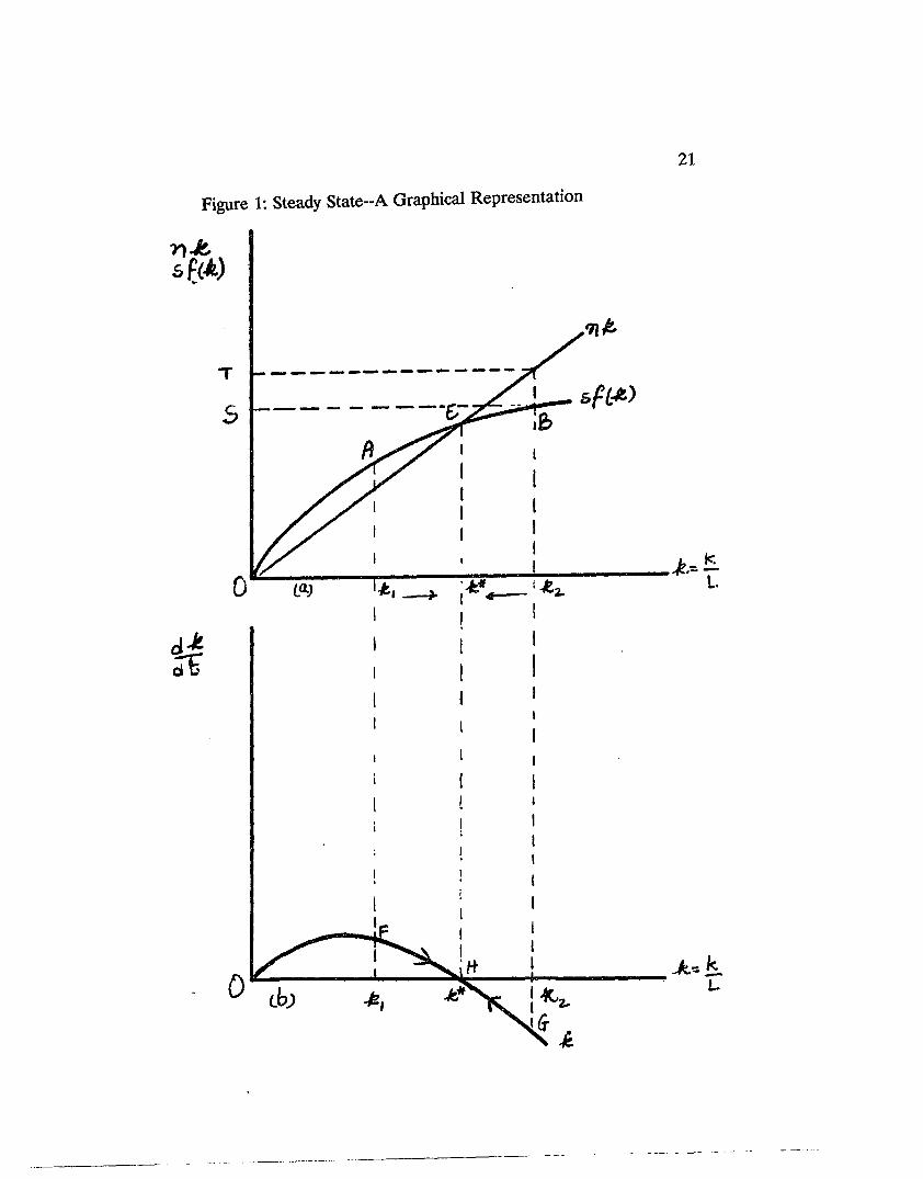
E in figure 1(a), corresponding to the capital-labor ratio k*.

The line nk in figure 1(a) is a linear function of k. It represents investment per

worker required to equip a labor force growing at rate n while maintaining a

constant capital-labor ratio. Along nk, the capital-labor ratio is constant.

The curve sf(k) in figure 1(a) represents saving per worker at various levels

of the capital-labor ratio. The function increases at a decreasing rate because of the

neoclassical assumption of diminishing returns.

The curve £ in figure 1(b) is the phase line. It represents the vertical distance

between sf(k) and nk. The shape of the phase line shows the path that capital

formation must follow to ensure full employment of inputs at a constant capital-labor

ratio.

Unlike the Harrod-Domar model, the economy here converges toward a stable

equilibrium, irrespective of whether it starts above or below the steady state capital-

labor ratio. For example, if the economy is below equilibrium E, say at point A,

saving per worker exceeds investment per worker necessary to maintain a constant

2 0

capital-labor ratio. The excess saving is represented by point F in figure 1(b), where

the change in capital stock is positive. Since saving strictly equals investment in this

21

Figure 1: Steady State--A Graphical Representation

s M

£

0 m

2 2

model, capital accumulation occurs as the economy continues investing in capital

stock. Hence the capital-labor ratio increases and the economy moves toward k*,

where k ‘ > k,.

Conversely, if the economy is above equilibrium E, say at point B, saving per

worker (OS) falls short of the amount of investment per worker (OT) required to

maintain a constant capital-labor ratio. The resulting shortage of capital is

represented by point G in figure 1(b), where the change in capital stock is negative.

Capital depletion occurs because the growth of the labor force exceeds the growth

of the capital stock. Hence, the capital-labor ratio falls from k2 toward k".

Once the economy reaches a capital-labor ratio of k m, the forces causing

change are in equilibrium. The economy is in steady state at point H (figure 1(b)),

where £ _ q. Therefore, the capital-labor ratio does not change, and ceteris paribus,

the economy experiences constant growth rates and constant living standard

indefinitely.

III. Predictions of the Solow Model

Two important results based on saving and population growth are derived

from Solow’s model. Equation (7) showed that the stock of capital per worker

increases over time with the saving rate and decreases with the labor growth rate. We

now individually analyze the impact of saving and population growth on economic

growth.

23

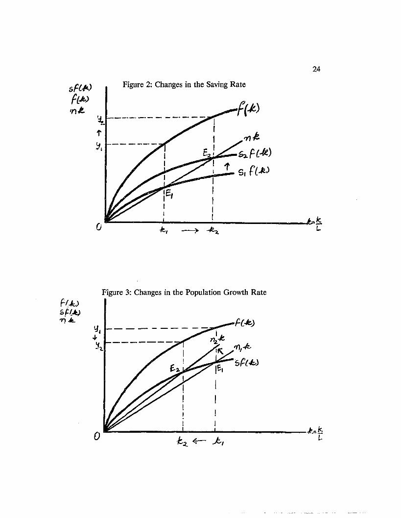
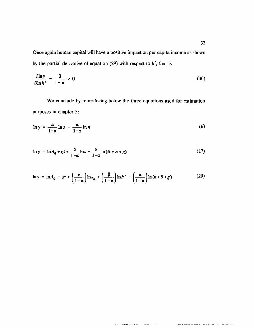
(a) Changes in the saving rate

One proposition of the Solow model is that, ceteris paribus, the higher the

saving rate, the higher the output per capita. This result is depicted in figure 2. With

an initial saving rate slf there is a steady state equilibrium at Et. The initial steady

state capital-labor ratio is kx and the resulting output per capita is aXy,.

Let the saving rate increase to s2 (where s2 > s2). The new steady state

equilibrium is at E2. At the new capital-labor ratio k* per capita output is now y*

which is greater than yv The higher saving rate makes more capital accumulation

possible. Per capita income therefore increases because output is a direct positive

function of capital.

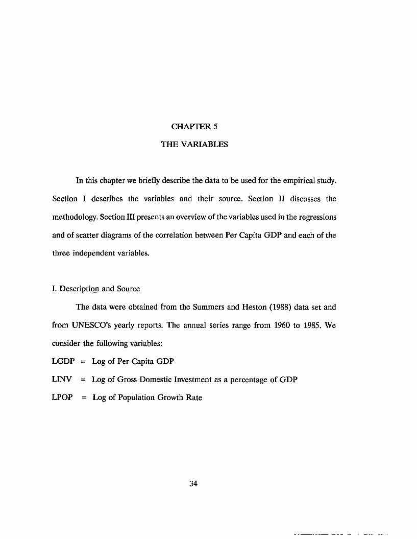
(b) Changes in the rate of population growth

The other proposition of the Solow model is that, ceteris paribus, the higher

the population growth rate, the lower the output per capita. As figure 3 shows, an

increase in population growth rate from nt to n2 results in a new investment line njc.

The capital-labor ratio decreases from kt to kr Output falls fromy, toy2 as the steady

state equilibrium moves from Ex to E2.

The model shows that an increase in population in excess of saving available

to support a constant capital-labor ratio results in capital depletion. Therefore, the

capital-labor ratio falls, as does the marginal product of capital. Hence, total output

and output per capita also falls.

24

Figure 2: Changes in the Saving Rate

----- >

Figure 3: Changes in the Population Growth Rate

CHAPTER 4

THE EMPIRICAL MODEL

In the previous chapter we examined the basic predictions of Solow’s model.

However, for econometric estimation purposes, we need to set up the proper

functional form that will allow us to determine the sign and magnitude of the effects

of saving and population growth on per capita income. The Cobb-Douglas production

function is a convenient functional form used in most empirical growth literature.

This chapter follows the specification of Solow’s basic model derived by Mankiw,

Romer, and Weil (1992). The incorporation of technology, depreciation, and human

capital into Solow’s model by Mankiw et. al. (1992) is shown in sections II and III.

I. Specification of the Basic Solow Model

The Cobb-Douglas production function takes the form

where a and (1 - a) represent the share of capital in income and the share of labor

in income, respectively. The Cobb-Douglas production function is linearly

homogeneous. Therefore we write equation (1) as

Y = F(K, L) = KaLl' a (0 < a < 1) (1)

(2)

25

Combining equation (2) above and equation (7) of chapter 3 and

simplifying35 yields

lny = —— Ins - —— Inn (6)1-a 1-a

which partially differentiated gives

> 001ns 1 -a

< o (7)31n n 1 -a

Equation (6) shows that, ceteris paribus, a 1% increase in saving rate will increase per

capita output by [ ? _ | %, whereas a 1% increase in population growth rate will1 1 - a J

decrease per capita output by f ] %. If the share of capital in income (a) is\ 1 - a J

roughly one-third, the model predicts an elasticity of per capita income of

“See Appendix A.

27

approximately .5 with respect to saving rate and approximately -.5 with respect to

population growth rate.36

II. Accounting for Technology and Depreciation

The predictions of the model discussed in chapter 3 were based on the

assumption of no technological progress. We saw that an economy follows a time

path of capital formation that relentlessly leads toward steady state. In steady state,

output per capita remains indefinitely constant. In order to understand observable

increases in standard of living, we will here relax this assumption. The section will

use Solow’s model to account for the impact of technological growth and

depreciation.

Consider the labor-augmenting production function

We assume that labor and technology grow exogenously at rates n and g respectively,

that is

“ De Long and Summers (1991) found a GDP growth elasticity of one-third percentage point with respect to machinery and equipment investment for the period

Y = F(K,AL) = Ka(AL)la

which is written as _ = f(k) = ka (8)

(9)

(10)

1960-1985.

28

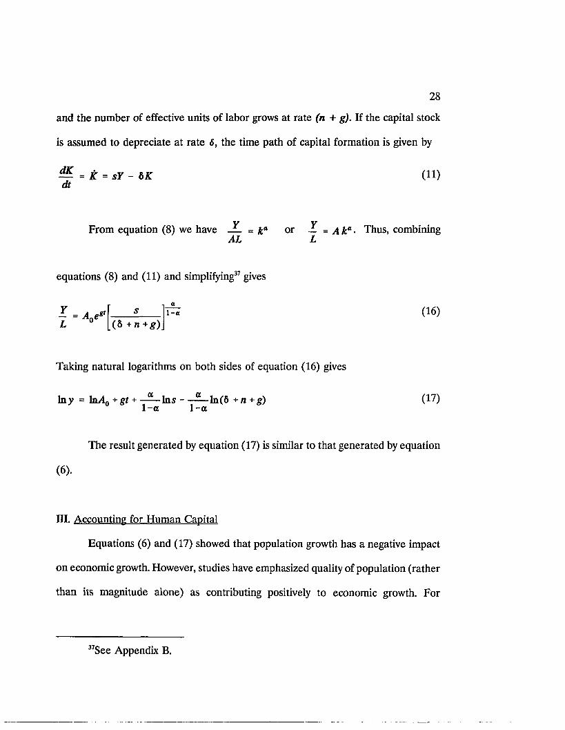
and the number of effective units of labor grows at rate (n + g). If the capital stock

is assumed to depreciate at rate 6, the time path of capital formation is given by

— = K = sY - bK (11)dt

Y YFrom equation (8) we have _ = or ~ = A ka- Thus, combimngAl* L

equations (8) and (11) and simplifying37 gives

s (16)y¥ = Ane*L 0 (8 +n+g)

Taking natural logarithms on both sides of equation (16) gives

lny = InA, +gt + In s ln(6 +n+g) (17)1-a 1-a

The result generated by equation (17) is similar to that generated by equation

(6).

III. Accounting for Human Capital

Equations (6) and (17) showed that population growth has a negative impact

on economic growth. However, studies have emphasized quality of population (rather

than its magnitude alone) as contributing positively to economic growth. For

37See Appendix B.

29

example, a study by Azariadis and Drazen38 (1990) found that a "highly literate

labor force" was crucial to rapid growth in the postwar period. Also, Lucas (1993)

emphasizes the role of a highly educated population in the economic success of East

Asian economies. Therefore, from an empirical point of view, failure to account for

human capital may result in specification bias. Furthermore, from a theoretical point

of view, if returns to all reproducible capital are constant (that is, if a + (3 = 1),

steady state is not possible in this model.39

In this section, we use the augmented Solow model developed by Mankiw et

al. to examine the importance of human capital.40 The augmented model expands

on the general production function described earlier by including human capital as:

Y = F(K,H,AL) (18)

where H is the stock of human capital. We retain all previous assumptions, but

modify the saving rate as follows:

(i) sk is the fraction of income invested in physical capital;

(ii) sh is the fraction of income invested in human capital.

^Azariadis, C., and A. Drazen, "Threshold Externalities in Economic Development," Quarterly Journal of Economics. 1990, p. 501-26.

39See Lucas (1988) and Mankiw et al. (1992).

““Mankiw et al. report that the Solow model accurately predicts the signs of the variables, but not their magnitude. In the endogenous literature this is attributed to the fact that the impact of human capital is more than traditionally accounted for (that is, where a = 0.3 and human capital is included in labor). See Mankiw (1992), p. 89, and Mankiw et al. (1992). Therefore, Mankiw et al. introduce human capital into the model to adjust for a possible specification error.

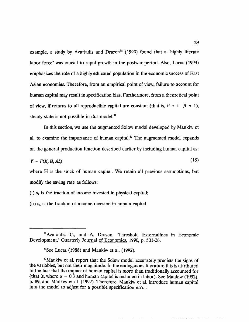
We further assume that the cost of producing a unit of human capital, physical

capital, or consumer good is the same. Also, we assume that human capital and

physical capital depreciate at the same rate 6.41

The Cobb-Douglas production function in this model can therefore be written

as:

where (a + /3 < 1), that is, decreasing returns to all capital occurs. The production

function can be expressed per effective unit of labor as

Changes in physical and human capital stocks can be written as

Y = KaH*ALll-a-V ( 0 <P <1 ) (19)

y = f(k, h, 1)

y = kah* (20)

where y = — , k = — AL AL

, and h = — AL

— = /. = s.Y - bK * *dt(21a)

dt(21b)

41We follow similar assumptions made by Mankiw et al. The two depreciation rates are assumed equal for purposes of algebraic simplification.

31

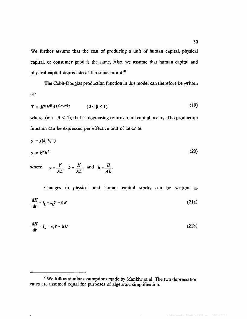
We use equations (20), (21a), and (21b) to derive42 the relationship between the

stocks of physical and human capital and saving and population growth rates as

k =n + 6 +g

( 1 - 0 - P ) (24a)

h =n + 6 +g

(1-0-p) (24b)

Equations (24a) and (24b) show that the stock of physical and human capital

varies directly with saving rate, and inversely with depreciation and the rate of

population growth.

The effect on per capita income can be examined by replacing equations (24a)

and (24b) into equation (20). Upon simplification43 we obtain

in * - b u . . p ♦ ' ( l ^ p ) to (" * s +g) (26)

Equation (26) above shows that per capita income varies positively with the fraction

of income invested in physical and human capital, and negatively with population

growth. Partial differentiations of equation (26) gives

iia . = « >o1 - a - p

““See Appendix C for derivations.

43See Appendix D.

32

B— > 0dln.sA 1 - a - p

< o (27)dln(/i + 8+g) 1 - a - p

The inequalities in equation (27) hold because (a + /3 < 1), (0 < a < 1), and (0

< /J < 1). Hence, ceteris paribus, a 1% increase in saving rate devoted to physical or

respectively.

The relationship described in equation (26) is however difficult to estimate

because data for the rate sh are not always readily available. Mankiw, Romer, and

Weil (1992) substituted the steady state level of human capital h ’ for the rate of

saving allocated to investment in human capital s*.44 From equation (24b) we derive

to human capital will increase per capita output by( 1 - a - p

a % or

_ (n + 6 +g)h*il~a~M (i-a) (28)

Replacing s„ in equation (26) gives

lay = ln̂ 40 + gt + ln(« + 8 +g)l - a )

(29)

“̂Secondary School Enrollment can be used as a proxy for the level of human capital.

33

Once again human capital will have a positive impact on per capita income as shown

by the partial derivative of equation (29) with respect to h*, that is

-®!22L. - L . > 0 (30)d ) n h * 1 -a

We conclude by reproducing below the three equations used for estimation

purposes in chapter 5:

lny = a In5 - ■■■ a Inn (6)1-a 1-a

lny = ln/l0 +gt + — — Ins - — — ln(6 + n +g) (17)1-a 1-a

lny = liu40 + gt+ ^ y^ -jln ^ + ^-^-jln^i* - ^ -7^-jln(w + 5 +8) (29)

CHAPTER 5

THE VARIABLES

In this chapter we briefly describe the data to be used for the empirical study.

Section I describes the variables and their source. Section II discusses the

methodology. Section III presents an overview of the variables used in the regressions

and of scatter diagrams of the correlation between Per Capita GDP and each of the

three independent variables.

I. Description and Source

The data were obtained from the Summers and Heston (1988) data set and

from UNESCO’s yearly reports. The annual series range from 1960 to 1985. We

consider the following variables:

LGDP = Log of Per Capita GDP

LINV = Log of Gross Domestic Investment as a percentage of GDP

LPOP = Log of Population Growth Rate

34

35

LPGD = Log of Augmented Population Growth Rate45

LSEC = Log of Secondary School Enrollment Ratio.

The lack of continuous series limited the study to 32 SSA countries.46 We consider

a cross-sectional-cum-time-series data set of 827 observations.47

II. Methodology

There are several ways to organize time-series-cum-cross-country data. The

following two methods are particularly common:

(i) testing individual time series for each country, and

(ii) averaging each country’s series into one data point and estimating a single cross-

sectional equation.48

The first method is useful when looking at conditions that influence growth

within individual countries over time because it makes use of all available data in the

series. However, the presence of data gaps may pose problems concerning the

reliability of the estimates.

45POP is augmented by .05 to account for depreciation and technology. Mankiw et al.’s assumption that (5 + g = .05) is based on studies that observed a value for depreciation of about .03 and for growth in per capita income of about 0.022.

““See Appendix H for a list of SSA countries considered.

47The statistical program used is MicroTSP version 7.0 by D. M. Lilien (1990).

"“Grier, K. B., and Tullock G., "An Empirical Analysis of Cross-National Economic Growth, 1951-80" Journal of Monetary Economics. 1989, p. 259-276.

36

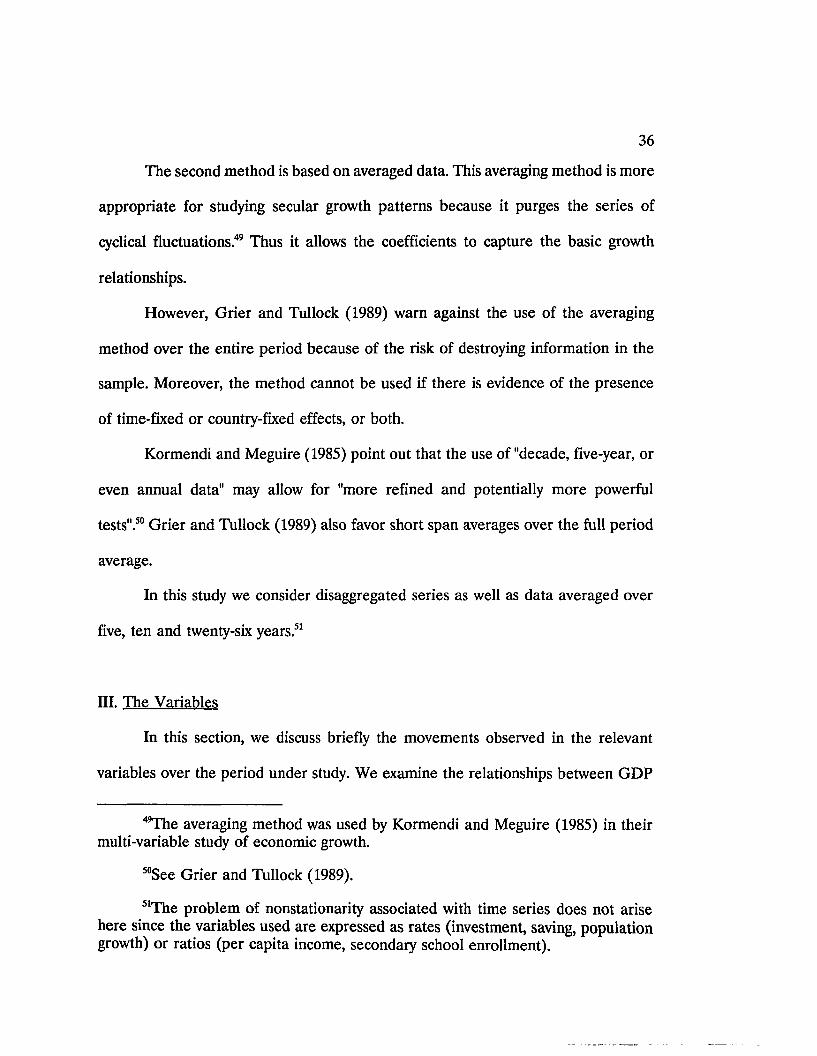
The second method is based on averaged data. This averaging method is more

appropriate for studying secular growth patterns because it purges the series of

cyclical fluctuations.49 Thus it allows the coefficients to capture the basic growth

relationships.

However, Grier and Tullock (1989) warn against the use of the averaging

method over the entire period because of the risk of destroying information in the

sample. Moreover, the method cannot be used if there is evidence of the presence

of time-fixed or country-fixed effects, or both.

Kormendi and Meguire (1985) point out that the use of "decade, five-year, or

even annual data" may allow for "more refined and potentially more powerful

tests".50 Grier and Tullock (1989) also favor short span averages over the full period

average.

In this study we consider disaggregated series as well as data averaged over

five, ten and twenty-six years.51

III. The Variables

In this section, we discuss briefly the movements observed in the relevant

variables over the period under study. We examine the relationships between GDP

49The averaging method was used by Kormendi and Meguire (1985) in their multi-variable study of economic growth.

50See Grier and Tullock (1989).

5IThe problem of nonstationarity associated with time series does not arise here since the variables used are expressed as rates (investment, saving, population growth) or ratios (per capita income, secondary school enrollment).

37

and the independent variables as portrayed in scatter diagrams.52 We also mention

any problem involved in using some of the variables.

A. The Dependent Variable

The trend in the growth of GDP in SSA over the past decades has been a

main cause for concern. In the 1980s, per capita income in SSA grew at an average

rate of -2.6% annually. This stands in sharp contrast with SSA’s post-independence

performance, when GDP grew at 2.0% on average annually. Also, such performance

contrasts with South Asia’s over those three decades. In the late 1960s-early 1970s,

South Asia was experiencing on average a 1.2% growth in per capita income. Two

decades later, its growth rate had increased to an annual average of 2.8%.

However, it is worth noting that the per capita GDP growth experience in SSA

has been varied at the individual country level. Between the 1960s and 1980s,

Botswana’s per capita GDP more than doubled, while Zaire’s and Ghana’s decreased

by 31.9% and 29.5%, respectively. Gabon’s average annual per capita GDP of

$3152.67 in the 1980s contrasts with Tanzania’s $332.83.53

We now examine the movements in saving, population growth, and secondary

school enrollment rates in SSA between the 1960s and 1980s.

52See Appendix E for scatter plots for each decade.

53Comparisons are based on averages of Summers and Heston’s (1989) data.

38

B. The Independent Variables

The assumption of a closed economy in chapter 3 means that saving strictly

equals investment. In fact, the trends in saving and investment in SSA over the

period considered move in the same direction. Both saving and investment in SSA

increased in the 1970s relative to their 1960s levels: saving rose from about 17% to

about 19.4%, while investment rose from 15% to 20.6%.M In the 1980s, they both

fell relative to their 1970s levels: saving fell from about 19.4% to about 12.5%, while

investment fell from 20.6% to 15.9%.

However, the "aggregate result conceals a wide variety of experiences among

country groups"55 as well as within countries over time. For example, in the 1960s

Burkina Faso experienced a negative saving rate while Zambia’s was 43.97%.

Mauritania’s saving rate fell from 32.87% in the 1960s to 6.04% in the 1980s.

Lesotho showed negative saving rates for the three decades considered, although

investment rate was consistently positive over the same time span.56

54The rates of saving and investment are percentages of GDP. The levels of saving and investment were higher in SSA than in South Asia in the early 1970s. See World Bank (1989).

55Aghevli, Bijan B., et al., "The Role of National Saving in the World Economy" IMF Occasional Paper. 1990, no. 67.

56The consistently negative saving rate in Lesotho may be related to the fact that a considerable portion of its labor force is temporarily employed in South Africa and transfers part of its income to Lesotho. See "Lesotho: A Development Challenge" World Bank Country Economic Report. 1975, p. 16-17. It appears that countries like Burkina Faso and Lesotho, two net exporters of labor, will experience negative saving rates because a portion of income spent on consumption may not be reported as earned income.

39

The specification of the Solow model requires the use of natural logarithms

on all variables. The occurrence of negative saving rates would make the

computation impossible. We therefore substitute gross domestic investment for saving

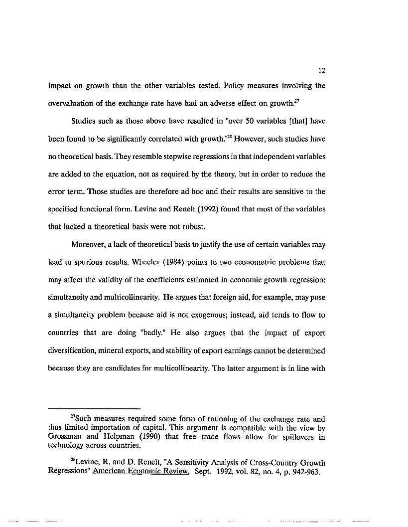
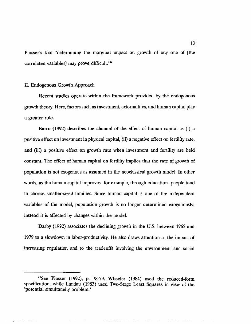
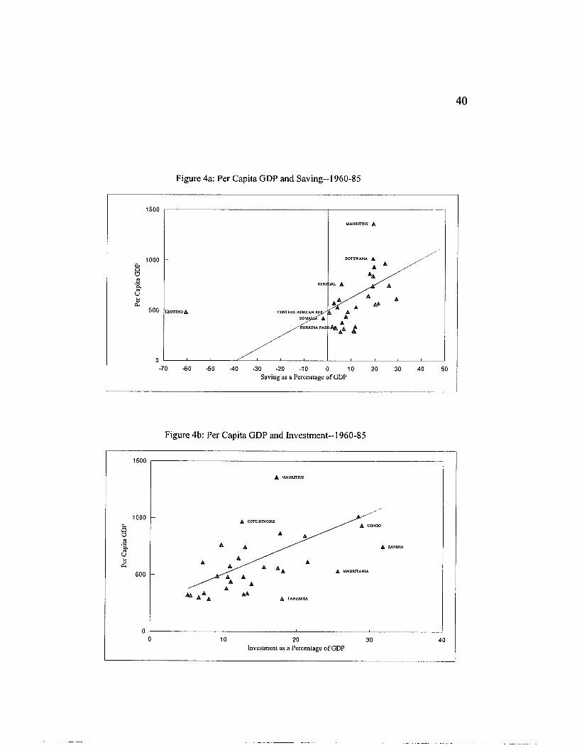
when regressing our two models.57 The scatter plots in figure (4a) and figure (4b)

show that both saving and investment are positively related to per capita GDP over

the period considered. Thus, the substitution of investment for saving in the

regressions will not severely alter the results.58 A positive coefficient on investment

will be consistent with the predictions of the model.

57See Appendix G for estimated coefficients when only positive saving rate is used, instead of investment rate. The empirical results based on saving rate are similar to regressions that use investment rate. Mankiw et al. (1992) also used Investment as a percentage of GDP in their regressions.

58The correlation coefficient between investment and saving is .42 on average over the study period. For the 1960s, 1970s, and 1980s, the correlation coefficient was .60, .40, and .24, respectively.

40

Figure 4a: Per Capita GDP and S aving-1960-85

1500

BOTSWANA A1000

500 EESOTHOA

^BURKINA FAS > ^

-70 -50 -40 -30 -20 -10 0 Saving as a P ercentage o f GDP

Figure 4b: Per Capita GDP and Investm ent-1960-85

1500

A MAURITIUS

1000A COTE DTVOIRB

A CONOO

A ZAMBIA

A MAURITANIA500

A TANZANIA

40Investm ent as a P ercentage o f GDP

41

The model also predicts a negative coefficient on population. Population

growth rate in SSA has been rising continuously since independence.59 In the late

1960s-early 1970s, population grew at 2.6% on average annually.60 In the late 1970s

and the 1980s, the growth rate amounted to 2.8% and 3.1%, respectively.

The observed population increases in SSA occur despite claims of declining

fertility rates. Although fertility rates fell by 26% in Botswana, 35% in Kenya, and

18% in Zimbabwe,61 for example, these countries experienced population growth

rates in excess of 2% on average over the past three decades. This can be due in

part to the growing number of women of reproductive age. It is argued that high

fertility rates in the early 1960s resulted in a lagged increase in the number of women

of childbearing age. Given persisting cultural patterns,62 this means that lower

fertility rates do not necessarily result in lower population growth rates.63

59In absolute terms, Africa’s population is not a concern, since the population density of SSA in 1987 was 21 persons per square kilometers compared with South Asia’s 210, East Asia’s 108, and Europe’s 34. (See World Development Report 1989). In fact, Odedokun (1993) found that population size promotes growth in Africa. However, relative to GDP growth and resource base, population growth in SSA poses a severe living standard problem.

“ World Bank (1989), Sub-Saharan Africa-From Crisis to Sustainable Growth.p 26.

61See Robey et al. (1993).

“Cultural patterns affect, for example, the age at marriage of women, the number of spouses.

63It is also necessary to look at the movement in birth and death rates: there was a notable fall in the death rate in SSA between 1965 and 1987, while the fall in the birth rate during that same period was minor. Moreover, infant mortality rates for 1965, 1975, and 1987 displayed a downward trend in low-income and middle- income economies. See World Bank (1989), World Development Report.

42

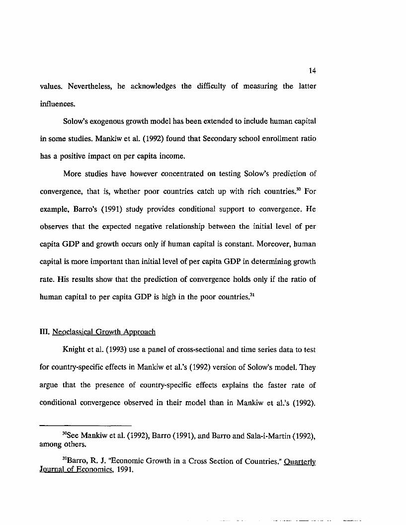
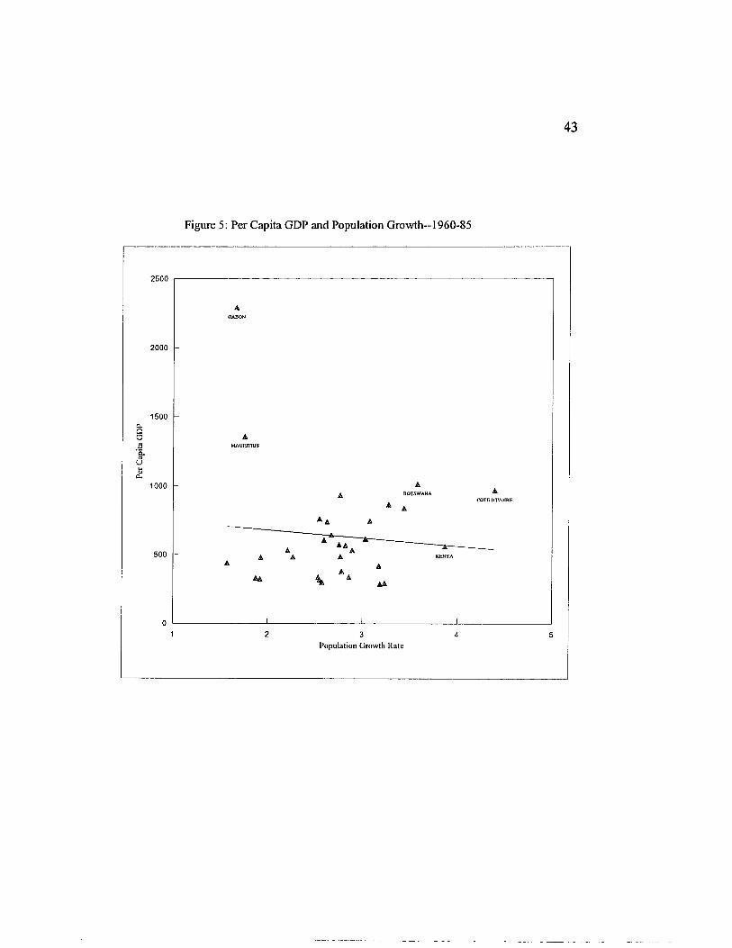
SSA’s steadily growing population adds more and more people to its pool of

workers. Relative to resource base, population growth leads to a fall in the marginal

productivity of labor. Hence, per capita output fall. As shown in figure (5), there is

a negative relationship between population growth and per capita GDP in SSA over

the 1960-80 period.

43

Figure 5: Per Capita GDP and Population Growth--1960-85

2500

2000

1500CUQoBE.«u1000

500

1 2 3 4 5Population G rowth Rate

44

The third model of this study analyses the impact of investment in human

capital. The concept of human capital is related to changes in the quality of labor.

Secondary school enrollment is generally used as a measure of the quality of

manpower. However, even when data on enrollment in secondary education is

available, caution must be taken in its use. Schultz (1988) warns that the impact of

education on productivity is based on "populations in which educational attainment

is not randomized but is itself an economic choice variable."64 Moreover, a measure

of the concept of human capital is not comparable to a measure of physical capital

because of the particular features of the former. Schultz lists four of those features.

First, property rights apply differently to human capital and to physical capital.

Second, worker preferences are involved in human capital. Third, non-marketable

goods are affected by education but are not measurable. And finally, welfare effects

arise because the benefit of an improvement in human capital is shared by the

community.65

Enrollment in secondary education in SSA improved from 4% in 1965 to 16%

in 1986.66 This movement was similar to the trend in secondary education worldwide

over that same period. Moreover, Africa (along with East Asia) was considered

“Schultz, T. P., "Education Investment and Returns" in Handbook of Development Economics vol. 1, by Hollis Chenery and T. N. Srinivasan, 1988.

“ Ibid

66The numbers refer to the percentage of people within the secondary schooling age group actually enrolled in secondary education. The measure of enrollment is weighted according to each country’s share in SSA population. See World Development Report (1989).

45

among the "overachievers," in contrast with South Asia, West Asia, and Latin

America, where investment in education was lower than expected.67

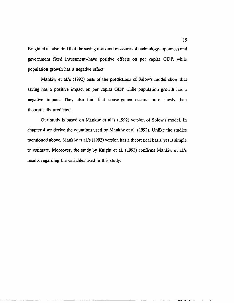
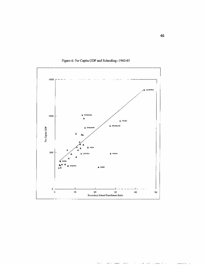
The augmented model predicts a positive coefficient on schooling. The scatter

diagram in figure (6) shows that schooling is positively related to per capita GDP in

SSA between the 1960s and 1980s.

67See Schultz’ (1988) framework.

46

Figure 6: Per Capita GDP and Schooling--1960-85

1500

A BOTSWANA1000

A CONOO

A SWAZILANDA ZIMBABWE

A TOOO

500 A GHANA

A ZAIRE

00 10 20 30 40 50

Secondary School E nro llm en t Ratio

CHAPTER 6

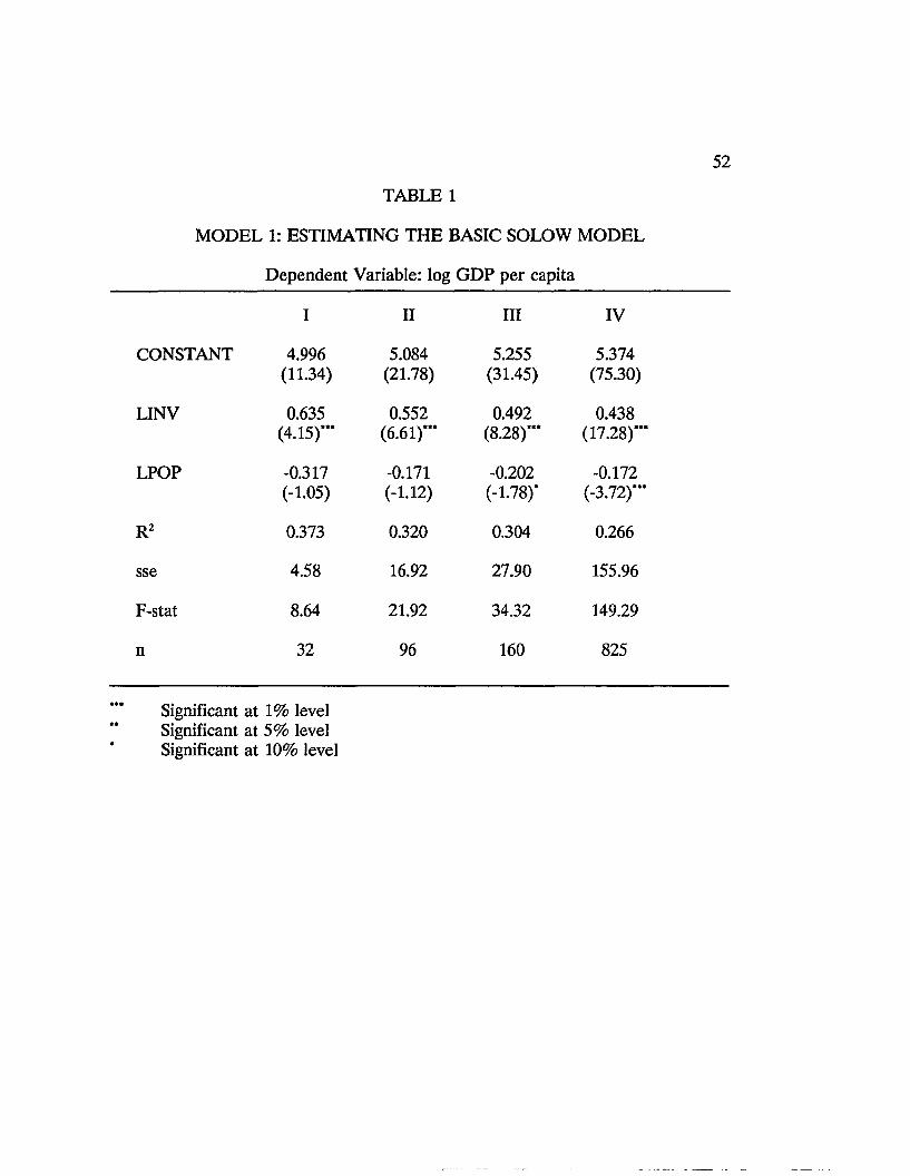
ESTIMATION PROCEDURE AND RESULTS

In this chapter we discuss the empirical results. The basic Solow predictions

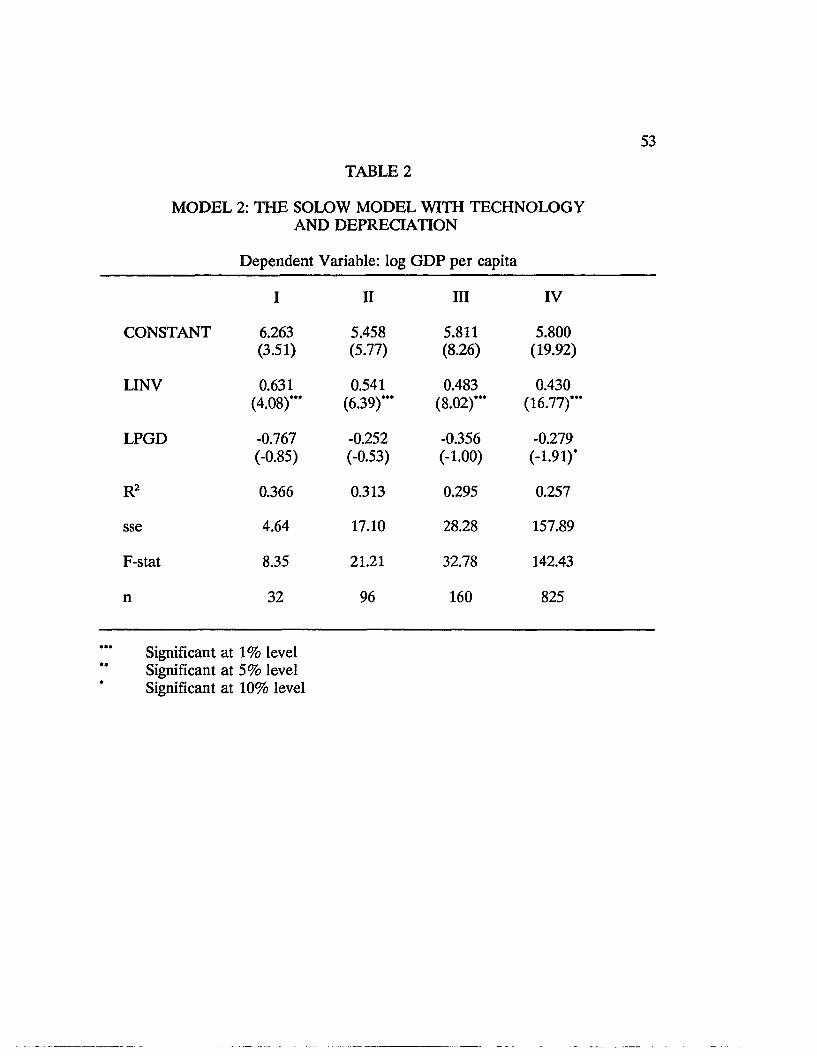
are tested in Model 1 which is based on equation (6) of chapter 3. Model 2 augments

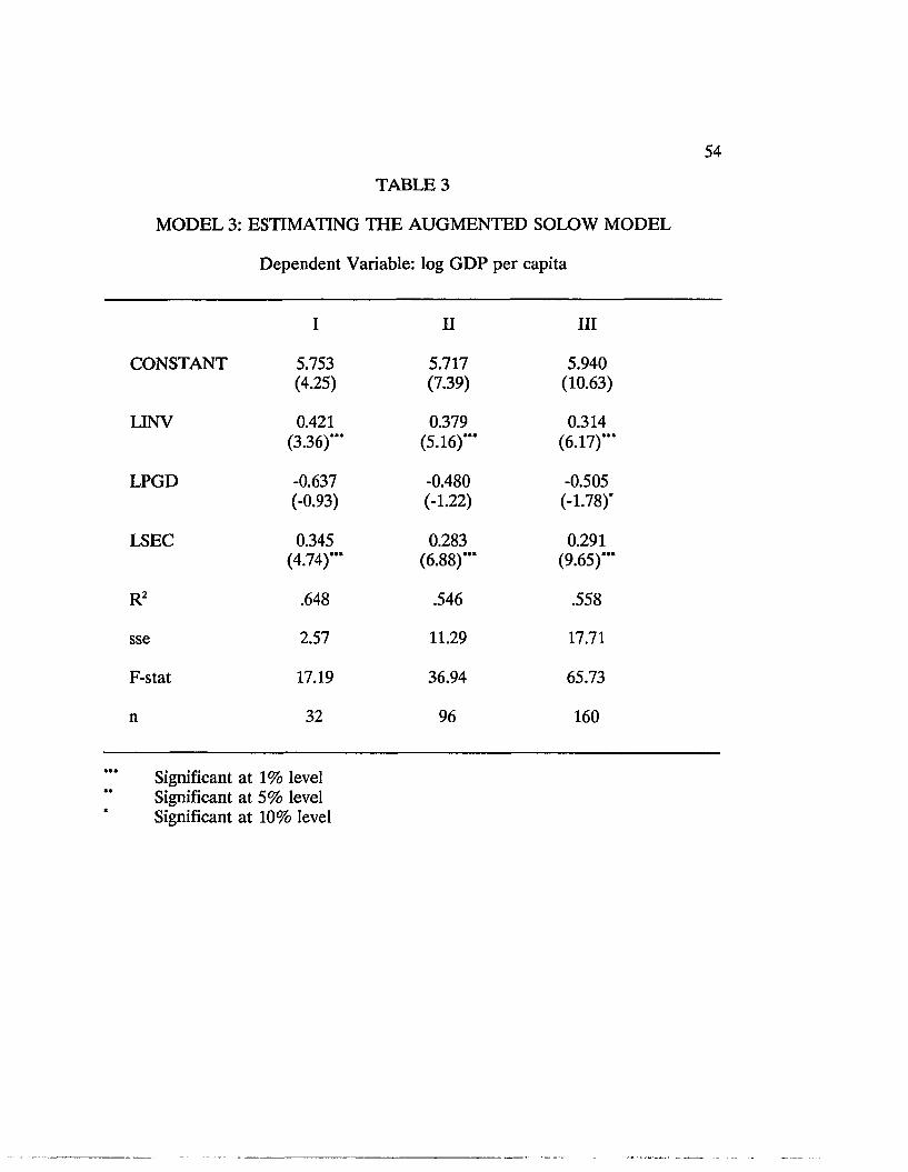
population by 0.05 to account for depreciation and technology. The effect of human

capital is tested in Model 3 which is based on the augmented equation (29) of

chapter 4.

LGDP = CONSTANT + a^UNV - a2LPOP (MODEL 1)

LGDP = CONSTANT + ^ 1UNV - P2LPGD (MODEL 2)

LGDP = CONSTANT + y l LINV - y2LPGD + y^LSEC (MODEL 3)

Positive coefficients on LINV and LSEC would be consistent with Solow’s predictions

and with Mankiw et al.’s (1992) results. The basic Solow model also predicts a

negative coefficient on LPOP. Model 1 and Model 2 appear in Tables 1 and 2,

respectively. They each consist of four regressions of differing levels of

aggregation.68 The first regression pools the 32 African countries over a period of

“We regressed dummy variables to test for shifts over time and across countries. The results showed no shift in the intercept due to time. Country dummies for only Liberia, Togo, and Zambia were not significant. However, LPOP was positive and significant in the latter regression.

47

48

26 years.69 The second regression pools three decadal averages for each of the 32

countries, amounting to 96 observations. The third regression of 160 is a pooling of

five quinary averages per country. The fourth regression uses 827 observations, being

a panel of 26 annual data points for the 32 countries.70

Model 3 is shown in Table 3. It is tested using three regressions similar to the

first three used in Models 1 and 2. Due to unavailability of continuous data on

secondary school enrollment in SSA over the period studied, it was not possible to

perform regression using annual panel data.71

We observe that the significance of the variables improves with the level of

disaggregation.72 Both investment and secondary school enrollment are significant

at 1% level in their respective regressions. Population growth is significant at 1%

level only in the fourth regression of Model 1 (when n = 825). Augmented

population growth is significant at 10% level in Model 2 only when n = 825.

The inclusion of secondary school enrollment, the proxy for human capital,

improves the significance of the augmented population growth variable slightly, such

69We use one data point per country.

70Data for Burkina Faso ranges from 1965 to 1985.

71Initial regressions of individual country data yielded no meaningful pattern. Regressions using averages for the 1960s, 1970s, and 1980s, respectively showed that investment was always positive and significant. However, population was never significant and was of the wrong sign in the 1980s.

^This is compatible with arguments by Grier and Tullock: they warn that highly aggregated series result in the loss of information generally present in raw data.

49

that the latter becomes significant at 10% level when n = 160 (in Model 3).73

However, when human capital is accounted for, the importance of physical capital

declines.74 The overestimation of the investment coefficient in Models 1 and 2

implies that physical capital and human capital are positively correlated. Also, we

note that the coefficient of determination (R2) in Models 1 and 2 falls as the data

becomes more disaggregated and the number of observations increases.75

The sign on investment is consistent with the basic Solow prediction, with

Mankiw et al.’s (1992) results and with other empirical literature on economic

growth.76 Our results show that, in the case of SSA, saving has a significantly

positive impact on per capita GDP, in accordance with the findings of Knight et al.

(1993).77 Although the negative impact of population growth is compatible with the

73This observation seems compatible with Azariadis and Drazen (1990) who point out that the omission of a human capital variable may lead to a specification bias.

74The coefficient on LINV in the first three regressions is smaller in Model 3 than in Models 1 and 2. The inclusion of secondary school enrollment in Mankiw et al.’s regressions reduces the coefficient on investment.

75This may be due to increased variation in the dependent variable as the sample size increases from averaged decadal or quinary variations to annual variations.

76When setting up the basic Solow model in chapter 3, we assumed that saving equals investment.

^The coefficients are not stable over the time span considered: the size of the coefficients differs across each five-year period.

50

above-mentioned work, it is not consistently significant throughout our results.78

Secondary school enrollment has a significantly positive impact on per capita GDP.

Landau (1983) found that investment in education was positive and significant at 1%

level in cross-country regressions. Also, in Otani and Villanueva’s (1990) cross­

country regressions, "Budgetary share of expenditure on human capital" was positive

and significant at 10% level.

According to our results, education and high saving tend to promote growth.

This is consistent with Lucas’ (1993) observation that "miracle economies" are

characterized by an increasingly well-educated population and a high saving rate

among other features.

Although our models are similar in structure to Mankiw et al.’s (1992), there

are nonetheless differences between the two studies. On the one hand, Mankiw et

al.’s (1992) results are based on a heterogeneous sample of developed and developing

countries. In contrast, our work focuses on a particular group of developing countries:

Sub-Saharan Africa. On the other hand, Mankiw et al. (1992) use cross-sectional data

in their regressions, while the major portion of our findings is based on data that

78The decrease in significance when population growth is augmented may imply that the obsolescence effect on labor of technological progress does not hold for SSA.

51

involve cross-sectional as well as time series dimensions.79

In conclusion, we have shown that Solow’s predictions that saving has a

positive effect and population growth has a negative effect on per capita income hold

for SSA over the period studied. Investment and Secondary school enrollment are

consistently significant, whereas Population growth is significant only when a large

number of observations is used or when the model is augmented. Regressions using

the most disaggregate data set improve the significance of the variables. The results

are consistent with existing empirical literature on economic growth.

79In order to test the relevance of the approach developed by Mankiw et al. to a study of SSA countries, we used the coefficients estimated in Models 1 and 2 to predict per capita income in SSA for the 1980s. We found that the models do not accurately predict the level of per capita income for the five SSA countries used in the test. See Appendix F for comparisons between predicted and actual per capita income in SSA.

52

TABLE 1

MODEL 1: ESTIMATING THE BASIC SOLOW MODEL

Dependent Variable: log GDP per capita

I II III IV

CONSTANT 4.996(11.34)

5.084(21.78)

5.255(31.45)

5.374(75.30)

LINV 0.635(4.15)***

0.552(6.61)***

0.492(8.28)*"

0.438(17.28)***

LPOP -0.317(-1.05)

-0.171(-1.12)

-0.202(-1.78)*

-0.172(-3.72)***

R2 0.373 0.320 0.304 0.266

sse 4.58 16.92 27.90 155.96

F-stat 8.64 21.92 34.32 149.29

n 32 96 160 825

Significant at 1% level Significant at 5% level Significant at 10% level

53

TABLE 2

MODEL 2: THE SOLOW MODEL WITH TECHNOLOGY AND DEPRECIATION

Dependent Variable: log GDP per capita

I II III IV

CONSTANT 6.263(3.51)

5.458(5.77)

5.811(8.26)

5.800(19.92)

LINV 0.631(4.08)*"

0.541(6.39)***

0.483(8.02)***

0.430(16.77)***

LPGD -0.767(-0.85)

-0.252(-0.53)

-0.356(-1.00)

-0.279(-1.91)*

R2 0.366 0.313 0.295 0.257

sse 4.64 17.10 28.28 157.89

F-stat 8.35 21.21 32.78 142.43

n 32 96 160 825

Significant at 1% level Significant at 5% level Significant at 10% level

54

TABLE 3

MODEL 3: ESTIMATING THE AUGMENTED SOLOW MODEL

Dependent Variable: log GDP per capita

I II III

CONSTANT 5.753 5.717 5.940(4.25) (7.39) (10.63)

LINV 0.421 0.379 0.314(3.36)*** (5.16)*** (6.17)***

LPGD -0.637 -0.480 -0.505(-0.93) (-1.22) (-1.78)*

LSEC 0.345 0.283 0.291(4.74)*** (6.88)*** (9.65)***

R2 .648 .546 .558

sse 2.57 11.29 17.71

F-stat 17.19 36.94 65.73

n 32 96 160

Significant at 1% level Significant at 5% level Significant at 10% level

CHAPTER 7

CONCLUSION

In this study we have examined whether Solow’s predictions about the role of

saving and population growth in the determination of per capita income hold for

Sub-Saharan Africa (SSA). Our work was prompted by the growing concern over the

poor economic performance of SSA relative to the rest of the world over the past

decades.

We used Mankiw et al.’s (1992) version of Solow’s model to estimate pooled

cross-sectional-cum-time-series regressions on 32 SSA countries. Our results are

consistent with those obtained by Mankiw et al. (1992) and by Knight et al. (1993).

We found that, in the case of SSA, saving has a positive and significant impact on per

capita income. The impact of population growth on per capita income was

consistently negative, though significant only when the most disaggregate data was

used or when human capital was included. This population growth behavior is

compatible with arguments by Grier and Tullock (1989) and by Azariadis and Drazen

(1990).

Given the crucial assumptions of (i) variable factor proportions in a linearly

homogeneous production function, (ii) a closed economy, and (iii) equality between

55

56

saving and investment, steady state occurs. While the Solow model predicts the

direction of the impact of saving and of population growth, the long-run steady-state

phenomenon does not account for the observed growth slowdown. However, based

on our results, shifts in steady states-arising from the upward trend in population

growth and the downward trend in saving observed in SSA-have exerted a

continuous downward pressure on that region’s per capita GDP.

Hence, it appears that investment in physical capital and in human capital are

the most effective policy channels available to SSA to reverse the downward trend

in per capita income. In fact, we found that saving rate and secondary school

enrollment ratio are significant promoters of per capita income.

While panel results were according to expectations, estimations and

predictions using country time series suggested presence of misspecification errors.

However, it may be very difficult to address the latter issue in view of data

availability problems.

An extension to this work will involve comparisons between SSA and other

groups of developing countries. Particularly, it would be interesting to see how well

the Solow predictions fit more narrowly defined groups of countries such as Latin

America and Caribbean countries or South and East Asia. The results may provide

insight to the disparity between group and individual country performances observed

in this study.

APPENDICES

APPENDIX A

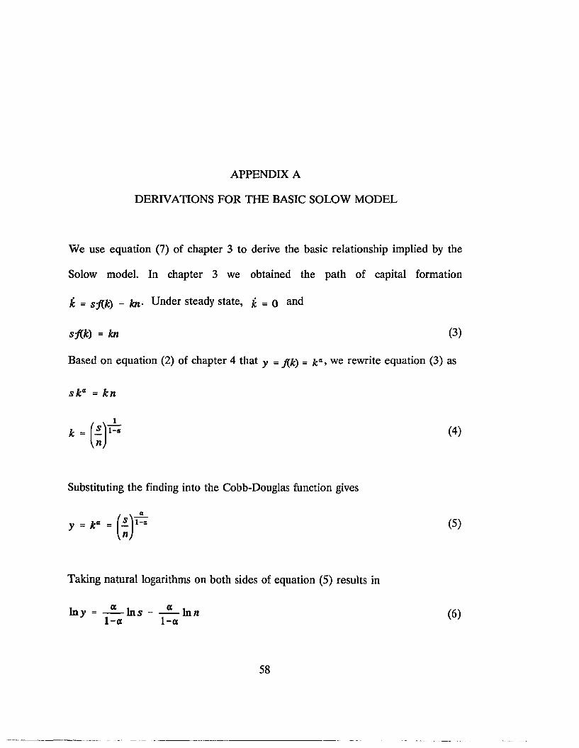
DERIVATIONS FOR THE BASIC SOLOW MODEL

We use equation (7) of chapter 3 to derive the basic relationship implied by the

Solow model. In chapter 3 we obtained the path of capital formation

k = s'ffl) - kn- Under steady state, £ = 0 and

s-J(k) = kn (3)

Based on equation (2) of chapter 4 that y = = £«, we rewrite equation (3) as

s k a = kn

k = (4)

Substituting the finding into the Cobb-Douglas function gives

y = ka = (5)

Taking natural logarithms on both sides of equation (5) results in

lny = —̂— Ins - —^-ln/t (6)1 - a 1- a K }

58

APPENDIX B

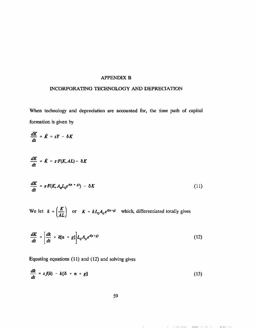
INCORPORATING TECHNOLOGY AND DEPRECIATION

When technology and depreciation are accounted for, the time path of capital

formation is given by

— = K = sY - 6K dt

= K = sF(K,AL) - 5 K

— = s-F(K,AQL0eKn + *>) - 5 K (11)

or K = kL0A0et('n+s) which, differentiated totally gives

(12)

Equating equations (11) and (12) and solving gives

— = sf(k) - fc[5 + n + g\ (13)

59

60

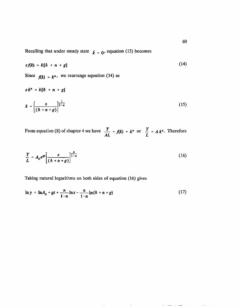
Recalling that under steady state fc = q, equation (13) becomes

sf(k) = fc[6 + n + g\

Since _ ^a, we rearrange equation (14) as

(14)

s k a = fc[6 + n + g]

k =(6 +n+g)

l1 - a (15)

From equation (8) of chapter 4 we have — = flk) = ka or X = A ka- ThereforeAL L

(6 +n+g)

a1 - a (16)

Taking natural logarithms on both sides of equation (16) gives

lny = ln/l0 +gt + —— Ins - —— ln(8 + n+g) 1-a 1-a

(17)

APPENDIX C

DETERMINING STEADY-STATE CAPITAL STOCKS

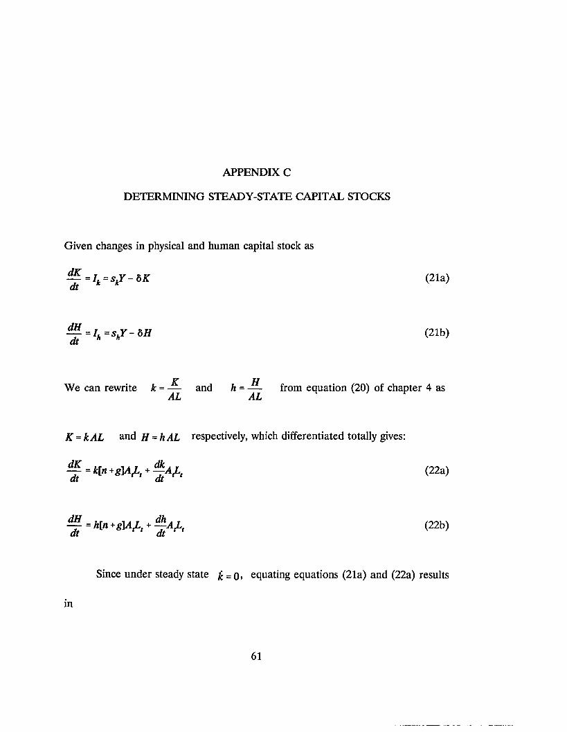
Given changes in physical and human capital stock as

(21a)

dHdt

= Ih =shY - b H (21b)

K HWe can rewrite k = — and h = — from equation (20) of chapter 4 asAL AL

K = kAL and H = hAL respectively, which differentiated totally gives:

+ (22a)

Since under steady state H = q, equating equations (21a) and (22a) results

in

61

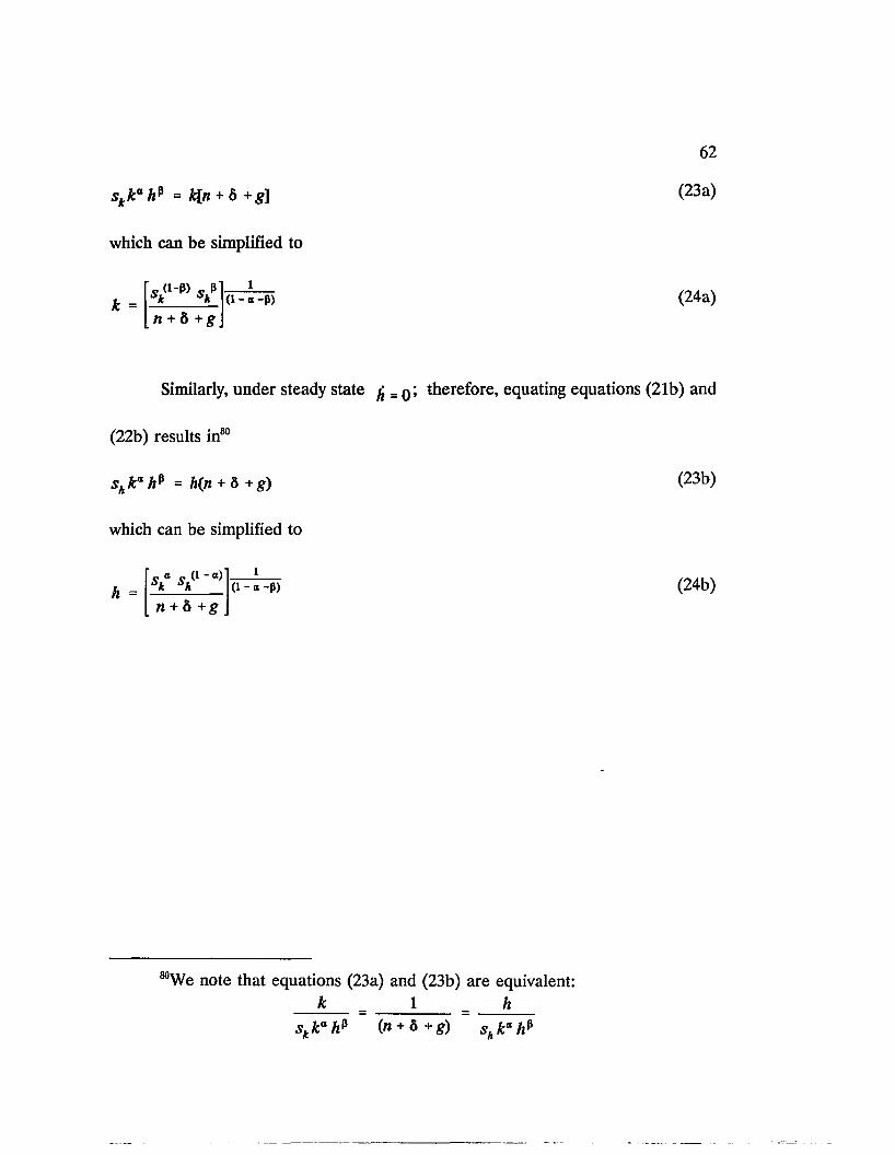
62

(23a)

which can be simplified to

k =( l - P ) c P

n + 6 + g

id - « - P ) (24a)

Similarly, under steady state ^ = therefore, equating equations (21b) and

(22b) results in180

s. ktt hp = h(n + b + g) (23b)

which can be simplified to

« c. (i - “ )

h = V sh ( 1 - a -P)

n + 6 +g(24b)

“ We note that equations (23a) and (23b) are equivalent:k = 1 = h

skkah.l (n + b+g) shkahp

APPENDIX D

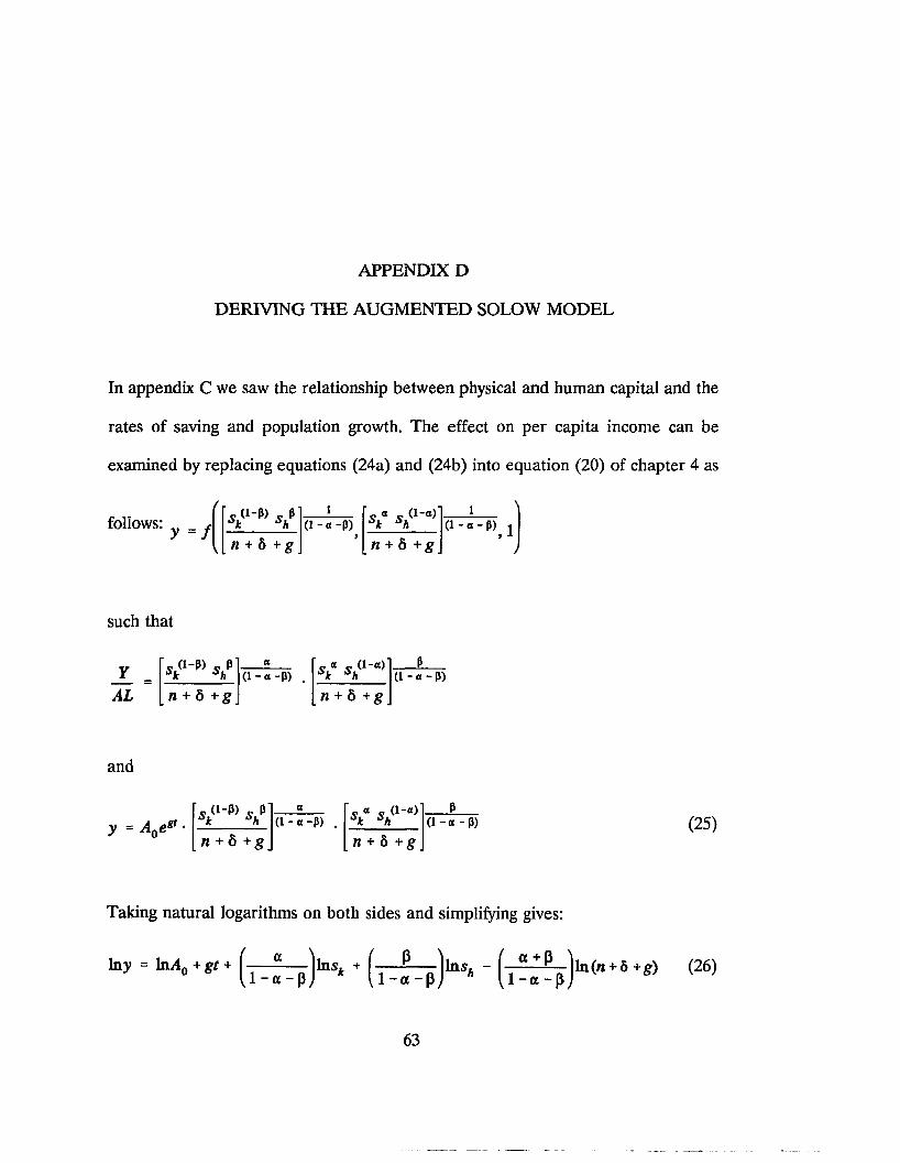
DERIVING THE AUGMENTED SOLOW MODEL

In appendix C we saw the relationship between physical and human capital and the

rates of saving and population growth. The effect on per capita income can be

examined by replacing equations (24a) and (24b) into equation (20) of chapter 4 as

follows: y = fl 1

&

1 i \(l-o —P)1 (1-o-P) ,9 1

/,[» + 5 +g_ n + 6 +g

such that

Y_AL

< i - P ) P

n + 6 + g( 1 - a -p) Sk Sh l ~a)

n + 6 + g( 1 - 0 - P )

and

y = A ^ 8* f y ' - 1” V Ia

k * k 1'*']p

d - « - P ) . ( 1 - o - P )

i t + 6 + g 71 + 6 + g(25)

Taking natural logarithms on both sides and simplifying gives:

In* - lnj40 + g r + ( Y r f r p ) 1™* + ( t ^ p H ■ ( i r ^ a ^ p ) ln<" + 6+S> (26)

63

APPENDIX E

RELATIONSHIPS BETWEEN THE INDEPENDENT VARIABLES

AND PER CAPITA GDP

The scatter diagrams for the 1960s, 1970s, and 1980s show the relationship

between per capita GDP and saving, investment, schooling, and population growth

separately.

As expected, there is a consistently positive relationship between per capita

GDP and saving, investment, and schooling for each decade.

The scatter plots show an expected negative relationship between per capita

GDP and population growth for the 1960s and 1970s. The positive fit shown for the

1980s may be related to major economic and political disturbances in SSA in that

decade.

64

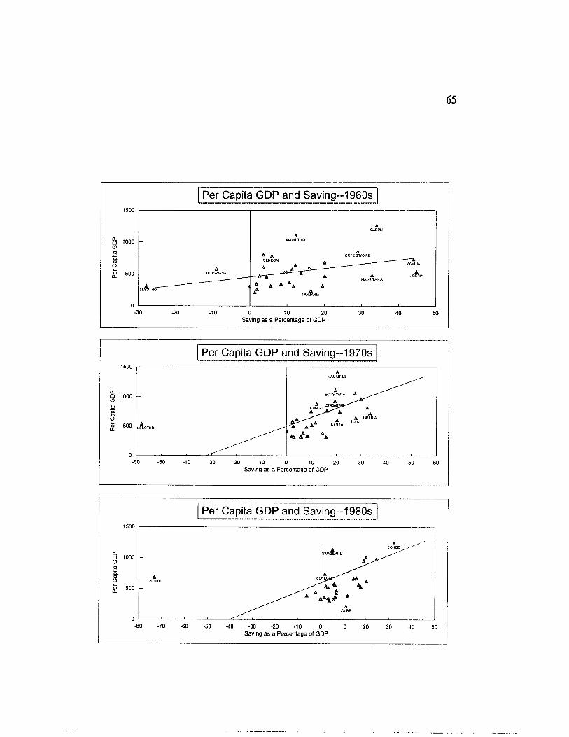
65

Per Capita GDP and Saving-1960s1500

1000

500

-30 -20 -10 40Saving P e rc e n ta g e of GD P

Per Capita GDP and Saving-1970s1500

Q 1000 0(0Q .sa)

a . 500

-60 -50 -40 -30 -20 -10 0 10 S aving a s a P e rc e n ta g e of GDP

20 30 40 50 60

Per Capita GDP and Saving-1980s1500

1000

500

0-70 -60 -50 -40 -30 -20 -10 0 10 20 30 40 50

S aving a s a P e rc e n ta g e of GDP

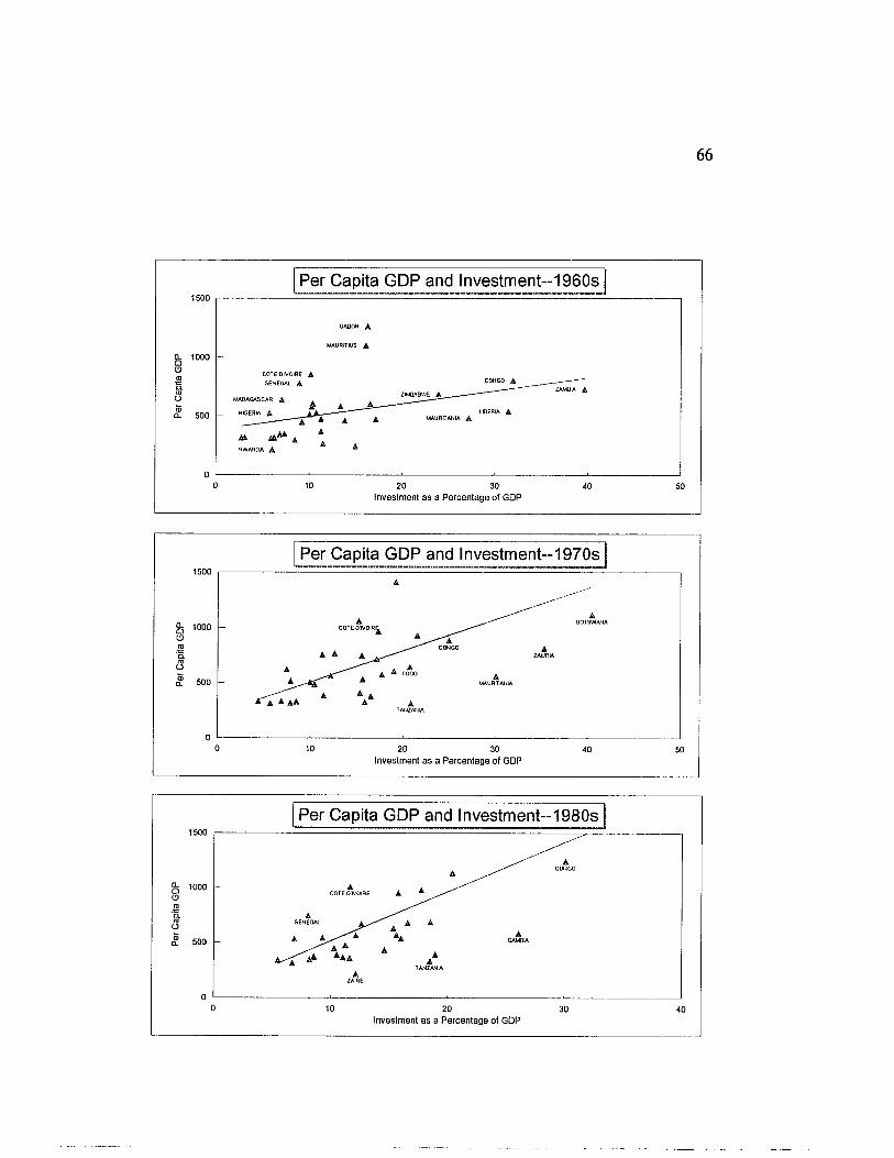
66

Per Capita GDP and Investment--1960s1500

GABON A

Q- 100 0

COTE O'fVOlRE A SENEGA! A CONGO A

ZAMBIA A

MADAGASCAR A

IGERIA ANIGERIA A500 MAURITANIA A

RWANOA A

20 30Investm en t a s a P e rc e n ta g e of GDP

Per Capita GDP and Investment-^970s1500

1000

500

40Inv estm en t a s a P e rc e n ta g e of GDP

Per Capita GDP and lnvestment--1980s1500

1000

500

kAA

20Inv estm en t a s a P e rc e n ta g e of GDP

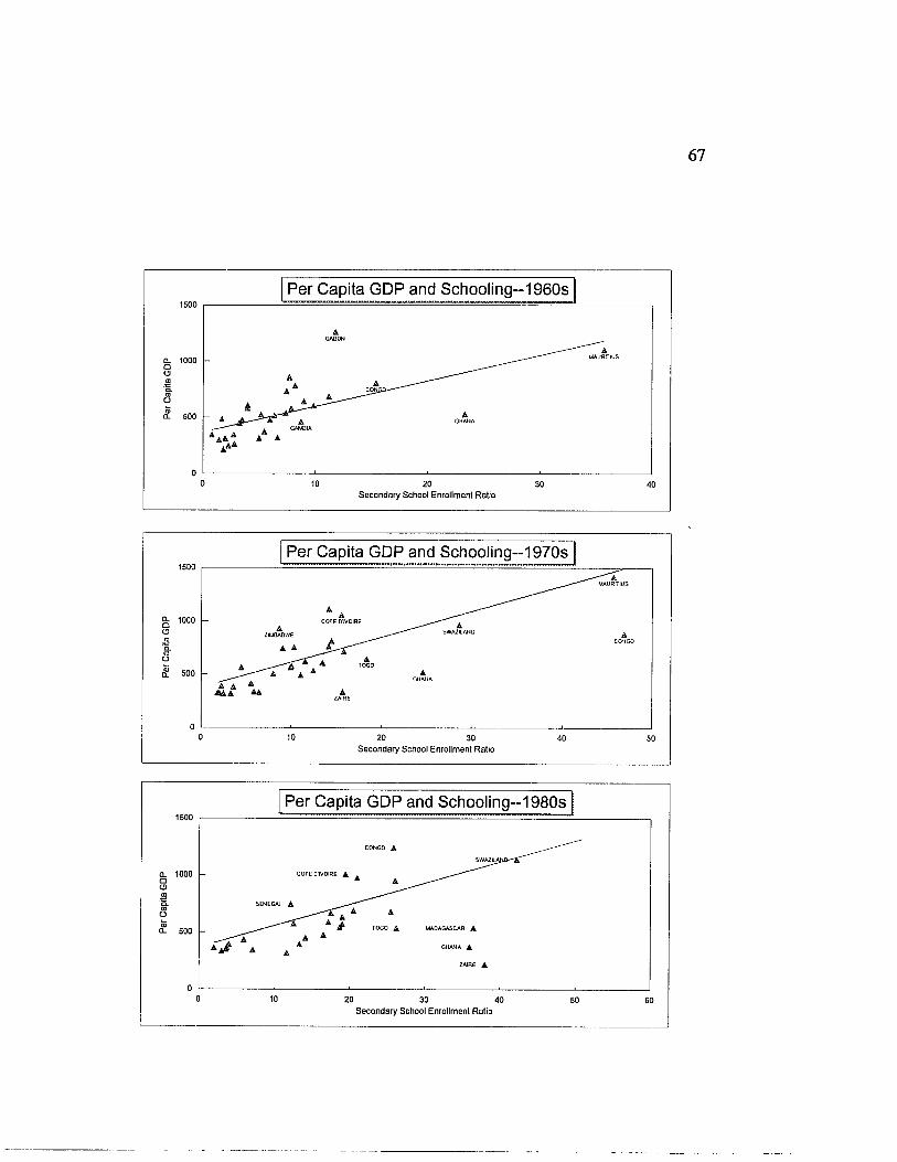
67

Per Capita GDP and Schooling--1960s1500

c l 1 0 0 0

500

00 10 20 30 40Secondary School Enrollment Ratio

Per Capita GDP and Schooling-1970s1500

Or 1000

500

Secondary School Enrollment Ratio

Per Capita GDP and Schooling-1980s1500

CONGO A

CL 1000 COTE D'fVOIRE A

TOGO A MADAGASCAR A

S econdary School Enrollment Ratio

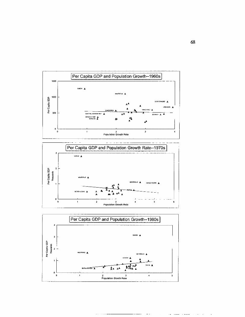
Per Capita GDP and Population Growth-1960s1500

a 1000aCDoj5.coOa>Q. 500

00 1 2 3 4

Population Growth Rate

COTE DWOKE A

/MOAIME ASWAZLAND A

-------- — ------tr~&—-* -■ ■*CENTRAiAfRCANREP A ^ A

SCRRALEONE A AABURUNDI A M " XA

Per Capita GDP and Population Growth Rate-1970s3

GABON A

2

1

00 21 3 4 5 6Population Growth Rate

Growth-1980s

MAURITIUS ABOTSWANA A

CONGO A

KENYA A

PURKN

Population Growth Rate

APPENDIX F

PREDICTIONS OF THE MODELS

We use coefficients estimated by the basic Solow model (Model 1) and by

Mankiw et al.’s version of the Solow model (Model 2) to calculate the estimated

growth rate of per capita income for Burkina Faso, Congo, Madagascar, Mauritius,

and Togo in 1980 and 1985. These countries were chosen because time series

regressions using their individual data yielded expected signs on the coefficients.

Population growth rate is augmented by 0.05 in Model 2 to account for

technology and depreciation. The estimated growth rates differ from the actual

growth rates. In some cases where the rates are of relatively similar magnitude, the

signs differ.

69

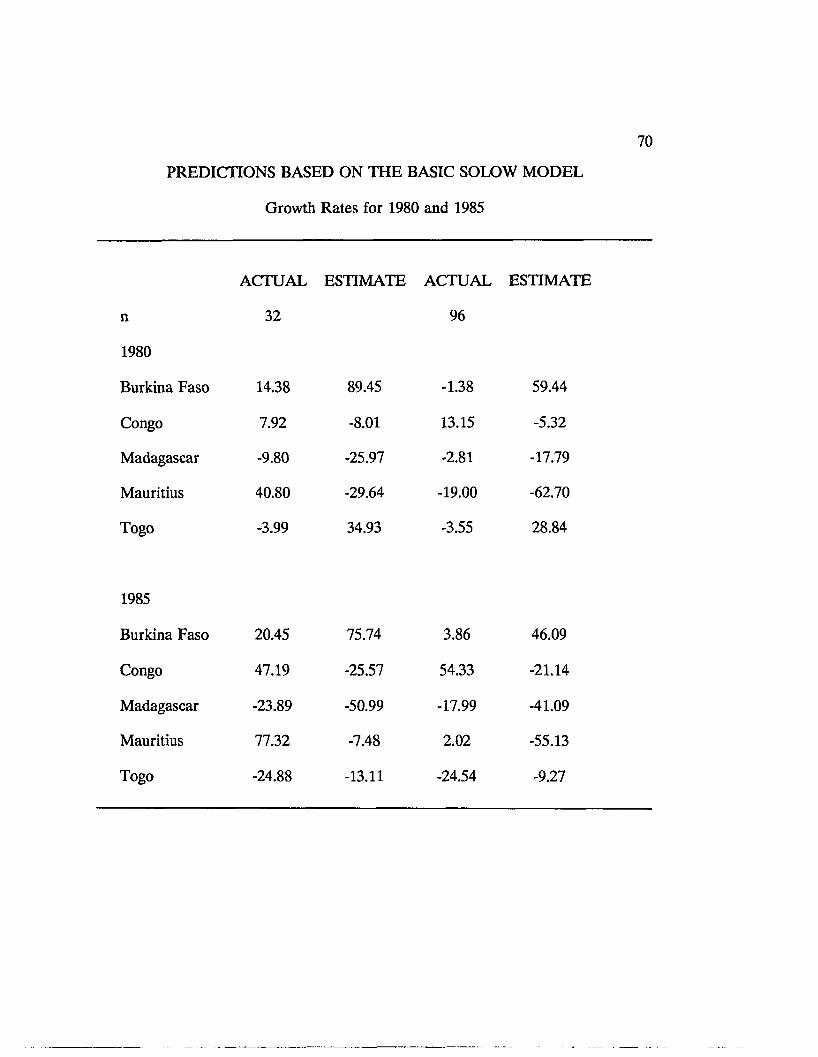
70

PREDICTIONS BASED ON THE BASIC SOLOW MODEL

Growth Rates for 1980 and 1985

ACTUAL ESTIMATE ACTUAL ESTIMATE

n 32 96

1980

Burkina Faso 14.38 89.45 -1.38 59.44

Congo 7.92 -8.01 13.15 -5.32

Madagascar -9.80 -25.97 -2.81 -17.79

Mauritius 40.80 -29.64 -19.00 -62.70

Togo -3.99 34.93 -3.55 28.84

1985

Burkina Faso 20.45 75.74 3.86 46.09

Congo 47.19 -25.57 54.33 -21.14

Madagascar -23.89 -50.99 -17.99 -41.09

Mauritius 77.32 -7.48 2.02 -55.13

Togo -24.88 -13.11 -24.54 -9.27

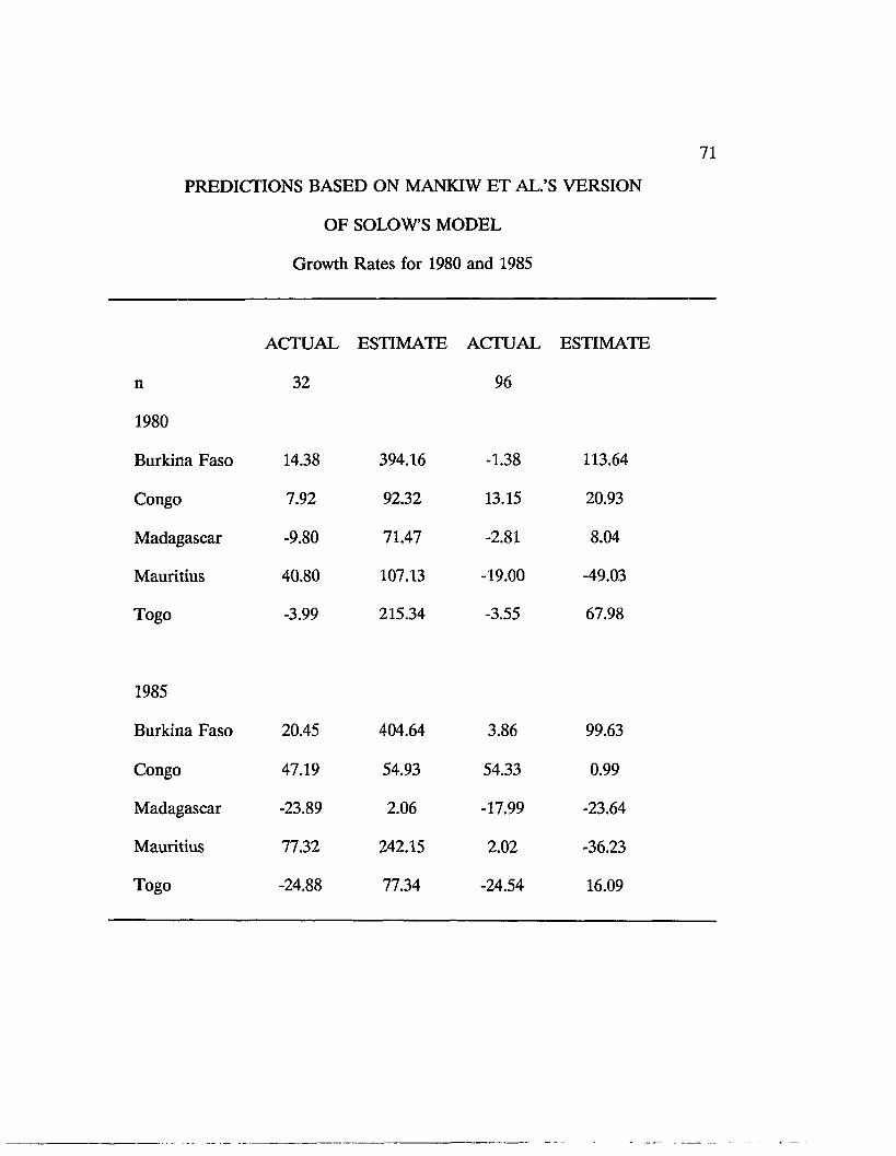
71

PREDICTIONS BASED ON MANKIW ET AL.’S VERSION

OF SOLOW’S MODEL

Growth Rates for 1980 and 1985

ACTUAL ESTIMATE ACTUAL ESTIMATE

n 32 96

1980

Burkina Faso 14.38 394.16 -1.38 113.64

Congo 7.92 92.32 13.15 20.93

Madagascar -9.80 71.47 -2.81 8.04

Mauritius 40.80 107.13 -19.00 -49.03

Togo -3.99 215.34 -3.55 67.98

1985

Burkina Faso 20.45 404.64 3.86 99.63

Congo 47.19 54.93 54.33 0.99

Madagascar -23.89 2.06 -17.99 -23.64

Mauritius 77.32 242.15 2.02 -36.23

Togo -24.88 77.34 -24.54 16.09

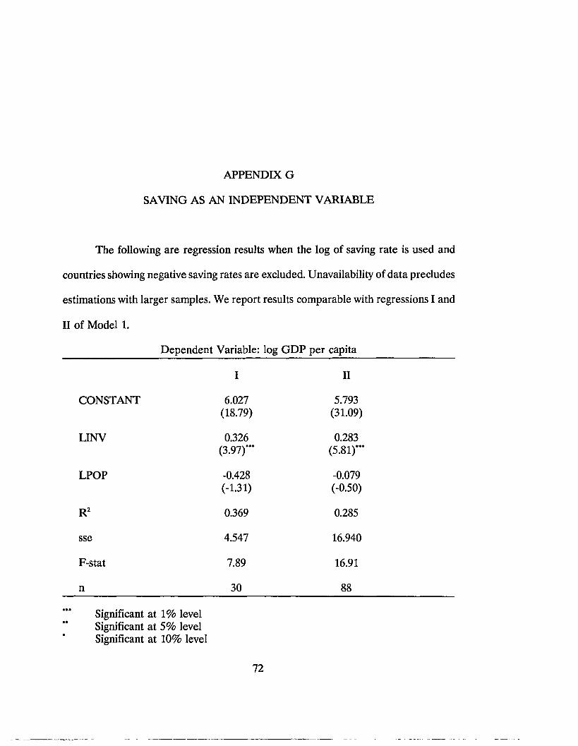
APPENDIX G

SAVING AS AN INDEPENDENT VARIABLE

The following are regression results when the log of saving rate is used and

countries showing negative saving rates are excluded. Unavailability of data precludes

estimations with larger samples. We report results comparable with regressions I and

II of Model 1.

Dependent Variable: log GDP per capita

I II

CONSTANT 6.027 5.793(18.79) (31.09)

LINV 0.326 0.283(3.97)“* (5.81)***

LPOP -0.428 -0.079(-1.31) (-0.50)

R2 0.369 0.285

sse 4.547 16.940

F-stat 7.89 16.91

n 30 88

Significant at 1% level Significant at 5% level Significant at 10% level

72

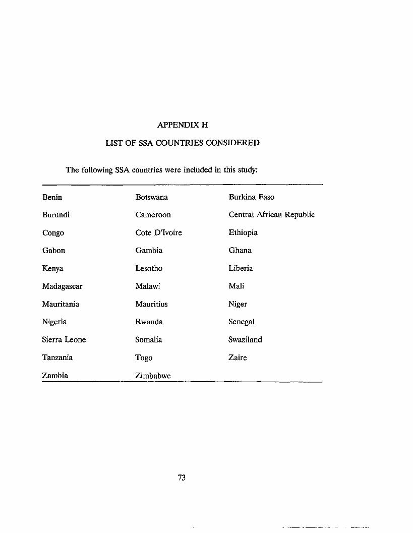
APPENDIX H

LIST OF SSA COUNTRIES CONSIDERED

The following SSA countries were included in this study:

Benin Botswana Burkina Faso

Burundi Cameroon Central African Republic

Congo Cote D’Ivoire Ethiopia

Gabon Gambia Ghana

Kenya Lesotho Liberia

Madagascar Malawi Mali

Mauritania Mauritius Niger

Nigeria Rwanda Senegal

Sierra Leone Somalia Swaziland

Tanzania Togo Zaire

Zambia Zimbabwe

73

BIBLIOGRAPHY

Aghevli, Bijan B., J. M. Boughton, P. J. Monteil, D. Villanueva, and G. Woglom. "The Role of National Saving in the World Economy." IMF Occasional Paper 67 (March 1990).

Azariadis, C., and A. Drazen. "Threshold Externalities in Economic Development." Quarterly Journal of Economics 105 (May 1990): 501-26.

Barro, R. J. "Economic Growth in a Cross Section of Countries." Quarterly Journal of Economics 102 (May 1991): 407-443.

Barro, R. J. "Human Capital and Economic Growth" in Federal Reserve of Kansas City, Policies for Long-Run Economic Growth. Kansas City: Missouri, 1992.

Barro, R. J. and X. Sala-i-Martin. "Convergence." Journal of Political Economy 100 (April 1992): 223-251.

Chiang, A. C. Fundamental Methods of Mathematical Economics. 3d ed.; Mc-Graw- Hill, 1984.

Darby M. R. "Causes of Declining Growth" in Federal Reserve of Kansas City, Policies for Long-Run Economic Growth. Kansas City: Missouri, 1992.

De Long, J. B., and L. H. Summers. "Equipment Investment and Economic Growth." Quarterly Journal of Economics 106 (May 1991): 445-502.

Fosu, A. K. "Exports and Economic Growth: The African Case." World Development 18 (June 1990): 831-835.

Grier, K. B., and G. Tullock. "An Empirical Analysis of Cross-National Economic Growth, 1951-80." Journal of Monetary Economics 24 (September 1989): 259- 276.

Grossman, G. M., and E. Helpman. "Trade, Innovation, and Growth." American Economic Review 80 (May 1990): 86-91.

74

75

Kahn, G. A. Symposium Summary in Federal Reserve of Kansas City, Policies for Long-Run Economic Growth. Kansas City: Missouri, 1992.

Kormendi, R. C., and P. G. Meguire. "Macroeconomic Determinants of Growth." Journal of Monetary Economics 16 (September 1985): 141-164.

Knight, M., N. Loayza, and D. Villanueva. "Testing the Neoclassical Theory of Economic." IMF Staff Papers 40 (September 1993): 512-541.

Lilien, D. M. MicroTSP (Version 7.0). Irvine, California: Quantitative Micro Software, 1990.

Landau, D. "Government Expenditure and Economic Growth: A Cross-Country Study." Southern Economic Journal 49 (January 1983): 783-792.

Levine, R. and D. Renelt. "A Sensitivity Analysis of Cross-Country GrowthRegressions." American Economic Review 82 (September 1992): 942-963.

Lucas, R. E. "Making a Miracle." Econometrica 61 (March 1993): 251-272.

Lucas, R. E. "On the Mechanics of Economic Development." Journal of Monetary Economics 22 (July 1988): 3-42.

Mankiw, N. G. "Commentary: The Search for Growth" in Federal Reserve of Kansas City, Policies for Long-Run Economic Growth. Kansas City: Missouri, 1992.

Mankiw, N. G., D. Romer, D. N. Weil. "A Contribution to the Empirics of Economic Growth." Quarterly Journal of Economics 107 (May 1992): 407-437.

Odedokun, M. O. "Factors Responsible for the Poor Economic Growth Performance of Africa in 1970’s and 1980’s: A Cross-Sectional Evidence from 42 Countries." African Development Review 5 (June 1993): 32-61.

Otani, I. and D. Villanueva. "Long-Term Growth in Developing Countries and Its Determinants: An Empirical Analysis." World Development 18 (June 1990): 769-783.

Pack, Howard. "Endogenous Growth Theory: Intellectual Appeal and Empirical Shortcomings." Journal of Economic Perspectives 8 (Fall 1993): 55-72.

Plosser, C. I. "The Search for Growth" in Federal Reserve of Kansas City, Policies for Long-Run Economic Growth. Kansas City: Missouri, 1992.

76

Ram, R. "Exports and Economic Growth in Developing Countries from Time-Series and Cross-Section Data." Economic Development and Cultural Change 36 (October 1987): 51-72.

Robey, B., S. O. Rutstein, and L. Morris. "The Fertility Decline in Developing Countries." Scientific American December 1993: 60-67.

Schultz, T. P. "Education Investment and Returns" in H. Chenery and T. N.Srinivasan. Eds., Handbook of Development Economics. Vol. 1. Amsterdam: Elsevier, 1988.

Singh, R. D. "State Intervention, Foreign Economic Aid, Savings and Growth in LDCs: Some Recent Evidence." Kvklos 38 (1985): 216-232.

Solow, R. M. "A Contribution to the Theory of Economic Growth." Quarterly Journal of Economics 29 (1956): 65-94.

Summers, R. and A. Heston. "A New Set of International Comparisons of RealProduct and Prices: Estimates for 130 Countries, 1950-1985." Review of Income and Wealth 34 (March 1988).

UNESCO, Statistical Yearbook 1963 to 1992.

Wheeler, D. "Sources of Stagnation in Sub-Saharan Africa." World Development 12 (January 1984): 1-23.

World Bank. Sub-Saharan Africa-From Crisis to Sustainable Growth. Washington, D.C.: World Bank, 1989.

World Bank. World Development Report 1989. New York: Oxford University Press, 1989.

World Bank. "Lesotho: A Development Challenge" World Bank Country Economic Report. October 1975.