Aerodynamics of a Mercedes-Benz CLK MER 331: Fluid Mechanics Written By: Zacarie Hertel Lab Partners: Evan States, Eric Robinson 2/19/2013

“I affirm that I have carried out

my academic endeavors with full

academic honesty.”

Signed: Zacarie Hertel, Evan

States, and Eric Robinson

Hertel 1

To: Professor Anderson-Lab Instructor

From: Zacarie Hertel-Student

Lab Partners: Eric Robinson, Evan States

Date: 19 February, 2013

Subject: Pressure coefficients of the Mercedes CLK model RC Car

The purpose of this memo is to show the results of the aerodynamics of a model car, a

Mercedes-Benz CLK. A 1/12 scale model of the car was placed in the wind tunnel, and pressure

measurements over the length of the car were taken at two separate velocities. From this data, it

was possible to find the pressure coefficient at each location, which varied from values between

1.52±0.15 and 0.099±0.003, with the maximum value occurring at the flat surface at the car’s

grill, and the minimum value occurring at the beginning of the roof’s flat surface. The increase in

velocity showed little to no change in the pressure coefficient at each location; however it is

recommended that more tests be run at different velocity values to get more accurate and

conclusive results.

Experiment

In this experiment, a 1/12 scale model Mercedes-Benz CLK was put into a wind tunnel.

Pressure taps were drilled into the model at key locations, so that the pressure at each point could

be measured. The locations of these taps can be found in the attachments, with the approximate

locations represented in Figure 1.The wind tunnel was set to two speeds, at a motor frequency of

20 Hz and 40 Hz, approximately 14.46±0.37 m/s and 30.98±0.49 m/s respectively. At each wind

speed, the pressure measurements were made at each location on the car in comparison to the

free stream pressure from the pitot probe using a multi-channel pressure transducer. Using this

data, it was possible to find the pressure coefficient at each location, valuable information that

can be used to scale the data to represent a full sized vehicle.

Experimental Results

The results of the experiment proved to be consistent across both of the velocities that

were used. In each case, the pressure coefficient was calculated at various points along the length

of the car. However, even with the increased speed, the coefficients remained nearly constant at

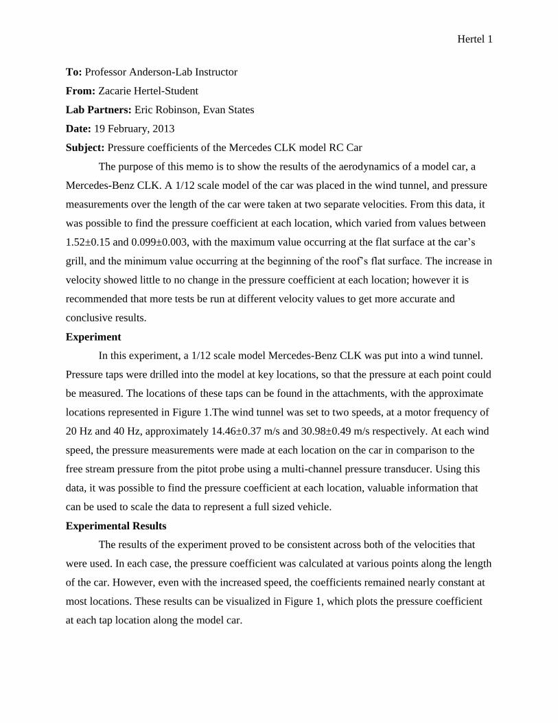
most locations. These results can be visualized in Figure 1, which plots the pressure coefficient

at each tap location along the model car.

Hertel 2

Figure 1: The pressure coefficient at the approximate location of the reading made on the model

car. Note that some uncertainty bars may not be seen due to the size of the data points.

The only points that show any major difference lie at the front of the car, which may be due to

the way the stream reacts to hitting a barrier at each speed. Since the boundary conditions are

changing with each velocity change, it is possible that it these two locations will keep changing

during further testing. More tests would be needed to see if this is the case.

Uncertainty Analysis

Overall, most of the uncertainties from the experiment seem reasonable, with the

exception of some of the data points in the 20 Hz pressure coefficient measurements. The

maximum uncertainty in velocity was 2.5% of the data, a result that is within experimental

uncertainties, and compares to known values. For the pressure coefficients, the uncertainty seems

greatly diminished in the higher velocity test. This is most likely due to the way the uncertainty

is calculated, which would be larger with lower pressure values. At the windshield base in the 20

Hz test, there is an uncertainty of over 50%. This may be due to the way the flow travels over

this portion of the car at this speed, since the pressure is nearly zero. The transducer does not

perform well near zero, so this value is expected. However, this point, as well as all others agree

with the second 40 Hz test within experimental uncertainties, so all results can be interpreted as

valid and accurate.

Recommendations

In order to accurately define the pressure coefficient at each point along the car, it is

recommended that more tests be run at different wind speed velocities. More data points would

confirm or deny the results that were found, and give a larger data set to analyze the results from.

It would also be interesting to see the change in uncertainty in the experiment, as the uncertainty

seems to drop with increased wind speed. By running more tests, a more accurate solution could

be found, and the results could then be scaled to the full sized vehicle.

Hertel 3

Attachments

Attachment 1: Sketch of the experimental set-up. Page 4

Attachment 2: Summary table for the 20 Hz data. Page 5

Attachment 3: Graphical results of the 20 Hz test. Page 6

Attachment 4: Summary table for the 40 Hz data. Page 6

Attachment 5: Graphical results of the 40 Hz test. Page 7

Attachment 6: Calculations for each of the data sets. Includes pressure, velocity, and the

pressure coefficient. Page 7

Attachment 7: The uncertainty analysis for the 20 Hz data set. Page 8

Attachment 8: The uncertainty analysis for the 40 Hz data set. Page 10

Attachment 9: Lab handout and procedure. See References[2]

References

[1] Anderson, Ann. "Measurement of Wind Tunnel Velocity." MER 331: Fluid Mechanics.

Union College, n.d. Web. 27 Feb. 2013.

<http://antipasto.union.edu/~andersoa/mer331/Lab2b_Mer331_Windtunnel.pdf>.

[2] Anderson, Ann. "Race Car Aerodynamics Project." MER 331: Fluid Mechanics. Union

College, n.d. Web. 27 Feb. 2013.

<http://antipasto.union.edu/~andersoa/mer331/Week7_Mer331_RaceCar_W13.pdf>.

Hertel 4

Attachment 1

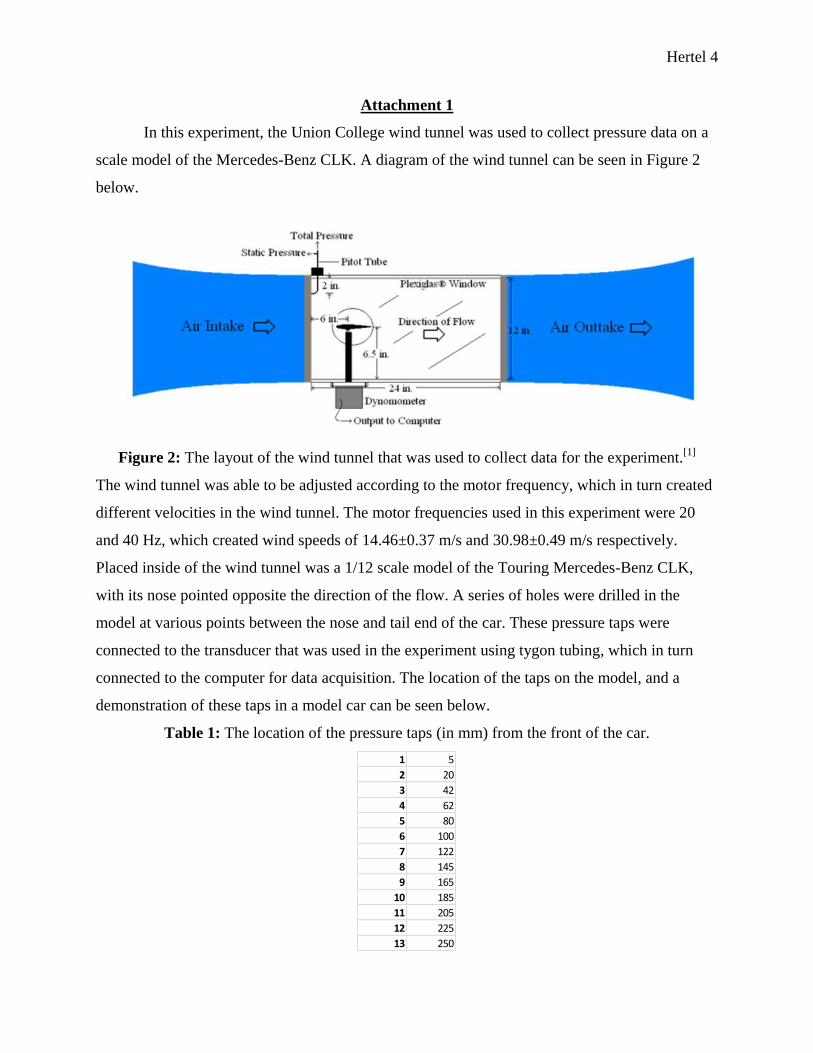
In this experiment, the Union College wind tunnel was used to collect pressure data on a

scale model of the Mercedes-Benz CLK. A diagram of the wind tunnel can be seen in Figure 2

below.

Figure 2: The layout of the wind tunnel that was used to collect data for the experiment.[1]

The wind tunnel was able to be adjusted according to the motor frequency, which in turn created

different velocities in the wind tunnel. The motor frequencies used in this experiment were 20

and 40 Hz, which created wind speeds of 14.46±0.37 m/s and 30.98±0.49 m/s respectively.

Placed inside of the wind tunnel was a 1/12 scale model of the Touring Mercedes-Benz CLK,

with its nose pointed opposite the direction of the flow. A series of holes were drilled in the

model at various points between the nose and tail end of the car. These pressure taps were

connected to the transducer that was used in the experiment using tygon tubing, which in turn

connected to the computer for data acquisition. The location of the taps on the model, and a

demonstration of these taps in a model car can be seen below.

Table 1: The location of the pressure taps (in mm) from the front of the car.

1 5

2 20

3 42

4 62

5 80

6 100

7 122

8 145

9 165

10 185

11 205

12 225

13 250

Hertel 5

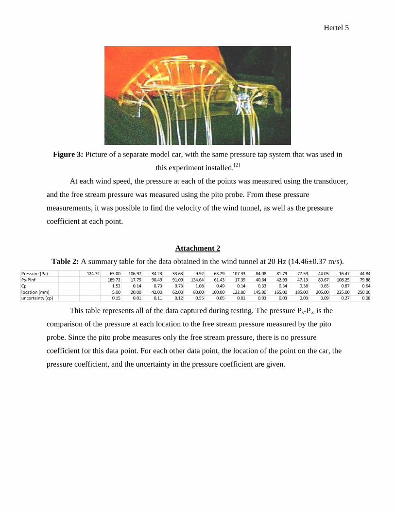
Figure 3: Picture of a separate model car, with the same pressure tap system that was used in

this experiment installed.[2]

At each wind speed, the pressure at each of the points was measured using the transducer,

and the free stream pressure was measured using the pito probe. From these pressure

measurements, it was possible to find the velocity of the wind tunnel, as well as the pressure

coefficient at each point.

Attachment 2

Table 2: A summary table for the data obtained in the wind tunnel at 20 Hz (14.46±0.37 m/s).

This table represents all of the data captured during testing. The pressure Ps-P∞ is the

comparison of the pressure at each location to the free stream pressure measured by the pito

probe. Since the pito probe measures only the free stream pressure, there is no pressure

coefficient for this data point. For each other data point, the location of the point on the car, the

pressure coefficient, and the uncertainty in the pressure coefficient are given.

Pressure (Pa) 124.72 65.00 -106.97 -34.23 -33.63 9.92 -63.29 -107.33 -84.08 -81.79 -77.59 -44.05 -16.47 -44.84

Ps-Pinf 189.72 17.75 90.49 91.09 134.64 61.43 17.39 40.64 42.93 47.13 80.67 108.25 79.88

Cp 1.52 0.14 0.73 0.73 1.08 0.49 0.14 0.33 0.34 0.38 0.65 0.87 0.64

location (mm) 5.00 20.00 42.00 62.00 80.00 100.00 122.00 145.00 165.00 185.00 205.00 225.00 250.00uncertainty (cp) 0.15 0.01 0.11 0.12 0.55 0.05 0.01 0.03 0.03 0.03 0.09 0.27 0.08

Hertel 6

Attachment 3

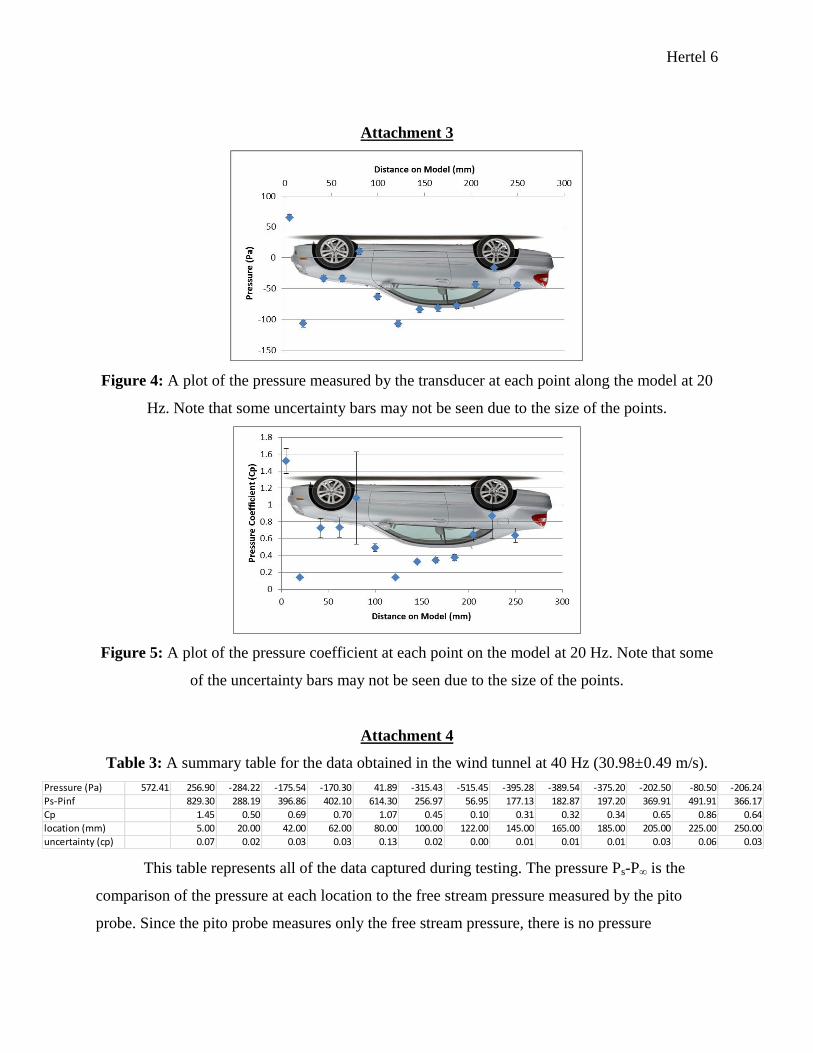
Figure 4: A plot of the pressure measured by the transducer at each point along the model at 20

Hz. Note that some uncertainty bars may not be seen due to the size of the points.

Figure 5: A plot of the pressure coefficient at each point on the model at 20 Hz. Note that some

of the uncertainty bars may not be seen due to the size of the points.

Attachment 4

Table 3: A summary table for the data obtained in the wind tunnel at 40 Hz (30.98±0.49 m/s).

This table represents all of the data captured during testing. The pressure Ps-P∞ is the

comparison of the pressure at each location to the free stream pressure measured by the pito

probe. Since the pito probe measures only the free stream pressure, there is no pressure

Pressure (Pa) 572.41 256.90 -284.22 -175.54 -170.30 41.89 -315.43 -515.45 -395.28 -389.54 -375.20 -202.50 -80.50 -206.24

Ps-Pinf 829.30 288.19 396.86 402.10 614.30 256.97 56.95 177.13 182.87 197.20 369.91 491.91 366.17

Cp 1.45 0.50 0.69 0.70 1.07 0.45 0.10 0.31 0.32 0.34 0.65 0.86 0.64

location (mm) 5.00 20.00 42.00 62.00 80.00 100.00 122.00 145.00 165.00 185.00 205.00 225.00 250.00

uncertainty (cp) 0.07 0.02 0.03 0.03 0.13 0.02 0.00 0.01 0.01 0.01 0.03 0.06 0.03

Hertel 7

coefficient for this data point. For each other data point, the location of the point on the car, the

pressure coefficient, and the uncertainty in the pressure coefficient are given.

Attachment 5

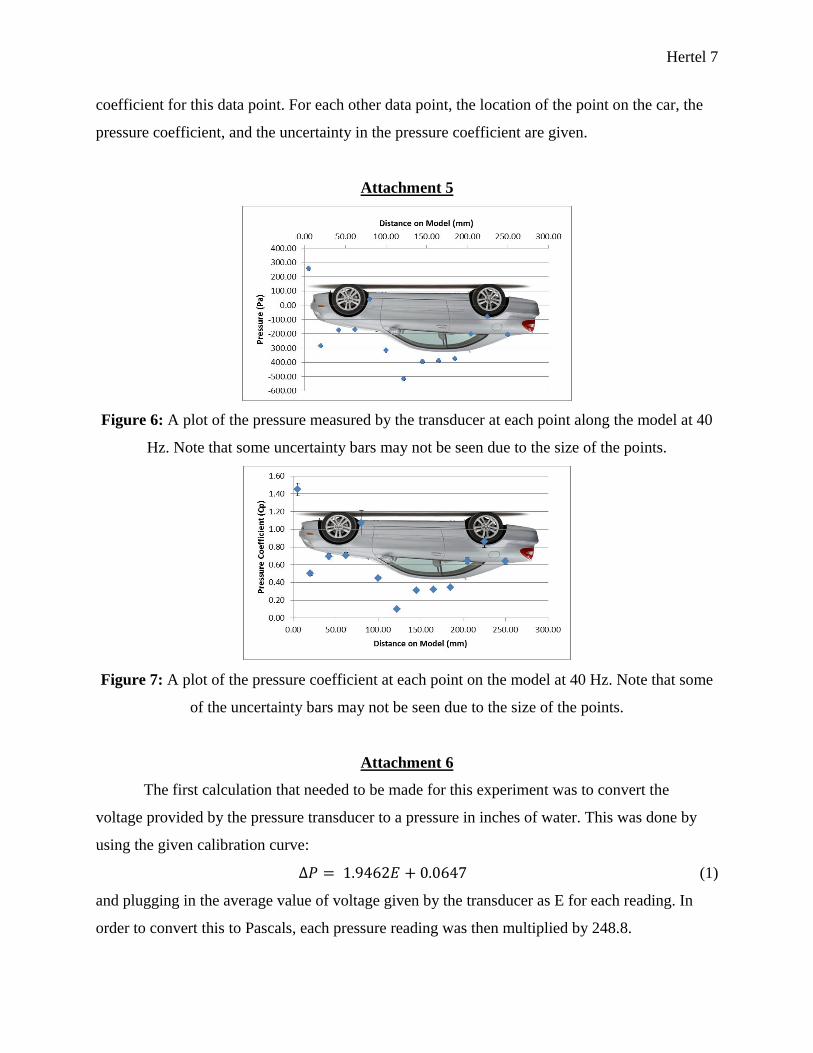
Figure 6: A plot of the pressure measured by the transducer at each point along the model at 40

Hz. Note that some uncertainty bars may not be seen due to the size of the points.

Figure 7: A plot of the pressure coefficient at each point on the model at 40 Hz. Note that some

of the uncertainty bars may not be seen due to the size of the points.

Attachment 6

The first calculation that needed to be made for this experiment was to convert the

voltage provided by the pressure transducer to a pressure in inches of water. This was done by

using the given calibration curve:

(1)

and plugging in the average value of voltage given by the transducer as E for each reading. In

order to convert this to Pascals, each pressure reading was then multiplied by 248.8.

Hertel 8

The next step of the data analysis was to find the wind speed inside the wind tunnel at

each of the motor frequencies. However, in order to do this, the density of the air needed to be

found. In order to do this, the ideal gas equation was rewritten such that:

(2)

The temperature in the room was found by reading a thermometer attached to the wind tunnel, R

is the gas constant, and P is the atmospheric pressure of 101.3 kPa. Knowing this, it was found

that the density of the air in the wind tunnel was 1.192 kg/m3. Now, this value can be used in the

velocity equation:

√

(3)

where ΔP is the free stream pressure from the pito probe.

Finally, now that the velocity of the air in the wind tunnel is known, the pressure

coefficient of each point can be found. First, the pressure (ΔP) at each location needs to be

converted to Ps-P∞, by adding the free stream pressure found by the pito probe to each value.

This allows the use of the equation:

(4)

where V is the velocity of the air in the wind tunnel, ρ is the air’s density, and Ps - P∞ is the

pressure relative to the free stream pressure.

Attachment 7

For the pressure calculation, there is not only an uncertainty given with the calibration

curve, but there is also some uncertainty due to the fluctuation in the measured data. In order to

account for both of these uncertainty sources, the equation:

√ (5)

must be used. This accounts for the deviation of the sample, which is multiplied by two to cover

a 95% confidence interval, and the uncertainty in the calibration curve of 0.02. In reality, there

may be some uncertainty in the transducer; however, it is small enough in magnitude in

comparison to the other uncertainties to be considered negligible. The standard deviation

changes in each measured value, so each data point will have an individual uncertainty, as seen

in the table below.

Hertel 9

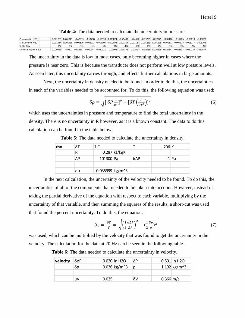
Table 4: The data needed to calculate the uncertainty in pressure.

The uncertainty in the data is low in most cases, only becoming higher in cases where the

pressure is near zero. This is because the transducer does not perform well at low pressure levels.

As seen later, this uncertainty carries through, and effects further calculations in large amounts.

Next, the uncertainty in density needed to be found. In order to do this, the uncertainties

in each of the variables needed to be accounted for. To do this, the following equation was used:

√

(

) (6)

which uses the uncertainties in pressure and temperature to find the total uncertainty in the

density. There is no uncertainty in R however, as it is a known constant. The data to do this

calculation can be found in the table below.

Table 5: The data needed to calculate the uncertainty in density.

In the next calculation, the uncertainty of the velocity needed to be found. To do this, the

uncertainties of all of the components that needed to be taken into account. However, instead of

taking the partial derivative of the equation with respect to each variable, multiplying by the

uncertainty of that variable, and then summing the squares of the results, a short-cut was used

that found the percent uncertainty. To do this, the equation:

√(

)

(7)

was used, which can be multiplied by the velocity that was found to get the uncertainty in the

velocity. The calculation for the data at 20 Hz can be seen in the following table.

Table 6: The data needed to calculate the uncertainty in velocity.

Pressure (in H2O) 0.501289 0.261249 -0.42993 -0.13758 -0.13518 0.039874 -0.25437 -0.4314 -0.33795 -0.32875 -0.31186 -0.17705 -0.06619 -0.18022

Std Dev P(in H2O) 0.001814 0.001416 0.005876 0.001213 0.001103 0.000898 0.001314 0.001184 0.001269 0.001125 0.001872 0.004128 0.001077 0.003261

% Std Dev 0% 1% -1% -1% -1% 2% -1% 0% 0% 0% -1% -2% -2% -2%

Uncertainty (in H20) 0.020326 0.0202 0.023197 0.020147 0.020121 0.02008 0.020172 0.02014 0.02016 0.020126 0.020347 0.021637 0.020116 0.021037

rho δT 1 C T 296 KR 0.287 kJ/kgK

ΔP 101300 Pa δΔP 1 Pa

δρ 0.035999 kg/m^3

velocity δΔP 0.020 in H2O ΔP 0.501 in H2O

δρ 0.036 kg/m^3 ρ 1.192 kg/m^3

uV 0.025 δV 0.366 m/s

Hertel 10

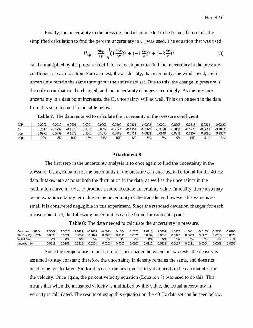
Finally, the uncertainty in the pressure coefficient needed to be found. To do this, the

simplified calculation to find the percent uncertainty in Cp was used. The equation that was used:

√

(8)

can be multiplied by the pressure coefficient at each point to find the uncertainty in the pressure

coefficient at each location. For each test, the air density, its uncertainty, the wind speed, and its

uncertainty remain the same throughout the entire data set. Due to this, the change in pressure is

the only error that can be changed, and the uncertainty changes accordingly. As the pressure

uncertainty in a data point increases, the Cp uncertainty will as well. This can be seen in the data

from this step, located in the table below.

Table 7: The data required to calculate the uncertainty in the pressure coefficient.

Attachment 8

The first step in the uncertainty analysis is to once again to find the uncertainty in the

pressure. Using Equation 5, the uncertainty in the pressure can once again be found for the 40 Hz

data. It takes into account both the fluctuation in the data, as well as the uncertainty in the

calibration curve in order to produce a more accurate uncertainty value. In reality, there also may

be an extra uncertainty term due to the uncertainty of the transducer, however this value is so

small it is considered negligible in this experiment. Since the standard deviation changes for each

measurement set, the following uncertainties can be found for each data point:

Table 8: The data needed to calculate the uncertainty in pressure.

Since the temperature in the room does not change between the two tests, the density is

assumed to stay constant; therefore the uncertainty in density remains the same, and does not

need to be recalculated. So, for this case, the next uncertainty that needs to be calculated is for

the velocity. Once again, the percent velocity equation (Equation 7) was used to do this. This

means that when the measured velocity is multiplied by this value, the actual uncertainty in

velocity is calculated. The results of using this equation on the 40 Hz data set can be seen below.

δΔP 0.0202 0.0232 0.0201 0.0201 0.0201 0.0202 0.0201 0.0202 0.0201 0.0203 0.0216 0.0201 0.0210

ΔP 0.2612 -0.4299 -0.1376 -0.1352 0.0399 -0.2544 -0.4314 -0.3379 -0.3288 -0.3119 -0.1770 -0.0662 -0.1802uCp 0.0972 0.0799 0.1578 0.1601 0.5070 0.0988 0.0751 0.0838 0.0849 0.0879 0.1357 0.3096 0.1307

uCp 10% 8% 16% 16% 51% 10% 8% 8% 8% 9% 14% 31% 13%

Pressure (in H2O) 2.3007 1.0325 -1.1424 -0.7056 -0.6845 0.1684 -1.2678 -2.0718 -1.5887 -1.5657 -1.5081 -0.8139 -0.3235 -0.8289Std Dev P(in H2O) 0.0036 0.0024 0.0035 0.0020 0.0022 0.0015 0.0026 0.0032 0.0036 0.0042 0.0033 0.0021 0.0018 0.0075

% Std Dev 0% 0% 0% 0% 0% 1% 0% 0% 0% 0% 0% 0% -1% -1%

uncertainty 0.0213 0.0206 0.0212 0.0204 0.0205 0.0202 0.0207 0.0210 0.0213 0.0217 0.0211 0.0204 0.0203 0.0250

Hertel 11

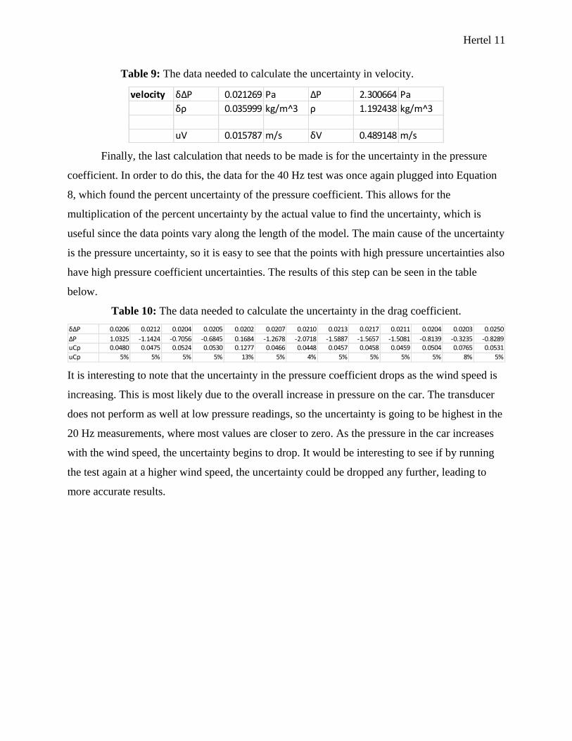
Table 9: The data needed to calculate the uncertainty in velocity.

Finally, the last calculation that needs to be made is for the uncertainty in the pressure

coefficient. In order to do this, the data for the 40 Hz test was once again plugged into Equation

8, which found the percent uncertainty of the pressure coefficient. This allows for the

multiplication of the percent uncertainty by the actual value to find the uncertainty, which is

useful since the data points vary along the length of the model. The main cause of the uncertainty

is the pressure uncertainty, so it is easy to see that the points with high pressure uncertainties also

have high pressure coefficient uncertainties. The results of this step can be seen in the table

below.

Table 10: The data needed to calculate the uncertainty in the drag coefficient.

It is interesting to note that the uncertainty in the pressure coefficient drops as the wind speed is

increasing. This is most likely due to the overall increase in pressure on the car. The transducer

does not perform as well at low pressure readings, so the uncertainty is going to be highest in the

20 Hz measurements, where most values are closer to zero. As the pressure in the car increases

with the wind speed, the uncertainty begins to drop. It would be interesting to see if by running

the test again at a higher wind speed, the uncertainty could be dropped any further, leading to

more accurate results.

velocity δΔP 0.021269 Pa ΔP 2.300664 Pa

δρ 0.035999 kg/m^3 ρ 1.192438 kg/m^3

uV 0.015787 m/s δV 0.489148 m/s

δΔP 0.0206 0.0212 0.0204 0.0205 0.0202 0.0207 0.0210 0.0213 0.0217 0.0211 0.0204 0.0203 0.0250

ΔP 1.0325 -1.1424 -0.7056 -0.6845 0.1684 -1.2678 -2.0718 -1.5887 -1.5657 -1.5081 -0.8139 -0.3235 -0.8289uCp 0.0480 0.0475 0.0524 0.0530 0.1277 0.0466 0.0448 0.0457 0.0458 0.0459 0.0504 0.0765 0.0531

uCp 5% 5% 5% 5% 13% 5% 4% 5% 5% 5% 5% 8% 5%