by Thomas W. Hertel and Marinos E. Tsigas I. … Models_Marco/Hertel and Tsigas (1997) Structure of...by Thomas W. Hertel and Marinos E. Tsigas ∗This is a draft of Chapter 2: "Structure

Structure of GTAP∗∗∗∗

by Thomas W. Hertel and Marinos E. Tsigas

∗ This is a draft of Chapter 2: "Structure of GTAP," published in T.W. Hertel (ed.), Global Trade Analysis:Modeling and Applications, Cambridge University Press, 1997.

I. INTRODUCTION AND OVERVIEW

The purpose of this chapter is to develop the basic notation, equations, and intuition behindthe GTAP model of global trade. The computer program documenting the basic model,GTAP94.TAB, is available in electronic form via the Internet (see Chapter 6). It provides completedocumentation of the theory behind the model, and when converted to executable files using theGEMPACK software suite (Harrison and Pearson, 1994), it forms the basis for implementing theapplications outlined in Part III of this book.

The organization of this chapter is as follows. We begin with an overview of the GlobalTrade Analysis Project (GTAP) model. Next, we develop the basic accounting relationshipsunderpinning the data base and model. This involves tracking value flows through the global database, from production and sales to intermediate and final demands. Careful attention is paid to theprices at which each of these flows is evaluated, and the presence of distortions (in the form oftaxes and subsidies). The relationship between these accounting relationships and equilibriumconditions in the model is then developed. This leads naturally into a discussion of the implicationsof alternative "partial equilibrium" closures whereby these equations are selectively omitted and theassociated complementary variables are fixed. The chapter then turns to the linearizedrepresentation of these accounting relations. This is the form in which they are implemented inGEMPACK, which solves the nonlinear equilibrium problem via successive updates andrelinearizations.

Section VI of this documentation turns its attention to the equations underpinning economicbehavior in the model. We deal in turn with production, consumption, global savings, andinvestment. There is also a special discussion of macroeconomic closure in the GTAP model. Thismaterial is reinforced in the closing section of the chapter by means of a numerical example using athree-region, three-commodity aggregation, in which there is a shock to a single bilateral protectionrate.

II. OVERVIEW OF THE MODEL 1

Closed Economy Without Taxes

Figure 2.1 offers an overview of economic activity in a simplified version of the GTAPmodel [see Brockmeier (1996) for a more comprehensive, graphical overview]. In this first figure,there is only one region, so there is no trade. There is also no depreciation, and no taxes or subsidiesare present. At the top of this figure is the regional household. Expenditures by this household are

10

governed by an aggregate utility function that allocates expenditure across three broad categories:private, government, and savings expenditures.2 The model user has some discretion over theallocation of expenditures across these types of final demand. In the standard closure, the regionalhousehold's Cobb��

category. However, real government purchases and savings can also be dictated exogenously (i.e.,fixed or shocked), in which case private household expenditure will adjust to satisfy the regionalhousehold's budget constraint.

This formulation for regional expenditure has some distinct advantages, as well as somedisadvantages. Perhaps the most significant drawback is the failure to link government expendituresto tax revenues. Cutting taxes by no means implies a reduction in government expenditures in theGTAP model. Indeed, to the extent that these tax cuts lead to a reduction in excess burden, regionalreal income will increase and real government expenditure will likely also rise. This lack of fiscalintegrity is dictated by the fact that the GTAP data have incomplete coverage of regional taxinstruments. Therefore the model cannot accurately predict what will happen to total tax revenue,and the user who is interested in focusing on government expenditure effects would be required tomake some exogenous assumptions in any case.

The greatest advantage of the formulation of regional expenditure displayed in Figure 2.1 isthe unambiguous indicator of welfare offered by the regional utility function. A particularsimulation might lead to lower relative prices for savings and the composite of governmentpurchases, and higher prices for the private household's commodity bundle. If real private purchasesfall, while savings and government consumption rise, is the regional household better off? Withouta regional utility function we cannot answer this question.

An alternative approach to this problem of welfare measurement involves fixing the levelof real savings and government purchases, and focusing solely on private household consumption asan indicator of welfare. However, private consumption is only slightly more than 50% of finaldemand in some regions. Forcing all the adjustment in the regional economy's final demand intoprivate consumption seems rather extreme. We believe that the assumption of fixed expenditureshares dictated by the Cobb��

That is, a rise in income implies an increase in savings and government expenditures, as well asprivate consumption.

Since Figure 2.1 assumes the absence of taxes, the only source of income for regionalhouseholds is from the "sale" of endowment commodities to firms. This income flow is representedby VOA (endw) which denotes Value of Output at Agents' prices of endowment commodities. (Acomplete glossary of GTAP notation is provided at the end of this book.) Firms combine theseendowment commodities with intermediate goods (VDFA = Value of Domestic purchases by Firmsat Agents' prices) in order to produce goods for final demand. This involves sales to privatehouseholds (VDPA = Value of Domestic purchases by Private households at Agents' prices),government households (VDGA = Value of Domestic purchases by Government household atAgents, prices), and the sale of investment goods to satisfy the regional household's demand forsavings (REGINV). This completes the circular flow of income, expenditure, and production in aclosed economy without taxes.

11

Open Economy Without Taxes

Figure 2.2 [also taken from Brockmeier (1996)] introduces international trade by addinganother region, Rest of the World (ROW), at the bottom of the figure. This region is identical instructure to the domestic economy, but details are suppressed in Figure 2.2. It is the source ofimports into the regional economy, as well as the destination for exports (VXMD = Value ofeXports at Market prices by Destination). It is important to note that imports are traced to specificagents in the domestic economy, resulting in distinct import payments to ROW from privatehouseholds (VIPA), government households (VIGA), and firms (VIFA). This innovation departsfrom most models of global trade, and was adopted from the SALTER model (Jomini et al. 1991). Itis especially important for the analysis of trade policy in regions where import intensities for thesame commodity vary widely across uses.

In moving from a closed to an open economy, we also require the introduction of twoglobal sectors, one of which is displayed in Figure 2.2. The global bank, shown in the center of thisfigure, intermediates between global savings and regional investment. As will be discussed in moredetail below, it assembles a portfolio of regional investment goods, and sells shares in this portfolioto regional households in order to satisfy their demand for savings.

The second global sector (not shown in Figure 2.2) accounts for international trade andtransport activity. It assembles regional exports of trade, transport, and insurance services andproduces a composite good used to move merchandise trade among regions. The value of theseservices precisely exhausts the differences between global fob exports, and global imports,evaluated on a cif basis.

III. ACCOUNTING RELATIONSHIPS IN THE "LEVELS"

Distribution of Sales to Regional Markets

The basic accounting relationships in the data base/model are best understood in thecontext of a flow chart. For example, Table 2.1 portrays the sources of sectoral receipts in theglobal data base. (In the data and the model all sectors produce a single output. Thus there is a one-to-one relationship between producing sectors and commodities.) At the top of the figure, VOA(i,r)refers to the Value of Output at Agents' Prices. (The general explanation for this choice of notationis as follows: value/type of transaction/type of price. See the appendix to this chapter for anexhaustive listing of variables used in the model and their description.) VOA(i,r) represents thepayments received by the firms in industry i of region r. As we will see, these payments must beprecisely exhausted on costs, under the zero pure profits assumption. The terms PS(i,r) and QO(i,r)to the right of VOA represent the price and quantity indices that make up VOA. They will bediscussed in more detail below.

If one adds back the producer tax (or deducts the subsidy) denoted by PTAX(i,r), then wearrive at the Value of Output at Market prices, VOM(i,r). This may be seen to be the sum of theValue of Domestic sales at Market prices, VDM(i,r) and the exports to all destinations, denoted asValue of eXports of i from r evaluated at domestic Market prices (in r), and Destined for s,VXMD(i,r,s). In addition, we must take account of possible sales to the international transportsector, denoted VST(i,r). These sales are designed to cover the international transport margins. They

12

are evaluated at market prices and face no further (border) taxes. Similarly, since domestic sales donot cross a border, they do not face such taxes either.

In order to convert exports to fob values, it is necessary to add the export tax, denotedXTAX(i,r,s). Note that these taxes are written in a form that is destination��

destination/source-specific trade policy measures at the level of disaggregated regions andcommodities (this varies by type of policy intervention), once the data base has been aggregatedover either commodities or regions, bilateral rates of taxation will vary due to compositionaldifferences. Therefore, it is important to maintain this bilateral detail in the modeling framework.Once the export taxes are added in, we obtain the Value of eXports at World prices by Destination,VXWD(i,r,s). The difference between this and the cif-based Value of Imports at World prices bySource, VIWS(i,r,s), is the international transportation margin: VTWR(i,r,s) refers to the Value ofTransportation at World prices by Route for commodity i, shipped from r to s.

At this point we have taken commodity i from its sector of origin in region r to its exportdestination in region s. In order to evaluate these sales at internal domestic prices in s, it isnecessary to add import taxes, MTAX(i,r,s) to get VIMS(i,r,s), the Value of Imports at Market pricesby Source. These imports from alternative sources may then be combined into a single composite,VIM(i,s), the Value of Imports of i into s at Market prices. Just as sales in the rth market had to bedistributed across various destinations, so composite imports of i into s must be distributed acrosssectors and households in the sth market. Possible uses of imports include: VIPM(i,s) � �� Valueof Imports by Private households, evaluated at Market prices: VIGM(i,s) � �� Value of Imports bythe Government, evaluated at Market prices; and VIFM(i,j,s) � �� Value of Imports by Firms inindustry j, at Market price. In a similar fashion, domestic sales, denoted VDM(i,r), must bedistributed across private household, government, and firms' uses, as shown at the bottom of Table2.1.

Sources of Household Purchases

Having distributed sales across various markets and taken full account of intervening taxesand transport margins, we are now in a position to consider household and firms' purchases withineach of these individual markets. Table 2.2 outlines the distribution of household purchases oftradeable commodities. The top half of this figure pertains to private household purchases, denotedVPA(i,s), to represent the Value of Private household purchases at Agents' prices. This representsthe sum of expenditures on domestically produced goods, VDPA(i,s), and composite imports,evaluated at agents' prices, VIPA(i,s). Once private household commodity taxes, IPTAX(i,s), arededucted, this brings us to the Value of Imports by the Private household at Market prices,VIPM(i,s), which is the point where we left Table 2.1. Similarly, deducting domestic commoditytaxes, DPTAX(i,s), from VDPA(i,s) yields VDPM(i,s), the Value of Domestic purchases by thePrivate household, at Market prices. Thus we have completed the link between industry sales atagents' prices (top of Table 2.1) and private household purchases at agents' prices (top of Table 2.2).The bottom half of Table 2.2 is completely analogous, only P is replaced by G in order to representpurchases by the government household.

13

Sources of Firms' Purchases and Household Factor Income

Next, turn to firms' purchases of intermediate and primary factors of production. The top ofTable 2.3 tackles the intermediate inputs, starting with the Value of Firms' purchases of i, by sectorj, in region s at Agents' prices, VFA(i,j,s). This may be broken into the domestic and importedcomponents, VDFA(i,j,s) and VIFA(i,j,s). Deducting intermediate input taxes, DFTAX(i,j,s) andIFTAX(i,j,s), reduces these values to market prices, VDFM(i,j,s) and VIFM(i,j,s), which are thesame as the values reported at the bottom of Table 2.1.

Firms also purchase services of nontradeable commodities, which in this model are termedendowment commodities. (In the current data base, these include: agricultural land, labor, andcapital.) The next part of Table 2.3 traces the value flows from the firms employing these factors ofproduction, back to the households supplying them. Note that by deducting taxes on endowment iused in industry j, ETAX(i,j,s), we can move from the Value of Firms' purchases at Agents' prices,VFA(i,j,s), to the Value of Firms' purchases at Market prices, VFM(i,j,s). The final section of Table2.3 makes the link between firms' receipts [i.e., VOA(j,s)], as developed in Table 2.1, and firms'expenditures [i.e., VFA(i,j,s)], as shown in Table 2.3. Zero pure economic profits means thatrevenues must be exhausted on expenditures, once accounting for all tradeable (i.e., intermediate)inputs and endowment (i.e., primary) factors of production.

Table 2.4 details the sources of household factor income. Here, it is necessary todistinguish between endowment commodities that are perfectly mobile, and therefore earn the samemarket return (ENDWM_COMM), and those that are sluggish to adjust and that therefore sustaindifferential returns in equilibrium (ENDWS_COMM). In the former case, we may simply sum overall usage of the factor � ��

supply of primary factor i in region s, HTAX(i,s), in order to obtain the Value of this endowment's"Output" at Agents' prices (VOA). The latter is the amount actually received by the privatehousehold supplying the factor in question.

In the case of the sluggish endowment commodities (e.g., land), shocks to the model willintroduce differential price changes across sectors. This is reflected in the presence of an industryindex (j), in the price component of VFM(i,j,s). These differential prices are then combined into acomposite return to the sluggish endowment, at market prices, via a unit revenue function. Theresulting Value of endowment Output at Market prices, VOM(i,s), is then handled in the same wayas for mobile commodities, deducting household income taxes to arrive at the VOA(i,s).

Disposition and Sources of Regional Income

When taxes are present, the computation of disposable income for the regional householdin Figures 2.1 and 2.2 becomes much more complex. At the top of Table 2.5, we have the conditionthat expenditures on private, government, and savings commodities must precisely exhaust regionalincome. This is followed by the expression that decomposes income by source. We begin by addingup endowment income (recall Figures 2.1 and 2.2). Note that all such income earned within a regionaccrues to households in that same region. From this, we must deduct depreciation expensesrequired to maintain the integrity of the initial capital stock, VDEP(r), thereupon adding net taxreceipts and rents associated with any quantitative restrictions.

Rather than keeping track of individual tax/subsidy flows in the model, the approach takenhere is to compare the value of a given transaction, evaluated at agents', market, or world prices. If

14

there is a discrepancy between what households receive for their labor supply and the value of thissupply at market prices, then the difference must equal HTAX(i,r), as shown in Table 2.4.

Alternatively, this tax revenue could be rewritten in terms of an explicit ad valorem tax rate, r)(i,τ ,by noting that the household's supply price of endowment i is given by:

,r)r)PM(i,TO(i, = r)r))PM(i,(i, - (1 = r)PS(i, τ

where TO(i,r) is referred to as the power of the ad valorem tax. Therefore:

r).QO(i, r)PM(i, r)(i, = r)QO(i, r)PM(i, r))TO(i, - (1 = r)VOA(i, - r)VOM(i, τ

Thus, the fiscal implications of all tax/subsidy programs may be captured by comparison of thevalue of a given transaction at agents' versus market (or market versus world) prices. We assumethat taxes levied in region r always accrue to households in region r.

The remaining terms in the income expression given in Table 2.5 account for all the otherpossible sources of tax revenues/subsidy expenditures in each regional economy. These include:primary factor taxes on firms, commodity taxes on households', and firms' purchases of tradeablegoods and trade taxes.3

Figures 2.3 and 2.4, taken from Brockmeier (1996), offer graphical depictions of borderinterventions in GTAP. The two panels in Figure 2.3 refer to the case of export interventions.(Because there are many export destinations, we can interpret the supply curve as representingsupply, net of sales to domestic uses and other export markets.) In the first panel, the domesticprice exceeds the world price (PM(i,r) > PFOB(i,r,s)), indicating the presence of a subsidy, so thatXTAX(i,r,s) = VXWD(i,r,s) - VXMD(i,r,s) < 0. In the second panel, the opposite case is presented.Here, the world price is above the market price and their difference contributes positively toregional income. This will be the case regardless of the source of discrepancy in VXWD and VXMD.For example, if this difference arises due to export restraints, as opposed to taxation, then theresulting income flow is due to quota rents. Nevertheless, it still accrues to the region of origin (r).

The two panels in Figure 2.4 refer to the income consequences of import interventions.Because GTAP adopts the Armington approach to import demand, differentiating products byorigin, there is no domestic supply of the imported good. Therefore the demand schedule in thesepanels is conditional on aggregate demand for commodity i in region s, as well as the prices ofcompeting imports and the domestic market price of i in region s. The excess supply schedule forimports of i from r to s depends on supply conditions in r as well as demand for this commodity inregion s.

When the market price exceeds the world price, PMS(i,r,s) > PCIF(i,r,s), then MTAX(i,r,s)> 0 and this term contributes positively to regional income. This can arise if there is a tariff onimports, or it could be due to an import quota. In the case of a binding quota on imports of i into sfrom r:

0 > s)r,QXS(i, s)r,PCIF(i, 1) - s)r,(TMS(i, =

s)r,VIWS(i, - s)r,VIMS(i,

15

represents the associated quota rents. In this instance, the closure must be modified so thatQXS(i,r,s) is exogenous and the tax equivalent, TMS(i,r,s) is endogenous. Again, these quota rentsare assumed to accrue to the region administering the quota.

Global Sectors

In order to complete the model, it is necessary to introduce two global sectors. The globaltransportation sector provides the services that account for the difference between fob and cif valuesfor a particular commodity shipped along a specific route: VTWR(i,r,s) = VIWS(i,r,s) - VXWD(i,r,s).Summing over all routes and commodities gives the total demand for international transportservices shown at the top of Table 2.6. The supply of these services is provided by individualregional economies, which export them to the global transport sector [VST(i,r)]. We do not haveinformation that would permit us to associate regional transport services exports with particularcommodities and routes. Therefore, all demand is met from the same pool of services, the price ofwhich is a blend of the price of all transport services exports.

The other required global sector is the global banking sector. This intermediates betweenglobal savings and investment, as described in Table 2.7. It creates a composite investment good(GLOBINV), based on a portfolio of net regional investment (gross investment less depreciation),and offers this to regional households in order to satisfy their savings demand. Therefore, all saversface a common price for this savings commodity (PSAVE). A consistency check on the accountingrelationships described up to this point involves separately computing the supply of the compositeinvestment good and the demand for aggregate savings. If (1) all other markets are in equilibrium,(2) all firms earn zero profits (including the global transport sector); and (3) all households are ontheir budget constraint, then global investment must equal global savings by virtue of Walras' Law.

Finally, the value of the beginning of period capital stock, VKB(r), is updated by regionalinvestment, REGINV(r), less depreciation, VDEP(r). This yields the value of ending capital stocks,VKE(r). This relationship is shown at the bottom of Table 2.7.

IV. EQUILIBRIUM CONDITIONS AND PARTIAL EQUILIBRIUM CLOSURES

Thus far, we have said nothing about the behavior of individual firms and households.Neoclassical restrictions on such behavior are not necessary to obtain full general equilibriumclosure. Rather, it is the exhaustive accounting relationships outlined above that make our modelgeneral equilibrium in nature. If any one of them is not enforced, Walras' Law will fail to hold.Since most economists are accustomed to seeing equilibrium conditions written in terms ofquantities, not values, it is useful to demonstrate that the accounting relationships provided abovedo indeed embody the customary general equilibrium relationships. Consider, for example, themarket clearing condition for tradeable commodity supplies:

. s)r, i, ( VXMD + r) i, ( VST + r)i, ( VDM = r) i, ( VOMREGs∑

ε(2.1)

16

This may be rewritten in terms of quantities and a common domestic market price for i in region r:

. s)r, i, ( QXS + r) i, ( QST + r) i, ( QDS* r) i, ( PM

= r) i, ( QO* r) i, ( PM

REGs

∑

ε

(2.2)

Upon dividing by PM(i,r) we obtain the usual form of the tradeable commodity market clearingcondition:

. s)r, i, ( QXS + r) (i, QST + ) ri, ( QDS = r) i, ( QOREGs∑

ε(2.3)

A similar exercise may be applied to the market clearing conditions for nontradeable commodities.In sum, any market clearing condition can be converted to value terms by multiplying by a commonprice. In so doing, we circumvent the need to partition value flows into prices and quantities. Thishas the added benefit of vastly simplifying the problem of model calibration, as we will see below.

Having verified that the accounting relationships embody all the necessary generalequilibrium conditions, we turn to the problem of creating special closures in which some of theseconditions are dropped. This, in turn, permits one to fix certain variables exogenously, as is doneimplicitly in partial equilibrium analysis. The problem lies in ascertaining which variables areassociated with which equilibrium conditions. This is akin to identifying the complementaryslackness conditions associated with the general equilibrium model.

Perhaps the most obvious complementarity is that between prices and market clearingconditions. Clearly if the latter are to hold, prices must be free to adjust to resolve any imbalancebetween supply and demand. Therefore, if we fix the price of a tradeable commodity, we musteliminate the associated market clearing condition, equation (2.3). A common partial equilibriumclosure for the analysis of farm and food issues involves fixing the prices of all nonfoodcommodities. In order to implement this closure in our model, all nonfood market clearingconditions must be dropped. (The "dropping" of individual equations is achieved by endogenizingslack variables in the equations to be eliminated. We must always retain equal numbers ofendogenous variables and equations if the model is to provide a unique equilibrium solution.)

It is also common in partial equilibrium analyses to assume that the opportunity cost ofnonspecific factors is exogenous. For example, in the case of agriculture, one might assume that thelabor wage and capital rental rates are fixed. If this is to be done, then the associated regionalmarket clearing conditions for these nontradeable primary factors must be dropped. Similarly,income may be fixed, provided the income computation equation is eliminated.

But what about quantities? Should any of them be fixed? Having fixed the price ofnonfood commodities, for example, it hardly makes sense to permit their supplies to be determinedendogenously. Any sector experiencing a rise in costs would be driven out of business altogetherunder such circumstances. For this reason it makes sense to fix nonfood output levels and drop theassociated zero profit conditions. These partial equilibrium assumptions, for the example of a foodpolicy shock, may be summarized as follows:� Nonfood output levels and prices are exogenous.� Income is exogenous.� Nonspecific primary factor rental rates are exogenous.

17

V. LINEARIZED REPRESENTATION OF ACCOUNTING EQUATIONS

Solution via a Linearized Representation: While the accounting relationships detailed inFigures 2.1 and 2.2 and Tables 2.1��

attractive to write the behavioral component of the model in terms of percentage changes in pricesand quantities.4 Indeed, we are usually most interested in these percentage changes, as opposed totheir levels values. Expressing this nonlinear model in percentage changes does not precludesolution of the true nonlinear problem. Solution of nonlinear AGE models via a linearizedrepresentation (Pearson 1991)5 involves successively updating the value-based coefficients via theformula:

q, + p = d(PQ)/PQ = dV/V

where the lowercase p and q denote percentage changes in price and quantity.Figure 2.5 provides a graphical exposition of one method of solving a nonlinear model via

its linearized representation. For simplicity, the entire model is given by a single equation g(X,Y) =0, where X is exogenous and Y is endogenous. The initial equilibrium is represented by the point(X0, Y0). Our counterfactual experiment involves shocking the exogenous variable to X1, andcomputing the resulting endogenous outcome Y1. If we simply evaluated the linearizedrepresentation of the model at (X0, Y0) the equations would predict the outcome BJ = (X1, YJ). Thisis the Johansen approach, and it is clearly in error, since YJ >> Y1. This type of error has led tocriticism of the individuals using linearized Computable General Equilibrium (CGE) models.

However, note that the accuracy of the linearized model can be considerably enhanced bybreaking the shock to X into two parts and updating the equilibrium after the first shock. Thisapproach takes us from point A to C2 to B2. It is termed Euler's method of solution via linearizedrepresentation. By increasing the number of steps, one obtains an increasingly accurate solution ofthe nonlinear model.

Since Euler's contribution, this approach of relinearizing the model has been considerablyrefined to yield more rapid convergence to (X1, Y1). [See Harrison and Pearson (1994), section 2.5,for more details.] The default method used for solving the GTAP model is Gragg's method, withextrapolation. In this case the model is solved several times, each time with a successively finergrid. An extrapolated solution is formed based on these results. As illustrated in Harrison andPearson (1994, pp. 2�� !� ��

Form of Accounting Equations: Linearization of the accounting equations involves totaldifferentiation so they appear as a linear combination of appropriately weighted price and quantitychanges. For example, the tradeable market clearing condition [equation (2.3)] becomes:

s)r, i, ( qxs s)r, i, ( QXS +

r) i, ( qst r) i, ( QST +r)i, ( qds r)i, ( QDS = r) i, ( qo r) i, ( QO

REGs∑

ε

(2.4)

where the lowercase variables are again percentage changes. Multiplying both sides by the commonprice PM(i,r) yields equation (1) in Table 2.8. Here the coefficients are now in value terms. [It isnever necessary actually to compute price and quantity levels (P and Q) under this approach,although this can be done if one chooses to define initial units by choosing, for example, PM(i,r) =1] . Also, note that a slack variable has been introduced into this equation in Table 2.8. It is indexedover all tradeable commodities and regions. By endogenizing selected components of this variable(which appear only in this equation), we are able to eliminate selectively market clearing for

18

individual products. In this case, with the associated tradeable price fixed exogenously (pm(i,r) =0), the endogenous change in tradslack(i,r) accounts for the excess of supply over demand in thenew equilibrium (as a percentage of output in the initial equilibrium).

The next two equations in Table 2.8 enforce equilibrium in the domestic market fortradeable commodities, either that which is imported from region r in the case of equation (2) orthat which is produced domestically in the case of equation (3). Therefore, the common price isonce again a domestic market price. We do not include slack variables in these equations, since theyrefer to the same commodity treated in equation (1). To achieve a partial equilibrium closure, it issufficient to fix the price of this good at one place in the model.

Equations (4) and (5) in Table 2.8 refer to market clearing for the nontradeable, endowmentcommodities. As noted above, the model distinguishes between primary factors that are perfectlymobile across sectors, and those which are "sluggish" in their adjustment. The latter class ofendowment commodities can exhibit differential equilibrium rental rates across uses. In the case ofmobile endowments, equation (4), the presence of a common market price permits the equilibriumrelationship to be written in terms of values at domestic market prices. A slack variable isintroduced to permit us selectively to eliminate the market clearing equations and fix rental rates onthe respective endowment commodities. In the case of sluggish commodities, no such commonprice exists and sectoral demands are equated to sectoral supplies. The latter are generated from aConstant Elasticity of Transformation (CET) revenue function, which transforms one use of theendowment into another.

Equation (6) in Table 2.8 is the zero pure profit condition. Since firms are assumed tomaximize profits, the quantity changes drop out when the expression at the bottom of Table 2.3 istotally differentiated in the neighborhood of an optimum (e.g., Varian 1978 p. 267). This leaves anequation relating input prices to output prices, where these percentage changes are weighted byvalues at agent's prices. For computational convenience we use different variables to refer to firms'prices for composite intermediate inputs (pf) and endowment commodities (pfe). The presence ofprofitslack(j,r) permits us to fix output and eliminate the zero profit condition for any sector j in anyregion r. In a similar fashion, equation (7) is the zero profit condition for the international transportsector. Here, the total value of transport services (VT) is constrained to equal the total value ofservices exports to this sector/use (VST), as described in Table 2.6.

Equation (8) in Table 2.8 assures the complete disposition of regional income (recall Table2.5). This is done by first deducting savings and government spending (each of which may beexogenously specified under some closures) from disposable regional income, thereupon allocatingthe remainder to private household expenditures PRIVEXP(r). It is followed by equation (9), whichgenerates available income in each region. This is the most complicated equation in the model. Itmust take account of changes in the value of regional endowments, as well as changes in the netfiscal revenues owing to the ad valorem taxes/subsidies. Even if these tax rates do not change,revenues will change due to changes in market prices and quantities. Therefore, in differential form,each of the values must be postmultiplied by the percentage change in both the price and quantitycomponents of the value flow.

Note that in Table 2.8 the quantity change is common for each of the transactions taxes inequation (9). For example, in the case of the tax on firms' use of primary factors, the percentagechange in firms' derived demands, qfe(i,j,r ), enters both terms. This is simply a reflection of the factthat the tax refers to a particular transaction in quantities. In contrast, the prices faced by firms are:(1) potentially different from market prices, and (2) free to change at different rates when the tax

19

rate dividing them is changed. This is reflected by the fact that VFA(i,j,r ) is post-multiplied bypfe(i,j,r ), while VFM(i,j,r ) changes according to pm(i,r).

Before going through (Table 2.8) equation (9) in more detail it is useful to considerexplicitly the taxes associated with each of these price differences. These are revealed in the pricelinkage equations given in Table 2.9; for example, equation (15) shows the role of income/outputtaxes that drive a wedge between VOM(i,r) and VOA(i,r). The power of the ad valorem tax in thiscase is given by TO(i,r) = VOA(i,r)/VOM(i,r). Therefore, when TO(i,r) > 1, firms/households areactually receiving a subsidy on the commodity supplied. Similarly, if dTO(i,r)/TO(i,r) = to(i,r) > 0then the subsidy is increased. This choice of notation may seem odd, but it gives rise to a usefulpattern across tax instruments. In particular, we adopt the rule that tax rates are always defined asthe ratio of agent's prices to market prices (or market prices to world prices in the case of bordertaxes).

Turning to the next price linkage relationship, equation (16) in Table 2.9, we note that anincrease in TF(i,j,r ), that is, tf(i,j,r ) > 0, will cause an increase in tax revenues. This is because inthis case the firms in sector j of region r purchasing mobile endowment commodity i will be forcedto pay more, relative to the market price, that is, pfe(i,j,r ) > pm(i,r). Owing to the fact that there isnot a unique market price for the sluggish endowment commodities purchased by firms, we requirea separate price linkage, equation (17) in this case.

Equations (18)�"�#! �� $�� % �� &��

and agents purchasing domestically produced, tradeable commodities. These commoditytransaction taxes can potentially vary not only across commodities and regions, but also acrossfirms and households in each region. Similarly, equations (21)�"�'! �� &��

the domestic market price of imports of i, by source r, and diverse agents in region s.Equation (24) in Table 2.9 establishes the percentage change in the domestic market price

for tradeable commodity i in region s, based on the change in the border price of that product,pcif(i,r,s) as well as two types of border interventions. Both are ad valorem import tariffs. The first,tms(i,r,s), is bilateral in nature, while the second, tm(i,s), is source-generic. The latter may be usedto insulate the domestic economy from world price changes. This is done by endogenizing tm(i,s)and establishing some domestic price target. In this model, we choose to fix the ratio of thedomestic market price for i to the price of the import composite. This is conveniently defined in thenext price linkage, equation (25). In the normal closure, tm(i,s) is exogenous and pr(i,s) isendogenous. However, we imitate the European Union's variable import levy on food products bypermitting tm(i,s) to vary so as to fix pr(i,s). In this circumstance, domestic consumers have noincentive to substitute imports for domestic food.

Equation (26) (in Table 2.9) links pcif(i,r,s) and pfob(i,r,s). Its derivation is based on theassumption that revenues must cover costs on all individual routes, for all commodities. Thus thechange in the cif price is a weighted combination of the change in the fob price and the change in ageneral transport cost index, pt, where the weights refer to the shares of fob costs [FOBSHR(i,r,s)]and transport costs [TRNSHR(i,r,s)] in cif costs. To the extent that firms engage in cross-subsidization or the costs of transport services on different routes move independently, this equationwill be inaccurate. It is also important to note the implications of equation (26) for pricetransmission across markets. The greater the transport margin along a given route (i.e.,TRNSHR(i,r,s) larger), the weaker the link between a change in the price of i in the export market rand the corresponding change in destination market s.

Equation (27) completes the "circle" of price linkages in Table 2.9 by connecting pfob(i,r,s)and domestic market price, pm(i,r). As was the case on the import side, there are two types of

20

export taxes. The first, txs(i,r,s) is destination-specific, while the second, tx(i,r), is destination-generic. The latter may be "swapped" with the normally endogenous change in sectoral output, inorder to insulate domestic producers from the vagaries of world markets. For example, this variableexport tax/subsidy has been used in modeling the European Union's (EU) common agriculturalpolicy. Note that since these export taxes refer to the ratio of domestic market prices to worldprices, an increase in TXS(i,r,s) results in a fiscal outflow, that is, a subsidy on exports.

Having established the linkage between prices in this model, we are in a position to returnto the income computation equation (9) in Table 2.8. In particular, consider the effect of omittingsome component of this complicated equation, say, income taxes. How will this affect, for example,a welfare analysis of trade policy reform? Given the presence of income taxes in the initialequilibrium data base, VOM(i,r) > VOA(i,r), if the experiment in question does not alter the rate ofincome taxation, then to(i,r! ( # �� ) ( ps(i,r) = pm(i,r) ∀��. This means the two terms insquare brackets [*] change at the same rate. If this change is positive, then omission of this termwill lead to an understatement of income tax revenues and a subsequent understatement ofdisposable income and household welfare in the new equilibrium. In sum, even when distortions arenot affected by a given policy experiment it is important to acknowledge their presence in theeconomy if an accurate welfare analysis is to be provided.

The final group of accounting equations in Table 2.8 refer to global savings andinvestment. Because this is a comparative static model, current investment does not augment theproductive stock of capital available to firms. The latter is constrained by beginning-of-periodcapital stock which is exogenous. Therefore, there is only a limited role for investment in oursimulations. When investment (and savings) is specified exogenously it will facilitate accumulationof the targeted end-of-period capital stock [see equation (10)]. When investment is endogenous itadjusts in order to accommodate the global demand for savings. (More discussion of thesemacroeconomic closure issues is provided below.) Equation (11) aggregates regional grossinvestment into global net investment. Equation (13) aggregates regional savings, and equations(12) and (14) permit us either to force the two to be equal (walraslack is exogenous) or verifyWalras' Law (walraslack is endogenous and should be found equal to zero in the solution).

VI. BEHAVIORAL EQUATIONS

Firm Behavior

The "Technology Tree": Figure 2.6 provides a visual display of the assumed technology forfirms in each of the industries in the model. This kind of a production "tree" is a convenient way ofrepresenting separable, constant returns-to-scale technologies. At the bottom of the inverted tree arethe individual inputs demanded by the firm. For example, the primary factors of production are:land, labor, and capital. Their quantities are denoted QFE(i,j,s), or, in percentage change form,qfe(i,j,s). (For the time being, please ignore the terms in brackets [.] in Figure 2.6. They refer torates of technical change, to which we will turn momentarily.) Firms also purchase intermediateinputs, some of which are produced domestically, qfd(i,j,s), and some of which are imported,qfm(i,j,s). In the case of imports, the intermediate inputs must be "sourced" from particularexporters, qxs(i,r,s). Recall from Figure 2.1 that this sourcing occurs at the border, sinceinformation on the composition of imports by sector is unavailable; hence the dashed line between

21

the firms' production tree and the constant elasticity of substitution (CES) nest combining bilateralimports.

The manner in which the firm combines individual inputs to produce its output, QO(i,s),depends largely on the assumptions that we make about separability in production. For example, weassume that firms choose their optimal mix of primary factors independently of the prices ofintermediate inputs. Since the level of output is also irrelevant, owing to our assumption of constantreturns to scale, this leaves only the relative prices of land, labor, and capital as arguments in thefirms' conditional demand equations for components of value-added. By assuming this type ofseparability, we impose the restriction that the elasticity of substitution between any individualprimary factor, on the one hand, and intermediate inputs, on the other, is equal. This is what permitsus to draw the production tree, for it is this common elasticity of substitution that enters the fork inthe inverted tree at which the intermediate and primary factors of production are joined. It alsorepresents a significant reduction in the number of parameters that need to be provided in order tooperationalize the model.

Within the primary factor branch of the production tree, substitution possibilities are alsorestricted to one parameter. This CES assumption is quite general in those sectors that employ onlytwo inputs: capital and labor. However, in agriculture, where a third input, land, enters theproduction function, we are forced to assume that all pairwise elasticities of substitution are equal.This is surely not true, but we do not have enough information to calibrate a more generalspecification at this point.

In general, the behavioral parameters at each level in the production tree can be specifiedby the user of the model. However, as will be seen below when we turn to the specific form of theequations used to represent firm behavior, we impose the restriction of nonsubstitution betweencomposite intermediates and primary factors. The fact that this is a very common specification inapplied general equilibrium (AGE) models is a poor justification for incorporating it into theGTAP model. Indeed, there is evidence of significant substitutability between some intermediateinputs and primary factors. For example, during the energy price shocks of the 1970s firmsdemonstrated considerable potential for conserving fuel via the purchase of new, more energy-efficient equipment. Similarly, farmers have shown considerable potential for altering the rate ofchemical fertilizer applications in response to changes in the relative price of fertilizer to land.However, these substitution possibilities are not characteristic of all intermediate inputs, and theirproper treatment requires a more flexible production function than that portrayed in Figure 2.6.6

Turning to the intermediate input side of the production tree in Figure 2.6, it can be seenthat the separability is symmetric, that is, the mix of intermediate inputs is also independent of theprices of primary factors. Furthermore, imported intermediates are assumed to be separable fromdomestically produced intermediate inputs. That is, firms first decide on the sourcing of theirimports; then, based on the resulting composite import price, they determine the optimal mix ofimported and domestic goods. This specification was first proposed by Paul Armington in 1969 andhas since become known as the "Armington approach" to modeling import demand. However, it hasbeen widely criticized in the literature. For example, Winters (1984), and Alston et al. (1990) arguethat the functional form is too restrictive and that the nonhomothetic, AIDS specification ispreferable. Although we agree that more flexible functional forms are preferable, this critique couldapply just as well to every other behavioral relationship in the model. The question is: can it beestimated/calibrated and operationalized in the context of a disaggregated global model? At thispoint the answer is "no," although progress has been made in the context of one-region models (e.g.,Robinson et al. 1993).

22

A more fundamental critique of the Armington approach is provided by the literature onindustrial organization, imperfect competition, and trade. Here, product differentiation isendogenous and it is associated with individual firms' attempts to carve out a market niche forthemselves. Early work along these lines is offered by Spence (1976), and Dixit and Stiglitz (1979).It is now the preferred approach for introducing imperfect competition into AGE models (e.g.,Brown and Stern 1989), and it can have significant implications for the effects of trade policyliberalization (Hertel and Lanclos 1994). Also, Feenstra (1994) shows that the failure to account forendogenous product differentiation may be part of the reason import demands appear to benonhomothetic. This is due to the correlation of income increases with the entry of new exportersand the subsequent increase in import varieties. Even at constant prices, this would dictate anincreasing market share for imports.

In sum, although we are not particularly happy with the Armington specification, it doespermit us to explain cross-hauling of similar products and to track bilateral trade flows. We believethat, in many sectors, an imperfect competition/endogenous product differentiation approach wouldbe preferable. However, those models require additional information on industry concentration(firm numbers) as well as scale economies (or fixed costs), which is not readily available on aglobal basis. Clearly this is an important area for future work. Indeed, a number of authors haveused aggregated versions of the GTAP data base to implement models with imperfect competition(Harrison, Rutherford, and Tarr 1995; Hertel and Lanclos 1994, Francois, McDonald, andNordstrom 1995).

Behavioral Equations: The equations describing the firm behavior portrayed in Figure 2.6are provided in Tables 2.10 and 2.11. Each group of equations refers to one of the "nests" orbranches in the technology tree discussed above. For each nest there are two types of equations. Thefirst describes substitution among inputs within the nest. Its form follows directly from the CESform of the production function for that branch. (Details are provided later in this section.) Thesecond type of equation is the composite price equation that determines the unit cost for thecomposite good produced by that branch (e.g., composite imports). (It takes the same form as thesectoral zero profit condition given in Table 2.8.) The composite price then enters the next highernest in order to determine the demand for this composite.

There are several approaches to obtaining the CES-derived demand equations. Here, we optfor an intuitive exposition that begins with the definition of the elasticity of substitution. Indeed,this is the way the CES functional form was invented (Arrow et al. 1961). Consider the two input-case, where the elasticity of substitution is defined as the percentage change in the ratio of the twocost minimizing input demands, given a 1 percent change in the inverse of their price ratio:

)P P( / )Q Q( 1221

∧∧≡ //σ (2.5)

(Here, the "hats" denote percentage changes.) A familiar benchmark is the Cobb�� case,&�� * �� +� ,� �� -�� *�

the rate of change in the quantity ratio exceeds the rate of change in the price ratio and the costshare of the input that becomes more expensive actually falls. Expressing equation (2.5) inpercentage change form (lowercase letters), we obtain:

. )p - p( = )q - q( 1221 σ (2.6)

23

In order to obtain the form of demand equation used in Table 2.10, several substitutions arenecessary. First, note that total differentiation of the production function, and use of the fact thatfirms' pay factors their marginal value product, gives the following relationship between inputs andoutput (i.e., the composite good):

,q) - (1 + q = q 2111 θθ (2.7)

&�� .1 �� + �� "+ / .1) is the cost share of input 2. Solving for q2 gives:

. ) - (1 / ) q - (q = q 1112 θθ (2.8)

which may be substituted into (2.6) to yield:

. ) - 1 ( /] q - [q + )p - p ( = q 111121 θθσ (2.9)

This simplifies to the following derived demand equation for the first input:

. q + ) p - p( ) - 1 ( = q 1211 σθ (2.10)

Note that this conditional demand equation is homogeneous of degree zero in prices, and thecompensated cross-price elasticity of demand is equal to σθ * ) - 1 ( 1 .

The final substitution required to obtain the CES demand equation introduces thepercentage change in the composite price:

.p ) - 1 ( + p = p 2111 θθ (2.11)

As noted above, this is identical to the zero profit condition (6) in Table 2.8, only we have dividedboth sides by the value of output at agents' prices. Since revenue is exhausted on costs, the resultingcoefficients weighting input prices are the respective cost shares. From here, we proceed in anmanner analogous to that explored above, first solving for p2 as a function of p1 and p, thensubstituting this into (2.10) to obtain:

. q + }p - ) - 1 ( /] p - {[p ) - 1 ( = q 111111 θθσθ (2.12)

This simplifies to the following, final form of the derived demand equation for the first input in thisCES composite:

. q + ) p - p ( = q 11 σ (2.13)

The beauty of equation (2.13) is the intuition it offers, and the fact that its form isunchanged when the number of inputs increases beyond two. This equation decomposes the changein a firm's derived demand, q1, into two parts. The first is the substitution effect. It is the product ofthe (constant) elasticity of substitution and the percentage change in the ratio of the composite priceto the price of input 1. The second component is the expansion effect. Owing to constant returns toscale, this is simply an equiproportionate relationship between output and input.

24

We are now in a position to return to Tables 2.10 and 2.11 and consider the individualequations more closely. As noted above, each CES "nest" in Figure 2.6 contains two types ofequations: a composite price equation and the set of conditional demand equations. For example,equation (28), at the top of Table 2.10, explains the percentage change in the composite price ofimports pim(i,s). In contrast to the sectoral price equation (6) in Table 2.8, we use a cost share,MSHRS(i,k,s) which is the share of imports of i from region k in the composite imports of i inregion s (recall that this composite is the same for all uses in the region). The next equationdetermines the sourcing of imports, according to their individual market prices, pms(i,r,s), relativeto the price of composite imports, pim(i,s).

The first set of equations in Table 2.11 describes the composite intermediate inputs nest.This is specific to the individual sector in question. Here, FMSHR(i,j,r ) refers to the share ofimports in firms' composite tradeable commodity i in sector j of region r. Note that our choice ofnotation requires separate conditional demand equations for imported [equation (31)] and domestic[equation (32)] goods. Otherwise, the structure of these demands follows the usual format.

Equations (33) and (34) in Table 2.11 describe the value-added nest of the producers'technology tree. In particular, they explain changes in the price of composite value-added (pva) andthe conditional demands (qfe) for endowment commodities in each sector. Here, the coefficientSVA(i,j,r ) refers to the share of endowment commodity i in the total cost of value-added in sector jof r. In addition to the price variables, pfe(i,j,r ), these equations include variables governing the rateof primary factor�� afe(i,j,r ). More specifically, this is the rate ofchange in the variable AFE(i,j,r), where AFE(i,j,r )*QFE(i,j,r ) equals the effective input of primaryfactor i in sector j of region r. Therefore, a value of afe(i,j,r ) > 0 results in a decline in the effectiveprice of primary factor i. For this reason it enters the equations as a deduction from pfe(i,j,r ). Thishas the effect of: (1) encouraging substitution of factor i for other primary inputs via the right-handside of equation (34), (2) diminishing the demand (at constant effective prices) for i via the left-hand side of equation (34) and (3) lowering the cost of the value-added composite via equation (33)� ��

Finally, we have the top-level nest, which generates the demand for composite value-addedand intermediate inputs. Since we have assumed no substitutability between intermediates andvalue-added, the relative price component of these conditional demands drops out, and we are leftwith only the expansion effect. Furthermore, there are three types of technical change introduced inthis nest. The variables ava(j,r) and af(i,j,r ) refer to input augmenting technical change in compositevalue-added and intermediates, respectively. The variable ao(j,r) refers to Hicks-neutral technicalchange. It uniformly reduces the input requirements associated with producing a given level ofoutput. Finally, we have restated the zero profits condition (6′), which serves to determine the priceof output in this sector. This revised equation reflects the effect of technical change on thecomposite output price for commodity j produced in region r.

Implications for Tariff Reform: At this point it is useful to employ the linearizedrepresentation of producer behavior provided in Table 2.11 to think through the effects of a tradepolicy shock. Consider, for example, a reduction of the bilateral tariff on imports of i from r into s,tms(i,r,s). This lowers pms(i,r,s) via price linkage equation (24) in Table 2.9. Domestic usersimmediately substitute away from competing imports according to equation (29) in Table 2.10.Also, the composite price of imports facing sector j falls via equations (28) and (23), therebyincreasing the aggregate demand for imports through equation (31) in Table 2.11. Cheaper importsserve to lower the composite price of intermediates through equation (30), which causes excess

25

profits at current prices, via equation (6). This in turn induces output to expand, which in turngenerates an expansion effect via equations (35) and (36) in Table 2.11. (Of course, in a partialequilibrium model whereby nonfood sectors' activity levels are exogenous, the latter effect will bepresent only when j refers to a food sector.)

The expansion effect induces increased demands for primary factors of production viaequation (34) in Table 2.11. In a partial equilibrium closure, labor and capital might be assumedforthcoming in perfectly elastic supply from the nonfood sectors, so pfe(i,j,r ) is unchanged for i =labor, capital. However, in the general equilibrium model, this expansion generates an excessdemand via the mobile endowment market clearing condition equation (4), thereby bidding up theprices of these factors, and transmitting the shock to other sectors in the liberalizing region.

Now turn to region r, which produces the goods for which tms(i,r,s) is reduced. Equation(29) in Table 2.10 may be used to determine the implications for total sales of i from r to s, giventhe responses of agents in region s to the tariff shock. Equation (1) dictates the subsequentimplications for total output: qo(i,r) (unless this market clearing condition has been eliminated, andpm(i,r) fixed, under a particular PE closure). At this point, the equations in Table 2.11 again comeinto play, with equations (35) and (36) transmitting the expansion effect back to intermediatedemands and to region r's factor markets.

Household Behavior

Theory: As shown in Figures 2.1 and 2.2, regional household behavior is governed by anaggregate utility function, specified over composite private consumption, composite governmentpurchases, and savings. The motivation for including savings in this static utility function derivesfrom the work of Howe (1975), who showed that the intertemporal, extended linear expendituresystem (ELES) could be derived from an equivalent, atemporal maximization problem, in whichsavings enters the utility function. Specifically, he begins with a Stone�0��

thereupon imposing the restriction that the subsistence budget share for savings is zero. This givesrise to a set of expenditure equations for current consumption that are equivalent to those flowingfrom Lluch's (1973) intertemporal optimization problem.7 In the GTAP model we employ a specialcase of the Stone�0�� &�� all subsistence shares are equal to zero.Therefore, Howe's result, linking this specification with a well-defined intertemporal maximizationproblem, is applicable.

The other feature of our regional household utility function requiring some explanation isthe use of an index of current government expenditure to proxy the welfare derived from thegovernment's provision of public goods and services to private households in the region. Here, wedraw on the work of Keller (1980) (chap. 8), who demonstrates that if (1) preferences for publicgoods are separable from preferences for private goods, and (2) the utility function for public goodsis identical across households within the regional economy, then we can derive a public utilityfunction. The aggregation of this index with private utility in order to make inferences aboutregional welfare requires the further assumption that the level of public goods provided in the initialequilibrium is optimal. Users who do not wish to invoke this assumption can fix the level ofaggregate government utility, letting private consumption adjust accordingly.

Equations: The behavioral equations for regional households in the model are laid out inTable 2.12. As previously noted, this household disposes of total regional income according to aCobb�� 1 ��

26

.1))]((/),([*)(*),( ),(),(),( ≡∑ ri

TRADi

riri rPPEriPPrUPriB β

ε

γβ

household expenditures, government expenditures, and savings [equation (37)]. Thus in thestandard closure, the claims of each of these areas represent a constant share of total income. Thismay be seen from equations (38) and (39), which determine the changes in real expenditures onsavings and government activities as a function of regional income and prices. These equations alsoinclude slack variables that may be swapped with the quantities of savings and governmentcomposites, qsave and ug, if the user wishes to specify the latter variables exogenously. In order toassure the exhaustion of total regional income under these closures, equation (8) computes thechange in private household spending as a residual. Both private and government demands arecomposite goods that require further elaboration. We turn first to the disaggregate governmentdemands.

Government Demands: Once the percentage change in real government spending has beendetermined, the next task is to allocate this spending across composite goods. Here, theCobb�� $��

via equations (40) and (41) in Table 2.12. In the first of these equations an aggregate price index forall government purchases, pgov(r), is established. This in turn provides the basis for deriving theconditional demands for composite tradeable goods, qg(i,r). Note the similarity between equation(41) and the CES production nests in Table 2.11. [Since we restrict the elasticity of substitutionamong composite products in the government's utility function to be unitary, this parameter does notappear in equation (41).]

Once aggregate demand for the composite is established, the remainder of the government'sutility "tree" is completely analogous to that of the firms represented in Figure 2.6 and Table 2.11.First, a price index is established, equation (42), then composite demand is allocated betweenimports and domestically produced goods. Finally the sourcing of imports occurs at the border, viathe equations in Table 2.10. Due to the lack of use-specific Armington substitution parameters, �D isalso assumed to be equal across all uses, that is, across all firms and households. Therefore, the onlything that distinguishes firms and households' import demands are the differing import shares.However, this is not an insignificant difference. Some sectors/households are more intensive in theiruse of imports. Consequently, they will be more directly affected by a change in, for example, atariff on the imported goods. This is why the effort expended to establish the detailed mapping ofimports to sectors is warranted.

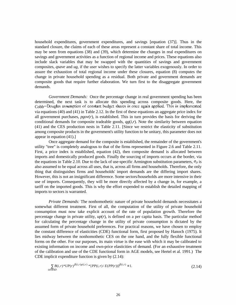
Private Demands: The nonhomothetic nature of private household demands necessitates asomewhat different treatment. First of all, the computation of the utility of private householdconsumption must now take explicit account of the rate of population growth. Therefore thepercentage change in private utility, up(r), is defined on a per capita basis. The particular methodfor calculating the percentage change in the utility of private consumption is dictated by theassumed form of private household preferences. For practical reasons, we have chosen to employthe constant difference of elasticities (CDE) functional form, first proposed by Hanoch (1975). Itlies midway between the nonhomothetic CES on the one hand, and the fully flexible functionalforms on the other. For our purposes, its main virtue is the ease with which it may be calibrated toexisting information on income and own-price elasticities of demand. (For an exhaustive treatmentof the calibration and use of the CDE functional form in AGE models, see Hertel et al. 1991.) TheCDE implicit expenditure function is given by (2.14):

(2.14)

27

Here, (E(⋅) represents the minimum expenditure required to attain a prespecified level of privatehousehold utility, UP(r), given the vector of private household prices, PP(r). Minimum expenditure�� 2� �� $�� &�� 3"i,r) andcombined in an additive �� 4�� 3 ��

minimum expenditure cannot be factored out of the left-hand side expression and (2.14) is animplicitly additive �� $�� 3

to replicate the desired compensated, own-price elasticities of demand, then choosing the 5��

replicate the targeted income elasticities of demand. (The shift term B(i,r) is a scale factor embodiedin the budget share, CONSHR(i,r), in the linearized representation of these preferences.)

Total differentiation of (2.14) and use of Shephard's lemma permits us to derive therelationship between minimum expenditure, utility, and prices that is given in equation (45) ofTable 2.12 (see also Hertel, Horridge, and Pearson 1992). Equation (46) determines per capitaprivate household demands for the tradeable composite commodities: qp(i,r) - pop(r). As long asEY(i,r) departs from unity, the pop(r) term does not cancel out, as it did in the case of homotheticgovernment and savings demands. Finally, in Table 2.12 we have a block of equations that developthe mix of composite consumption of tradeable commodities, based on domestic and compositeimported goods.

As noted in the previous paragraph, the parameters of the CDE function are initiallyselected (i.e., calibrated) to replicate a prespecified vector of own-price and income elasticities ofdemand. However, with the exception of some special cases of the CDE (e.g., the Cobb��!�

these elasticities are not constants. Rather, they vary with expenditure shares/relative prices. [SeeHertel et al. 1991 for derivations and more detailed discussion of these formulas. Chapter 4 alsoprovides illustrations of how the income elasticities of demand vary over expenditure levels.] Forthis reason we need some supplementary formulas describing how the elasticities are updated witheach iteration of the nonlinear solution procedure.

The formulas for the uncompensated price and income elasticities of demand, EP(i,k,r) andEY(i,r), are reported in Table 2.13. (These are not assigned equation numbers, as they are merelyused to compute parameter values to be used in the system of equations representing the model.$�� 6-�6! $�� )� ��

equal to one minus the CDE substitution parameter. (This simplifies some of the other formulas.) Formulas (F2) and (F3) compute the own� �� cross�� allen partial elasticities of substitution�� "$�� ! $�� ) ��

�� , �� &�� 3"i,r! ( 3 ∀i, then the cross-price elasticities of substitution are all�� + / 3 ( ) �� 7�8 �� 789 �� -�� &�� 3 ( +� ��

�� &�� 3 ( #� �� 7�� :�� premultipliedby CONSHR(i,r), formula (F3) yields the compensated, own-price elasticity of demand forcommodity i. Once these have been specified, this linear system of equations may be solved for the6��6 �� )� �� 3� �� "-+!� "9�� 7��

calibration procedures.)Formula (F4) shows how the income elasticities of demand are computed as a function of

consumption shares, the income expansion parameters, 5�� )�� ;��

of the own-price elasticities of demand must precede calibration of the income elasticities. Finally,the two may be combined to yield the uncompensated, own-price elasticities of demand reported in(F5).

28

Imperfect Factor Mobility

The two equations in Table 2.14 describe the responsiveness of imperfectly mobile factorsof production to changes in the rental rates associated with those sectors in which these sluggishfactors are employed. The mobility of these endowments is described with a CET revenue function(Powell and Gruen 1968), which is completely analogous to the CES cost functions used above,

except the revenue function is convex in prices. Thus the elasticity of transformation is nonpositive,*T < 0. As *T becomes larger in absolute value, the degree of sluggishness diminishes and there is atendency for rental rates across alternative uses to move together. As with the CES nests discussedabove, the first equation (50) introduces a price index and the second equation (51) determines thetransformation relationships. Note also that equation (51) is where we introduce the slack variable,to be used in those cases where the user wishes to fix the market price of a sluggish endowmentcommodity.

Macroeconomic Closure

Having described the structure of final demand, as well as factor market closure in theGTAP model, it remains to discuss the determination of aggregate investment. Like mostcomparative static AGE models, GTAP does not account for macroeconomic policies and monetaryphenomena, which are the usual factors explaining aggregate investment. Rather, we are concernedwith simulating the effects of trade policy and resource-related shocks on the medium term patternsof global production and trade. Because this model is neither an intertemporal model (e.g.,McKibbin and Sachs 1991), nor sequenced through time to obtain a series of temporary equilibria(e.g., Burniaux and van der Mensbrugghe 1991), investment does not come "on-line" next period toaffect the productive capacity of industries/regions in the model. However, a reallocation ofinvestment across regions will affect production and trade through its effects on the profile of finaldemand. Therefore, it is important to give this some attention. Also, a proper treatment of thesavings��

assuring consistency in our accounting.Because there is no intertemporal mechanism for determination of investment, we face

what Sen (1963) defined as a problem of macroeconomic closure [see also Taylor and Lysy(1979)]. Following Dewatripont and Michel (1987), we note that there are four popular solutions tothe fundamental indeterminacy of investment in comparative static models. The first three arenonneoclassical closures in which investment is simply fixed and another source of adjustment ispermitted. In the fourth closure investment is permitted to adjust; however, rather than including anindependent investment relationship, it simply accommodates any change in savings.

In addition to adopting a closure rule with respect to investment, it is necessary to come togrips with potential changes in the current account. Many multiregion trade models have evolved asa set of single-region models that are linked via bilateral merchandise trade flows [e.g., earlyversions of the SALTER model, which evolved from the ORANI model of Australia; see alsoLewis, Robinson, and Wang (1995)]. These models have no global closure with respect to savingsand investment, but instead impose the macroeconomic closure at the regional level. Here it iscommon to force domestic savings and investment to move in tandem, by fixing the current accountbalance. To understand this, it is useful to recall the following accounting identity, e.g., Dornbusch1980, which follows from equating national expenditure from the sources and uses sides:

29

M- R + X I - S ≡ (2.15)

which states that the national savings (S) minus investment (I) is identically equal to the currentaccount surplus, where R is international transfer receipts. (In the GTAP data base we do not haveobservations on R, so it is set equal to zero and S is derived as a residual, which reflects nationalsavings, net f the unobserved transfers.) By fixing the right-hand side of identity (2.15) one alsofixes the difference between national savings (including government savings) and investment. Thismay be accomplished in the GTAP framework by fixing the trade balance [DTBAL(r) = 0, seeequation (98) in Table 2.18] and freeing up either national savings [endogenize saveslack(r) inequation (38)] or investment [endogenize cgdslack(r) in equation (11′)].

If global savings equals global investment in the initial equilibrium, then the summationover the left-hand side of equation (2.15) equals zero and the sum of all current account balancesmust initially be zero (provided cif/fob margins are accounted for in national exports). Furthermore,by fixing the right-hand side of (2.15) on a regional basis, each region's share in the global pool ofnet savings is fixed. In this way, equality of global savings and investment in the new equilibrium isalso assured, in spite of the fact that there is no "global bank" to intermediate formally betweensavings and investment on a global basis. Finally, since investment is forced to adjust in line withregional changes in savings, this approach clearly falls within the "neoclassical" closure, asidentified by Dewatripont and Michel (1987).

The exogeneity of the current account balance embodies the notion that this balance is amacroeconomic, rather than microeconomic, phenomenon: to a great extent, the causality in identity(2.15) runs from the left side to the right side. It also facilitates analysis by forcing all adjustment toexternal imbalance onto the current account. If savings does not enter the regional utility function(as is the case in most multiregion AGE models outside of GTAP), this is also the right approach towelfare analysis because an arbitrary shift away from savings toward current consumption andincreased imports would otherwise permit an increase in utility to be attained, even in the absenceof improvements in efficiency or regional terms of trade.

For some types of experiments, however, modelers may wish to endogenize the balances oneither side of identity (2.15). For example, some trade policy reforms raise returns to capital and/orlower the price of imported capital goods. In this case, we would expect the increased rate of returnon new investment to result in an increase in regional investment and, ceteris paribus, adeterioration in the current account. In other cases one might wish to explore the implications of,for example, an exogenous increase in foreign direct investment, which would also dictate adeterioration in the current account. Once the left-hand side of (2.15) is permitted to adjust, amechanism is needed to ensure that the global demand for savings equals the global demand forinvestment in the postsolution equilibrium. The easiest way to do so is through the use of a "globalbank" to assemble savings and disburse investment. This is the approach that we adopt here.

The global bank in the GTAP model uses receipts from the sale of a homogeneous savingscommodity to the individual regional households in order to purchase (at price PSAVE) shares in aportfolio of regional investment goods. The size of this portfolio adjusts to accommodate changes inglobal savings. Therefore, the global closure in this model is neoclassical. However, on a regionalbasis, some adjustment in the mix of investment is permitted, thereby adding another dimension tothe determination of investment in the model.

30

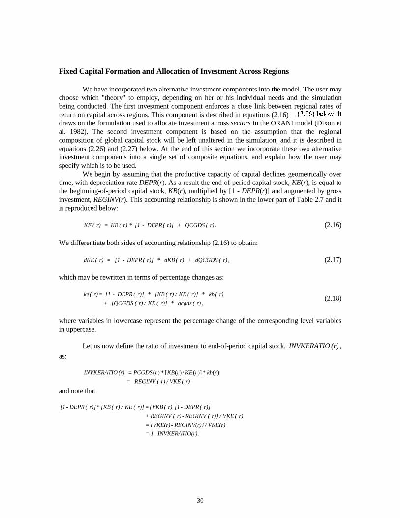
Fixed Capital Formation and Allocation of Investment Across Regions

We have incorporated two alternative investment components into the model. The user maychoose which "theory" to employ, depending on her or his individual needs and the simulationbeing conducted. The first investment component enforces a close link between regional rates ofreturn on capital across regions. This component is described in equations (2.16) � "��<! ��&� ,

draws on the formulation used to allocate investment across sectors in the ORANI model (Dixon etal. 1982). The second investment component is based on the assumption that the regionalcomposition of global capital stock will be left unaltered in the simulation, and it is described inequations (2.26) and (2.27) below. At the end of this section we incorporate these two alternativeinvestment components into a single set of composite equations, and explain how the user mayspecify which is to be used.

We begin by assuming that the productive capacity of capital declines geometrically overtime, with depreciation rate DEPR(r). As a result the end-of-period capital stock, KE(r), is equal tothe beginning-of-period capital stock, KB(r), multiplied by [1 - DEPR(r)] and augmented by grossinvestment, REGINV(r). This accounting relationship is shown in the lower part of Table 2.7 and itis reproduced below:

. r) ( QCGDS +r)] ( DEPR - [1* r) ( KB = r) ( KE (2.16)

We differentiate both sides of accounting relationship (2.16) to obtain:

,r) ( dQCGDS + r) ( dKB* r)] ( DEPR - [1 = r) ( dKE (2.17)

which may be rewritten in terms of percentage changes as:

,r) ( qcgds* r)] ( KE / r) ( [QCGDS +

r) ( kb* r)] ( KE / r) ( [KB* r)] ( DEPR - [1 =r) ( ke(2.18)

where variables in lowercase represent the percentage change of the corresponding level variablesin uppercase.

Let us now define the ratio of investment to end-of-period capital stock, (r) INVKERATIO ,as:

r) ( VKE / r) ( REGINV =

rkbrKErKBrPCGDS (r) INVKERATIO )(*)](/)([*)(=

and note that

. (r)INVKERATIO - 1=

VKE(r) / REGINV(r)} - {VKE(r)=

r) ( VKE / r)} ( REGINV - r) ( REGINV +

r)] ( DEPR - [1 r) ( {VKB =r)] ( KE / r) ( [KB* r)] ( DEPR - [1

31

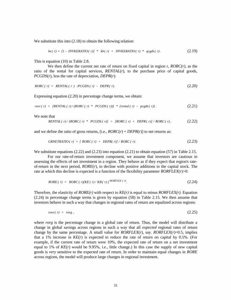
We substitute this into (2.18) to obtain the following relation:

. r) ( qcgds* r) ( INVKERATIO + r) ( kb* r)] ( INVKERATIO - [1 = r) ( ke (2.19)

This is equation (10) in Table 2.8.We then define the current net rate of return on fixed capital in region r, RORC(r), as the

ratio of the rental for capital services, RENTAL(r), to the purchase price of capital goods,PCGDS(r), less the rate of depreciation, DEPR(r):

. r) ( DEPR - r) ( /PCGDS ) r ( RENTAL = r) ( RORC (2.20)

Expressing equation (2.20) in percentage change terms, we obtain:

.r)] ( pcgds - r) ( [rental* r))] ( PCGDS* r) ( (RORC / r) ( [RENTAL = r) ( rorc (2.21)

We note that ,r) ( RORC /r)] ( DEPR + r) ( [RORC =r)] ( PCGDS* r) ( [RORC / r) ( RENTAL (2.22)

and we define the ratio of gross returns, [i.e., RORC(r) + DEPR(r)] to net returns as:

. r) ( RORC /r)] DEPR( + r) ( RORC [ = r) ( GRNETRATIO (2.23)

We substitute equations (2.22) and (2.23) into equation (2.21) to obtain equation (57) in Table 2.15.For our rate-of-return investment component, we assume that investors are cautious in

assessing the effects of net investment in a region. They behave as if they expect that region's rate-of-return in the next period, RORE(r), to decline with positive additions to the capital stock. Therate at which this decline is expected is a function of the flexibility parameter RORFLEX(r)>0:

. ]r) ( KB / r) ( r)[KE ( RORC = r) ( RORE r) ( -RORFLEX (2.24)

Therefore, the elasticity of RORE(r) with respect to KE(r) is equal to minus RORFLEX(r). Equation(2.24) in percentage change terms is given by equation (58) in Table 2.15. We then assume thatinvestors behave in such a way that changes in regional rates of return are equalized across regions:

,rorg = r) ( rore (2.25)

where rorg is the percentage change in a global rate of return. Thus, the model will distribute achange in global savings across regions in such a way that all expected regional rates of returnchange by the same percentage. A small value for RORFLEX(r), say. RORFLEX(r)=0.5, impliesthat a 1% increase in KE(r) is expected to reduce the rate of return on capital by 0.5%. (Forexample, if the current rate of return were 10%, the expected rate of return on a net investmentequal to 1% of KE(r) would be 9.95%, i.e., little change.) In this case the supply of new capitalgoods is very sensitive to the expected rate of return. In order to maintain equal changes in ROREacross regions, the model will produce large changes in regional investment.

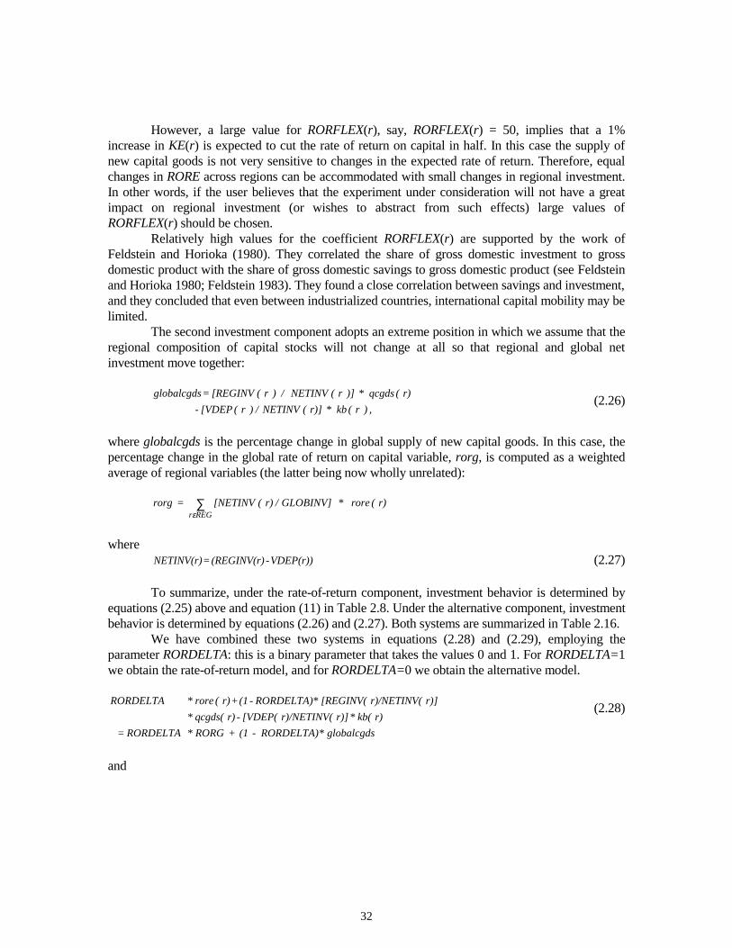
32

However, a large value for RORFLEX(r), say, RORFLEX(r) = 50, implies that a 1%increase in KE(r) is expected to cut the rate of return on capital in half. In this case the supply ofnew capital goods is not very sensitive to changes in the expected rate of return. Therefore, equalchanges in RORE across regions can be accommodated with small changes in regional investment.In other words, if the user believes that the experiment under consideration will not have a greatimpact on regional investment (or wishes to abstract from such effects) large values ofRORFLEX(r) should be chosen.

Relatively high values for the coefficient RORFLEX(r) are supported by the work ofFeldstein and Horioka (1980). They correlated the share of gross domestic investment to grossdomestic product with the share of gross domestic savings to gross domestic product (see Feldsteinand Horioka 1980; Feldstein 1983). They found a close correlation between savings and investment,and they concluded that even between industrialized countries, international capital mobility may belimited.

The second investment component adopts an extreme position in which we assume that theregional composition of capital stocks will not change at all so that regional and global netinvestment move together:

,) r ( kb* r)] ( NETINV / ) r ( [VDEP -

r) ( qcgds* )] r ( NETINV / ) r ( [REGINV = globalcgds(2.26)

where globalcgds is the percentage change in global supply of new capital goods. In this case, thepercentage change in the global rate of return on capital variable, rorg, is computed as a weightedaverage of regional variables (the latter being now wholly unrelated):

r) ( rore* GLOBINV] / r) ( [NETINV = rorgREGr∑

ε

whereVDEP(r)) - (REGINV(r) = NETINV(r) (2.27)

To summarize, under the rate-of-return component, investment behavior is determined byequations (2.25) above and equation (11) in Table 2.8. Under the alternative component, investmentbehavior is determined by equations (2.26) and (2.27). Both systems are summarized in Table 2.16.

We have combined these two systems in equations (2.28) and (2.29), employing theparameter RORDELTA: this is a binary parameter that takes the values 0 and 1. For RORDELTA=1we obtain the rate-of-return model, and for RORDELTA=0 we obtain the alternative model.

globalcgds* RORDELTA) - (1 +RORG * RORDELTA =

r) kb(* r)] r)/NETINV( [VDEP( - r) qcgds(*

r)] r)/NETINV( [REGINV(*RORDELTA) - (1 + r) ( rore* RORDELTA(2.28)

and

33

(r) rore* GLOBINV] / r) ( [NETINV* RORDELTA) - 1 ( +

(r) kb* V] (r)/GLOBIN [VDEP - r) ( qcgds*

GLOBINV] / r) ( [REGINV* RORDELTA =

rorg* RORDELTA) - 1 ( + globalcgds* RORDELTA

REGr

REGr

∑

∑

ε

ε}{

(2.29)

Equation (2.28) is shown in Table 2.15 as equation (59), and equation (2.29) is shown in Table 2.15as equation (11´). It replaces equation (11) in Table 2.8.

Once the level of investment activity in each region has been determined, it remains only togenerate the mix of expenditures for domestic and imported inputs used in the production of fixedcapital in region r: VDFA(i,"cgds",r) and VIFA(i,"cgds",s,r), respectively. This is completelyanalogous to the production of tradeable commodities. In fact, the same equations are used togenerate these derived demands. We assume that a unit of capital for investment in region r iscreated by assembling composite intermediate inputs in fixed proportions [equation (36) in Table2.11]. The composite intermediate input is, in turn, a CES combination of domestic and foreignimported inputs [equations (31) and (32) in Table 2.11 and equation (29) in Table 2.10]. However,in contrast to the production of tradeable commodities, capital creation requires no services ofprimary factors. This is because it is a fictitious activity that merely assembles goods destined forfixed investment in region r. In other words, the use of land, labor, and capital associated withcapital formation is already embodied in the intermediate inputs assembled by this investmentsector.

Global Transportation

In addition to the global bank, another global activity is required in this model in order tointermediate between the supply of, and demand for, international transport services. These servicesare provided via a Cobb��

from each region. Lacking the data to link exports of transport services with specific routes, wesimply combine these services into a single composite international transport good, the value ofwhich is VT = QT * PT. The percentage change equation for the composite price index was given inequation (7) of Table 2.8. For convenience, it is repeated as equation (7´) in Table 2.17. Recall thatthis is akin to a zero profit condition for the aggregate transport sector. The next equation (61) inTable 2.17 derives the conditional demands for the inputs to the shipping services sector, assumingthat the share of each region in the global industry is constant, that is, Cobb��

Therefore, this equation includes an expansion effect (qt) and a substitution effect, whereby theelasticity of substitution is assumed to be unitary.

The next two equations in Table 2.17 refer to the uses of the composite internationalshipping service. We assume that this composite is employed in fixed proportions with the volumeof a particular good shipped along a particular route, QXS(i,r,s). In other words: ATR(i,r,s) *QTS(i,r,s) = QXS(i,r,s), where QTS(i,r,s) is the amount of the homogeneous product QT used inshipping commodity i from r to s, and ATR(i,r,s) is a technical coefficient. Equilibrium in the globaltransport services market therefore requires that:

. QT = s)r, i, ( QTSREGsREGrTRADi∑∑∑

εεε(2.30)

34

Proportionately differentiating this equation gives:

. qt* QT = s)r, i, ( qts* s)r, i, ( QTSREGsREGrTRADi∑∑∑

εεε(2.31)

Multiplying both sides by the common price of the composite transport service, and substituting[qxs(i,r,s) - atr(i,r,s)] for qts(i,r,s) gives equation (62) in Table 2.17. The presence of atr(i,r,s) inthis formulation permits the user to introduce commodity/route-specific technical change ininternational transport services. This also requires us to modify the fob/cif price linkage equation(26) in Table 2.9 to reflect the fact that an increase in efficiency along a particular route will lowercif values, for a given fob price. This revision is reported in (26´) of Table 2.17.

Summary Indices

This section discusses the summary indices computed in the GTAP model. These equationsdo not play a role in determining the equilibrium solution. Indeed, all these indices could becomputed after the fact. However, it is convenient to include them in the model so that their rates ofchange are reported along with the other results. Table 2.18 shows aggregate indices of pricesreceived [psw(r), equation (64)] and prices paid [pdw(r), equation (65)] for products sold andpurchased by each region (inclusive of savings and investment, which represent transactions withthe global bank). The difference between psw(r) and pdw(r) measures the percentage change ineach region's terms of trade, tot(r).

GTAP also computes regional equivalent variation measures, EV(r), which arise due to thesimulation under consideration. The values for EV(r) are in 1992 $US million, and they arecomputed as:8

EV(r) = u(r) * INC(r)/100.

Since u(r) reports per capita welfare, equation (67) in Table 2.18 also includes the rate of change inpopulation on the right�� EV reported by the model represents total regionalwelfare. The worldwide equivalent variation (WEV) is then computed as the simple summation ofthe regional EVs, equation (68). This is followed by an equation generating the percentage in theregion-specific consumer price index, ppriv(r).

Other useful price and quantity indices included in GTAP refer to trade, regional grossdomestic product (GDP), and income magnitudes. To obtain quantity indices, it is necessary tocompute the corresponding value and price indices first, because we are aggregating over differentcommodities. For example, variable qgdp(r), equation (72) of Table 2.18, is a quantity index fordomestic product.9 Table 2.18 shows that we first compute a value index, vgdp(r), in equation (70),which accounts for changes in prices and quantities, and a price index, pgdp(r), in equation (71),which accounts for changes in prices only. The quantity index, qgdp(r), is then computed as thedifference between vgdp(r) and pgdpr(r). For simulations of trade and domestic policy changes, thesolution value for qgdp(r) will typically be small, reflecting only shifts in the economy's productionpossibilities frontier owing to the improved allocation of a fixed resource base. But for simulationsof endowment growth, the solution value for qgdp(r) will provide a summary measure of growth forthe region.

35

We next turn to a set of equations defining changes in aggregate trade values, prices andquantity indices. Equations (73)�"=>! �� 1

(1) by commodity and region, (2) by region for all traded commodities, and (3) by commodity forall regions in the world. Equation (79) computes the percentage change in the value of total worldtrade, and equation (80) computes the percentage in value of world output, by commodity.10 Theseare followed by eight analogous equations, (81)�">>!� &��

after which we are able to extract pure volume changes for aggregate trade and output [equations(89)�"%<!?�

The last two equations in the model are given at the bottom of Table 2.18. They are used tocompute the change in trade balance, by commodity and by region. This is a value-based concept,and DTBAL(r), equation (98) refers to the changes in the current account for each region.

VII. A SIMPLE NUMERICAL EXAMPLE

Perhaps the best way to understand how this model works is to perform a simpleexperiment and examine the resulting changes in endogenous variables of interest. (This is example21 in the Hands-On document, referred to in Chapter 6, and available through the Web site.) Inorder to keep things simple, we will work with a three-commodity/three-region aggregation of thedata base. The three commodities are: food, manufactures, and services. The three regions are: theUnited States (US), the European Union (EU) and the rest of the world (ROW). The experimentinvolves a bilateral reduction in the level of the EU's import tariff on US food products. Inparticular, tms(food,usa,eu) = -10%. This implies a cut of 10% in the power of the ad valorem tariff,which amounts to a 10% cut in the domestic price of US food exports to the EU, ceteris paribus.Furthermore, we begin by performing only the first step in a multistep solution of the modeldeveloped above. In terms of Figure 2.5, this means we are moving from (X0, Y0) to (X1, YJ), whereYJ is a Johansen approximation to Y1 (the true solution). This is merely a pedagogical device tofacilitate discussion of our example, since in the Johansen solution, the linearized form of the modelin Tables 2.8��+> &�� hold exactly. For small shocks this may provide a reasonable approximationto the true, nonlinear price and quantity changes. However, it is a very poor method for assessingwelfare changes [see Hertel, Horridge, and Pearson (1992) for an extensive discussion of theseissues]. The reader can observe this approximation error by comparing the Johansen solution withthe Gragg outcomes (given in brackets) in Tables 2.20, 2.22, and 2.23.

Tables 2.19 and 2.20 report selected changes in the EU, resulting from the bilateral tariffcut. We begin at the top of the table, with the market price of US food in the US. This market pricerises by 0.140% due to increased demand. Since there is no change in the border tax, pfob rises bythe same amount, via equation (27) in Table 2.9. The cif price of US food exports to the EUdepends also on changes in the price index of international transport services, pt. This drops slightlydue to the decline in the price of EU transport services [Table 2.19 and equation (7)]. Therefore,pcif increases by a slightly smaller amount.

The bilateral tariff instrument, which is the subject of this experimental shock, enters viaequation (24) in Table 2.9. Its reduction serves to lower the domestic market price of EU foodimports from the US by an additional 10%, so that pms(food,usa,eu) = -9.876%. This price cut hastwo immediate effects. First, it lowers the price of composite imports by 1.631% [equation (28) inTable 2.10], a value that is roughly equal to the share of US imports in total expenditures onimported food multiplied by -9.876%. The second immediate effect of this price cut is that it

36

encourages agents in the EU to alter their sourcing of food imports in favor of US products[equation (29) in Table 2.10]. The responsiveness of this shift in the model is dictated by theelasticity of substitution among food imports (*M). Its value in the aggregated data base is 4.64. Thisfigure is multiplied by the percentage change in the cost of food imports from the US, relative tocomposite import costs, or the difference in these two individual percentage changes. This equals38.26%. If the level of imports qim were unchanged, this would be the end of the story. However,the impact of the bilateral cut in protection continues, since the cheaper imports result in asubstitution of composite imports for domestic food. This effect varies by sector in this model, dueto the differing importance of imports in the composite intermediate good. Since the substitutionstructure in each of these is very similar, we choose to focus on the EU food industry, which is thelargest user, accounting for 52.7% of total food imports in that market. In this industry, aggregateimports increase by 3.18%. Thus the total increase in US food imports by the EU food industry is equal to 41.4%.

The numerical implementations of equations (30) and (31) in Table 2.11 describe thechanges at the next level of the production tree (recall Figure 2.3). They account for the 3.0%increase in composite food imports by this sector. However, note from equation (31) that in thiscase the expansion and substitution effects work in opposite directions, since qf(food,eu) =qo(food,eu) < 0. That is, the food sector as a whole contracts, and with it, there is a decline in thedemand for intermediate products, in this case food. Equation (32) shows that the demand fordomestically produced intermediates actually falls. Finally, owing to a decline in the total demandfor domestically produced food, the price of EU-produced food falls.

Table 2.20 reports selected price and quantity changes for the EU as a whole, owing to thisbilateral tariff cut. The price of farmland falls, since this factor has no alternative uses outside of thefood sector in our model, and output in that sector has declined. With labor and capital beingreleased from the food sector, the nonfood sectors are able to expand. In general equilibrium,households increase their consumption of all nonsavings commodities due to the lower prices. Thedemand for savings falls, since its price is determined by a weighted combination of the capitalgoods prices from all regions, which tend to rise relatively more than other goods prices.

Now turn to the effects of the tariff cut on the US economy, which are reported in Tables2.21 and 2.22. Equation (1) in Table 2.21 combines the increase in US�84 �� &��

changes in sales to other destinations/uses in order to estimate the change in food sector output inthe US. The first figures in parentheses are the shares of sales to various uses. From this, it can beseen that exports to the EU account for only 1.3% of the value of total US food sector output (atdomestic market prices). This considerably tempers the impact of the 41.4% increase in sales. Ofcourse the importance of this market for selected, disaggregated producer groups can be muchlarger, and might warrant strategic disaggregation of the data base to capture such effects.

It is not surprising that the bulk of US food sales goes to the domestic market (92.6%).However, it is somewhat surprising that the tariff cut in the EU causes domestic sales of US food toincrease. More insight into this result may be obtained by considering the numericalimplementation of equation (3) in Table 2.21. This shows the changes in composition of domesticsales. As expected, sales to other industries and final demand fall, as US supply prices for food arebid up by the EU users. However, these declines are more than offset by an increase in intermediatedemands for food in the US food sector. In other words, to meet the increased demand for food inthe EU, domestic sales of intermediate goods must also increase.

Table 2.22 describes the economywide effects of the bilateral tariff cut on the US. Here, theland rental rate rises by more than the food price, and labor and capital wages rise by somewhat

37

less, with the relative capital intensity of the food sector favoring capital over labor. Continuing theanalogy, we see that the manufacturing sector must contract in order to make way for expansion ofthe US food sector. Finally, note that composite consumption of nonfood manufactures and servicesincreases, as households substitute imported for domestic goods.

The final table, Table 2.23, summarizes the macroeconomic effects of the EU's bilateraltariff cut. The increase in demand for US products bids up US prices, relative to the prices ofproducts supplied from the EU and ROW. Since the EU must export more products to pay for theincrease in food imports, their export volume increases by .233%, in the case where RORDELTA =0 and a simple Johansen solution is used. (See the top entry in the second column of Table 2.23.) Therefore, the EU supply prices must fall relative to other regions. This results in a terms-of-tradedeterioration for the EU, as seen in the third row of Table 2.23. The terms-of-trade for ROW aremarginally worsened, due to displacement by US exporters. This translates into a welfare loss forROW. In the EU, the terms-of-trade decline is more than offset by the improved allocation ofdomestic resources, and aggregate regional welfare rises by $346 million. The US gains $778million due to its improved terms-of-trade, following the preferential cut in border taxes on US foodexports to the EU.

It is interesting to note that the trade balance hardly changes, DTBAL (r) @ #� ��

simulations where RORDELTA = 0. This is a robust outcome that follows from equation (2.15) andthe treatment of savings and investment in the model. The demand for savings is tied directly toincome, which is little affected in this (and most other) policy reform experiments. Since regionalsavings doesn't change much, global savings, and hence global investment, are unaltered. Therefore,the only means of altering the left-hand side of (2.15), (S - I), and hence the trade balance, is to alterthe regional allocation of investment. When RORDELTA = 0, this is not possible. Therefore, therecan be little change in the right-hand side of (2.15), (X - M).

This is no longer true, however, when RORDELTA = 1, and the global bank's allocation ofinvestment across regions is flexible. In the lower (parenthetical) entries of Table 2.23, we reportresults of the Johansen simulation with RORFLEX = 10 (the default setting for this parameter).Now changes in rate-of-return on investment come into play. From the second row of Table 2.23,we see that rorc(eu) < 0, since the rental rate on capital declines relative to the price of capitalgoods. Therefore, there is an incentive to divert some investment to other regions. Given S, theresulting decline in I requires an increase in (X - M) via identity (2.15). This is achieved by aslightly larger increase in export volume (.263% vs. .233%) from the EU, and a smaller increase inimports. Not surprisingly, this results in a stronger terms-of-trade deterioration and therefore asmaller gain in welfare, as opposed to the case where RORDELTA = 0.11

A comparison of the Johansen results with the nonlinear results (reported in brackets inTable 2.23) shows that the Johansen solution yields a poor approximation to the true welfare effectson the EU, even for this relatively small shock. This is because the change in EU utility reflects thedifference between two larger changes, one of which is positive (efficiency gains) and one of whichis negative (terms-of-trade effect). As can be seen from the third row of Table 2.23, the Johansensolution underestimates the true deterioration in the EU's terms of trade by a third. On the otherhand, this solution procedure tends to overstate the gains from elimination of a distortion.Therefore, it is not surprising that the gain in EU welfare is overstated by more than five times($346 million vs. the true gain of $62 million, reported in brackets). Indeed, it is not uncommon forsuch comparisons to yield sign reversals in some regions' welfare. In sum, use of the Johansen one-step solution procedure for purposes of decomposing small changes in prices and quantities (as inTables 2.19 and 2.21) is very useful. However, it is not an acceptable procedure for conducting

38

welfare analysis of policy reforms. For welfare analysis, the nonlinear solution procedures availablein GEMPACK must be used.

VIII. SUMMARY

This completes our summary of the structure of the GTAP model. For your convenience,we have assembled a glossary of notation used in the model. This is provided at the back of thisbook. As noted, the electronic file, GTAP94.TAB, contains a complete listing of the model code. Itis available on the FTP site. Access to this site is discussed in Chapter 6. The best way to becomefamiliar with the model is to apply it to a particular problem of interest. After covering the database, the parameters, aggregation, and computing issues, we will turn to a set of seven diverseapplications of this model.

39

NOTES

1. The authors would like to thank Martina Brockmeier for her development of much of this material.For a more extensive graphical exposition of the GTAP model, see Brockmeier (1996).

2. The motivation for including savings in this atemporal utility function derives from Howe (1975) andis discussed at greater length below.

3. In some cases the initial data base does not include taxation in these markets. However, the possibilityof introducing such taxation is available in the model, and it must therefore be accounted for in thecomputation of regional income.

4. The most natural way to implement this model would be via a mixed levels and percentage changerepresentation. Indeed, this is possible in GEMPACK (Harrison and Pearson 1994). However, it iscomputationally more burdensome. Also, by linearizing the accounting equations some additionalinsights may be obtained.

5. This type of nonlinear solution procedure is now the default option in GEMPACK. For an exhaustivecomparison of the linearized and levels approaches to AGE modeling, the reader is referred to Hertel,Horridge, and Pearson (1992).

6. For the user with an interest in applications for which intermediate��

intermediate��

tailoring it to the specific needs at hand. However, this is not particularly difficult, as will be seenbelow.

7. Howe (1975) also shows that the savings share parameter in the atemporal utility function can berelated to 1 one minus the ratio of consumer's rate of time preference to the rate of reproduction ofcapital.

8. The coefficient INC(r) reports initial equilibrium values for regional expenditure (which must equalincome).

9. Values for the coefficient gross domestic product, GDP(r), are computed as follows:G D P r V G A i r V P A i r V O A C G D S r

V X W D i r s V ST i r V IW S i r s

i TR AD

r RE Gi TR ADi TR ADs RE Gi TR AD

( ) [ ( , ) ( , )] (" " , )

( , , ) ( , ) ( , , )

= + +

+ + −

∑∑∑∑∑∑

ε

εεεεε

10. The coefficient VOW(i,r) measures the value of regional production at world prices, and its values arecomputed as follows: VOW(i,r) = VDM(i,r) * PW_PM(i,r) + ∑ REGs irsVXWDε )( . The coefficient

PW_PM(i,r) converts domestic use valued at market prices, VDM(i,r), to world prices, and it iscomputed as follows: P W P M i r V X W D i r s V X M D i r ss RE Gs RE G_ ( , ) ( , , ) / ( , , )= ∑∑ εε

11. The combination of RORDELTA = 1 and the Gragg nonlinear solution procedure actually gives aslight decline in EU welfare.

40

REFERENCES

Alston, J. M., C. A. Carter, R. Green, and D. Pick (1990) "Whither Armington Trade Models?"American Journal of Agricultural Economics 72(2):455� <=�

Armington, P. A. (1969) "A Theory of Demand for Products Distinguished by Place of Production,"IMF Staff Papers 16:159�+=>�

Arrow, K. J., H. B. Chenery, B. S. Minhas, and R. M. Solow (1961) "Capital-Labor Substitutionand Economic Efficiency," Review of Economics and Statistics 43:225��#�

Brockmeier, M. (1996) "A Graphical Exposition of the GTAP Model," GTAP Technical Paper,Center for Global Trade Analysis, Purdue University, West Lafayette, IN.

Brown, D. K. and R. M. Stern (1989) "U.S.�7�� ;�� $�� 8��1 $�� A��

Produce Differentiation and Market Structure." In R. C. Feenstra (ed.), Trade Policies forInternational Competitiveness. Chicago: University of Chicago Press.

Burniaux, J. M. and D. van der Mensbrugghe (1991) "Trade Policies in a Global Context: TechnicalSpecification of the Rural/Urban-North/South (RUNS) Applied General Equilibrium TradeModel," Technical Paper No. 48, Paris, OECD, The Development Centre, November.

Dewatripont M., and G. Michel (1987) "On Closure Rules, Homogeneity and Dynamics in AppliedGeneral Equilibrium Models," Journal of Development Economics 26:65�=<�

Dixit, A. K. and J. E. Stiglitz (1979) "Monopolistic Competition and Optimum Product Diversity,"American Economic Review 67:297�'#>�

Dixon, P. B., B. R. Paramenter, J. Sutton, and D. P. Vincent (1982) Orani: A Multisectoral Modelof the Australian Economy New York: North Holland.

Dornbusch, R. (1980) Open Economy Macroeconomics New York: Basic Books.

Feenstra, R. C. (1994) "New Product Varieties and the Measurement of International Prices,"American Economic Review 84:157�+==�

Feldstein, M. (1983) "Domestic Savings and International Capital Movements in the Long Run andShort Run," European Economic Review 21:129�+�+�

Feldstein, M., and Charles Horioka (1980) "Domestic Savings and International Capital Flows,"Economic Journal 90:314�'�%�

Francois, J., B. McDonald, and H. Nordstrom (1995) "Assessing the Uruguay Round," paperpresented at the World Bank Conference on Developing Economies and the UruguayRound, January.

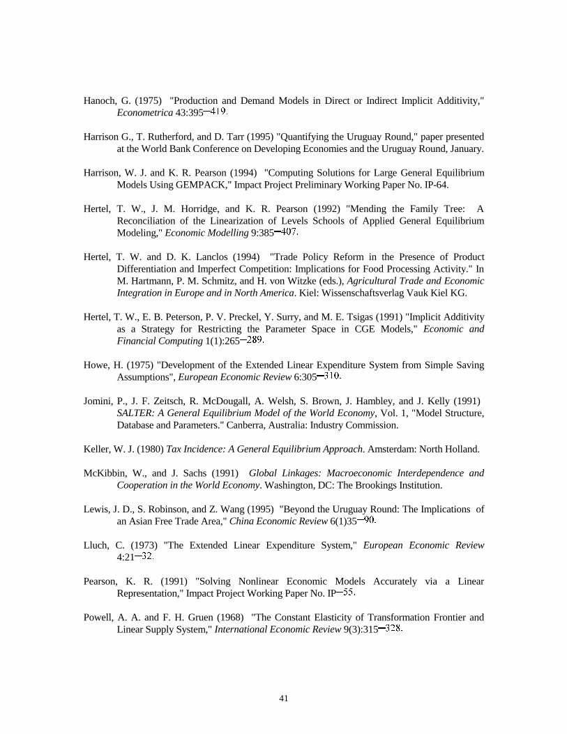
41

Hanoch, G. (1975) "Production and Demand Models in Direct or Indirect Implicit Additivity,"Econometrica 43:395� +%�

Harrison G., T. Rutherford, and D. Tarr (1995) "Quantifying the Uruguay Round," paper presentedat the World Bank Conference on Developing Economies and the Uruguay Round, January.

Harrison, W. J. and K. R. Pearson (1994) "Computing Solutions for Large General EquilibriumModels Using GEMPACK," Impact Project Preliminary Working Paper No. IP-64.

Hertel, T. W., J. M. Horridge, and K. R. Pearson (1992) "Mending the Family Tree: AReconciliation of the Linearization of Levels Schools of Applied General EquilibriumModeling," Economic Modelling 9:385� #=�

Hertel, T. W. and D. K. Lanclos (1994) "Trade Policy Reform in the Presence of ProductDifferentiation and Imperfect Competition: Implications for Food Processing Activity." InM. Hartmann, P. M. Schmitz, and H. von Witzke (eds.), Agricultural Trade and EconomicIntegration in Europe and in North America. Kiel: Wissenschaftsverlag Vauk Kiel KG.

Hertel, T. W., E. B. Peterson, P. V. Preckel, Y. Surry, and M. E. Tsigas (1991) "Implicit Additivityas a Strategy for Restricting the Parameter Space in CGE Models," Economic andFinancial Computing 1(1):265��>%�

Howe, H. (1975) "Development of the Extended Linear Expenditure System from Simple SavingAssumptions", European Economic Review 6:305�'+#�

Jomini, P., J. F. Zeitsch, R. McDougall, A. Welsh, S. Brown, J. Hambley, and J. Kelly (1991) SALTER: A General Equilibrium Model of the World Economy, Vol. 1, "Model Structure,Database and Parameters." Canberra, Australia: Industry Commission.

Keller, W. J. (1980) Tax Incidence: A General Equilibrium Approach. Amsterdam: North Holland.

McKibbin, W., and J. Sachs (1991) Global Linkages: Macroeconomic Interdependence andCooperation in the World Economy. Washington, DC: The Brookings Institution.

Lewis, J. D., S. Robinson, and Z. Wang (1995) "Beyond the Uruguay Round: The Implications ofan Asian Free Trade Area," China Economic Review 6(1)35�%#�

Lluch, C. (1973) "The Extended Linear Expenditure System," European Economic Review4:21�'��

Pearson, K. R. (1991) "Solving Nonlinear Economic Models Accurately via a LinearRepresentation," Impact Project Working Paper No. IP��

Powell, A. A. and F. H. Gruen (1968) "The Constant Elasticity of Transformation Frontier andLinear Supply System," International Economic Review 9(3):315�'�>�

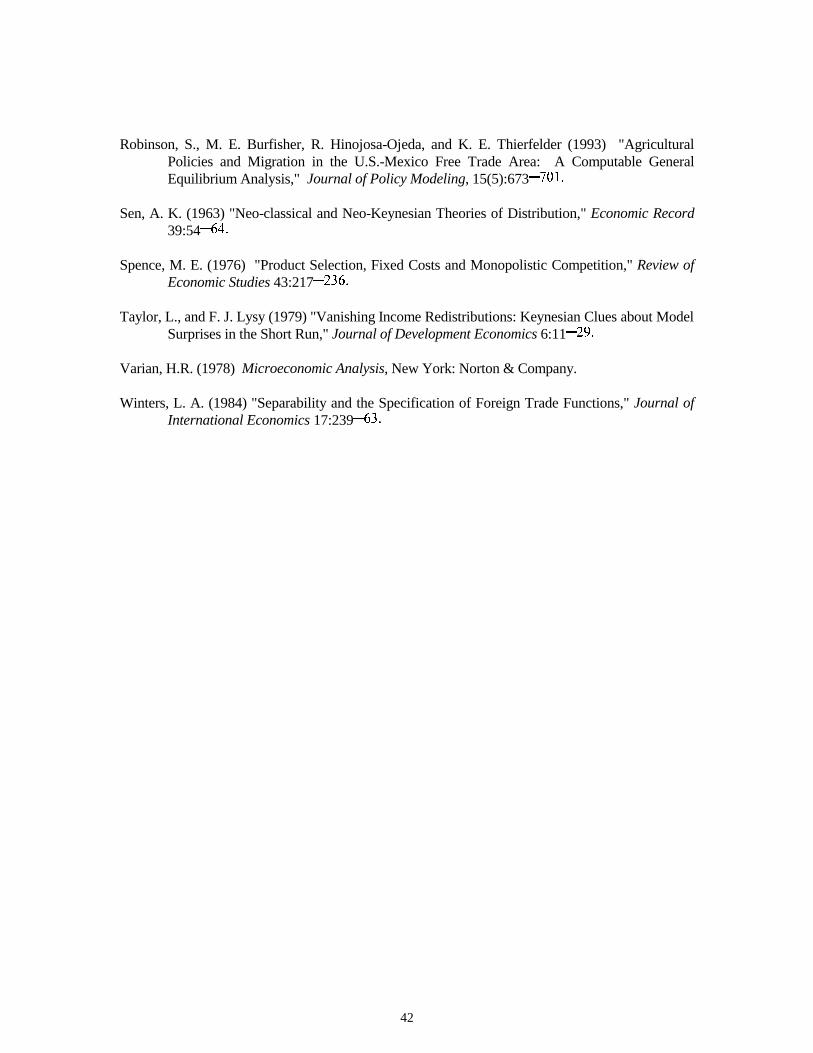
42

Robinson, S., M. E. Burfisher, R. Hinojosa-Ojeda, and K. E. Thierfelder (1993) "AgriculturalPolicies and Migration in the U.S.-Mexico Free Trade Area: A Computable GeneralEquilibrium Analysis," Journal of Policy Modeling, 15(5):673�=#+�

Sen, A. K. (1963) "Neo-classical and Neo-Keynesian Theories of Distribution," Economic Record39:54�< �

Spence, M. E. (1976) "Product Selection, Fixed Costs and Monopolistic Competition," Review ofEconomic Studies 43:217��'<�

Taylor, L., and F. J. Lysy (1979) "Vanishing Income Redistributions: Keynesian Clues about ModelSurprises in the Short Run," Journal of Development Economics 6:11��%�

Varian, H.R. (1978) Microeconomic Analysis, New York: Norton & Company.

Winters, L. A. (1984) "Separability and the Specification of Foreign Trade Functions," Journal ofInternational Economics 17:239�<'�

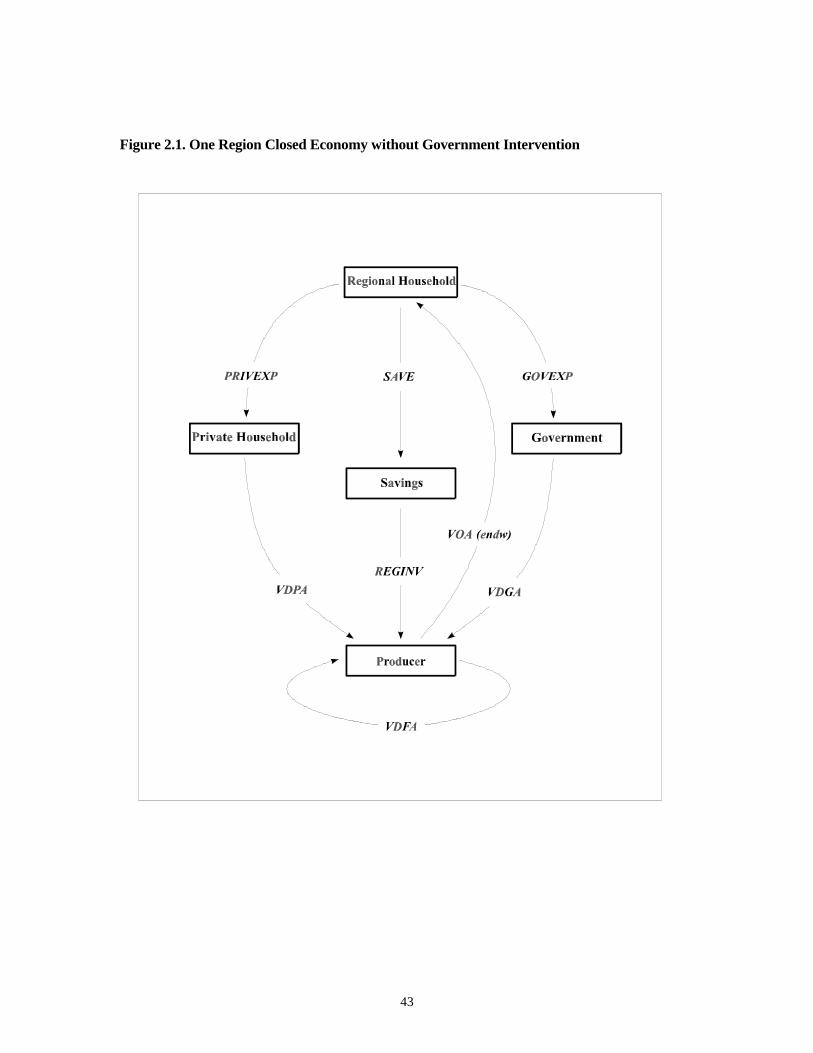
43

Figure 2.1. One Region Closed Economy without Government Intervention

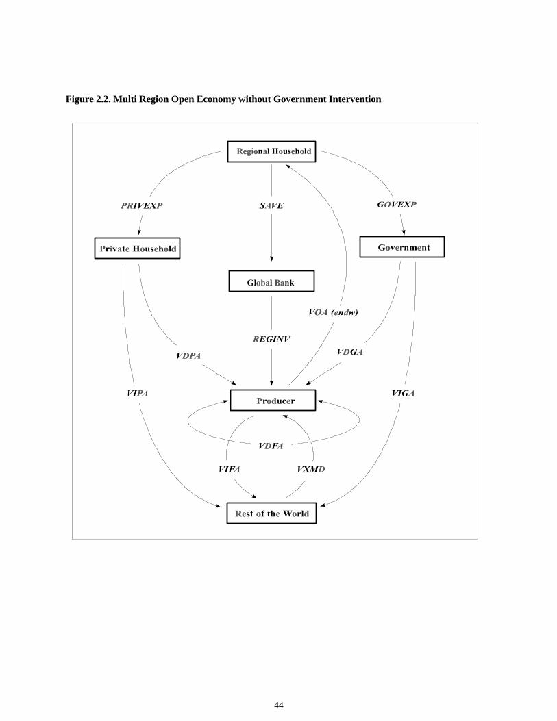
44

Figure 2.2. Multi Region Open Economy without Government Intervention

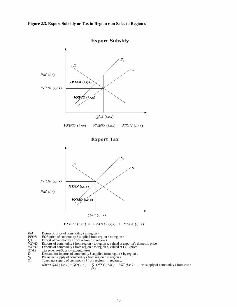
45

Figure 2.3. Export Subsidy or Tax in Region r on Sales to Region s

PM Domestic price of commodity i in region rPFOB FOB price of commodity i supplied from region r to region sQXS Export of commodity i from region r to region sVXWD Exports of commodity i from region r to region s, valued at exporter's domestic priceVXWD Exports of commodity i from region r to region s, valued at FOB priceXTAX Tax revenues/Subsidy expendituresD Demand for imports of commodity i supplied from region r by region sS0 Pretax net supply of commodity i from region r in region sS1 Taxed net supply of commodity i from region r in region s,

where: = ) r (i, VST - ) k r, i, ( QXS - ) r i, ( QO = ) sr, i, ( QXS s k

∑≠

1 net supply of commodity i from r to s

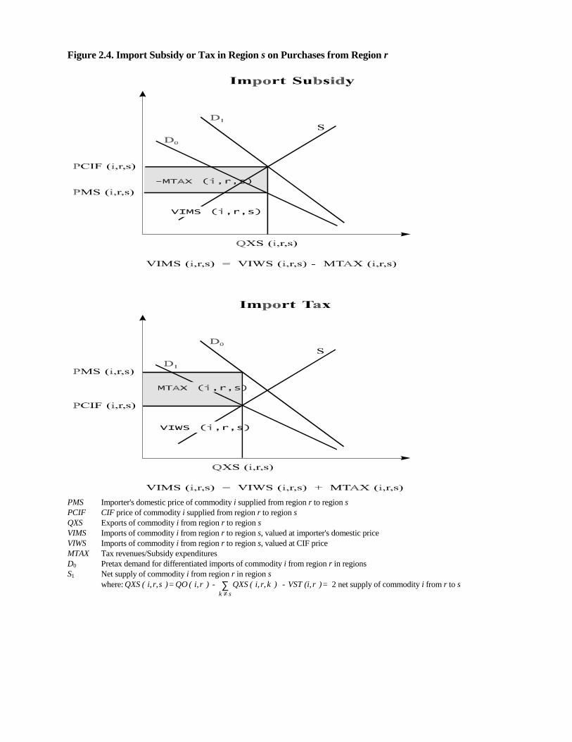
Figure 2.4. Import Subsidy or Tax in Region s on Purchases from Region r

PMS Importer's domestic price of commodity i supplied from region r to region sPCIF CIF price of commodity i supplied from region r to region sQXS Exports of commodity i from region r to region sVIMS Imports of commodity i from region r to region s, valued at importer's domestic priceVIWS Imports of commodity i from region r to region s, valued at CIF priceMTAX Tax revenues/Subsidy expendituresD0 Pretax demand for differentiated imports of commodity i from region r in regionsS1 Net supply of commodity i from region r in region s

where: = ) r (i, VST - ) k r, i, ( QXS - ) r i, ( QO = ) sr, i, ( QXS s k

∑≠

2 net supply of commodity i from r to s

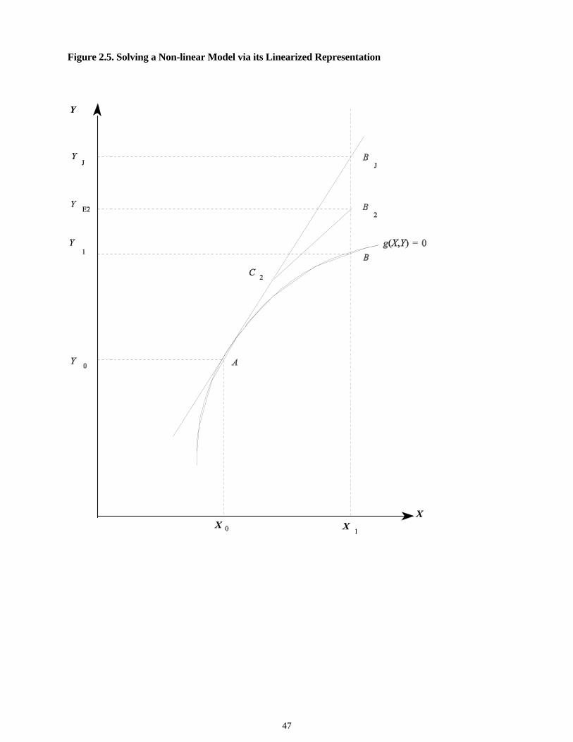
47

Figure 2.5. Solving a Non-linear Model via its Linearized Representation

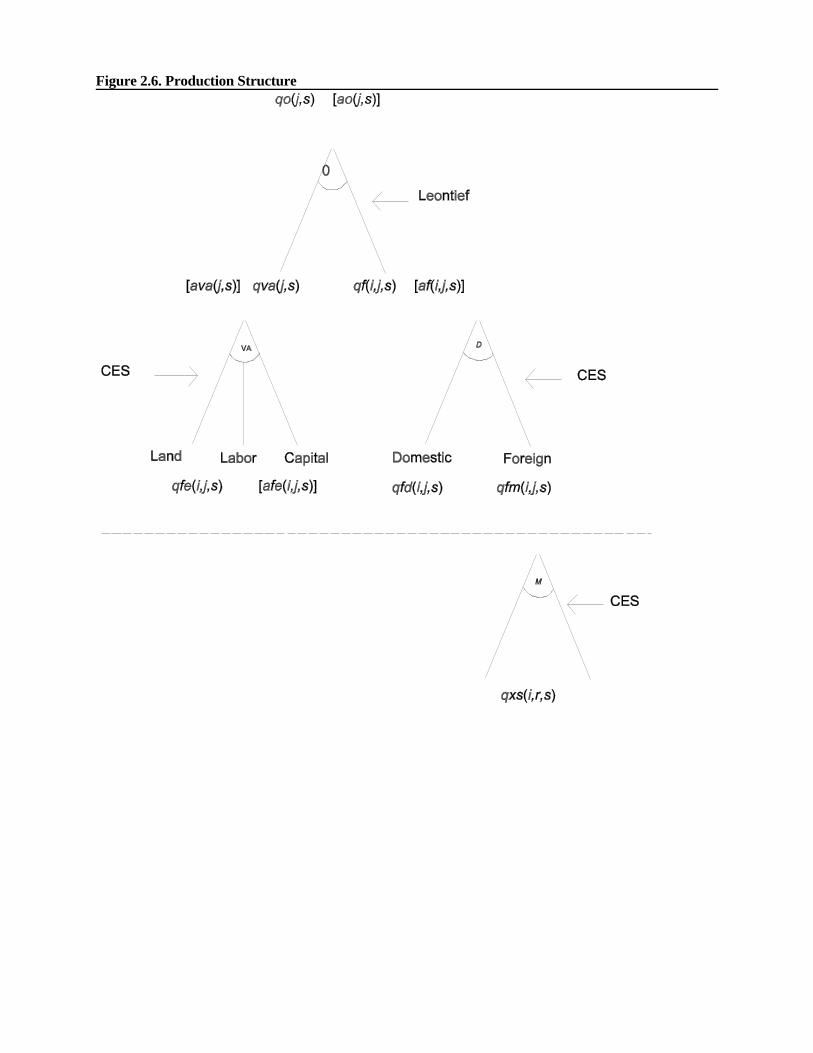
Figure 2.6. Production Structure

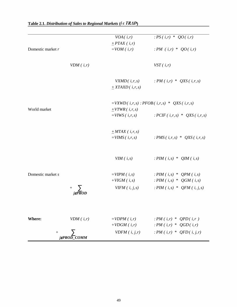
49

Table 2.1. Distribution of Sales to Regional Markets (� � ��)

r) i, ( VOA r) i, ( QO* r) i, ( PS :

+ r) i, ( PTAX

Domestic market r = r) i, ( VOM r) i, ( QO* r) i, ( PM :

r) i, ( VDM r) i, ( VST

s)r, i, ( VXMD s)r, i, ( QXS* r) i, ( PM:

+ s)r, i, ( XTAXD

= s)r, i, ( VXWD s)r, i, ( QXS* s)r, i, ( PFOB :

World market + s)r, i, ( VTWR

= s)r, i, ( VIWS s)r, i, ( QXS* s)r, i, ( PCIF :

+ s)r, i, ( MTAX

= s)r, i, ( VIMS s)r, i, ( QXS* s)r, i, ( PMS :

s)i, ( VIM s)i, ( QIM* s)i, ( PIM :

Domestic market s = s)i, ( VIPM s)i, ( QPM* s)i, ( PIM :

+ s)i, ( VIGM s)i, ( QGM* s)i, ( PIM :

+ ∑PRODjεεεε

s)j, i, ( VIFM s)j, i, ( QFM* s)i, ( PIM :

Where: r) i, ( VDM = r) i, ( VDPM ) r i, ( QPD* r) i, ( PM :

+ r) i, ( VDGM r) i, ( QGD* r) i, ( PM :

+ ∑PROD_COMMjεεεε

r) j, i, ( VDFM r) j, i, ( QFD* r) i, ( PM :

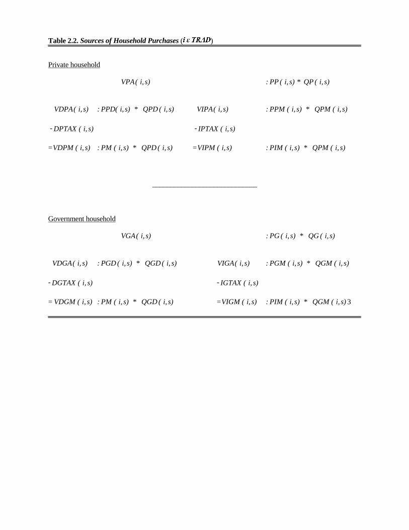
Table 2.2. Sources of Household Purchases (� � ��)

Private household

s)i, ( VPA s)i, ( QP* s)i, ( PP :

s)i, ( VDPA s)i, ( QPD* s)i, PPD( : s)i, ( VIPA s)i, ( QPM* s)i, ( PPM :

- s)i, ( DPTAX - s)i, ( IPTAX

= s)i, ( VDPM s)i, ( QPD* s)i, ( PM : = s)i, ( VIPM s)i, ( QPM* s)i, ( PIM :

_____________________________

Government household

s)i, ( VGA s)i, (QG * s)i, (PG :

s)i, ( VDGA s)i, ( QGD* s)i, ( PGD : s)i, ( VIGA s)i, ( QGM* s)i, ( PGM :

- s)i, ( DGTAX - s)i, ( IGTAX

= s)i, ( VDGM s)i, ( QGD* s)i, ( PM : = s)i, ( VIGM s)i, ( QGM* s)i, ( PIM : 3

51

Table 2.3. Sources of Firms' Purchases (� � ��)

� � ��: Intermediate inputs

s)j, i, ( VFA s)j, i, ( QF* s)j, i, ( PF :

s)j, i, ( VDFA s)j , i, ( QFD* s)j, i, ( PFD : s)j, i, ( VIFA s)j, i, ( QFM* s)j, i, ( PFM :

- s)j, i, ( DFTAX - s)j, i, ( IFTAX

= s)j, i, ( VDFM s)j, i, ( QFD* s)i, ( PM : = s)j, i, ( VIFM s)j, i, ( QFM* s)i, ( PIM :

� � �� : Primary factor services

s)j, i, ( VFA 4 s)j, i, ( QFE* s)j, i, ( PFE : 5

- s)j, i, ( ETAX 6

= s)j, i, ( VFM 7 s)j, i, ( QFE* s)i, ( PM : 8

Zero pure profits

s)j, i, ( VFA + s)j, i, ( VFA = s)j, ( VOAENDWiTRADi∑∑

εε

9

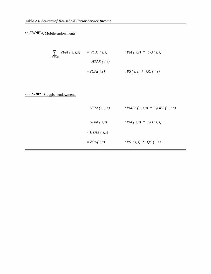
Table 2.4. Sources of Household Factor Service Income

� � ��: Mobile endowments

s)j, i, ( VFM PRODj∑

ε

= s)i, ( VOM s)i, ( QO* s)i, ( PM :

- s)i, ( HTAX

= s)i, ( VOA s)i, ( QO* s)i, ( PS :

� � ��: Sluggish endowments

s)j, i, ( VFM s)j, i, ( QOES* s)j, i, ( PMES :

s)i, ( VOM s)i, ( QO* s)i, ( PM :

- s)i, ( HTAX

= s)i, ( VOA s)i, ( QO* s)i, ( PS :

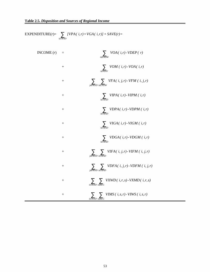
53

Table 2.5. Disposition and Sources of Regional Income

EXPENDITURE(r)= SAVE(r)+r)] i, ( VGA + r) i, ( [VPATRADi∑

ε

=

INCOME (r) = ∑ENDWiε

r) ( VDEP - r)i, ( VOA

+ ∑NSAViε

r) i, ( VOA - r) i, ( VOM

+ ∑∑ENDWiPRODj

εε

r) j, i, ( VFM - r) j, i, ( VFA

+ ∑TRADiε

r) i, ( VIPM - r) i, ( VIPA

+ ∑TRADiε

r) i, ( VDPM - r) i, ( VDPA

+ ∑TRADiε

r) i, ( VIGM - r) i, ( VIGA

+ ∑TRADiε

r) i, ( VDGM - r) i, ( VDGA

+ ∑∑TRADiPRODj

εε

r) j, i, ( VIFM - r) j, i, ( VIFA

+ ∑∑TRADiPRODj

εε

r) j, i, ( VDFM - r) j, i, ( VDFA

+ ∑∑REGsTRADi

εε

s)r, i, ( VXMD - s)r, i, ( VXWD

+ ∑∑REGsTRADi

εε

r) s,i, ( VIWS - r) s,i, ( VIMS

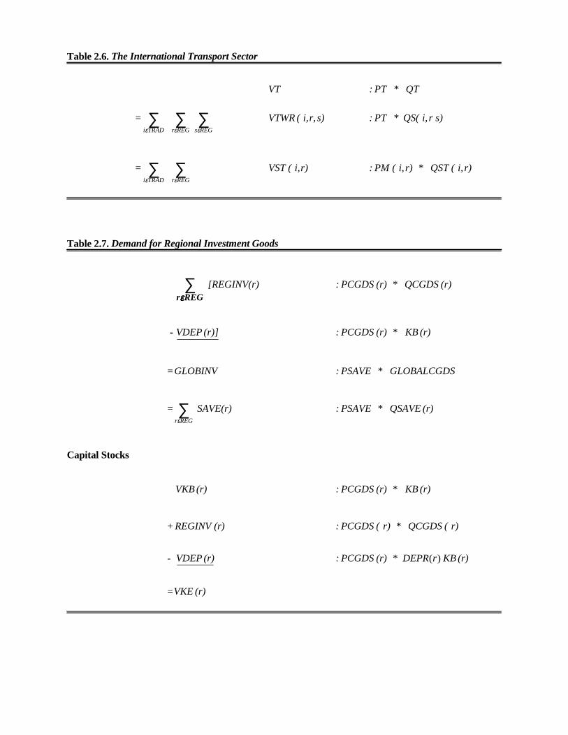
Table 2.6. The International Transport Sector

VT QT* PT :

∑∑∑REGsREGrTRADi

=εεε

s)r,i, ( VTWR s)r i, QS(* PT :

∑∑REGrTRADi

=εε

r)i, ( VST r) i, ( QST* r) i, ( PM :

Table 2.7. Demand for Regional Investment Goods

∑REGrεεεε

[REGINV(r) (r) QCGDS* (r) PCGDS :

- (r)] VDEP (r) KB* (r) PCGDS :

=GLOBINV GLOBALCGDS* PSAVE :

= ∑REGrε

SAVE(r) (r) QSAVE* PSAVE :

Capital Stocks

(r) VKB (r) KB* (r) PCGDS :

+ (r) REGINV r) ( QCGDS* r) ( PCGDS :

- (r) VDEP (r) KB rDEPR* (r) PCGDS : )(

= (r) VKE

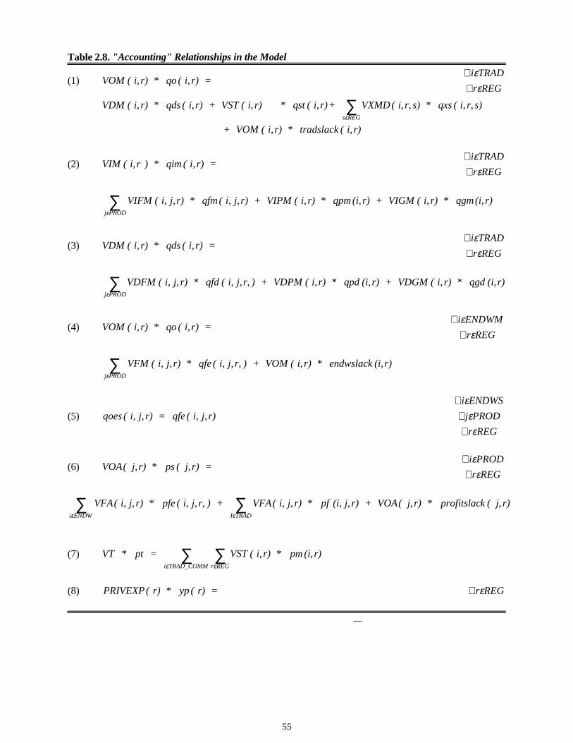
55

Table 2.8. "Accounting" Relationships in the Model

(1) = r) i, ( qo* r) i, ( VOMREGr

TRADi

εε

∀∀

r) i, ( tradslack* r) i, ( VOM +

s)r, i, ( qxs* s)r, i, ( VXMD +r) i, ( qst* r) i, ( VST + r) i, ( qds* r) i, ( VDMREGs∑ε

(2) = r) i, ( qim* ) r i, ( VIMREGr

TRADi

εε

∀∀

r) (i, qgm* r) i, ( VIGM + r) (i, qpm* r) i, ( VIPM + r) j, i, ( qfm* r) j, i, ( VIFMPRODj∑

ε

(3) = r) i, ( qds* r) i, ( VDMREGr

TRADi

εε

∀∀

r) (i, qgd* r) i, ( VDGM + r) (i, qpd* r) i, ( VDPM + )r, j, i, ( qfd* r) j, i, ( VDFMPRODj∑

ε

(4) = r) i, ( qo* r) i, ( VOMREGr

ENDWMi

εε∀

∀

r) (i, endwslack* r) i, ( VOM + )r, j, i, ( qfe* r) j, i, ( VFMPRODj∑

ε

(5) r) j, i, ( qfe = r) j, i, ( qoes

REGr

PRODj

ENDWSi

εε

ε

∀∀

∀

(6) = r) j, ( ps* r) j, ( VOAREGr

PRODi

εε

∀∀

r) j, ( kprofitslac* r) j, ( VOA + r) j, (i, pf* r) j, i, ( VFA + )r, j, i, ( pfe* r) j, i, ( VFATRADIENDWi∑∑

εε

(7) r) (i, pm* r) i, ( VST = pt* VTREGrTRAD_COMMi∑∑εε

(8) = r) ( yp* r) ( PRIVEXP REGrε∀

∑

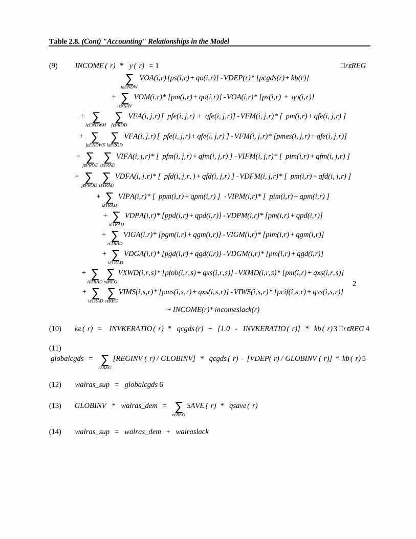
Table 2.8. (Cont) "Accounting" Relationships in the Model

(9) = r) (y * r) ( INCOME 1 REGrε∀

k(r)incomeslac* INCOME(r) +

r)]s,qxs(i, + r)s,[pcif(i,* r)s,VIWS(i, -r)] s,qxs(i, + r)s,[pms(i,* r)s,VIMS(i, +

s)]r,qxs(i, + r)[pm(i,* s)r,VXMD(i, -s)] r,qxs(i, + s)r,[pfob(i,* s)r,VXWD(i, +

r)]qgd(i, + r)[pm(i,* r)VDGM(i, -r)] qgd(i, + r)[pgd(i,* r)VDGA(i, +

r)]qgm(i, + r)[pim(i,* r)VIGM(i, -r)] qgm(i, + r)[pgm(i,* r)VIGA(i, +

r)]qpd(i, + r)[pm(i,* r)VDPM(i, -r)] qpd(i, + r)[ppd(i,* r)VDPA(i, +

] r)qpm(i, + r)pim(i, [* r)VIPM(i, -] r)qpm(i, + r)ppm(i, [* r)VIPA(i, +

] r)j,qfd(i, + r)pm(i, [* r)j,VDFM(i, -] r)j,qfd(i, + )r,j,pfd(i, [* r)j,VDFA(i, +

] r)j,qfm(i, + r)pim(i, [* r)j,VIFM(i, -] r)j,qfm(i, + r)j,pfm(i, [* r)j,VIFA(i, +

r)]j,qfe(i, + r)j,[pmes(i,* r)j,VFM(i, -] r)j,qfe(i, + r)j,pfe(i, [ r)j,VFA(i, +

] r)j,qfe(i, + r)pm(i, [* r)j,VFM(i, -r)] j,qfe(i, + r)j,pfe(i, [ r)j,VFA(i, +

r)]qo(i, + r)[ps(i,* r)VOA(i, -r)] qo(i, + r)[pm(i,* r)VOM(i, +

kb(r)] + [pcgds(r)* VDEP(r) -r)] qo(i, + r)[ps(i, r)VOA(i,

REGsTRADi

REGsTRADi

TRADi

TRADi

TRADi

TRADi

TRADiPRODj

TRADiPRODj

PRODiENDWSj

PRODjENDWMi

NSAVi

ENDWi

∑∑∑∑∑∑∑

∑

∑∑

∑∑

∑∑

∑∑∑∑

εε

εε

ε

ε

ε

ε

εε

εε

εε

εε

ε

ε

2

(10) r) ( kb* r)] ( INVKERATIO - [1.0 + (r) qcgds* r) ( INVKERATIO = r) ( ke 3 REGrε∀ 4

(11)r) ( kb* r)] ( GLOBINV / r) [VDEP( - r) ( qcgds* GLOBINV] / r) ( [REGINV = globalcgds

REGr∑ε

5

(12) globalcgds = walras_sup 6

(13) r) ( qsave* r) ( SAVE = _dem* walras GLOBINVREGr∑ε

(14) ack walrasl+ dem walras_= walras_sup

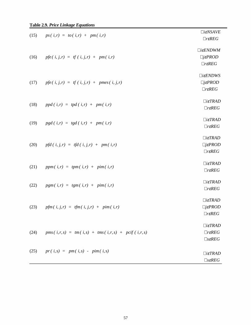
57

Table 2.9. Price Linkage Equations

(15) r) i, ( pm + r) i, ( to = r) i, ( psREGr

NSAVEi

εε

∀∀

(16) r) i, ( pm + r) j, i, ( tf = r) j, i, ( pfe

REGr

PRODj

ENDWMi

εε

ε

∀∀

∀

(17) r) j, i, ( pmes + r) j, i, ( tf = r) j, i, ( pfe

REGr

PRODj

ENDWSi

εε

ε

∀∀

∀

(18) r) i, ( pm + r) i, ( tpd = r) i, ( ppdREGr

TRADi

εε

∀∀

(19) r) i, ( pm + r) i, ( tgd = r) i, ( pgdREGr

TRADi

εε

∀∀

(20) r) i, ( pm + r) j, i, ( tfd = r) j, i, ( pfd

REGr

PRODj

TRADi

εεε

∀∀∀

(21) r) i, ( pim + r) i, ( tpm = r) i, ( ppmREGr

TRADi

εε

∀∀

(22) r) i, ( pim + r) i, ( tgm = r) i, ( pgmREGr

TRADi

εε

∀∀

(23) r) i, ( pim + r) j, i, ( tfm = r) j, i, ( pfm

REGr

PRODj

TRADi

εεε

∀∀∀

(24) s)r, i, ( pcif + s)r, i, ( tms + s)i, ( tm = s)r, i, ( pms

REGs

REGr

TRADi

εε

ε

∀∀∀

(25) s)i, ( pim - s)i, ( pm = s)i, ( pr

REGs

TRADi

εε

∀∀

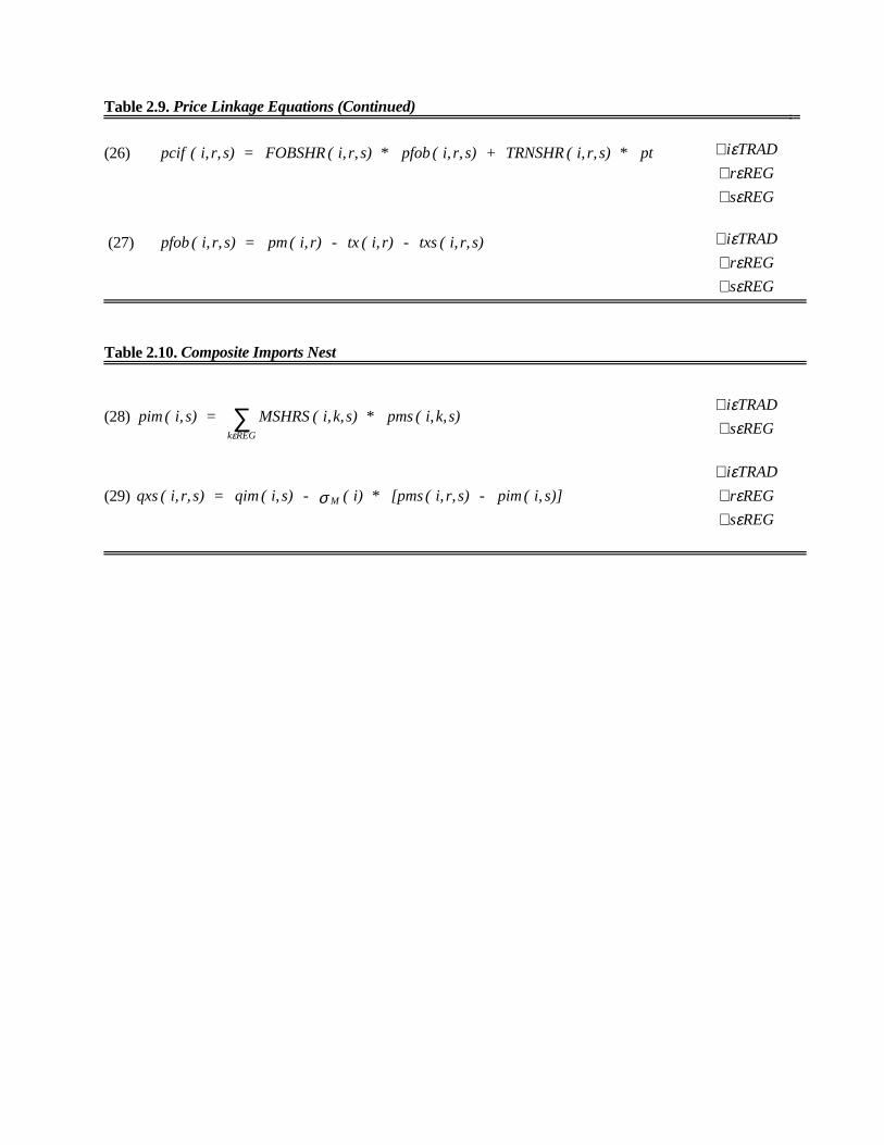
Table 2.9. Price Linkage Equations (Continued)

(26) pt* s)r, i, ( TRNSHR + s)r, i, ( pfob* s)r, i, ( FOBSHR = s)r, i, ( pcif

REGs

REGr

TRADi

εε

ε

∀∀∀

(27) s)r, i, ( txs - r) i, ( tx - r) i, ( pm = s)r, i, ( pfob

REGs

REGr

TRADi

εε

ε

∀∀∀

Table 2.10. Composite Imports Nest

(28) s)k, i, ( pms* s)k, i, ( MSHRS = s)i, ( pimREGk∑ε REGs

TRADi

εε

∀∀

(29) s)]i, ( pim - s)r, i, ( [pms* i) ( - s)i, ( qim = s)r, i, ( qxs MσREGs

REGr

TRADi

εε

ε

∀∀∀

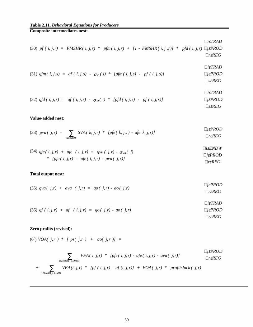
59

Table 2.11. Behavioral Equations for ProducersComposite intermediates nest:

(30) r) j, i, ( pfd* r)] j , i, ( FMSHR - [1 + r) j, i, ( pfm* r) j, i, ( FMSHR = r) j, i, ( pf

REGr

PRODj

TRADi

εεε

∀∀∀

(31) s)]j, i, ( pf - s)j, i, ( [pfm* i) ( - s)j, i, ( qf = s)j, i, ( qfm DσREGs

PRODj

TRADi

εεε

∀∀∀

(32) s)]j, i, ( pf - s)j, i, ( [pfd* i) ( - s)j, i, ( qf = s)j, i, ( qfd DσREGs

PRODj

TRADi

εεε

∀∀∀

Value-added nest:

(33) r)] j, k, afe - r) j, k, ( [pfe* r) j, k, ( SVA = r) j, ( pvaENDWk∑

ε REGr

PRODj

εε

∀∀

(34)

r)] j, ( pva - r) j, i, ( afe - r) j, i, ( [pfe*

j) ( - r) j, ( qva = r) j, i, ( afe + r) j, i, ( qfe VAσ

REGr

PRODj

ENDWi

εεε

∀∀∀

Total output nest:

(35) r) j, ( ao - r) j, ( qo = r) j, ( ava + r) j, ( qvaREGr

PRODj

εε

∀∀

(36) r) j, ( ao - r) j, ( qo = r) j, i, ( af + r) j, i, ( qf

REGr

PRODj

TRADi

εεε

∀∀∀

Zero profits (revised):

(6´) =)] r j, ao( + ) r j, ps( [* ) r j, VOA(

r) j, ( kprofitslac* r) j, ( VOA +r)] j, (i, af - r) j, i, ( [pf* r) j, (i, VFA +

r)] j, ( ava - r) j,i, ( afe - r) j, i, ( [pfe* r) j, i, ( VFA

TRAD_COMMi

ENDW_COMMi

∑

∑

ε

εREGr

PRODj

εε

∀∀

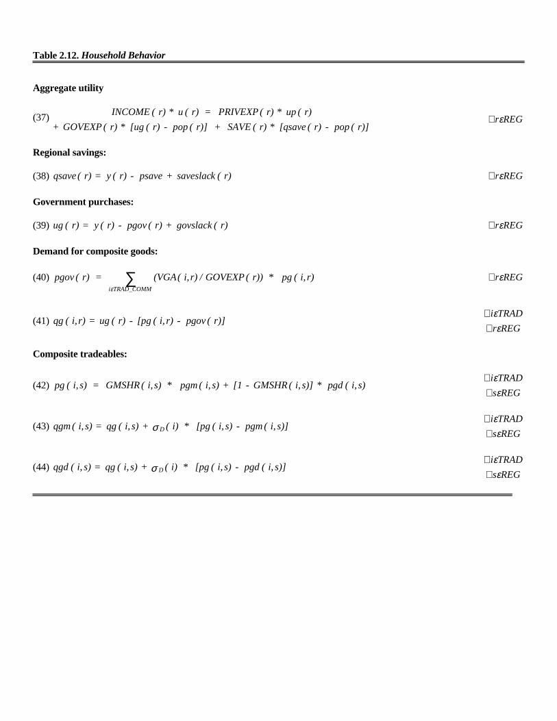
Table 2.12. Household Behavior

Aggregate utility

(37) r)] ( pop - r) ( [qsave* r) ( SAVE+r)] ( pop - r) ( [ug* r) ( GOVEXP +

r) ( up* r) ( PRIVEXP = r) (u * r) ( INCOMEREGrε∀

Regional savings:

(38) r) ( k saveslac+ psave - r) (y = r) ( qsave REGrε∀

Government purchases:

(39) r) ( govslack + r) ( pgov - r) (y = r) ( ug REGrε∀

Demand for composite goods:

(40) r) i, ( pg* r)) ( GOVEXP / r) i, ( (VGA = r) ( pgovTRAD_COMMi

∑ε

REGrε∀

(41) r)] ( pgov - r) i, ( [pg - r) ( ug = r) i, ( qgREGr

TRADi

εε

∀∀

Composite tradeables:

(42) s)i, ( pgd* s)] i, ( GMSHR - [1 + s)i, ( pgm* s)i, ( GMSHR = s)i, ( pgREGs

TRADi

εε

∀∀

(43) s)]i, ( pgm - s)i, ( [pg* i) ( + s)i, ( qg = s)i, ( qgm DσREGs

TRADi

εε

∀∀

(44) s)]i, ( pgd - s)i, ( [pg* i) ( + s)i, ( qg = s)i, ( qgd DσREGs

TRADi

εε

∀∀

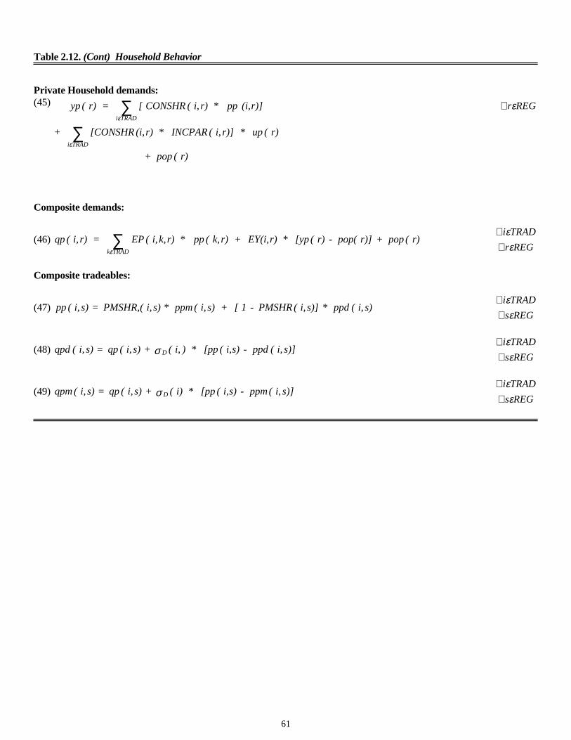
61

Table 2.12. (Cont) Household Behavior

Private Household demands:(45)

r) ( pop +

r) ( up* r)] i, ( INCPAR* r) (i, [CONSHR +

r)](i, pp* r) i, ( CONSHR [ = r) ( yp

TRADi

TRADi

∑∑

ε

ε

REGrε∀

Composite demands:

(46) r) ( pop +r)] pop( - r) ( [yp* r) EY(i, + r) k, ( pp* r) k, i, ( EP = r) i, ( qpTRADk∑

ε REGr

TRADi

εε

∀∀

Composite tradeables:

(47) s)i, ( ppd* s)] i, ( PMSHR - 1 [ + s)i, ( ppm* s)i, ( PMSHR, = s)i, ( ppREGs

TRADi

εε

∀∀

(48) s)]i, ( ppd - s)i, ( [pp* )i, ( + s)i, ( qp = s)i, ( qpd DσREGs

TRADi

εε

∀∀

(49) s)]i, ( ppm - s)i, ( [pp* i) ( + s)i, ( qp = s)i, ( qpm DσREGs

TRADi

εε

∀∀

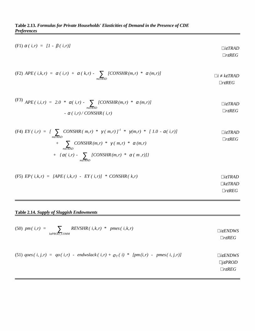
Table 2.13. Formulas for Private Households' Elasticities of Demand in the Presence of CDEPreferences

(F1) r)] i, ( - [1 = r) i, ( βα

REGr

TRADi

εε

∀∀

(F2) r)] (m, * r) (m, [CONSHR - r) k, ( + r) i, ( = r) k, i, ( APETRADm

αααε∑

REGr

TRADki

εε

∀≠∀

(F3)

r) i, ( CONSHR / r) i, ( -

r)] (m, * r) (m, [CONSHR - r) i, (* 2.0 = r) i, i, ( APETRADm

α

ααε∑

REGr

TRADi

εε

∀∀

(F4)

r)]} ,m ( * r) (m, [CONSHR - r) i, ({ +

r) (m, * r) m, ( * r) (m, CONSHR +

r)] i, ( - 1.0 [* r)(m,* ]r) m, ( * r) m, ( CONSHR[ = r) i, ( EY

TRADm

TRADm

-1

TRADm

αα

αγ

αγγ

ε

ε

ε

∑∑

∑REGr

TRADi

εε

∀∀

(F5) r)k, ( CONSHR* r)] i, ( EY - r) k, i, ( [APE = r) k, i, ( EP

REGr

TRADk

TRADi

εεε

∀∀∀

Table 2.14. Supply of Sluggish Endowments

(50) r) k, i, ( pmes* r) k, i, ( REVSHR = r) i, ( pmPROD_COMMk

∑ε

REGr

ENDWSi

εε

∀∀

(51) r)] j, i, ( pmes - r) (i, [pm* i) ( + r) i, ( endwslack - r) i, ( qo = r) j, i, ( qoes Tσ

REGr

PRODj

ENDWSi

εε

ε

∀∀

∀

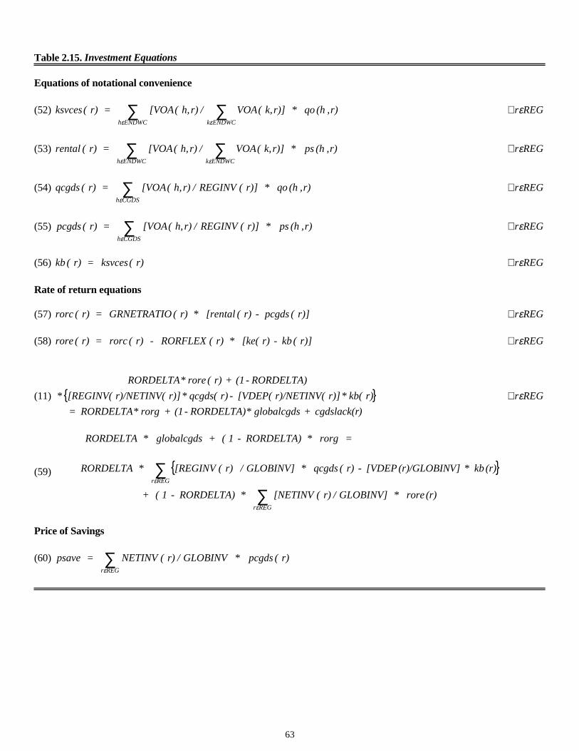
63

Table 2.15. Investment Equations

Equations of notational convenience

(52) r) ,(h qo* r)] k, ( VOA / r) h, ( [VOA = r) ( ksvcesENDWCkENDWCh∑∑

εε

REGrε∀

(53) r) ,(h ps* r)] k, ( VOA / r) h, ( [VOA = r) ( rentalENDWCkENDWCh∑∑

εε

REGrε∀

(54) r) ,(h qo* r)] ( REGINV / r) h, ( [VOA = r) ( qcgdsCGDSh∑

ε

REGrε∀

(55) r) ,(h ps* r)] ( REGINV / r) h, ( [VOA = r) ( pcgdsCGDSh∑

ε

REGrε∀

(56) r) ( ksvces = r) ( kb REGrε∀

Rate of return equations

(57) r)] ( pcgds - r) ( [rental* r) ( GRNETRATIO = r) ( rorc REGrε∀

(58) r)] ( kb - r) [ke(* r) ( RORFLEX - r) ( rorc = r) ( rore REGrε∀

(11) { })cgdslack(r + globalcgds* RORDELTA) - (1 + rorg* RORDELTA =

r) kb(* r)] r)/NETINV( [VDEP( -r) qcgds(* r)] r)/NETINV( [REGINV(*

RORDELTA) - (1 + r) ( rore* RORDELTA

REGrε∀

= rorg* RORDELTA) - 1 ( + globalcgds* RORDELTA

(59) { }

(r) rore* GLOBINV] / r) ( [NETINV* RORDELTA) - 1 ( +

(r) kb* V] (r)/GLOBIN [VDEP - r) ( qcgds* GLOBINV] / r) ( [REGINV* RORDELTA

REGr

REGr

∑∑

ε

ε

Price of Savings

(60) r) ( pcgds* GLOBINV / r) ( NETINV = psaveREGr∑ε

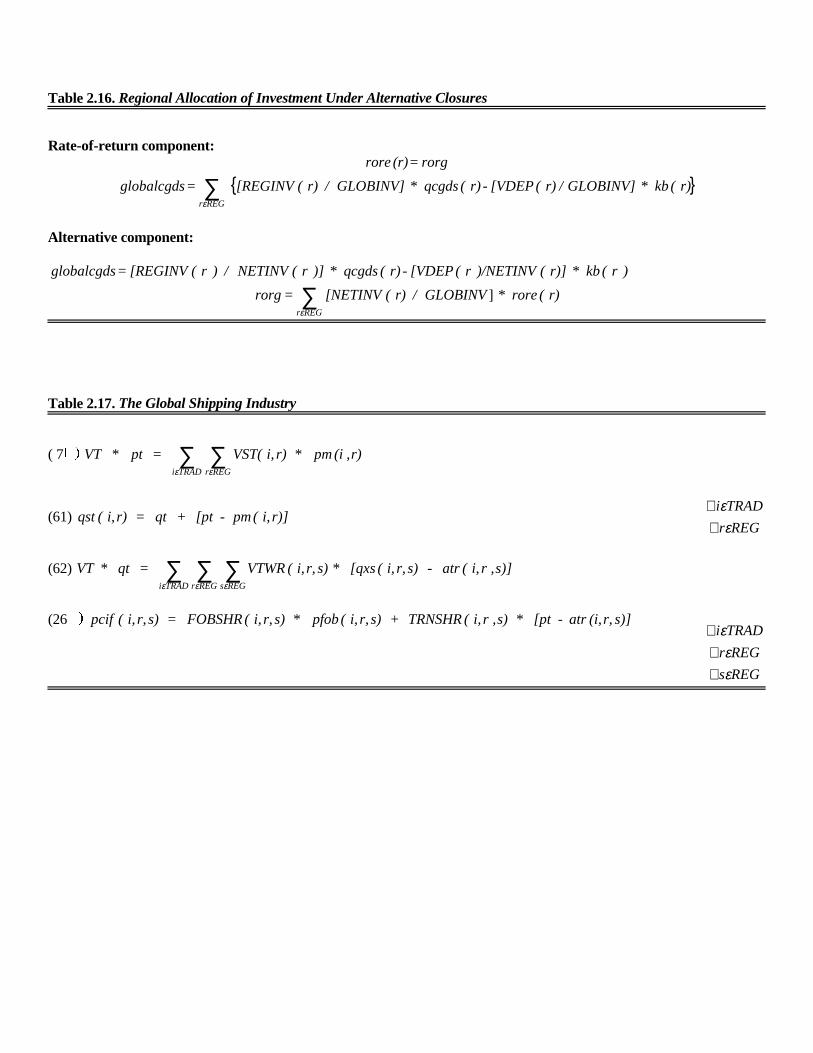
Table 2.16. Regional Allocation of Investment Under Alternative Closures

Rate-of-return component:rorg = (r) rore

{ }r) ( kb* GLOBINV] / r) ( [VDEP - r) ( qcgds* GLOBINV] / r) ( [REGINV = globalcgdsREGr∑ε

Alternative component:

) r ( kb* r)] ( )/NETINV r ( [VDEP - r) ( qcgds* )] r ( NETINV / ) r ( [REGINV = globalcgds

r) ( rore* GLOBINV / r) ( [NETINV = rorgREGr

]∑ε

Table 2.17. The Global Shipping Industry

( 7B! r) ,(i pm* r) i, VST( = pt* VTREGrTRADi∑∑εε

(61) r)] i, ( pm - [pt + qt = r) i, ( qstREGr

TRADi

εε

∀∀

(62) s)] ,r i, ( atr - s)r, i, ( [qxs* s)r, i, ( VTWR = qt* VTREGsREGrTRADi∑∑∑εεε

(26B! s)]r, (i, atr - [pt* s) ,r i, ( TRNSHR + s)r, i, ( pfob* s)r, i, ( FOBSHR = s)r, i, ( pcif

REGs

REGr

TRADi

εε

ε

∀∀∀

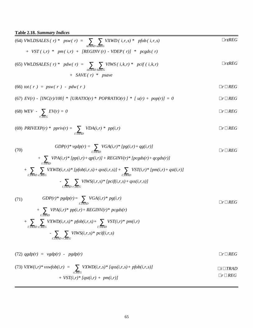
65

Table 2.18. Summary Indices

(64)

r) ( pcgds* r)] ( VDEP - (r) [REGINV + r) i, ( pm* r) i, ( VST +

s)r, i, ( pfob* s)r, i, ( VXWD = r) ( psw* r) ( VWLDSALESREGsTRADi∑∑εε

REGrε∀

(65)

psave* r) ( SAVE+

r) k, i, ( pcif* r) k, i, ( VIWS = r) ( pdw* r) ( VWLDSALESREGkTRADi∑∑εε

REGrε∀

(66) ) r ( pdw - ) r ( psw = ) r ( tot REGr ∈∀

(67) 0 =pop(r)] + u(r) [* ] )POPRATIO(r* [URATIO(r)* 0] [INC(r)/10 - EV(r) REGr ∈∀

(68) 0 = EV(r) - WEVREGr∑∈

REGr ∈∀

(69) r)pp(i,* r)VDA(i, = ppriv(r)* PRIVEXP(r)TRADi∑

∈

REGr ∈∀

(70)

s)]r,qxs(i,+s)r,[pcif(i,*s)r,VIWS(i,-

r)]qst(i,+r)[pm(i,*r)VST(i,+s)]r,qxs(i, + s)r,[pfob(i,*s)r,VXWD(i,+

qcgds(r)]+[pcgds(r)*REGINV(r)+r)]qp(i,+r)[pp(i,*r)VPA(i,+

r)]qg(i,+r)[pg(i,*r)VGA(i,= vgdp(r)*GDP(r)

REGrTRADi

TRADiREGsTRADi

TRADi

TRADi

∑∑∑∑∑

∑∑

∈∈

∈∈∈

∈

∈ REGr ∈∀

(71)

s)r,pcif(i,*s)r,VIWS(i,-

r)pm(i,*r)VST(i,+s)r,pfob(i,*s)r,VXWD(i,+

pcgds(r)*REGINV(r)+r)pp(i,*r)VPA(i,+

r)pg(i,*r)VGA(i,=pgdp(r)*GDP(r)

REGrTRADi

TRADiREGsTRADi

TRADi

TRADi

∑∑∑∑∑

∑∑

∈∈

∈∈∈

∈

∈ REGr ∈∀

(72) pgdp(r) - vgdp(r) = qgdp(r) REGr ∈∀

(73)

r)]pm(i, + r)[qst(i,* r)VST(i, +

s)]r,pfob(i, + s)r,[qxs(i,* s)r,VXWD(i, = r)vxwfob(i,* r)VXW(i,REGs∑∈

REGr

TRADi

∈∀∈∀

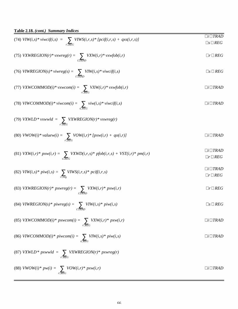
66

Table 2.18. (cont.) Summary Indices

(74) s)]r,qxs(i, + s)r,[pcif(i,* s)r,VIWS(i, = s)viwcif(i,* s)VIW(i,REGr∑∈ REGs

TRADi

∈∀∈∀

(75) r)vxwfob(i,* r)VXW(i, = vxwreg(r)* r)VXWREGION(TRADi∑

∈

REGr ∈∀

(76) s)viwcif(i,* s)VIW(i, = viwreg(s)* s)VIWREGION(TRADi∑

∈

REGs∈∀

(77) r)vxwfob(i,* r)VXW(i, = vxwcom(i)* i)VXWCOMMOD(REGr∑∈

TRADi ∈∀

(78) s)viwcif(i,* s)viw(i, = viwcom(i)* i)VIWCOMMOD(REGs∑∈

TRADi ∈∀

(79) vxwreg(r)* r)VXWREGION( = vxwwld* VXWLDREGr∑∈

(80) r)]qo(i, + r)[pxw(i,* r)VOW(i, = valuew(i)* VWOW(i)REGr∑∈

TRADi ∈∀

(81) r)pm(i,* r)VST(i, + s)r,pfob(i,* s)r,VXWD(i, = r)pxw(i,* r)VXW(i,REGs∑∈ REGr

TRADi

∈∀∈∀

(82) s)r,pcif(i,* s)r,VIWS(i, = s)piw(i,* s)VIW(i,regr

∑∈ REGr

TRADi

∈∀∈∀

(83) r)pxw(i,* r)VXW(i, = pxwreg(r)* r)VXWREGION(TRADi∑

∈

REGr ∈∀

(84) s)piw(i,* s)VIW(i, = piwreg(s)* s)VIWREGION(TRADi∑

∈

REGs∈∀

(85) r)pxw(i,* r)VXW(i, = pxwcom(i)* i)VXWCOMMOD(REGr∑∈

TRADi ∈∀

(86) s)piw(i,* s)VIW(i, = piwcom(i)* i)VIWCOMMOD(REGs∑∈

TRADi ∈∀

(87) pxwreg(r)* r)VXWREGION( = pxwwld* VXWLDREGr∑∈

(88) r)pxw(i,* r)VOW(i, = pw(i)* VWOW(i)REGr∑∈

TRADi ∈∀

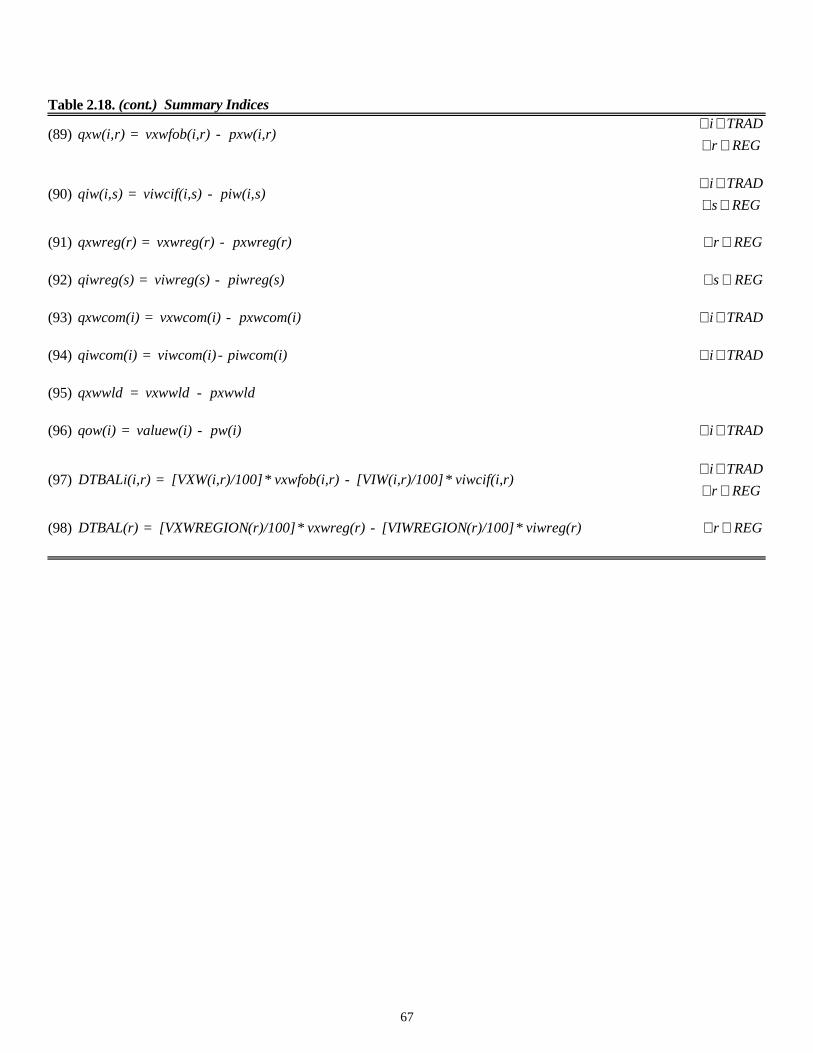
67

Table 2.18. (cont.) Summary Indices

(89) r)pxw(i, - r)vxwfob(i, = r)qxw(i,REGr

TRADi

∈∀∈∀

(90) s)piw(i, - s)viwcif(i, = s)qiw(i,REGs

TRADi

∈∀∈∀

(91) pxwreg(r) - vxwreg(r) = qxwreg(r) REGr ∈∀

(92) piwreg(s) - viwreg(s) = qiwreg(s) REGs∈∀

(93) pxwcom(i) - vxwcom(i) = qxwcom(i) TRADi ∈∀

(94) piwcom(i)- viwcom(i) = qiwcom(i) TRADi ∈∀

(95) pxwwld - vxwwld = qxwwld

(96) pw(i) - valuew(i) = qow(i) TRADi ∈∀

(97) r)viwcif(i,* r)/100] [VIW(i, - r)vxwfob(i,* r)/100] [VXW(i, = r)DTBALi(i,REGr

TRADi

∈∀∈∀

(98) viwreg(r)* (r)/100] [VIWREGION - vxwreg(r)* (r)/100] [VXWREGION = DTBAL(r) REGr ∈∀

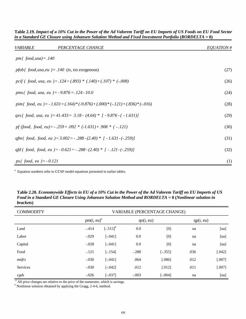
68

Table 2.19. Impact of a 10% Cut in the Power of the Ad Valorem Tariff on EU Imports of US Foods on EU Food Sectorin a Standard GE Closure using Johansen Solution Method and Fixed Investment Portfolio (RORDELTA = 0)

VARIABLE PERCENTAGE CHANGE EQUATION #

.140 = usa) food, ( pm

.140 = )eu usa, food, ( pfob (tx, txs exogenous) (27)

(-.008)* (.107) + (.140)* (.893) = .124 = )eu usa, food, ( pcif (26)

10.0 - .124 = 9.876- = )eu usa, food, ( pms (24)

(-.016)* (.836) + (-.121)* (.000) + (-9.876)* (.164) = 1.631- = )eu food, ( pim (28)

1.631)]- ( - 9.876- [* (4.64) - 3.18 = 41.433 = )eu usa, food, ( qxs (29)

.121)- (* .908 + (-1.631)* .092 = .259- = eu) food, (food, pf (30)

(-.259)] - 1.631- [* (2.40) - .288- = 3.002 = )eu food, food, ( qfm (31)

(-.259)] - .121- [* (2.40) - .288- = 0.621- = )eu food, food, ( qfd (32)

0.121- = )eu food, ( ps (1)

a Equation numbers refer to GTAP model equations presented in earlier tables.

Table 2.20. Economywide Effects in EU of a 10% Cut in the Power of the Ad Valorem Tariff on EU Imports of USFood in a Standard GE Closure Using Johansen Solution Method and RORDELTA = 0 (Nonlinear solution inbrackets)

COMMODITY VARIABLE (PERCENTAGE CHANGE)

pm(i, eu)a qo(i, eu) qp(i, eu)

Land -.414 [-.515]b 0.0 [0] na [na]

Labor -.029 [-.041] 0.0 [0] na [na]

Capital -.028 [-.041] 0.0 [0] na [na]

Food -.121 [-.154] -.288 [-.355] .036 [.042]

mnfrs -.030 [-.041] .064 [.086] .012 [.007]

Services -.030 [-.042] .012 [.012] .011 [.007]

cgds -.026 [-.037] -.003 [-.004] na [na]

a All price changes are relative to the price of the numeraire, which is savings.b Nonlinear solution obtained by applying the Gragg, 2-4-6, method.

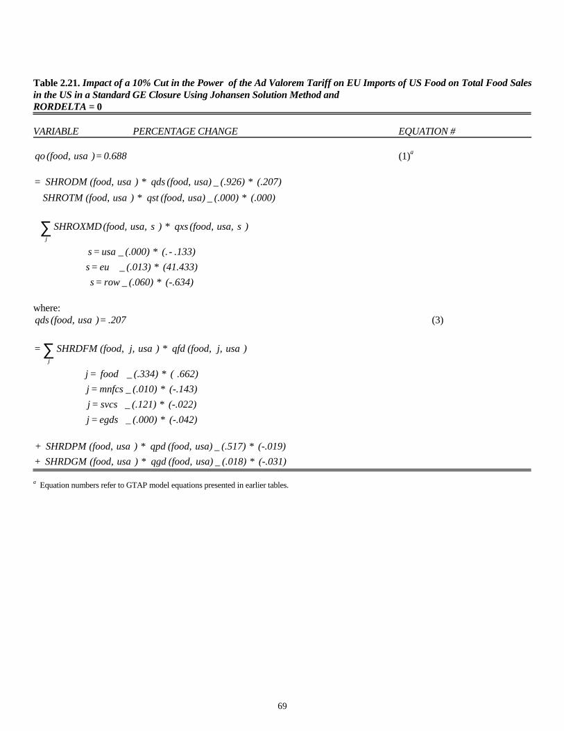
69

Table 2.21. Impact of a 10% Cut in the Power of the Ad Valorem Tariff on EU Imports of US Food on Total Food Salesin the US in a Standard GE Closure Using Johansen Solution Method andRORDELTA = 0

VARIABLE PERCENTAGE CHANGE EQUATION #

0.688 = ) usa (food, qo (1)a

(.207)* (.926) usa) (food, qds* ) usa (food, SHRODM= _

(.000)* (.000) usa) (food, qst* ) usa (food, SHROTM _

(-.634)* (.060) row = s

(41.433)* (.013) eu = s

.133)-(.* (.000) usa = s

) susa, (food, qxs* ) susa, (food, SHROXMD j

_

_

_

∑

where:.207 = ) usa (food, qds (3)

(-.042)* (.000) egds =j

(-.022)* (.121) svcs=j

(-.143)* (.010) mnfcs =j

.662) (* (.334) food =j

) usa j, (food, qfd* ) usa j, (food, SHRDFM =j

_

_

_

_

∑

(-.031)* (.018) usa) (food, qgd* ) usa (food, SHRDGM+

(-.019)* (.517) usa) (food, qpd* ) usa (food, SHRDPM+

_

_

a Equation numbers refer to GTAP model equations presented in earlier tables.

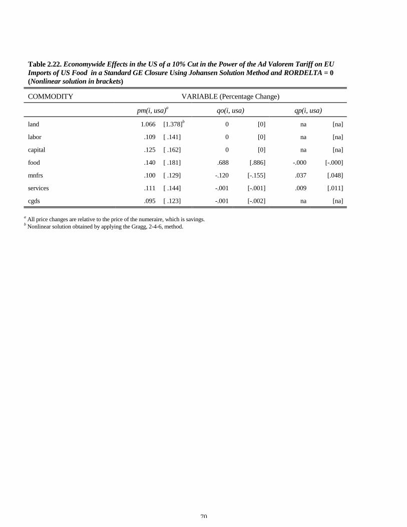
70

Table 2.22. Economywide Effects in the US of a 10% Cut in the Power of the Ad Valorem Tariff on EUImports of US Food in a Standard GE Closure Using Johansen Solution Method and RORDELTA = 0(Nonlinear solution in brackets)

COMMODITY VARIABLE (Percentage Change)

pm(i, usa)a qo(i, usa) qp(i, usa)

land 1.066 [1.378]b 0 [0] na [na]

labor .109 [ .141] 0 [0] na [na]

capital .125 [ .162] 0 [0] na [na]

food .140 [ .181] .688 [.886] -.000 [-.000]

mnfrs .100 [ .129] -.120 [-.155] .037 [.048]

services .111 [ .144] -.001 [-.001] .009 [.011]

cgds .095 [ .123] -.001 [-.002] na [na]

a All price changes are relative to the price of the numeraire, which is savings.b Nonlinear solution obtained by applying the Gragg, 2-4-6, method.

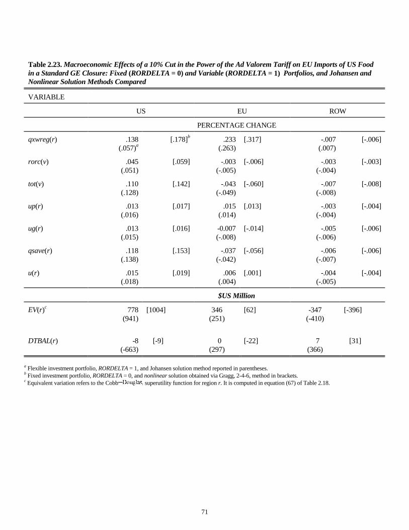
71

Table 2.23. Macroeconomic Effects of a 10% Cut in the Power of the Ad Valorem Tariff on EU Imports of US Foodin a Standard GE Closure: Fixed (RORDELTA = 0) and Variable (RORDELTA = 1) Portfolios, and Johansen andNonlinear Solution Methods Compared

VARIABLE

US EU ROW

PERCENTAGE CHANGE

qxwreg(r) .138(.057)a

[.178]b .233(.263)

[.317] -.007(.007)

[-.006]

rorc(v) .045(.051)

[.059] -.003(-.005)

[-.006] -.003(-.004)

[-.003]

tot(v) .110(.128)

[.142] -.043(-.049)

[-.060] -.007(-.008)

[-.008]

up(r) .013(.016)

[.017] .015(.014)

[.013] -.003(-.004)

[-.004]

ug(r) .013(.015)

[.016] -0.007(-.008)

[-.014] -.005(-.006)

[-.006]

qsave(r) .118(.138)

[.153] -.037(-.042)

[-.056] -.006(-.007)

[-.006]

u(r) .015(.018)

[.019] .006(.004)

[.001] -.004(-.005)

[-.004]

$US Million

EV(r)c 778(941)

[1004] 346(251)

[62] -347(-410)

[-396]

DTBAL(r) -8(-663)

[-9] 0(297)

[-22] 7(366)

[31]

a Flexible investment portfolio, RORDELTA = 1, and Johansen solution method reported in parentheses.b Fixed investment portfolio, RORDELTA = 0, and nonlinear solution obtained via Gragg, 2-4-6, method in brackets.c Equivalent variation refers to the Cobb�� superutility function for region r. It is computed in equation (67) of Table 2.18.

Documents

by Thomas W. Hertel and Marinos E. Tsigas I. … Models_Marco/Hertel and Tsigas (1997) Structure of...by Thomas W. Hertel and Marinos E. Tsigas ∗This is a draft of Chapter 2: "Structure