1World Bank, Development Research Group, email: sahmed20@worldbank.org, 2Department of Environmental Earth System Science and Woods Institute for the Environment, Stanford University, CA, 3Purdue University, Department of Agricultural Economics, 4World Bank, Development Research Group, Agriculture and Rural Development. This study has been prepared within the UNU-WIDER project on Development under Climate Change, directed by Channing Arndt. UNU-WIDER gratefully acknowledges the financial contributions to the project by the Finnish Ministry for Foreign Affairs and the Swedish International Development Cooperation Agency—Sida, and the financial contributions to the research programme by the governments of Denmark (Ministry of Foreign Affairs), and the United Kingdom (Department for International Development).

Working Paper No. 2011/91 Agriculture and Trade Opportunities for Tanzania Past Volatility and Future Climate Change Syud Amer Ahmed,1 Noah S. Diffenbaugh,2 Thomas W. Hertel,3 and William J. Martin4

December 2011

Abstract

Given global heterogeneity in climate-induced agricultural variability, Tanzania has the potential to substantially increase its maize exports to other countries. If global maize production is lower than usual due to supply shocks in major exporting regions, Tanzania may be able to export more maize at higher prices, even if it also experiences below-trend productivity. Diverse destinations for exports can allow for enhanced trading opportunities when negative supply shocks affect the partners’ usual import sources. Future climate predictions suggest that some of Tanzania’s trading partners will …/

Keywords: climate change, volatility, Tanzania, trade, export ban, agriculture

JELclassification: D58 F17 Q54

The World Institute for Development Economics Research (WIDER) was established by the United Nations University (UNU) as its first research and training centre and started work in Helsinki, Finland in 1985. The Institute undertakes applied research and policy analysis on structural changes affecting the developing and transitional economies, provides a forum for the advocacy of policies leading to robust, equitable and environmentally sustainable growth, and promotes capacity strengthening and training in the field of economic and social policy making. Work is carried out by staff researchers and visiting scholars in Helsinki and through networks of collaborating scholars and institutions around the world.

www.wider.unu.edu publications@wider.unu.edu

UNU World Institute for Development Economics Research (UNU-WIDER) Katajanokanlaituri 6 B, 00160 Helsinki, Finland Typescript prepared by Lisa Winkler at UNU-WIDER The views expressed in this publication are those of the author(s). Publication does not imply endorsement by the Institute or the United Nations University, nor by the programme/project sponsors, of any of the views expressed.

experience severe dry conditions that may reduce agricultural production in years when Tanzania is only mildly affected. Tanzania could thus export grain to countries as climate change increases the likelihood of severe precipitation deficits in other countries while simultaneously decreasing the likelihood of severe precipitation deficits in Tanzania. Trade restrictions, like export bans, prevent Tanzania from taking advantage of these opportunities, foregoing significant economic benefits.

Acknowledgement

The authors are grateful for helpful feedback from Madhur Gautam, Sergiy Zorya, two anonymous referees, and the participants of the 13th Annual Conference on Global Economic Analysis held in Penang, Malaysia in June 2010. The views and opinions expressed in this paper are solely those of the authors. This research was supported by the Trust Fund for Environmentally and Socially Sustainable Development. An earlier version of this study was released in the World Bank Policy Research Working Paper Series.

Figures and tables appear at the end of the paper.

1

1 Introduction

There is substantial evidence that the frequency and intensity of extreme climate events may change in the coming decades (Diffenbaugh et al. 2005; Easterling et al. 2000; IPCC 2007), with these changes being particularly important for agriculture (Lobell et al. 2008; White et al. 2006; Mendelsohn et al. 2007). Sub-Sahara African (SSA) countries, like Tanzania, are particularly sensitive to climate extremes due to their reliance on rain-fed subsistence agriculture. Schlenker and Lobell (2009) estimate that average maize productivity in SSA may decline by 22 percent by mid-century. These projected declines have severe development and poverty implications given that maize is the most important staple food in Eastern Africa and the most widely traded agricultural commodity (World Bank 2009).

However, there is considerable heterogeneity in the impacts of climate change across countries, and so international agricultural markets may allow for pooling of the risk posed by local (or national) climate extremes. Farmers in countries that are less severely affected by particular weather outcomes may be able to sell excess supply to meet the excess demand from consumers in the more severely affected regions.In the medium- to long-run, declines in agricultural production arising from climate change in some countries might be offset by increases in production in other regions.Open trade regimes have the potential to reduce domestic price volatility. For example, an open trade regime restricts the increase in food prices to the import parity price in the event of a drought (Dorosh et al. 2007), and open trade also bounds price declines at export parity in the event of a favorable productivity shock.

Despite the apparent benefits of greater openness to trade as a mechanism to reduce food supply variability and food price volatility, the trade policy response to climate volatility may in fact be one of greater international agricultural price insulation.Reilly et al. (1994) identify concerns about national food self-sufficiency as an argument used by countries to institute greater trade restrictions, with the restrictions becoming attractive mechanisms to maintain food supply objectives. Similarly, the food price crisis of 2007–08 saw several countries erect export restrictions to enhance domestic food availability. As Mitra and Josling (2009) discuss, these export restrictions often had the additional goal of reducing domestic price volatility—an important policy objective in many countries—despite their potentially limited efficacy.

Tanzania was one such country, instituting a crisis-induced export ban on maize (FAO 2009) that has only recently been lifted.The World Bank (2009) makes the case that, in addition to limiting crossborder trade1, it also has other impacts—in particular reducing producer prices and reducing potential output. This stands in sharp contrast to the underlying, sizable production potential in Tanzania, and the potential to supply neighboring countries that may experience structural food deficits (World Bank 2009). Therefore, it can be argued that the export ban has not only lowered exports, but has also led to slower agricultural growth, and lost opportunities for farmers and consumers.

1 Data from RATIN (2009) indicate that there is substantial informal cross-border trade.

2

Due to the potentially important role that trade policy can play in mitigating the effects of climate on production, the interaction of international trade with agricultural production shocks arising from climate change has been explored in the literature (e.g., Tobey et al. 1992; Reilly et al. 1994; Tsigas et al. 1997; Randhir and Hertel 2000). However, the aforementioned studies focus only on decadal scale, mean climate change, and do not consider the impact of changing climate volatility and the incidence and intensity of extreme events. Also, the scope of many of these studies is constrained by data limitations that prohibited analysis of individual African countries. Reimer and Li’s (2009) more recent examination of cereal and oilseeds trade finds that world trade volumes will need to increase if yield variability increases. However, this analysis is unable to examine the complex interaction of factor incomes and prices in determining how household level welfare—especially of poor households—may vary, as has been shown to be the case in the presence of international price shocks following trade liberalization (e.g., Hertel et al. 2004; Hertel and Winters 2006; Hertel et al. 2009) and in recent analyses of climate change and poverty (Ahmed et al. 2009, 2011).

Tanzania is a country where grain production variability may increase due to changing climate volatility (Ahmed et al. 2011). In this paper, we examine the sensitivity of prices and factor incomes in Tanzania due to climate volatility. Of particular interest are the potential inter-annual trading opportunities created by heterogeneous climate shocks, as well as the potential for trade to modulate the effects of climate-induced shocks on Tanzanian poverty.

In order to examine these potential trade effects, we first estimate the historical covariance of maize productivity shocks in Tanzania and her key trading partners. We then use an augmented version of the Global Trade Analysis Project (GTAP) global trade model and associated database to quantitatively examine the interaction between trade policy and the climate-induced maize production volatility, with emphasis on the resulting impacts on exports and poverty in Tanzania. We consider these impacts within the context of five historical casestudy years in which we apply the historical productivity shocks under two different trade regimes to examine the sensitivity of the economic impacts of climate shocks to export restrictions. Finally, we use a suite of global climate model simulations to quantify the potential for changes in precipitation extremes in Tanzania and in key trading partners as greenhouse gas concentrations increase over the course of the 21st century.

2 Tanzanian maize trade in the context of international production volatility

Tanzanian trade policy emphasizes integration into the regional and multi-lateral trading systems, as reflected in the National Trade Policy (United Republic of Tanzania 2003), which sets the goal of guiding the country from a supplyconstrained economy to one with competitive, export-led growth. Export growth has been credited with an important role in raising the national growth rate from 2 percent per annum in 1990–95 to 6 percent in 2000–03 (Integrated Framework 2005).The National Trade Policy, however, provides only a weak and superficial treatment of agriculture-enhancing policies, even though crop exports accounted for about 23 percent of total export value in 2001 (Dimaranan 2006). There also appears to be little coordination of trade, agriculture, and poverty reduction strategies, despite the importance of

3

sustaining export growth indicated in the National Strategy for Growth and Reduction of Poverty (United Republic of Tanzania2005).

Focusing on maize, Tanzania’s trade policies have a history of rapid changes and great uncertainty, as reviewed by Chapoto and Jayne (2010). For example, the government lifted a long-standing ban on maize exports around the same time that the East African Community was established (1999). However, in 2003, the Ministry of Agriculture and Food Security imposed an export ban on maize by withdrawing export permits already issued to traders and suspending the issuance of new permits. In 2006, this ban was lifted for a month, and then reimposed, before being lifted again in late 2010.

Table 1 reports data on maize production, imports, and exports by year (USDA 2011). These data show thatboth imports and exports tend to be very small as a share of domestic consumption and production. Exports are reported in nine of the 22 years considered in Table 1. By contrast, imports are recorded in 20 of the 22 years. Given that export bans have been in place for much of this period, it is hardly surprising that producers and marketing institutions have not pursued long run expansion of exports, assuming instead that production will be consumed domestically.

As Table 2 illustrates, the modest values of Tanzanian exports and imports of maize are concentrated on a small set of partners. Western Europe and the USA are the major trading partners in terms of both exports and imports. Tanzania trades very little with other African countries, with total exports to other SSA countries accounting for less than 22 percent of all maize exports and 25 percent of all maize imports. Among African countries, Uganda and Malawi are important sources of maize, supplying 15 percent of imported maize. These trade patterns reflect a number of factors, including: historical ties, logistical costs, Tanzania’s myriad trade agreements and preferences, the barriers that Tanzania places on its own imports and exports, as well as those barriers faced by its exports in other markets.

In principle, Tanzania should be affected by climate volatility in major grain exporting or importing countries since that volatility translates into maize production volatility, subsequently affecting the import price, the world price, and the demand for Tanzanian maize. Trade may thus allow Tanzania the opportunity to take advantage of international climate and production heterogeneity in any given year to either mitigate the impacts of a lower-than-usual yield or take advantage of a higher-than-usual yield. For example, if Tanzanian maize productivity is above trend in a year when a major global maize trader like the USA has below-trend productivity, Tanzania may be able to benefit by exporting more maize at higher world prices.

This point is best illustrated by Table 3 (column 1), describing the international correlations in maize production deviations from trend between 1971 and 2001 for Tanzania and the world’s major producing regions. These deviations from trend can be conceptualized as being attributable to idiosyncratic shocks—including, most importantly, weather. There is positive correlation in production deviations from trend for Tanzania and many regional neighbors –Uganda, Malawi, Zambia, the Rest of Eastern Africa, and the Rest of SSA. This reflects the fact that when Tanzania experiences a given climate outcome that damages agricultural production in a given year (e.g., a drought) countries that are geographically close to it are likely to have similar experiences. Conversely, if Tanzania experiences climate that is conducive to good

4

yields, and subsequently has aboveaverage maize production, then its near neighbors are likely to experience the same positive climate. In contrast there is low, or negative, correlation between Tanzania’s maize production volatility and the volatility in major maize traders like Argentina, the USA, and Western Europe.

In order to explore the potential for trade to buffer or intensify the effects of climatechange-induced grain production volatility, we select from our time series of production deviations from trends, five individual historical years in which Tanzania and/or her major trading partners experienced large deviations from their respective maize production trends. The historical testcase approach is motivated by the known importance of climate for grain production (e.g., Lobell et al. 2008), the anticipated damages to SSAn agriculture due to climate change (Schlenker and Lobell 2010), and the negative effects of grain productivity shocks on poverty in developing countries (Ahmed et al. 2009, 2011). Given this chain of influence linking climate, grains production and poverty, these casestudy years allow us to quantitatively test the potential for different trade regimes to moderate the impacts of climate change on poverty, within the context of known productivity shocks in Tanzania and key trading partners. Columns (2)–(6) of Table 3 report production deviations from trend in our five selected years over the 1971–2001 period.

Let us begin with the cases in which Tanzania experiences positive deviations from trend, as reported in columns (2) (1995) and (3) (1971) of Table 3. In 1995, Tanzania’s production was 19 percent above trend, while major exporters like the USA and Argentina had sub-par production (recall the negative correlation of these regions with Tanzanian maize deviations in column 1). Maize production was also below-trend in many Southern and East African countries. Uganda, one of Tanzania’s neighbors, also had substantially higher production that year. In contrast, Uganda had lowerthantrend production in 1971 when Tanzania had above trend yields.

In 1980, Tanzania’s production was close to trend (hence the column label: Tanzania 0), while Uganda—a major source of maize imports into Tanzania—experienced a large negative production shock. Globally, many major maize producers and exporters experienced below-trend production in that same year.In contrast, Tanzania had below average production in 1982 and 1983. In 1982, major maize exporters had aboveaverage production, putting downward pressure on prices. In contrast, in 1983, some of those major exporters had belowaverage production pushing up global maize prices to the advantage of smaller maize exporters that had good harvests in that year.

International maize trade in each of these scenarios could have had beneficial or detrimental impacts on Tanzania. However, an export ban on grains would have made it impossible for Tanzania to take advantage of higher world prices, especially in years like 1995 and 1971, when it had aboveaverage production while other African countries and major global traders had low production. Analysis of FAOSTAT maize trade shows that there were 14 years when Tanzania did not officially export any maize.2 In six of these 14 years—1976, 1977, 1981, 1986, 1996, and 1996—Tanzania had a positive maize production deviation from trend.In some of these cases,

2 1972–74, 1976, 1977, 1981–86, 1994–96.

5

the world price of maize was also above trend, suggesting that the country was missing an opportunity to take advantage of the higher commodity prices. While import restrictions in partner countries surely played a role in limiting Tanzania’s exports, Tanzania has had a range of different initiatives in place that have also contributed to low levels of exports.3 For example, in 1995, when Tanzania had higherthanusual maize production, the world price of maize was 38 percent above trend.4 However, there was an export ban in place which limited the country’s ability to capitalize on this market development. This was finally lifted at the end of 1996, allowing Tanzania to export at greaterthantrend world maize prices till 1998, after which maize prices dropped below-trend again. All of this suggests the need to systematically investigate the role of Tanzanian trade policy in the context of volatile grains production nationally, regionally, and globally.

3 Methodology

Tanzania’s response to the type of global maize production heterogeneity delineated in the five casestudy years must be understood through mechanisms that can control for the substantial year-to-year changes in the global economy, and the frequent changes in Tanzanian maize trade policy that have occurred over the 1971–2001 period. In order to understand the poverty implications of the Tanzania’s responses, the mechanism must also account for the changes in prices and factor incomes that will occur across multiple markets, and other general equilibrium (GE) effects. For example, the Tanzanian maize sector employs about 30 percent of agricultural labor, or 13 percent of all workers in the economy. Shocks that affect the demand for labor in the maize sector thus have implications for all industries. Since we are interested in the sensitivity of poverty changes to climate volatility under the different maize trade regimes, we also need to track the impact on non-farm earnings as well as the consumption of goods and services.These variables will be affected directly by the shocks to the maize sector. However, given the importance of maize in the economy, they will also be affected indirectly through changes in other commodity prices and on the changes in wages, all determined in general equilibrium.

A computable GE simulation approach is thus necessary, and we employ a modified version of the GTAP simulation model. In addition to allowing us to estimate the changes in consumer prices and earnings stemming from changes to agricultural productivity due to climate effects, this approach also allows us to examine the additional sensitivity of Tanzania’s economic responses to the historical maize production heterogeneity under alternative trade regimes, without including the additional uncertainties of a forecasting approach.

3 See Anderson and Valenzuela (2008), Chapoto and Jayne (2010), Morrissey and Leyaro (2007), and World Bank (2009) for detailed reviews.

4 World maize prices are obtained from the World Bank’s Development Prospect Group’s GEM database. The price series for maize is in constant 2000 USD/MT. The time series is de-trended with maize prices explained by a quadratic function of time. The world price percent deviations from trend are then estimated from the ratio of the estimated residuals to the predicted prices. The world maize price time series and the percent deviations from trend are available in the appendices of the World Bank working paper version.

6

3.1 Model description

We begin with the GTAP Database Version 6 (Dimaranan 2006) and use this with a modified version of the standard GTAP model (Hertel 1997). Maize is included in the GTAP database and model parameters as a component of the ‘coarse grains’ composite commodity group. In Tanzania, maize accounts for more than 78 percent of the total output of ‘coarse grains’ and more than 98 percent of ‘coarse grains’ trade. As such, we consider the market and production structure of the Tanzanian ‘coarse grains’ sector to be a reasonable approximation of the Tanzanian maize sector. The global database has the additional advantage of reconciling the global input-output and trade data from a range of sources, and benchmarking them to a single representative year; 2001 in our particular case. The reconciled data may thus not be perfectly consistent with other data sources for any specific variable (e.g., 2001 exports of a specific commodity between a pair of countries, measured at the tariff-line from COMTRADE). However, they provide the global consistency necessary for analytical modeling. Also, given that official African trade data are of varying quality and may not account for informal trade flows (RATIN 2009), the GTAP database has the advantage of being a globally consistent and balanced database.Additionally, the analysis in this paper focuses on the sensitivity of this ‘representative’ Tanzanian economy5 to a very specific set of stressors, where the comparability of the effects of the different realizations of the stressors (i.e., the climate shocks) will be maintained as long as the same benchmark representative dataset is used in every realization.

We retain the empirically robust assumptions of constant returns to scale and perfect competition, and introduce factor market segmentation, following the methodology of Keeney and Hertel (2005). This segmentation is particularly important in countries where poverty occurs in rural areas. Farm and non-farm mobility of factors are restricted by specifying a constant elasticity of transformation function which allows ‘transformation’ of farm employed labor and capital into non-farm uses and vice-versa. This allows for persistent wage differences between the farm and non-farm sectors, and is the foundation of the inter-sectoral distributional analysis. In order to parameterize these factor mobility functions we draw on the OECD’s (2001) survey of agricultural factor markets—the best available database of the necessary elasticities with the widest country coverage. However, given the uncertainty about the appropriate values of these parameters for Tanzania, we conduct a systematic sensitivity analysis with respect to these parameters. We assume a constant aggregate level of land, labor, and capital employment reflecting the belief that the aggregate employment of factors is unaffected by the climate shocks that are affecting grain production.

The model is adjusted to distinguish between land classes with different biophysical characteristics, following the approach of Hertel et al. (2009). This distinguishes land by agro-

5 The data for domestic production and consumption in Tanzania is based on a 1992 input-output table that has subsequently been updated to be consistent using 2001 macro-economic and trade data. While a more recent input-output for Tanzania would be preferable, this was the most recent data made available during the construction of the GTAP database, and has passed several consistency checks. The full details on the input-output contribution, the database construction process, and the consistency checks can be found in the documentation for Dimaranan (2006).

7

ecological zone (AEZ), based on the data of Lee et al. (2009) and Monfreda et al. (2009). The model is then calibrated such that simulations of estimated historical productivity volatility of coarse grains for the 1971–2001 period replicate observed historical price volatility, as described in Ahmed et al. (2011).

In the model, the impact of the production deviation shocks on trade will be driven by changes in relative prices between alternative suppliers.The percentage change in demand for imports of commodity i from a specific country r into a country s ( irsqxs ) is a function of the change in aggregate imports of the commodity into s ( isqim ), the percentage change in the domestic price of i imported from r into s ( irspms ), the composite import price of all i imported into s ( ispim ), and the rate of import augmenting technological change ( irsams ), which captures the impact of changes in trade facilitation on any particular trade flow. Equation (1) describes this function.

( )irs irs is i irs irs isqxs ams qim pms ams pimσ= − + − − − (1)

Increases in the aggregate import demand for i in s will encourage more exports from country r. We term this the expansion effect. However, it is moderated, or perhaps strengthened, by the substitution effect which hinges on the change in the price of i from the exporting country r relative to the change in the aggregate import price (a weighted average of prices from all sources) in the importing country s determines whether the importing country will source more of commodity i from country r.

The parameter iσ is the so-called Armington elasticity of substitution amongst imports of the same commodity across different sources and it governs the responsiveness of the substitution effect amongst exporters. This elasticity is estimated in Hertel et al. (2007), using the data and approach of Hummels (1999).The approach exploited cross-sectional variation in delivered prices, by conditioning on an exporter and commodity. The elasticity of substitution was then identified from variation over importers in delivered prices which arose from bilateral variation in advalorem trade costs.

In order to understand how climate shocks can affect household welfare and poverty, we use the household micro-simulation model from Ahmed et al. (2011).That approach involves augmenting the CGE simulation framework with the household model of Hertel et al. (2004), to estimate changes in income and consumption of households in the neighborhood of the poverty line. For poverty analysis, the utility of the household at the poverty line is then defined as the poverty level of utility. If an adverse climate shock pushes households’ utility below this level, they enter poverty. Conversely, if they are lifted above this level of utility, they are no longer in poverty.The framework uses the AIDADS system to represent consumer preferences, and is calibrated using Tanzania’s Household Budget Survey 2000/2001.6Households are stratified into seven groups based on earnings sources. The poverty line in Tanzania is taken to match the

6 The poverty model is fully documented in Ahmed et al. (2011), including parameter estimates for the AIDADS demand system used.

8

observed national poverty headcount ratio reported by the World Bank (2005). This in turn dictates the poverty level of utility in the initial equilibrium.

3.2 Experimental design

The patterns of historical production deviations from trend for each of the five case study years highlighted in the previous section—Scenarios 1995 and 1971 (‘Tanzania +’), Scenario 1980 (‘Tanzania 0’), and Scenarios 1982 and 1983 (‘Tanzania –’) are reproduced in the model via an appropriate combination of international productivity shocks.7 We then consider the impacts on trade and poverty in the context of a range of different trade scenarios to explore the interplay between trade regimes and the poverty impacts of climate shocks.8

In order to mimic the short-run/transient nature of these productivity shocks, these simulations are conducted under the assumption that agricultural land and capital are immobile across sectors. That is, farmers are limited in their ability to adapt to different climate outcomes. For example, they are able to mobilize labor in response to a climate shock and adjust harvesting dates, but are not able to bring new irrigation infrastructure online in response to a single climate outcome. The allocation of cropland to a given crop is also pre-determined in this short-run model closure.

The production deviations for the five case study years are simulated under two different trade regimes, as perturbations from the benchmark world economy. Conducting all simulations as perturbations from trend allows for comparability across trade regimes. The two trade regimes are:

• Regime 1 (Baseline): the trade regime prevailing in the 2001 world economy. • Regime 2 (Export restriction): as in Regime 1, but with Tanzania imposing an export

restriction on maize, preventing maize exports from rising above their 2001 levels.

As noted above, Tanzania introduced grains export bans in response to the 2007–08 food price crisis. Tanzania had also relaxed import restrictions on grains as a response to the food price crisis, thereby raising domestic prices; however, these policies are not considered here.9 Implementation of the export restriction is treated via a complementary slackness condition, with the 2001 benchmark year’s export level taken as the quota level of exports. When changes in economic conditions push Tanzania’s maize exports to increase, they are prevented from rising above the 2001 benchmark year’s level by means of an endogenous export tax instrument. Maize

7 To obtain the appropriate scale for the productivity shocks, we perform a pre-simulation in which output is exogenous and productivity endogenous.

8 The production deviations for Mozambique, Rest of SSA, Southern Africa, Zambia, and Zimbabwe are not implemented under any scenario. The magnitudes of their deviations from trends were too large for the model to converge on a solution. Production in these countries can thus be assumed to be at trend for any given year simulated.

9 Several studies have examined the effects of import restrictions for other Africa countries (e.g., Dorosh et al. 2007; Haggblade et al. 2008).

9

trade flows, however, are permitted to fall below 2001 benchmark year levels if economic conditions dictate a decline in maize exports.

Since producers may adjust their production behavior in anticipation of future export restrictions we carry out one additional set of steps prior to conducting our scenario simulations. For example, if producers anticipate a regime of export restrictions where prices may be low in years with high yield because they cannot export any excess supply, they may choose to move some resources out of production of maize, reducing its benchmark supply. This behavior is approximated by conducting stochastic simulations of historical production variability in Tanzania, under the baseline trade regime and under the export restricted trade regime, to estimate how maize production may adjust on average in these two regimes. Based on the average production adjustment, we estimate factortax equivalents that provide an equivalent production shift to provide new benchmark databases for use with Regime 1 and Regime 2.

Finally, it should be noted that maize production perturbations under all casestudy scenarios are based on the same 2001 benchmark year, adjusted for pre-shock producer expectations about trade regimes. They thus allow for comparison of the marginal effects of the international climate heterogeneity in the casestudy year and of the trade regime in place without introducing additional uncertainty by replicating the global economy in the case study years.

4 Analysis

4.1 Additional impact of export restriction

Table 4 describes the marginal changes in maize exports from Tanzania due to maize productivity shocks in the case study years under the baseline regime, and under the additional effect of the export restriction regime. Under the baseline, Tanzanian maize exports expand for all export destinations in scenarios 1995 and 1971, when the country experiences positive deviations from its production trend (columns 1 and 2). This is driven by the large declines in the domestic price of maize in Tanzania, reported in Table 5.In terms of Equation (1), the large decreases in Tanzanian maize prices relative to her competitors, dominate any reduction in aggregate import demand, thereby increasing maize exports from Tanzania for all countries.10

Tanzania’s maize exports more than double for some trading partners. The largest percent increase is for maize exports from Tanzania to Uganda in scenario baseline-1971. Given the very

10 Due to the importance of the value of the Armington elasticity, the value of the elasticity was varied between 50 percent more and less than its initial value in a systematic sensitivity analysis. The impact on the results is small. For example, the percent change in the price of maize is -23.03 percent in scenario baseline 1995 and -25.94 percent in the scenario export restriction 1995. The standard deviations of the percent point changes in maize price in the two simulations, where the systematic sensitivity analysis is conducted, is 0.95 and 0.05. So, if we were considering a single standard deviation, the maize price change is between -22.08 percent and -23.98 percent in scenario baseline 1995, and between -25.91 percent and -25.97 percent in the export restriction scenario 1995. The analyses are thus robust to this parameter value and are discussed in more detail in the appendices of the World Bank working paper version.

10

low initial value of Tanzanian maize exports to Uganda (US$0.02 million), this development is less striking.11

Nonetheless, the results in Table 4 illustrate the important role of diverse trade partners in mitigating potential food security crises in the wake of a major supply shock.In 1971, maize production in Uganda was more than 25 percentbelow-trend. Given that 95 percent of its maize is for domestic consumption, this represents a major maize supply contraction. The high maize demand in Uganda, coupled with the higher supply in Tanzania allows Tanzania to substantially increase its exports, alongside those of a few other select countries.

In 1980, Tanzania’s maize production was essentially on trend, such that domestic supplies were little changed by idiosyncratic events such as climate shocks. In scenario baseline 1980, the changes in Tanzanian maize markets are largely driven by factors in the importing country that affect aggregate import demand and price. For example, Uganda’s maize production is almost 30 percentbelow-trend in this year, and there is a resulting high demand for maize imports generally. Almost all the increase in Ugandan imports of Tanzanian maize is driven by this higher demand. Let us contrast this with the case of East Asia, where maize production is also below-trend, and aggregate maize import demand also increases. However, the aggregate import price of maize declines while Tanzania’s maize price rises. This leads East Asia to source its maize imports from countries that have experienced positive supply shocks and thus have lower prices, e.g., China.Overall however, Tanzanian maize exports would have expanded by almost 7 percent in this baseline 1980.

The case of scenario baseline 1982 is the converse of scenarios 1995 and 1971. In this case, Tanzanian maize production was 13 percentbelow-trend, pushing up domestic prices by more than 28 percent. The supply shocks in other countries were such that this supply price effect dominated the effects of the other import determinants in Equation (1) and Tanzanian exports are predicted to fall across the board.

The case of baseline 1983 is more complicated. Even though total Tanzanian maize exports in scenario baseline 1983 decrease by about 28 percent, Tanzania is able to increase its exports to some countries that experienced even more negative deviations in their production from trend. For example, Tanzanian exports of maize to the USA—increased by 5 percent. The USA accounts for 15 percent of Tanzania’s maize exports and experienced production 40 percentbelow-trend in the Scenario Baseline 1983. These results are driven by events in the USA. Since the USA is responsible for more than 41 percent of the global maize trade in the benchmark database, this has dramatic implications for the aggregate maize import price in all countries.Almost all countries experience declines in aggregate demand for maize imports. However, since a country’s decision to import Tanzanian maize depends on both the substitution

11 In the short-run, the level of trade expansion (or contraction) is limited substantially by the initial level of trade and trade-related infrastructure. Since Uganda imported very little maize from Tanzania in the benchmark database, even this strong growth results in a final level of exports which are only a half million US$ higher. Therefore, all the percent changes in export flows must thus be considered in the context of their initial export levels, and as short-run trade changes.

11

and the expansion effect in Equation (1), a key factor is the change in relative prices of maize from Tanzania versus other exporters. For example, in the case of Tanzanian maize exports to Latin America and the Caribbean—an extremely minor destination for Tanzanian maize exports in the benchmark database –the substitution effect is positive and dominates the demand effect, and Latin America increases its imports of Tanzanian maize.

Let us now turn to the impacts of the export restriction regime—reported in the second group of columns in Table 4 as well as the price effects reported in Table 5. In the years when production is above trend and an export restriction is in place, the maize price may drop below the price that would have prevailed if there was no restriction.This can be seen in column (3) of Table 5. In the case of the years with positive shocks to Tanzanian maize production (scenarios 1995 and 1971), the domestic price of maize falls even more under the export restriction. With the export restriction in place, no increases in exports are possible (columns 6 and 7 in Table 4). In the case of scenario 1982, when Tanzanian maize production was below-trend, and maize exports decreased for all countries (since the modeling of the restriction allows for decreases from 2001 benchmark flows).

When considering the poverty impacts of production deviations from trend due to climate under trade Regimes 1 and 2, we must account for the impacts on prices as well as factor incomes, since changes in prices will change the cost of living. Looking at columns (1)–(3) in Table 6, we can see that poverty decreases in the years that Tanzania has a positive production deviation from trend (Scenarios 1995 and 1971), with most of the poverty reduction due to reductions in the cost of living. In both years, the price of maize, which is almost completely used for domestic consumption, falls substantially, even though the prices of other commodities increase somewhat. Poor households are thus able to purchase more at lower prices, reflecting the cost of living improvement. Improvements in earnings also contributed to the poverty reduction. The higher demand for workers in expanding downstream sectors like other food and beverages, farm livestock, and processed livestock leads to improvements to factor returns.

Tanzania’s negative deviations from maize production trends in 1980, 1982, and 1983 indicate increases in poverty in the casestudy simulations. In the case of Scenario 1980, the cost of living effect served to reduce poverty by 2400 people, but was overwhelmed by the 5200 people impoverished by the earnings effect. In the cases of Scenarios 1982 and 1982, there were sharp increases in food prices arising from the negative production shocks to maize, leading to major increases in poverty through higher costs of living.

The presence of an export restriction (Regime 2) is found to be generally poverty-increasing. In the case of Scenarios 1995 and 1971 it dampens both improvements in the cost of living as well as the effects of greater earnings.For Scenarios 1980, 1982, and 1983, the presence of an export exacerbates the lower factor returns, and leads to higher values for the poverty-increasing earnings effects.

Aside from generally being poverty-increasing (or dampening poverty reduction), the export restriction also has distributional implications. In the four scenarios where the export restriction increased poverty (1995, 1971, 1980, and 1983), the poverty increases were among households that depended on agriculture as the primary source of income, relied on transfers, or had diverse

12

sources of income. In contrast, the export ban actually had the marginal effect of reducing poverty among households that were not involved in agriculture, or relied on wages as their main source of income. The export restriction generally depresses returns to factor incomes, especially in agriculture. At the same time, households that rely less on agriculture are less detrimentally affected by lower factor incomes. So, even though all households benefit from the lower prices that an export ban might induce, wageincome-based and non-agricultural income-based households have smaller losses in their incomes, and are relatively better off.

The results of these case study simulations under Regimes 1 and 2 highlight a number of important considerations:12

• Tanzania has the potential to substantially increase its maize exports to other countries, and not only when its production is above trend. If global maize production is lower than usual due to supply shocks in major exporters, Tanzania can export more maize at higher prices, even if it also experiences below-trend production.

• Diversified sources of imports can help mitigate the effects of a negative supply shock in a major source, e.g., the case of Uganda increasing imports in 1971.

• Conversely, having diverse destinations for exports can allow for substantial trade when negative supply shocks affect the partners’ usual sources, e.g., Tanzania increasing exports to Latin America and the Caribbean when US production was below-trend in Scenario 1983.

• Export bans can suppress maize prices, either by making price declines larger, or price increases less positive. However, they are an ineffective tool for altering the poverty impact of the underlying climate/productivity shocks, and come at the cost of significant reductions in exports, GDPand long run credibility as a supplier of agricultural products.

4.2 Resultsprojected changes in climate extremes in Tanzania and trading partners

Given the sensitivity of poverty outcomes in Tanzania to both national trade policies and productivity shocks in key trading partners, we seek to quantify the potential changes in countrylevel climate extremes as greenhouse gas concentrations rise in the 21st century. As demonstrated in the preceding case studies, trade can potentially reduce the negative poverty impacts associated with increasing occurrences of negative climate outcomes in Tanzania—particularly if trading partners do not experience concurrent negative climate outcomes. Alternatively, trade can increase the benefits of reduced occurrence of negative climate outcomes in Tanzania, if trading partners experience negative climate outcomes in years when Tanzania

12 The choice of the parameters for the constant elasticities of transformation that modulate the mobility of factors between agriculture and non-agriculture affect several GE mechanisms important for the results. So, systematic sensitivity analysis was conducted to vary the parameters between zero and double their benchmark values for the baseline and export restriction scenario 1995. Briefly, the standard deviations of the percent point changes in maize price in the two simulations, when the systematic sensitivity analysis is conducted, is 0.03 and 0.06. So, if we were considering a single standard deviation, the maize price change is between -22.98 percent and -23.08 percent in scenario baseline 1995, and between -25.88 percent and -26.00 percent in the export restriction scenario 1995. The analyses are thus robust to this parameter and are discussed in more detail in the World Bank working paper version’s appendices.

13

does not. Therefore, we are particularly interested in the co-occurrence of climate extremes in Tanzania and her key trading partners. In order to better understand those potential responses, we use a suite of climate model experiments to project 21st century changes in (i) the occurrence of extreme dry years in Tanzania and her key trading partners; (ii) how often Tanzania experiences a dry year in the same year that her key trading partners do not experience dry years; and (iii) how often each of Tanzania’s key trading partners experiences a dry year in the same year that Tanzania does not experience a dry year.

4.3 Models, scenarios, and climate analyses

We analyse climate model results from the coupled model intercomparison project (CMIP3) (Meehl et al. 2007). CMIP3 has archived results from multiple general circulation models (GCMs) developed at climate modeling centers around the world. The archive has been extensively analysed by the international community, and the multi-model output served as the backbone of much of the Working Group I contribution to the Fourth Assessment Report (‘AR4’) of Intergovernmental Panel on Climate Change (IPCC) (IPCC2007).

The CMIP3 archive contains GCM simulations of the pre-industrial period, the 20th century, and various scenarios of the 21st century, including a number of the 21st century ‘SRES scenarios’ produced by the IPCC in its Special Report on Emissions Scenarios (IPCC 2000). Varying numbers of models have archived varying subsets of results for these different simulations. Together, these various climate model simulations create an ‘ensemble of opportunity’ that has been used to analyse a wide variety of phenomena in the climate system, including detection and attribution of historical climate change (e.g.,Santer et al. 2009), the sensitivity of global mean temperature to elevated greenhouse forcing (e.g.,Knutti et al. 2008), the response of extreme events to global warming (e.g., Tebaldi et al. 2006; Knutson et al. 2008; Diffenbaugh and Scherer 2011), and the potential impacts of climate change on natural and human systems (e.g., Williams et al. 2007; Ahmed et al. 2009; Battisti and Naylor 2009; Loarie et al. 2009).

In the present study, we focus on the CMIP3 simulations that have been forced by the IPCC A1B scenario (IPCC 2000). The cumulative CO2 emissions and global mean temperature change are very similar in the IPCC illustrative scenario suite over the first half of the 21st century (Meehl et al. 2007). The A1B scenario falls near the middle of the illustrative suite in the second half of the 21st century, with global atmospheric carbon dioxide concentrations reaching between 600 and 800 parts per million (ppm) by the end of the 21st century, and global mean temperature warming by between 2 and 4 ˚C (Meehl et al. 2007). For our analyses, we select ‘run 1’ from each of the 22 climate models that archived surface temperature and precipitation data for the A1B 21st century scenario.

Given the importance of adequate precipitation for maize production in Tanzania and the world (e.g., Ahmed et al. 2011; Lobell et al. 2008), we focus our analyses on the occurrence of dry years in Tanzania and key (or potential) trading partners during the 20th and 21st century CMIP3 simulations. For the purposes of this study, we take a dry year to be any year in which the annual precipitation is equal to or less than the historical 1-in-10-year dry event. We take the historical period to be 1951–2000, meaning that for each trading partner, the 1-in-10-year dry event is the 5th driest year in that partner during the 1951–2000 period, and a dry year is any year in which

14

the annual precipitation is less than or equal to the precipitation value of the 5th driest year of the 1951–2000 period.13

We use the CMIP3 climate model experiments to quantify the likelihood of different trading partners experiencing dry years, including the likelihood that these dry years co-occur in Tanzania and the trading partners. To do so, we first calculate the annual precipitation in each partnercountry in each year from 1951 through 2000. We then calculate the magnitude of the 1-in-10-year dry event for each trading partner for the 1951–2000 period, which we may call the ‘dry year threshold’.

Having obtained the dry year threshold for each partner for the 1951–2000 period, we calculate three metrics of dry year occurrence in each decade of the CMIP3 A1B 21st century projections:

• We calculate the number of dry years in Tanzania and her key trading partners. This metric indicates the likelihood that each trading partner will experience adverse climate conditions for grains production. For each trading partner, we report the number of dry years in each decade of the 21st century.

• We calculate how often Tanzania experiences a dry year in the same year that her key trading partners do not experience dry years. This metric indicates the likelihood that Tanzania’s trading partners will experience non-adverse climate conditions in the same year that Tanzania experiences adverse conditions, therefore offering the potential for Tanzania to ameliorate adverse conditions in Tanzania through trade. For each trading partner, we report the percentage of Tanzania dry years in which that country does not also experience a dry year. We report these percentages for each decade of the 21st century.

• We calculate how often each of Tanzania’s key (or potential) trading partners experiences a dry year in the same year that Tanzania does not experience a dry year. This metric indicates the likelihood that Tanzania will experience non-adverse climate conditions in the same year as her trading partners experience adverse conditions, therefore offering the potential for Tanzania to benefit through trade. For each trading partner, we report the percentage of dry years in that partnercountry in which Tanzania does not also experience a dry year. We report these percentages for each decade of the 21st century. We combine the 22 GCM realizations from the CMIP3 archive by first performing the

above calculations for each GCM realization individually, and then calculating the mean and standard deviation across the ensemble of GCM realizations.

4.4 Severe dry events in Tanzania

Table 7 shows the number of dry years in Tanzania in each decade of the 21st century, along with the percentage of Tanzania dry years in which each trading partner does not experience a dry year. The decadal occurrences are reported as the mean of the decadal occurrences of the individual climate model realizations. With this measure, a dry year occurrence of 0.5, as

13 We note that although sub-annual variability is certainly important for agriculture, use of annualscale aggregations allows us to compare countries from different hemispheres using a single metric.

15

reported for the decade from 2000–09, indicates that across all of the GCM realizations in that decade, the occurrence of dry years in Tanzania was half as common as in the historical period (which was one year on average per decade given the way the dry year has been defined). In addition, the number of years in which Tanzania experiences a dry year but another trading partner does not is reported as a percentage of the Tanzania dry years in that decade. For example, in the case of Canada, the value of 100 percent indicates that in all of the years in which Tanzania experienced a dry year, Canada did not simultaneously experience a dry year.

The CMIP3 GCM ensemble projects meanannual precipitation to increase in Tanzania over the course of the 21st century in response to increasing greenhouse gas concentrations (e.g.,Christensen et al. 2007; Meehl et al. 2007). In accordance with this increase in meanannual precipitation, we find that the occurrence of dry years is substantially reduced in Tanzania (Table 7). The ensemblemean dry year occurrences range from 0.45 to 0.77 from the early 2000s through the 2050s, and from 0.32 to 0.36 in the 2060s, 2070s, and 2080s.

In almost all cases, more than 50 percent of Tanzania’s dry years coincide with non-dry years in Tanzania’s selected African trading partners (Table 7). Exceptions include 36.00 percent co-occurrence of dry conditions in Tanzania and non-dry conditions in Kenya in the 2000s, and 41.82 percent co-occurrence of dry conditions in Tanzania and non-dry conditions in Mozambique in the 2050s. This means that extreme events in these three trading partners are expected to coincide more frequently. Of the African trading partners, Sudan exhibits the highest co-occurrence of non-dry years with Tanzania dry years, with at least 75 percent of Tanzania dry years co-occurring with a non-dry year in Sudan in all decades of the 2000–89 period. Conversely, Kenya, Mozambique and Zambia exhibit the lowest co-occurrence of non-dry years with Tanzania dry years, with each partnercountry exhibiting four decades in the 2000–89 period in which less than 65 percent of Tanzania dry years co-occur with a non-dry year in that trading partner. The 2040s exhibit the lowest co-occurrence of non-dry years with Tanzania dry years across the African trading partners, with 5 of the 10 trading partners experiencing less than 65 percent co-occurrence of non-dry years with Tanzania dry years.

As might be expected simply from geographic proximity, Tanzania’s key trading partners outside of Africa more consistently exhibit co-occurrence of non-dry years with Tanzania dry years than do Tanzania’s key trading partners that are within Africa. Of those partners outside of Africa, Canada and the Russian Federation exhibit the highest co-occurrence of non-dry years with Tanzania dry years, with 100.00 percent of Tanzania dry years co-occurring with a non-dry year in those trading partners in all decades of the 2000–89 period. China, India and the USA also exhibit high co-occurrence of non-dry years with Tanzania dry years, with at least 88 percent of Tanzania dry years co-occurring with a non-dry year in those countries in 9 decades of the 2000–89 period. Conversely, Australia and Mexico both exhibit less than 76 percent co-occurrence of non-dry years with Tanzania dry years in the 2050s, 2070s and 2080s.

4.5 Severe dry events in Tanzania’s key trading partners

Table 8 shows the number of dry years in each of Tanzania’s key trading partners in each decade of the 21st century, along with the percentage of trading partner dry years in which Tanzania does not experience a dry year. The decadal occurrences are reported as the mean of the decadal

16

occurrences of the individual climate model realizations. Therefore, as in the preceding table, a dry year occurrence of 0.5 indicates that across all of the GCM realizations in that decade, the occurrence of dry years was half as common as in the historical period, and an occurrence of 2.0 indicates that the occurrence of dry years was twice as common as in the historical period. In addition, the number of years in which each trading partner experiences a dry year but Tanzania does not is reported as a percentage of the trading partner dry years in that decade. Under this metric, for a given trading partner, a value of 50 percent indicates that in half of the years in which that country experienced a dry year Tanzania is not expected to simultaneously experience a dry year.

We find that a number of Tanzania’s key trading partners experience increases in the occurrence of dry years as greenhouse gas concentrations rise in the 21st century GCM simulations (Table 8). For example, within Africa, Madagascar, Mozambique, South Africa, and Zimbabwe experience an average of at least one and a half dry years per decade in at least four decades of the 2040–89 period. Conversely, Ethiopia, Kenya, and Uganda all exhibit decreased occurrence of dry years in the late 21st century, including mean occurrence of less than 0.7 years per decade in the 2060s, 2070s, and 2080s. Kenya exhibits the lowest occurrence of dry years of any of Tanzania’s key African trading partners, including lower dry year occurrence than Tanzania in the 2070s and 2080s (Tables 7 and 8).

The 21st century climate model experiments suggest that Tanzania is likely to experience non-dry years in most of the years in which her key African trading partners experience dry years (Table 8). For example, although South Africa exhibits increasing occurrence of dry years throughout the 21st century period, a minimum average of 84.6 percent of those dry years in a given decade co-occur with non-dry years in Tanzania, including greater than 97 percent of years in the 2060s, 2070s, and 2080s. Likewise, between 87 percent and 100 percent of the dry years in Madagascar and Zimbabwe co-occur with non-dry years in Tanzania, as do between 79 percent and 85 percent of the dry years in Mozambique. Kenya exhibits the lowest co-occurrence of dry years with Tanzania non-dry years, including the three lowest mean decadal co-occurrences of any of Tanzania’s key trading partners (47.1, 56.2, and 63.9 percent).

Outside of Africa, Mexico experiences the most substantial intensification of dry year occurrence of Tanzania’s key trading partners, including a minimum average of 1.68 dry years per decade in the 2000s and a maximum of 4.64 dry years per decade in the 2070s (Table 8). Australia likewise exhibits at least 1.2 dry years per decade in each decade of the 2040–89 period, including an average of 1.6 dry years in the 2080s. Conversely, Canada, China, India, and the Russian Federation all exhibit decreases in dry year occurrence over the 21st century, including near-zero occurrence in Canada and the Russian Federation beginning in the 2020s, and in China after the 2050s.

Despite the very high occurrence of dry years in Mexico, the mean co-occurrence of those dry years with non-dry years in Tanzania is at least 90 percent in all decades of the 2000–89 period, including greater than 97 percent in the 2060–89 period, in which Mexico experiences the highest occurrence of dry years (Table 8). Australia, which also experiences increasing dry year occurrence in the 21st century, exhibits lower co-occurrence of dry years with Tanzania non-dry years than does Mexico, although the mean decadal co-occurrence is greater than 88 percent in

17

all decades of the 2000–89 period. In contrast, the mean co-occurrence of dry years with non-dry years in Tanzania is 100 percent for Canada and the Russian Federation throughout the 21st century, 100 percent for China after the 2030s, and 100 percent for India and the USA after the 2040s.

4.6 Discussion

The CMIP3 suite of global climate model projections for the 21st century suggests that further global warming is likely to both increase the mean seasonal precipitation (Christensen et al. 2007; Meehl et al. 2007) and decrease the occurrence of dry years in Tanzania (Table 7). These results suggest that Tanzania could experience decreased agricultural stress from precipitation deficits in the future.

However, dry years do persist in Tanzania through the 21st century (Table 7). Quantifying the co-occurrence of these dry years with non-dry years in Tanzania’s key trading partners indicates the likelihood that Tanzania’s trading partners will experience non-adverse climate conditions in the same year that Tanzania experiences adverse conditions, therefore offering the potential for Tanzania to ameliorate adverse conditions in Tanzania through increased imports. Analysis of the CMIP3 archive of global climate model simulations indicates that those dry years that do occur in Tanzania in the 21st century will often coincide with non-dry years in Tanzania’s key trading partners both within and outside of Africa (Table 8). These results suggest that importing grains from other trading partners could help to alleviate negative effects of severe dry conditions going forward in the 21st century, particularly for a mix of trading partners that can help to hedge against the coincidence of severe dry years both within and outside of Africa. In particular, our analysis identifies Sudan as the trading partner within Africa that is most likely to consistently experience non-dry conditions in the years in which Tanzania experiences dry conditions, and Kenya, Mozambique, and Zambia as the least likely. Likewise, our analysis identifies Canada, China, the Russian Federation, and the USA as the trading partners outside of Africa that are most likely to consistently experience non-dry conditions in the years in which Tanzania experiences dry conditions, and Mexico and Australia as the least likely.

The CMIP3 suite of global climate model projections also suggests that further global warming is likely to increase the occurrence of dry conditions in many of Tanzania’s trading partners, and to alter the co-occurrence of dry years in Tanzania’s trading partners with non-dry years in Tanzania as Tanzania’s dry year occurrence decreases through the 21st century (Table 8). Quantifying the co-occurrence of dry years in Tanzania’s trading partners with non-dry years in Tanzania indicates the likelihood that Tanzania will experience non-adverse climate conditions in the same year as her trading partners experience adverse conditions, therefore offering the potential for Tanzania to benefit from the non-adverse conditions through increased exports. Tanzania is likely to experience non-dry years in most of the years in which key trading partners experience severe dry conditions in the 21st century. These results suggest that Tanzania might benefit from exporting grains to trading partners within and outside of Africa as climate change increases the likelihood of severe precipitation deficits in other partnercountries while simultaneously decreasing the likelihood of severe precipitation deficits in Tanzania. In particular, our analysis identifies Madagascar, Mozambique, South Africa, and Zimbabwe as the potential trading partners within Africa that are most likely to experience substantial increases in

18

dry years, with Tanzania experiencing non-dry years in the vast majority of those trading partner dry years. Our analysis also identifies Mexico and Australia as the key trading partners outside of Africa that are most likely to experience substantial increases in dry years over the course of the 21st century, but also suggests that Tanzania is likely to experience non-dry years in most of the years in the 21st century in which her key trading partners outside of Africa experience dry years. This could present Tanzania with some export opportunities in the future.

Finally, although we have focused our analyses on dry years as defined by the historical 1-in-10-year dry event, we note that temperature is also an important determinant of grains production. Maize, in particular, can be sensitive to high temperatures (e.g., Schlenker and Roberts 2009). We have repeated the above analyses for the 1-in-10-year hot event, and we find that most of our focus partner countries are projected to regularly experience annual temperatures that exceed the baseline 1-in-10-year hot threshold relatively early in the 21st century (not shown). Indeed, most are also projected to regularly experience summers that are hotter than the historical maximum by the late 21st century in the A1B scenario (Battisti and Naylor 2009; Diffenbaugh and Scherer 2011). The effects of such temperature rises must also be taken into account in order to obtain a more complete picture of the interplay between future climate and Tanzania’s trade potential.

5 Conclusion

This paper analyses the potential trading opportunities created by heterogeneous climate shocks, as well as the potential for trade to modify the effects of climate-induced shocks on Tanzanian poverty. Given the estimated heterogeneity in idiosyncratic (including climate-based) maize production shocks across countries and regions, Tanzania has the potential to take advantage of future periods of high prices, but only if it refrains from export restrictions.

Focusing on five casestudy years representing a range of production shocks in Tanzania and key trading partners, allows for a closer examination of the sensitivity of Tanzanian maize exports, prices, and poverty to these shocks under alternative trade regimes. It is found that Tanzania has the potential to substantially increase its maize exports to other countries, and not only when its production is above trend. If global maize production is lower than usual due to supply shocks in major exporters, Tanzania can export more maize at higher prices, even if it also experiences below-trend production. As expected, diversified sources of imports can help mitigate the effects of a negative supply shock. Conversely, having diverse destinations for exports can allow for export increases when negative supply shocks affect the partners’ dominant sources. Tanzanian export restrictions are found to suppress maize price responses, either by making price declines larger, or price increases less positive. However, the marginal impact of the maize export restriction on poverty is small.

Considering climate change, analysis of the CMIP3 archive of global climate model simulations indicates that severe dry conditions in Tanzania will most often coincide with non-dry conditions in Tanzania’s key trading partners within Africa in the future. However, there may be decades in the 21st century projections when some countries frequently experience coinciding severe dry conditions.Based on future predictions under climate change, Tanzania’s key trading partners will also experience increases in the occurrence of severe dry conditions as greenhouse gas

19

concentrations rise in the 21st century.Tanzania is likely to experience non-dry years in most of the years in which key trading partners experience severe dry conditions in the 21st century, including 58 percent of dry years per decade for South Africa and Zimbabwe, and about 90 percent of dry years per decade for Australia and Mexico, respectively. These results suggest that Tanzania could benefit from exporting grains to countries within and outside of Africa as climate change increases the likelihood of severe precipitation deficits in other countries while simultaneously decreasing the likelihood of severe precipitation deficits in Tanzania.

As demonstrated by the case of maize in this paper, the Tanzanian economy has the potential to capitalize on the increasing heterogeneity of climate impacts on agriculture in the future. However, such benefits will only arise if the trade policy environment changes. In the past, inconsistent application of export bans may have prevented Tanzania from capitalizing on historical export expansion opportunities. The World Bank (2009) also points out that export bans and other trade restrictions negatively affect private sector development and investments owing to investors’ fear of policy reversals, as has been illustrated throughout Africa in the 1990s. Permanent removal of the ban, or movement to a rules-based policy mechanism as advocated by Chapoto and Jayne (2010), would remove both the policy uncertainty and the resulting price instability and would pave the way for Tanzania capitalizing on its favorable position with regard to future climate change impacts.

References

Ahmed, S.A., N.S. Diffenbaugh, and T.W. Hertel, ‘Climate Volatility Deepens Poverty Vulnerability in Developing Countries,’ Environmental Research Letters 4 (2009):8pp.

Ahmed, S. A., N.S. Diffenbaugh, T.W. Hertel, D. Lobell, N. Ramankutty, A.R. Rios, and P. Rowhani, ‘Climate Volatility and Poverty Vulnerability in Tanzania,’ Global Environmental Change, 21 (2011):46–55.

Anderson, K., and E. Valenzuela, ‘Estimates of Distortions to Agricultural Incentives, 1955 to 2007,’ Washington, DC: World Bank, 2008. Available at: www.worldbank.org/agdistortions.

Battisti, D.S. and R.L. Naylor, ‘Historical Warnings of Future Food Insecurity with Unprecedented Seasonal Heat,’ Science 323 (2009):240–44.

Chapoto, A. and T.S. Jayne, ‘Maize Price Instability in Eastern and Southern Africa: The Impact of Trade Barriers and Market Interventions,’ COMESA Policy Seminar on Variation in Staple Food Process: Causes, Consequences, and Policy Options, Maputo, Mozambique, 25–26 January 2010.

Christensen, J.H., B. Hewitson, A. Busuioc, A. Chen, X. Gao, I. Held, R. Jones, R.K. Kolli, W.-T. Kwon, R. Laprise, V. Magaña Rueda, L. Mearns, C.G. Menéndez, J. Räisänen, A. Rinke, A. Sarr and P. Whetton, ‘Regional Climate Projections. Climate Change 2007: The Physical Science Basis. Contribution of Working Group I,’ in S. Solomon, D. Qin, M. Manning, Z. Chen, M. Marquis, K.B. Averyt, M. Tignor, and H.L. Miller (eds.), Fourth Assessment Report of the Intergovernmental Panel on Climate Change. Cambridge and New York: Cambridge University Press, 2007.

20

Diffenbaugh, N.S. and M. Scherer, ‘Observational and Model Evidence of Global Emergence of Permanent, Unprecedented Heat in the 20th and 21st Centuries,’ Climatic Change 107 (2011):615–24.

Diffenbaugh, N.S., J.S. Pal, R.J. Trapp, and F. Giorgi, ‘Fine-Scale Processes Regulate the Response of Extreme Events to Global Climate Change,’ Proceedings of the National Academy of Sciences, 102(2005): 15774–78.

Dimaranan, B.V. (ed), Global Trade, Assistance, and Production: The GTAP 6 Data Base, Center for Global Trade Analysis, West Lafayette, IN: Purdue University, 2006.

Dorosh, P., S. Dradri, and S. Haggblade, ‘Alternative Instruments for Ensuring Food Security and Price Stability in Zambia,’ FSRP Working Paper 29, Lusaka: Food Security Research Project, 2007.

Easterling D.R., G.A. Meehl, C. Parmesan, S.A. Changnon, T.R. Karl, and L.O. Mearns, ‘Climate Extremes: Observations, Modeling, and Impacts,’ Science 289 (2000):2068–74.

FAO, The State of Agricultural Commodity Markets 2009, Rome: Food and Agricultural Organization, 2009.

FAO, FOASTAT Database. Food and Agriculture Organization, Rome (2010). Available: faostat.fao.org

Haggblade, S., H. Nielsen, J. Govereh, and P. Dorosh, ‘Potential Consequences of Intra-Regional Trade in Short Term Food Security Crises in Southeastern Africa,’ Michigan State University, Presented to the AAM Training Workshop and Policy Seminar, Nairobi Kenya, December 2008.

Hertel, T. W. (ed), Global Trade Analysis: Models and Applications. Cambridge: Cambridge University Press, 1997.

Hertel, T.W., M. Ivanic, P. Preckel, and J.A.L. Cranfield, ‘The Earnings Effects of Multilateral Trade Liberalizations: Implications for Poverty,’ World Bank Economic Review 18 (2004):205–36.

Hertel, T.W. and L.A. Winters, Poverty and the WTO: Impacts of the Doha Development Agenda, New York: Palgrave McMillan, 2006.

Hertel, T.W., D. Hummels, M. Ivanic, and R. Keeney, ‘How Confident can we be of CGE-Based Assessments of Free Trade Agreements?’ Economic Modelling, 24 (2007):611–35.

Hertel, T.W., R. Keeney, M. Ivanic, and L.A. Winters, ‘Why isn’t the Doha Development Agenda More Poverty Friendly?,’ Review of Development Economics 13 (2009):543–59.

Hummels, D., ‘Towards a Geography of Trade Costs,’ GTAP Working Paper 17, Center for Global Trade Analysis, Purdue University: West Lafayette, IN, 1999. Available at: http://www.gtap.agecon.purdue.edu/resources/working_papers.asp.

21

Integrated Framework, Tanzania: Diagnostic Trade Integration Study, (1) 2005. Available at: http://www.enhancedif.org/documents/DTIS%20english%20documents/english/Tanzania_DTIS_Vol1_Nov05.pdf.

IPCC, ‘Climate Change 2007: The Physical Science Basis. Contribution of Working Group I,’ in S. Solomon, D. Qin, M. Manning, Z. Chen, M. Marquis, K.B. Averyt, M. Tignor, and H.L. Miller (eds.), Fourth Assessment Report of the Intergovernmental Panel on Climate Change. Cambridge and New York: Cambridge University Press, 2007.

Ivanic, M. and W.J. Martin, ‘Implications of Higher Global Food Prices for Poverty in Low Income Countries,’ Agricultural Economics 39 (2008), Supplement:406–416.

Jayne, T.S., A. Chapoto, I. Mindle, and C. Donovan, ‘The 2008/09 Food Price and Food Security Situation in Eastern and Southern Africa: Implications for Immediate and Longer Run Responses,’ International Development Working Paper 96, East Lansing, MI: Michigan State University, 2009.

Keeney, R. and T.W. Hertel, ‘GTAP‐AGR: A Framework for Assessing the Implications of Multilateral Changes in Agricultural Policies’, GTAP Technical Paper No. 24 (2005) Center for Global Trade Analysis, Purdue University.

Knutson, T.R., J.J. Sirutis, S.T. Garner, G.A. Vecchi and I.M. Held, ‘Simulated Reduction in Atlantic Hurricane Frequency under Twenty-First-Century Warming Conditions,’ Nature Geoscience 1 (2008):359–64.

Knutti, R., M. R. Allen, P. Friedlingstein, J. M. Gregory, G. C. Hegerl, G. A. Meehl, M. Meinshausen, J. M. Murphy, G.-K. Plattner, S. C. B. Raper, T. F. Stocker, P. A. Stott, H. Teng, and T. M. L. Wigley, ‘A Review of Uncertainties in Global Temperature Projections Over The Twenty-First Century, Journal of Climate 21 (2008):2651–63.

Loarie1, S.R., P.B. Duffy, H. Hamilton, G.P. Asner, C.B. Field and D.D. Ackerly, ‘The Velocity of Climate Change, Nature 462 (2009):1052–55.

Lobell, D.B., M.B. Burke, C. Tebaldi, M.D. Mastrandrea, W.P. Falcon, and R.L. Naylor, ‘Prioritizing Climate Change Adaptation Needs for Food Security in 2030,’ Science 319 (2008):607–10.

Meehl, G.A., C. Covey, K.E. Taylor, T. Delworth, R.J. Stouffer, M. Lotif, B. McAvaney, and J.F.B. Mitchell, ‘The WCRP CMIP3 Multimodel Dataset: A New Era in Climate Change Research, Bulletin of the American Meteorological Society, 88 (2007):1383–94.

I.G. Watterson, A.J. Weaver and Z.-C. Zhao, Global Climate Projections, Chapter 10: 747–845 in S. Solomon, D. Qin, M. Manning, Z. Chen, M. Marquis, K.B. Averyt, M. Tignor, and H.L. Miller (eds.), Fourth Assessment Report of the Intergovernmental Panel on Climate Change. Cambridge and New York: Cambridge University Press, 2007.

Lee, H.L, T. Hertel, S. Rose, and M. Avetisyan, ‘An Integrated Global Land Use Database for CGE Analysis of Climate Policy Options,’ in T.W.Hertel, S. Rose, and R. Tol (eds.) Economic Analysis of Land Use in Global Climate Change Policy, Routledge: Milton Park, 2009.

22

Mendelsohn, R., A. Basist, A. Dinar, P. Kurukulasuriya, and C. Williams, ‘What Explains Agricultural Performance: Climate Normals or Climate Variance?,’ Climate Change, 81 (2007):85–99.

Mirza, T., T.W. Hertel, and T.L. Walmsley, ‘Infrastructure & Trade in Sub-Saharan Africa: Costs and Benefits for Reforms,’ 12th Annual Conference on Global Economic Analysis, Santiago, Chile, 2009.

Mitra, S. and T. Josling, ‘Agricultural Export Restrictions: Welfare Implications and Trade Disciplines,’ IPC Position Paper, Washington, DC: International Food & Agricultural Trade Policy Council, 2009 Available: www.agritrade.org/GlobalExpRestrictions.html

Monfreda, C., N. Ramankutty, and T.W. Hertel, ‘Global Agricultural Land Use Data for Climate Change Analysis,’ in T.W.Hertel, S. Rose, and R. Tol (eds.) Economic Analysis of Land Use in Global Climate Change Policy, Routledge: Milton Park, 2009.

Morrisey, O. and V. Leyaro, ‘Distortions to Agricultural Incentives in Tanzania,’ Agricultural Distortions Working Paper 52. Washington, DC: World Bank, 2007. Available at: http://go.worldbank.org/J16N0W69Y0

Nakicenovic, N. and R. Swart (Eds.) Special Report on Emissions Scenarios. Cambridge: Cambridge University Press, 2000.

Organization for Economic Cooperation and Development (OECD), Market Effects of Crop Support Measure, Paris, OECD Publications, 2001.

Randhir, T. and T.W. Hertel, ‘Trade Liberalization as a Vehicle for Adapting to Global Warming,’ Agricultural and Resource Economics Review, 29/2 (2000):159–72.

RATIN (2009) Eastern African Food and Trade Bulletin, 54, Regional Agricultural Trade Intelligence Network and Eastern African Grain Council 2009.

Reilly, J., N. Hohmann, and S. Jane, ‘Climate Change and Agricultural Trade: Who Benefits, Who Loses?’ Global Environmental Change 4 (1994):24–36.

Reimer, J.J. and Man Li (2009), ‘Yield Variability and Agricultural Trade,’ Agricultural and Resource Economics Review, 38/2 (2009) 258–70.

Santera, B. D., K. E. Taylor, P. J. Gleckler, C. Bonfils, T. P. Barnett, D. W. Pierce, T. M. L. Wigley, C. Mears, F. J. Wentz, W. Brüggemann, N. P. Gillett, S. A. Klein, S. Solomon, P. A. Stott and M. F. Wehner, ‘Incorporating Model Quality Information in Climate Change Detection and Attribution Studies,’ Proceedings of the National Academy of Sciences of the United States of America 106 (2009): 14778–83.

Schlenker, W. and M.J. Roberts, ‘Nonlinear Temperature Effects Indicate Severe Damages to U.S. Crop Yields under Climate Change,’ Proceedings of the National Academy of Sciences 106 (2009):15594–98.

Schlenker, W. and D.B. Lobell, ‘Robust Negative Impacts of Climate Change on African Agriculture,’ Environmental Research Letters 5(2010): 8pp.

23

Tebaldi, C., K. Hayhoe, J. M. Arblaster, and G. A. Meehl ‘Going to the Extremes,’ Climatic Change 79 (2006):185–211.

Tobey, J., J. Reilly, and S. Jane, ‘Economic Implications of Global Climate Change For World Agriculture,’ Journal of Agricultural and Resource Economics 17 (1992):195–204.

Tsigas, M.E., G.B. Friswold, and B. Kuhn, ‘Global Climate Change and Agriculture,’ in T.W. Hertel (ed.), Global Trade Analysis: Modeling and Applications, New York: Cambridge University Press, 1997.

United Republic of Tanzania, National Trade Policy, Ministry of Industry and Trade, Dar es Saalam (2003). Available at: http://www.tanzania.go.tz/pdf/tradepolicy.pdf

United Republic of Tanzania, National Strategy for Growth and Reduction of Poverty (MKUKUTA). Vice President’s Office, Tanzania (2005).

USDA, Production, Supply and Distribution Online, United States Department of Agriculture, Washington, DC (2011). Available: http://www.fas.usda.gov/psdonline/ (Accessed August 30, 2011)

White, M.A., N.S. Diffenbaugh, G.V. Jones, J.S. Pal, and F. Giorgi, ‘Extreme Heat Reduces and Shifts United States Premium Wine Production in the 21st Century,’ Proceedings of the National Academy of Sciences 103 (2006):11217–22.

Williams, J.W., S.T. Jackson and J.E. Kutzbach, Projected Distributions of Novel and Disappearing Climates by 2100AD,’ Proceedings of the National Academy of Sciences 104 (2007):5738–42.

World Bank, ‘Managing Food Price Risks and Instability in an Environment of Market Liberalization,’ Report No. 32727-GLB, Washington, DC: World Bank, 2005.

World Bank, ‘Eastern Africa: A Study of the Regional Maize Market and Marketing Costs,’ Report 49831-AFR, Washington, DC: World Bank, 2009.

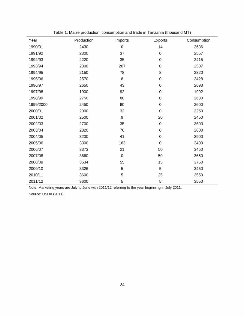
24

Table 1: Maize production, consumption and trade in Tanzania (thousand MT)

Year Production Imports Exports Consumption 1990/91 2430 0 14 2636 1991/92 2300 37 0 2557 1992/93 2220 35 0 2415 1993/94 2300 207 0 2507 1994/95 2150 78 8 2320 1995/96 2570 8 0 2428 1996/97 2650 43 0 2693 1997/98 1900 92 0 1992 1998/99 2750 80 0 2630 1999/2000 2450 80 0 2600 2000/01 2000 32 0 2250 2001/02 2500 9 20 2450 2002/03 2700 35 0 2600 2003/04 2320 76 0 2600 2004/05 3230 41 0 2900 2005/06 3300 163 0 3400 2006/07 3373 21 50 3450 2007/08 3660 0 50 3650 2008/09 3634 55 15 3750 2009/10 3326 5 5 3450 2010/11 3600 5 25 3550 2011/12 3600 5 5 3550 Note: Marketing years are July to June with 2011/12 referring to the year beginning in July 2011.

Source: USDA (2011).

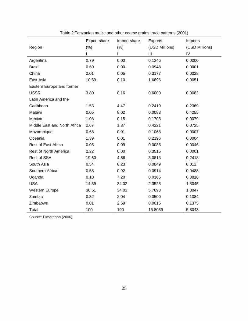
25

Table 2:Tanzanian maize and other coarse grains trade patterns (2001)

Region Export share (%)

Import share (%)

Exports (USD Millions)

Imports (USD Millions)

I II III IV Argentina 0.79 0.00 0.1246 0.0000 Brazil 0.60 0.00 0.0948 0.0001 China 2.01 0.05 0.3177 0.0028 East Asia 10.69 0.10 1.6896 0.0051 Eastern Europe and former USSR 3.80 0.16 0.6000 0.0082 Latin America and the Caribbean 1.53 4.47 0.2419 0.2369 Malawi 0.05 8.02 0.0083 0.4255 Mexico 1.08 0.15 0.1708 0.0079 Middle East and North Africa 2.67 1.37 0.4221 0.0725 Mozambique 0.68 0.01 0.1068 0.0007 Oceania 1.39 0.01 0.2196 0.0004 Rest of East Africa 0.05 0.09 0.0085 0.0046 Rest of North America 2.22 0.00 0.3515 0.0001 Rest of SSA 19.50 4.56 3.0813 0.2418 South Asia 0.54 0.23 0.0849 0.012 Southern Africa 0.58 0.92 0.0914 0.0488 Uganda 0.10 7.20 0.0165 0.3818 USA 14.89 34.02 2.3528 1.8045 Western Europe 36.51 34.02 5.7693 1.8047 Zambia 0.32 2.04 0.0500 0.1084 Zimbabwe 0.01 2.59 0.0015 0.1375 Total 100 100 15.8039 5.3043

Source: Dimaranan (2006).

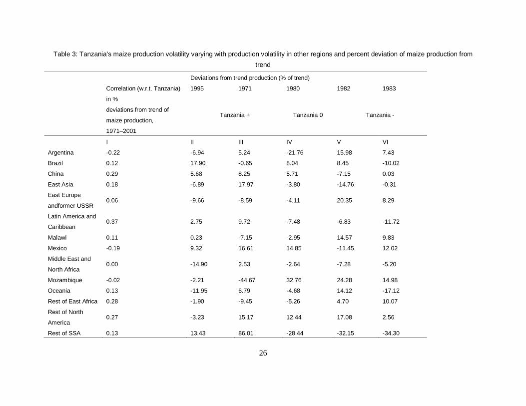
26

Table 3: Tanzania’s maize production volatility varying with production volatility in other regions and percent deviation of maize production from trend

Deviations from trend production (% of trend)

Correlation (w.r.t. Tanzania)

in %

deviations from trend of

maize production,

1971–2001

1995 1971 1980 1982 1983

Tanzania + Tanzania 0 Tanzania -

I II III IV V VI

Argentina -0.22 -6.94 5.24 -21.76 15.98 7.43

Brazil 0.12 17.90 -0.65 8.04 8.45 -10.02

China 0.29 5.68 8.25 5.71 -7.15 0.03

East Asia 0.18 -6.89 17.97 -3.80 -14.76 -0.31

East Europe

andformer USSR 0.06 -9.66 -8.59 -4.11 20.35 8.29

Latin America and

Caribbean 0.37 2.75 9.72 -7.48 -6.83 -11.72

Malawi 0.11 0.23 -7.15 -2.95 14.57 9.83

Mexico -0.19 9.32 16.61 14.85 -11.45 12.02

Middle East and

North Africa 0.00 -14.90 2.53 -2.64 -7.28 -5.20

Mozambique -0.02 -2.21 -44.67 32.76 24.28 14.98

Oceania 0.13 -11.95 6.79 -4.68 14.12 -17.12

Rest of East Africa 0.28 -1.90 -9.45 -5.26 4.70 10.07

Rest of North

America 0.27 -3.23 15.17 12.44 17.08 2.56

Rest of SSA 0.13 13.43 86.01 -28.44 -32.15 -34.30

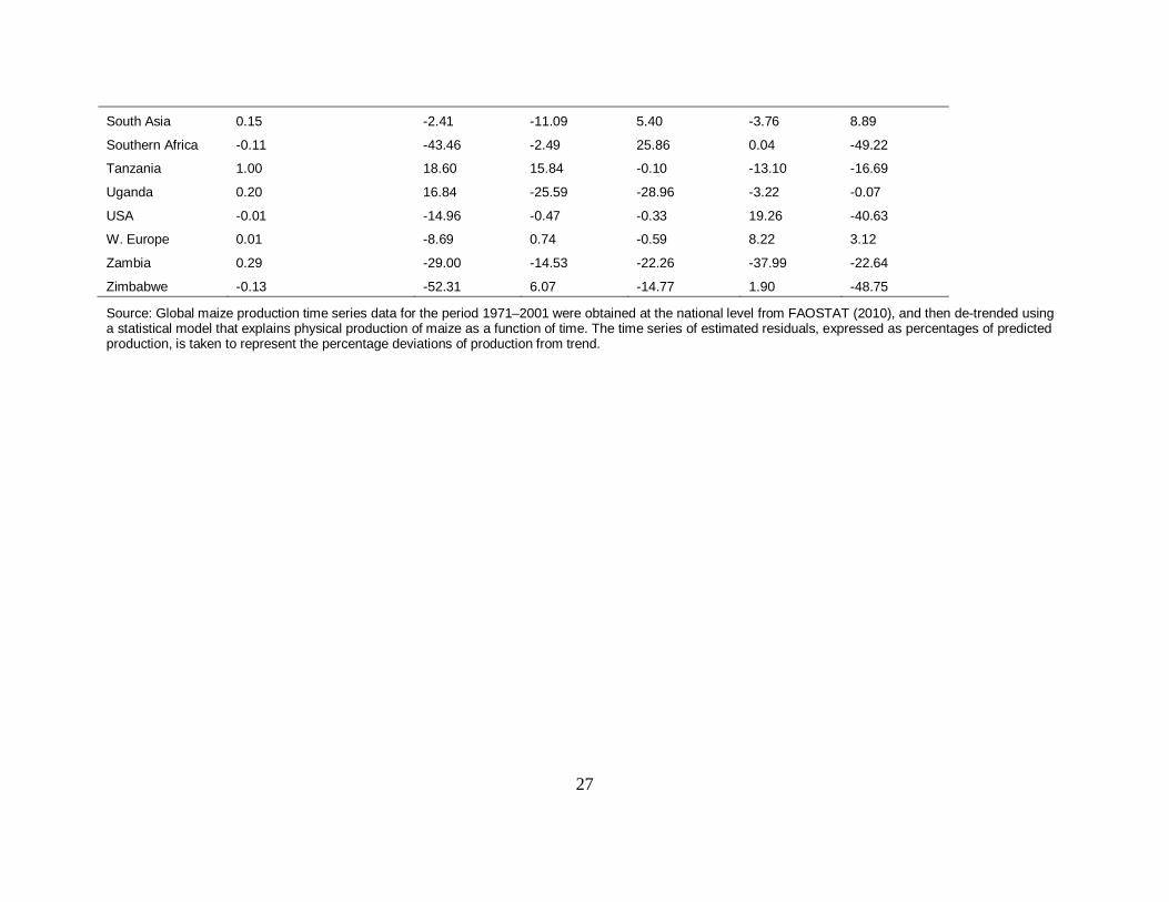
27

South Asia 0.15 -2.41 -11.09 5.40 -3.76 8.89

Southern Africa -0.11 -43.46 -2.49 25.86 0.04 -49.22

Tanzania 1.00 18.60 15.84 -0.10 -13.10 -16.69

Uganda 0.20 16.84 -25.59 -28.96 -3.22 -0.07

USA -0.01 -14.96 -0.47 -0.33 19.26 -40.63

W. Europe 0.01 -8.69 0.74 -0.59 8.22 3.12

Zambia 0.29 -29.00 -14.53 -22.26 -37.99 -22.64

Zimbabwe -0.13 -52.31 6.07 -14.77 1.90 -48.75

Source: Global maize production time series data for the period 1971–2001 were obtained at the national level from FAOSTAT (2010), and then de-trended using a statistical model that explains physical production of maize as a function of time. The time series of estimated residuals, expressed as percentages of predicted production, is taken to represent the percentage deviations of production from trend.

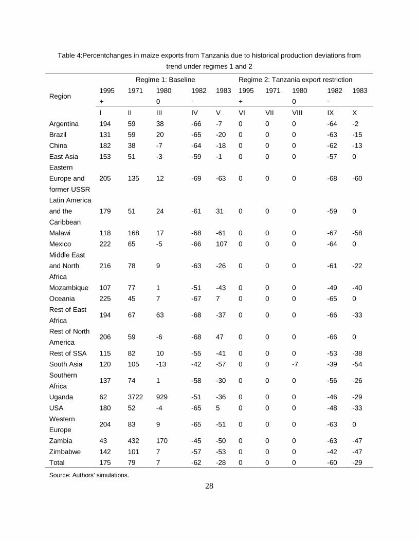
28

Table 4:Percentchanges in maize exports from Tanzania due to historical production deviations from trend under regimes 1 and 2

Region

Regime 1: Baseline Regime 2: Tanzania export restriction 1995 1971 1980 1982 1983 1995 1971 1980 1982 1983 + 0 - + 0 - I II III IV V VI VII VIII IX X

Argentina 194 59 38 -66 -7 0 0 0 -64 -2 Brazil 131 59 20 -65 -20 0 0 0 -63 -15 China 182 38 -7 -64 -18 0 0 0 -62 -13 East Asia 153 51 -3 -59 -1 0 0 0 -57 0 Eastern Europe and former USSR

205 135 12 -69 -63 0 0 0 -68 -60

Latin America and the Caribbean

179 51 24 -61 31 0 0 0 -59 0

Malawi 118 168 17 -68 -61 0 0 0 -67 -58 Mexico 222 65 -5 -66 107 0 0 0 -64 0 Middle East and North Africa

216 78 9 -63 -26 0 0 0 -61 -22

Mozambique 107 77 1 -51 -43 0 0 0 -49 -40 Oceania 225 45 7 -67 7 0 0 0 -65 0 Rest of East Africa

194 67 63 -68 -37 0 0 0 -66 -33

Rest of North America

206 59 -6 -68 47 0 0 0 -66 0

Rest of SSA 115 82 10 -55 -41 0 0 0 -53 -38 South Asia 120 105 -13 -42 -57 0 0 -7 -39 -54 Southern Africa

137 74 1 -58 -30 0 0 0 -56 -26

Uganda 62 3722 929 -51 -36 0 0 0 -46 -29 USA 180 52 -4 -65 5 0 0 0 -48 -33 Western Europe

204 83 9 -65 -51 0 0 0 -63 0

Zambia 43 432 170 -45 -50 0 0 0 -63 -47 Zimbabwe 142 101 7 -57 -53 0 0 0 -42 -47 Total 175 79 7 -62 -28 0 0 0 -60 -29

Source: Authors’ simulations.

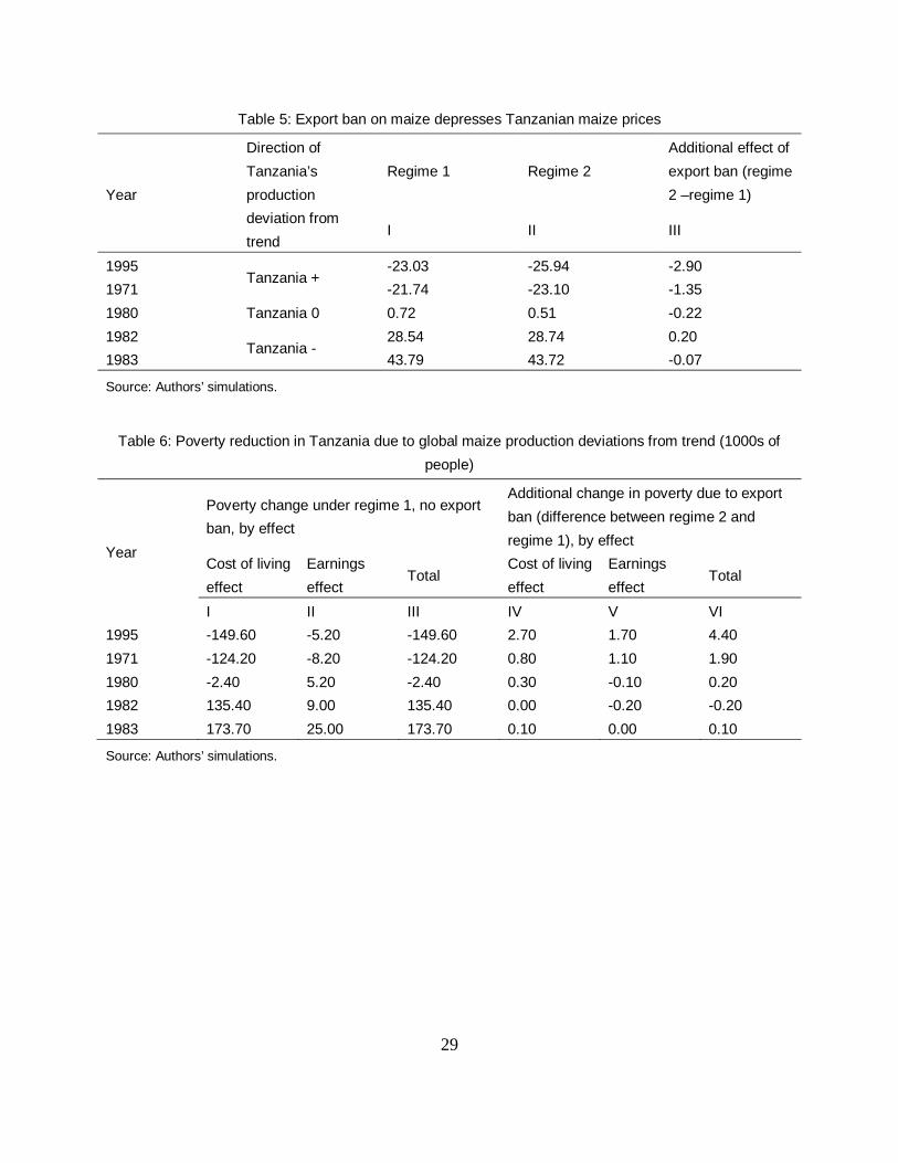
29

Table 5: Export ban on maize depresses Tanzanian maize prices

Year

Direction of Tanzania’s production deviation from trend

Regime 1 Regime 2 Additional effect of export ban (regime 2 –regime 1)

I II III

1995 Tanzania +

-23.03 -25.94 -2.90 1971 -21.74 -23.10 -1.35 1980 Tanzania 0 0.72 0.51 -0.22 1982

Tanzania - 28.54 28.74 0.20

1983 43.79 43.72 -0.07

Source: Authors’ simulations.

Table 6: Poverty reduction in Tanzania due to global maize production deviations from trend (1000s of people)

Year

Poverty change under regime 1, no export ban, by effect

Additional change in poverty due to export ban (difference between regime 2 and regime 1), by effect

Cost of living effect

Earnings effect

Total Cost of living effect

Earnings effect

Total

I II III IV V VI 1995 -149.60 -5.20 -149.60 2.70 1.70 4.40 1971 -124.20 -8.20 -124.20 0.80 1.10 1.90 1980 -2.40 5.20 -2.40 0.30 -0.10 0.20 1982 135.40 9.00 135.40 0.00 -0.20 -0.20 1983 173.70 25.00 173.70 0.10 0.00 0.10

Source: Authors’ simulations.

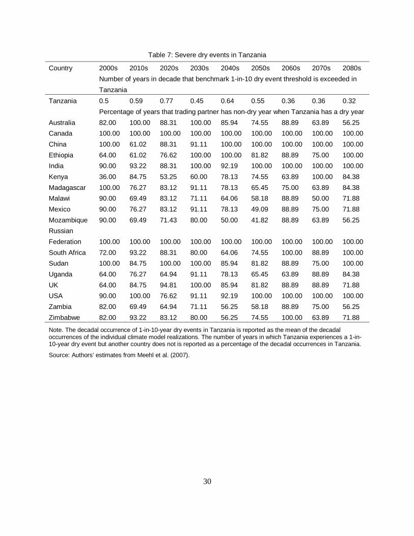
30

Table 7: Severe dry events in Tanzania

Country 2000s 2010s 2020s 2030s 2040s 2050s 2060s 2070s 2080s

Number of years in decade that benchmark 1-in-10 dry event threshold is exceeded in Tanzania

Tanzania 0.5 0.59 0.77 0.45 0.64 0.55 0.36 0.36 0.32 Percentage of years that trading partner has non-dry year when Tanzania has a dry year Australia 82.00 100.00 88.31 100.00 85.94 74.55 88.89 63.89 56.25 Canada 100.00 100.00 100.00 100.00 100.00 100.00 100.00 100.00 100.00 China 100.00 61.02 88.31 91.11 100.00 100.00 100.00 100.00 100.00 Ethiopia 64.00 61.02 76.62 100.00 100.00 81.82 88.89 75.00 100.00 India 90.00 93.22 88.31 100.00 92.19 100.00 100.00 100.00 100.00 Kenya 36.00 84.75 53.25 60.00 78.13 74.55 63.89 100.00 84.38 Madagascar 100.00 76.27 83.12 91.11 78.13 65.45 75.00 63.89 84.38 Malawi 90.00 69.49 83.12 71.11 64.06 58.18 88.89 50.00 71.88 Mexico 90.00 76.27 83.12 91.11 78.13 49.09 88.89 75.00 71.88 Mozambique 90.00 69.49 71.43 80.00 50.00 41.82 88.89 63.89 56.25 Russian Federation 100.00 100.00 100.00 100.00 100.00 100.00 100.00 100.00 100.00 South Africa 72.00 93.22 88.31 80.00 64.06 74.55 100.00 88.89 100.00 Sudan 100.00 84.75 100.00 100.00 85.94 81.82 88.89 75.00 100.00 Uganda 64.00 76.27 64.94 91.11 78.13 65.45 63.89 88.89 84.38 UK 64.00 84.75 94.81 100.00 85.94 81.82 88.89 88.89 71.88 USA 90.00 100.00 76.62 91.11 92.19 100.00 100.00 100.00 100.00 Zambia 82.00 69.49 64.94 71.11 56.25 58.18 88.89 75.00 56.25 Zimbabwe 82.00 93.22 83.12 80.00 56.25 74.55 100.00 63.89 71.88

Note. The decadal occurrence of 1-in-10-year dry events in Tanzania is reported as the mean of the decadal occurrences of the individual climate model realizations. The number of years in which Tanzania experiences a 1-in-10-year dry event but another country does not is reported as a percentage of the decadal occurrences in Tanzania.

Source: Authors’ estimates from Meehl et al. (2007).

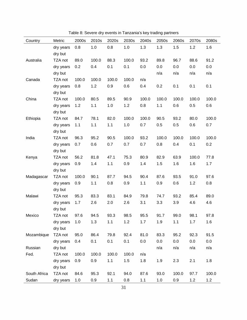
31

Table 8: Severe dry events in Tanzania’s key trading partners

Country Metric 2000s 2010s 2020s 2030s 2040s 2050s 2060s 2070s 2080s

Australia

dry years 0.8 1.0 0.8 1.0 1.3 1.3 1.5 1.2 1.6 dry but TZA not 89.0 100.0 88.3 100.0 93.2 89.8 96.7 88.6 91.2

Canada

dry years 0.2 0.4 0.1 0.1 0.0 0.0 0.0 0.0 0.0 dry but TZA not 100.0 100.0 100.0 100.0 n/a

n/a n/a n/a n/a

China

dry years 0.8 1.2 0.9 0.6 0.4 0.2 0.1 0.1 0.1 dry but TZA not 100.0 80.5 89.5 90.9 100.0 100.0 100.0 100.0 100.0

Ethiopia

dry years 1.2 1.1 1.0 1.2 0.8 1.1 0.6 0.5 0.6 dry but TZA not 84.7 78.1 82.0 100.0 100.0 90.5 93.2 80.0 100.0

India

dry years 1.1 1.1 1.1 1.0 0.7 0.5 0.5 0.6 0.7 dry but TZA not 96.3 95.2 90.5 100.0 93.2 100.0 100.0 100.0 100.0

Kenya

dry years 0.7 0.6 0.7 0.7 0.7 0.8 0.4 0.1 0.2 dry but TZA not 56.2 81.8 47.1 75.3 80.9 82.9 63.9 100.0 77.8

Madagascar

dry years 0.9 1.4 1.1 0.9 1.4 1.5 1.6 1.6 1.7 dry but TZA not 100.0 90.1 87.7 94.5 90.4 87.6 93.5 91.0 97.6

Malawi

dry years 0.9 1.1 0.8 0.9 1.1 0.9 0.6 1.2 0.8 dry but TZA not 95.3 83.3 83.1 84.9 79.8 74.7 93.2 85.4 89.0

Mexico

dry years 1.7 2.6 2.0 2.6 3.1 3.3 3.9 4.6 4.6 dry but TZA not 97.6 94.5 93.3 98.5 95.5 91.7 99.0 98.1 97.8

Mozambique

dry years 1.0 1.3 1.1 1.2 1.7 1.9 1.1 1.7 1.6 dry but TZA not 95.0 86.4 79.8 92.4 81.0 83.3 95.2 92.3 91.5

Russian Fed.

dry years 0.4 0.1 0.1 0.1 0.0 0.0 0.0 0.0 0.0 dry but TZA not 100.0 100.0 100.0 100.0 n/a

n/a n/a n/a n/a

South Africa

dry years 0.9 0.9 1.1 1.5 1.8 1.9 2.3 2.1 1.8 dry but TZA not 84.6 95.3 92.1 94.0 87.6 93.0 100.0 97.7 100.0

Sudan dry years 1.0 0.9 1.1 0.8 1.1 1.0 0.9 1.2 1.2

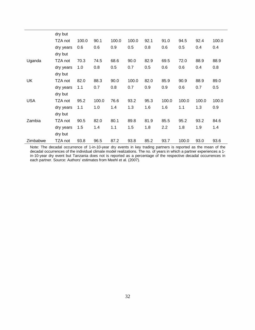
32

dry but TZA not 100.0 90.1 100.0 100.0 92.1 91.0 94.5 92.4 100.0

Uganda

dry years 0.6 0.6 0.9 0.5 0.8 0.6 0.5 0.4 0.4 dry but TZA not 70.3 74.5 68.6 90.0 82.9 69.5 72.0 88.9 88.9

UK

dry years 1.0 0.8 0.5 0.7 0.5 0.6 0.6 0.4 0.8 dry but TZA not 82.0 88.3 90.0 100.0 82.0 85.9 90.9 88.9 89.0

USA

dry years 1.1 0.7 0.8 0.7 0.9 0.9 0.6 0.7 0.5 dry but TZA not 95.2 100.0 76.6 93.2 95.3 100.0 100.0 100.0 100.0

Zambia

dry years 1.1 1.0 1.4 1.3 1.6 1.6 1.1 1.3 0.9 dry but TZA not 90.5 82.0 80.1 89.8 81.9 85.5 95.2 93.2 84.6

Zimbabwe

dry years 1.5 1.4 1.1 1.5 1.8 2.2 1.8 1.9 1.4 dry but TZA not 93.8 96.5 87.2 93.8 85.2 93.7 100.0 93.0 93.6

Note: The decadal occurrence of 1-in-10-year dry events in key trading partners is reported as the mean of the decadal occurrences of the individual climate model realizations. The no. of years in which a partner experiences a 1-in-10-year dry event but Tanzania does not is reported as a percentage of the respective decadal occurrences in each partner. Source: Authors’ estimates from Meehl et al. (2007).