A Practical Reachability-Based Collision Avoidance Algorithm forSampled-Data Systems: Application to Ground Robots

Charles Dabadie, Shahab Kaynama, and Claire J. Tomlin

Abstract— We describe a practical collision avoidance algo-rithm that synthesizes provably safe piecewise constant controllaws (compatible with the sampled-data nature of the system)for an experimental platform. Our application is formulated ina pursuer-evader framework in which an automated unmannedvehicle navigates its environment while avoiding a movingobstacle that acts as a malicious agent. Offline, we employreachability analysis to characterize the evolution of trajectoriesso as to determine what control inputs can preserve safetyover every sampling interval. The moving obstacle is consideredunpredictable with nearly no restrictions on its control policies(although we do take into account the physical constraints dueto limited dynamical and actuation capacities of both robots).Online, the controller executes computationally inexpensiveoperations based only on an easy-to-store lookup table. Theresults of the experiment as well as the proposed algorithm arepresented and discussed in detail.

I. INTRODUCTION

Collision avoidance is a central problem when dealingwith safety of autonomous vehicles such as unmanned air-craft and ground robots. Commonly, a safety distance isdefined around the vehicle and the goal is to keep otherobjects away from this perimeter.

Much research has been done in this domain, mainlythrough the concept of velocity obstacles (basically the setof velocities that would lead to collision with a movingobstacle). In [1], safe straight-line trajectories are built for ahost robot that faces multiple obstacles with constant velocityvectors, while in [2] velocity obstacles have been generalizedto the case of obstacles that move along arbitrary trajectories.Safety guarantees are obtained for either finite or infinite timehorizons. In [3], the concept of velocity obstacle has beenextended considering unicycle models for obstacles. The safepaths for the host robot are successions of lines that do notconsider the dynamical capacities or physical constraints ofthe robot during changes of heading or speed.

In [4], the problems of collision avoidance in the presenceof moving obstacles and path planning are solved simultane-ously in the joint state-time space via probabilistic roadmaps.A similar approach is that of rapidly-exploring random trees[5]. Other related techniques include the body of work on

This work has been supported in part by NSF under CPS:ActionWebs(CNS-931843), by ONR under the HUNT (N0014-08-0696) and SMARTS(N00014-09-1-1051) MURIs and by grant N00014-12-1-0609, by AFOSRunder the CHASE MURI (FA9550-10-1-0567).

S. Kaynama and C. Tomlin are with the Department of ElectricalEngineering and Computer Sciences, University of California at Berkeley,CA, USA. {kaynama, tomlin}@eecs.berkeley.edu

C. Dabadie is with Institut Superieur de l’Aeronautique et de l’Espace(Formation Supaero), Toulouse, France. c.dabadie@isae.fr

optimal trajectory generation and path planning in dynamicenvironments, e.g. through trajectory parameterization [6].

A numerical tool for solving the collision avoidance prob-lem is reachability analysis [7], [8]. Indeed, in many appli-cations, the systems under study are modeled by constrainednonlinear differential equations, and therefore analytical so-lutions for trajectories do not always exist. Reachabilityanalysis allows for controller design via numerical safetyverification of trajectories. The backward reachable set ofa given set A is the set of initial states that can be driveninto A by the constrained dynamical system. In the contextof collision avoidance, the reachable set formulation can beused to construct control policies that ensure safety of thevehicle despite the actions of a malicious agent. A classicalmethod for numerically computing the reachable set is viathe resolution of a terminal value Hamilton-Jacobi-Isaacs(HJI) partial differential equation [7], where one computesthe backward evolution of a level set function representingA using, for example, the method described in [9]. Thesafety-preserving control inputs are those that optimize theassociated Hamiltonian.

In this paper we primarily focus on an application of thereachability-based controller design to an experimental plat-form with two agents. The problem we consider is to designand implement a practical collision avoidance algorithm thatis to be mounted on board an automated unmanned groundvehicle (henceforth simply referred to as the UV) which isbeing chased by a human-operated robot (henceforth referredto as the moving obstacle, or simply the obstacle). Ourtestbed consists of two Pioneer robots [10] whose positionsare measured by a VICON system. This measurement isin turn fed into the UV and is used online to compute anappropriate course of action. The challenges we face includeproposing a provably-safe algorithm that is (a) light enoughto store and execute on an embedded microcontroller, (b)compatible with the sampled-data nature of the system (asampled-data system is one whose evolution is in continuoustime, yet it is driven by a digital, and hence discrete-time,controller that has access to state measurements/estimates ata fixed sampling frequency), and (c) flexible enough to allowthe UV to follow an objective when safety is not at stake.

Great progress has been made in reachability analysis ofconstrained, nonlinear sampled-data systems. The commonelement is to ensure conservatism when the control law isrestricted to the class of piecewise constant (PWC) functions(as opposed to the more common, and less stringent, class ofLebesgue measurable functions). For instance, in [11], [12] areach-avoid problem is considered where the goal is to reach

a given target set in finite time, and thereafter remain in aninvariant subset of the target while also avoiding a givenunsafe set. Similarly in [13], a projection-based techniqueis described that allows one to compute the sampled-datadiscriminating kernel (loosely speaking, the complement ofthe reachable set) and its associated control laws.

Here, we build upon these works and propose and apply acollision avoidance algorithm on our experimental platformsubject to the challenges described above. Our approach,similar to [11]–[13], is based on quantization of the controlset (the set from which the UV draws its input values)which maintains conservatism/safety while reducing the on-line computational burden. Most computations are handledoffline. The online computations, which are performed on theembedded microcontroller, are limited to forming an estimateof the state and executing basic arithmetic based on an easy-to-store lookup table (precomputed offline). Several conceptsare introduced to allow simple, practical implementation ofthe collision avoidance algorithm. For instance, we introducethe notion of freedom set which allows us to identify theregions of the state space in which all possible controlvalues can safely be applied to the system. The freedomset serves as an indicator when choosing optimal boundariesfor the numerical grid (over which the reachable set hasbeen computed) so as to minimize the data that is neededto be stored on the UV’s memory. To that end, we alsodescribe a method to account for the case in which astate estimate falls in between grid points. Doing so willwaive the need for employing a dense grid (which could beimpossible to store on limited memory), while still ensuringa reasonable degree of conservatism when choosing safety-preserving control values. We also discuss a technique thatallows for computation of certain regions of the state spacein which any nominal and arbitrary controller with access tothe original non-quantized control set could be used withoutthe fear of jeopardizing safety.

In Section III, we present a recursive algorithm for thecomputation of the sampled-data reachable set. We thendescribe how this set can be used to design a safety-preserving PWC control law. Section IV quantifies the errorintroduced when the state estimation does not yield valuesthat can be mapped exactly on the stored grid points. InSection V, we lay out the online algorithm which is real-ized using the open-source Robot Operating System (ROS)[14], while in Section VI the main experimental results arepresented in detail. Section VII discusses (and validates viasimulations) additional physically-motivated restrictions thatcan be placed on the input set of the obstacle so as to reducethe conservatism (as measured by the energy expenditure ofthe UV’s input signal) of our algorithm. Finally, concludingremarks and future works are provided in Section VIII.

II. PROBLEM FORMULATION

Consider a two-player differential game where the dynam-ics are governed by x = f(x, u, d) with x ∈ X , whereX ⊆ Rn is the state space. Here, u(·) is the control input ofthe UV, and d(·) is the control input of the moving obstacle.

For simplicity, we shall use the simplified notations u and dto denote both functions as well as their point-wise values;differentiating between these two types should be possiblevia the context in which they are used.

With a sampling time Ts > 0, we define the set of controlinputs for the UV over [−Ts, 0] as

C1 := {u : [−Ts, 0]→ U s.t. u constant on [−Ts, 0]} , (1)

where the input constraint set U is a compact subset of Rmu .To simplify our algorithm for the purpose of implementationon board the UV, we quantize the set U (which we denoteby Uq) and only consider a finite number of possible inputvalues. Therefore, the new set of control signals for the UVis

Cq1 := {u : [−Ts, 0]→ Uq s.t. u constant on [−Ts, 0]} .

(2)Note, however that the quantization of the input set maintainsour desired conservatism in the sense that all generatedcontrol laws by the algorithm are, as we shall see shortly,safety-preserving.

On the other hand, we define the set of control inputs forthe obstacle over [−Ts, 0] as

C2 := {d : [−Ts, 0]→ D s.t. d measurable on [−Ts, 0]} ,(3)

where the input constraint set D is a compact subset of Rmd .We do not restrict the control inputs of the obstacle as we didfor the UV because we want to allow any possible obstaclebehavior.

For a given set A, define its backward reachable set forfixed u ∈ Cq

1 over one sampling interval as

BA(A, u) := {x0 ∈ X : ∃d ∈ C2,∃t ∈ [−Ts, 0], xu,dx0

(t) ∈ A} (4)

with xu,dx0(t) the solution of x = f(x, u, d), x(−Ts) = x0.

To model the dynamics of the two agents (our automatedUV and the moving obstacle) on a 2D plane, we use theclassical pursuer-evader formulation. The UV acts as theevader and the obstacle as the pursuer. The relative dynamicscan be represented [7] by the continuous-time system

x =d

dt

x1

x2

x3

=

−u1 + d1 cos(x3) + u2x2

d1 sin(x3)− u2x1

d2 − u2

= f(x , u , d).

(5)The evader’s inputs are speed u1 and yaw rate u2. The

pursuer’s inputs d1 and d2 are similarly defined. x1 and x2

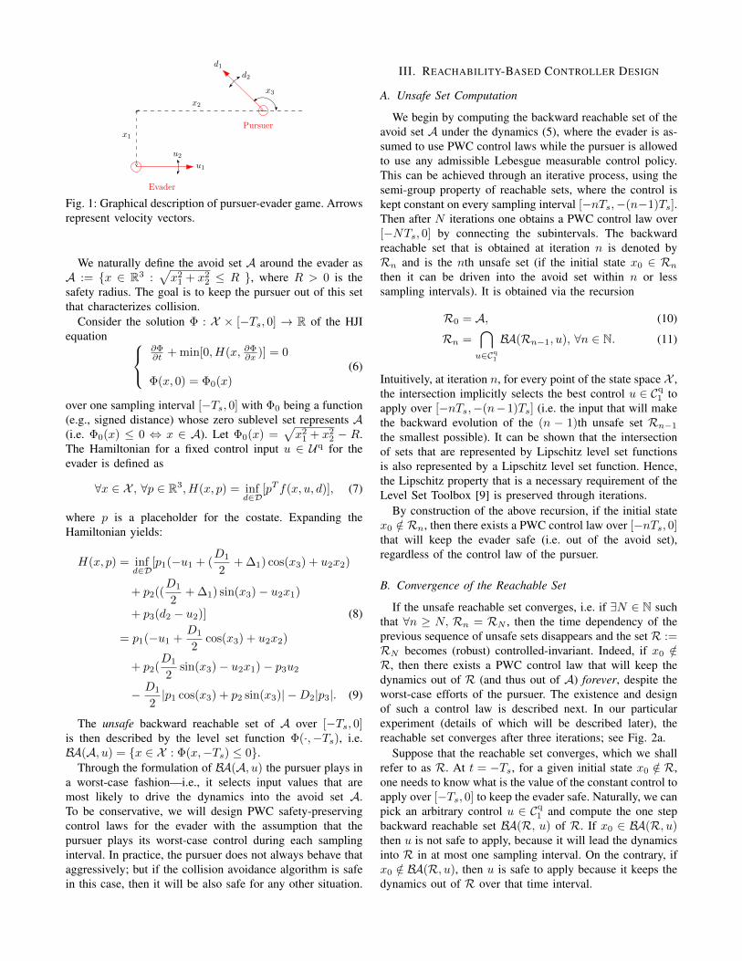
are Cartesian coordinates of the pursuer in the evader’s frame(centered at the evader, x-axis aligned with evader’s heading)and x3 is the relative angle between the evader’s and thepursuer’s headings; see Fig. 1 for a graphical description.The evader’s control input is defined and constrained asu := (u1, u2) ∈ Uq ⊂ U = [0, U1] × [−U2, U2] ⊆ R2.The pursuer’s control input is defined and constrained asd := (∆1, d2) ∈ D = [−D1

2 ,D1

2 ] × [−D2, D2] ⊆ R2 where∆1 = d1 − D1

2 (we shifted d1 to simplify the Hamiltonian(9)).

x1

x2

x3

u1

u2

d1d2

Evader

Pursuer

Fig. 1: Graphical description of pursuer-evader game. Arrowsrepresent velocity vectors.

We naturally define the avoid set A around the evader asA := {x ∈ R3 :

√x2

1 + x22 ≤ R }, where R > 0 is the

safety radius. The goal is to keep the pursuer out of this setthat characterizes collision.

Consider the solution Φ : X × [−Ts, 0] → R of the HJIequation

∂Φ∂t + min[0, H(x, ∂Φ

∂x )] = 0

Φ(x, 0) = Φ0(x)(6)

over one sampling interval [−Ts, 0] with Φ0 being a function(e.g., signed distance) whose zero sublevel set represents A(i.e. Φ0(x) ≤ 0 ⇔ x ∈ A). Let Φ0(x) =

√x2

1 + x22 − R.

The Hamiltonian for a fixed control input u ∈ Uq for theevader is defined as

∀x ∈ X , ∀p ∈ R3, H(x, p) = infd∈D

[pT f(x, u, d)], (7)

where p is a placeholder for the costate. Expanding theHamiltonian yields:

H(x, p) = infd∈D

[p1(−u1 + (D1

2+ ∆1) cos(x3) + u2x2)

+ p2((D1

2+ ∆1) sin(x3)− u2x1)

+ p3(d2 − u2)] (8)

= p1(−u1 +D1

2cos(x3) + u2x2)

+ p2(D1

2sin(x3)− u2x1)− p3u2

− D1

2|p1 cos(x3) + p2 sin(x3)| −D2|p3|. (9)

The unsafe backward reachable set of A over [−Ts, 0]is then described by the level set function Φ(·,−Ts), i.e.BA(A, u) = {x ∈ X : Φ(x,−Ts) ≤ 0}.

Through the formulation of BA(A, u) the pursuer plays ina worst-case fashion—i.e., it selects input values that aremost likely to drive the dynamics into the avoid set A.To be conservative, we will design PWC safety-preservingcontrol laws for the evader with the assumption that thepursuer plays its worst-case control during each samplinginterval. In practice, the pursuer does not always behave thataggressively; but if the collision avoidance algorithm is safein this case, then it will be also safe for any other situation.

III. REACHABILITY-BASED CONTROLLER DESIGN

A. Unsafe Set Computation

We begin by computing the backward reachable set of theavoid set A under the dynamics (5), where the evader is as-sumed to use PWC control laws while the pursuer is allowedto use any admissible Lebesgue measurable control policy.This can be achieved through an iterative process, using thesemi-group property of reachable sets, where the control iskept constant on every sampling interval [−nTs,−(n−1)Ts].Then after N iterations one obtains a PWC control law over[−NTs, 0] by connecting the subintervals. The backwardreachable set that is obtained at iteration n is denoted byRn and is the nth unsafe set (if the initial state x0 ∈ Rn

then it can be driven into the avoid set within n or lesssampling intervals). It is obtained via the recursion

R0 = A, (10)

Rn =⋂

u∈Cq1

BA(Rn−1, u), ∀n ∈ N. (11)

Intuitively, at iteration n, for every point of the state space X ,the intersection implicitly selects the best control u ∈ Cq

1 toapply over [−nTs,−(n−1)Ts] (i.e. the input that will makethe backward evolution of the (n − 1)th unsafe set Rn−1

the smallest possible). It can be shown that the intersectionof sets that are represented by Lipschitz level set functionsis also represented by a Lipschitz level set function. Hence,the Lipschitz property that is a necessary requirement of theLevel Set Toolbox [9] is preserved through iterations.

By construction of the above recursion, if the initial statex0 /∈ Rn, then there exists a PWC control law over [−nTs, 0]that will keep the evader safe (i.e. out of the avoid set),regardless of the control law of the pursuer.

B. Convergence of the Reachable Set

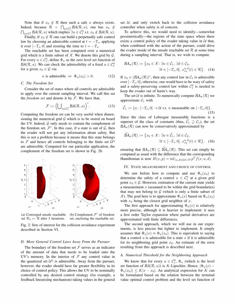
If the unsafe reachable set converges, i.e. if ∃N ∈ N suchthat ∀n ≥ N, Rn = RN , then the time dependency of theprevious sequence of unsafe sets disappears and the set R :=RN becomes (robust) controlled-invariant. Indeed, if x0 /∈R, then there exists a PWC control law that will keep thedynamics out of R (and thus out of A) forever, despite theworst-case efforts of the pursuer. The existence and designof such a control law is described next. In our particularexperiment (details of which will be described later), thereachable set converges after three iterations; see Fig. 2a.

Suppose that the reachable set converges, which we shallrefer to as R. At t = −Ts, for a given initial state x0 /∈ R,one needs to know what is the value of the constant control toapply over [−Ts, 0] to keep the evader safe. Naturally, we canpick an arbitrary control u ∈ Cq

1 and compute the one stepbackward reachable set BA(R, u) of R. If x0 ∈ BA(R, u)then u is not safe to apply, because it will lead the dynamicsinto R in at most one sampling interval. On the contrary, ifx0 /∈ BA(R, u), then u is safe to apply because it keeps thedynamics out of R over that time interval.

Note that if x0 /∈ R then such a safe u always exists.Indeed, because R =

⋂u∈Cq1

BA(R, u), one has x0 /∈⋂u∈Cq1

BA(R, u) which implies ∃u ∈ Cq1 s.t. x0 /∈ BA(R, u).

Finally, if x0 /∈ R one can build a perpetually safe controllaw by choosing an admissible control at t = −Ts, applyingit over [−Ts, 0] and reseting the time to t = −Ts.

The reachable set has been computed over a numericalgrid which is a finite subset of X . We denote this grid by G.For every u ∈ Cq

1 , define Φu as the zero level set function ofBA(R, u). We can check the admissibility of a fixed u ∈ Cq

1

for a given x0 ∈ G via

u is admissible ⇔ Φu(x0) > 0. (12)

C. The Freedom Set

Consider the set of states where all controls are admissibleto apply over the current sampling interval. We call this setthe freedom set and denote it by F . We have that,

F :=(⋃

u∈Cq1BA(R, u)

)c. (13)

Computing the freedom set can be very useful when dimen-sioning the numerical grid G which is to be stored on boardthe UV. Indeed, G only needs to contain the complement ofthe freedom set, Fc. In this case, if a state is out of G, thenthe evader will not get any information about safety. Butthis is not a problem because it means that this state belongsto F and hence all controls belonging to the finite set Uq

are admissible. Computed for our particular application, thecomplement of the freedom set is shown in Fig. 2b.

(a) Converged unsafe reachableset R3 =: R after 3 iterations.

(b) Complement Fc of freedomset, enclosing the reachable set.

Fig. 2: Sets of interest for the collision avoidance experimentdescribed in Section VI.

D. More General Control Laws Away From the Pursuer

The boundary of the freedom set F serves as an indicatorof the amount of data that needs to be loaded onto theUV’s memory. In the interior of F any control value inthe quantized set Uq is admissible. Away from the pursuer,however, the evader should have far greater flexibility in itschoice of control policy. This allows the UV to be nominallycontrolled by any desired control strategy (for example, afeedback linearizing mechanism) taking values in the general

set U , and only switch back to the collision avoidancecontroller when safety is of concern.

To achieve this, we would need to identify—somewhatpessimistically—the regions of the state space where thereexists a control policy of the evader taking value in U that,when combined with the action of the pursuer, could drivethe evader inside of the unsafe reachable set R at some timeduring a sampling interval. That is, we wish to compute

BAw(R) :={x0 ∈ X : ∃u ∈ C1, ∃d ∈ C2,

∃t ∈ [−Ts, 0], xu,dx0(t) ∈ R

}. (14)

If x0 ∈ (BAw(R))c, then any control law in C1 is admissibleover [−Ts, 0]; otherwise, one would have to be wary of safetyand a safety-preserving control law within Cq

1 is needed tokeep the evader out of harm’s way.

The set U is infinite. To numerically compute BAw(R) weapproximate C1 with

C1 := {u : [−Ts, 0]→ U s.t. u measurable on [−Ts, 0]} .(15)

Since the class of Lebesgue measurable functions is asuperset of the class of constants (thus, C1 ⊇ C1), the setBAw(R) can now be conservatively approximated by

BAw(R) :={x0 ∈ X : ∃u ∈ C1, ∃d ∈ C2,

∃t ∈ [−Ts, 0], xu,dx0(t) ∈ R

}, (16)

ensuring that BAw(R) ⊆ BAw(R). This set can simply becomputed as usual with the difference that the correspondingHamiltonian is now H(x, p) = inf(u,d)∈U×D p

T f(x, u, d).

IV. STATE MEASUREMENT AND CHOICE OF CONTROL

We saw before how to compute and use Φu(x0) todetermine the safety of a control u ∈ Cq

1 at a given gridpoint x0 ∈ G. However, estimation of the current state yieldsa measurement x (assumed to be within the grid boundaries)that may not belong to G (which is only a finite subset ofX ). The goal here is to approximate Φu(x) based on Φu(x0)with x0 being the closest grid neighbor of x.

The first approach for approximating Φu(x) is relativelymore precise, although it is heavier to implement: it usesa first order Taylor expansion where partial derivatives areapproximated with finite differences.

The second approach, which we will use in our exper-iments, is less precise but lighter to implement. It simplyassumes that Φu(x) ≈ Φu(x0). This is equivalent to sayingthat a control u is admissible for a state x if it is admissiblefor its neighboring grid point x0. An estimate of the errorresulting from this approach is described next.

A. Numerical Threshold for the Neighboring Approach

We know that for every u ∈ Cq1 , Φu (which is the level

set function of BA(R, u)) is K-Lipschitz. Hence, |Φu(x)−Φu(x0)| ≤ K|x − x0|. An analytical expression for K canbe formulated based on the relation between the terminalvalue optimal control problem and the level set function of

the reachable set [15]. For brevity, however, we refrain fromdiscussing these results in the current paper.

Let us assume the grid has constant spacings in everydirection. Let ∆xi be the spacing along the xi direction ∀i ∈{1, 2, 3}. Then, since x0 is the closest grid point to x, wehave |x−x0| ≤ 1

2

√(∆x1)2 + (∆x2)2 + (∆x3)2. Denote the

numerical error as ε := K 12

√(∆x1)2 + (∆x2)2 + (∆x3)2

so that for any x that is within the bounds of the grid, for itscorresponding closest grid neighbor x0, and ∀u ∈ Cq

1 one has|Φu(x) − Φu(x0)| ≤ ε. In (12) we saw a decision criterionbased on the sign of Φu(x0). We can adapt this criterion totake into account the fact that the estimated state x may fallin between grid points:

u is admissible at x ⇔ Φu(x0) > ε, (17)

where x0 is the closest neighboring grid point to x.This new decision threshold is going to reduce the size

of the freedom set F . Intuitively, some controls that used tobe admissible before are no longer admissible since our newdecision criterion is more conservative. This implies that theevader starts having a safety reaction earlier than before. Thenew freedom set is F = {x ∈ X : minu∈Cq1 Φu(x) > ε}.

V. ONLINE ALGORITHM

We implemented our collision avoidance algorithm onground robots via the Robot Operating System (ROS) [14] inC++. Based on the presented offline computations, we formour online algorithm as follows. The main data are the valuesof Φu(x0), ∀(u, x0) ∈ Cq

1 ×G which we store into an arrayand load onto the UV’s memory.

1) At t = −Ts, update measurements, which are positionsand headings of the pursuer and the evader. A headingis obtained by measuring two successive positions at100 Hz. Reconstruct 3D state vector x.

2) If the estimated vector falls within the grid’s bounds,find the closest grid neighbor x0; Otherwise, all con-trols are admissible and proceed to step 4.

3) For every u ∈ Cq1 , check the sign of Φu(x0) − ε.

This gives us the set of admissible, safety-preservingcontrols.

4) Among these controls, choose one that fulfills a giventask (such as reaching an objective).

5) Apply the chosen control law during the current timeinterval (t = −Ts to t = 0). Reset the time variablet← −Ts, and restart from step 1.

We robustify our online algorithm against measurementnoise, delay, and numerical errors by increasing the valueof the threshold ε. For our experiment we empirically foundthis value to be ε = 0.5 m.

Finally, it may happen that due to experimental approxi-mations the obstacle would come too close to the boundaryof the reachable set (though it still remains outside of it).Then at step 3 of the above algorithm, there would notbe any u ∈ Cq

1 verifying Φu(x0) − ε > 0. In this casethe evader should play its best effort control defined asubest(x0) ∈ arg maxu∈Cq1 {Φu(x0)}.

VI. EXPERIMENTS

A. Setup

We used two Pioneer ground robots [10]. The first onewas automated with the collision avoidance algorithm andplayed the role of the evader. The second one was re-motely controlled by a human operator and played the roleof the pursuer. We used VICON system to get positionmeasurements. We set the maximum speeds of the robotsto U1 = D1 = 0.15 m/s and the maximum yaw rates toU2 = D2 = 1 rad/s (these values were obtained basedon the robots’ physical capacities). Finally, we assumedthat Pioneer ground robots follow unicycle models, i.e. theycan be controlled in terms of velocity vector’s magnitudeand angular rate. This assumption is fairly accurate whenconsidering this type of robot which has a physical heading(the direction from the rear to the front). That being said, therobot is not using a steering mechanism (as one would expectin a vehicle that follows a unicycle model), but instead it isapplying differential rotating speeds to the wheels in order toturn (which introduces additional drifting). The kinematicsare described by the following simple nonlinear model:

x = v cos(ψ)y = v sin(ψ)

ψ = ω.(18)

Therefore, we assume that we can directly control the speedv and the yaw rate ω.

The evader’s objective is to reach the plane’s origin. Atevery iteration of the algorithm, it synthesizes the set of safeyaw rate values, and picks one that would orient its velocityvector the closest toward the direction of the objective.Finally, to simplify the implementations, we fixed the speedof the evader to its maximum value. Therefore, the onlyactual control input is the yaw rate. The set of consideredcontrol values Uq that appears in the definition of Cq

1 in (1)is

Uq = {0.15} × {−1 ,−0.5 , 0 , 0.5 , 1}, (19)

where the speed has been fixed to 0.15 m/s and the yaw ratevalues are given in rad/s. As discussed earlier, such quanti-zation maintains conservatism and formalism. Qualitatively,the inputs drawn from Uq allow the evader to go straight andto turn left or right more or less quickly.

Finally, we fixed the sampling time as Ts = 1 s. Thesampling frequency of the collision avoidance algorithm canbe chosen as desired (though it must be the same in bothoffline and online calculations) as long as it is slower thanthat of the internal lower-level control unit inside of therobots, as well as the sampling frequency of the measurementsensors used in the state estimator. Also, we fixed the safetyradius as R = 0.8 m. This value has been chosen basedon the size of the robots, so that as long as the pursuer’scenter is further than 0.8 m away from the evader’s centerthen collision has not occurred.

With the previously described numerical values, the reach-able set converges after 3 iterations (Fig. 2a). The grid’s sizewas of 60 points in each direction. The offline computational

−3 −2 −1 0 1 2 3−0.8

−0.6

−0.4

−0.2

0

0.2

0.4

0.6

0.8

1

x (m)

y (m

)

evaderpursuer

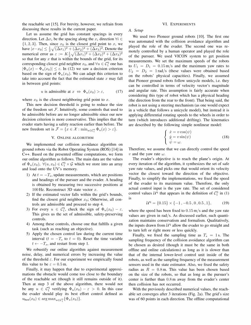
Fig. 3: Absolute trajectories in x-y plane. The objective isrepresented by a blue cross. Small black circles/diamondsrepresent the start/end of trajectories.

time of the converged unsafe reachable set was approxi-mately 15 mins.1 We used 8 MB of on board memory to storethe values of the level set function Φu on the UV. We applythe collision avoidance algorithm described in Section V.

B. Results

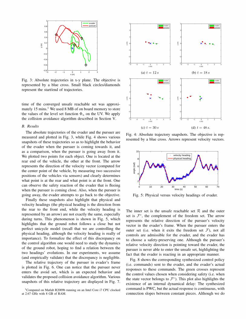
The absolute trajectories of the evader and the pursuer aremeasured and plotted in Fig. 3, while Fig. 4 shows varioussnapshots of these trajectories so as to highlight the behaviorof the evader when the pursuer is coming towards it, andas a comparison, when the pursuer is going away from it.We plotted two points for each object. One is located at therear end of the vehicle, the other at the front. The arrowrepresents the direction of the velocity vector (computed forthe center point of the vehicle, by measuring two successivepositions of the vehicles via sensors) and clearly determineswhat point is at the rear and what point is at the front. Onecan observe the safety reaction of the evader that is fleeingwhen the pursuer is coming close. Also, when the pursuer isgoing away, the evader attempts to go back to the objective.

Finally these snapshots also highlight that physical andvelocity headings (the physical heading is the direction fromthe rear to the front end, while the velocity heading isrepresented by an arrow) are not exactly the same, especiallyduring turns. This phenomenon is shown in Fig. 5, whichhighlights that the ground robot follows a close but notperfect unicycle model (recall that we are controlling thephysical heading, although the velocity heading is really ofimportance). To formalize the effect of this discrepancy onthe control algorithm one would need to study the dynamicsof the ground robot, hoping to find a relation between thetwo headings’ evolutions. In our experiments, we assume(and empirically validate) that the discrepancy is negligible.

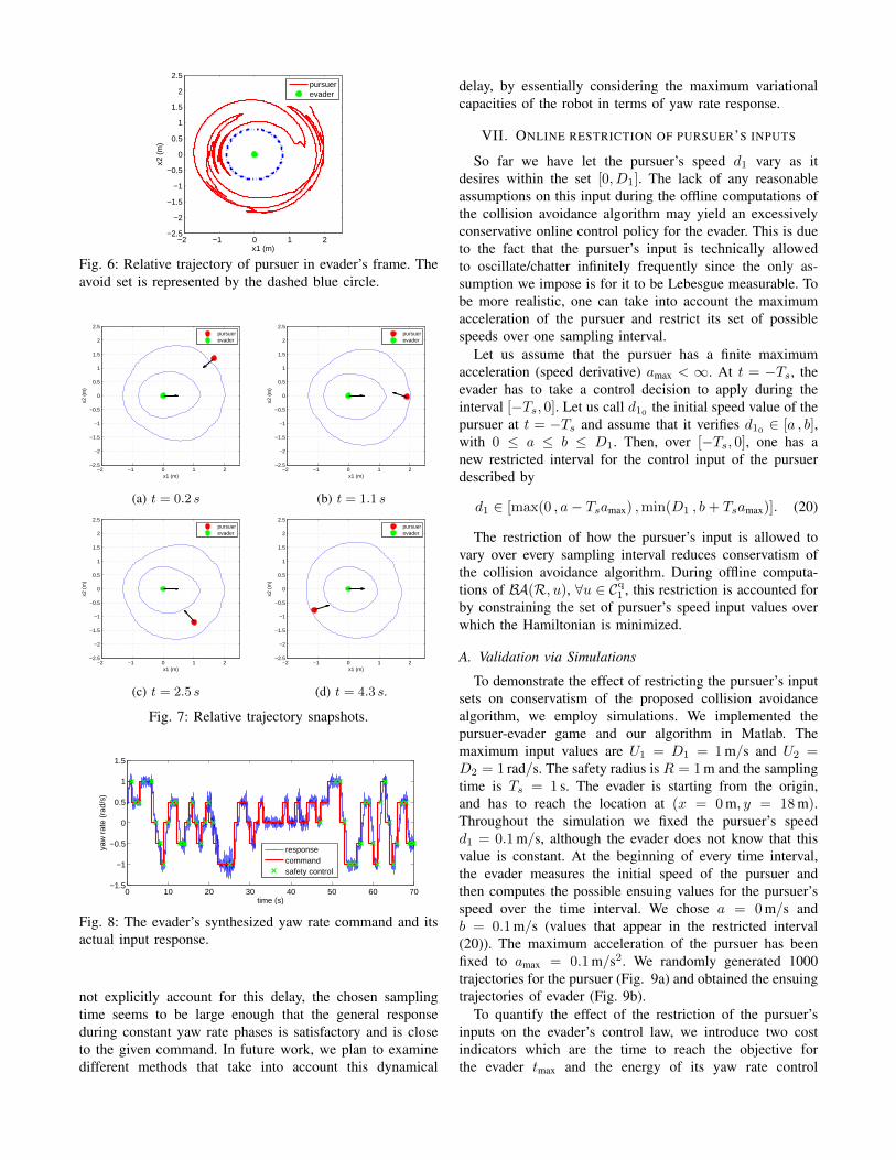
The relative trajectory of the pursuer in evader’s frameis plotted in Fig. 6. One can notice that the pursuer neverenters the avoid set, which is an expected behavior andvalidates the proposed collision avoidance algorithm. Varioussnapshots of this relative trajectory are displayed in Fig. 7.

1Computed on Matlab R2009b running on an Intel Core i7 CPU clockedat 2.67 GHz with 8 GB of RAM.

−3 −2 −1 0 1 2 3−3

−2

−1

0

1

2

3

x (m)

y (m

)

evaderpursuer

(a) t = 12 s

−3 −2 −1 0 1 2 3−3

−2

−1

0

1

2

3

x (m)

y (m

)

evaderpursuer

(b) t = 18 s

−3 −2 −1 0 1 2 3−3

−2

−1

0

1

2

3

x (m)

y (m

)

evaderpursuer

(c) t = 30 s

−3 −2 −1 0 1 2 3−3

−2

−1

0

1

2

3

x (m)

y (m

)

evaderpursuer

(d) t = 48 s.

Fig. 4: Absolute trajectory snapshots. The objective is rep-resented by a blue cross. Arrows represent velocity vectors.

0 10 20 30 40 50 60 70

2

4

6

8

10

time (s)

angl

e (r

ad)

velocity headingphysical heading

Fig. 5: Physical versus velocity headings of evader.

The inner set is the unsafe reachable set R and the outerset is Fc, the complement of the freedom set. The arrowrepresents the relative direction of the pursuer’s velocityvector in the evader’s frame. When the pursuer enters theouter set (i.e. when it exits the freedom set F), not allcontrols are admissible for the evader, and the evader hasto choose a safety-preserving one. Although the pursuer’srelative velocity direction is pointing toward the evader, thepursuer is never able to enter the unsafe set, highlighting thefact that the evader is reacting in an appropriate manner.

Fig. 8 shows the corresponding synthesized control policy(i.e. commands) sent to the evader, and the evader’s actualresponses to these commands. The green crosses representthe control values chosen when considering safety (i.e. whenthe state vector belongs to Fc). This plot also highlights theexistence of an internal dynamical delay: The synthesizedcommand is PWC, but the actual response is continuous, withconnection slopes between constant pieces. Although we do

−2 −1 0 1 2−2.5

−2

−1.5

−1

−0.5

0

0.5

1

1.5

2

2.5

x1 (m)

x2 (

m)

pursuerevader

Fig. 6: Relative trajectory of pursuer in evader’s frame. Theavoid set is represented by the dashed blue circle.

−2 −1 0 1 2−2.5

−2

−1.5

−1

−0.5

0

0.5

1

1.5

2

2.5

x1 (m)

x2 (

m)

pursuerevader

(a) t = 0.2 s

−2 −1 0 1 2−2.5

−2

−1.5

−1

−0.5

0

0.5

1

1.5

2

2.5

x1 (m)

x2 (

m)

pursuerevader

(b) t = 1.1 s

−2 −1 0 1 2−2.5

−2

−1.5

−1

−0.5

0

0.5

1

1.5

2

2.5

x1 (m)

x2 (

m)

pursuerevader

(c) t = 2.5 s

−2 −1 0 1 2−2.5

−2

−1.5

−1

−0.5

0

0.5

1

1.5

2

2.5

x1 (m)

x2 (

m)

pursuerevader

(d) t = 4.3 s.

Fig. 7: Relative trajectory snapshots.

0 10 20 30 40 50 60 70−1.5

−1

−0.5

0

0.5

1

1.5

time (s)

yaw

rat

e (r

ad/s

)

responsecommandsafety control

Fig. 8: The evader’s synthesized yaw rate command and itsactual input response.

not explicitly account for this delay, the chosen samplingtime seems to be large enough that the general responseduring constant yaw rate phases is satisfactory and is closeto the given command. In future work, we plan to examinedifferent methods that take into account this dynamical

delay, by essentially considering the maximum variationalcapacities of the robot in terms of yaw rate response.

VII. ONLINE RESTRICTION OF PURSUER’S INPUTS

So far we have let the pursuer’s speed d1 vary as itdesires within the set [0, D1]. The lack of any reasonableassumptions on this input during the offline computations ofthe collision avoidance algorithm may yield an excessivelyconservative online control policy for the evader. This is dueto the fact that the pursuer’s input is technically allowedto oscillate/chatter infinitely frequently since the only as-sumption we impose is for it to be Lebesgue measurable. Tobe more realistic, one can take into account the maximumacceleration of the pursuer and restrict its set of possiblespeeds over one sampling interval.

Let us assume that the pursuer has a finite maximumacceleration (speed derivative) amax < ∞. At t = −Ts, theevader has to take a control decision to apply during theinterval [−Ts, 0]. Let us call d10

the initial speed value of thepursuer at t = −Ts and assume that it verifies d10 ∈ [a , b],with 0 ≤ a ≤ b ≤ D1. Then, over [−Ts, 0], one has anew restricted interval for the control input of the pursuerdescribed by

d1 ∈ [max(0 , a− Tsamax) ,min(D1 , b+ Tsamax)]. (20)

The restriction of how the pursuer’s input is allowed tovary over every sampling interval reduces conservatism ofthe collision avoidance algorithm. During offline computa-tions of BA(R, u), ∀u ∈ Cq

1 , this restriction is accounted forby constraining the set of pursuer’s speed input values overwhich the Hamiltonian is minimized.

A. Validation via Simulations

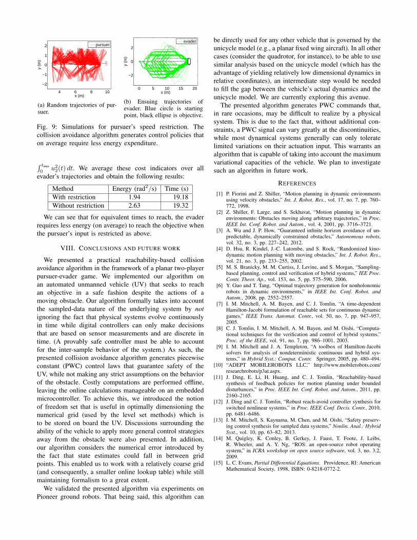
To demonstrate the effect of restricting the pursuer’s inputsets on conservatism of the proposed collision avoidancealgorithm, we employ simulations. We implemented thepursuer-evader game and our algorithm in Matlab. Themaximum input values are U1 = D1 = 1 m/s and U2 =D2 = 1 rad/s. The safety radius is R = 1 m and the samplingtime is Ts = 1 s. The evader is starting from the origin,and has to reach the location at (x = 0 m, y = 18 m).Throughout the simulation we fixed the pursuer’s speedd1 = 0.1 m/s, although the evader does not know that thisvalue is constant. At the beginning of every time interval,the evader measures the initial speed of the pursuer andthen computes the possible ensuing values for the pursuer’sspeed over the time interval. We chose a = 0 m/s andb = 0.1 m/s (values that appear in the restricted interval(20)). The maximum acceleration of the pursuer has beenfixed to amax = 0.1 m/s2. We randomly generated 1000trajectories for the pursuer (Fig. 9a) and obtained the ensuingtrajectories of evader (Fig. 9b).

To quantify the effect of the restriction of the pursuer’sinputs on the evader’s control law, we introduce two costindicators which are the time to reach the objective forthe evader tmax and the energy of its yaw rate control

4 6 8 10

−2

−1

0

1

2

x (m)

y (m

)

pursuer

(a) Random trajectories of pur-suer.

0 5 10 15 20

−2

0

2

x (m)

y (m

)

evader

(b) Ensuing trajectories ofevader. Blue circle is startingpoint, black ellipse is objective.

Fig. 9: Simulations for pursuer’s speed restriction. Thecollision avoidance algorithm generates control policies thaton average require less energy expenditure.

∫ tmax

0u2

2(t) dt. We average these cost indicators over allevader’s trajectories and obtain the following results:

Method Energy (rad2/s) Time (s)With restriction 1.94 19.18Without restriction 2.63 19.32

We can see that for equivalent times to reach, the evaderrequires less energy (on average) to reach the objective whenthe pursuer’s input is restricted as above.

VIII. CONCLUSIONS AND FUTURE WORK

We presented a practical reachability-based collisionavoidance algorithm in the framework of a planar two-playerpursuer-evader game. We implemented our algorithm onan automated unmanned vehicle (UV) that seeks to reachan objective in a safe fashion despite the actions of amoving obstacle. Our algorithm formally takes into accountthe sampled-data nature of the underlying system by notignoring the fact that physical systems evolve continuouslyin time while digital controllers can only make decisionsthat are based on sensor measurements and are discrete intime. (A provably safe controller must be able to accountfor the inter-sample behavior of the system.) As such, thepresented collision avoidance algorithm generates piecewiseconstant (PWC) control laws that guarantee safety of theUV, while not making any strict assumptions on the behaviorof the obstacle. Costly computations are performed offline,leaving the online calculations manageable on an embeddedmicrocontroller. To achieve this, we introduced the notionof freedom set that is useful in optimally dimensioning thenumerical grid (used by the level set methods) which isto be stored on board the UV. Discussions surrounding theability of the vehicle to apply more general control strategiesaway from the obstacle were also presented. In addition,our algorithm considers the numerical error introduced bythe fact that state estimates could fall in between gridpoints. This enabled us to work with a relatively coarse grid(and consequently, a smaller online lookup table) while stillmaintaining formalism to a great extent.

We validated the presented algorithm via experiments onPioneer ground robots. That being said, this algorithm can

be directly used for any other vehicle that is governed by theunicycle model (e.g., a planar fixed wing aircraft). In all othercases (consider the quadrotor, for instance), to be able to usesimilar analysis based on the unicycle model (which has theadvantage of yielding relatively low dimensional dynamics inrelative coordinates), an intermediate step would be neededto fill the gap between the vehicle’s actual dynamics and theunicycle model. We are currently exploring this avenue.

The presented algorithm generates PWC commands that,in rare occasions, may be difficult to realize by a physicalsystem. This is due to the fact that, without additional con-straints, a PWC signal can vary greatly at the discontinuities,while most dynamical systems generally can only toleratelimited variations on their actuation input. This warrants analgorithm that is capable of taking into account the maximumvariational capacities of the vehicle. We plan to investigatesuch an algorithm in future work.

REFERENCES

[1] P. Fiorini and Z. Shiller, “Motion planning in dynamic environmentsusing velocity obstacles,” Int. J. Robot. Res., vol. 17, no. 7, pp. 760–772, 1998.

[2] Z. Shiller, F. Large, and S. Sekhavat, “Motion planning in dynamicenvironments: Obstacles moving along arbitrary trajectories,” in Proc.IEEE Int. Conf. Robot. and Autom., vol. 4, 2001, pp. 3716–3721.

[3] A. Wu and J. P. How, “Guaranteed infinite horizon avoidance of un-predictable, dynamically constrained obstacles,” Autonomous robots,vol. 32, no. 3, pp. 227–242, 2012.

[4] D. Hsu, R. Kindel, J.-C. Latombe, and S. Rock, “Randomized kino-dynamic motion planning with moving obstacles,” Int. J. Robot. Res.,vol. 21, no. 3, pp. 233–255, 2002.

[5] M. S. Branicky, M. M. Curtiss, J. Levine, and S. Morgan, “Sampling-based planning, control and verification of hybrid systems,” IEE Proc.Contr. Theor. Ap., vol. 153, no. 5, pp. 575–590, 2006.

[6] Y. Guo and T. Tang, “Optimal trajectory generation for nonholonomicrobots in dynamic environments,” in IEEE Int. Conf. Robot. andAutom., 2008, pp. 2552–2557.

[7] I. M. Mitchell, A. M. Bayen, and C. J. Tomlin, “A time-dependentHamilton-Jacobi formulation of reachable sets for continuous dynamicgames,” IEEE Trans. Automat. Contr., vol. 50, no. 7, pp. 947–957,2005.

[8] C. J. Tomlin, I. M. Mitchell, A. M. Bayen, and M. Oishi, “Computa-tional techniques for the verification and control of hybrid systems,”Proc. of the IEEE, vol. 91, no. 7, pp. 986–1001, 2003.

[9] I. M. Mitchell and J. A. Templeton, “A toolbox of Hamilton-Jacobisolvers for analysis of nondeterministic continuous and hybrid sys-tems,” in Hybrid Syst.: Comput. Contr. Springer, 2005, pp. 480–494.

[10] “ADEPT MOBILEROBOTS LLC,” http://www.mobilerobots.com/researchrobots/p3at.aspx.

[11] J. Ding, E. Li, H. Huang, and C. J. Tomlin, “Reachability-basedsynthesis of feedback policies for motion planning under boundeddisturbances,” in Proc. IEEE Int. Conf. Robot. and Autom., 2011, pp.2160–2165.

[12] J. Ding and C. J. Tomlin, “Robust reach-avoid controller synthesis forswitched nonlinear systems,” in Proc. IEEE Conf. Decis. Contr., 2010,pp. 6481–6486.

[13] I. M. Mitchell, S. Kaynama, M. Chen, and M. Oishi, “Safety preserv-ing control synthesis for sampled data systems,” Nonlin. Anal.: HybridSyst., vol. 10, pp. 63–82, 2013.

[14] M. Quigley, K. Conley, B. Gerkey, J. Faust, T. Foote, J. Leibs,R. Wheeler, and A. Y. Ng, “ROS: an open-source robot operatingsystem,” in ICRA workshop on open source software, vol. 3, no. 3.2,2009.

[15] L. C. Evans, Partial Differential Equations. Providence, RI: AmericanMathematical Society, 1998, ISBN: 0-8218-0772-2.