Embed Size (px)
Citation preview
Collision Avoidance ManeuverOptimization
A Fast and Accurate Semi-analytical Approach
Trabajo Fin de Master (TFM)Master Universitario en Ingenierıa Aeroespacial
Escuela Tecnica Superior de Ingenieros Aeronauticos
Universidad Politecnica de Madrid
19 Septiembre 2014
Author: Javier Hernando Ayuso
Supervisor: Claudio Bombardelli

Contents
1 Introduction 1
1.1 Background . . . . . . . . . . . . . . . . . . . . . . . . . . . . . . . . . . 1
1.2 Conjunction Summary Message . . . . . . . . . . . . . . . . . . . . . . . 2
1.3 Collision avoidance maneuvers . . . . . . . . . . . . . . . . . . . . . . . . 3
2 Impulsive maneuver dynamics 5
2.1 Introduction . . . . . . . . . . . . . . . . . . . . . . . . . . . . . . . . . . 5
2.2 Reference systems. Transformations . . . . . . . . . . . . . . . . . . . . . 5
2.2.1 Perifocal Reference frame . . . . . . . . . . . . . . . . . . . . . . 5
2.2.2 Frenet Reference Frame (TNH) . . . . . . . . . . . . . . . . . . . 5
2.2.3 UVW reference frame . . . . . . . . . . . . . . . . . . . . . . . . . 6
2.2.4 The b-plane . . . . . . . . . . . . . . . . . . . . . . . . . . . . . . 7
2.3 Short encounter hypothesis . . . . . . . . . . . . . . . . . . . . . . . . . . 8
2.4 Analytical impulsive maneuver approximation . . . . . . . . . . . . . . . 8
2.5 Impulse orientation angles . . . . . . . . . . . . . . . . . . . . . . . . . . 11
3 Orbit uncertainty 13
3.1 Introduction . . . . . . . . . . . . . . . . . . . . . . . . . . . . . . . . . . 13
3.2 Some notes on probability theory . . . . . . . . . . . . . . . . . . . . . . 13
3.3 Covariance matrix . . . . . . . . . . . . . . . . . . . . . . . . . . . . . . 14
3.3.1 Relative position covariance matrices . . . . . . . . . . . . . . . . 15
3.4 Error ellipsoid . . . . . . . . . . . . . . . . . . . . . . . . . . . . . . . . . 15
3.5 Gaussian distribution . . . . . . . . . . . . . . . . . . . . . . . . . . . . . 16
4 Collision probability calculation 17
4.1 Introduction . . . . . . . . . . . . . . . . . . . . . . . . . . . . . . . . . . 17
4.2 The three-dimensional collision integral . . . . . . . . . . . . . . . . . . . 17
4.3 Chan’s method . . . . . . . . . . . . . . . . . . . . . . . . . . . . . . . . 18
4.3.1 The isotropic problem . . . . . . . . . . . . . . . . . . . . . . . . 18
4.3.2 The general case . . . . . . . . . . . . . . . . . . . . . . . . . . . 22
4.4 Other methods . . . . . . . . . . . . . . . . . . . . . . . . . . . . . . . . 25
4.4.1 Foster’s Method . . . . . . . . . . . . . . . . . . . . . . . . . . . . 25
4.4.2 Patera’s Method . . . . . . . . . . . . . . . . . . . . . . . . . . . 26
4.4.3 Alfano’s method . . . . . . . . . . . . . . . . . . . . . . . . . . . 26
4.4.4 Akella and Alfriend’s method . . . . . . . . . . . . . . . . . . . . 28
i
5 Collision avoidance maneuver optimization 295.1 Introduction . . . . . . . . . . . . . . . . . . . . . . . . . . . . . . . . . . 295.2 Some notes on optimization theory . . . . . . . . . . . . . . . . . . . . . 29
5.2.1 Unconstrained optimization . . . . . . . . . . . . . . . . . . . . . 295.2.2 Constrained optimization . . . . . . . . . . . . . . . . . . . . . . . 30
5.3 Direct Impact . . . . . . . . . . . . . . . . . . . . . . . . . . . . . . . . . 315.3.1 Maximum miss distance . . . . . . . . . . . . . . . . . . . . . . . 325.3.2 Minimum collision probability . . . . . . . . . . . . . . . . . . . . 335.3.3 Discussion . . . . . . . . . . . . . . . . . . . . . . . . . . . . . . . 34
5.4 Non-Direct Impact . . . . . . . . . . . . . . . . . . . . . . . . . . . . . . 355.4.1 Maximum miss distance . . . . . . . . . . . . . . . . . . . . . . . 355.4.2 An implicit constraint . . . . . . . . . . . . . . . . . . . . . . . . 375.4.3 Reachable Domain . . . . . . . . . . . . . . . . . . . . . . . . . . 385.4.4 Solution discontinuities . . . . . . . . . . . . . . . . . . . . . . . . 385.4.5 Minimum impulse magnitude for fixed collision probability . . . . 40
6 Numerical cases. Accuracy of the method 436.1 Introduction . . . . . . . . . . . . . . . . . . . . . . . . . . . . . . . . . . 436.2 Iridium-Cosmos Collision . . . . . . . . . . . . . . . . . . . . . . . . . . . 43
6.2.1 Direct-Impact (DI) . . . . . . . . . . . . . . . . . . . . . . . . . . 446.2.2 Non-Direct-Impact (NDI) . . . . . . . . . . . . . . . . . . . . . . 496.2.3 Solution Discontinuity . . . . . . . . . . . . . . . . . . . . . . . . 53
6.3 RapidEye4-UoSat2 Conjunction . . . . . . . . . . . . . . . . . . . . . . . 556.4 Accuracy of the method . . . . . . . . . . . . . . . . . . . . . . . . . . . 57
6.4.1 Iridium-Cosmos J2 error . . . . . . . . . . . . . . . . . . . . . . . 576.4.2 Near-head-on J2 error . . . . . . . . . . . . . . . . . . . . . . . . 586.4.3 Low altitude, near-head-on drag error . . . . . . . . . . . . . . . . 59
7 OCCAM 617.1 Introduction . . . . . . . . . . . . . . . . . . . . . . . . . . . . . . . . . . 617.2 How to use . . . . . . . . . . . . . . . . . . . . . . . . . . . . . . . . . . 617.3 OCCAM Collision avoidance Files (.odf) . . . . . . . . . . . . . . . . . . 637.4 OCCAM lite . . . . . . . . . . . . . . . . . . . . . . . . . . . . . . . . . . 63
8 Conclusions 698.1 Main contributions of this Thesis work . . . . . . . . . . . . . . . . . . . 698.2 Publications . . . . . . . . . . . . . . . . . . . . . . . . . . . . . . . . . . 708.3 Registered software . . . . . . . . . . . . . . . . . . . . . . . . . . . . . . 70
ii
List of Figures
2.1 Rotation from v1 to v2. . . . . . . . . . . . . . . . . . . . . . . . . . . . 7
4.1 The isotropic problem. . . . . . . . . . . . . . . . . . . . . . . . . . . . . 194.2 Rician probability density function. . . . . . . . . . . . . . . . . . . . . . 204.3 The general case. . . . . . . . . . . . . . . . . . . . . . . . . . . . . . . . 234.4 The general case. Axis scaling. . . . . . . . . . . . . . . . . . . . . . . . . 24
5.1 Ellipse and ellipse evolute with a = 2, b = 1. . . . . . . . . . . . . . . . . 395.2 Smooth (left, re = 3.5) and discontinuous (right, re = 1.1) solutions, with
a = 2, b = 1. . . . . . . . . . . . . . . . . . . . . . . . . . . . . . . . . . . 40
6.1 Iridium-Cosmos direct impact: Miss distance. . . . . . . . . . . . . . . . 456.2 Iridium-Cosmos direct impact: Collision probability. . . . . . . . . . . . . 456.3 Iridium-Cosmos direct impact: b-plane track (Prograde maneuver). . . . 466.4 Iridium-Cosmos direct impact: b-plane track (Retrograde maneuver). . . 466.5 Iridium-Cosmos direct impact: optimal in-plane orientation angle σ (Pro-
grade maneuver). . . . . . . . . . . . . . . . . . . . . . . . . . . . . . . . 476.6 Iridium-Cosmos direct impact: optimal in-plane orientation angle σ (Ret-
rograde maneuver). . . . . . . . . . . . . . . . . . . . . . . . . . . . . . . 476.7 Iridium-Cosmos direct impact: optimal out-of-plane orientation angle γ
(Prograde maneuver). . . . . . . . . . . . . . . . . . . . . . . . . . . . . . 486.8 Iridium-Cosmos direct impact: optimal out-of-plane orientation angle γ
(Retrograde maneuver). . . . . . . . . . . . . . . . . . . . . . . . . . . . 486.9 Iridium-Cosmos Non-Direct-Impact: Miss distance. . . . . . . . . . . . . 506.10 Iridium-Cosmos Non-Direct-Impact: Collision probability. . . . . . . . . . 506.11 Iridium-Cosmos Non-Direct-Impact: b-plane track. . . . . . . . . . . . . 516.12 Detail of Iridium-Cosmos Non-Direct-Impact: b-plane track. . . . . . . . 516.13 Iridium-Cosmos Non-Direct-Impact: optimal in-plane orientation angle σ. 526.14 Iridium-Cosmos Non-Direct-Impact: optimal out-of-plane orientation an-
gle γ. . . . . . . . . . . . . . . . . . . . . . . . . . . . . . . . . . . . . . . 526.15 Iridium-Cosmos Non-Direct-Impact: b-plane track after ∆θ. . . . . . . . 546.16 RapidEye4-UoSat2 minimum ∆V for a required collision probability. . . 566.17 RapidEye4-UoSat2 optimal in-plane maneuver angle σ for a required col-
lision probability. . . . . . . . . . . . . . . . . . . . . . . . . . . . . . . . 566.18 RapidEye4-UoSat2 optimal out-of-plane maneuver angle γ for a required
collision probability. . . . . . . . . . . . . . . . . . . . . . . . . . . . . . . 566.19 Iridium-Cosmos Keplerian and J2 error (left) and maximum miss distance
(right). . . . . . . . . . . . . . . . . . . . . . . . . . . . . . . . . . . . . . 576.20 Near-Head-on Keplerian and J2 error (left) and maximum miss distance
(right). . . . . . . . . . . . . . . . . . . . . . . . . . . . . . . . . . . . . . 58
iii
6.21 Low altitude, near-head-on Keplerian and atmospheric error (left) andmaximum miss distance (right). . . . . . . . . . . . . . . . . . . . . . . . 59
7.1 OCCAM user interface . . . . . . . . . . . . . . . . . . . . . . . . . . . . 627.2 OCCAM lite user interface . . . . . . . . . . . . . . . . . . . . . . . . . . 657.3 Iridium-Cosmos direct impact: Miss distance optimal orientation angles
using OCCAM lite . . . . . . . . . . . . . . . . . . . . . . . . . . . . . . 667.4 Iridium-Cosmos direct impact: Miss distance optimal orientation angles
using OCCAM . . . . . . . . . . . . . . . . . . . . . . . . . . . . . . . . 67
iv
Chapter 1
Introduction
1.1 Background
As a collateral damage of the use of space by military, scientific and commercial spacecraftmissions, tens of thousands of derelict objects have been left in orbit around our planet.They are usually referred as space debris, and their number is growing year by year [1, 2].The population of space debris is diverse in size, orbit an origin.
While fragmentation or break-ups of satellites or rocket bodies (intentional or not)produces debris with a wide range of sizes, the smallest fragments are also constituted byaluminum oxide (Al2O3) particles exhausted by solid rocket motors, the Russian ROR-SATs (Radar Ocean Reconnaissance Satellites) coolant liquid solidified droplets, andpaint or heat shield flaking or peeling. Additionally, out-of-life satellites and upper stagerocket bodies represent a large population of big-size, non-controllable bodies in EarthOrbit.
The distribution of debris is not uniform in space. Detailed distribution are presentedin [1, pp. 14, 15], and here the main points are highlighted.
Most of the objects are in a nearly circular orbit. Very low altitude orbits are depletedby the action of the atmospheric drag, and low earth orbit objects have a limited lifespan.However most of the satellites are located at low orbits, which implies a relatively highdensity of objects including, rocket bodies and derelict satellites. Some satellites performa burn at the end of their lives and change their orbit to a less interesting region of space,but the most important peaks after Low Earth Orbit are at around 26000 km (Mol-niya orbits and Geosynchronous Transfer orbits) and the Geosynchronous orbit (GEO)region. The later has a crucial economical importance, and the region is crowded withactive satellites and mission-related debris, and consequently non-functional satellites areusually removed from GEO after their mission has ended.
Regarding the inclination distribution, there are two clear concentration zones: in-clinations around 98 degrees correspond to sun-synchronous orbits, while the objects atapproximately 82 degrees have a similar global coverage but beneficiate from a slightlyincreased mass budget due to the lower inclination of the orbit compared to the sun-synchronous bodies. Another important peaks appear at around 0 degrees (GEO) and60 degrees.
A conjunction or close approach occurs when two bodies become closer in space thana certain threshold at some given epoch. The conjuncting objects may be two activesatellites, an active satellite and a piece of space debris, or both pieces of space debris. InNovember 2010, the U.S. military claimed they detected an average of 190 conjunctions
1
2 CHAPTER 1. INTRODUCTION
per week [2]. These conjunctions may lead to a collision between the bodies, causingminor damages, major damages or even mission termination or body fragmentation.
It is precisely the body fragmentation problem what lead Kessler to define the Colli-sional Cascading concept, commonly known as the Kessler Syndrome [3, 4]. The KesslerSyndrome describes an scenario such as that the rate of creation of new pieces of spacedebris grows exponentially caused by collisions between existing objects, rendering theuse of space around the Earth unfeasible.
Not all the satellite fragmentations are caused by collisions: some break-up eventsare associated to explosions (produced by the propulsion system or by a electrical systemfailure for example). Additionally, a considerable amount of objects of the space debrispopulation has been produced by Anti-satellite weapons (ASAT). One example of thelatter is the destruction of the Chinese weather satellite Fengyun-1C by the same countryin January 11 2007, which generated more than 2000 trackable pieces and a estimatednumber of several tens of thousands smaller objects.
In order to mitigate the problem of space debris, several strategies have been developed[1, pp. 165-198]. Some passive options seek reducing the number of objects generatedin a mission or preventing on-orbit explosions (emptying the remaining fluid inside thetanks once the mission has finished, for example). Among the active strategies, thereare three that should be mentioned: post-mission disposal, removal of passive items andcollision avoidance maneuvers between trackable objects. The post-mission disposal relieson the spacecraft removing itself from orbit once its mission has ended, reentering theatmosphere if possible, or transferring to a graveyard orbit if not. Removal of passiveitems is still a developing technology that seeks to perform post-mission disposal toa second inactive satellite or rocket body, evacuating it from a useful orbit. Finally,collision avoidance maneuvers are small orbital corrections performed in order to reducethe collision probability between two conjuncting objects.
1.2 Conjunction Summary Message
The Conjunction Summary Message (CSM) is a document issued by the United States AirForce’s Joint Space Operations Center (JSpOC) [5] that contains information related to aclose approach between a satellite and a secondary body. It is sent to the operator of thespacecraft and is not available to the public, but uses a format with open specifications.
The document contains information about the primary satellite (called asset), thesecondary body (called conjuncting satellite), and the conjuncting epoch. Additionally, itincludes position and uncertainty at the predicted closest approach. Note that the CSMdoes not contain any direct indication about whether a collision avoidance maneuveris necessary, and does not suggest any collision avoidance maneuver, neither in time,orientation or fuel consumption. The data provided allows a satellite operator to evaluatethe risk the conjunction poses, and to design a suitable collision avoidance maneuver thatalso takes into account the requirements of the mission.
The full format of the Conjunction Summary Message as well as an example CSMare publicly available in Reference [5]. The reference frame used is described in detail insection 2.2.3 of this work.
1.3. COLLISION AVOIDANCE MANEUVERS 3
1.3 Collision avoidance maneuvers
If a conjunction between an active satellite and another body is detected, it is possible toperform a collision avoidance maneuver if it poses a significative risk to the mission. Theusual criteria consists on exceeding a collision probability threshold or a safety distancein some direction [6]. Typically a safety box with different sizes in different directionsis used, for example for the ISS a box of ±0.75 km, ±25 km, ±25 km in the radial,along-track and out-of-planet directions is used [1, pp. 213-240]).
With the increase of the population of bodies in Earth Orbit (active satellites or spacedebris), the rate of collision avoidance maneuvers has been increasing in the last years. Asa part of the November 2010 report already mentioned above, the U.S military informedthat the satellite operators performed an average of three collision avoidance maneuversper week at that time. While collision avoidance maneuvers are small orbital correctionswith a low fuel consumption, they are performed with increasing frequency and can takean important fraction of the fuel budget of the satellite. Consequently, it is very importantto design efficient and accurate methods and algorithms to calculate optimal maneuvers,or at least maneuvers with high performance. This will lead to decreasing the ∆V budgetneeded for this purpose, allowing extension of the mission.
The typical collision avoidance maneuver consists on a small impulse generated by ashort burn by a rocket engine to prevent the collision, and a posterior orbital correctionif needed to restore the original orbit. The velocity changes involved are smaller than theorbital velocity, and usually are in the range of tens of mm/s. Determining the requiredmagnitude, the orientation of the impulse and the timing is the challenging problem thiswork tries to give an answer to.
The calculation of collision avoidance maneuvers is usually integrated into specificmaneuver planning software programmes [7, 8]. These tools usually perform parametricsearches and evaluate each case with a full numerical integration, resulting in a highcomputational cost. Another aspect that delay the calculations is the determinationof the collision probability, which plays an essential role in determining whether themaneuver is necessary, and the required magnitude in the affirmative case. Some authorsuse more sophisticated optimization methods [9, 10] which speed up the process, butstill require to propagate the orbit numerically and to deal with the collision probabilitycalculation.
In this work, fast analytical and semi-analytical methods will be proposed to solve theproblem of calculating an optimal collision avoidance maneuver at some epoch before theconjunction. A linearization of the equations of relative motion following an impulsivemaneuver [11] allows evaluating in an efficient way the effect of a ∆V , and using analyticalmethod to calculate the collision probability [12] the maneuver optimization problem isreduce to solving an eigenvalue problem in the case of zero miss-distance (direct-impact)[13], or an eigenvalue problem and a non-linear equation in the case of a non-direct-impact[14].
The structure of this work is as follows: Chapter 2 defines the reference frames to beused and describes the relative motion after an impulsive maneuver. Chapter 3 introducesthe concept of the uncertainty in the determination of the orbit. Chapter 4 analyzes thecollision probability calculation, describing in great detail the Chan’s Method, and someother methods as a comparison. Chapter 5 describes a novel algorithm for calculatingoptimal collision avoidance maneuvers in a fast, accurate and efficient way. Chapter 6contains numerical examples of some real mission scenarios where a collision avoidance

4 CHAPTER 1. INTRODUCTION
was necessary, as well a analysis of the accuracy of the present formulation. Chapter 7introduces a new software tool that implements the present formulation. Finally, chapter8 summarizes the advances presented in the present work.
Chapter 2
Impulsive maneuver dynamics
2.1 Introduction
After performing a Collision Avoidance maneuver, it is important to understand themotion of the maneuverable object with respect to the secondary body. The most generalapproach is to integrate the equations of motion after applying the impulse, but in order todevelop a fast method to calculate the optimal Collision Avoidance maneuver, it is usefulto use an approximation of the maneuverable object motion. However it is importantto ensure that such approximation is accurate enough, otherwise the result will not bereliable.
In this chapter, first we will define the necessary reference systems, as well as thetransformations between them and the corresponding geometric relations. Then, themain hypothesis that allows a fast and accurate computation will be proposed: the short-term encounter hypothesis. Finally, the linearization of the equation of relative motionafter an impulse maneuver will be exposed, which provides an analytical solution for theproblem.
This chapter is supported by the references [11], [12] and [15].
2.2 Reference systems. Transformations
2.2.1 Perifocal Reference frame
Let us suppose two objects in orbit around the Earth, S1 and S2. We will consider S1
as the maneuverable satellite, and define < X, Y, Z > as its perifocal reference frame.This is, X is defined along the (unperturbed) eccentricity vector and Z orthogonal to theorbital plane. The perifocal frame may be defined for both the body 1 and for the body2, but but only the perifocal frame of the body 1 will be used.
2.2.2 Frenet Reference Frame (TNH)
The second reference system to be employed is the Frenet reference frame (TNH). Thisreference frame has its first axis pointing in the tangent (T) direction, the second in thenormal (N) direction pointing inwards, and the third in the binormal direction (H, sinceit coincides with the angular momentum in this case). This reference frame is usuallyreferred to as TNH. TNH reference frame for the body 1 and for the body 2 will be used.
5
6 CHAPTER 2. IMPULSIVE MANEUVER DYNAMICS
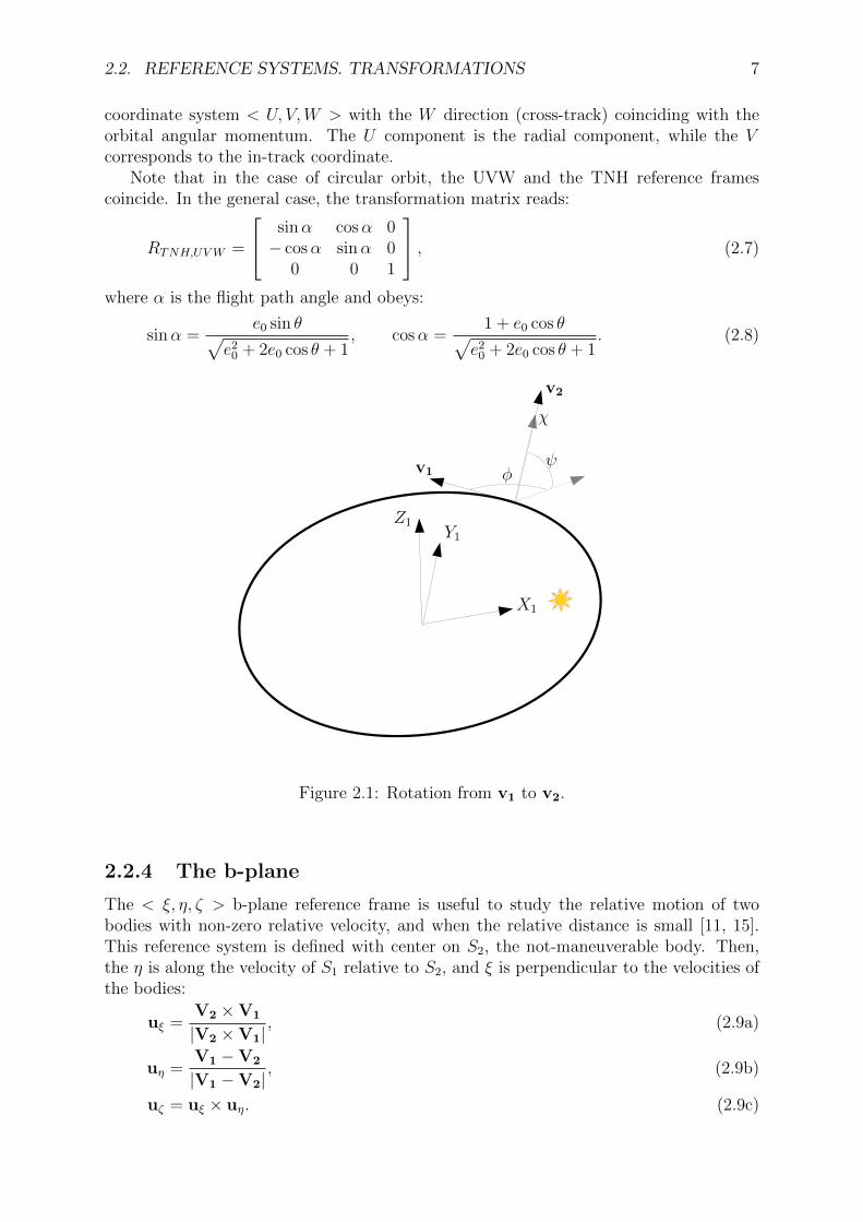
For some value of the true anomaly θ = θc, let us suppose that the two objects positioncoincides (later this will be referred as collision, or conjunction if some miss distance isallowed). At this point, the velocity of the second body can be obtained via two rotationsand a scaling of the velocity of the first body. First, V1 is rotated an angle −π < φ < πaround the Z1 axis. Then, an out-of plane rotation −π/2 < ψ < π/2 is performed, inthe direction approaching Z1 axis. Finally, the magnitude of the velocity is scaled by theratio χ = V2/V1. Mathematically:
φ = atan2 ((V1 ×V2) · uh,1,V1 ·V2) , (2.1a)
ψ = tan−1
((V2 · uh,1) ||V2 × uh1 ||V 22 − (V2 · uh,1)2
), (2.1b)
χ = V2/V1, (2.1c)
where V1 and V2 are the velocity vectors of each body, V1 and V2 their magnitude, anduh,1 is an unit vector in the direction of h1 = r1 × V1, the angular momentum of thebody 1. Now there are two ways of expressing this change in the velocity vector. Themore general expression is given by the formula:
V2 = χ (cosφ cosψV1 − sinφ cosψ (V1 × uh,1) + V1 sinφuh,1) . (2.2)
This equation is valid for all the reference systems, given that V1, V2 and uh,1 areexpressed in the same reference frame.
Another possibility is to use the fact that the velocity vector is easily expressed in theTNH reference frame. Note that to transform the body 1 to the body 2 TNH referenceframe, an additional angle ν is needed, around the T2 axis. Then, the resulting rotationmatrix is:
R12 =
cosφ − sinφ 0sinφ cosφ 0
0 0 1
cosψ 0 − sinψ0 1 0
sinψ 0 cosψ
1 0 00 cos ν − sin ν0 sin ν cos ν
, (2.3)
where the angle ν may be calculated as:
ν = atan2 ((V2 × uh,1) · uh,2, V2uh,1 · uh,2) . (2.4)
Then the body 2 velocity may be expressed in the body 2 TNH reference frame as:
V2 = V1χR12 [1, 0, 0]>, (2.5)
with
V1 =
√µ (1 + e20 + 2e0 cos θc)
a0 (1− e20). (2.6)
Note that the ν angle does not affect the orientation of the V2 vector.
2.2.3 UVW reference frame
The UVW reference frame is used in the Conjunction Summary Message issued by theUnited States Air Force’s Joint Space Operations Center (JSpOC) [5]. It is a cylindrical
2.2. REFERENCE SYSTEMS. TRANSFORMATIONS 7
coordinate system < U, V,W > with the W direction (cross-track) coinciding with theorbital angular momentum. The U component is the radial component, while the Vcorresponds to the in-track coordinate.
Note that in the case of circular orbit, the UVW and the TNH reference framescoincide. In the general case, the transformation matrix reads:
RTNH,UVW =
sinα cosα 0− cosα sinα 0
0 0 1
, (2.7)
where α is the flight path angle and obeys:
sinα =e0 sin θ√
e20 + 2e0 cos θ + 1, cosα =
1 + e0 cos θ√e20 + 2e0 cos θ + 1
. (2.8)
X1
Y1Z1
v1 φψ
χ
v2
Figure 2.1: Rotation from v1 to v2.
2.2.4 The b-plane
The < ξ, η, ζ > b-plane reference frame is useful to study the relative motion of twobodies with non-zero relative velocity, and when the relative distance is small [11, 15].This reference system is defined with center on S2, the not-maneuverable body. Then,the η is along the velocity of S1 relative to S2, and ξ is perpendicular to the velocities ofthe bodies:
uξ =V2 ×V1
|V2 ×V1|, (2.9a)
uη =V1 −V2
|V1 −V2|, (2.9b)
uζ = uξ × uη. (2.9c)
8 CHAPTER 2. IMPULSIVE MANEUVER DYNAMICS
In this fashion, the ξ axis corresponds to the direction of the minimum orbit intersectiondistance (MOID). Eq. (2.9) allows to define the rotation matrix from any referencesystem to the b-plane, and in particular the rotation matrix from the body 1 TNHreference system to the b-plane is given by:
R1b =
uξ uη uζ
(2.10)
2.3 Short encounter hypothesis
The short encounter hypothesis is longly discussed in great detail in [12, Chapter 3], andhere only some qualitative concepts will be exposed.
In the case of a high velocity conjunction between two bodies, the time they willspend in the vicinity of each other will be small compared to the orbital period. Typicalcharacteristic times are smaller than tens of seconds for Low Earth Orbit. Then, bothorbits, and consequently the relative motion between the two bodies may be approximatedby straight lines. Using the b-plane reference frame, this means that will the body 2 isfixed on the origin, the body 1 trajectory is a straight line parallel to the η axis.
This hypothesis usually holds in Low Earth Orbit, except when the relative velocityvanishes. However the probability of such a conjunction is negligible, and correspondsto special scenarios like rendezvous or satellite constellations with very close orbits. ForGeosynchronous orbits, however, the short encounter hypothesis may fail since the objectsusually have similar orbits and spend a large time next to each other. The study of thesekind of collision avoidance maneuvers is out of the scope of this work, and the interestedreader is referred to [12, Chapter 8-10].
2.4 Analytical impulsive maneuver approximation
A very good approximation of the dynamics of a satellite in Keplerian orbit following animpulsive maneuver was presented in [11]. The use of the Dromo formulation provideshigh accuracy, and if the maneuver anticipation time is small, the non-Keplerian forceshave a limited impact on the result. . The main results are collected here with a slightlymodified nomenclature.
Let θc and θm be the true anomaly of the maneuverable body (S1) at the time of theconjunction and the maneuver respectively. Let a0 and e0 be the semi-major axis andeccentricity of the unperturbed orbit of body 1, and Rc the radius of body 1 at maneuverepoch:
Rc =a0 (1− e20)
1 + e0 cos θc. (2.11)
Supposing an initial minimal miss distance re = (ξe, 0, ζe)> in the b-plane reference frame,
the final position following an impulsive maneuver ∆V = (∆Vr,∆Vθ,∆Vh)> at an angular
distance ∆θ = θc − θm from the expected conjunction is given by:
r = re +RKD∆V = re +M∆V (2.12)
2.4. ANALYTICAL IMPULSIVE MANEUVER APPROXIMATION 9
where R, K and D are the Rotation, Kinetics and Dynamics matrix respectively:
R =
0 0 −1cos β − sin β 0− sin β − cos β 0
, (2.13a)
K =
−V1
√Rc√µ
sinαc sin θc 0
0 − cosαc sinφ cosψ√1−cos2 ψ cos2 φ
sinψ√1−cos2 ψ cos2 φ
0 cosαc sinψ√1−cos2 ψ cos2 φ
sinφ cosψ√1−cos2 ψ cos2 φ
, (2.13b)
D =
√R3c
µ
dtr dtθ 0drr drθ 00 0 dwh
. (2.13c)
Note that for the the singular case corresponding to cosψ cosφ = ±1 the matrix K needsto be recomputed to yield:
K0 =
−V1
√Rc√µ
sinα sin θc 0
0 − cosα 1
0 cosα 1
. (2.14)
In the above equations β represents the angle between V1 and V1 −V2 and reads:
cos β =1− χ cosψ cosφ√
1− 2χ cosψ cosφ+ χ2, sin β =
√1− cos2 β, (2.15)
µ is the Earth gravitational parameter and αc is the flight path angle of S1 at collision:
sinαc =e0 sin θc√
e20 + 2e0 cos θc + 1, cosαc =
1 + e0 cos θ√e20 + 2e0 cos θc + 1
. (2.16)
Finally, dtr, dtθ, drr, drθ and dwh are non-dimensional functions of e0 , θc and θm. Theyhave been obtained using the Pelaez’ orbital elements [17] following a linearization of theequations of in-plane motion on the velocity, while the out-of-plane dynamics have beenmodeled using the approach of Yamanaka et. al [18]. This approximation is good enoughas will be proved later with numerical examples, because the typical Collision AvoidanceManeuvers in LEO use small impulses (less than 1 m/s) compared to the orbital velocity(about 7500 m/s). First, let us define the following constants:
q10 =e0√
1 + e0 cos θc, q30 =
1√1 + e0 cos θc
. (2.17)
10 CHAPTER 2. IMPULSIVE MANEUVER DYNAMICS
Then, the terms of D matrix read:
drθ =2q30 [1− cos (θc − θm)]− q10 sin (θm) sin (θc − θm)
q30 (q30 + q10 cos θm) (q30 + q10 cos θc)2 , (2.18a)
drr =sin (θc − θm)
q30 (q30 + q10 cos θc)2 , (2.18b)
dtθ =1
q30 (q230 − q210)5/2
(q30 − q10 cosEm)× [eθ1 (Ec − Em) +
+ eθ2 (sinEc − sinEm) + eθ3 (sin 2Ec − sin 2Em) +
+eθ4 (cosEc − cosEm) + eθ5 (cos 2Ec − cos 2Em)] ,
(2.18c)
dtr =1
q30 (q230 − q210)2
(q30 − q10 cosEm)[er1 (Ec − Em) +
+ er2 (sinEc − sinEm) + er3 (sin 2Ec − sin 2Em) +
+er4 (cosEc − cosEm) + er5 (cos 2Ec − cos 2Em)] ,
(2.18d)
dwh =
√q230 + q10q30 cos θcq30 + q10 cos θm
sin (θc − θm) . (2.18e)
where
eθ1 =3q30(q230 − q210
), (2.19a)
eθ2 =1
2
[3q310 −
(2q230 − q210
)(4q30 cosEm − q10 cos 2Em)
], (2.19b)
eθ3 =q10q30
4[4q30 cos Em − q10 (3 + cos 2Em)] , (2.19c)
eθ4 =q30[(
4q302 − 2q210
)sin Em − q10q30 sin 2Em
], (2.19d)
eθ5 =− q104
[(4q30
2 − 2q210)
sin Em − q10q30 sin 2Em
], (2.19e)
and
er1 =3q10 q30 sin Em , (2.20a)
er2 =− 2(q30
2 + q102)
sinEm, (2.20b)
er3 =q10q30
2sinEm, (2.20c)
er4 =− 2q30 (q30 cosEm − q10) , (2.20d)
er5 =q102
(q30 cosEm − q10) . (2.20e)
Additionally, the (1, 1) element of matrix K can be written easily as:
K1,1 = −v1√Rc√µ
= −√q210 + 2q10q30 cos θc + q230 (2.21)
and the eccentric anomaly at collision Ec and at maneuver Em are determined by thefollowing relations:
sinEc =
√1− e20 sin θc
1 + e0 cos θc, cosEc =
e0 + cos θc1 + e0 cos θc
, (2.22a)
sinEm =
√1− e20 sin θm
1 + e0 cos θm, cosEm =
e0 + cos θm1 + e0 cos θm
. (2.22b)
2.5. IMPULSE ORIENTATION ANGLES 11
Then, all the elements of the matrix M can be determined starting from only a0, e0,θc, ∆θ, φ, ψ, χ and µ.
When ∆θ varies, the displacement that a generic impulse produces will have periodicand secular components. It may be showed, however, that the secular component on theξ directions is always null (the two other components will have in the general case bothperiodic and secular components) . The displacement in the direction ξ is, calculatingthe first component of Eq. (2.12):
∆ξ = − cosαc sinφ√1− cos2 ψ cos2 φ
(drr∆Vr + drθ∆Vθ)−sinφ cosψ√
1− cos2 ψ cos2 φdwh∆Vh. (2.23)
In the equation above, drr, drθ and dwh are periodic functions of ∆θ, and consequently∆ξ will also be periodic and its secular component will be exactly zero.
Another way to express this singularity is to construct the M matrix for an integernumber of orbits of anticipation:
M(∆θ = k2π) =V1R
2c
µ
0 0 0− cos βdtr − cos βdtθ 0− sin βdtr − sin βdtθ 0
, (2.24)
which clearly shows the periodic behavior of ∆ξ, and also reveals that the second eigen-value of the matrix vanishes as well since the rank of the matrix becomes 1. This resultagrees with the intuitive idea that when performing a collision avoidance maneuver awhole number of orbits before the conjunction, the only effective strategy is an in-trackburn to induce an orbit energy change and a time-delay to increase the minimum miss-distance.
A direct conclusion from this result, is that for some values of ∆θ, the inverse of thematrix M will not exist: the ξ component vanishes for maneuvers performed an integernumber of orbits before the conjunction. Additionally, for large values of ∆θ, the secularcomponents in the η and ζ directions will make the M matrix ill-conditioned. Becauseof this, inverting the M matrix should be avoided when developing a general numericalgorithm if possible.
2.5 Impulse orientation angles
It is convenient to express the impulse direction with respect to the velocity of the maneu-verable body. Two angles will be used: σ and γ. The first angle σ is an in-plane rotationopposite to the orbital angular momentum, followed by an out of plane rotation of thesecond angle γ. Another angle α will be defined here as the flight path angle (this is,the angle between the transversal and the tangent directions, characteristic of the orbit).Then, a generic impulse may be expressed as:
∆Vr = ∆V cos γ sin (σ + α) , (2.25a)
∆Vθ = ∆V cos γ cos (σ + α) , (2.25b)
∆Vh = ∆V sin γ. (2.25c)
A fully tangential impulse is characterized by σ = 0, γ = 0 or σ = −180, γ = 0 deg,and is expected to be the optimal solution for large maneuver anticipation angles, sincea change in the energy of the orbit will change the period of the orbit and induce a timedelay in the conjunction, which translates into a secular increase of the miss distance.

12 CHAPTER 2. IMPULSIVE MANEUVER DYNAMICS
Chapter 3
Orbit uncertainty
3.1 Introduction
An orbit is not determined perfectly, but has an uncertainty associated to it. The firststep in order to determine an orbit is to collect a set of measurements of the object ofinterest. Then, after providing a dynamics model, the orbit can be fitted minimizing theerrors or residuals between the data and the obtained orbit. In some cases the accuracyof the orbit is high enough for the imposed requirements of the mission. However, in someother applications it is important to consider not only the nominal trajectory, but alsothe accuracy of the predicted orbit. For this study, the possible separation of a spacecraftor debris may with respect to its nominal orbit will be important for the calculation ofthe collision probability.
First, we will review some basic concepts about probability theory that will be nec-essary for this work. Then we will move to the analysis of the covariance matrix andthe covariance ellipsoid. Finally, we will particularize the previous points for a Gaussiandistribution.
The main references for this chapter are [12], [19] and [20].
3.2 Some notes on probability theory
Let X be a continuous random variable. Its distribution function F (x) = P (X ≤ x) canbe written as:
F (x) =
∫ x
−∞f(x)dx (3.1)
for an integrable function f(x). This function is referred as the probability densityfunction of X, and if F is differentiable at x, then f(x) = F ′(x). Usually a subindex isincluded to denote the random variable (e.g. fX). The concept is easily generalized tomultiple variables integrating along all the corresponding dimensions:
F (x) =
∫ x1
−∞. . .
∫ xn
−∞f(x)dx. (3.2)
By definition, the probability density function is normalized : its integral in the wholedomain must be the unity.
13
14 CHAPTER 3. ORBIT UNCERTAINTY
The Estimation operator or expected value is defined as:
E[g(x)] =
∫ ∞−∞
. . .
∫ ∞−∞
g(x)f(x)dx. (3.3)
Note that E(1) = 1 because the probability density function is normalized. Additionally:
E[x] = µ, (3.4a)
E[(x− µ) (x− µ)>
]= C, (3.4b)
where µ is the mean value and C is the covariance matrix. For a one-dimensional distri-bution, the covariance matrix is reduced to an scalar and is equal to the variance σ2. Itssquare root is called the standard deviation σ.
Finally, two random variables X and Y are said to be independent, if {X ≤ x} and{Y ≤ y} are independent events for all x, y ∈ R.
3.3 Covariance matrix
In this section, the notion of covariance matrix C, already introduced in Eq. (3.4b , isstudied more deeply.
Suppose that the covariance Cx of the random variable X is known, and the transfor-mation X → Y is available as well. If J is the Jacobian matrix of such transformation,using Eq. (3.4b) and the approximation x ' Jy, the covariance matrix of Y is expressedas:
Cy ' JCxJ>. (3.5)
In the case where the transformation is a rotation (x = Rxyy) then:
Cy = RyxCxRxy. (3.6)
where Ryx = R>xy. In this particular case, there is no need to make the approximationabove and the result is exact .
In some cases, it is useful to introduce the Pearson product-moment correlation coef-ficient, usually called the correlation coefficient. It is obtained dividing the (i, j) elementof the covariance matrix by the ith and jth standard deviations:
ρxi,xj =Ci,jσiσj
. (3.7)
By definition, the correlation coefficient of a variable with itself is the unity (ρA,A = 1),it cannot exceed 1 in absolute value (|ρA,B| ≤ 1), and is symmetric with respect of itstwo variables (ρA,B = ρB,A). Using correlation coefficients, the covariance matrix of a 3dimensional random variable (X, Y, Z)> may be expressed as:
C =
σ2x ρx,yσxσy ρx,zσxσz
ρx,yσxσy σ2y ρy,zσyσz
ρx,zσxσz ρy,zσyσz σ2z
. (3.8)
3.4. ERROR ELLIPSOID 15
3.3.1 Relative position covariance matrices
The relative position covariance or combined covariance is calculated as:
C =E[((x− x0)− (y − y0)) ((x− x0)− (y − y0))>
]=
=E[(δx− δy) (δx− δy)>
]=
=E[δx δx>
]+ E
[δy δy>
]− E
[δx δy>
]− E
[δy δx>
].
(3.9)
If the positions of both bodies are independent, the last two terms in the above equationdo not contribute to the relative position covariance:
E[δx δy>
]= E [δx] E
[δy>
]= 0, (3.10)
and the relative position covariance can be calculated as the sum of the x and y covari-ances.
C = E[δx δx>
]+ E
[δy δy>
]= Cx + Cy (3.11)
In the general case, the relative position covariance will result in a smaller covarianceellipsoid, since the cross terms will not be zero. This is what typically will happen sinceall the bodies being study are subject to forces with uncertainty in their model, like theatmospheric drag. Coppola et al. [28] showed that for their study cases the effect wasnot significative, but state that may be other cases where it is important.
Usually the covariance matrix is expressed in the TNH or UVW reference frame.However, in order to calculate the combined covariance matrix, both covariance matricesmust be expressed in the same reference frame. Additionally, the covariance matrixexpressed in the b-plane reference frame will be used. Let Ci,j be the covariance matrixof the body i expressed in the TNH reference frame of the body j, and C the combinedcovariance matrix in the b-plane. First, the covariance matrix of 2 will be converted to theTNH reference fame of body 1, added together under the assumption of independence.Converting the result of the previous calculations to the b-plane, the b-plane relativeposition covariance matrix reads:
C = Rb,1
(C1,1 +R1,2C2,2R
>2,1
)R>b,1. (3.12)
Recalling the short encounter hypothesis, the relative covariance matrix will be heldconstant through the duration of the conjunction of the two bodies.
3.4 Error ellipsoid
The covariance matrix also introduces the concept of error ellipsoid or covariance ellipsoid:it is defined as the region of space that contains a point with a given probability thatdepends on a scalar parameter called σ. If σ = k, the ellipsoid is usually referred as thek σ error ellipsoid. The boundary of this ellipsoid is:
(x− µ)>C−1(x− µ) = σ2. (3.13)
σ is sometimes called the Depth of Intrusion [27]. It can be regarded as the ellipsoidaldistance: if C−1 takes the role of the metric matrix in the expression above, σ is a distance
16 CHAPTER 3. ORBIT UNCERTAINTY
in standard deviation units. In other words, it is a scale factor for the error ellipsoid toposition a generic point in the surface of the error ellipsoid. The probability associatedto the ellipsoid depends on σ . In the following section the probability as a function of σfor a normal distribution will be introduced.
The eigenvalues of C give the magnitude of the semi-axis of the ellipsoid, while theeigenvectors provide the directions of the semi-axis.
Most object’s covariance ellipsoid have aspect ratios of 10:2:1 approximately in thealong-track, out of plane and radial directions, but it is possible to find objects withaspect ratios in the 20:2:1 and 5:2:1 range [12, p. 13].
3.5 Gaussian distribution
A n-dimensional random variable X is said to be Gaussian or normal, if its probabilitydensity function is:
fn(x) = (2π)−n/2 |C|−1/2 exp
(−1
2(x− µ)>C−1(x− µ)
). (3.14)
This distribution is the most widely used, because of the Central limit theorem. This the-orem states that the sum of a sufficiently large number of independent random variablesapproaches a Gaussian distribution. In this case, these random variables are the errorsources in the measurements, which have indeed a large number of possible sources, andconsequently the final error will be approximately Gaussian distributed.
For a Gaussian distribution, it is easy to calculate the probabilities associated to theσ-error ellipsoids. Using as a reference frame the given by the eigenvectors of C−1, butscaled so that the variance in each direction is the same, the error ellipsoid reduces to ahypersphere and the integration is simplified:
Pn(σ) = (2 π)−n/2∫ σ
0
exp
(−1
2z2)Sn(z)dz, (3.15)
where Sn(z) is the differential volume element of the hypersphere of dimension n. This isequivalent to the surface area of the hypersphere of dimension n− 1. The relevant valuesused later are for n = 2 and n = 3, when Sn takes values of 2πz and 4πz2 respectively.After integrating the equation above for the case n = 2, 3:
P2(σ) = 1− exp
(−σ
2
2
), (3.16a)
P3(σ) = erf
(σ√2
)−√
2
πexp
(−σ
2
2
), (3.16b)
where erf is the error function. The values for selected values of σ is shown in table 3.1
Table 3.1: Probability for the error lying inside the 2 and 3 dimensional k σ error ellipsoid
1 2 3 4P2 0.39346 0.86466 0.98889 0.99966P3 0.19875 0.73854 0.97071 0.99887
Chapter 4
Collision probability calculation
4.1 Introduction
One of the most important questions to be addressed when considering a conjunctionbetween two bodies is how probable is the collision between them. Several models havebeen developed for this endeavor, both analytical and numerical. In this chapter, theChan’s approach [12] will be explained following his book, and some additional resultswill be added. Some other notorious examples of collision probability calculation methodshave been developed by Foster [21], Patera [22], Alfano [23], and Akella and Alfriend [24].A comparison between these methods was performed by Alfano in 2007 [26]. It is alsopossible to use a Monte Carlo method [25], sampling random points of the error ellipsoidand calculating the corresponding collision probability.
4.2 The three-dimensional collision integral
Let s1 be the radius of the sphere containing the primary body, and s2 the radius of thesphere containing the secondary body. A collision will occur then the distance of the twobodies is equal or less than
sA = s1 + s2. (4.1)
The problem of two solid spheres with an associated uncertainty is equivalent to studyingthe deterministic relative motion of a sphere with radius the sum of the radii, with respectto the other body reduced to a single point but with all the associated uncertainty.
Let r be the relative position of the primary respect to the secondary. To obtain thecollision probability, the following integral must be evaluated:
P =
∫∫∫V
f3(r)dr (4.2)
where V is the volume swept by the sphere of radius sA centered at the primary as itmoves. Since, according to the short encounter hypothesis, the motion of the bodies hasbeen approached as a straight line, this volume will become a cylinder. If the relative po-sition error obeys a three dimensional Gaussian distribution, the equation above becomes
P =
∫∫∫V
1√(2π)3 |C|
exp
{−1
2r>C−1r
}dr (4.3)
17
18 CHAPTER 4. COLLISION PROBABILITY CALCULATION
Now, it is convenient to express the equation above in the b-plane reference frame, becausethe rectilinear displacement will occur on the direction η. Integrating along this directionfrom −∞ to ∞ :
P =
∫∫A
f2 (rξ,ζ) dξdζ, (4.4)
with
f2 (rξ,ζ) =1
2πσξσζ√
1− ρ2ξζexp
−[(
ξσξ
)2+(ζσζ
)2− 2ρξζ
ζσζ
ξσξ
](2(1− ρ2ξζ
)) (4.5)
where A is a circular section of radius sA resulting from the intersection of the cylinderwith the < ξ, ζ > plane (this is, the b-plane), and rξ,ζ = (ξ, ζ)> is a two-dimensionalvector contained in the b-plane. The two-dimensional probability density function canbe written as:
f2 (rξ,ζ) =1
2π√
det(Cξζ)exp
{−1
2rξ,ζ>C−1ξζ rξ,ζ
}, (4.6)
with
Cξζ =
[σ2ξ ρξζσξσζ
ρξζσξσζ σ2ζ
](4.7)
Note that as Chan discusses [12, pp. 56-60], it is not correct to understand Eq. (4.4)as the result of calculating the collision probability in the b-plane only when the closestapproach occurs, because non-rectilinear relative motions with the same minimum missdistance will imply different collision probabilities. In other words, the collision mayoccur at a point that does not correspond to the close approach.
In order to do so, the particular case of equal standard deviations (σζ = σξ = σ) willbe studied first, and generalized later.
4.3 Chan’s method
Chan reduced the calculation of Eq. (4.4) to the computation of a convergent infiniteseries, which is the exact solution only for the particular case of equal standard deviations(σζ = σξ = σ). However, even for the general case of a generic Gaussian probability,there is a possible approximation which is accurate for small body sizes and large orbituncertainties.
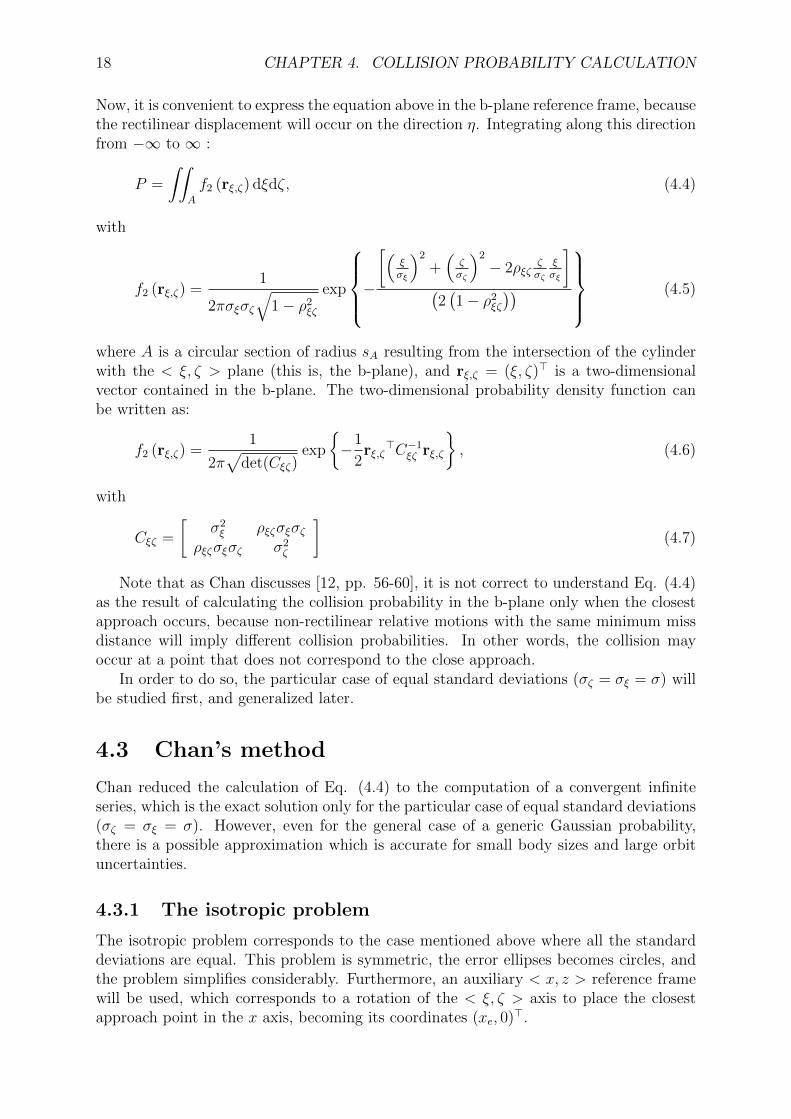
4.3.1 The isotropic problem
The isotropic problem corresponds to the case mentioned above where all the standarddeviations are equal. This problem is symmetric, the error ellipses becomes circles, andthe problem simplifies considerably. Furthermore, an auxiliary < x, z > reference framewill be used, which corresponds to a rotation of the < ξ, ζ > axis to place the closestapproach point in the x axis, becoming its coordinates (xe, 0)>.
4.3. CHAN’S METHOD 19
x
z
σ A
Figure 4.1: The isotropic problem.
The corresponding probability density function reads:
f2(x, z) =1
2πσ2exp
{−x
2 + z2
2σ2
}(4.8)
and the collision probability integral is:
P =
∫∫A
f2(x, z)dxdz (4.9)
where A is a circle centered in (xp, zp) = (xe, 0) of radius sA. The origin of the probabilitydensity function and the integration region may be swapped without altering the resultof the integral, resulting in:
P =1
2πσ2
∫∫A0
exp
{−(x− xe)2 + z2
2σ2
}dxdz (4.10)
being A0 the same circular region as before, but centered in the origin of < x, z >. Theequation above may be reduce to the an integral in only one variable:
fR(r) =r
σ2exp
{−r
2 + x2e2σ2
}I0
(rxeσ2
), (4.11a)
P =
∫ sA
0
fR(r)dr (4.11b)
where fR is the Rician probability density function, and I0 is the modified Bessel functionof the first kind of order zero.
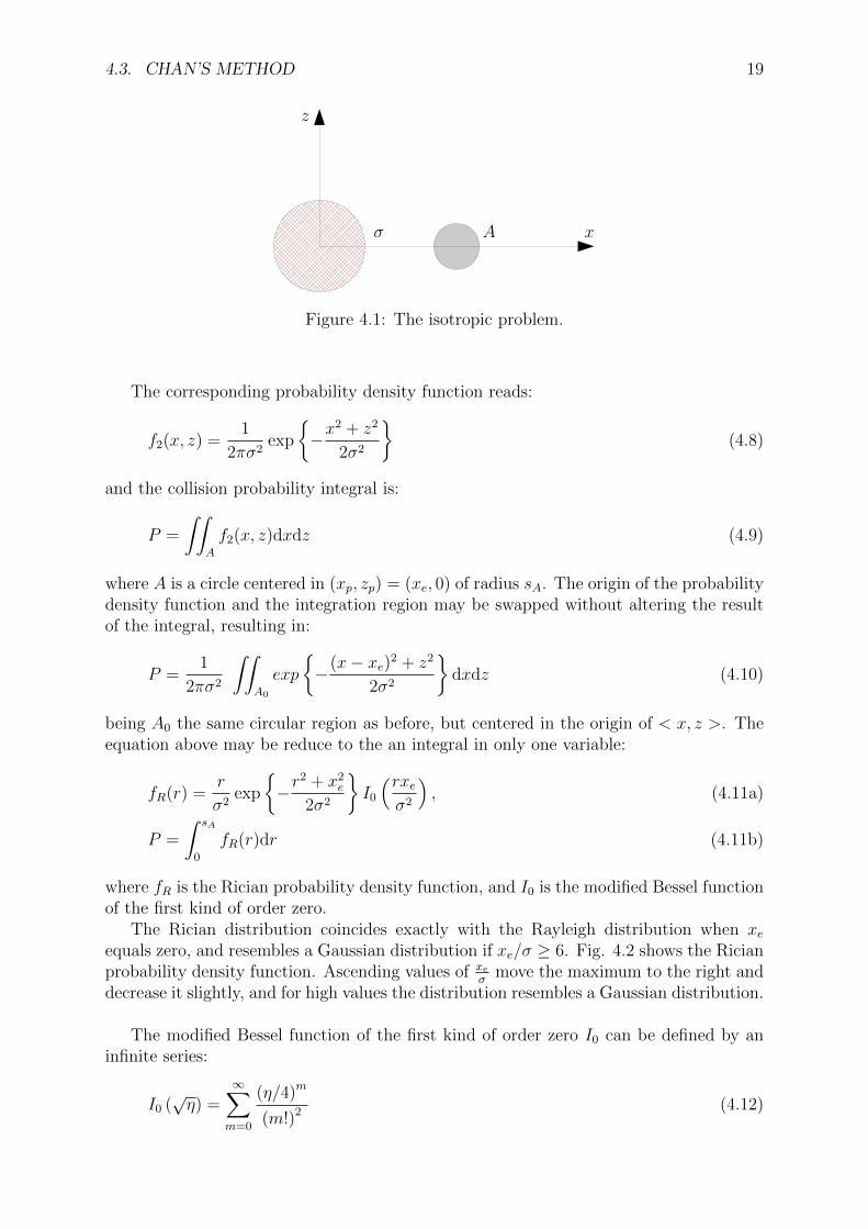
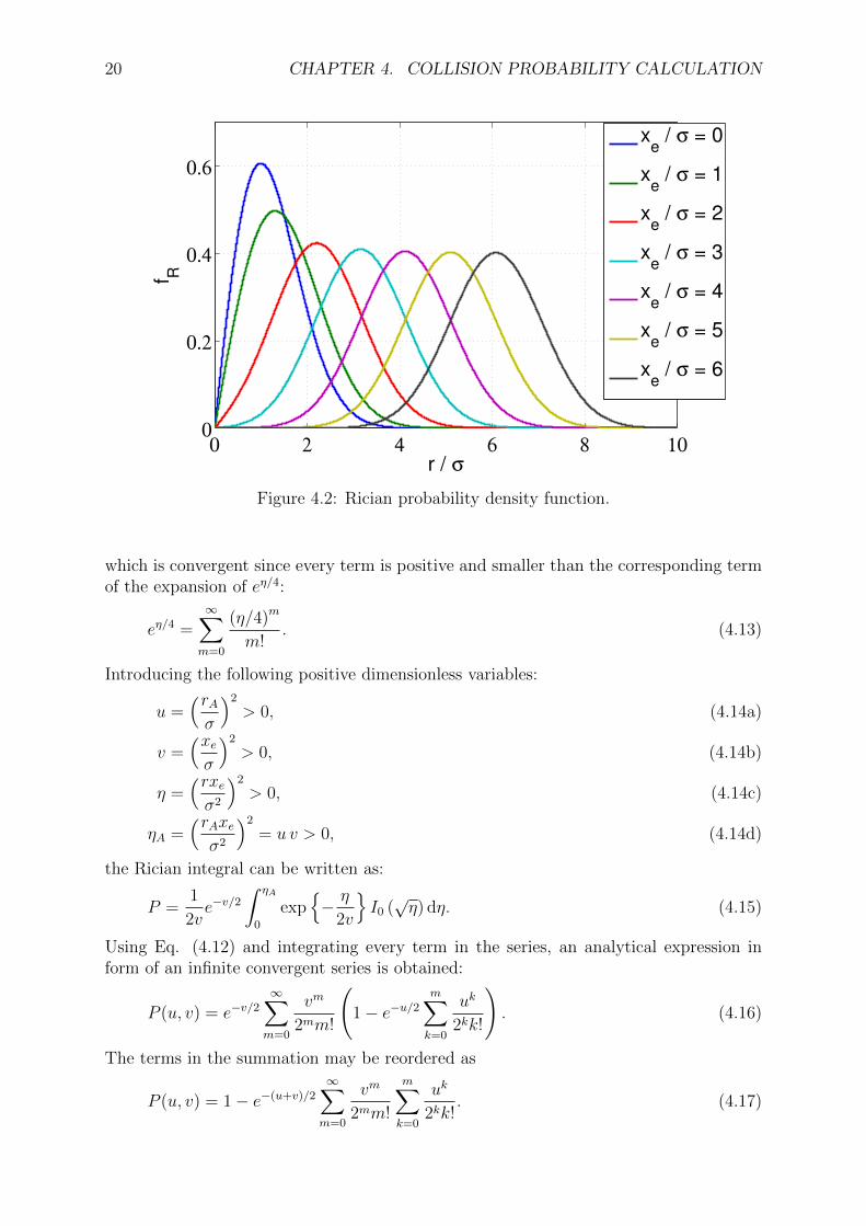
The Rician distribution coincides exactly with the Rayleigh distribution when xeequals zero, and resembles a Gaussian distribution if xe/σ ≥ 6. Fig. 4.2 shows the Ricianprobability density function. Ascending values of xe
σmove the maximum to the right and
decrease it slightly, and for high values the distribution resembles a Gaussian distribution.
The modified Bessel function of the first kind of order zero I0 can be defined by aninfinite series:
I0 (√η) =
∞∑m=0
(η/4)m
(m!)2(4.12)
20 CHAPTER 4. COLLISION PROBABILITY CALCULATION
0 2 4 6 8 100
0.2
0.4
0.6
r / σ
f R
xe / σ = 0
xe / σ = 1
xe / σ = 2
xe / σ = 3
xe / σ = 4
xe / σ = 5
xe / σ = 6
Figure 4.2: Rician probability density function.
which is convergent since every term is positive and smaller than the corresponding termof the expansion of eη/4:
eη/4 =∞∑m=0
(η/4)m
m!. (4.13)
Introducing the following positive dimensionless variables:
u =(rAσ
)2> 0, (4.14a)
v =(xeσ
)2> 0, (4.14b)
η =(rxeσ2
)2> 0, (4.14c)
ηA =(rAxeσ2
)2= u v > 0, (4.14d)
the Rician integral can be written as:
P =1
2ve−v/2
∫ ηA
0
exp{− η
2v
}I0 (√η) dη. (4.15)
Using Eq. (4.12) and integrating every term in the series, an analytical expression inform of an infinite convergent series is obtained:
P (u, v) = e−v/2∞∑m=0
vm
2mm!
(1− e−u/2
m∑k=0
uk
2kk!
). (4.16)
The terms in the summation may be reordered as
P (u, v) = 1− e−(u+v)/2∞∑m=0
vm
2mm!
m∑k=0
uk
2kk!. (4.17)
4.3. CHAN’S METHOD 21
To calculate the infinite series, it is convenient to do it recursively, because the factorialsand potential terms grow rapidly and may cause a loss of accuracy when surpassing themachine precision. To do so, the Rician integral is written as:
P (u, v) = e−v/2∞∑m=0
tm − e−(u+v)/2∞∑m=0
tmSm (4.18)
where tm, Sm and an auxiliary variable sm are defined as:
t0 = 1, s0 = 1, S0 = 1
tm = v2mtm−1, sm = u
2msm−1, Sm = Sm−1 + sm m = 1, 2, . . .
(4.19)
Note that even though Eq. (4.16) converges analytically, there may be numericalissues since in the parenthesis there are small terms subtracting to the unity. Whenthose terms are smaller than approximately 10−16 and the calculations are being made ina double precision machine, the successive decreasing terms will be part of the round-offerror, and the series may fail to converge numerically. By the same reason, round-offerror may cause incorrect results even when using the recursive algorithm for calculatingthe Rician integral: In Eq. (4.18), two decreasing terms are being subtracted, and mayhit the machine precision at different times, even to the point of returning a negativeresult. Consequently, the maximum value of m must be bounded. Chan proposes thefollowing criteria [12, page 74]:
• m = 3 for u ≤ 0.01 or v ≤ 1
• m = 10 for 0.01 < u ≤ 1 or 1 < v ≤ 9
• m = 20 for 1 < u ≤ 25 or 9 < v ≤ 25
• m = 60 otherwise
which as Chan states, provides good accuracy for the majority of the real mission sce-narios.
Since the Bessel function of the first kind of order zero is bounded by an exponential,a coarse error upper bound when truncating the infinite series may be obtained. Notethat what is being discussed here is the truncation error, not the round-off error discussedabove. From Eq. (4.12):
I0 (√η) =
N−1∑m=0
(η/4)m
(m!)2+RN (η) , (4.20)
where RN contains all the terms not considered in our approximation of I0. Note thatthe number of terms included in RN is infinite. However, since I0 is a convergent series,RN also converges:
0 < RN (η) <(η/4)N
(N !)2
∞∑k=0
(η/4)k
(k!)2<
(η/4)N
(N !)2e(η/4) (4.21)
Then, introducing RN in the probability integral (Eq. (4.15)), we can calculate theerror bound TN :
TN <1
2ve−v/2
∫ ηA
0
exp{− η
2v
}RN(η)dη (4.22)
22 CHAPTER 4. COLLISION PROBABILITY CALCULATION
This equation may be integrated exactly. However, since η < ηA in the whole integrationdomain, a simpler bound is obtained replacing η by ηA:
0 < TN <1
2ve−v/2
∫ ηA
0
exp{−ηA
2v
}RN(ηA)dη (4.23)
which is easily integrated. Recalling ηA = u v, the bounds for the truncation error read:
0 < TN <u
2
(u v4
)N(N !)2
exp{u v
4− v
2
}(4.24)
For large values of N , it may difficult to evaluate numerically this bound. For example,using a 64 bits version of Matlab 2013, calculating N ! for N > 170 returns infinite. Forthese cases, taking logarithms on both sides of the equation and using the Stirling’sapproximation for the factorial function:
ln (TN) = ln(u
2
)+u v
4− v
2+N ln
(u v4
)− 2 (N ln (N)−N) (4.25)
Note that this error bound is very conservative: it has been constructed using anexponential function as an upper bound. This means that for large values of the param-eters, it provides a huge bound. In addition, for u > 1, the exponential term will growand may return a value greater than 1, the maximum possible probability.
4.3.2 The general case
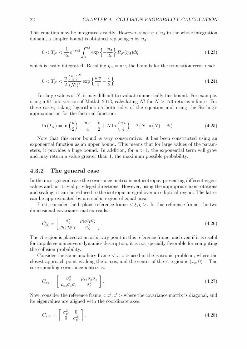
In the most general case the covariance matrix is not isotropic, presenting different eigen-values and not trivial privileged directions. However, using the appropriate axis rotationsand scaling, it can be reduced to the isotropic integral over an elliptical region. The lattercan be approximated by a circular region of equal area.
First, consider the b-plane reference frame < ξ, ζ >. In this reference frame, the twodimensional covariance matrix reads:
Cξζ =
[σ2ξ ρξζσξσζ
ρξζσξσζ σ2ζ
]. (4.26)
The A region is placed at an arbitrary point in this reference frame, and even if it is usefulfor impulsive maneuvers dynamics description, it is not specially favorable for computingthe collision probability.
Consider the same auxiliary frame < x, z > used in the isotropic problem , where theclosest approach point is along the x axis, and the center of the A region is (xe, 0)>. Thecorresponding covariance matrix is:
Cxz =
[σ2x ρxzσxσz
ρxzσxσz σ2z
]. (4.27)
Now, consider the reference frame < x′, z′ > where the covariance matrix is diagonal, andits eigenvalues are aligned with the coordinate axes:
Cx′z′ =
[σ2x′ 00 σ2
z′
]. (4.28)
4.3. CHAN’S METHOD 23
This reference frame is obtained by a clockwise rotation of the < x, z > reference frameby an angle θ such that:
θ =1
2tan−1
(2ρxzσxσzσ2x − σ2
z
). (4.29)
The circular region A becomes another circular region A′ of the same radius, centered in(xp′ , zp′)
> = (xe cos θ,−xe sin θ)>.An useful relation involving θ and the center of the region A′ mentioned above is:
cos θ =
xp′√x2p′ + z2p′
. (4.30)
x
z
A,A′
θ
x′
ξz′
ζ
σx′σz′
Figure 4.3: The general case.
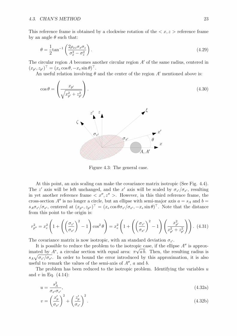
At this point, an axis scaling can make the covariance matrix isotropic (See Fig. 4.4).The z′ axis will be left unchanged, and the x′ axis will be scaled by σz′/σx′ , resultingin yet another reference frame < x′′, z′′ >. However, in this third reference frame, thecross-section A′′ is no longer a circle, but an ellipse with semi-major axis a = sA and b =sAσz′/σx′ , centered at (xp′′ , zp′′)
> = (xe cos θσz′/σx′ ,−xe sin θ)>. Note that the distancefrom this point to the origin is:
r2p′′ = x2e
(1 +
((σz′
σx′
)2
− 1
)cos2 θ
)= x2e
(1 +
((σz′
σx′
)2
− 1
)(x2p′
x2p′ + z2p′
)). (4.31)
The covariance matrix is now isotropic, with an standard deviation σz′ .It is possible to reduce the problem to the isotropic case, if the ellipse A′′ is approx-
imated by A∗, a circular section with equal area: π√a b. Then, the resulting radius is
sA√σz′/σx′ . In order to bound the error introduced by this approximation, it is also
useful to remark the values of the semi-axis of A′′, a and b.The problem has been reduced to the isotropic problem. Identifying the variables u
and v in Eq. (4.14):
u =s2A
σx′σz′, (4.32a)
v =
(x′pσx′
)2
+
(z′pσz′
)2
. (4.32b)
24 CHAPTER 4. COLLISION PROBABILITY CALCULATION
x
z
A′′, A∗
x′ ≡ x′′
z′ ≡ z′′
Figure 4.4: The general case. Axis scaling.
It is possible to write the equation above in a more general way. In the first place,note that det (Cx′z′) = σ2
x′σ2z′ . Since the absolute value of the determinant of a matrix
is invariant, then we can rewrite u using the covariance matrix in any reference frame.Secondly, v can be defined as the quadratic form of (xp′ , zp′)
> with an associated matrixC−1x′z′ . Then the same quadratic form in any other reference frame will also return thesame value of v. Using these two results, Eq. (4.32) can be expressed in the b-planereference frame:
u =r2A√
detCξζ=
r2A
σξσζ√
1− ρ2ξζ, (4.33a)
v = rξ,ζ>C−1ξζ rξ,ζ = r>Q∗r, (4.33b)
which are to be introduced in Eq. (4.16). The Q∗ matrix is built from the elements ofC−1ξζ , inserting 0 in the second row and column, corresponding to the η coordinate:
Q∗ =1
1− ρ2ξζ
1σ2ξ
0 − ρξζσξσζ
0 0 0− ρξζσξσζ
0 1σ2ζ
(4.34)
The equation above has an important implication: the collision probability is constantwhen the center of the combined area lays on constant error ellipses.
Only one things remains to be done: when replacing the ellipse A′′ by the circularregion A∗, what error is being introduced? To answer this question, the following boundwill be calculated: let A− and A+ be the circular regions tangent to A′′, such that A−is completely inside it, and A+ completely outside. The actual probability must bebounded by the probabilities calculated using A− and A+. The value v is not affected bythe approximation, and the value to be used is the same as the previous case.
The radius of this bounding circular section is, using the value of the semi-major axisof the elliptical section A′′:
u− =s2Aσ2max
, (4.35a)
u+ =s2Aσ2min
, (4.35b)
4.4. OTHER METHODS 25
where σmax and σmin are the maximum and the minimal value of (σx′ , σz′ . However, thesevalues squared are the eigenvalues of the covariance matrix Cx′z′ , so they can be rewrittenin a more general way:
σ2max,min =
TrC
2±
√(TrC
2
)2
− detC (4.36)
with the sign + for σmax, and − for σmin. This expression is valid for any matrix C,since the trace and the determinant are invariants. The particular expression using theb-plane reference frame reads:
σ2max,min =
σ2ξ + σ2
ζ
2±
√(σ2ξ + σ2
ζ
2
)2
− σ2ξσ
2ζ
(1− ρ2ξζ
)(4.37)
which finally allows bounding the result.
4.4 Other methods
While the analytical formulation developed by Chan is powerful and allows inferringinteresting properties like the constant probability curves with constant v, it has two maindrawbacks. The first one is the approximation done when replacing the elliptical combinedcross-section by a same area circular contour: this is in general a good approximation butmay fail for large values of u. The second problem we may face is when implementingthe infinite (analytically) convergent series, which may fail to converge to the true valuebecause of the truncation (finite maximum value of m) and round-off errors (because ofthe floating-point arithmetic used in a computer).
It may be interesting to explore other methods more precise, even if they are compu-tationally more expensive. A detailed comparison between these methods was publishedby Alfano [26].
4.4.1 Foster’s Method
Foster developed in 1992 his method used by NASA for analyzing the hazard of spacedebris on the International Space Station [21]. It is based on a two-dimensional integralof the collision probability function on the circular domain corresponding to the sphericalenvelop with radii the sum of the radius of the two objects. The calculation of the collisionprobability is reduced to the calculation of the following integral:
P =1
2πσx′σz′exp
{− x2e
2
[(sinϕ
σx′
)2
+
(cosϕ
σz′
)2]}
∫ sA
0
r
∫ 2π
0
exp
{− r2
2
[(sinα
σx′
)2
+
(cosα
σz′
)2]
+ rxe
[(sinα sinϕ
σ2x′
)+
(cosα cosϕ
σ2z′
)]}dαdr.
(4.38)
In the above equation, ϕ is the angle between the radius vector of the center of thecircular domain and the z′ axis, and corresponds to π/2 − θ (see Eq. (4.29)). He chosean angular discretization of 0.5 deg and a radial discretization of sA/12.
26 CHAPTER 4. COLLISION PROBABILITY CALCULATION
4.4.2 Patera’s Method
Patera developed an alternative way of evaluating Eq. (4.38), and reduced the problemto a line integral [22].
As was done developing the general case of Chan’s Method, a series of rotations andscaling are performed to transform the probability density function into an isotropic dis-tribution (see Fig. 4.4 for reference). Consequently the combined body contour becomesan ellipse. The resulting probability density function was integrated by Chan using anapproximate domain of integration, performing a first integral in the tangential directionas an infinite series, which can be integrated a second time analytically. Patera pro-poses instead a radial integration, which reduces the problem to a line integral over thedeformed body-section in the counter-clockwise direction.
If the origin is not contained in the hard-body, the collision probability integral reads
P = − 1
2π
∮ellipse
exp{−αr2
}dθ, (4.39)
and if the origin lays inside the hard-body, the equation above becomes
P = 1− 1
2π
∮ellipse
exp{−αr2
}dθ. (4.40)
In the equations above, α is a function of the combined covariance in the b-plane refer-ence frame, resulting from transforming the probability density function into an isotropicdistribution in the same fashion as Chan. The interested reader is referred to [22].
4.4.3 Alfano’s method
Alfano [23] obtained a first integral of the direct integration of the 2-d density proba-bility function using the error function. Then, the resulting one-dimensional integral isdiscretized, providing an analytic expression for calculating the error probability.
The probability integral expressed in the < X ′, Z ′ > reference frame (where thecovariance matrix is diagonal) is:
P =1
2πσx′σz′
sA∫−sA
√s2A−x′2∫
−√s2A−x′2
exp
{−1
2
((x′ + x′eσx′
)2
+
(z′ + z′eσz′
)2)}
dz′
dx′. (4.41)
Where (x′e, z′e) are the coordinates of the secondary body. The equation above may be
integrated once to become:
P =1√
8πσx′
sA∫−sA
(erf
(z′e +
√s2A − x′2√2σz′
)+ erf
(−z′e +
√s2A − x′2√
2σz′
))
exp
(− (x′ + x′e)
2
2σ2x′
)dx′.
(4.42)
4.4. OTHER METHODS 27
Alfano used at this point a n-series expansion for the equation above:
P =sA√
2πσx′n
n∑i=0
[erf
z′e + 2sA
√(n−i)in√
2σz′
+
erf
−z′e + 2sA
√(n−i)in√
2σz′
exp
(−(sA
2i−nn
+ x′e)2
2σ2x′
)] (4.43)
where the integration variable x′ has been replaced by
x′ = sA2i− nn
(4.44)
and
dx′ =2sAn. (4.45)
Using the Simpson’s one-third rule, and reordering the series, he obtained an alternatem-series expansion. By setting
dx′ =sA2m
(4.46)
and
z′ (x′) =√s2A − x′2 (4.47)
the calculation of the collision probability reduces to:
P =dx′
6√
2πσx′(meven +modd +m0) . (4.48)
The odd-order term reads
modd = 4m∑i=1
[(erf
(z′e + z′(x′)√
2σz′
)− erf
(z′e − z′(x′)√
2σz′
))(
exp
(− (x′ + x′e)
2
2σ2x′
)+ exp
(− (x′ − x′e)
2
2σ2x′
))] (4.49)
where the x′ of the odd-order term series is defined as
x′ = (2i− 1) dx′ − sA (4.50)
The even-order term reads:
meven =2m−1∑i=1
[(erf
(z′e + z′(x′)√
2σz′
)− erf
(z′e − z′(x′)√
2σz′
))(
exp
(− (x′ + x′e)
2
2σ2x′
)+ exp
(− (x′ − x′e)
2
2σ2x′
))]
+ 2
(erf
(z′e + sA√
2σz′
)− erf
(z′e − sA√
2σz′
))(exp
(−x′2e2σ2
x′
))(4.51)
28 CHAPTER 4. COLLISION PROBABILITY CALCULATION
where the x′ of the even-term series is defined as
x′ = 2idx′ − sA (4.52)
The zeroth term was heuristically adjusted, and Alfano proposed
m0 = 2
(erf
(z′e + z′(x′)√
2σz′
)− erf
(z′e − z′(x′)√
2σz′
))(
exp
(− (x′ + x′e)
2
2σ2x′
)+ exp
(− (x′ − x′e)
2
2σ2x′
)) (4.53)
where the x′ of the zeroth term is defined as
x′ = 0.015dx′ − sA (4.54)
The accuracy of the collision probability (Eq. 4.48) depends on the value of m. Alfanoset:
m = int
5sA
min(σx′ , σz′ ,
√x′2e + z′2e
) (4.55)
where int is the integer part function. Alfano also defined a lower bound of 10 and anupper bound of 50, which provides sufficient accuracy for real-mission scenarios.
4.4.4 Akella and Alfriend’s method
Akella and Alfriend were motivated by Foster method to develop their own method [24].Their method hinges on the integration of Eq. (4.3) on time, using the relative velocityVr, since dη ' Vrdt:
P =
∫ ∞−∞
Vr√(2π)3 |C|
∫A
exp
{−1
2r>C−1r
}dξdζdt. (4.56)
Note that this approach reduces to Eq. (4.4) if the short-term encounter hypothesis holds.
Chapter 5
Collision avoidance maneuveroptimization
5.1 Introduction
Collision avoidance maneuvers are performed several times in the lifetime of a satellite,consumes an important amount of fuel and may hinder the mission. Then, it is importantto design optimal maneuvers in order to reduce the fuel budget alloted for these situations.
Typical collision avoidance maneuver optimization algorithms rely on parametricsearches [7], gradient methods [12, Chapter 7], or other methods like Genetic Algorithms[9] or Multi-Objective Particle Swarm Optimizers [10].
However, using the impulsive maneuver linearization (Section 2.4), it is possible tosolve the optimization problem in a more efficient manner, allowing to write the objec-tive function and the constraints of the problem as quadratic forms of the optimizationvariable. This idea was already proposed by Conway [29] in the context of asteroid orbitmodification, and can be applied to the particular problem of satellite collision avoidancemaneuvers too.
The main reference for this chapter is Convex Optimization by Boyd et. al [30]
5.2 Some notes on optimization theory
5.2.1 Unconstrained optimization
Let f : R 7→ R be a real function of the real variable x. A necessary and sufficientcondition for f(x) to have a local minimum in the point x0 is:
f(x0 + δx) > f(x0), ∀δx. (5.1)
A necessary condition for the point x0 to be an extrema of f is, provided that f isdifferentiable:
d f
dx
∣∣∣∣x=x0
= 0. (5.2)
To distinguish between minimum and maximum points, the second derivative must becalculated. A positive sign will result in a local minimum of the function:
d2f
dx2
∣∣∣∣x=x0
> 0. (5.3)
29
30 CHAPTER 5. COLLISION AVOIDANCE MANEUVER OPTIMIZATION
Note that a negative sign will mean a local maxima because minimizing f(x) is equivalentto maximizing −f(x). If the second derivative is exactly zero, higher order derivativesmust be calculated, and if the first non-zero derivative is even, the point will not beneither a maximum or a minimum, but an inflection point (for example, the functionf(x) = x3 has null first and second derivatives in x = 0, but since the third derivative ispositive it is an inflection point).
This result can be generalized to higher dimensions. Now let f : Rn 7→ R take realvectors as input, and return a real scalar value. The necessary and sufficient conditionfor optimality becomes:
f(x0 + δx) > f(x0), ∀δx. (5.4)
Eqs. (5.2) and (5.3) now read:
∇f |x=x0 = 0, (5.5)
∇2f |x=x0 ∈ Sn++, (5.6)
where ∇f is denotes the gradient of the function f , ∇2f the Hessian of the function f ,and Sn++ is the set of symmetric positive definite matrices.
5.2.2 Constrained optimization
Let us consider the following problem:
minimize f0(x)subject to fi(x) ≤ 0, i = 1, . . . ,m,
hi(x) = 0, i = 1, . . . , p,(5.7)
with the optimization variable x ∈ Rn. Introducing the Lagrange multipliers or dualvariables λi and µi associated to fi and hi respectively, the Lagrangian function L :Rn × Rm × Rp 7→ R is defined as:
L(x, λ, µ) = f0(x) +m∑i=1
λifi(x) +
p∑i=1
νihi(x). (5.8)
Then, the Lagrange dual function, or simply dual function g : Rm×Rp 7→ R is definedas the minimum of the Lagrangian function over x:
g(λ, ν) = inf L(x, λ, ν). (5.9)
The dual function is bounded above by the optimal value p∗ of the problem (p stands forprimal problem):
g(λ, ν) ≤ p∗. (5.10)
This property leads to the Lagrange dual problem:
minimize g(λ, ν)subject to λ ≥ 0,
(5.11)
5.3. DIRECT IMPACT 31
where λ cannot be negative in order to satisfy the inequality constraints. This is, theLagrange dual problem focus on searching the maximum lower bound d∗ (d stands fordual problem). It is unclear that d∗ and p∗ coincide, and in fact in the general case theydo not. This is referred to as weak duality:
d∗ ≤ p∗. (5.12)
The difference between these two values is called duality gapIf the duality gap is exactly 0, strong duality is obtained:
d∗ = p∗. (5.13)
Boyd showed that strong duality holds for Quadratic Constrained Quadratic Programproblems (QCQP) [30, pp. 227-228]. This result will be enough for this work, but moreresults are available in the reference.
It is possible to obtain a necessary condition for optimality in the problem defined byEq. (5.7). Let x∗ and (λ∗, ν∗) be the primal and dual optimal values, with zero dualitygap. Since x∗ minimizes the Lagrangian function, its gradient must vanish:
∇f0(x∗) +m∑i=1
λ∗i∇fi(x∗) +
p∑i=1
ν∗i∇hi(x∗) = 0, (5.14)
and from the equation above the Karush-Kuhn-Tucker (KKT) conditions are obtained
fi(x∗) ≥ 0, i = 1, . . . ,m (5.15a)
hi(x∗) = 0, i = 1, . . . , p (5.15b)
λ∗i ≥ 0, i = 1, . . . ,m (5.15c)
λ∗i fi(x∗) = 0, i = 1, . . . ,m (5.15d)
∇f0(x∗) +m∑i=1
λ∗i∇fi(x∗) +
p∑i=1
ν∗i∇hi(x∗) = 0. (5.15e)
Note that the KKT conditions are a generalization of the method of Lagrange Multipli-ers to include inequality constraints, or equivalently, the method of Lagrange Multiplierscorresponds to a particular case of the KKT conditions with m = 0.
Additionally, in a Quadratic Constrained Quadratic Program maximization problemwith a positive definite matrix defining the quadratic forms, the optimal value will beattained in the boundary defined by the constraints, so the normal method of LagrangeMultipliers can be used.
5.3 Direct Impact
In this section, the simplified case of a conjunction that leads to a zero minimum distancebetween the nominal orbits is studied. Such a scenario is not realistic, since the probabilityof this event is negligible, but is the basis for the general case of non-intersecting objects.Note that a even in a Direct Impact case, a collision is not certain: the uncertainty ofthe orbits allows the two objects not to impact to each other.
There are two different kind of interesting maneuvers: those that maximize the missdistance, and those that minimize the collision probability. For both maneuvers, a max-imum fuel consumption will be alloted, expressed as a maximum impulse size ∆V0.
32 CHAPTER 5. COLLISION AVOIDANCE MANEUVER OPTIMIZATION
5.3.1 Maximum miss distance
The miss distance δr is easily expressed in the b plane reference frame, since according tothe short term encounter hypothesis, the relative motion becomes a straight line in the ηdirection, and the maximum approach point will be contained in the < ξ, ζ > plane. Themiss distance is a poor choice of objective function for this optimization problem, becauseit is a fairly complicated function. Instead, it is more convenient to use the squared missdistance as the objective function
Jr(∆V) = δr2max = ξ2 + ζ2 (5.16)
because it can be written as a quadratic form:
Jr(∆V) = r>Qr, (5.17)
with
Q =
1 0 00 0 00 0 1
. (5.18)
Note that a solution for the squared miss distance optimization problem will also be asolution for the miss distance one. Using the linear impulsive maneuver formula (Eq.2.12), the objective function becomes:
Jr(∆V) = ∆V>A∆V, (5.19)
where the A is a semi-positive definite matrix defined as
A = M>QM. (5.20)
The constraint for the optimization problem is easily expressed using the norm of theapplied impulse:
f(∆V) = ∆V>∆V −∆V 20 ≥ 0. (5.21)
Note that the maximum of Eq. (5.19) is always attained in the boundary, so in theequation above the inequality may be changed by an equals sign.
The optimization problem is written then as
maximize Jr(∆V) = ∆V>A∆Vsubject to f(∆V) = ∆V>∆V −∆V 2
0 = 0(5.22)
This problem is easily reduced to an eigenvalues and eigenvectors problem. The La-grangian function for this problem is constructed as:
L(∆V, λ) = ∆V>A∆V − λ(∆V>∆V −∆V 2
0
). (5.23)
The gradient of the Lagrangian function with respect of the applied impulse reads:
∇L = 2A∆V − 2λ∆V. (5.24)
5.3. DIRECT IMPACT 33
According to the KKT conditions 5.15, the gradient must vanish at the solutions of theoptimization problem. This condition leads to
A∆V = λ∆V, (5.25)
which is a eigenvalues and eigenvectors problem of the matrix A. It is easily solvedobtaining λi ≥ 0 the eigenvalues of matrix A in descending order (λ1 ≥ λ2 ≥ λ3 = 0) andsi the corresponding eigenvectors with i = 1, 2, 3. Because of the rank deficiency inducedby the Q matrix, λ3 = 0 at all times. The optimal solution will correspond to
λopt =λ1, (5.26a)
∆Vopt =∆V0s1, (5.26b)
and using the constraint f(∆V), it is possible to write the squared maximum missdistance as:
Jr,opt = δr2max = ∆V 20 λ1. (5.27)
Note that the solution obtained here is double: reversing the direction of the optimalimpulse is a solution as optimal as the previous one. One of the maneuvers is progradeand adds energy to the orbit, while the other is retrograde and subtracts energy. No moreoptimal solutions exist for this problem.
5.3.2 Minimum collision probability
Intuitively one may think that the miss distance optimization must minimize the collisionprobability, since separating as much as possible the objects should make a collisionless probable. However this is a fallacious argument, and a simple counterexample isimmediate: suppose that the relative motion is perfectly determined in one direction(this is, restricted to a plane). If the relative distance perpendicular to the plane ofmotion is greater than the combined radius of the objects, the collision probability will beexactly 0, and consequently a collision avoidance maneuver that minimizes the collisionprobability will try to increase that distance. On the other hand, the maneuver thatmaximizes the miss distance will try to separate the objects in the three dimensions ofspace. Consequently, the method developed above must be modified to take into accountthe uncertainty of the orbits.
A first naive idea for formulating the minimization of the collision probability with amaximum alloted fuel consumption is:
minimize P (∆V)subject to f(∆V) = ∆V>∆V −∆V 2
0 = 0(5.28)
which has an important drawback compared to the previous problem: in this case, theobjective function is a strongly non-linear function of ∆V. An easy method for computingthe solution does not exist, and little can be said about the possible number of solutions.Additionally, it is not possible to discern if a solution is a global or local minima unlessthe whole domain of the optimization problem is swept. Numerical methods exist forsolving the problem above, such as the steepest descent method [30, pp. 457-484] orinterior-point methods [30, pp. 561-630], but do not guarantee global optimality. Since
34 CHAPTER 5. COLLISION AVOIDANCE MANEUVER OPTIMIZATION
the velocity is a three dimensional vector, and using the constraint f(∆V) = 0, a two-dimensional parametric search may be employed, testing all the possible maneuvers andfinding the optimal solution.
However, an alternative strategy is possible. Note that the collision probability cal-culated using Chan’s method as formulated in Eq. (4.16) is constant for fixed values ofv, and decreases with it roughly exponentially. Then, it is possible to define v as theobjective function of a maximization optimization problem:
maximize Jp(∆V) = ∆r>Q∗∆rsubject to f(∆V) = ∆V>∆V −∆V 2
0 = 0(5.29)
where Q∗ is the matrix defined previously in Eq. (4.34). Now, the objective function is aquadratic function of the position in the b plane, in the same fashion as in the previousoptimization problem, but with Q∗ as associated matrix instead of Q. This is, the twoproblems are mathematically equivalent, and any method that solves one of the problemswill solved the other one as well.
Following the same steps as in the previous section, the objective function becomes
Jp(∆V) = ∆V>A∗∆V, (5.30)
where
A∗ = M>Q∗M. (5.31)
It is already known that this problem is reduced to calculating the eigenvalues λ∗i andeigenvectors s∗i of the matrix A∗, with i = 1, 2, 3 and λ∗1 ≥ λ∗2 ≥ λ∗3 = 0. The optimalimpulse direction is along the s∗1 vector:
∆Vopt = ∆V0s∗1, (5.32)
The resulting parameter v for calculating the collision probability is
Jp,opt = vopt = ∆V 20 λ∗1 (5.33)
5.3.3 Discussion
Up to this point, a method for either maximizing miss distance or minimizing collisionprobability for the case of a direct impact of the nominal orbits has been presented. Inthis section, some properties and observations are listed.
In the first place, note the computational efficiency of the method: for each maneuveranticipation angle ∆θ, the matrix M is calculated using the impulsive maneuver formulas,and then the matrix A or A∗ is computed. Finally, only the eigenvalues and eigenvectorsproblem remains, and since it is a three dimensional matrix it has a closed form solution(however a general numerical algorithm may be preferable to prevent singularities fromhampering the method).
Secondly, since the two optimization problems have been proved to be equivalent, theimplementation of both problems in a single computer code can be reduced to a singleroutine that takes as input variable the matrix Q or Q∗ and computes the rest of theoperations in the same way.
Finally, note that the maneuver orientation angles σ and γ are independent of theapplied impulse magnitude in a direct impact scenario. This has a clear application,when a certain threshold of collision probability is to be achieved: the problem may besolved with a generic ∆V0 to obtain the maneuver orientation angles, and the magnitudescale a posteriori to ensure the required collision probability.
5.4. NON-DIRECT IMPACT 35
5.4 Non-Direct Impact
A Non-Direct Impact may be regarded as a generalization of the Direct Impact when thedistance at the closest approach epoch is not zero. By definition of the b plane, the ηcoordinate of the closest approach distance will vanish, but the other two componentsmay take any value. Then, the closest approach relative position re without maneuverreads:
re =
ξe0ζe
. (5.34)
Since the optimization of the miss distance is equivalent to the minimization of thecollision probability replacing Q by Q∗, only the former problem will be studied.
5.4.1 Maximum miss distance
Let us recall the formulation for the maximization of the miss distance:
maximize Jr(∆V) = ∆r>Q∆rsubject to f(∆V) = ∆V>∆V −∆V 2
0 = 0(5.35)
Introducing the initial offset in the b plane position in the objective function and expand-ing the result, two additional terms appear:
δr2 = r>Qr = (re +M∆V)>Q (re +M∆V)
= ∆V>M>QM︸ ︷︷ ︸A
∆V + 2 re>QM︸ ︷︷ ︸
∆V0b>
∆V + re>Qre. (5.36)
In the above equation, the first term was already present in the Direct Impact formulation,but a linear term on ∆V and a constant term appear. The latter may be dropped toperform the optimization, but the linear term introduces additional complexity into theproblem. It is convenient to normalize the velocity impulse vector to reduce the problemto a standard form. To this end, a dimensionless vector u is introduced:
u = ∆V/∆V0 (5.37)
and after multiplying by the appropriate constants, the optimization problem is trans-formed into:
maximize Jr(u) = u>Au + 2b>u
subject to f(u) = u>u− 1 = 0(5.38)
This is a non-convex optimization problem that may be reduced to a convex-optimizationproblem [30, p. 229]. For this problem, the Lagrangian function is easily calculated:
L(u, λ) = u>Au + 2u>b− λ(u>u− 1
), (5.39)
which allows calculating the Lagrangian dual function, as the infimum of the Lagrangianfunction. The gradient of L with respect of u must be zero:
∇u = 2Au + 2b− 2λu = 0, (5.40)
36 CHAPTER 5. COLLISION AVOIDANCE MANEUVER OPTIMIZATION
which leads to
u = − (A− λI)† b (5.41)
where the dagger symbol † indicates the matrix pseudoinverse. Substituting into theLagrangian function:
g(λ) =
{−b> (A− λI)† b + λ, A− λI � 0, b ∈ R(A− λI)
∞ otherwise(5.42)
In the equation above, R is the range of the matrix. Since we are dealing with a QuadraticConstrained Quadratic Program problem (QCQP), the duality gap is zero and strongduality holds, which ensures that the dual optimal is equal to the primal optimal. Thedual problem reads:
minimize − b> (A− λI)† b + λ
subject to A− λI � 0, b ∈ R(A− λI)(5.43)
The problem can be simplified if the quadratic form in the objective function is calculatedin a basis where the matrix is diagonal (this is equivalent to diagonalizing the matrix Aand projecting the b vector accordingly). Because the zero eigenvalue is associated withthe η direction and b has a null projection over it, s3
>b = 0 in in this problem. Also, notethat the constraint is equivalent to λ ≥ λ1. With these advances, the problem becomes:
minimize(s1>b)2
λ− λ1+
(s2>b)2
λ− λ2+ λ
subject to λ ≥ λ1
(5.44)
which can be minimized easily using numerical methods on the only variable optimizationλ. If the solution is not on the boundary (λopt = λ1), the solution may be obtainedimposing the null derivative with respect of λ condition on the objective function:
F (λ) =
(s1>b
λ1 − λ
)2
+
(s2>b
λ2 − λ
)2
− 1 = 0,
λ ≥ λ1,
(5.45)
which is a non-linear equation that has no closed form solution and in general presents upto 4 different solutions, but after imposing the constraint on λ only one solution is possible(note that it may be a double solution in the case of λopt = λ1 being the solution). Tosolve it, the Newton’s Method will be used [31]. This iterative method starts with a guessλ(0) updates the solution descending in the gradient direction until some tolerances inthe function and the variable step size are fulfilled. Mathematically, suppose the methodhas already calculated λ(k). The next step will be, expanding in Taylor series:
F (λ(k+1)) = F (λ(k)) +∂F
∂λ
∣∣∣∣λ(k)
(λ(k+1) − λ(k)) + . . . = 0. (5.46)
The method seeks solving F (λ) = 0, so F (λ(k+1)) is set to 0 with the intention of obtaininga better value for λ. Solving for λ(k+1) − λ(k):
λ(k+1) − λ(k) = −F (λ(k))/ ∂F
∂λ
∣∣∣∣λ(k)
(5.47)
5.4. NON-DIRECT IMPACT 37
a better value is obtained provided that the method is converging, which will do if theinitial guess is close enough to the true value of λ. The method will stop if some tolerancesε1 and ε2 are satisfied:
λ(k) − λ(k−1)
λ(k)< ε1, (5.48a)
F(λ(k))< ε2. (5.48b)
The following initial guess is proposed. If s1>b = 0, then λ can be solved from the
equation: λ = λ2 + |s2>b| (if it is greater than λ1). If s1>b 6= 0, a bigger value may
be possible, so this is a lower bound. In the same way, if s2>b = 0, doing the same
operations λ ≥ λ1 + |s1>b|. Collecting both results, the initial guess will be:
λ(0) = max(λ1 + |s1>b|, λ2 + |s2>b|
). (5.49)
After this point, the curve is monotonically decreasing, so quadratic convergence is guar-anteed. In most cases this initial guess is so good that verifies the tolerances imposed
This is not the only possible method for solving Eq. (5.45): it is also possible to usefor example the slower, but more robust bisection method.
When the optimal solution λopt has been obtained, the optimal impulse can be calcu-lated using Eq. (5.41).
Note that in the case of the Non-Direct Impact, the optimal direction depends on themagnitude of the applied impulse magnitude ∆V0. This is justified analyzing Eq. (5.45),where the λi and si do not depend on ∆V0 because A does not depend either, but bdepends linearly on the impulse size: consequently, the solution of the equation λopt alsodepends on ∆V0.
As stated previously, if one was to minimize collision probability, the method describedhere still applies replacing Q by Q∗.
5.4.2 An implicit constraint
There is an interesting implicit constraint hidden in the Non-direct Impact optimizationproblem. It allows formulating an a priori property of the optimal impulse by onlyanalyzing the objective function of the optimization problem (Eq. 5.36).
Suppose a generic impulse ∆V (generic as we do not request it to be an optimalsolution) that satisfies
Jr(−∆V) > Jr(∆V), (5.50)
this is, changing ∆V by −∆V, an increase of the objective function is found: the selectedimpulse ∆V cannot be an optimum. Since only the linear term in Eq. (5.36) is affectedby this change, we can infer the existence of a half-space of non optimal solutions:
re>QM∆Vnon−opt < 0. (5.51)
Consequently, the optimal solution ∆Vopt must satisfy the following implicit constraint:
re>QM∆Vopt ≥ 0. (5.52)
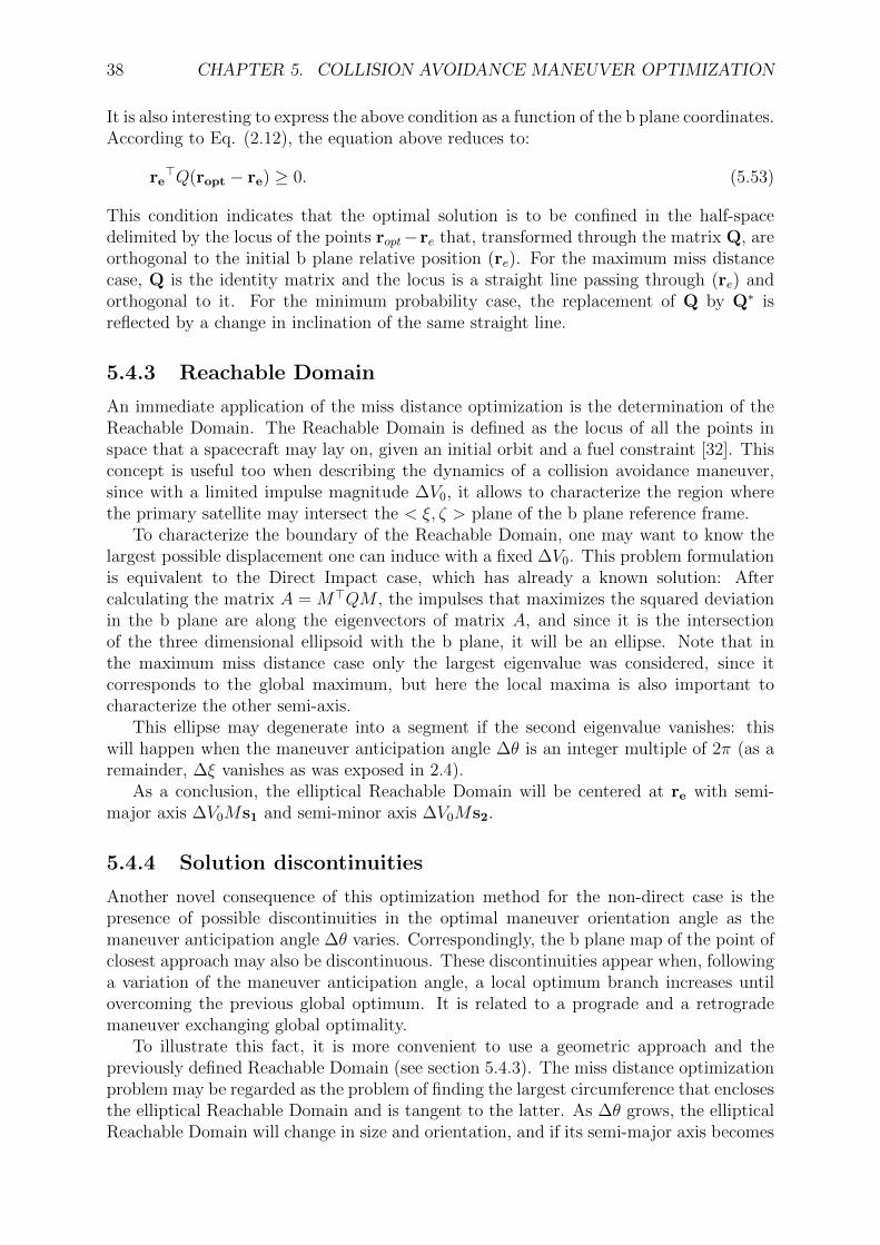
38 CHAPTER 5. COLLISION AVOIDANCE MANEUVER OPTIMIZATION
It is also interesting to express the above condition as a function of the b plane coordinates.According to Eq. (2.12), the equation above reduces to:
re>Q(ropt − re) ≥ 0. (5.53)
This condition indicates that the optimal solution is to be confined in the half-spacedelimited by the locus of the points ropt−re that, transformed through the matrix Q, areorthogonal to the initial b plane relative position (re). For the maximum miss distancecase, Q is the identity matrix and the locus is a straight line passing through (re) andorthogonal to it. For the minimum probability case, the replacement of Q by Q∗ isreflected by a change in inclination of the same straight line.
5.4.3 Reachable Domain
An immediate application of the miss distance optimization is the determination of theReachable Domain. The Reachable Domain is defined as the locus of all the points inspace that a spacecraft may lay on, given an initial orbit and a fuel constraint [32]. Thisconcept is useful too when describing the dynamics of a collision avoidance maneuver,since with a limited impulse magnitude ∆V0, it allows to characterize the region wherethe primary satellite may intersect the < ξ, ζ > plane of the b plane reference frame.
To characterize the boundary of the Reachable Domain, one may want to know thelargest possible displacement one can induce with a fixed ∆V0. This problem formulationis equivalent to the Direct Impact case, which has already a known solution: Aftercalculating the matrix A = M>QM , the impulses that maximizes the squared deviationin the b plane are along the eigenvectors of matrix A, and since it is the intersectionof the three dimensional ellipsoid with the b plane, it will be an ellipse. Note that inthe maximum miss distance case only the largest eigenvalue was considered, since itcorresponds to the global maximum, but here the local maxima is also important tocharacterize the other semi-axis.
This ellipse may degenerate into a segment if the second eigenvalue vanishes: thiswill happen when the maneuver anticipation angle ∆θ is an integer multiple of 2π (as aremainder, ∆ξ vanishes as was exposed in 2.4).
As a conclusion, the elliptical Reachable Domain will be centered at re with semi-major axis ∆V0Ms1 and semi-minor axis ∆V0Ms2.
5.4.4 Solution discontinuities
Another novel consequence of this optimization method for the non-direct case is thepresence of possible discontinuities in the optimal maneuver orientation angle as themaneuver anticipation angle ∆θ varies. Correspondingly, the b plane map of the point ofclosest approach may also be discontinuous. These discontinuities appear when, followinga variation of the maneuver anticipation angle, a local optimum branch increases untilovercoming the previous global optimum. It is related to a prograde and a retrogrademaneuver exchanging global optimality.
To illustrate this fact, it is more convenient to use a geometric approach and thepreviously defined Reachable Domain (see section 5.4.3). The miss distance optimizationproblem may be regarded as the problem of finding the largest circumference that enclosesthe elliptical Reachable Domain and is tangent to the latter. As ∆θ grows, the ellipticalReachable Domain will change in size and orientation, and if its semi-major axis becomes
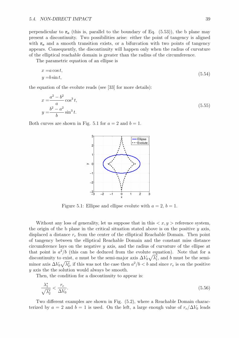
5.4. NON-DIRECT IMPACT 39
perpendicular to re (this is, parallel to the boundary of Eq. (5.53)), the b plane maypresent a discontinuity. Two possibilities arise: either the point of tangency is alignedwith re and a smooth transition exists, or a bifurcation with two points of tangencyappears. Consequently, the discontinuity will happen only when the radius of curvatureof the elliptical reachable domain is greater than the radius of the circumference.
The parametric equation of an ellipse is
x =a cos t,
y =b sin t,(5.54)
the equation of the evolute reads (see [33] for more details):
x =a2 − b2
acos3 t,
y =b2 − a2
bsin3 t.
(5.55)
Both curves are shown in Fig. 5.1 for a = 2 and b = 1.
−3 −2 −1 0 1 2 3−3
−2
−1
0
1
2
3
x
y
Ellipse
Evolute
Figure 5.1: Ellipse and ellipse evolute with a = 2, b = 1.
Without any loss of generality, let us suppose that in this < x, y > reference system,the origin of the b plane in the critical situation stated above is on the positive y axis,displaced a distance re from the center of the elliptical Reachable Domain. Then pointof tangency between the elliptical Reachable Domain and the constant miss distancecircumference lays on the negative y axis, and the radius of curvature of the ellipse atthat point is a2/b (this can be deduced from the evolute equation). Note that for adiscontinuity to exist, a must be the semi-major axis ∆V0
√λ∗1, and b must be the semi-
minor axis ∆V0√λ∗2, if this was not the case then a2/b < b and since re is on the positive
y axis the the solution would always be smooth.Then, the condition for a discontinuity to appear is:
λ∗1√λ∗2
<re
∆V0. (5.56)
Two different examples are shown in Fig. (5.2), where a Reachable Domain charac-terized by a = 2 and b = 1 is used. On the left, a large enough value of re/∆V0 leads
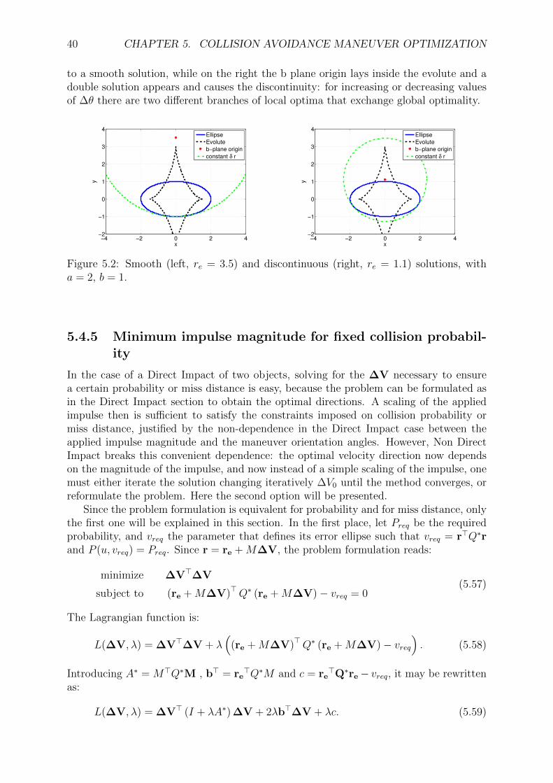
40 CHAPTER 5. COLLISION AVOIDANCE MANEUVER OPTIMIZATION
to a smooth solution, while on the right the b plane origin lays inside the evolute and adouble solution appears and causes the discontinuity: for increasing or decreasing valuesof ∆θ there are two different branches of local optima that exchange global optimality.
−4 −2 0 2 4−2
−1
0
1
2
3
4
x
y
Ellipse
Evolute
b−plane origin
constant δ r
−4 −2 0 2 4−2
−1
0
1
2
3
4
x
y
Ellipse
Evolute
b−plane origin
constant δ r
Figure 5.2: Smooth (left, re = 3.5) and discontinuous (right, re = 1.1) solutions, witha = 2, b = 1.
5.4.5 Minimum impulse magnitude for fixed collision probabil-ity
In the case of a Direct Impact of two objects, solving for the ∆V necessary to ensurea certain probability or miss distance is easy, because the problem can be formulated asin the Direct Impact section to obtain the optimal directions. A scaling of the appliedimpulse then is sufficient to satisfy the constraints imposed on collision probability ormiss distance, justified by the non-dependence in the Direct Impact case between theapplied impulse magnitude and the maneuver orientation angles. However, Non DirectImpact breaks this convenient dependence: the optimal velocity direction now dependson the magnitude of the impulse, and now instead of a simple scaling of the impulse, onemust either iterate the solution changing iteratively ∆V0 until the method converges, orreformulate the problem. Here the second option will be presented.
Since the problem formulation is equivalent for probability and for miss distance, onlythe first one will be explained in this section. In the first place, let Preq be the requiredprobability, and vreq the parameter that defines its error ellipse such that vreq = r>Q∗rand P (u, vreq) = Preq. Since r = re +M∆V, the problem formulation reads:
minimize ∆V>∆V
subject to (re +M∆V)>Q∗ (re +M∆V)− vreq = 0(5.57)
The Lagrangian function is:
L(∆V, λ) = ∆V>∆V + λ(
(re +M∆V)>Q∗ (re +M∆V)− vreq). (5.58)
Introducing A∗ = M>Q∗M , b> = re>Q∗M and c = re
>Q∗re− vreq, it may be rewrittenas:
L(∆V, λ) = ∆V> (I + λA∗) ∆V + 2λb>∆V + λc. (5.59)
5.4. NON-DIRECT IMPACT 41
The minimum value of the Lagrangian function over ∆V is:
∂L
∂∆V= 0⇒∆V = −λ(I + λA∗)†b, (5.60)
where the dagger † means pseudo inverse operation. Using this minimizer of the La-grangian, the dual function is constructed:
g(λ) =
{−λ2b>(I + λA∗)†b + λc, I + λA∗ � 0, b ∈ R(I + λA∗)
−∞ otherwise(5.61)
Using the matrix A∗ eigenvalues λ∗i and eigenvectors s∗i , the problem may be restated as:
maximize g(λ) =−λ2(s∗1>b)2
1 + λ∗1λ+−λ2(s∗2>b)2
1 + λ∗2λ+ λc
subject to − 1
λ∗1≤ λ ≤ 0
(5.62)
which depends only on one variable λ. A necessary condition for optimality comes fromimposing that the previous equation has a null derivative. This condition leads to:
F (λ) =(s∗1>b)2
c
λ(2 + λ∗1λ)
(1 + λ∗1λ)2+
(s∗2>b)2
c
λ(2 + λ∗2λ)
(1 + λ∗2λ)2− 1 = 0. (5.63)
If the non-linear equation above is to be solved using Newton’s Method , it is requiredto provide additional information: the derivative of the function and an initial guess. Thederivative of F with respect to λ is:
dF
dλ=
(s∗1>b)2
c
2
(1 + λ∗1λ)3+
(s∗2>b)2
c
2
(1 + λ∗2λ)3. (5.64)
The initial guess can be estimated as the last time as the maximum value of λ resultingfrom setting s∗i
>b to 0:
λ(0) = max
1
λ∗1
−1 +1√
1− λ∗1c
(s∗1>b)2
,1
λ∗2
−1 +1√
1− λ∗2c
(s∗2>b)2
. (5.65)
When λopt is computed, Eq. (5.61) will provide the optimal impulse ∆Vopt.

42 CHAPTER 5. COLLISION AVOIDANCE MANEUVER OPTIMIZATION
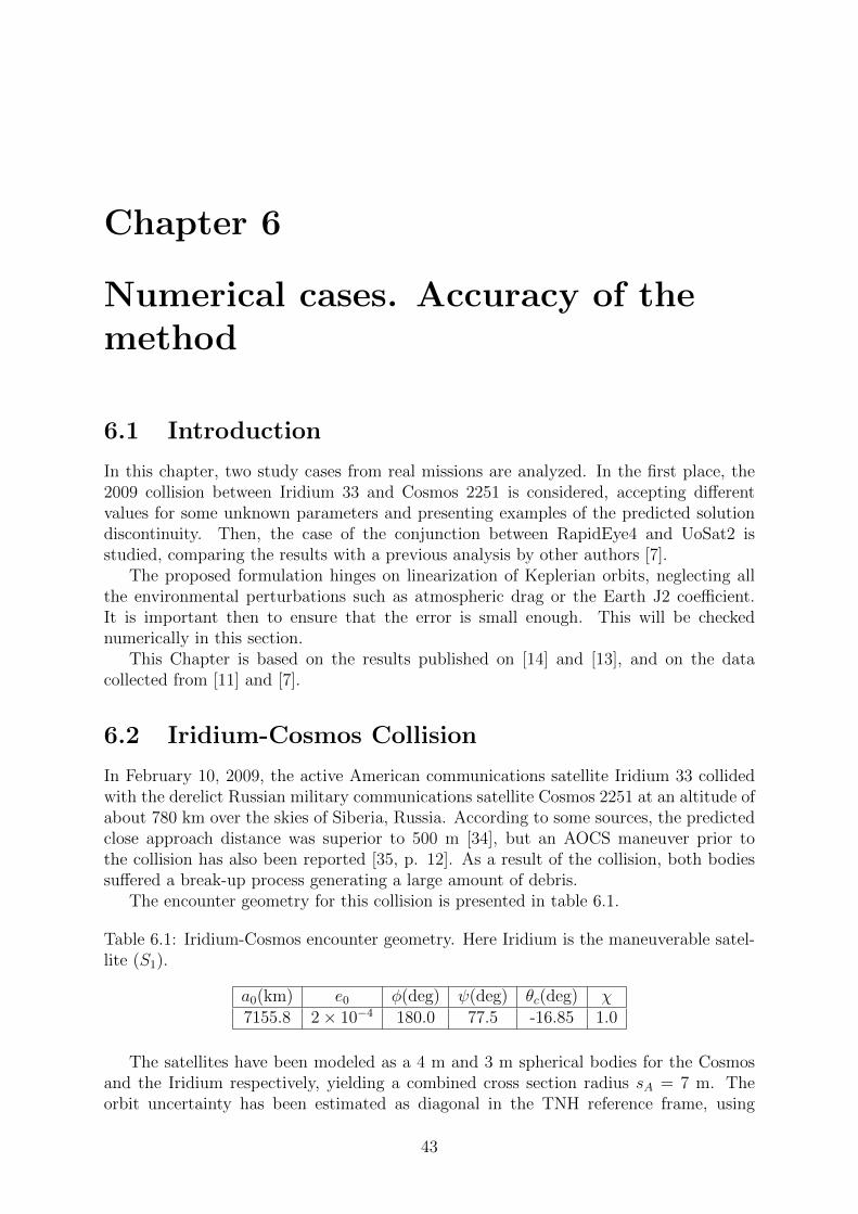
Chapter 6
Numerical cases. Accuracy of themethod
6.1 Introduction
In this chapter, two study cases from real missions are analyzed. In the first place, the2009 collision between Iridium 33 and Cosmos 2251 is considered, accepting differentvalues for some unknown parameters and presenting examples of the predicted solutiondiscontinuity. Then, the case of the conjunction between RapidEye4 and UoSat2 isstudied, comparing the results with a previous analysis by other authors [7].
The proposed formulation hinges on linearization of Keplerian orbits, neglecting allthe environmental perturbations such as atmospheric drag or the Earth J2 coefficient.It is important then to ensure that the error is small enough. This will be checkednumerically in this section.
This Chapter is based on the results published on [14] and [13], and on the datacollected from [11] and [7].
6.2 Iridium-Cosmos Collision
In February 10, 2009, the active American communications satellite Iridium 33 collidedwith the derelict Russian military communications satellite Cosmos 2251 at an altitude ofabout 780 km over the skies of Siberia, Russia. According to some sources, the predictedclose approach distance was superior to 500 m [34], but an AOCS maneuver prior tothe collision has also been reported [35, p. 12]. As a result of the collision, both bodiessuffered a break-up process generating a large amount of debris.
The encounter geometry for this collision is presented in table 6.1.
Table 6.1: Iridium-Cosmos encounter geometry. Here Iridium is the maneuverable satel-lite (S1).
a0(km) e0 φ(deg) ψ(deg) θc(deg) χ7155.8 2× 10⁻⁴ 180.0 77.5 -16.85 1.0
The satellites have been modeled as a 4 m and 3 m spherical bodies for the Cosmosand the Iridium respectively, yielding a combined cross section radius sA = 7 m. Theorbit uncertainty has been estimated as diagonal in the TNH reference frame, using
43
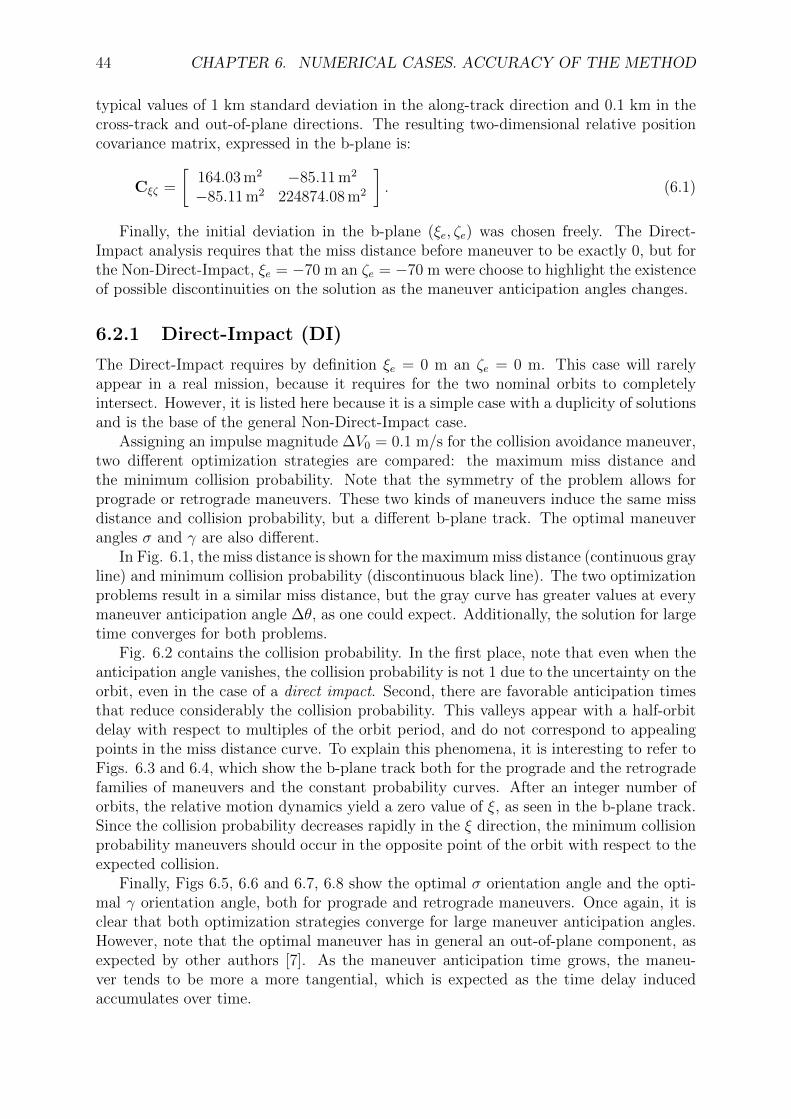
44 CHAPTER 6. NUMERICAL CASES. ACCURACY OF THE METHOD
typical values of 1 km standard deviation in the along-track direction and 0.1 km in thecross-track and out-of-plane directions. The resulting two-dimensional relative positioncovariance matrix, expressed in the b-plane is:
Cξζ =
[164.03 m2 −85.11 m2
−85.11 m2 224874.08 m2
]. (6.1)
Finally, the initial deviation in the b-plane (ξe, ζe) was chosen freely. The Direct-Impact analysis requires that the miss distance before maneuver to be exactly 0, but forthe Non-Direct-Impact, ξe = −70 m an ζe = −70 m were choose to highlight the existenceof possible discontinuities on the solution as the maneuver anticipation angles changes.
6.2.1 Direct-Impact (DI)
The Direct-Impact requires by definition ξe = 0 m an ζe = 0 m. This case will rarelyappear in a real mission, because it requires for the two nominal orbits to completelyintersect. However, it is listed here because it is a simple case with a duplicity of solutionsand is the base of the general Non-Direct-Impact case.
Assigning an impulse magnitude ∆V0 = 0.1 m/s for the collision avoidance maneuver,two different optimization strategies are compared: the maximum miss distance andthe minimum collision probability. Note that the symmetry of the problem allows forprograde or retrograde maneuvers. These two kinds of maneuvers induce the same missdistance and collision probability, but a different b-plane track. The optimal maneuverangles σ and γ are also different.
In Fig. 6.1, the miss distance is shown for the maximum miss distance (continuous grayline) and minimum collision probability (discontinuous black line). The two optimizationproblems result in a similar miss distance, but the gray curve has greater values at everymaneuver anticipation angle ∆θ, as one could expect. Additionally, the solution for largetime converges for both problems.
Fig. 6.2 contains the collision probability. In the first place, note that even when theanticipation angle vanishes, the collision probability is not 1 due to the uncertainty on theorbit, even in the case of a direct impact. Second, there are favorable anticipation timesthat reduce considerably the collision probability. This valleys appear with a half-orbitdelay with respect to multiples of the orbit period, and do not correspond to appealingpoints in the miss distance curve. To explain this phenomena, it is interesting to refer toFigs. 6.3 and 6.4, which show the b-plane track both for the prograde and the retrogradefamilies of maneuvers and the constant probability curves. After an integer number oforbits, the relative motion dynamics yield a zero value of ξ, as seen in the b-plane track.Since the collision probability decreases rapidly in the ξ direction, the minimum collisionprobability maneuvers should occur in the opposite point of the orbit with respect to theexpected collision.
Finally, Figs 6.5, 6.6 and 6.7, 6.8 show the optimal σ orientation angle and the opti-mal γ orientation angle, both for prograde and retrograde maneuvers. Once again, it isclear that both optimization strategies converge for large maneuver anticipation angles.However, note that the optimal maneuver has in general an out-of-plane component, asexpected by other authors [7]. As the maneuver anticipation time grows, the maneu-ver tends to be more a more tangential, which is expected as the time delay inducedaccumulates over time.
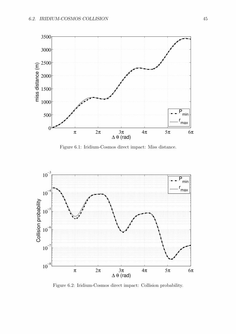
6.2. IRIDIUM-COSMOS COLLISION 45
π 2π 3π 4π 5π 6π0
500
1000
1500
2000
2500
3000
3500
∆ θ (rad)
mis
s d
ista
nce
(m
)
Pmin
rmax
Figure 6.1: Iridium-Cosmos direct impact: Miss distance.
π 2π 3π 4π 5π 6π10
−8
10−7
10−6
10−5
10−4
10−3
∆ θ (rad)
Co
llisio
n p
rob
ab
ility
Pmin
rmax
Figure 6.2: Iridium-Cosmos direct impact: Collision probability.
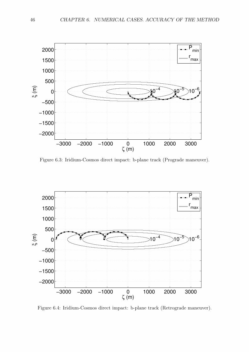
46 CHAPTER 6. NUMERICAL CASES. ACCURACY OF THE METHOD
−3000 −2000 −1000 0 1000 2000 3000
−2000
−1500
−1000
−500
0
500
1000
1500
2000
ζ (m)
ξ (m
)
10−4
10−5
10−6
Pmin
rmax
Figure 6.3: Iridium-Cosmos direct impact: b-plane track (Prograde maneuver).
−3000 −2000 −1000 0 1000 2000 3000
−2000
−1500
−1000
−500
0
500
1000
1500
2000
ζ (m)
ξ (m
)
10−4
10−5
10−6
Pmin
rmax
Figure 6.4: Iridium-Cosmos direct impact: b-plane track (Retrograde maneuver).
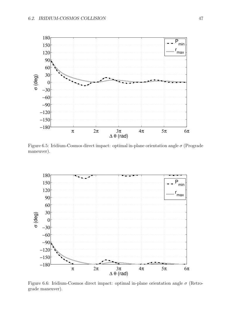
6.2. IRIDIUM-COSMOS COLLISION 47
π 2π 3π 4π 5π 6π−180
−150
−120
−90
−60
−30
0
30
60
90
120
150
180
∆ θ (rad)
σ (
deg
)
Pmin
rmax
Figure 6.5: Iridium-Cosmos direct impact: optimal in-plane orientation angle σ (Progrademaneuver).
π 2π 3π 4π 5π 6π−180
−150
−120
−90
−60
−30
0
30
60
90
120
150
180
∆ θ (rad)
σ (
de
g)
Pmin
rmax
Figure 6.6: Iridium-Cosmos direct impact: optimal in-plane orientation angle σ (Retro-grade maneuver).
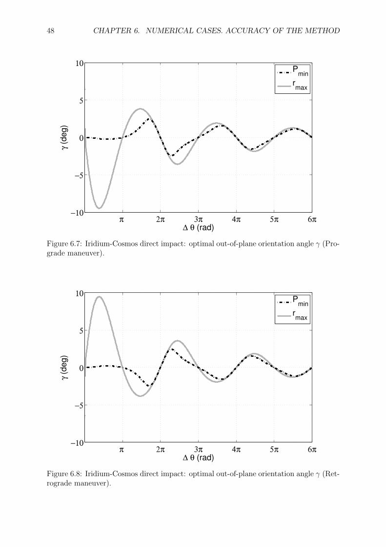
48 CHAPTER 6. NUMERICAL CASES. ACCURACY OF THE METHOD
π 2π 3π 4π 5π 6π−10
−5
0
5
10
∆ θ (rad)
γ (d
eg
)
Pmin
rmax
Figure 6.7: Iridium-Cosmos direct impact: optimal out-of-plane orientation angle γ (Pro-grade maneuver).
π 2π 3π 4π 5π 6π−10
−5
0
5
10
∆ θ (rad)
γ (d
eg
)
Pmin
rmax
Figure 6.8: Iridium-Cosmos direct impact: optimal out-of-plane orientation angle γ (Ret-rograde maneuver).
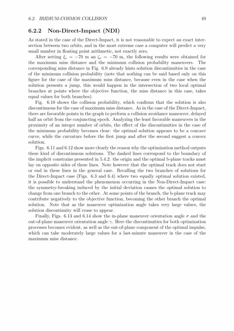
6.2. IRIDIUM-COSMOS COLLISION 49
6.2.2 Non-Direct-Impact (NDI)
As stated in the case of the Direct-Impact, it is not reasonable to expect an exact inter-section between two orbits, and in the most extreme case a computer will predict a verysmall number in floating point arithmetic, not exactly zero.
After setting ξe = −70 m an ζe = −70 m, the following results were obtained forthe maximum miss distance and the minimum collision probability maneuvers. Thecorresponding miss distance in Fig. 6.9 already hints solution discontinuities in the caseof the minimum collision probability (note that nothing can be said based only on thisfigure for the case of the maximum miss distance, because even in the case when thesolution presents a jump, this would happen in the intersection of two local optimalbranches at points where the objective function, the miss distance in this case, takesequal values for both branches).
Fig. 6.10 shows the collision probability, which confirms that the solution is alsodiscontinuous for the case of maximum miss distance. As in the case of the Direct-Impact,there are favorable points in the graph to perform a collision avoidance maneuver, delayedhalf an orbit from the conjuncting epoch. Analyzing the least favorable maneuvers in theproximity of an integer number of orbits, the effect of the discontinuities in the case ofthe minimum probability becomes clear: the optimal solution appears to be a concavecurve, while the curvature before the first jump and after the second suggest a convexsolution.
Figs. 6.11 and 6.12 show more clearly the reason why the optimization method outputsthese kind of discontinuous solutions. The dashed lines correspond to the boundary ofthe implicit constrains presented in 5.4.2: the origin and the optimal b-plane tracks mustlay on opposite sides of these lines. Note however that the optimal track does not startor end in these lines in the general case. Recalling the two branches of solutions forthe Direct-Impact case (Figs. 6.3 and 6.4) where two equally optimal solution existed,it is possible to understand the phenomenon occurring in the Non-Direct-Impact case:the symmetry-breaking induced by the initial deviation causes the optimal solution tochange from one branch to the other. At some points of the branch, the b-plane track maycontribute negatively to the objective function, becoming the other branch the optimalsolution. Note that as the maneuver optimization angle takes very large values, thesolution discontinuity will cease to appear.
Finally, Figs. 6.13 and 6.14 show the in-plane maneuver orientation angle σ and theout-of-plane maneuver orientation angle γ. Here the discontinuities for both optimizationprocesses becomes evident, as well as the out-of-plane component of the optimal impulse,which can take moderately large values for a last-minute maneuver in the case of themaximum miss distance.
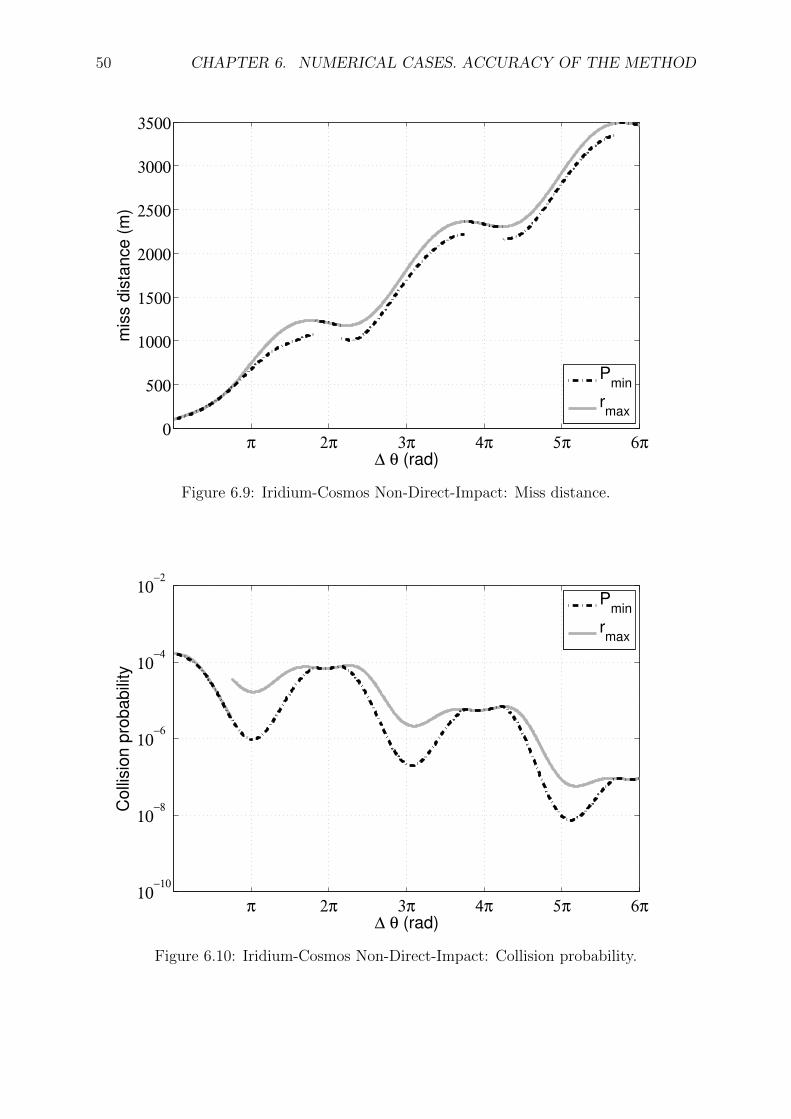
50 CHAPTER 6. NUMERICAL CASES. ACCURACY OF THE METHOD
π 2π 3π 4π 5π 6π0
500
1000
1500
2000
2500
3000
3500
∆ θ (rad)
mis
s d
ista
nce
(m
)
Pmin
rmax
Figure 6.9: Iridium-Cosmos Non-Direct-Impact: Miss distance.
π 2π 3π 4π 5π 6π10
−10
10−8
10−6
10−4
10−2
∆ θ (rad)
Co
llisio
n p
rob
ab
ility
Pmin
rmax
Figure 6.10: Iridium-Cosmos Non-Direct-Impact: Collision probability.
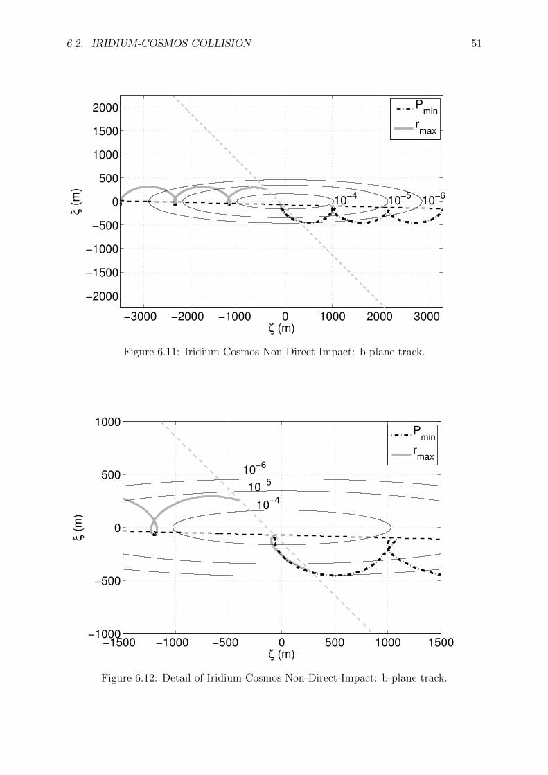
6.2. IRIDIUM-COSMOS COLLISION 51
−3000 −2000 −1000 0 1000 2000 3000
−2000
−1500
−1000
−500
0
500
1000
1500
2000
ζ (m)
ξ (m
)
10−4
10−5
10−6
Pmin
rmax
Figure 6.11: Iridium-Cosmos Non-Direct-Impact: b-plane track.
−1500 −1000 −500 0 500 1000 1500−1000
−500
0
500
1000
ζ (m)
ξ (m
)
10−4
10−5
10−6
Pmin
rmax
Figure 6.12: Detail of Iridium-Cosmos Non-Direct-Impact: b-plane track.
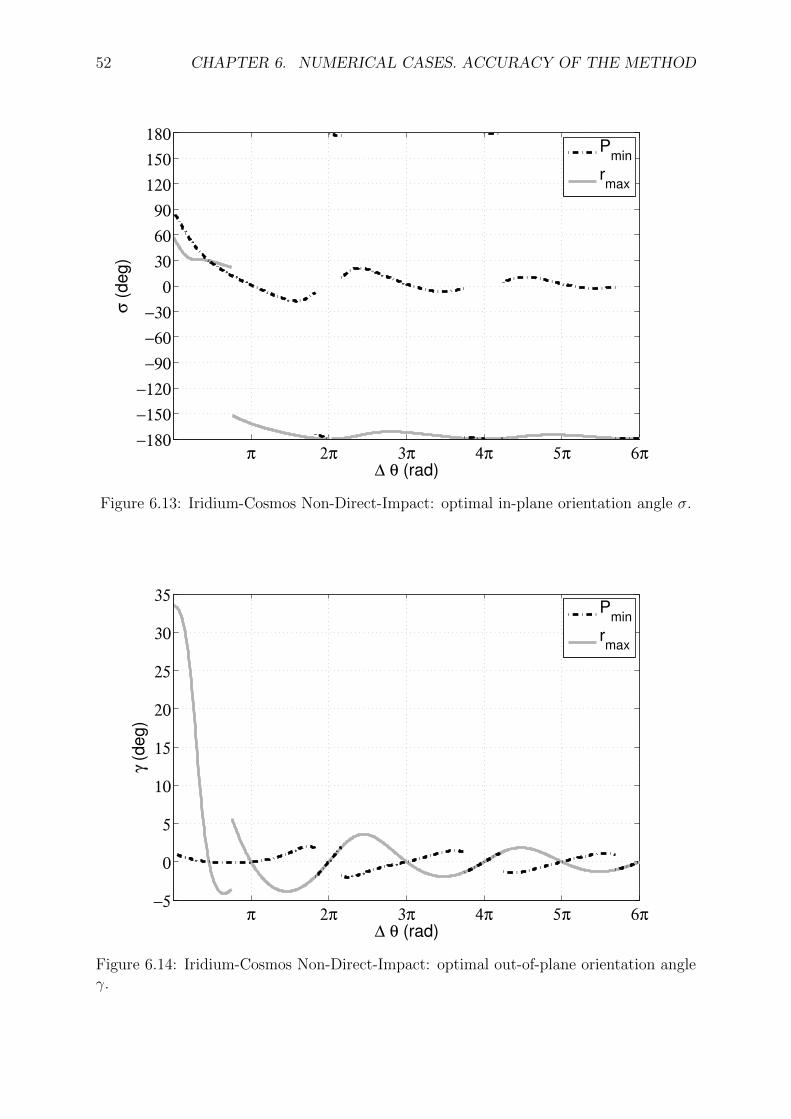
52 CHAPTER 6. NUMERICAL CASES. ACCURACY OF THE METHOD
π 2π 3π 4π 5π 6π−180
−150
−120
−90
−60
−30
0
30
60
90
120
150
180
∆ θ (rad)
σ (
de
g)
Pmin
rmax
Figure 6.13: Iridium-Cosmos Non-Direct-Impact: optimal in-plane orientation angle σ.
π 2π 3π 4π 5π 6π−5
0
5
10
15
20
25
30
35
∆ θ (rad)
γ (d
eg
)
Pmin
rmax
Figure 6.14: Iridium-Cosmos Non-Direct-Impact: optimal out-of-plane orientation angleγ.
6.2. IRIDIUM-COSMOS COLLISION 53
6.2.3 Solution Discontinuity
The solution discontinuity is a novel result that was not pointed out in previous worksby other authors, so it deserves some additional attention. Let us focus on the previousstudied case and analyze in more depth the discontinuity arising for the case of themaximum miss distance at around ∆θ ' 135 deg (see Fig. 6.12, gray curve for example).
As predicted in section 5.4.4, the discontinuities may arise when the semi-major axis ofthe Reachable Domain is parallel to the boundary defined by Eq. (5.53). To illustrate thisresult, Fig. 6.15 contains the b-plane track from ∆θ = 0 to a maximum value in dottedline, constant maximum miss distance contours (this is, circumferences of radius themaximum miss distance for the maximum ∆θ of the figure), and the Elliptical ReachableDomain at the largest ∆θ considered in solid gray. Note that the constant miss distancecircumference and the Elliptical Reachable Domain are tangent at the b-plane intersectionpoint, but up to 4 tangent circumferences are possible: the other points of tangencycorrespond to local optimal maneuvers
Fig. 6.15a shows the b-plane track shortly before the jump, with ∆θ = 100 deg. Sincethere are other non-global optimal solutions corresponding to the four possible tangentcircumferences to the Elliptical Reachable Domain, let us focus on the second largest one,corresponding to the non-global-optimal exterior tangent circumference.
As the maneuver anticipation angle increases, the Elliptical Reachable Domain changessize and orientation, and when ∆θ attains a value close to 135 deg, its semi-major axisbecomes parallel to the boundary of Eq. (5.53), as shown in Fig. 6.15b. At this point,two tangent points appear: one corresponds to the previous global optimal, while theother one emerge from the already mentioned local optimal branch represented by theintersection of the other exterior tangent circumference with the Elliptical ReachableDomain.
This new global-optimal branch can be seen in Fig. 6.15c. Note that the old global-optimal branch as becomes a local optimal solution, and for some time the differencebetween the two remains small.
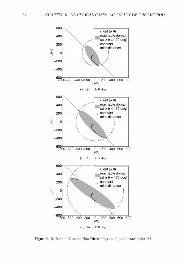
54 CHAPTER 6. NUMERICAL CASES. ACCURACY OF THE METHOD
−800 −600 −400 −200 0 200 400 600 800−600
−400
−200
0
200
400
600
ζ (m)
ξ (m
)
r_opt (∆ θ)
reachable domain
(at ∆ θ = 100 deg)
constantmiss distance
(a) ∆θ = 100 deg.
−800 −600 −400 −200 0 200 400 600 800−600
−400
−200
0
200
400
600
ζ (m)
ξ (m
)
r_opt (∆ θ)
reachable domain
(at ∆ θ = 135 deg)
constantmiss distance
(b) ∆θ = 135 deg.
−800 −600 −400 −200 0 200 400 600 800−600
−400
−200
0
200
400
600
ζ (m)
ξ (m
)
r_opt (∆ θ)
reachable domain
(at ∆ θ = 170 deg)
constantmiss distance
(c) ∆θ = 170 deg.
Figure 6.15: Iridium-Cosmos Non-Direct-Impact: b-plane track after ∆θ.
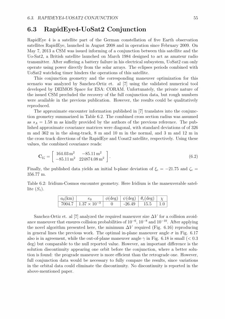
6.3. RAPIDEYE4-UOSAT2 CONJUNCTION 55
6.3 RapidEye4-UoSat2 Conjunction
RapidEye 4 is a satellite part of the German constellation of five Earth observationsatellites RapidEye, launched in August 2008 and in operation since February 2009. OnMay 7, 2013 a CSM was issued informing of a conjunction between this satellite and theUo-Sat2, a British satellite launched on March 1984 designed to act as amateur radiotransmitter. After suffering a battery failure in his electrical subsystem, UoSat2 can onlyoperate using power directly from the solar arrays. The eclipses periods combined withUoSat2 watchdog timer hinders the operations of this satellite.
This conjunction geometry and the corresponding maneuver optimization for thisscenario was analyzed by Sanchez-Ortiz et. al [7] using the validated numerical tooldeveloped by DEIMOS Space for ESA: CORAM. Unfortunately, the private nature ofthe issued CSM precluded the recovery of the full conjunction data, but rough numberswere available in the previous publication. However, the results could be qualitativelyreproduced.
The approximate encounter information published in [7] translates into the conjunc-tion geometry summarized in Table 6.2. The combined cross section radius was assumedas sA = 1.58 m as kindly provided by the authors of the previous reference. The pub-lished approximate covariance matrices were diagonal, with standard deviations of of 326m and 362 m in the along-track, 8 m and 10 m in the normal, and 3 m and 12 m inthe cross track directions of the RapidEye and Uosat2 satellite, respectively. Using thesevalues, the combined covariance reads:
Cξζ =
[164.03 m2 −85.11 m2
−85.11 m2 224874.08 m2
]. (6.2)
Finally, the published data yields an initial b-plane deviation of ξe = −21.75 and ζe =356.77 m.
Table 6.2: Iridium-Cosmos encounter geometry. Here Iridium is the maneuverable satel-lite (S1).
a0(km) e0 φ(deg) ψ(deg) θc(deg) χ7004.7 1.37× 10⁻³ 0 -26.49 15.5 1.0
Sanchez-Ortiz et. al [7] analyzed the required maneuver size ∆V for a collision avoid-ance maneuver that ensures collision probabilities of 10−6, 10−8 and 10−10. After applyingthe novel algorithm presented here, the minimum ∆V required (Fig. 6.16) reproducingin general lines the previous work. The optimal in-plane maneuver angle σ in Fig. 6.17also is in agreement, while the out-of-plane maneuver angle γ in Fig. 6.18 is small (< 0.3deg) but comparable to the null reported value. However, an important difference is thesolution discontinuity appearing one orbit before the conjunction, where a better solu-tion is found: the prograde maneuver is more efficient than the retrograde one. However,full conjunction data would be necessary to fully compare the results, since variationsin the orbital data could eliminate the discontinuity. No discontinuity is reported in theabove-mentioned paper.
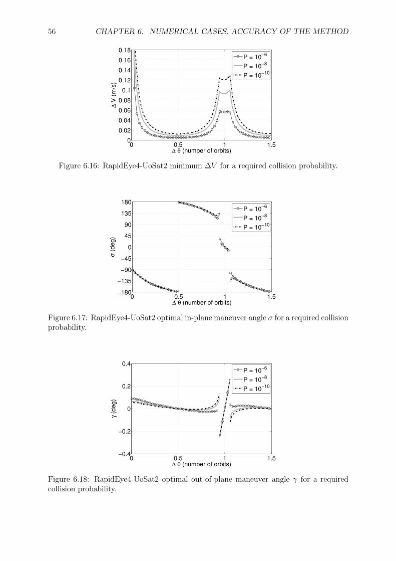
56 CHAPTER 6. NUMERICAL CASES. ACCURACY OF THE METHOD
0 0.5 1 1.50
0.02
0.04
0.06
0.08
0.1
0.12
0.14
0.16
0.18
∆ θ (number of orbits)
∆ V
(m
/s)
P = 10−6
P = 10−8
P = 10−10
Figure 6.16: RapidEye4-UoSat2 minimum ∆V for a required collision probability.
0 0.5 1 1.5−180
−135
−90
−45
0
45
90
135
180
∆ θ (number of orbits)
σ (
de
g)
P = 10−6
P = 10−8
P = 10−10
Figure 6.17: RapidEye4-UoSat2 optimal in-plane maneuver angle σ for a required collisionprobability.
0 0.5 1 1.5−0.4
−0.2
0
0.2
0.4
∆ θ (number of orbits)
γ (d
eg
)
P = 10−6
P = 10−8
P = 10−10
Figure 6.18: RapidEye4-UoSat2 optimal out-of-plane maneuver angle γ for a requiredcollision probability.
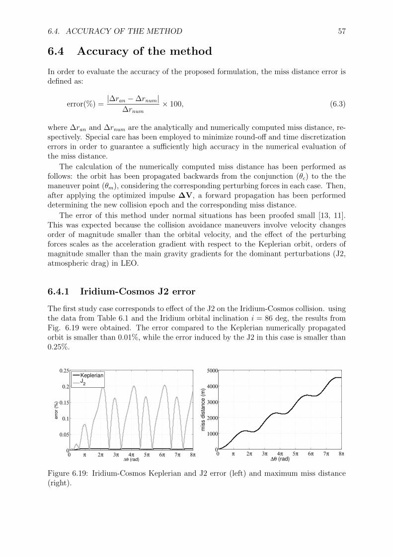
6.4. ACCURACY OF THE METHOD 57
6.4 Accuracy of the method
In order to evaluate the accuracy of the proposed formulation, the miss distance error isdefined as:
error(%) =|∆ran −∆rnum|
∆rnum× 100, (6.3)
where ∆ran and ∆rnum are the analytically and numerically computed miss distance, re-spectively. Special care has been employed to minimize round-off and time discretizationerrors in order to guarantee a sufficiently high accuracy in the numerical evaluation ofthe miss distance.
The calculation of the numerically computed miss distance has been performed asfollows: the orbit has been propagated backwards from the conjunction (θc) to the themaneuver point (θm), considering the corresponding perturbing forces in each case. Then,after applying the optimized impulse ∆V, a forward propagation has been performeddetermining the new collision epoch and the corresponding miss distance.
The error of this method under normal situations has been proofed small [13, 11].This was expected because the collision avoidance maneuvers involve velocity changesorder of magnitude smaller than the orbital velocity, and the effect of the perturbingforces scales as the acceleration gradient with respect to the Keplerian orbit, orders ofmagnitude smaller than the main gravity gradients for the dominant perturbations (J2,atmospheric drag) in LEO.
6.4.1 Iridium-Cosmos J2 error
The first study case corresponds to effect of the J2 on the Iridium-Cosmos collision. usingthe data from Table 6.1 and the Iridium orbital inclination i = 86 deg, the results fromFig. 6.19 were obtained. The error compared to the Keplerian numerically propagatedorbit is smaller than 0.01%, while the error induced by the J2 in this case is smaller than0.25%.
0 π 2π 3π 4π 5π 6π 7π 8π0
0.05
0.1
0.15
0.2
0.25
∆θ (rad)
err
or
(%)
KeplerianJ
2
0 π 2π 3π 4π 5π 6π 7π 8π0
1000
2000
3000
4000
5000
∆θ (rad)
mis
s d
ista
nce
(m
)
Figure 6.19: Iridium-Cosmos Keplerian and J2 error (left) and maximum miss distance(right).
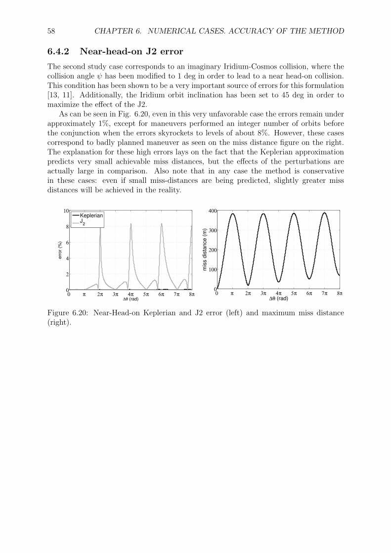
58 CHAPTER 6. NUMERICAL CASES. ACCURACY OF THE METHOD
6.4.2 Near-head-on J2 error
The second study case corresponds to an imaginary Iridium-Cosmos collision, where thecollision angle ψ has been modified to 1 deg in order to lead to a near head-on collision.This condition has been shown to be a very important source of errors for this formulation[13, 11]. Additionally, the Iridium orbit inclination has been set to 45 deg in order tomaximize the effect of the J2.
As can be seen in Fig. 6.20, even in this very unfavorable case the errors remain underapproximately 1%, except for maneuvers performed an integer number of orbits beforethe conjunction when the errors skyrockets to levels of about 8%. However, these casescorrespond to badly planned maneuver as seen on the miss distance figure on the right.The explanation for these high errors lays on the fact that the Keplerian approximationpredicts very small achievable miss distances, but the effects of the perturbations areactually large in comparison. Also note that in any case the method is conservativein these cases: even if small miss-distances are being predicted, slightly greater missdistances will be achieved in the reality.
0 π 2π 3π 4π 5π 6π 7π 8π0
2
4
6
8
10
∆θ (rad)
err
or
(%)
KeplerianJ
2
0 π 2π 3π 4π 5π 6π 7π 8π0
100
200
300
400
∆θ (rad)
mis
s d
ista
nce
(m
)
Figure 6.20: Near-Head-on Keplerian and J2 error (left) and maximum miss distance(right).
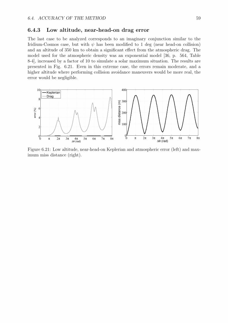
6.4. ACCURACY OF THE METHOD 59
6.4.3 Low altitude, near-head-on drag error
The last case to be analyzed corresponds to an imaginary conjunction similar to theIridium-Cosmos case, but with ψ has been modified to 1 deg (near head-on collision)and an altitude of 350 km to obtain a significant effect from the atmospheric drag. Themodel used for the atmospheric density was an exponential model [36, p. 564, Table8-4], increased by a factor of 10 to simulate a solar maximum situation. The results arepresented in Fig. 6.21. Even in this extreme case, the errors remain moderate, and ahigher altitude where performing collision avoidance maneuvers would be more real, theerror would be negligible.
0 π 2π 3π 4π 5π 6π 7π 8π0
2
4
6
8
10
∆θ (rad)
err
or
(%)
Keplerian
Drag
0 π 2π 3π 4π 5π 6π 7π 8π0
100
200
300
400
∆θ (rad)
mis
s d
ista
nce
(m
)
Figure 6.21: Low altitude, near-head-on Keplerian and atmospheric error (left) and max-imum miss distance (right).

60 CHAPTER 6. NUMERICAL CASES. ACCURACY OF THE METHOD
Chapter 7
OCCAM
7.1 Introduction
The optimization algorithm explained in the present work has been implemented in asoftware tool called OCCAM: Optimal Computation of Collision Avoidance Maneuvers.This software has been registered in the Intellectual Property Register Office of the Comu-nidad de Madrid, with reference number M-004790/2014 and registry number 09-RTPI-05220.7/2014. It is available for Windows and Linux platforms, and uses the MatlabCompiler Runtime (MCR) 2013a libraries. These libraries are included in the distri-bution package of OCCAM, and can additionally be downloaded in the Matlab officialwebpage1.
7.2 How to use
OCCAM user interface main screen is shown in Fig. 7.1. The user must first introducethe scenario data on the left part of the screen, and after pressing calculate a number ofdifferent plots are available on the Results part on the right.
OCCAM takes as input:
• 5 parameters characterizing the collision geometry (the velocity rotation angles ϕand ψ, the velocity scaling ratio χ, and the b-plane offsets ξ0 and ζ0)
• 3 parameters characterizing the shape of the orbit of the maneuverable object (thesemi-major axis a0, the eccentricity e0 and the true anomaly at conjunction epochθc)
• the covariance matrix for the orbits of both objects, expressed in their correspondingUVW reference frame
• the spherical envelope radius for the two objects (rA1, rA2)
Additionally, it is possible to select the optimization criterion to be used: maximummiss distance for fixed fuel consumption, minimum collision probability for fixed fuelconsumption, or minimum fuel consumption for a given required collision probabilitythreshold. The analysis is to be performed a number of orbits before the conjunction,
1 http://www.mathworks.es/products/compiler/mcr/ (accessed September 1, 2014)
61
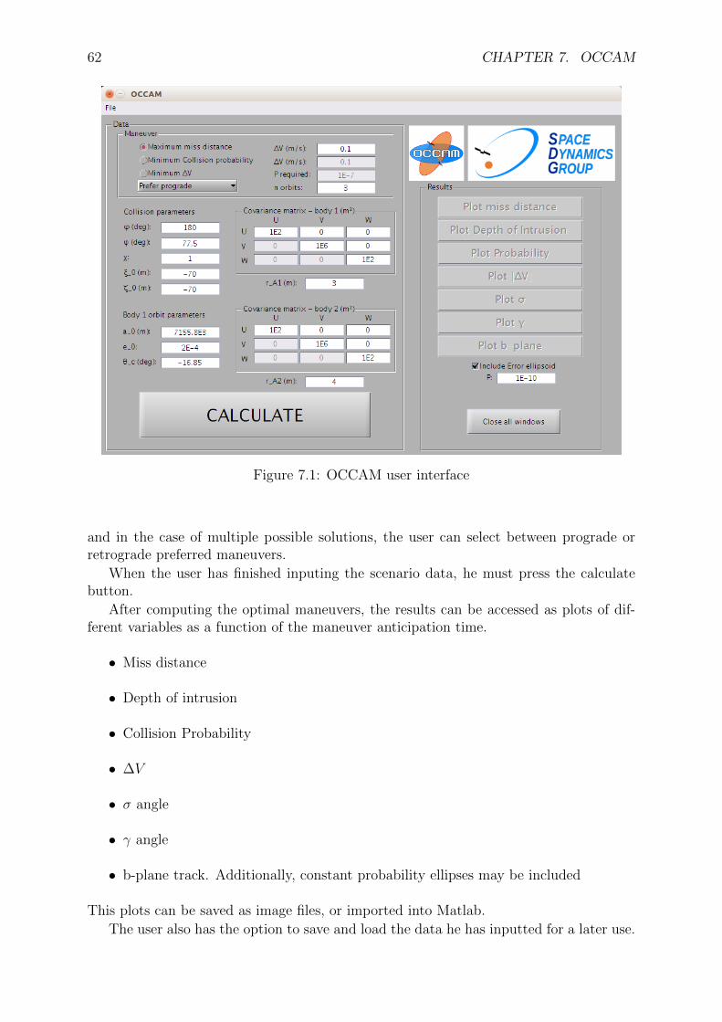
62 CHAPTER 7. OCCAM
Figure 7.1: OCCAM user interface
and in the case of multiple possible solutions, the user can select between prograde orretrograde preferred maneuvers.
When the user has finished inputing the scenario data, he must press the calculatebutton.
After computing the optimal maneuvers, the results can be accessed as plots of dif-ferent variables as a function of the maneuver anticipation time.
• Miss distance
• Depth of intrusion
• Collision Probability
• ∆V
• σ angle
• γ angle
• b-plane track. Additionally, constant probability ellipses may be included
This plots can be saved as image files, or imported into Matlab.
The user also has the option to save and load the data he has inputted for a later use.
7.3. OCCAM COLLISION AVOIDANCE FILES (.ODF) 63
7.3 OCCAM Collision avoidance Files (.odf)
OCCAM has the option to save and load the conjunction scenarios that the user create,so they can be readily available for posterior use. OCCAM uses a simple text file format,storing one variable per line. The relation of variables is presented in table 7.1, andthe default case scenario (Iridium-Cosmos with an arbitrary initial offset) is given as anexample.
7.4 OCCAM lite
In addition to the desktop version of OCCAM, a free demo version is also available on-line2. The on-line version only features the miss distance optimization method for thecase of a Direct Impact, implemented in the JavaScript language. It uses the followinglibraries: jquery3, numeric4 and flot5.
This limited version has two main purposes: the first one is to promote OCCAM andgive to the interested user the possibility to experiment with it before acquiring the mainproduct. The second purpose is to demonstrate how fast is the algorithm presented inthis work: even in a language not designed for scientific computation like JavaScript, themethod is able to calculate the optimal maneuvers up to one orbit before the conjunctionin less than a second.
The interface of OCCAM lite is presented in Fig 7.2, and a comparison of the results ofOCCAM and OCCAM lite for the case of the Iridium-Cosmos direct impact are presentedin Fig. 7.3 and 7.4.
2http://sdg.aero.upm.es/index.php/online-apps/occam-lite (accessed September 1, 2014)3http://jquery.com/ (accessed September 1, 2014)4http://numericjs.com/ (accessed September 1, 2014)5http://www.flotcharts.org/ (accessed September 1, 2014)
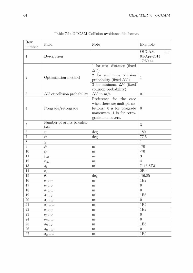
64 CHAPTER 7. OCCAM
Table 7.1: OCCAM Collision avoidance file format
Rownumber
Field Note Example
1 DescriptionOCCAM file04-Apr-201417:50:44
1 for miss distance (fixed∆V )
2 Optimization method2 for minimum collisionprobability (fixed ∆V )
1
3 for minimum ∆V (fixedcollision probability)
3 ∆V or collision probability ∆V in m/s 0.1
4 Prograde/retrograde
Preference for the casewhen there are multiple so-lutions. 0 is for progrademaneuvers, 1 is for retro-grade maneuvers.
0
5Number of orbits to calcu-late
3
6 ϕ deg 1807 ψ deg 77.58 χ 19 ξ0 m -7010 ζ0 m -7011 rA1 m 312 rA2 m 413 a0 m 7115.8E314 e0 2E-415 θc deg -16.8516 σ1,UU m 1E217 σ1,UV m 018 σ1,UW m 019 σ1,V V m 1E620 σ1,V W m 021 σ1,WW m 1E222 σ2,UU m 1E223 σ2,UV m 024 σ2,UW m 025 σ2,V V m 1E626 σ2,V W m 027 σ2,WW m 1E2
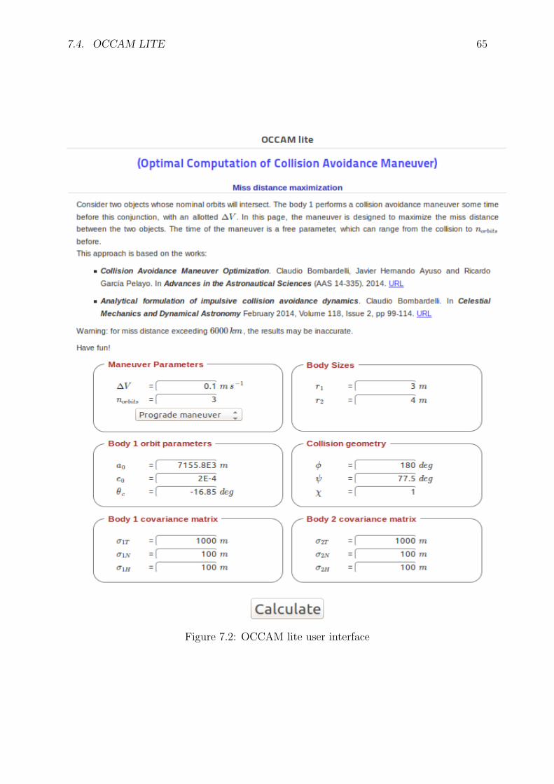
7.4. OCCAM LITE 65
Figure 7.2: OCCAM lite user interface
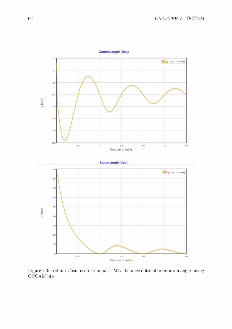
66 CHAPTER 7. OCCAM
Figure 7.3: Iridium-Cosmos direct impact: Miss distance optimal orientation angles usingOCCAM lite
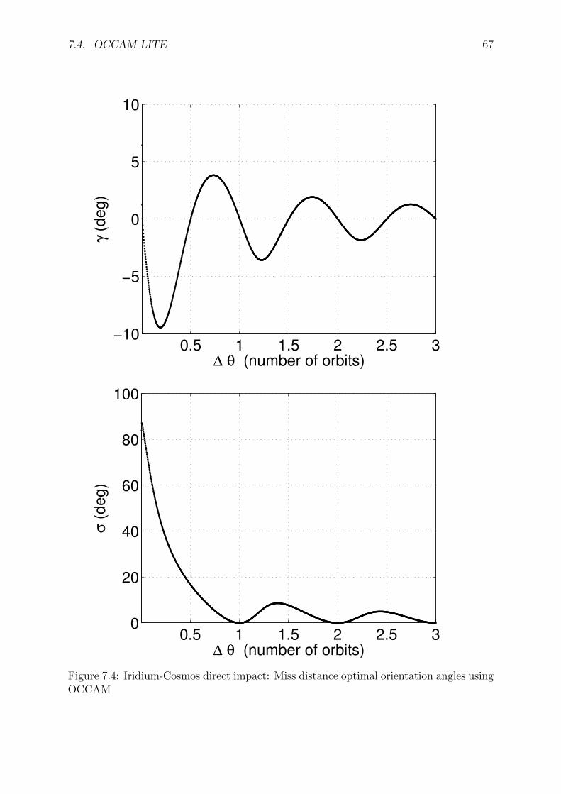
7.4. OCCAM LITE 67
0.5 1 1.5 2 2.5 3−10
−5
0
5
10
∆ θ (number of orbits)
γ (d
eg
)
0.5 1 1.5 2 2.5 30
20
40
60
80
100
∆ θ (number of orbits)
σ (
de
g)
Figure 7.4: Iridium-Cosmos direct impact: Miss distance optimal orientation angles usingOCCAM

68 CHAPTER 7. OCCAM
Chapter 8
Conclusions
8.1 Main contributions of this Thesis work
This work has solved the time-consuming problem of calculating an optimal impulsivecollision avoidance maneuver using a novel fast and accurate approach. The followingresults are highlighted:
The method hinges on the presented linear approximation for the impulsive maneuverdynamics, which has been proved to have high accuracy in the real mission scenarios wherea collision avoidance maneuver would be performed.
Chan’s method for the calculation of the collision probability provides analytical for-mulas that allows fast computations. More importantly, it provides a very good approx-imation for the constant collision probability contours when the combined object radiusis small compared to the uncertainty of the relative motion.
The complex problem of calculating optimal collision avoidance maneuvers has beenreduced to a Quadratically Constrained Quadratic Program (QCQP), a very well studiedoptimization problem. This allows a fast computation of the optimal maneuver, whichrequires solving an eigenvalues and eigenvectors problem coupled with a non-linear equa-tion. This approach is considerably faster than previous methods.
Maximum miss distance collision avoidance maneuvers have been found to be differentfrom the ones that minimize the collision probability in the general case. There exists non-trivial anticipation times before the conjunction that locally optimize the maneuver, withan anticipation time half-period delayed with respect to integer number of orbits of themaneuverable object. The optimal orientation is in general far from tangential and with anon-zero out-of-plane component (note that similar results were obtained by Conway [29]for the asteroid deflection problem). As the maneuver anticipation times tends to infinity,the optimal maneuver tends to a purely tangential (prograde or retrograde) maneuver.
Another novel result reported here is the possible existence of discontinuities in theoptimal maneuver orientation as the maneuver anticipation time varies. This is justifiedby the existence of multiple local optimal branches that exchange global optimality inthe discontinuities.
The accuracy of the method has been found to be high in the practical cases where acollision avoidance maneuver would be performed. The error rises to unacceptable levelsonly in two cases of no practical interest: when performing a maneuver that has littleeffect (i.e. near-head-on collisions) and for very low altitudes orbits where the atmosphericdrag is dominant (note that this objects would re-enter in a brief period of time).
69
70 CHAPTER 8. CONCLUSIONS
8.2 Publications
The present work led to an international conference publication and a JCR (JournalCitation Reports) high impact journal paper:
• C. Bombardelli, J. Hernando-Ayuso, R. Garcıa-Pelayo. Collision Avoidance Ma-neuver Optimization. Advances in the Astronautical Sciences, No. AAS 14-335,Santa Fe, New Mexico, USA, AAS/AIAA, January 26-30 2014.
• C. Bombardelli, J. Hernando-Ayuso. Optimal Impulsive Collision Avoidance in LowEarth Orbit. Journal of Guidance, Control and Dynamics, in Press (accepted onJuly 22, 2014).
8.3 Registered software
The present work also led to the development of OCCAM: Optimal Computation ofCollision Avoidance Maneuvers, a software tool registered in the Intellectual PropertyRegister Office of the Comunidad de Madrid, with reference number M-004790/2014 andregistry number 09-RTPI-05220.7/2014.
Bibliography
[1] Klinkrad, Heiner. Space debris: models and risk analysis. Springer, 2006.
[2] Committee on the Peaceful Uses of Outer Space, various authors. Towards long-term sustainability of space activities: overcoming the challenge of space de-bris. A report of the International interdisciplinary congress on Space debris.a/AC.105/C.1/2011/CRP.14. Available on-line at http://www.oosa.unvienna.org/pdf/limited/AC105_C1_2011_CRP14E.pdf (accessed on September 3 2014).
[3] D. J. Kessler, B. G. Cour-Palais. Collision frequency of artificial satellites: The cre-ation of a debris belt. Journal of Geophysical Research: Space Physics (1978–2012)83.A6 (1978): 2637-2646.
[4] D. J. Kessler; N. L. Johnson, J,-C. Liou, M. Matney The Kessler Syndrome: Impli-cations to Future Space operations. Advances in the Astronautical Sciences, No. AAS10-016, Breckenridge, Colorado, USA, AAS/AIAA, February 6-10 2010.
[5] Conjunction Summary Message Guide. https://www.space-track.org/documents/CSM_Guide.pdf (accessed on June 24, 2014).
[6] J. L. Foster, J. H. Frisbee. Comparison of the Exclusion Volume and ProbabilityThreshold Methods for Debris Avoidance for the STS Orbiter and International SpaceStation. NASA/TP-2007-214571
[7] N. Sanchez-Ortiz, I. Grande-Olalla, J. A. Pulido, K. Merz. Collision Risk Assess-ment and Avoidance Manoeuvres - The new CORAM tool for ESA. 64th InternationalAstronautical Congress, Beijing, China, 2013.
[8] S. Alfano. Collision avoidance maneuver planning tool. 15th AAS/AAIA Astrodynam-ics Specialist Conference, No. AAS 05-308, Lake Tahoe, California, USA, AAS/AIAA,February 6-10 2005.
[9] Jae-Dong Seong, Hae-Dong Kim Collision avoidance maneuvers for multiple threat-ening objects using heuristic algorithms Proceedings of the Institution of MechanicalEngineers, Part G: Journal of Aerospace Engineering 0954410014530678, first pub-lished on April 2, 2014 doi:10.1177/0954410014530678
[10] A. Morselli , R. Armellin, P. Di Lizia ,F. Bernelli-Zazzera Collision Avoidance Ma-neuver Design Based on Multi-objective Optimization . Advances in the AstronauticalSciences, No. AAS 14-148, Santa Fe, New Mexico, USA, AAS/AIAA, January 26-302014.
71
72 BIBLIOGRAPHY
[11] C. Bombardelli. Analytical Formulation of Impulsive Collision Avoidance Dynamics.Celestial Mechanics and Dynamical Astronomy, Vol. 118, No. 2, 2013, pp. 99-114,10.1007/s10569-013-9526-3.
[12] F. Kenneth Chan. Spacecraft Collision Probability. Aerospace Press, 2008.
[13] C. Bombardelli, J. Hernando-Ayuso, R. Garcıa-Pelayo. Collision Avoidance Maneu-ver Optimization. Advances in the Astronautical Sciences, No. AAS 14-335, Santa Fe,New Mexico, USA, AAS/AIAA, January 26-30 2014.
[14] C. Bombardelli, J. Hernando-Ayuso. Optimal Impulsive Collision Avoidance in LowEarth Orbit. Journal of Guidance, Control and Dynamics, in Press (accepted on July22, 2014).
[15] G. B. Valsecchi, A. Milani , G. F. Gronchi , and S. R. Chesley. Resonant returnsto close approaches: Analytical theory. Astronomy and Astrophysics, Vol. 408, No. 3,2003, pp. 1179–1196. DOI: 10.1051/0004-6361:20031039.
[16] SOCRATES: Satellite Orbital Conjunction Reports Assessing Threatening Encoun-ters in Space. http://celestrak.com/SOCRATES/. (accessed on July 15, 2014).
[17] J. Pelaez, J. Hedo, P. de Andres. A special perturbation method in orbital dynamics.Celestial Mechanics and Dynamical Astronomy February 2007, Volume 97, Issue 2,pp 131-150
[18] K. Yamanaka, F. Ankersen. New State Transition Matrix for Relative Motion on anArbitrary Elliptical Orbit . Journal of Guidance, Control, and Dynamics, Vol. 25, No.1 (2002), pp. 60-66.
[19] G. Grimmett, D. Stirzaker. Probability and Random Processes, Second Edition. Ox-ford Science Publications, 1992.
[20] Wiesel, William E. Modern Orbit Determination, Second edition. Aphelion Press,2010.
[21] J. L. Foster and H. S. Estes. A Parametric Analysis of Orbital Debris Collision Prob-ability and Maneuver Rate for Space Vehicles. NASA/JSC-25898. Houston, Texas:NASA Johnson Space Flight Center, August 1992
[22] R. P. Patera. General Method for Calculating Satellite Collision Probability. Jour-nal of Guidance, Control, and Dynamics, Vol. 24, No. 4 (2001), pp. 716-722. doi:10.2514/2.4771
[23] S. Alfano. A Numerical Implementation of Spherical Object Collision Probability.The Journal of the Astronautical Sciences, Vol. 53, No. 1, January-March 2005, pp.103-109
[24] M.R. Akella, K.T. Alfriend. The probability of Collision Between Space Objects. Jour-nal of Guidance, Control, and Dynamics, Vol. 23, No. 5 (2000), pp. 769-772. doi:10.2514/2.4611
[25] S. Alfano Satellite Conjunction Monte Carlo Analysis. Advances in the AstronauticalSciences, No. AAS 09-233, Savannah, Georgia, USA, AAS/AIAA, February 8-12, 2009
BIBLIOGRAPHY 73
[26] S. Alfano Review of Conjunction Probability Method for Short-term Encounters.Advances in the Astronautical Sciences, No. AAS 07-148, Sedona, Arizona, USA,AAS/AIAA, January 28- February 01, 2007
[27] D. Lazaro, P. Righetti. Evolution of EUMETSAT LEO Conjunctions Events Han-dling Operations. The 12th International Conference on Space Operations, No.1287272, 2012. DOI: 10.2514/6.2012-1287272.
[28] V. T. Coppola, J. Woodburn, R. Hujsak. Effects of cross correlated covariance onspacecraft collision probability. Advances in the Astronautical Sciences, No. AAS 04-181, Maui, Hawaii, USA, AAS/AIAA, February 8-12, 2004
[29] B. A. Conway. Near-optimal deflection of Earth-approaching asteroids. Journal ofGuidance , Control and Dynamics, Vol 24, No. 5, 2001, pp. 1035-1037.
[30] S. Boyd and L. Vandenberghe. Convex Optimization. Cambridge University Press,2004.
[31] C. Martel. Advanced Scientific Computations with MATLAB. Notes for the graduatecourse, ETSI Aeronauticos, Technical University of Madrid (UPM), 2014.
[32] C. Wen, Z. Xu, Y. Zhao, Peng Shi Precise Determination of the Reachable Domainfor a Spacecraft with a single impulse .Advances in the Astronautical Sciences, No.AAS 14-371, Santa Fe, New Mexico, USA, AAS/AIAA, January 26-30 2014.
[33] Ellipse Evolute. http://mathworld.wolfram.com/EllipseEvolute.html (accessedon July 23, 2014).
[34] Celestrack: Iridium 33/Cosmos 2251 Collision. http://celestrak.com/events/
collision.asp (accessed on September 8, 2014).
[35] N. Berend. Improvement of collision risk indicators. P2ROTECT FP-7-Space-26820.First P2ROTECT Workshop, Tubitak Uzay, Ankara, 20 March 2012.
[36] D. A. Vallado. Fundamentals of Astrodynamics and Applications , 3rd editionSpringer Science & Business Media 2007.