MeccanicaDOI 10.1007/s11012-010-9283-2

S I M U L AT I O N , O P T I M I Z AT I O N & I D E N T I F I C AT I O N

A new method to approximate the field of movementsof 1-DOF linkages with lower-pairs

Alvaro Noriega · Jose Luis Cortizo ·Eduardo Rodriguez · Ricardo Vijande ·Jose Manuel Sierra

Received: 5 February 2009 / Accepted: 21 January 2010© Springer Science+Business Media B.V. 2010

Abstract This paper presents a new method to ob-tain an approximation of the field of movements of1-DOF linkages with lower pairs. The method is basedon a linkage representation by natural coordinates andthe storage of the constraint equations by means of asparse cubic matrix. To obtain a discrete approxima-tion of the field of movements, a three-stage process isused. In the first stage, a special Evolution Strategy isapplied to make the population converges towards thezones where the constraints’ error is minimal, obtain-ing, at the same time, a good distribution of individu-als. In the second stage, the final individuals of the ESare used as initial points for an optimization algorithmto obtain a greater accuracy. Later, the third stage is afiltering process to eliminate individuals that representnon-desired solutions. This method has been tested onsome linkages with well-known fields of movements,generating comprehensive outcomes that justify thevalidity of the method.

Keywords Linkage · Position problem ·Optimization · Evolution strategy

A. Noriega (�) · J.L. Cortizo · E. Rodriguez · R. Vijande ·J.M. SierraUniversity of Oviedo, Campus Universitario, Edf. Oeste,Módulo 5 s/n, 33203 Gijón, Spaine-mail: noriegaalvaro@uniovi.es

1 Introduction

The direct position problem of a linkage consists ofcalculating the position of all its elements when thevalue of the degrees of freedom (DOFs) is known [9].Two approaches to pose this problem exist. The geo-metric approach, which is the most used, is based onconsidering every element of the linkage as an in-dependent solid, obtaining its position in the spacefrom the solution of the equations which are im-posed by the geometric constraints [9]. The energy-approach is based on the finite elements and it appliesfinite elements techniques to solve the kinematic prob-lems [3, 4]. This approach is not discussed in this pa-per.

In the case of the geometric approach, the equationsthat define the linkage are nonlinear. As a result, the di-rect position problem usually has several possible so-lutions and even, in some cases, it has no solution.

To solve the nonlinear system of equations whichthe geometric approach to the position problem gener-ates, different methods can be used. Newton’s methodis a direct method which has quadratic convergence inthe neighborhood of each root and is easy to imple-ment. This method needs the Jacobian matrix of thesystem to be known. In this method, it is very impor-tant to have a good starting point since the success ofthe algorithm depends on this [13]. Other approachesare indirect since they turn the problem of obtainingthe roots of the system into a minimization problem ofan error function that measures the non-fulfillment of

Meccanica

the system’s equations. Therefore, different optimiza-tion methods can be used. These methods can be clas-sified according to the order of the derivatives that theyuse. Then, we can distinguish between the first ordermethods, which use the gradient’s information of thefunction error and the second order methods, whichalso use the information of the Hessian matrix. Allthese methods always need a starting point and theyprovide only one of the multiple solutions that are pos-sible for the direct position problem.

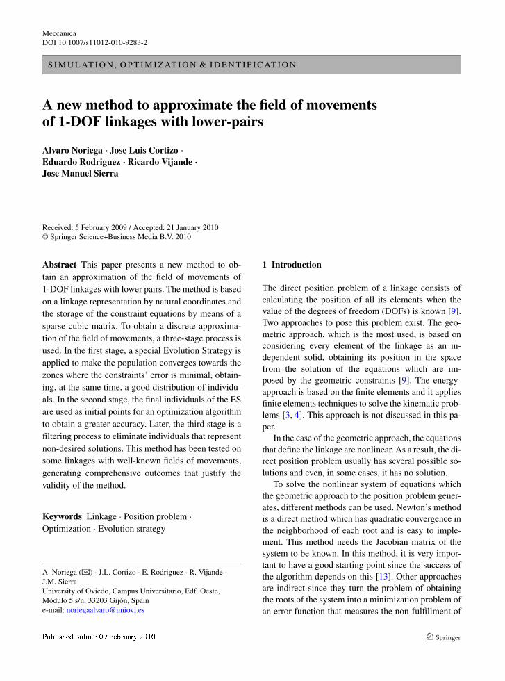
The possible solutions that the position of a linkagecan have can come from two situations. The first situ-ation is to place an element of the linkage in a differ-ent position without affecting the rest of the linkage.An example of this is the triangular element 2-3-5 inthe four-bar linkage of the Fig. 1a which can also beplaced in position 2-3-5′. The other possible situationis the existence of more than one possibility of assem-bly of the linkage as is shown in Fig. 1b.

The multiplicity of solutions shown in Fig. 1b gen-erates different branches of operation in the linkage.These branches can cut each other causing singularconfigurations that complicate the linkage simulation.A classification of the types of singular configurationscan be seen in [23] and [2]. In the singular configura-tions, some branches converge into one creating a mul-tiple root of the system of equations. At these points,the Jacobian matrix of the equations’s system is ill-conditioned and a method like the Newton one wouldlose accuracy. Moreover, there is the possibility that

Fig. 1 Multiplicity of solutions in direct position problem

a non-desired branch of movement is selected to con-tinue the finite displacements problem.

For this reason, a method to obtain an approxima-tion of the complete field of movements of a linkagewithout deforming its elements would be desirable.Furthermore, the method would be immune to the ex-istence of singular configurations in this field.

The paper is organized as follows: In Sect. 2,the modelization by means of natural coordinates oflower-pair linkages and its representation by meanscubic matrix are shown. In Sect. 3, the method to ob-tain a discrete approximation of the field of move-ments of a linkage is shown. In Sect. 4, some examplesof the use of the method are shown. Finally, some con-clusions about the new representation of linkages andthe method proposed to obtain its field of movementsare shown in Sect. 5.

2 Modelization and representation of linkages

The definition of a linkage can be made by a set of co-ordinates which will be the parameters that completelydefine the position of all its elements. Consequently,the variation of these parameters regarding the timedescribes the movement of the linkage [9].

The choice of these coordinates has great impor-tance since it sets the modelization rules, the numberand the complexity of the equations and other factors.

There exist different methods to modelize linkages.Some methods are based on finite elements [3, 4] andthey show the advantage of a simple representation ofthe linkage by means of a geometric matrix. This ma-trix is derived from the stiffness matrix of the linkageif it were modelized as a truss and it condenses all thegeometric information about the linkage.

Moreover, there exist the modelizations mentionedin [9] where the independent and dependent coordi-nates are described. The independent coordinates rep-resent a classic approach for the linkages analysiswhile the dependent coordinates generate a system ofnonlinear constraint equations that is better adapted tonumerical computation. At the same time, the depen-dent coordinates can be classified as relative coordi-nates, reference point coordinates and natural coordi-nates.

The natural coordinates or fully Cartesian are anevolution of the reference point coordinates [8] wherethe reference points are moved to the pairs to avoid

Meccanica

Fig. 2 Examples of constraint equations in 2D

the use of angular variables to define the elements’orientation. They have been selected to this researchbecause they have a simple and systematic definitionof the constraint equations and a smaller number ofcoordinates and equations than the reference point co-ordinates.

2.1 Basic points and constraint equations

The modelization in natural coordinates has two basicsteps. The first step is the definition of the linkage’selements by means of basic points and the second stepis the construction of the constraint equations.

The basic points are situated in accordance withrules specified in [9] and their Cartesian coordinateswill completely define the linkage position. To definea linkage in this particular application, the Cartesiancoordinates of the basic points will be exclusively usedavoiding the use of angles. This eliminates the use ofmixed coordinates because they generate trigonomet-ric nonlinearities in the constraint equations and, aswill be shown later, it is incompatible with the ap-proach by means of cubic matrix representation.

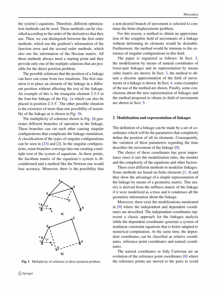
The construction of the constraint equations ismade in accordance with rules specified in [9] and canbe extended both to planar linkage and to spatial ones.In Fig. 2, three examples of constraints equations in aplanar linkage are shown.

The posed constraint equations exclusively de-scribe the linkage’s geometry with lower pairs andthey depend on a set of coordinates (stored in a vec-tor x) where the DOFs are included. Then, the sys-tem of constraint equations has more unknowns than

equations and it is undetermined. In exchange, the so-lutions of this system are all the undeformed possiblepositions of the linkage, it means, the complete fieldof movements of the linkage.

It is worth noting that all the constraint equationsin Fig. 2 are nonlinear but they have a common struc-ture. They are quadratic and are composed with sec-ond order terms in which a constant multiplies a prod-uct of two variables and there can also exist indepen-dent terms. If trigonometric terms were included, therewould not be a common and simple structure.

2.2 Cubic matrix representation

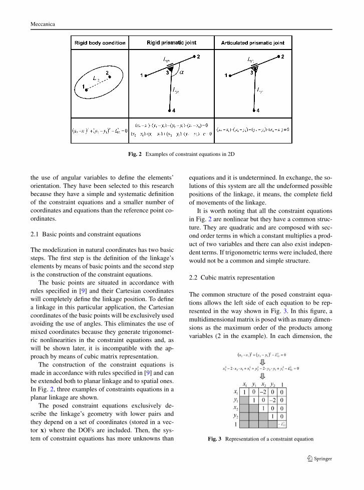
The common structure of the posed constraint equa-tions allows the left side of each equation to be rep-resented in the way shown in Fig. 3. In this figure, amultidimensional matrix is posed with as many dimen-sions as the maximum order of the products amongvariables (2 in the example). In each dimension, the

Fig. 3 Representation of a constraint equation

Meccanica

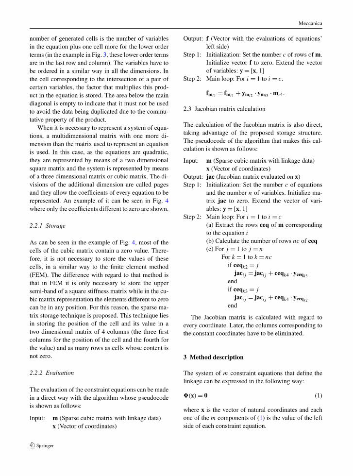
number of generated cells is the number of variablesin the equation plus one cell more for the lower orderterms (in the example in Fig. 3, these lower order termsare in the last row and column). The variables have tobe ordered in a similar way in all the dimensions. Inthe cell corresponding to the intersection of a pair ofcertain variables, the factor that multiplies this prod-uct in the equation is stored. The area below the maindiagonal is empty to indicate that it must not be usedto avoid the data being duplicated due to the commu-tative property of the product.

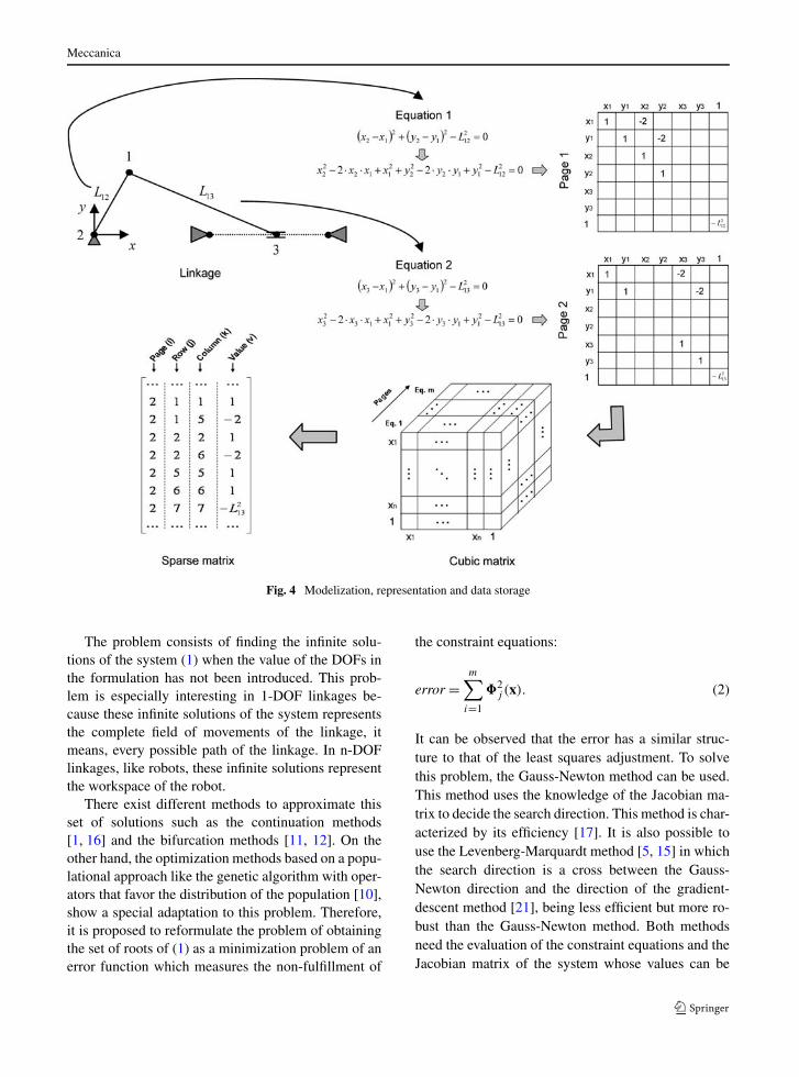
When it is necessary to represent a system of equa-tions, a multidimensional matrix with one more di-mension than the matrix used to represent an equationis used. In this case, as the equations are quadratic,they are represented by means of a two dimensionalsquare matrix and the system is represented by meansof a three dimensional matrix or cubic matrix. The di-visions of the additional dimension are called pagesand they allow the coefficients of every equation to berepresented. An example of it can be seen in Fig. 4where only the coefficients different to zero are shown.

2.2.1 Storage

As can be seen in the example of Fig. 4, most of thecells of the cubic matrix contain a zero value. There-fore, it is not necessary to store the values of thesecells, in a similar way to the finite element method(FEM). The difference with regard to that method isthat in FEM it is only necessary to store the uppersemi-band of a square stiffness matrix while in the cu-bic matrix representation the elements different to zerocan be in any position. For this reason, the sparse ma-trix storage technique is proposed. This technique liesin storing the position of the cell and its value in atwo dimensional matrix of 4 columns (the three firstcolumns for the position of the cell and the fourth forthe value) and as many rows as cells whose content isnot zero.

2.2.2 Evaluation

The evaluation of the constraint equations can be madein a direct way with the algorithm whose pseudocodeis shown as follows:

Input: m (Sparse cubic matrix with linkage data)x (Vector of coordinates)

Output: f (Vector with the evaluations of equations’left side)

Step 1: Initialization: Set the number c of rows of m.Initialize vector f to zero. Extend the vectorof variables: y = [x,1]

Step 2: Main loop: For i = 1 to i = c.

fmi1 = fmi1 + ymi2 · ymi3 · mi4.

2.3 Jacobian matrix calculation

The calculation of the Jacobian matrix is also direct,taking advantage of the proposed storage structure.The pseudocode of the algorithm that makes this cal-culation is shown as follows:

Input: m (Sparse cubic matrix with linkage data)x (Vector of coordinates)

Output: jac (Jacobian matrix evaluated on x)

Step 1: Initialization: Set the number c of equationsand the number n of variables. Initialize ma-trix jac to zero. Extend the vector of vari-ables: y = [x,1]

Step 2: Main loop: For i = 1 to i = c

(a) Extract the rows ceq of m correspondingto the equation i

(b) Calculate the number of rows nc of ceq(c) For j = 1 to j = n

For k = 1 to k = nc

if ceqk2 = j

jacij = jacij + ceqk4 · yceqk3

endif ceqk3 = j

jacij = jacij + ceqk4 · yceqk2

end

The Jacobian matrix is calculated with regard toevery coordinate. Later, the columns corresponding tothe constant coordinates have to be eliminated.

3 Method description

The system of m constraint equations that define thelinkage can be expressed in the following way:

�(x) = 0 (1)

where x is the vector of natural coordinates and eachone of the m components of (1) is the value of the leftside of each constraint equation.

Meccanica

Fig. 4 Modelization, representation and data storage

The problem consists of finding the infinite solu-tions of the system (1) when the value of the DOFs inthe formulation has not been introduced. This prob-lem is especially interesting in 1-DOF linkages be-cause these infinite solutions of the system representsthe complete field of movements of the linkage, itmeans, every possible path of the linkage. In n-DOFlinkages, like robots, these infinite solutions representthe workspace of the robot.

There exist different methods to approximate thisset of solutions such as the continuation methods[1, 16] and the bifurcation methods [11, 12]. On theother hand, the optimization methods based on a popu-lational approach like the genetic algorithm with oper-ators that favor the distribution of the population [10],show a special adaptation to this problem. Therefore,it is proposed to reformulate the problem of obtainingthe set of roots of (1) as a minimization problem of anerror function which measures the non-fulfillment of

the constraint equations:

error =m∑

i=1

�2j (x). (2)

It can be observed that the error has a similar struc-ture to that of the least squares adjustment. To solvethis problem, the Gauss-Newton method can be used.This method uses the knowledge of the Jacobian ma-trix to decide the search direction. This method is char-acterized by its efficiency [17]. It is also possible touse the Levenberg-Marquardt method [5, 15] in whichthe search direction is a cross between the Gauss-Newton direction and the direction of the gradient-descent method [21], being less efficient but more ro-bust than the Gauss-Newton method. Both methodsneed the evaluation of the constraint equations and theJacobian matrix of the system whose values can be

Meccanica

easily computed with the representation indicated inSect. 2.

The fact that there exist infinite solutions to theproblem makes it has a great similarity with the prob-lem of getting the Pareto optimal front by means ofmultiobjective evolutive algorithms [14]. These algo-rithms try to approximate this front by means of fi-nite population P of solutions x (called individuals).The difference is that, in this case, the decision spacehas only one dimension (the error of each solution try-ing to fulfill the constraint equations) and the homoge-neous distribution of solutions must be obtained in thesearch space. This means that the posed problem doesnot fit any of the existent types of multiobjective prob-lems since in this case the final aim is the populationin the search space and not in the decision space.

Then, the proposed method tries to approximate allthe existing branches of movement of a 1-DOF link-age in a simultaneous process by means of a popula-tion of individuals that are distributed the most homo-geneously possible. Branch of movement refers to onethe two possible situations indicated in Fig. 1b.

The method has three sequential stages:

1. Approximation

Its aim is to get a population as well-distributedas possible and where the individuals have the small-est possible error using a special Evolution Strategy(ES).

2. Refinement

Its aim is to reduce to the minimum the error ofthe population’s individuals obtained in the first stageby means of the Levenberg-Marquardt least squaresmethod.

3. Filtering

Its aim is to eliminate, by means of a filteringprocess, the individuals of the population which be-long to branches of operation that produce non-desiredconfigurations in some elements of the linkage or thatrepresent linkages that are impossible to carry out inreal applications.

3.1 Stage 1: Approximation

In this stage, an Evolution Strategy [20] of type(μ,μ)-ES is used. This ES is based on the Discrete Di-rections Mutation Evolution Strategy (DDM-ES) [19]and on the Hybrid Evolution Strategy (H-ES) [18].

This ES exclusively uses the mutation operatorwhich is applied to every individual of the population(called parent), generating an offspring to replace it-self, according to the following expression:

xoffspring = xparent + v · d (3)

where v is the mutation step that is randomly gener-ated according to a Gaussian distribution of mean 0and standard deviation σ (called mutation strength).

To decide the direction of the mutation of each in-dividual (d), an additional knowledge about the objec-tive function is used since the gradient vector of theerror function has the following expression:

∇error =[

∂error

∂x1· · · ∂error

∂xn

](4)

being

∂error

∂xj

= ∂

∂xj

∑

i

�2i (x)

= 2 ·∑

i

�i (x) · ∂�i(x)

∂xj

. (5)

The construction of the gradient vector depends ex-clusively on values of the evaluations of the equationsand on the derivatives contained in the Jacobian ma-trix. These values are easily calculated by means ofthe sparse cubic matrix representation of the constraintequations shown in Sect. 2.

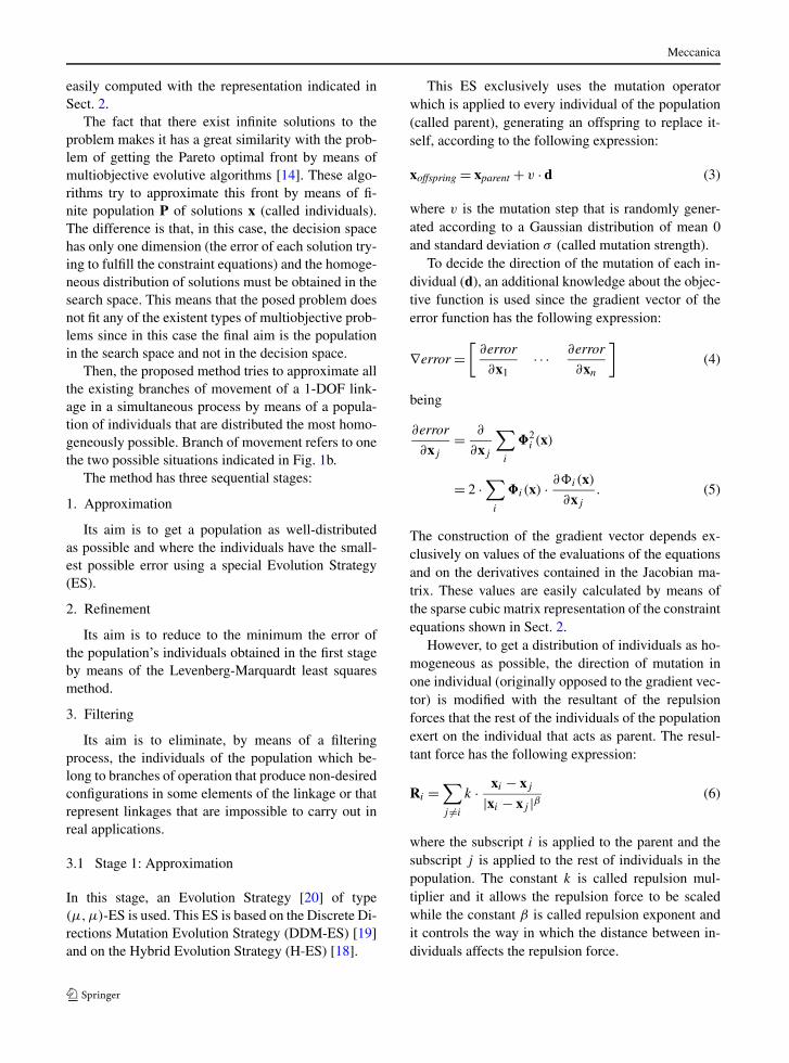
However, to get a distribution of individuals as ho-mogeneous as possible, the direction of mutation inone individual (originally opposed to the gradient vec-tor) is modified with the resultant of the repulsionforces that the rest of the individuals of the populationexert on the individual that acts as parent. The resul-tant force has the following expression:

Ri =∑

j �=i

k · xi − xj

|xi − xj |β (6)

where the subscript i is applied to the parent and thesubscript j is applied to the rest of individuals in thepopulation. The constant k is called repulsion mul-tiplier and it allows the repulsion force to be scaledwhile the constant β is called repulsion exponent andit controls the way in which the distance between in-dividuals affects the repulsion force.

Meccanica

Fig. 5 Graphical example of repulsion forces and direction ofmutation in 2 dimensions

The unit vector that indicates the corrected muta-tion direction is constructed as follows:

di = −∇errori + Ri

| − ∇errori + Ri | . (7)

An example of the process described above can beseen in Fig. 5.

Due to the fact that every variable in the searchspace cannot have the same range of variation, it isproposed to normalize all the ranges to the range [0,1]forming an auxiliary space called workspace whereevolution process happens. When the individuals needto be evaluated, a scaling process has to be done tocarry them to the search space. The expression for thisprocess is the following:

xk = lk + (uk − lk) · x′k (8)

where x is the vector that represents the individual inthe search space, x′ is the vector that represents the in-dividual in the workspace, l is the vector that containsthe lower bound of the variables and u is the vectorwith the upper bound of the variables. Moreover, asthe unit vector d refers to the search space, it must bealso normalized to the workspace in order to use it inthe mutation.

The normalization of the individuals to the work-space is also used to set a single common mutationstrength σ . This mutation strength has a dynamic con-trol which decreases the value of σ with the number of

generations according to the next expression:

σ = s · c1 + (σini − s) (9)

being

s = σend − σini

g − 1(10)

where c1 is the number of the current generation, g

is the number of total generations to make, σini is themutation strength to apply in the initial generation andσend is the mutation strength to apply in the final gen-eration. The mutation strength diminishes in a linearway with the generations.

The selection operator has no sense in this ES be-cause it is desired that the whole population convergestowards the solution, covering it with a homogeneousdistribution. It does that this ES really works as μ evo-lution strategies of type (1,1)-ES together.

There also exists an auxiliary operator which gen-erates independent individuals to complete the popu-lation if the offspring is situated out of the workspace(repair operator). These independent individuals arerandomly generated by the repair operator accordingto a uniform distribution in the workspace.

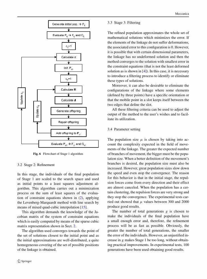
The flowchart of this Stage can be seen in Fig. 6and the following explanations must be given:

• The initial population is randomly generated ac-cording to a uniform distribution in the workspace.The population size μ is defined by the user.

• The evaluation of the population entails the previ-ous scaling process of the individuals to the searchspace and it includes the calculation of the errormade on the fulfillment of the constraint equationsand the calculation of its gradient.

• c1 counts the number of generations executed by thealgorithm. The total number of generations g is pre-viously defined by the user.

• The final mutation strength σend , the repulsion mul-tiplier k and the repulsion exponent β are definedby the user.

• c2 counts the number of individuals of the popula-tion on which the offspring, which replaces its par-ent, has already been generated.

• The repair operator acts when the offspring gener-ated by mutation does not belong to the workspaceand it replaces the parent with an independent indi-vidual.

Meccanica

Fig. 6 Flowchart of Stage 1 algorithm

3.2 Stage 2: Refinement

In this stage, the individuals of the final populationof Stage 1 are scaled to the search space and usedas initial points to a least squares adjustment al-gorithm. This algorithm carries out a minimizationprocess on the sum of least squares of the evalua-tion of constraint equations shown in (2), applyingthe Levenberg-Marquardt method with line search bymeans of mixed quad-cubic interpolation [15].

This algorithm demands the knowledge of the Ja-cobian matrix of the system of constraint equationswhich is easily computed by means of the sparse cubicmatrix representation shown in Sect. 2.

The algorithm used converges towards the point ofthe set of solutions closest to the initial point and asthe initial approximations are well-distributed, a quitehomogeneous covering of the set of possible positionsof the linkage is obtained.

3.3 Stage 3: Filtering

The refined population approximates the whole set ofmathematical solutions which minimizes the error. Ifthe elements of the linkage do not suffer deformations,the associated error to this configuration is 0. However,it is possible that with certain dimensional parameters,the linkage has no undeformed solution and then themethod converges to the solution with smallest error inthe constraint equations (that is not the least deformedsolution as is shown in [4]). In this case, it is necessaryto introduce a filtering process to identify or eliminatethese types of solutions.

Moreover, it can also be desirable to eliminate theconfigurations of the linkage where some elements(defined by three points) have a specific orientation orthat the mobile point in a slot keeps itself between thetwo edges that define the slot.

All these filtering criteria can be used to adjust theoutput of the method to the user’s wishes and to facil-itate its utilization.

3.4 Parameter setting

The population size μ is chosen by taking into ac-count the complexity expected in the field of move-ments of the linkage. The greater the expected numberof branches of movement, the bigger must be the popu-lation size. When a better definition of the movement’sbranches is desired, the population size must also beincreased. However, great population sizes slow downthe speed and even stop the convergence. The reasonfor this behavior is that in the initial stage, the repul-sion forces come from every direction and their effectare almost canceled. When the population has a cer-tain clustering, the repulsion forces are very strong andthey stop the convergence. The experimental tests car-ried out showed that μ values between 300 and 2000produce good results.

The number of total generations g is chosen tomake the individuals of the final population havea small enough error and, therefore, the refinementprocess will be as fast as possible. Obviously, thegreater the number of total generations, the smallerthe error of the individuals. However, an unjustified in-crease in g makes Stage 1 be too long, without obtain-ing practical improvements. In experimental tests, 100generations have been used obtaining good results.

Meccanica

The mutation strength for the initial generation σini

is calculated with the following expression:

σini =√

n

2·(

1

μ

) 1n

(11)

where n is the number of variables. This expression issimilar to the one used in DDM-ES [19]. The choiceof the mutation strength for the final generation σend

depends on the accuracy desired. The value of σend

must be smaller than σini. However, a very small valueof σend can slow down the convergence of the ES inthe first Stage. In the tests carried out, and with 100generations, a value of σend approximately 100 timessmaller than σini generates good results.

The value of the repulsion multiplier k depends onthe population size. If there is a big population size, asmall value of k must be chosen to avoid the repulsionhindering the algorithm convergence and vice versa. Inthe tests carried out, values between 1 and 0.01 wereused depending on the problem. For the repulsion ex-ponent β , the value 1 is usually chosen although insome cases it is observed that with a value of 2, betterresults are obtained but it depends on the number ofvariables and on their ranges in the search space sinceboth values define the magnitude of the distance be-tween individuals.

4 Examples

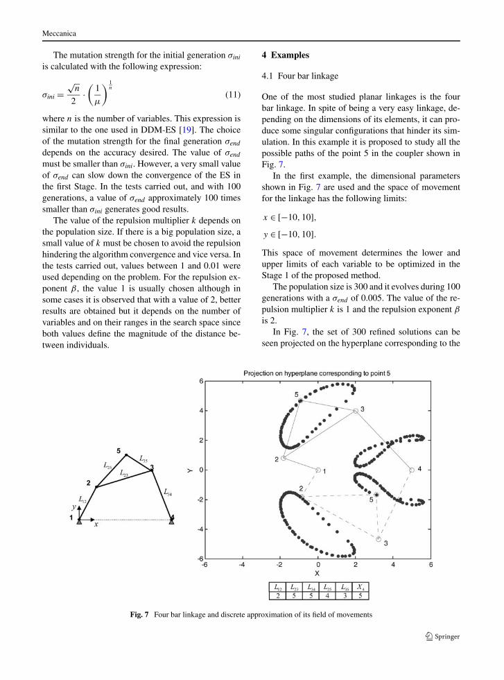
4.1 Four bar linkage

One of the most studied planar linkages is the fourbar linkage. In spite of being a very easy linkage, de-pending on the dimensions of its elements, it can pro-duce some singular configurations that hinder its sim-ulation. In this example it is proposed to study all thepossible paths of the point 5 in the coupler shown inFig. 7.

In the first example, the dimensional parametersshown in Fig. 7 are used and the space of movementfor the linkage has the following limits:

x ∈ [−10,10],y ∈ [−10,10].This space of movement determines the lower andupper limits of each variable to be optimized in theStage 1 of the proposed method.

The population size is 300 and it evolves during 100generations with a σend of 0.005. The value of the re-pulsion multiplier k is 1 and the repulsion exponent β

is 2.In Fig. 7, the set of 300 refined solutions can be

seen projected on the hyperplane corresponding to the

Fig. 7 Four bar linkage and discrete approximation of its field of movements

Meccanica

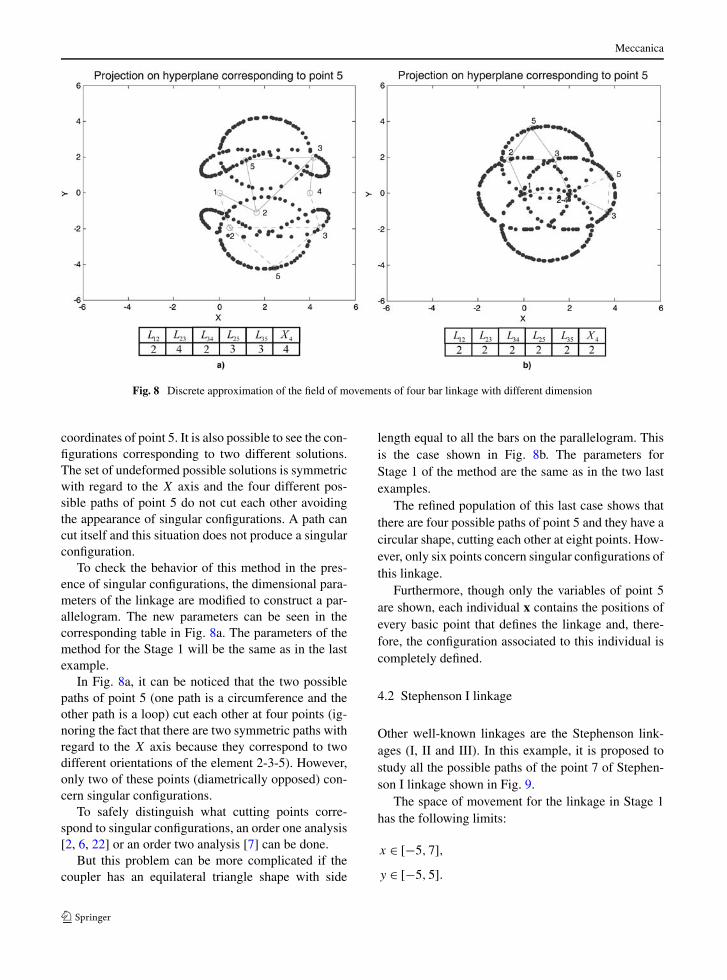
Fig. 8 Discrete approximation of the field of movements of four bar linkage with different dimension

coordinates of point 5. It is also possible to see the con-figurations corresponding to two different solutions.The set of undeformed possible solutions is symmetricwith regard to the X axis and the four different pos-sible paths of point 5 do not cut each other avoidingthe appearance of singular configurations. A path cancut itself and this situation does not produce a singularconfiguration.

To check the behavior of this method in the pres-ence of singular configurations, the dimensional para-meters of the linkage are modified to construct a par-allelogram. The new parameters can be seen in thecorresponding table in Fig. 8a. The parameters of themethod for the Stage 1 will be the same as in the lastexample.

In Fig. 8a, it can be noticed that the two possiblepaths of point 5 (one path is a circumference and theother path is a loop) cut each other at four points (ig-noring the fact that there are two symmetric paths withregard to the X axis because they correspond to twodifferent orientations of the element 2-3-5). However,only two of these points (diametrically opposed) con-cern singular configurations.

To safely distinguish what cutting points corre-spond to singular configurations, an order one analysis[2, 6, 22] or an order two analysis [7] can be done.

But this problem can be more complicated if thecoupler has an equilateral triangle shape with side

length equal to all the bars on the parallelogram. Thisis the case shown in Fig. 8b. The parameters forStage 1 of the method are the same as in the two lastexamples.

The refined population of this last case shows thatthere are four possible paths of point 5 and they have acircular shape, cutting each other at eight points. How-ever, only six points concern singular configurations ofthis linkage.

Furthermore, though only the variables of point 5are shown, each individual x contains the positions ofevery basic point that defines the linkage and, there-fore, the configuration associated to this individual iscompletely defined.

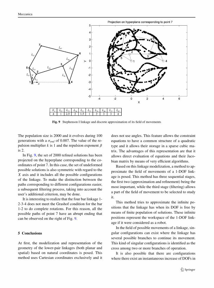
4.2 Stephenson I linkage

Other well-known linkages are the Stephenson link-ages (I, II and III). In this example, it is proposed tostudy all the possible paths of the point 7 of Stephen-son I linkage shown in Fig. 9.

The space of movement for the linkage in Stage 1has the following limits:

x ∈ [−5,7],y ∈ [−5,5].

Meccanica

Fig. 9 Stephenson I linkage and discrete approximation of its field of movements

The population size is 2000 and it evolves during 100generations with a σend of 0.007. The value of the re-pulsion multiplier k is 1 and the repulsion exponent β

is 2.In Fig. 9, the set of 2000 refined solutions has been

projected on the hyperplane corresponding to the co-ordinates of point 7. In this case, the set of undeformedpossible solutions is also symmetric with regard to theX axis and it includes all the possible configurationsof the linkage. To make the distinction between thepaths corresponding to different configurations easier,a subsequent filtering process, taking into account theuser’s additional criterion, may be done.

It is interesting to realize that the four bar linkage 1-2-3-4 does not meet the Grashof condition for the bar1-2 to do complete rotations. For this reason, all thepossible paths of point 7 have an abrupt ending thatcan be observed on the right of Fig. 9.

5 Conclusions

At first, the modelization and representation of thegeometry of the lower-pair linkages (both planar andspatial) based on natural coordinates is posed. Thismethod uses Cartesian coordinates exclusively and it

does not use angles. This feature allows the constraintequations to have a common structure of a quadratictype and it allows their storage in a sparse cubic ma-trix. The advantages of this representation are that itallows direct evaluation of equations and their Jaco-bian matrix by means of very efficient algorithms.

Based on this linkage modelization, a method to ap-proximate the field of movements of a 1-DOF link-age is posed. This method has three sequential stages,the first two (approximation and refinement) being themost important, while the third stage (filtering) allowsa part of the field of movement to be selected to studyit.

This method tries to approximate the infinite po-sitions that the linkage has when its DOF is free bymeans of finite population of solutions. These infinitepositions represent the workspace of the 1-DOF link-age if it were considered as a robot.

In the field of possible movements of a linkage, sin-gular configurations can exist where the linkage hasseveral possible branches to continue its movement.This kind of singular configurations is identified as thecross among two or more branches of operation.

It is also possible that there are configurationswhere there exist an instantaneous increase of DOFs in

Meccanica

the linkage. This type of configuration generates newbranches of operation for a part of the linkage.

Finally, there are singular configurations in whichthe linkage is blocked. This type of configurations isidentified as the end of a branch of operation of thelinkage.

These types of singular configurations are usuallystudied in the case of the workspace of robots and ma-nipulators but they do not arouse much attention in thecase of 1-DOF linkages.

The method proposed is immune to the existenceof these singular configurations and it facilitates thelocation of some of them by means of the visualizationof the complete field of movements of the linkage.

Another possible utility of the complete field ofmovements of a 1-DOF linkage is in dimensional syn-thesis of path generation. If you have a linkage withcertain dimensions, it is possible to obtain, in onego, all possible paths for the point studied and, then,search for the one that best approximates to the pathdesired. Furthermore, the type of configuration can bediscriminated by means of a filtering process. For in-stance, it is possible to define the orientation whichevery part of the linkage must have.

Another advantage of the method proposed is thatit allows the position problem to be completely dis-connected from the velocity and acceleration problemssince the field of movements of a linkage does not de-pend on the time or on the initial conditions of thesimulation as occurs in the outcomes derived from thekinematic simulation approaches.

This method has been tested on two different well-known linkages, the four bar linkage and the Stephen-son I linkage, confirming that the method is immune tothe existence of the different types of singular config-urations cited before and representing a new valid toolto detect the complete workspace of a 1-DOF linkage.

References

1. Allgower EL, Georg K (1980) Simplicial and continuationmethods for approximations, fixed points and solutions tosystems of equations. SIAM Rev 22:28–85

2. Altuzarra O, Pinto C, Avilés R, Hernández A (2004)A practical procedure to analyze singular configurations inclosed kinematic chains. IEEE Trans Robot 20(6):929–940

3. Avilés R, Ajuria MBG, Hormaza MV, Hernández A (1996)A procedure base on finite elements for the solution of non-linear problems in the kinematic analysis of mechanisms.Finite Elem Anal Des 22:305–327

4. Avilés R, Hernández A, Amezua E, Altuzarra O (2008)Kinematic analysis of linkages based in finite elementsand the geometric stiffness matrix. Mech Mach Theory43(8):964–983

5. Dennis JE Jr (1977) Nonlinear least-squares. In: State ofthe art in numerical analysis. Academic Press, New York,pp 269–312

6. Di Gregorio R (2007) A novel geometric and analytic tech-nique for the singularity analysis of one-dof planar mecha-nisms. Mech Mach Theory 42:1462–1483

7. Fernández de Bustos I, Agirrebeitia J, Avilés R, Ajuria G(2009) Second order analysis of the mobility of kinematicloops via acceleration compatibility analysis. Mech MachTheory 44(10):1923–1937

8. García de Jalón J (2007) Twenty-five years of natural coor-dinates. Multibody Syst Dyn 18(1):15–33

9. García de Jalón J, Bayo E (1994) Kinematic and dynamicsimulation of multibody systems. The real-time challenge.Springer, New York

10. Goldberg DE (1989) Genetic algorithms in search, op-timization, and machine learning. Addison-Wesley, NewYork

11. Golubitsky, Schaeffer (1985) Singularities and groups inbifurcation theory, vol 1. Springer, Berlin

12. Golubitsky, Stewart, Schaeffer (1988) Singularities andgroups in bifurcation theory, vol 2. Springer, Berlin

13. Grosan C, Abraham A (2008) A new approach for solvingnonlinear equations systems. IEEE Trans Syst Man CybernA 38(3):698–714

14. Konak A, Coit DW, Smith AE (2006) Multi-objective op-timization using genetic algorithms: a tutorial. Reliab EngSyst Saf 91:992–1007

15. Moré JJ (1977) The Levenberg-Marquardt algorithm: im-plementation and theory. Lect Notes Math 630:105–116

16. Morgan A (1987) Solving polynomial systems using con-tinuation for engineering and scientific problems. Prentice-Hall, Englewood Cliffs

17. Nocedal J, Wright SJ (1999) Numerical optimization.Springer series in operations research. Springer, New York

18. Noriega A (2008) Síntesis dimensional óptima de mecanis-mos mediante estrategias evolutivas. PhD thesis, Universityof Oviedo

19. Noriega A, Rodríguez E, Cortizo JL, Vijande R, Sierra JM(2008) A new evolution strategy for the unconstrained opti-mization problem. In: Proceedings of second internationalconference on multidisciplinary design optimization andapplications, Gijón, Spain, 3–5 September 2008

20. Schwefel HP (1995) Evolution and optimum seeking. Wi-ley, New York

21. Snyman JA (2005) Practical mathematical optimization: anintroduction to basic optimization theory and classical andnew gradient-based algorithms. Springer, New York

22. Yang D-C, Xiong J, Yang X-D (2008) A simple methodto calculate mobility with Jacobian. Mech Mach Theory43:1175–1185

23. Zlatanov D, Fenton RG, Benhabib B (1998) Identificationand classification of the singular configurations of mecha-nisms. Mech Mach Theory 33(6):743–760