A ‘high-pressure economy’ canhelp boost productivity andprovide even more ‘room torun’ for the recoveryReport • By Josh Bivens • March 10, 2017

• Washington, DC View this report at epi.org/118665

SECTIONS

1. Summary • 1

2. Background onproductivity and wagegrowth • 2

3. ‘Nowcasting’productivity growth isa bad idea • 4

4. Faster labor costgrowth can spurinvestment andproductivity growth • 11

5. Conclusion • 15

About the author • 16

Appendix: Some moreinformation onregressions used in thispaper • 17

Endnotes • 19

References • 19

SummaryThe last four years have seen an extraordinarily sharpdeceleration in productivity growth (the average amount ofincome generated in an hour of work in the economy). Infact it has been below 1 percent for three years. This is animportant trend for many reasons and it is cruciallyimportant that policymakers respond to it correctly. Takingthe slow productivity growth in recent years as fixed andunchangeable would be a huge policy mistake. It wouldlock in weak labor markets and keep most Americanworkers from getting the pay raises they could have gottenin a healthier economy. On the flip side, there is evidencethat pushing up wages by further reducing unemploymentwould increase productivity as businesses gain moreincentive to invest in the capital equipment and processesthat make those workers more productive.

Key findings of this report are the following:

The weakness in productivity growth in recent years ispredominantly a function of weakness in privateinvestment. Businesses are not investing in the equipmentand technology that makes workers more productive.

The main cause of the weakness in private investmentis the chronic shortfall of aggregate demand(spending by households, governments, andbusinesses), relative to the economy’s productivecapacity, lingering from the Great Recession. In otherwords, businesses are not investing in productivity-boosting equipment because their customers aren’tdemanding enough to ensure that the existingproductive capacity will be fully used.

Some potential benefit to investment from less-slackdemand in recent years was largely extinguished bythe large fall in energy prices that led to declines ininvestment in extractive industries. Given that theseprice declines have relented, low energy prices shouldno longer drag on business investment in comingyears.

The economy’s long-run potential rate of productivitygrowth is likely significantly higher than what the past few

1

years of growth would indicate.

The weakness in private investment that is driving low productivity growth will reverseif and when the slack in aggregate demand is taken up.

Most credible forecasters, both public and private, think that trend productivity growthin the U.S. economy remains well above 1 percent annually. The confidence that trendproductivity growth is higher than readings of very recent years is driven by a longempirical history of productivity growth reverting to long-run trends. This means it is abad idea to base future projections of potential productivity growth on the very nearpast.

If we take these last few years of productivity growth as given, this means the economy isquite close to full employment and policy should stop aiming to boost aggregate demand.This view is wrong, and potentially damaging if embraced by policymakers.

If the Federal Reserve decides that the economy is indeed at full employment, it willraise interest rates in an attempt to preemptively rein in inflation. But undertakingthese rate increases in the current economy—not allowing the recovery “room to run,”in Fed Chair Janet Yellen’s phrasing—could be leaving hundreds of billions of dollarsin potential output unclaimed in coming years. This is particularly true if an economygiven “room to run” was needed to restore decent rates of productivity growth.

Similarly, if the economy is seen as at full employment by fiscal policymakers, it couldlead them to underestimate the need for public investment to increase aggregatedemand and to prioritize the need to reduce federal budget deficits. But aninvestment swing toward further fiscal austerity would reverse some of the progresswe are just starting to see on wage growth for many workers (Gould 2017).

A “high-pressure economy” that eliminates the remaining demand shortfall in the U.S.economy and leads to low rates of unemployment and rapid wage growth would likelyinduce faster productivity growth. This faster productivity growth would in turn blunt muchof the potentially inflationary pressure stemming from tighter labor markets that generatedfaster wage-growth.

Both cross-country and international studies show a correlation between rising wagesand the pace of business investment. This evidence suggests that any inflationaryeffect of faster wage growth on prices could be significantly blunted by acorresponding increase in productivity growth as rising labor costs spur employers toboost capital investments and other drivers of productivity growth.

Background on productivity and wagegrowthProductivity is defined as the average income or output generated in an hour of work inthe economy. This makes it the ceiling to how much average living standards can rise overthe long run in an economy. It is important to note that inflation-adjusted (or real) wages

2

and incomes for the large majority of American workers and families have risensignificantly slower than economy-wide productivity growth in recent decades. Thisdivergence between a typical worker’s pay and economy-wide productivity is the rootcause of the rise in income and wage inequality over that period.

The unequal distribution of the benefits of productivity growth is an extremely importantissue. But even apart from the distribution issue, the rate of productivity growth remains acrucially important macroeconomic variable to track, not least because it provides anupper bound on how fast wages (both nominal and real) can rise.

In the 12 months ending in December 2016, nominal (or not inflation-adjusted) hourlywages rose 2.5 percent (EPI 2017). This is a bit above the pace of nominal wage growthover most of the recovery that began in June 2009, but still far below what the growth rateshould be in a healthy economy. Bivens (2014) defines a healthy-economy target fornominal wage growth as the sum of the inflation target of the Federal Reserve (2 percent)plus the trend growth of potential productivity. In that paper, it is assumed that the long-runtrend in potential productivity growth is 1.5 percent. This inflation target and an assumptionof 1.5 percent trend productivity growth establishes a nominal wage growth target of 3.5percent for a healthy economy, and actually implies that a bit faster growth is needed untilall slack in the labor market is wrung out.

The logic is easy enough to explain. If nominal wages are growing at or beneath the rateof productivity growth, then labor costs put no upward pressure on prices at all. Say thatproductivity (how much output is produced in an hour of work) rises 1 percent and nominalwages rise 1 percent. What has happened to the cost of producing 1 unit of output?Nothing. Yes, firms have to pay 1 percent more for each hour of work, but they get 1percent more output in that hour of work, so, costs per unit of output remain unchanged.

And, of course, the Federal Reserve does not target zero growth in output costs (orprices), instead it targets 2 percent growth. So, adding this 2 percent price inflation targetto productivity growth gives a pace of nominal wage growth consistent with labor costsputting no upward (or downward) pressure on the Fed’s price inflation target.

Slowing productivity growth in recent yearsIn recent years, however, measured productivity growth has come in well below 1.5percent. In fact, over the past three years, it has even been below 1 percent. Figure Ashows the three-year moving average of productivity growth. The rapid, recentdeceleration is obvious in this series (look at the big dip on the far right of the line).However, this recently poor performance of productivity should not lead us to significantlyratchet down our estimate of long-run potential productivity growth.

The first reason not to lower our estimate of long-run productivity growth is thatproductivity growth is a volatile economic data series even over a 3-year horizon. In partbecause of this well-known fact, very few economic forecasters have radically markeddown their estimates of trend productivity growth in recent years. The CongressionalBudget Office (CBO), for example, in its latest Budget and Economic Outlook (CBO 2017)

3

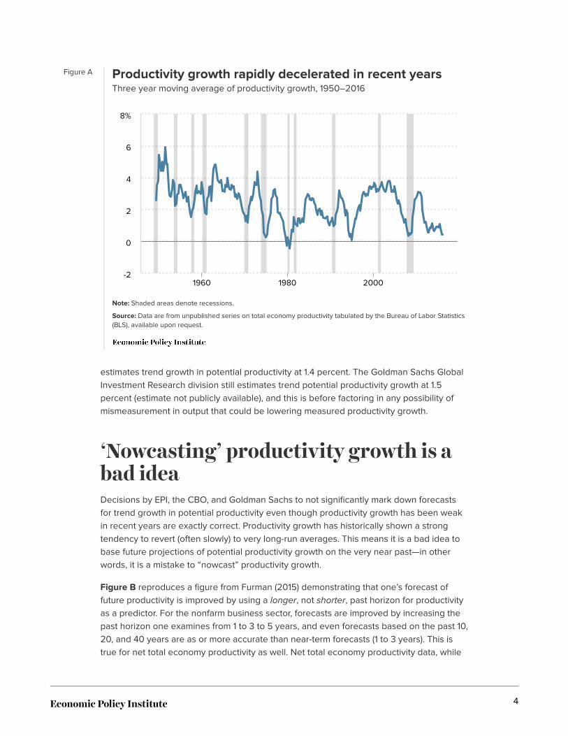
Figure A Productivity growth rapidly decelerated in recent yearsThree year moving average of productivity growth, 1950–2016

Note: Shaded areas denote recessions.

Source: Data are from unpublished series on total economy productivity tabulated by the Bureau of Labor Statistics(BLS), available upon request.

-2

0

2

4

6

8%

1960 1980 2000

estimates trend growth in potential productivity at 1.4 percent. The Goldman Sachs GlobalInvestment Research division still estimates trend potential productivity growth at 1.5percent (estimate not publicly available), and this is before factoring in any possibility ofmismeasurement in output that could be lowering measured productivity growth.

‘Nowcasting’ productivity growth is abad ideaDecisions by EPI, the CBO, and Goldman Sachs to not significantly mark down forecastsfor trend growth in potential productivity even though productivity growth has been weakin recent years are exactly correct. Productivity growth has historically shown a strongtendency to revert (often slowly) to very long-run averages. This means it is a bad idea tobase future projections of potential productivity growth on the very near past—in otherwords, it is a mistake to “nowcast” productivity growth.

Figure B reproduces a figure from Furman (2015) demonstrating that one’s forecast offuture productivity is improved by using a longer, not shorter, past horizon for productivityas a predictor. For the nonfarm business sector, forecasts are improved by increasing thepast horizon one examines from 1 to 3 to 5 years, and even forecasts based on the past 10,20, and 40 years are as or more accurate than near-term forecasts (1 to 3 years). This istrue for net total economy productivity as well. Net total economy productivity data, while

4

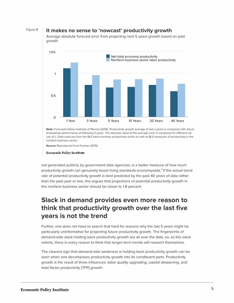
Figure B It makes no sense to ‘nowcast’ productivity growthAverage absolute forecast error from projecting next 5 years growth based on pastgrowth

Note: Forecasts follow methods of Mericle (2016). Productivity growth average of last x years is compared with actualproductivity performance of following 5 years. The absolute value of the average error is compared for different val-ues of x. Data used are from the BLS total economy productivity series as well as BLS measures of productivity in thenonfarm business sector.

Source: Reproduced from Furman (2015)

Net total economy productivityNonfarm business sector labor productivity

1 Year 3 Years 5 Years 10 Years 20 Years 40 Years0

0.5

1

1.5%

not generated publicly by government data agencies, is a better measure of how muchproductivity growth can genuinely boost living standards economywide.1 If the actual trendrate of potential productivity growth is best predicted by the past 40 years of data ratherthan the past year or two, this argues that projections of potential productivity growth inthe nonfarm business sector should be closer to 1.8 percent.

Slack in demand provides even more reason tothink that productivity growth over the last fiveyears is not the trendFurther, one does not have to search that hard for reasons why the last 5 years might beparticularly uninformative for projecting future productivity growth. The fingerprints ofdemand-side slack holding back productivity growth are all over the data, so, as this slackrelents, there is every reason to think that longer-term trends will reassert themselves.

The clearest sign that demand-side weakness is holding back productivity growth can beseen when one decomposes productivity growth into its constituent parts. Productivitygrowth is the result of three influences: labor quality upgrading, capital deepening, andtotal factor productivity (TFP) growth.

5

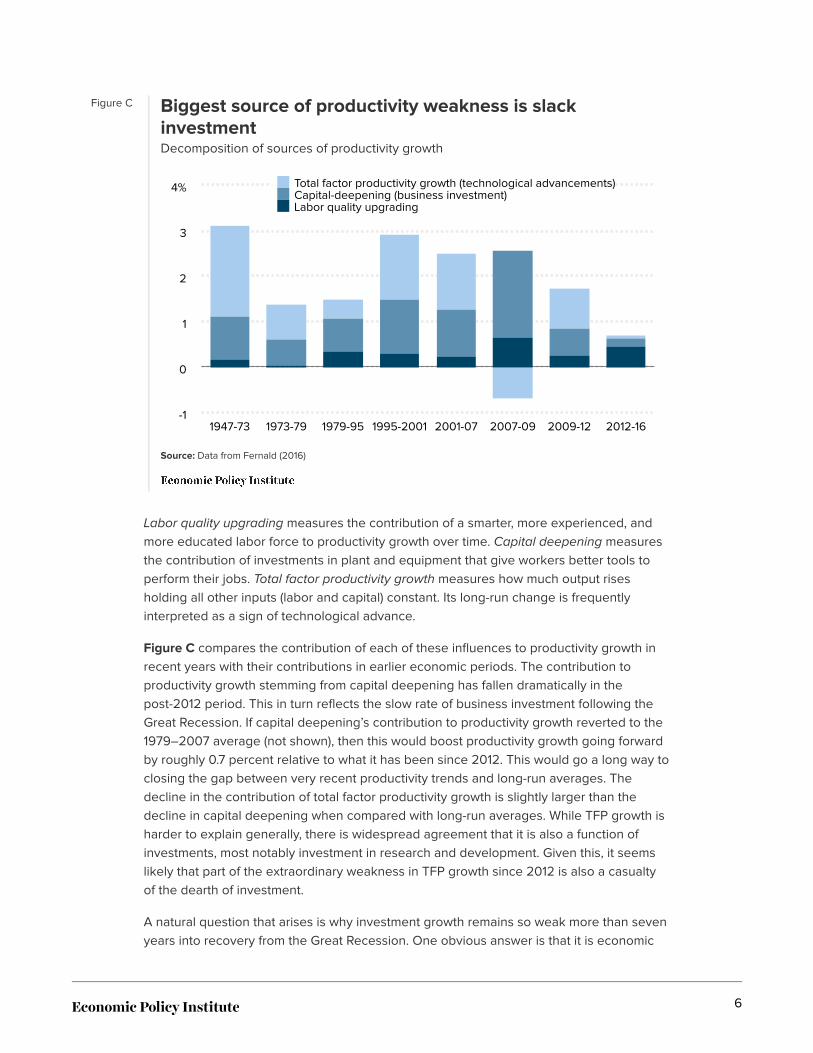
Figure C Biggest source of productivity weakness is slackinvestmentDecomposition of sources of productivity growth

Source: Data from Fernald (2016)

Total factor productivity growth (technological advancements)Capital-deepening (business investment)Labor quality upgrading

-1

0

1

2

3

4%

1947-73 1973-79 1979-95 1995-2001 2001-07 2007-09 2009-12 2012-16

Labor quality upgrading measures the contribution of a smarter, more experienced, andmore educated labor force to productivity growth over time. Capital deepening measuresthe contribution of investments in plant and equipment that give workers better tools toperform their jobs. Total factor productivity growth measures how much output risesholding all other inputs (labor and capital) constant. Its long-run change is frequentlyinterpreted as a sign of technological advance.

Figure C compares the contribution of each of these influences to productivity growth inrecent years with their contributions in earlier economic periods. The contribution toproductivity growth stemming from capital deepening has fallen dramatically in thepost-2012 period. This in turn reflects the slow rate of business investment following theGreat Recession. If capital deepening’s contribution to productivity growth reverted to the1979–2007 average (not shown), then this would boost productivity growth going forwardby roughly 0.7 percent relative to what it has been since 2012. This would go a long way toclosing the gap between very recent productivity trends and long-run averages. Thedecline in the contribution of total factor productivity growth is slightly larger than thedecline in capital deepening when compared with long-run averages. While TFP growth isharder to explain generally, there is widespread agreement that it is also a function ofinvestments, most notably investment in research and development. Given this, it seemslikely that part of the extraordinary weakness in TFP growth since 2012 is also a casualtyof the dearth of investment.

A natural question that arises is why investment growth remains so weak more than sevenyears into recovery from the Great Recession. One obvious answer is that it is economic

6

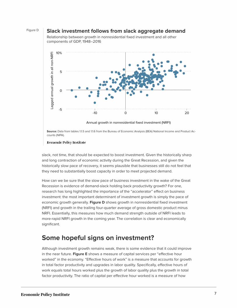
Figure D Slack investment follows from slack aggregate demandRelationship between growth in nonresidential fixed investment and all othercomponents of GDP, 1948–2016

Source: Data from tables 1.1.5 and 1.1.6 from the Bureau of Economic Analysis (BEA) National Income and Product Ac-counts (NIPA).

Annual growth in nonresidential fixed investment (NRFI)

Lagg

ed a

nnua

l gro

wth

in a

ll no

n-N

RFI

-10 0 10 20-5

0

5

10%

slack, not time, that should be expected to boost investment. Given the historically sharpand long contraction of economic activity during the Great Recession, and given thehistorically slow pace of recovery, it seems plausible that businesses still do not feel thatthey need to substantially boost capacity in order to meet projected demand.

How can we be sure that the slow pace of business investment in the wake of the GreatRecession is evidence of demand-slack holding back productivity growth? For one,research has long highlighted the importance of the “accelerator” effect on businessinvestment: the most important determinant of investment growth is simply the pace ofeconomic growth generally. Figure D shows growth in nonresidential fixed investment(NRFI) and growth in the trailing four-quarter average of gross domestic product minusNRFI. Essentially, this measures how much demand strength outside of NRFI leads tomore-rapid NRFI growth in the coming year. The correlation is clear and economicallysignificant.

Some hopeful signs on investment?Although investment growth remains weak, there is some evidence that it could improvein the near future. Figure E shows a measure of capital services per “effective hourworked” in the economy. “Effective hours of work” is a measure that accounts for growthin total factor productivity and upgrades in labor quality. Specifically, effective hours ofwork equals total hours worked plus the growth of labor quality plus the growth in totalfactor productivity. The ratio of capital per effective hour worked is a measure of how

7

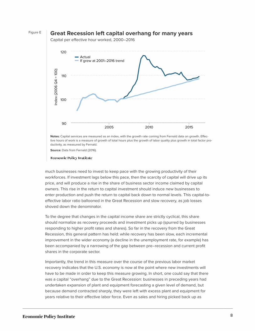
Figure E Great Recession left capital overhang for many yearsCapital per effective hour worked, 2000–2016

Notes: Capital services are measured as an index, with the growth rate coming from Fernald data on growth. Effec-tive hours of work is a measure of growth of total hours plus the growth of labor quality plus growth in total factor pro-ductivity, as measured by Fernald.

Source: Data from Fernald (2016).

Inde

x (2

00

6 Q

4 =

100

)ActualIf grew at 2001–2016 trend

20102005 201590

100

110

120

much businesses need to invest to keep pace with the growing productivity of theirworkforces. If investment lags below this pace, then the scarcity of capital will drive up itsprice, and will produce a rise in the share of business sector income claimed by capitalowners. This rise in the return to capital investment should induce new businesses toenter production and push the return to capital back down to normal levels. This capital-to-effective labor ratio ballooned in the Great Recession and slow recovery, as job lossesshoved down the denominator.

To the degree that changes in the capital income share are strictly cyclical, this shareshould normalize as recovery proceeds and investment picks up (spurred by businessesresponding to higher profit rates and shares). So far in the recovery from the GreatRecession, this general pattern has held: while recovery has been slow, each incrementalimprovement in the wider economy (a decline in the unemployment rate, for example) hasbeen accompanied by a narrowing of the gap between pre–recession and current profitshares in the corporate sector.

Importantly, the trend in this measure over the course of the previous labor marketrecovery indicates that the U.S. economy is now at the point where new investments willhave to be made in order to keep this measure growing. In short, one could say that therewas a capital “overhang” due to the Great Recession: businesses in preceding years hadundertaken expansion of plant and equipment forecasting a given level of demand, butbecause demand contracted sharply, they were left with excess plant and equipment foryears relative to their effective labor force. Even as sales and hiring picked back up as

8

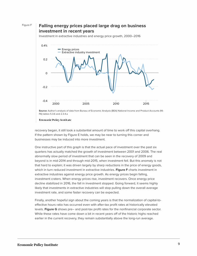
Figure F Falling energy prices placed large drag on businessinvestment in recent yearsInvestment in extractive industries and energy price growth, 2000–2016

Source: Author’s analysis of data from Bureau of Economic Analysis (BEA) National Income and Product Accounts (NI-PA) tables 5.3.6 and 2.3.4.a

Energy pricesExtractive industry investment

-0.4

-0.2

0

0.2

0.4%

2000 2005 2010 2015

recovery began, it still took a substantial amount of time to work off this capital overhang.If the pattern shown by Figure E holds, we may be near to turning this corner andbusinesses may be induced into more investment.

One instructive part of this graph is that the actual pace of investment over the past sixquarters has actually matched the growth of investment between 2001 and 2006. The realabnormally slow period of investment that can be seen in the recovery of 2009 andbeyond is in mid-2014 and through mid-2015, when investment fell. But this anomaly is notthat hard to explain; it was driven largely by sharp reductions in the price of energy goods,which in turn reduced investment in extractive industries. Figure F charts investment inextractive industries against energy price growth. As energy prices begin falling,investment craters. When energy prices rise, investment recovers. Once energy pricedecline stabilized in 2016, the fall in investment stopped. Going forward, it seems highlylikely that investments in extractive industries will stop pulling down the overall averageinvestment rate, and some faster recovery can be expected.

Finally, another hopeful sign about the coming years is that the normalization of capital-to-effective hours ratio has occurred even with after-tax profit rates at historically elevatedlevels. Figure G shows pre– and post-tax profit rates for the nonfinancial corporate sector.While these rates have come down a bit in recent years off of the historic highs reachedearlier in the current recovery, they remain substantially above the long-run average.

9

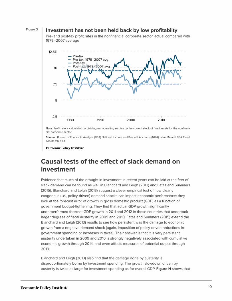
Figure G Investment has not been held back by low profitabiltyPre- and post-tax profit rates in the nonfinancial corporate sector, actual compared with1979–2007 average

Note: Profit rate is calculated by dividing net operating surplus by the current stock of fixed assets for the nonfinan-cial corporate sector.

Source: Bureau of Economic Analysis (BEA) National Income and Product Accounts (NIPA) table 1.14 and BEA FixedAssets table 4.1

Pre-taxPre-tax, 1979–2007 avgPost-taxPost-tax, 1979–2007 avg

1980 1990 2000 2010

10

2.5

5

7.5

12.5%

Causal tests of the effect of slack demand oninvestmentEvidence that much of the drought in investment in recent years can be laid at the feet ofslack demand can be found as well in Blanchard and Leigh (2013) and Fatas and Summers(2015). Blanchard and Leigh (2013) suggest a clever empirical test of how clearlyexogenous (i.e., policy-driven) demand shocks can impact economic performance: theylook at the forecast error of growth in gross domestic product (GDP) as a function ofgovernment budget-tightening. They find that actual GDP growth significantlyunderperformed forecast GDP growth in 2011 and 2012 in those countries that undertooklarger degrees of fiscal austerity in 2009 and 2010. Fatas and Summers (2015) extend theBlanchard and Leigh (2013) results to see how persistent was the damage to economicgrowth from a negative demand shock (again, imposition of policy-driven reductions ingovernment spending or increases in taxes). Their answer is that it is very persistent:austerity undertaken in 2009 and 2010 is strongly negatively associated with cumulativeeconomic growth through 2014, and even affects measures of potential output through2019.

Blanchard and Leigh (2013) also find that the damage done by austerity isdisproportionately borne by investment spending. The growth slowdown driven byausterity is twice as large for investment spending as for overall GDP. Figure H shows that

10

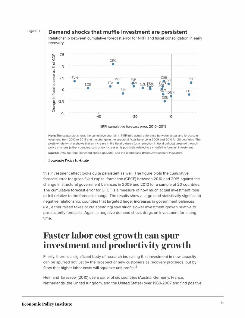
Figure H Demand shocks that muffle investment are persistentRelationship between cumulative forecast error for NRFI and fiscal consolidation in earlyrecovery

Note: The scatterplot shows the cumulative shortfall in NRFI (the actual difference between actual and forecast in-vestment) from 2010 to 2015 and the change in the structural fiscal balance in 2009 and 2010 for 20 countries. Thepositive relationship shows that an increase in the fiscal balance (or a reduction in fiscal deficits) targeted throughpolicy changes (either spending cuts or tax increases) is positively related to a shortfall in forecast investment.

Source: Data are from Blanchard and Leigh (2013) and the World Bank World Development Indicators.

NRFI cumulative forecast error, 2010–2015

Cha

nge

in fi

scal

bal

ance

as

% o

f GD

P

AUT

BELBGR CAN

CHE

CZE

DEUDNK

ESP

FINFRA

GBR

GRC

ITA JPNNLDPRT SVKSVN

USA

-40 -20 0-5

-2.5

0

2.5

5

7.5

this investment effect looks quite persistent as well. The figure plots the cumulativeforecast error for gross fixed capital formation (GFCF) between 2010 and 2015 against thechange in structural government balances in 2009 and 2010 for a sample of 20 countries.The cumulative forecast error for GFCF is a measure of how much actual investment roseor fell relative to the forecast change. The results show a large (and statistically significant)negative relationship: countries that targeted larger increases in government balances(i.e., either raised taxes or cut spending) saw much slower investment growth relative topre-austerity forecasts. Again, a negative demand shock drags on investment for a longtime.

Faster labor cost growth can spurinvestment and productivity growthFinally, there is a significant body of research indicating that investment in new capacitycan be spurred not just by the prospect of new customers as recovery proceeds, but byfears that higher labor costs will squeeze unit profits.2

Hein and Tarassow (2010) use a panel of six countries (Austria, Germany, France,Netherlands, the United Kingdom, and the United States) over 1960-2007 and find positive

11

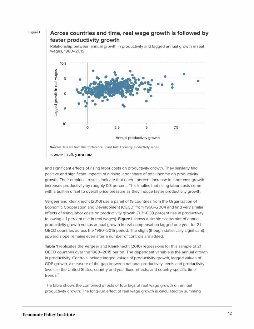
Figure I Across countries and time, real wage growth is followed byfaster productivity growthRelationship between annual growth in productivity and lagged annual growth in realwages, 1980–2015

Source: Data are from the Conference Board Total Economy Productivity series.

Annual productivity growth

Lagg

ed g

row

th in

rea

l wag

es

0 2.5 5 7.5-10

-5

0

5

10%

and significant effects of rising labor costs on productivity growth. They similarly findpositive and significant impacts of a rising labor share of total income on productivitygrowth. Their empirical results indicate that each 1 percent increase in labor cost growthincreases productivity by roughly 0.3 percent. This implies that rising labor costs comewith a built-in offset to overall price pressure as they induce faster productivity growth.

Vergeer and Kleinknecht (2010) use a panel of 19 countries from the Organization ofEconomic Cooperation and Development (OECD) from 1960–2004 and find very similareffects of rising labor costs on productivity growth (0.31-0.39 percent rise in productivityfollowing a 1 percent rise in real wages). Figure I shows a simple scatterplot of annualproductivity growth versus annual growth in real compensation lagged one year for 21OECD countries across the 1980–2015 period. The slight (though statistically significant)upward slope remains even after a number of controls are added.

Table 1 replicates the Vergeer and Kleinknecht (2010) regressions for this sample of 21OECD countries over the 1980–2015 period. The dependent variable is the annual growthin productivity. Controls include lagged values of productivity growth, lagged values ofGDP growth, a measure of the gap between national productivity levels and productivitylevels in the United States, country and year fixed-effects, and country-specific time-trends.3

The table shows the combined effects of four lags of real wage growth on annualproductivity growth. The long-run effect of real wage growth is calculated by summing

12

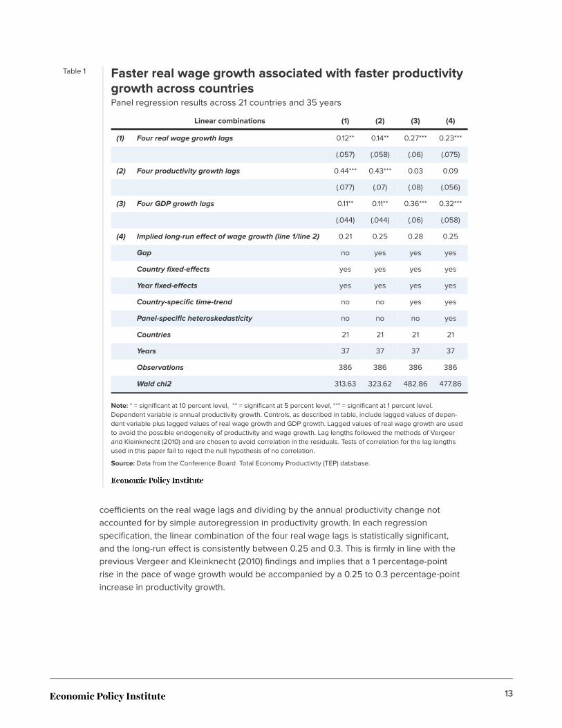
Table 1 Faster real wage growth associated with faster productivitygrowth across countriesPanel regression results across 21 countries and 35 years

Linear combinations (1) (2) (3) (4)

(1) Four real wage growth lags 0.12** 0.14** 0.27*** 0.23***

(.057) (.058) (.06) (.075)

(2) Four productivity growth lags 0.44*** 0.43*** 0.03 0.09

(.077) (.07) (.08) (.056)

(3) Four GDP growth lags 0.11** 0.11** 0.36*** 0.32***

(.044) (.044) (.06) (.058)

(4) Implied long-run effect of wage growth (line 1/line 2) 0.21 0.25 0.28 0.25

Gap no yes yes yes

Country fixed-effects yes yes yes yes

Year fixed-effects yes yes yes yes

Country-specific time-trend no no yes yes

Panel-specific heteroskedasticity no no no yes

Countries 21 21 21 21

Years 37 37 37 37

Observations 386 386 386 386

Wald chi2 313.63 323.62 482.86 477.86

Note: * = significant at 10 percent level, ** = significant at 5 percent level, *** = significant at 1 percent level.Dependent variable is annual productivity growth. Controls, as described in table, include lagged values of depen-dent variable plus lagged values of real wage growth and GDP growth. Lagged values of real wage growth are usedto avoid the possible endogeneity of productivity and wage growth. Lag lengths followed the methods of Vergeerand Kleinknecht (2010) and are chosen to avoid correlation in the residuals. Tests of correlation for the lag lengthsused in this paper fail to reject the null hypothesis of no correlation.

Source: Data from the Conference Board Total Economy Productivity (TEP) database.

coefficients on the real wage lags and dividing by the annual productivity change notaccounted for by simple autoregression in productivity growth. In each regressionspecification, the linear combination of the four real wage lags is statistically significant,and the long-run effect is consistently between 0.25 and 0.3. This is firmly in line with theprevious Vergeer and Kleinknecht (2010) findings and implies that a 1 percentage-pointrise in the pace of wage growth would be accompanied by a 0.25 to 0.3 percentage-pointincrease in productivity growth.

13

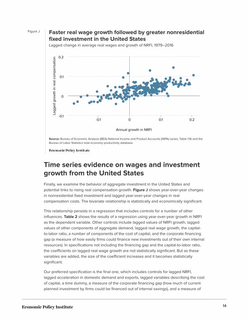
Figure J Faster real wage growth followed by greater nonresidentialfixed investment in the United StatesLagged change in average real wages and growth of NRFI, 1979–2016

Source: Bureau of Economic Analysis (BEA) National Income and Product Accounts (NIPA) series, Table 1.16 and theBureau of Labor Statistics total economy productivity database.

Annual growth in NRFI

Lagg

ed g

row

th in

rea

l com

pens

atio

n

-0.1 0 0.1 0.2-0.1

0

0.1

0.2

Time series evidence on wages and investmentgrowth from the United StatesFinally, we examine the behavior of aggregate investment in the United States andpotential links to rising real compensation growth. Figure J shows year-over-year changesin nonresidential fixed investment and lagged year-over-year changes in realcompensation costs. The bivariate relationship is statistically and economically significant.

This relationship persists in a regression that includes controls for a number of otherinfluences. Table 2 shows the results of a regression using year-over-year growth in NRFIas the dependent variable. Other controls include lagged values of NRFI growth, laggedvalues of other components of aggregate demand, lagged real wage growth, the capital-to-labor ratio, a number of components of the cost of capital, and the corporate financinggap (a measure of how easily firms could finance new investments out of their own internalresources). In specifications not including the financing gap and the capital-to-labor ratio,the coefficients on lagged real wage growth are not statistically significant. But as thesevariables are added, the size of the coefficient increases and it becomes statisticallysignificant.

Our preferred specification is the final one, which includes controls for lagged NRFI,lagged acceleration in domestic demand and exports, lagged variables describing the costof capital, a time dummy, a measure of the corporate financing gap (how much of currentplanned investment by firms could be financed out of internal savings), and a measure of

14

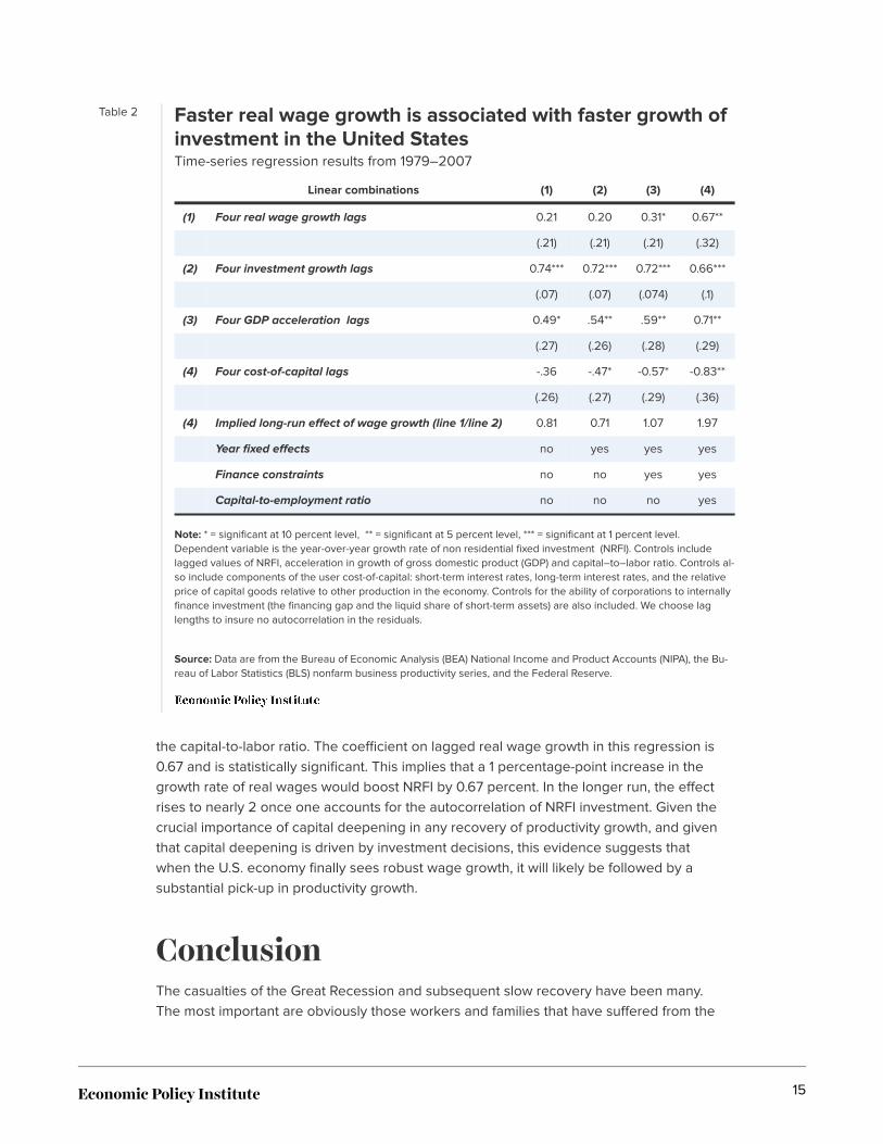
Table 2 Faster real wage growth is associated with faster growth ofinvestment in the United StatesTime-series regression results from 1979–2007

Linear combinations (1) (2) (3) (4)

(1) Four real wage growth lags 0.21 0.20 0.31* 0.67**

(.21) (.21) (.21) (.32)

(2) Four investment growth lags 0.74*** 0.72*** 0.72*** 0.66***

(.07) (.07) (.074) (.1)

(3) Four GDP acceleration lags 0.49* .54** .59** 0.71**

(.27) (.26) (.28) (.29)

(4) Four cost-of-capital lags -.36 -.47* -0.57* -0.83**

(.26) (.27) (.29) (.36)

(4) Implied long-run effect of wage growth (line 1/line 2) 0.81 0.71 1.07 1.97

Year fixed effects no yes yes yes

Finance constraints no no yes yes

Capital-to-employment ratio no no no yes

Note: * = significant at 10 percent level, ** = significant at 5 percent level, *** = significant at 1 percent level.Dependent variable is the year-over-year growth rate of non residential fixed investment (NRFI). Controls includelagged values of NRFI, acceleration in growth of gross domestic product (GDP) and capital–to–labor ratio. Controls al-so include components of the user cost-of-capital: short-term interest rates, long-term interest rates, and the relativeprice of capital goods relative to other production in the economy. Controls for the ability of corporations to internallyfinance investment (the financing gap and the liquid share of short-term assets) are also included. We choose laglengths to insure no autocorrelation in the residuals.

Source: Data are from the Bureau of Economic Analysis (BEA) National Income and Product Accounts (NIPA), the Bu-reau of Labor Statistics (BLS) nonfarm business productivity series, and the Federal Reserve.

the capital-to-labor ratio. The coefficient on lagged real wage growth in this regression is0.67 and is statistically significant. This implies that a 1 percentage-point increase in thegrowth rate of real wages would boost NRFI by 0.67 percent. In the longer run, the effectrises to nearly 2 once one accounts for the autocorrelation of NRFI investment. Given thecrucial importance of capital deepening in any recovery of productivity growth, and giventhat capital deepening is driven by investment decisions, this evidence suggests thatwhen the U.S. economy finally sees robust wage growth, it will likely be followed by asubstantial pick-up in productivity growth.

ConclusionThe casualties of the Great Recession and subsequent slow recovery have been many.The most important are obviously those workers and families that have suffered from the

15

loss of jobs and declining wages and incomes. But another casualty of the GreatRecession is a deceleration of productivity growth. Given that productivity growth providesthe ceiling on how fast potential living standards can rise, it is crucially important to notaccept a lower rate of productivity growth if it can be fixed by policy.

And one key driver of slow productivity growth in recent years can be fixed: the remainingshortfall between aggregate demand and the economy’s productive potential. Running theeconomy far below potential for a long time has led to insufficient investment to sustainrapid productivity growth. One way to close this accumulated investment gap is, of course,to simply have fiscal policymakers boost public investment. And this should indeed be aresponse.

But another crucial response is to ensure that the labor market and wider economy run hotenough to force businesses to boost investment simply to meet growing demand. Whenthis is done, policymakers also need to keep the recovery strong until real wages beginconsistently rising. From a policy perspective this means keeping interest rates low andnot prematurely raising them due to misguided fears of inflation. The inflationary impact ofa pick-up in real wages is likely to be quite muffled by the faster investment andproductivity growth that will follow.

As with all macroeconomic predictions, this one about productivity rising to meet wagegrowth could be wrong. But the downside risk of being wrong is relatively small; a coupleof years of above-target price inflation as wages push up costs. Given the many years ofbelow-target inflation, one hesitates to even call this a “downside” of a policy that has theeconomy going for growth. The downside risk of reining in demand before we even testthe virtuous cycle of rising wages leading to rising productivity growth, however, isenormous. The decline in potential output for 2017 between what was forecast in 2007and what is estimated now is almost $2 trillion. If half of this—$1 trillion—could be clawedback through a policy that runs the economy hot and leads to higher productivity growth, itwill be an extraordinarily consequential policy choice.

About the authorJosh Bivens joined the Economic Policy Institute in 2002 and is currently the director ofresearch. His primary areas of research include macroeconomics, social insurance, andglobalization. He has authored or co-authored three books (including The State of WorkingAmerica, 12th Edition) while working at EPI, edited another, and has written numerousresearch papers, including for academic journals. He often appears in media outlets tooffer economic commentary and has testified several times before the U.S. Congress. Heearned his Ph.D. from The New School for Social Research.

16

Appendix: Some more information onregressions used in this paperWe use three regression analyses in this paper. The first replicates the tests of Fatas andSummers (2015) on the persistent impact of fiscal consolidation (increasing thegovernment’s structural budget balance) on economic growth. We then use investment,rather than overall gross domestic product (GDP), as our dependent variable. The datacome from the Blanchard and Leigh (2013) extract from the IMF World Economic Outlookfrom 2010 (IMF 2010). In this version of the World Economic Outlook, the IMF forecasts anumber of variables five years ahead. We then use actual data on investment from theWorld Bank’s World Development Indicators database to compare actual versus forecastnonresidential fixed investment between 2010 and 2015. We then correlate the differencebetween actual and forecast investment (or, the “forecast error”) with the change in thestructural fiscal balance in 2009 and 2010. As the scatterplot in Figure H shows, there is asystematic association between fiscal consolidation (cutting spending or raising taxes) anda large, negative forecast error. Following Blanchard and Leigh (2013) and Fatas andSummers (2015), we interpret this association as the causal effect of an exogenous shock(a clear policy decision to cut budget deficits) on subsequent investment growth. Wepicked the countries to include in our sample to match the Fatas and Summers (2015)sample.

The second regression analysis is based on panel data consisting of 21 advancedcountries over the 1980-2015 period. The data includes the Conference Board’s TotalEconomy Productivity (TEP) database. The TEP includes data on labor productivity growth,output, employment, total hours, and total compensation. We undertook this regression toassess whether or not the results found by Vergeer and Kleinknecht (2010) held with moreup-to-date data.

In each case the dependent variable is the average annual change in productivity. Ourbaseline regression uses lags of the dependent variable, GDP growth, and year andcountry-specific fixed-effects as controls. Four lags of real wage growth are used asdependent variables as well. For lagged variables, the coefficient and standard errors ofthe linear combination of all lags are reported in Table 1. The real wage growth is enteredwith lags to avoid endogeneity problems in correlating with productivity growth. Also,given that a prime mechanism through which firms may boost productivity in response torapid labor cost growth is investment in either capital equipment or better processes(which would boost total factor productivity growth), it makes sense that such investmentcomes online only after some lag.

We follow the guidance of Vergeer and Kleinknecht (2010) in choosing lags based oneliminating serial correlation in our results. Including four lags leads to a failure to rejectthe hypothesis of no serial correlation in the residuals.

Other versions of the regression include country-specific time trends, a variable measuringhow far a country’s productivity level is from the United States, and a regression thatallows for panel-specific heteroskedasticity. The coefficient on lagged real wage growth is

17

consistently statistically significant in all regression specifications, and in the one with allcontrols is economically significant as well. We follow Hein and Tarassow (2010) inexpressing the long-run effect of lagged real wage growth as summing up the coefficientson these and dividing by one minus the summed coefficients of the lagged endogenousvariables.

While the precise estimate of the coefficients on lagged real wage growth changes withdecisions on lags, and its statistical significance is often outside conventional levels, theestimated coefficient (or sum of coefficients) is uniformly positive. Further, the pattern isclear that adding lags from 1 to 4 monotonically increases the estimated sum ofcoefficients. Given the general difficulty in establishing durable estimating relationshipsfrom cross-country macroeconomic panel data, the positive influence of real wage growthon productivity strikes us as durable.

A final regression analysis, based loosely on specifications used by Tevlin and Whelan(2000), uses quarterly macroeconomic data from the United States since 1979. Weundertook this to assess the impact of rising wages on the pace of investment. Thedependent variable in this regression is year-over-year growth in nonresidential fixedinvestment from the Bureau of Economic Analysis National Income and Product Accountsdata. Control variables include lagged dependent variables, lagged year-over-yearchanges in growth rates for all elements of foreign and domestic demand besides NRFI,variables that influence the cost of capital investment to firms (the effective federal fundsrate, which is a short-term interest rate controlled by the Federal Reserve; the interest rateon 10-year Treasury bonds; and the relative price of capital goods), measures of internalcorporate financing capability (the “financing gap,” which is a computation of capitalexpenditures minus corporate profits, and the share of all assets held in short-term liquidforms), measure of the ratio of the aggregate capital stock to overall employment (thecapital-to-labor ratio), and year fixed-effects.

We again use four lags on each variable, but since we are now using quarterly data, thisimplies a much shorter effect. We again follow the Vergeer and Kleinknecht (2010)standard of including lags until there is no evidence of serial correlation. Further, we usethe year-long lag to account for previous studies’ findings that the effects of someinfluences on investment (interest rates, for example) take this long to filter through intochanges in investment trends.

When not including controls on internal financing constraints or year fixed-effects, the sumof coefficients on real compensation growth is statistically insignificant. However, in thepreferred specification in which controls for internal financing, year fixed-effects, and thecurrent capital-to-labor ratio are included, the sum of lagged real wage coefficientsbecome statistically and economically significant. Further, when these lags are includedthe sum of lagged dependent variable coefficients becomes economically trivial andstatistically insignificant. This implies that the long-run impact of faster real wage growthfor increases in NRFI is considerable, with each 1 percentage-point increase in wagegrowth translating over time into a 2 percentage-point increase in the growth rate of NRFI.We should also note that the estimated effect of the cost of capital on aggregateinvestment also increases in both economic and statistical significance as further controls

18

are added.

Endnotes1. For more on net, economy–wide productivity, see Bivens and Mishel (2015).

2. Key examples of a theoretical treatment of this include Bhaduri (2003), Dutt (2006), Barbosa-Filho(2004) , and Barbosa-Filho and Taylor (2006).

3. Some more details about the data and methods used in regression analyses in this paper can befound in the appendix.

ReferencesBarbosa-Filho, Nelson. 2004. “A Simple Model of Demand-Led Growth and Income Distribution.”Working Paper. Institute of Economics, Federal University of Rio de Janeiro, Brazil.

Barbosa-Filho, Nelson, and Lance Taylor. 2006. “Distributive and Demand Cycles in the U.S.Economy: A Structuralist Goodwin Model.” Metroeconomica, vol. 57, no. 3, 289–411.

Bhaduri, Amit. 2003. “Alternative Approaches to Endogenous Growth.” Working Paper. JawaharlalNehru University, India.

Bivens, Josh. 2014. A Vital Dashboard Indicator for Monetary Policy: Nominal Wage Targets. PolicyFutures Project, Center for Budget and Policy Priorities.

Bivens, Josh, and Lawrence Mishel. 2015. Understanding the Historic Divergence betweenProductivity and a Typical Worker’s Pay: Why It Matters and Why It’s Real. Economic Policy Institute.

Blanchard, Olivier, and Daniel Leigh. 2013. “Growth Forecast Errors and Fiscal Multipliers.” WorkingPaper. International Monetary Fund.

Bureau of Economic Analysis (BEA). Fixed Assets Tables. Various years. Fixed Asset Tables 4.1.

Bureau of Economic Analysis (BEA). National Income and Product Accounts (NIPA). Various years.National Income and Product Accounts Tables [data tables].

Bureau of Labor Statistics (BLS) (U.S. Department of Labor) Labor Productivity and Costs program.Various years. Major Sector Productivity and Costs and Industry Productivity and Costs [databases].http://www.bls.gov/lpc/#data. (Unpublished data provided by program staff at EPI’s request.)

Conference Board. 2016. Total Economy Productivity (TEP) database, November 2016.

Congressional Budget Office (CBO). 2017. Budget and Economic Outlook, 2017 to 2027.

Dutt, Amitava. 2006. “Aggregate Demand, Aggregate Supply and Economic Growth.” InternationalReview of Applied Economics, vol. 20, no. 3, 319–336.

Economic Policy Institute (EPI). 2017. “Nominal Wage Tracker.” Updated February 17.

Fatas, Antonio, and Lawrence Summers. 2015. “The Permanent Effects of Fiscal Consolidations.”Discussion Paper, Centre for Economic Policy Research.

19

Federal Reserve. 2016. “H.15 Release on Selected Interest Rates.” Accessed December 2016.

Fernald, John. 2016. “A Quarterly, Utilization-Adjusted Series on Total Factor Productivity.” FederalReserve Bank of San Francisco Working Paper 2012-19, updated December 2016.

Furman, Jason. 2015. “Productivity Growth in the Advanced Economies: The Past, the Present, andLessons for the Future.” Speech given at Peterson Institute for International Economics, Washington,D.C., July 9.

Gould, Elise. 2017. The State of American Wages 2016: Lower Unemployment Finally Helps WorkingPeople Make Up Some Lost Ground on Wages. Economic Policy Institute report.

Hein, Eckhard, and Artur Tarassow. 2010. “Distribution, Aggregate Demand and Productivity Growth:Theory and Empirical Results for Six OECD Countries Based On a Post-Kaleckian Model.” CambridgeJournal of Economics, vol. 34, 727–754.

International Monetary Fund (IMF). 2010. World Economic Outlook Database 2010.

Mericle, David. 2016. “Trend Productivity Growth: 2% Still Seems about Right.” Goldman-Sachs U.S.Daily (unpublished email), November.

Tevlin, Stacey, and Karl Whelan. 2000. “Explaining the Investment Boom of the 1990s.” WorkingPaper. Federal Reserve Board.

Vergeer, Robert, and Alfred Kleinknecht. 2010. “Jobs versus Productivity: The Causal Link fromWages to Labour Productivity Growth.” TU Delft Working Paper.

World Bank. Various years. World Development Indicators.

20