Embed Size (px)
Citation preview
A Deeper Look at LPV
Stephan Bohacek
USC
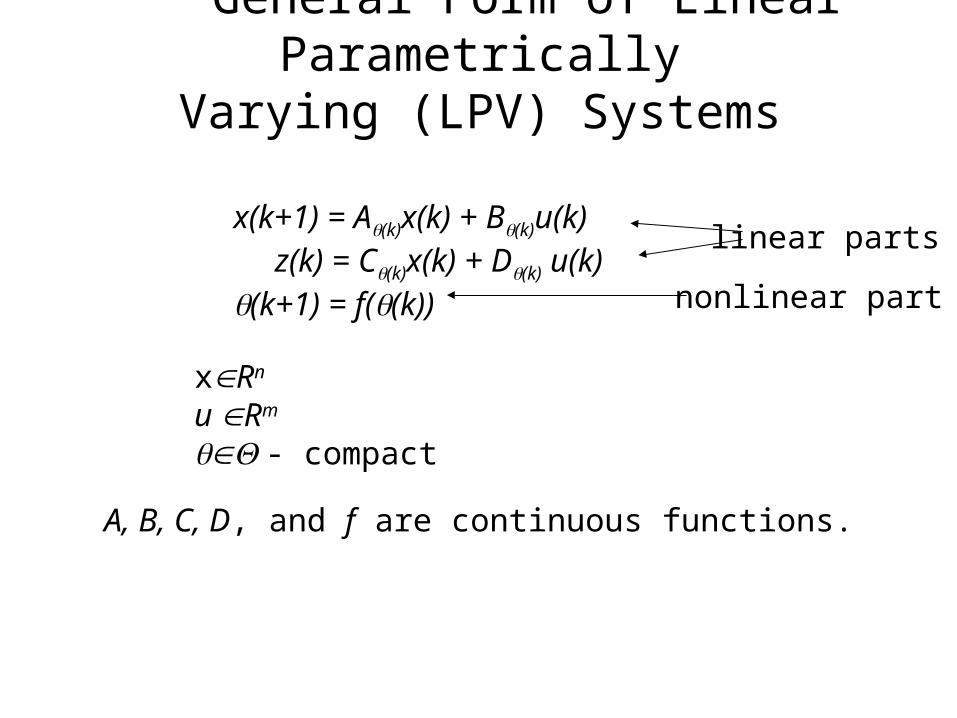
General Form of Linear ParametricallyVarying (LPV) Systems
x(k+1) = A(k)x(k) + B(k)u(k) z(k) = C(k)x(k) + D(k) u(k)(k+1) = f((k))
linear parts
nonlinear part
xRn
u Rm
- compact
A, B, C, D, and f are continuous functions.
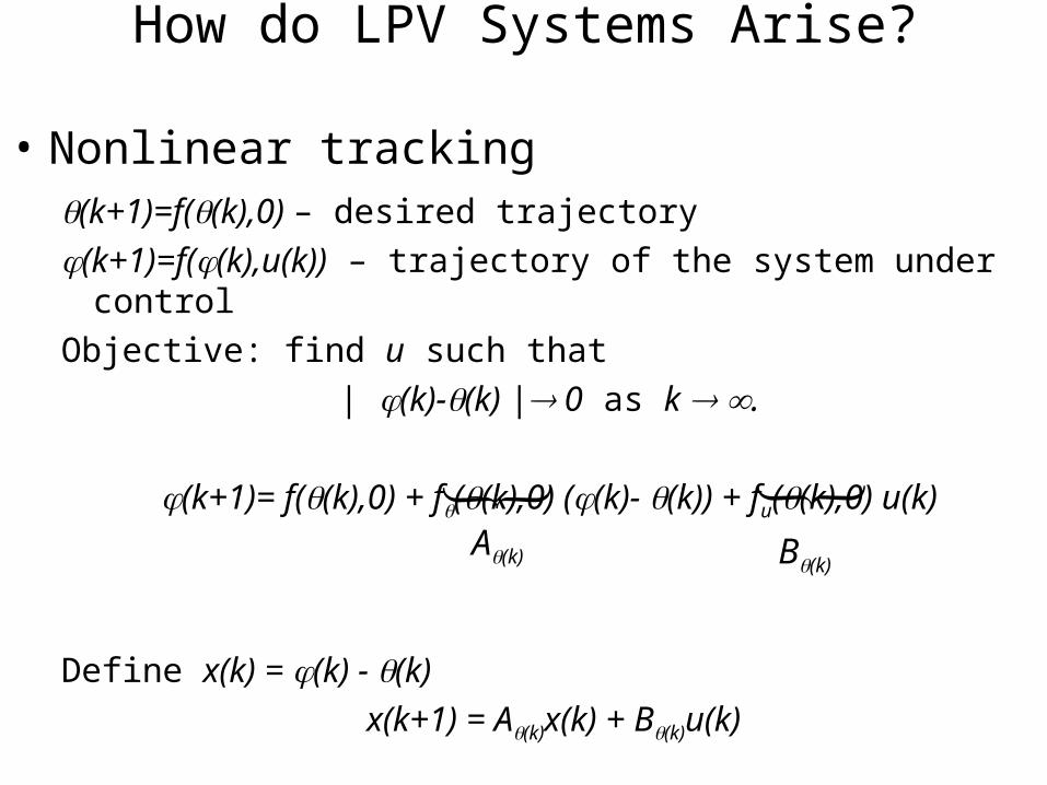
How do LPV Systems Arise?
• Nonlinear tracking(k+1)=f((k),0) – desired trajectory
(k+1)=f((k),u(k)) – trajectory of the system under control
Objective: find u such that
| (k)-(k) | 0 as k .
(k+1)= f((k),0) + f((k),0) ((k)- (k)) + fu((k),0) u(k)
Define x(k) = (k) - (k)
x(k+1) = A(k)x(k) + B(k)u(k)
A(k) B(k)
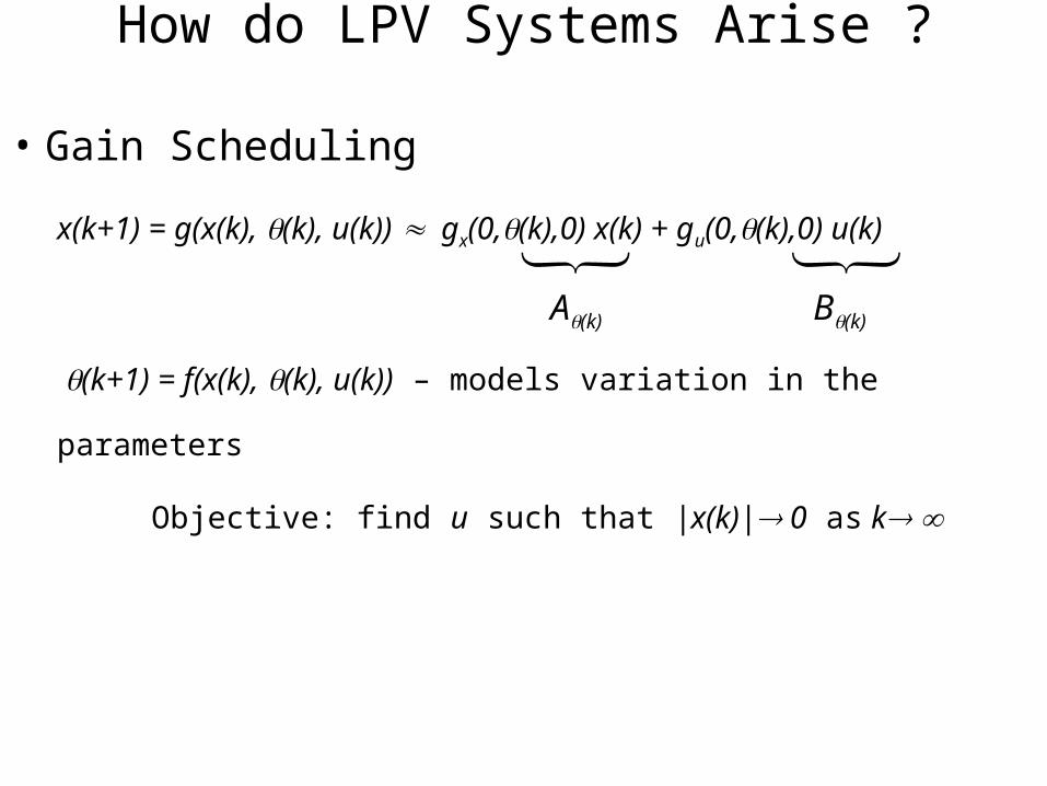
How do LPV Systems Arise ?
• Gain Scheduling
x(k+1) = g(x(k), (k), u(k)) gx(0,(k),0) x(k) + gu(0,(k),0) u(k)
(k+1) = f(x(k), (k), u(k)) – models variation in the parameters
Objective: find u such that |x(k)| 0 as k
A(k) B(k)
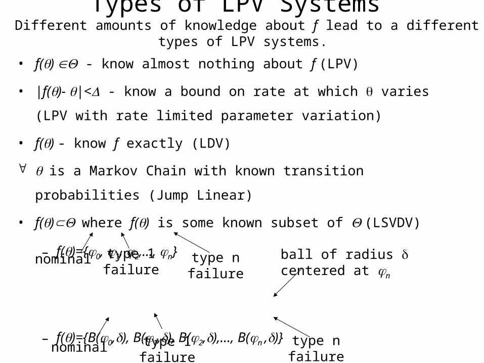
Types of LPV Systems Different amounts of knowledge about f lead to a different types of LPV systems.
• f() - know almost nothing about f (LPV)
• |f()- |< - know a bound on rate at which varies (LPV with rate limited
parameter variation)
• f() - know f exactly (LDV)
is a Markov Chain with known transition probabilities (Jump Linear)
• f() where f() is some known subset of (LSVDV)
– f()={0, 1, 2,…, n}
– f()={B(0,), B(1,), B(2,),…, B(n ,)}
nominal type 1failure
type nfailure
nominal type 1failure
type nfailure
ball of radius centered at n
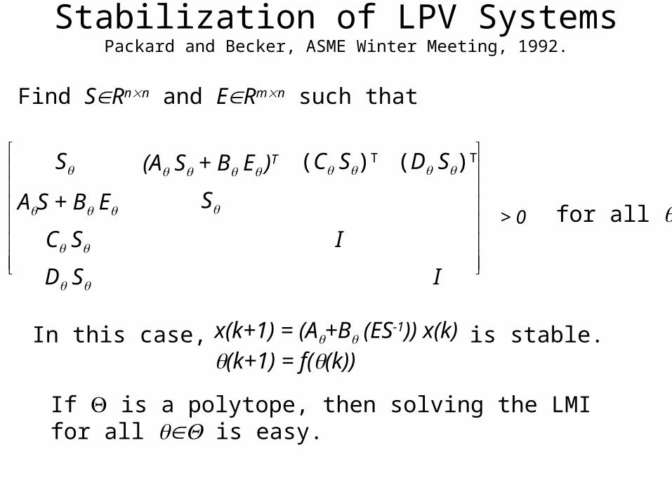
S (A S + B E )T (C S)T (D S)T
AS + B E S
C S I
D S I
Stabilization of LPV SystemsPackard and Becker, ASME Winter Meeting, 1992.
Find SRnn and ERmn such that
x(k+1) = (A+B (ES-1)) x(k)(k+1) = f((k))
In this case, is stable.
If is a polytope, then solving the LMI for all is easy.
> 0
for all
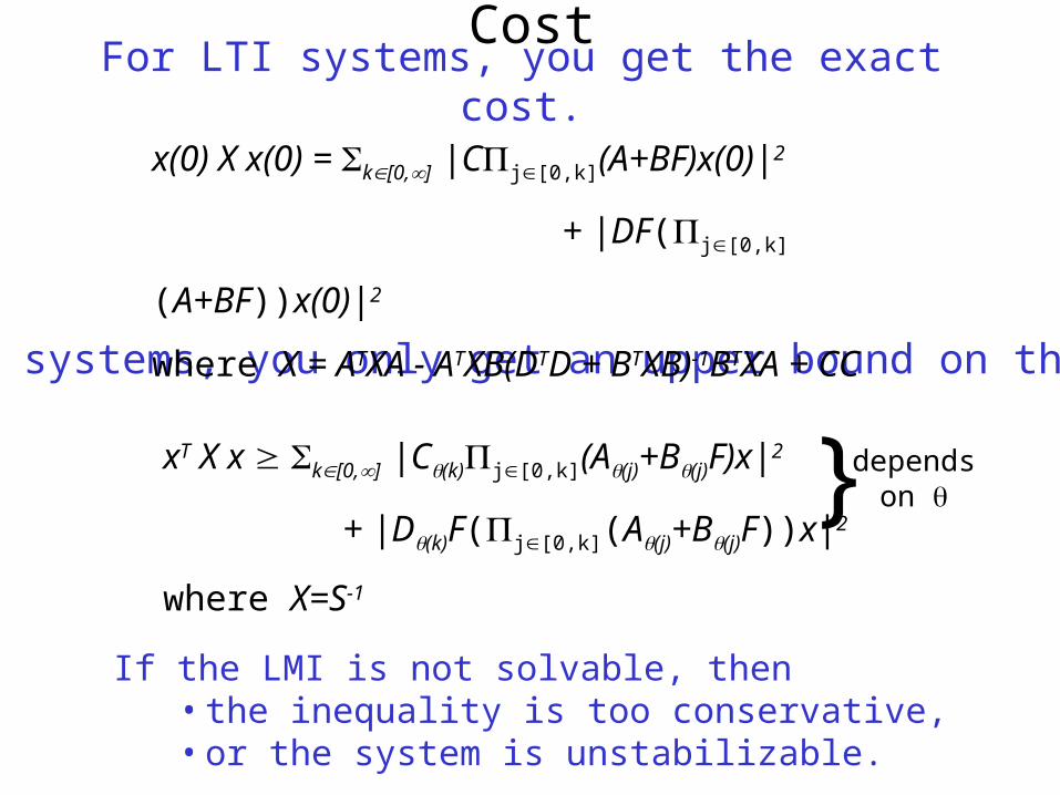
xT X x k[0,] |C(k)j[0,k](A(j)+B(j)F)x|2
+ |D(k)F(j[0,k](A(j)+B(j)F))x|2
where X=S-1
Cost
For LPV systems, you only get an upper bound on the cost.
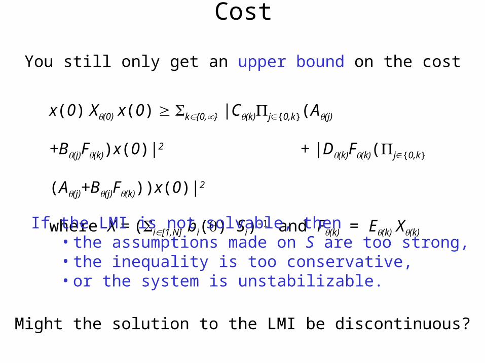
x(0) X x(0) = k[0,] |Cj[0,k](A+BF)x(0)|2
+ |DF(j[0,k](A+BF))x(0)|2
where X = ATXA - ATXB(DTD + BTXB)-1BTXA + CC
}depends on
For LTI systems, you get the exact cost.
If the LMI is not solvable, then • the inequality is too conservative,• or the system is unstabilizable.
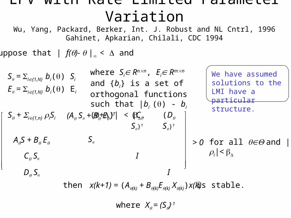
S + i{1,n} iSi (A S + B E )T (C S)T (D S)T
AS + B E S
C S I
D S I
LPV with Rate Limited Parameter VariationWu, Yang, Packard, Berker, Int. J. Robust and NL Cntrl, 1996
Gahinet, Apkarian, Chilali, CDC 1994
Suppose that | f()- | < and
S = i{1,N} bi() Si
E = i{1,N} bi() Ei
> 0 for all and |i|<
x(k+1) = (A(k) + B(k)E(k) X(k))x(k)
where X = (S)-1
then is stable.
where Si Rnn, Ei Rmn and {bi} is a set of orthogonal functions such that |bi () - bi (+)| < .
We have assumed solutions to the LMI have a particular structure.
Cost
x(0) X(0) x(0) k{0,} |C(k)j{0,k}(A(j)+B(j)F(k))x(0)|2
+ |D(k)F(k)(j{0,k}(A(j)
+B(j)F(k)))x(0)|2
where X = (i[1,N] bi() Si)-1 and F(k) = E(k) X(k)
You still only get an upper bound on the cost
Might the solution to the LMI be discontinuous?
If the LMI is not solvable, then • the assumptions made on S are too strong,• the inequality is too conservative,• or the system is unstabilizable.

|x(k+j)| (0)(0)|x(k)|
Linear Dynamically Varying (LDV) Systems Bohacek and Jonckheere, IEEE Trans. AC
Assume that f is known.
Def: The LDV system defined by (f,A,B) is stabilizable if there exists
F : Z Rmn
such that, if x(k+1) = (A(k) + B(k)F((0),k)) x(k)
(k+1) = f((k))
then j
for some (0) < and (0) < 1.
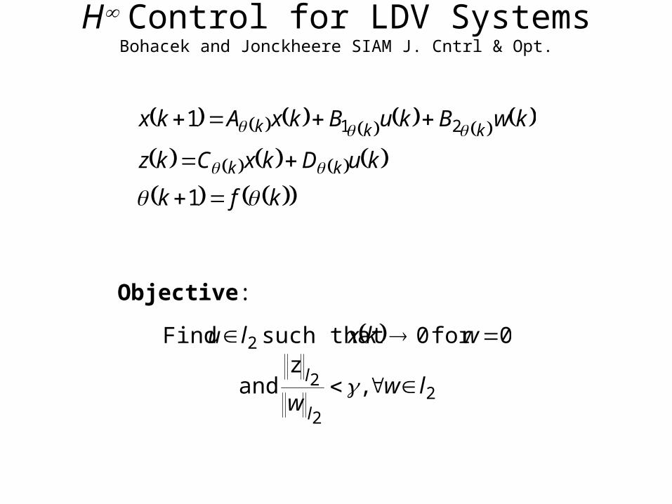
x(k+1) = A(k)x(k) + B(k)u(k) z(k) = C(k)x(k) + D(k) u(k)(k+1) = f((k))
A, B, C, D and f are continuous functions.
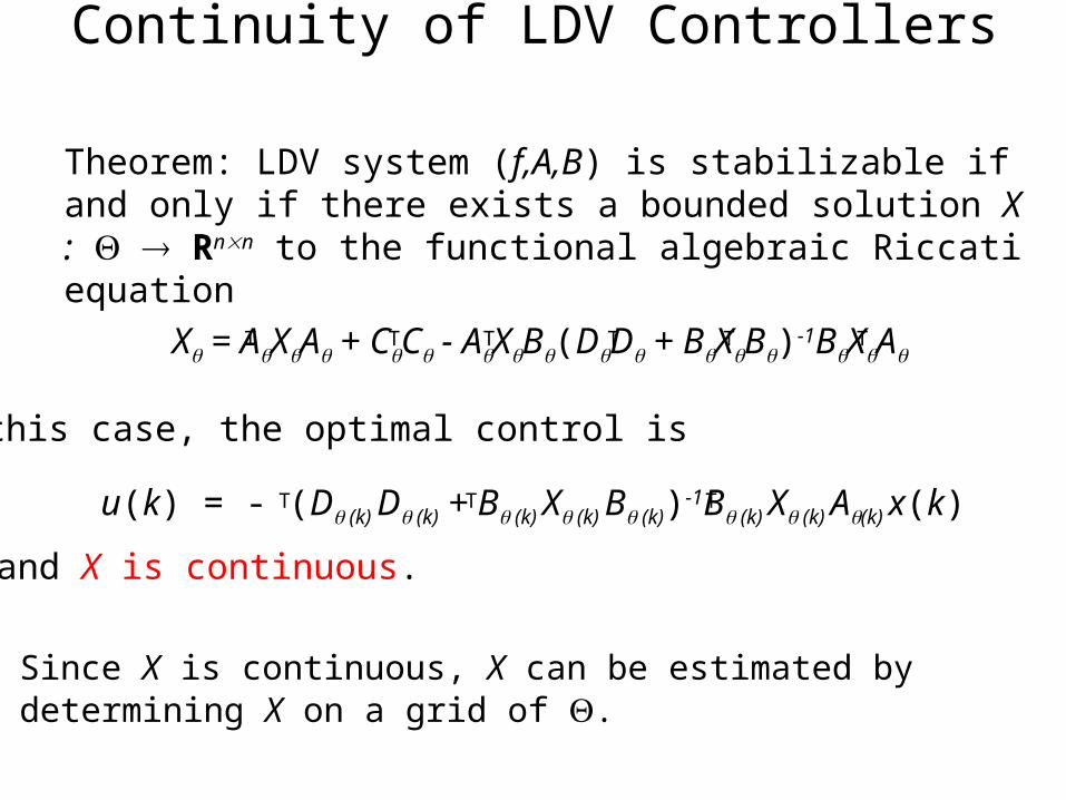
Continuity of LDV Controllers
X = AXA + CC - AXB(DD + BXB)-1BXA T T T T T T
Theorem: LDV system (f,A,B) is stabilizable if and only if there exists a bounded solution X : Rnn to the functional algebraic Riccati equation
In this case, the optimal control is
Since X is continuous, X can be estimated by determining X on a grid of .
and X is continuous.
u(k) = - (D (k) D (k) + B (k) X (k) B (k))-1B (k) X (k) A(k) x(k)T T T
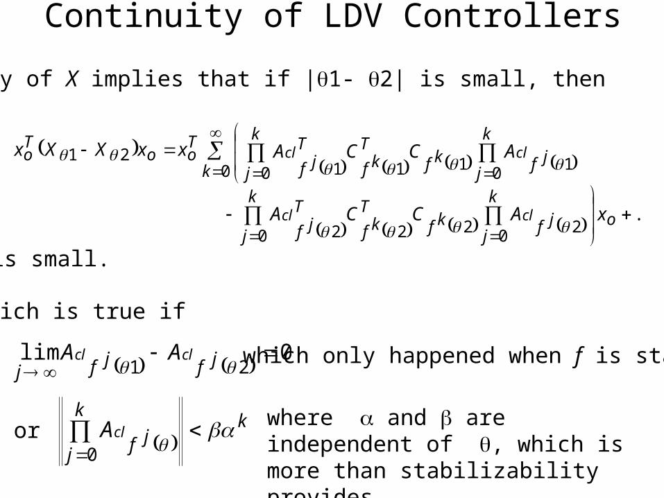
Continuity of X implies that if |1- 2| is small, then
k
jjfkf
Tkf
k
j
Tjf
clcl ACCA0
1110 1
...0
2220 2
o
k
jjfkf
Tkf
k
j
Tjf
xACCA clcl
021
k
Too
To xxXXx
which only happened when f is stable, 0lim21
jfjfjclcl AA
Which is true if
or k
k
jjf
clA
0
where and are independent of , which is more than stabilizability provides.
Continuity of LDV Controllers
is small.
kk
kkkuk
12
22
11
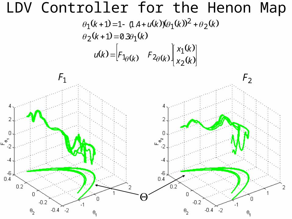
3.01
)4.1(11
LDV Controller for the Henon Map
kx
kxFFku kk
2
121
1F 2F
kfk
kuDkxCkz
kwBkuBkxAkx
kk
kkk
1
1 21
Objective:
0for 0such that Find 2 wkxlu
2
2
2 ,z
and lww l
l
H Control for LDV SystemsBohacek and Jonckheere SIAM J. Cntrl & Opt.
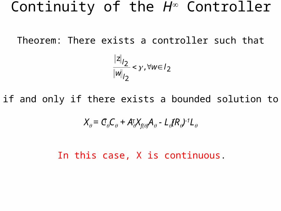
Continuity of the H Controller
Theorem: There exists a controller such that
22
2 ,z
lww l
l
if and only if there exists a bounded solution to
X = CC + AXf()A - L(R)-1L
In this case, X is continuous.
TT T
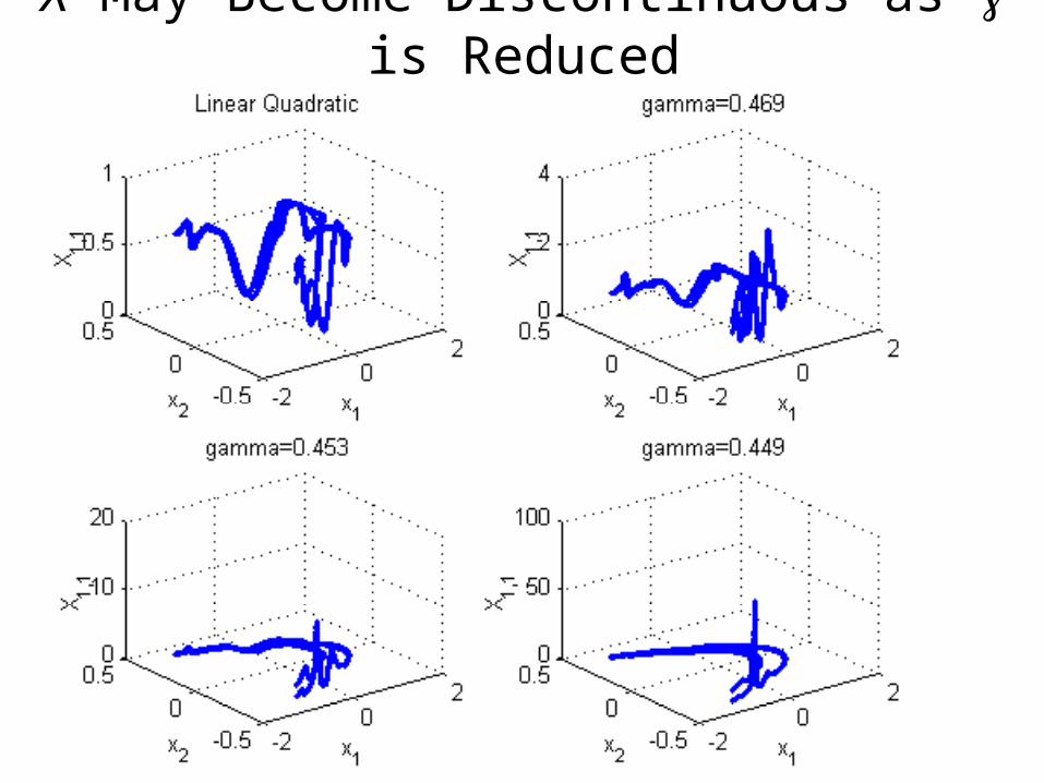
X May Become Discontinuous as is Reduced
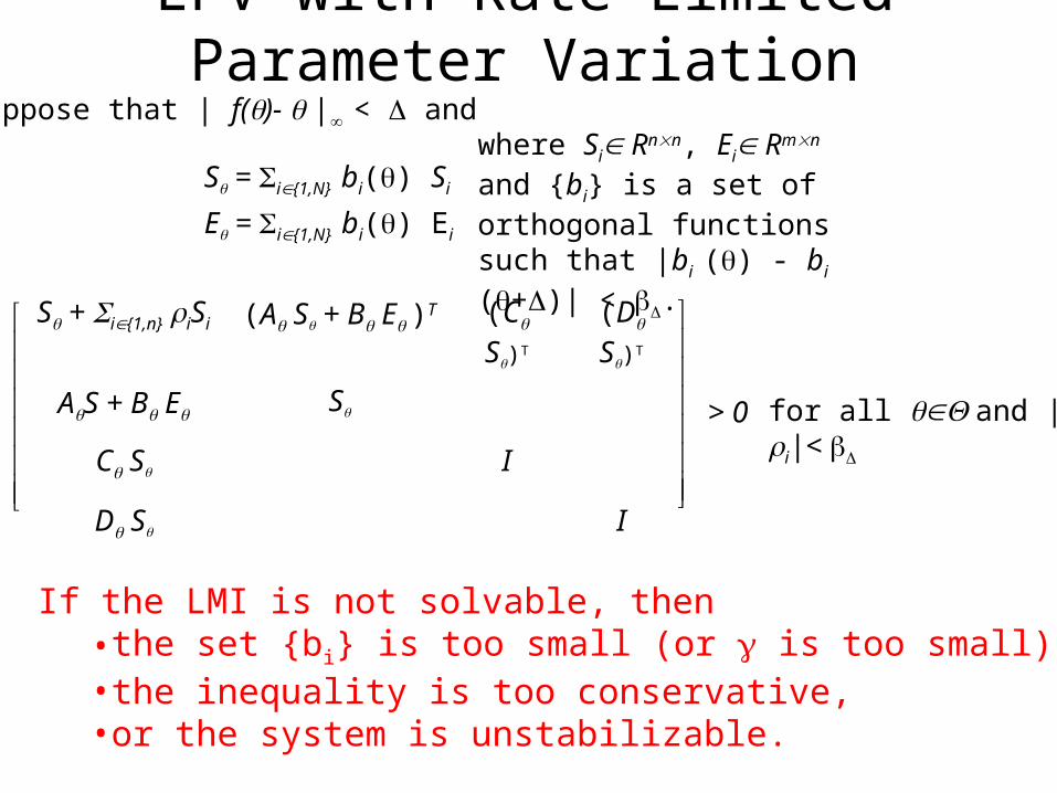
LPV with Rate Limited Parameter Variation
If the LMI is not solvable, then • the set {bi} is too small (or is too small),• the inequality is too conservative,• or the system is unstabilizable.
S + i{1,n} iSi (A S + B E )T (C S)T (D S)T
AS + B E S
C S I
D S I
Suppose that | f()- | < and
S = i{1,N} bi() Si
E = i{1,N} bi() Ei
> 0 for all and |i|<
where Si Rnn, Ei Rmn and {bi} is a set of orthogonal functions such that |bi () - bi (+)| < .
1 kfk
1
kuD
kxCkz
kuBkxAkx
k
k
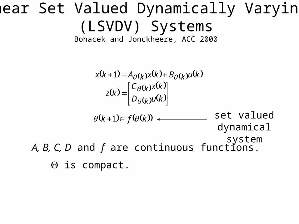
kk
Linear Set Valued Dynamically Varying (LSVDV) SystemsBohacek and Jonckheere, ACC 2000
A, B, C, D and f are continuous functions.
is compact.
set valued dynamical system
1
2
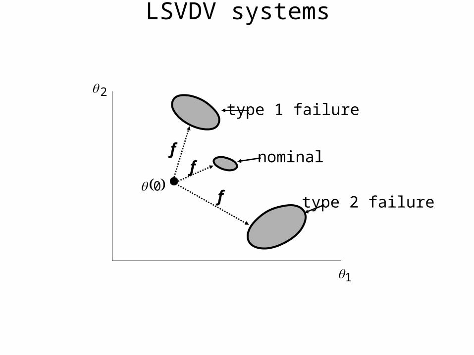
0
nominal
type 1 failure
type 2 failure
ff
f
LSVDV systems
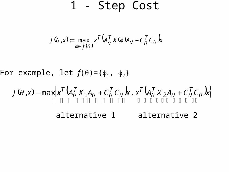
xCCAXAxxJ TTT
f
max:,
For example, let f()={1, 2}
xCCAXAxxCCAXAxxJ TTTTTT 21 ,max,
alternative 1 alternative 2
1 - Step Cost
-2 -1.5 -1 -0.5 0 0.5 1 1.5 2-2
-1.5
-1
-0.5
0
0.5
1
1.5
2
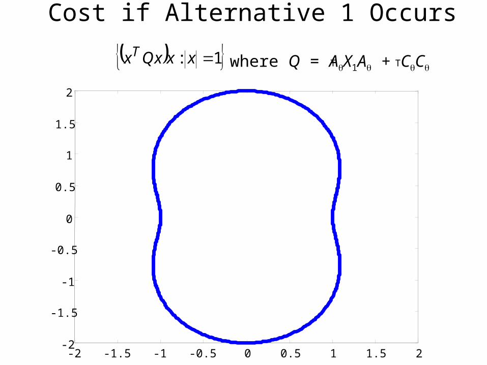
Cost if Alternative 1 Occurs
1: xxxQxTwhere Q = AX1A + CC TT
-2 -1.5 -1 -0.5 0 0.5 1 1.5 2-2
-1.5
-1
-0.5
0
0.5
1
1.5
2
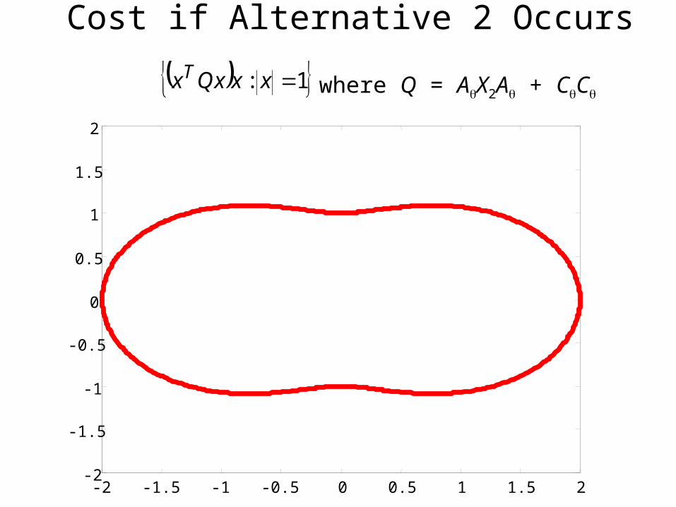
Cost if Alternative 2 Occurs
1: xxxQxTwhere Q = AX2A + CC
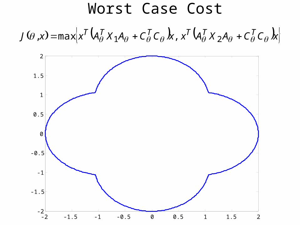
Worst Case Cost
-2 -1.5 -1 -0.5 0 0.5 1 1.5 2-2
-1.5
-1
-0.5
0
0.5
1
1.5
2
xCCAXAxxCCAXAxxJ TTTTTT 21 ,max,
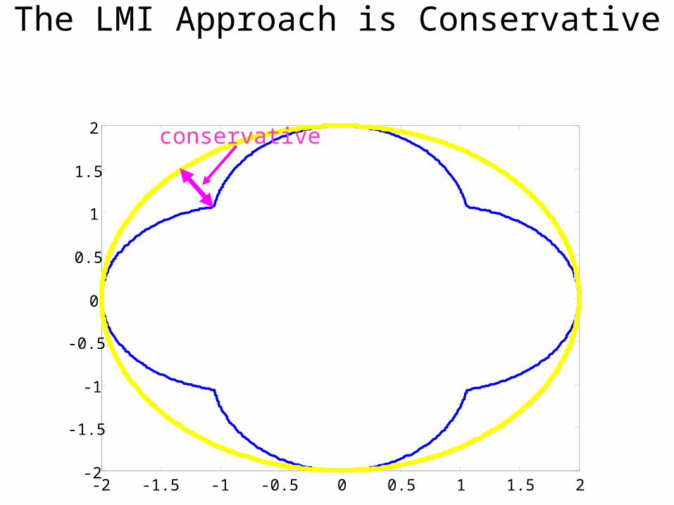
The LMI Approach is Conservative
-2 -1.5 -1 -0.5 0 0.5 1 1.5 2-2
-1.5
-1
-0.5
0
0.5
1
1.5
2 conservative
-2 -1.5 -1 -0.5 0 0.5 1 1.5 2-2
-1.5
-1
-0.5
0
0.5
1
1.5
2
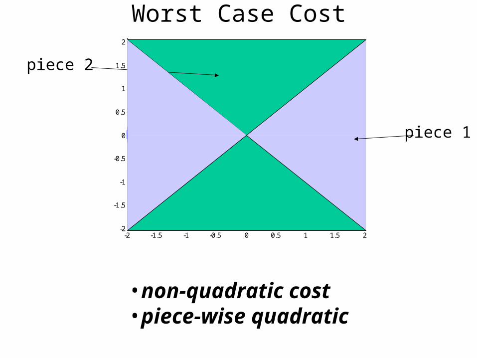
•non-quadratic cost•piece-wise quadratic
Worst Case Cost
piece 1
piece 2
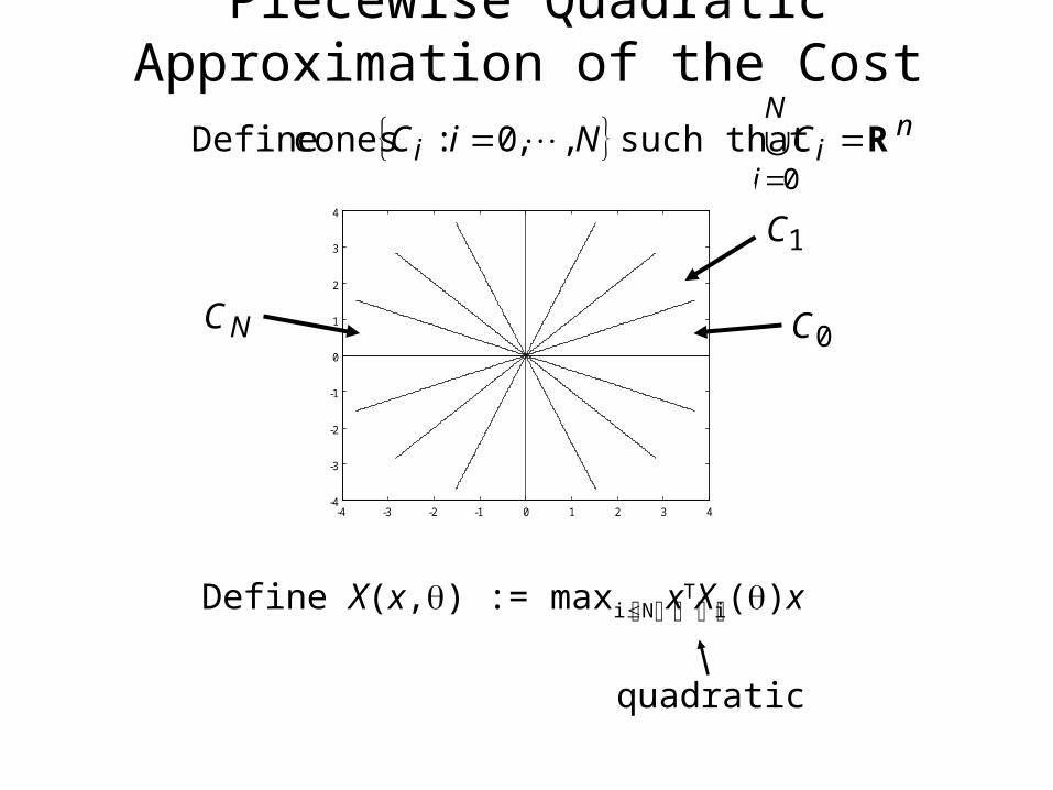
nN
iii CNiC R
0such that ,,0: cones Define
-4 -3 -2 -1 0 1 2 3 4-4
-3
-2
-1
0
1
2
3
4
0C
1C
NC
quadratic
Piecewise Quadratic Approximation of the Cost
Define X(x,) := maxiN xTXi()x
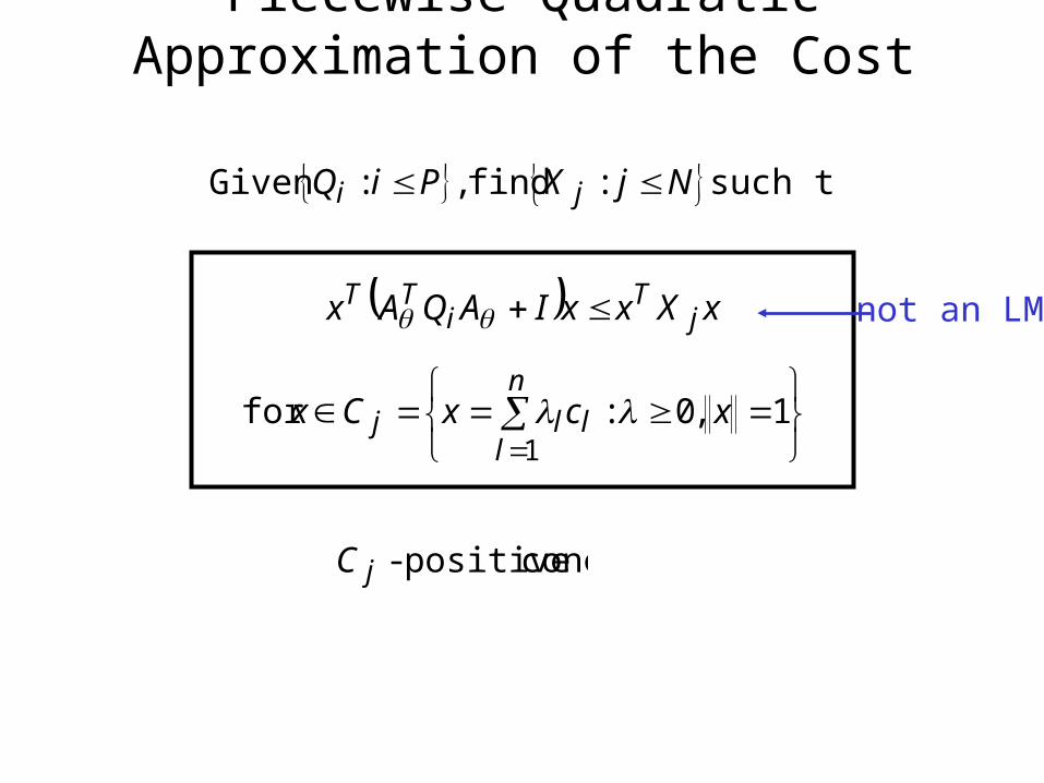
Piecewise Quadratic Approximation of the Cost
xXxxIAQAx jT
iTT
such that : find ,:Given NjXPiQ ji
1,0:for 1
xcxCxn
lllj
cone positive - jC
not an LMI
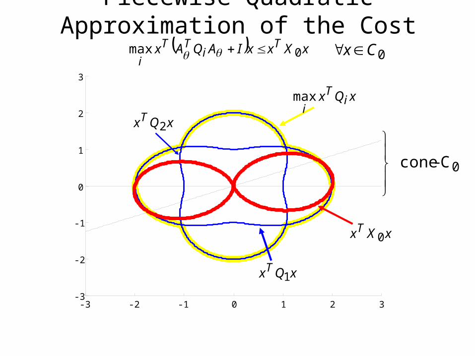
-3 -2 -1 0 1 2 3-3
-2
-1
0
1
2
3
xQxT1
xXxxIAQAx Ti
TT
i0max 0Cx
0C-cone
xQx iT
imax
xXxT0
xQxT2
Piecewise Quadratic Approximation of the Cost
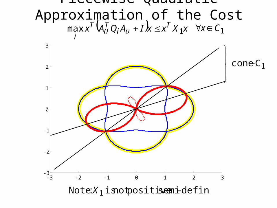
definite-semi positivenot is :Note 1X
1C - cone
Piecewise Quadratic Approximation of the Cost
-3 -2 -1 0 1 2 3-3
-2
-1
0
1
2
3
xXxxIAQAx Ti
TT
i1max 1Cx
-1 -0.8 -0.6 -0.4 -0.2 0 0.2 0.4 0.6 0.8 1-1
-0.8
-0.6
-0.4
-0.2
0
0.2
0.4
0.6
0.8
1
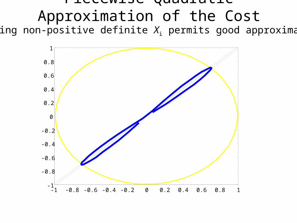
Piecewise Quadratic Approximation of the Cost
Allowing non-positive definite Xi permits good approximation.
-2.5 -2 -1.5 -1 -0.5 0 0.5 1 1.5 2 2.5-2.5
-2
-1.5
-1
-0.5
0
0.5
1
1.5
2
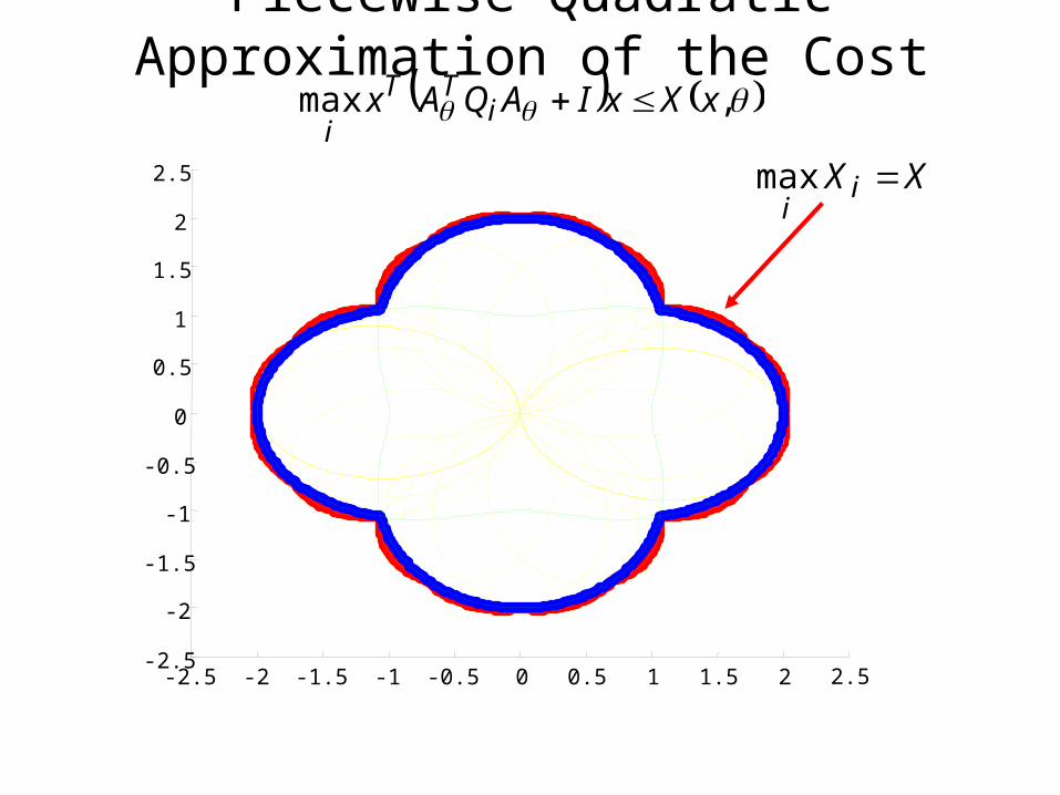
2.5 XX ii
max
,max xXxIAQAx iTT
i
Piecewise Quadratic Approximation of the Cost
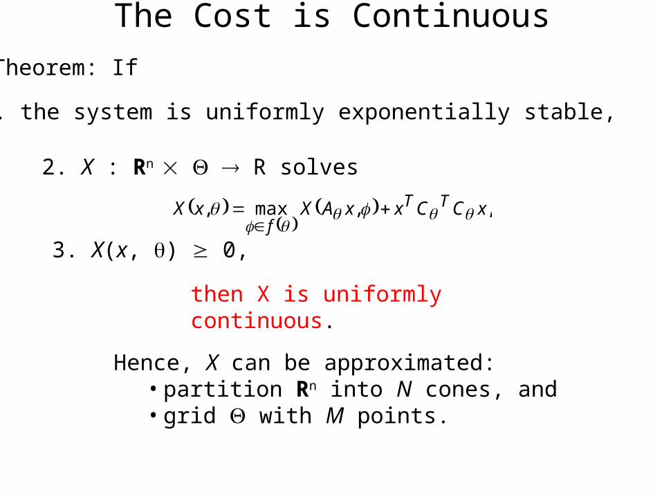
,,max, xCCxxAXxX TT
f
Theorem: If
1. the system is uniformly exponentially stable,
2. X : Rn R solves
3. X(x, ) 0,
then X is uniformly continuous.
Hence, X can be approximated:• partition Rn into N cones, and• grid with M points.
The Cost is Continuous
such that
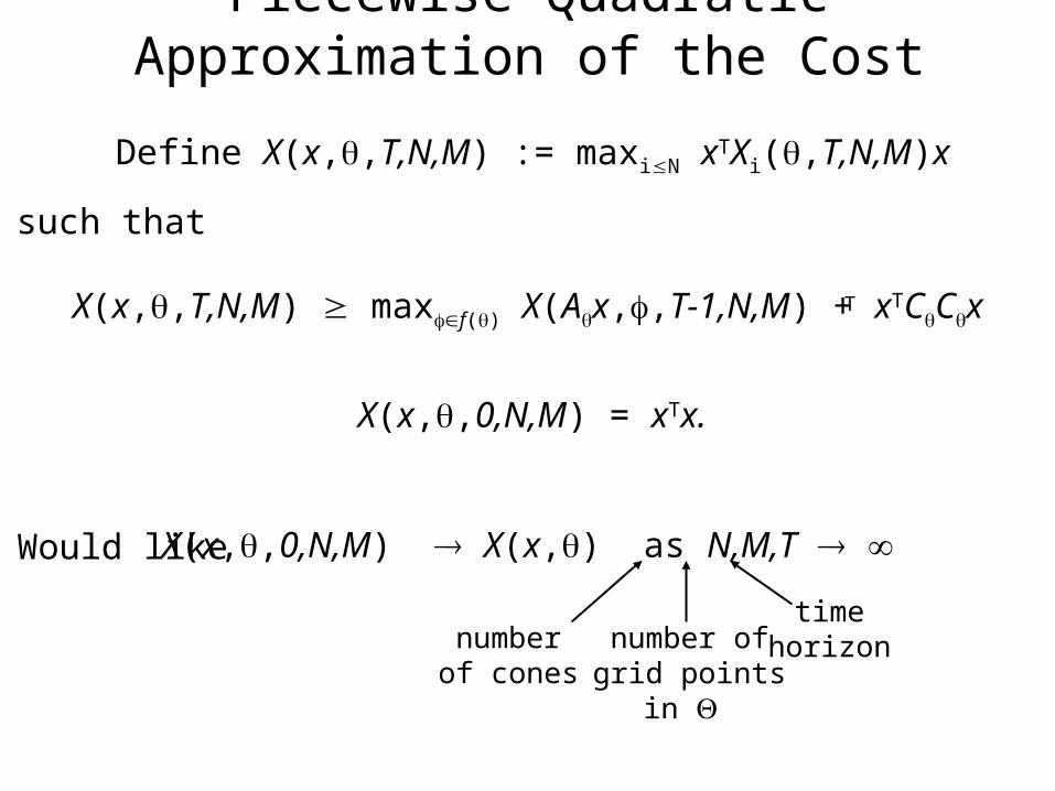
numberof cones
number ofgrid points
in
timehorizon
Piecewise Quadratic Approximation of the Cost
Define X(x,,T,N,M) := maxiN xTXi(,T,N,M)x
X(x,,T,N,M) maxf() X(Ax,,T-1,N,M) + xTCCxT
X(x,,0,N,M) = xTx.
X(x,,0,N,M) X(x,) as N,M,T Would like
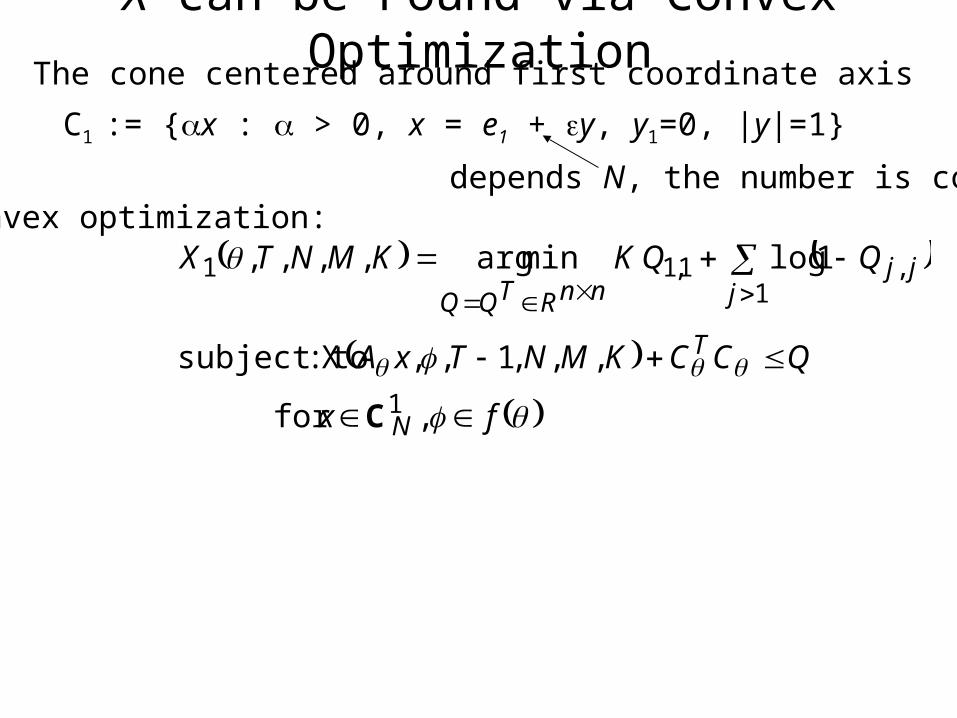
The cone centered around first coordinate axis
fx
QCCKMNTxA
QQKKMNTX
N
T
jjj
nnRTQQ
,for
,,,1,,X:subject to
1logminarg,,,,
1
1,1,11
C
convex optimization:
X can be Found via Convex Optimization
C1 := {x : > 0, x = e1 + y, y1=0, |y|=1}
depends N, the number is cones
The cone centered around first coordinate axis
fx
QCCKMNTxA
QQKKMNTX
N
T
jjj
nnRTQQ
,for
,,,1,,X:subject to
1logminarg,,,,
1
1,1,11
C
convex optimization:
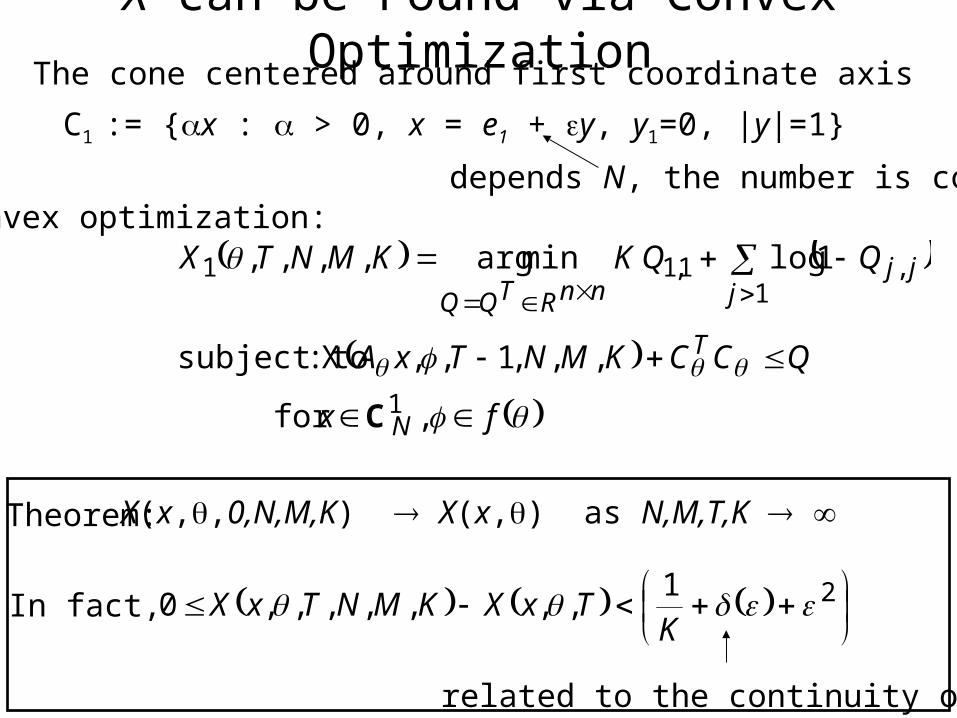
X can be Found via Convex Optimization
C1 := {x : > 0, x = e1 + y, y1=0, |y|=1}
depends N, the number is cones
21
,,,,,,,0 K
TxXKMNTxX
Theorem: X(x,,0,N,M,K) X(x,) as N,M,T,K
related to the continuity of X
In fact,
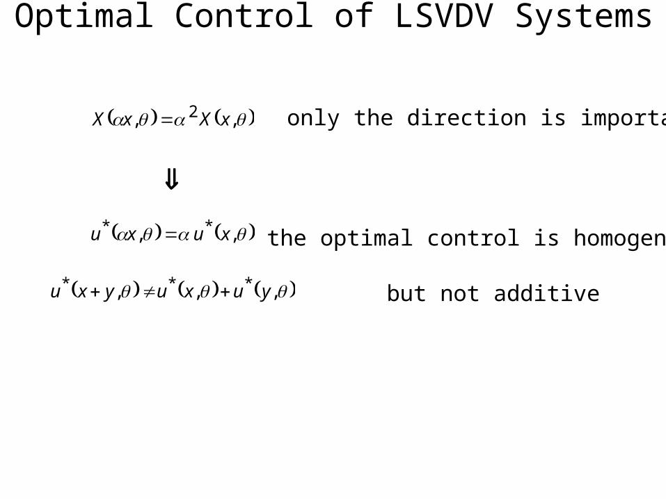
,, 2 xXxX
,, ** xuxu the optimal control is homogeneous
,,, *** yuxuyxu but not additive
only the direction is important
Optimal Control of LSVDV Systems
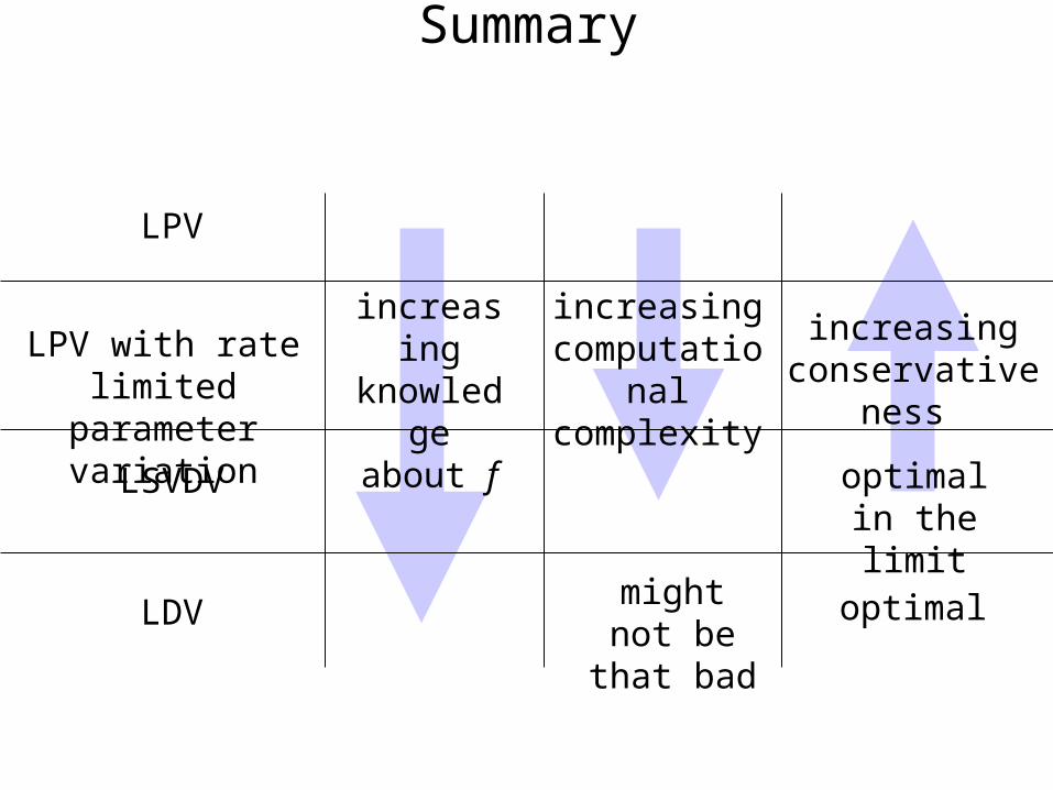
Summary
LPV
LPV with rate limited parameter variation
LSVDV
LDV
increasing knowledge
about f
increasing computational
complexity
increasing conservativeness
optimal in the limit
optimalmight not be that bad