3-DOF Longitudinal Flight Simulation Modeling and Design Using MA

Ryerson UniversityDigital Commons @ Ryerson

Theses and dissertations

1-1-2012

3-DOF Longitudinal Flight Simulation ModelingAnd Design Using MATLAB/SIMULINKUmair AhmedRyerson University

Follow this and additional works at: http://digitalcommons.ryerson.ca/dissertationsPart of the Aerospace Engineering Commons

This Thesis is brought to you for free and open access by Digital Commons @ Ryerson. It has been accepted for inclusion in Theses and dissertations byan authorized administrator of Digital Commons @ Ryerson. For more information, please contact [email protected].

Recommended CitationAhmed, Umair, "3-DOF Longitudinal Flight Simulation Modeling And Design Using MATLAB/SIMULINK" (2012). Theses anddissertations. Paper 1219.

http://digitalcommons.ryerson.ca?utm_source=digitalcommons.ryerson.ca%2Fdissertations%2F1219&utm_medium=PDF&utm_campaign=PDFCoverPages

http://digitalcommons.ryerson.ca/dissertations?utm_source=digitalcommons.ryerson.ca%2Fdissertations%2F1219&utm_medium=PDF&utm_campaign=PDFCoverPages

http://digitalcommons.ryerson.ca/dissertations?utm_source=digitalcommons.ryerson.ca%2Fdissertations%2F1219&utm_medium=PDF&utm_campaign=PDFCoverPages

http://network.bepress.com/hgg/discipline/218?utm_source=digitalcommons.ryerson.ca%2Fdissertations%2F1219&utm_medium=PDF&utm_campaign=PDFCoverPages

http://digitalcommons.ryerson.ca/dissertations/1219?utm_source=digitalcommons.ryerson.ca%2Fdissertations%2F1219&utm_medium=PDF&utm_campaign=PDFCoverPages

mailto:[email protected]

3-DOF LONGITUDINAL FLIGHT SIMULATION MODELING AND DESIGN

USING MATLAB/SIMULINK

By

Umair Ahmed, B. Eng

Mechanical Engineering

Concordia University, 2010

A project presented to the Ryerson University

in partial fulfillment of the degree of

Masters of Engineering

In the program of

Aerospace Engineering

Toronto, Ontario, Canada, 2012

© Umair Ahmed 2012

ii

AUTHOR'S DECLARATION

I hereby declare that I am the sole author of this project report. This is a true copy of

the thesis, including any required final revisions, as accepted by my examiners.

I authorize Ryerson University to lend this project report to other institutions or

individuals for the purpose of scholarly research.

I further authorize Ryerson University to reproduce this project report by

photocopying or by other means, in total or in part, at the request of other institutions or

individuals for the purpose of scholarly research.

I understand that my project report may be made electronically available to the

public.

iii

ABSTRACT

Flight simulators are widely used in aerospace industry for multiple purposes. This

paper highlights the importance of engineering flight simulators and presents a 3 degrees-of-

freedom longitudinal flight simulation model that can be adopted to simulate aircraft

behaviour for engineering analysis. A brief overview of aircraft design process is presented

with reference to flight simulation procedure. A special emphasis is placed on Massachusetts

Institute of Technology's Athena Vortex Lattice program that can be used to calculate

aerodynamic characteristics for a given geometric configuration. The paper explains

modeling of aerodynamics and thrust blocks and shows how they can be linked with

equations of motion block to build a comprehensive flight simulation model. Matlab script

that linearizes and trims equations of motion is also discussed and key stability results are

explained in detail. Simulation test cases are also presented. Several recommendations are

made at the end of the paper on the potential use of simulators and also on ways of

improving the simulation model.

iv

ACKNOWLEDGEMENTS

The author takes this opportunity to gratefully acknowledge the support and advice

of all who have made this project possible.

I am deeply grateful to my supervisor, Dr. Hekmat Alighanbari, whose guidance and

mentorship proved to be invaluable. He is truly a brilliant, extraordinary and an inspiring

professor.

I would like to thank Dr. Jefferey Yokota and Dr. Puren Ouyang for being on my

examination committee. Their presence was a great honour for me.

I would also like to thank Ms. Leah Rogan for her continuous guidance and support

during my master’s degree and in completion of this project. She is very dedicated to her

work with helping students to advance in their studies.

I thank my parents and wife who have been very supportive throughout my

education.

v

Dedicated to my loving parents, wife and son

vi

TABLE OF CONTENTS

1. INTRODUCTION .................................................................................................................... 1

1.1. BACKGROUND AND SIGNIFICANCE .............................................................................. 1

1.2. AIM ............................................................................................................................... 1

1.3. END RESULTS ................................................................................................................ 1

1.4. APPROACH .................................................................................................................... 2

2. ENGINEERING FLIGHT SIMULATION METHODOLOGY ......................................................... 2

2.1. DEFINING AIRCRAFT MASS AND GEOMETRY ............................................................... 3

2.2. DETERMINING AIRCRAFT AERODYNAMIC CHARACTERISTICS ..................................... 3

2.2.1. ANALYTICAL PREDICTION ...................................................................................... 4

2.2.2. WIND TUNNEL TESTING ........................................................................................ 4

2.2.3. FLIGHT TESTING .................................................................................................... 4

2.2.4. AERODYNAMIC DATA CALCULATION USING AVL SOFTWARE .............................. 4

3. BUILDING A FLIGHT SIMULATION MODEL IN SIMULINK ..................................................... 6

3.1. EQUATIONS OF MOTION MODEL BLOCK ..................................................................... 7

3.2. AERODYNAMICS MODEL BLOCK .................................................................................. 8

3.2.1. Wing-Body Block ................................................................................................. 11

3.2.2. Tailplane Block .................................................................................................... 12

3.2.3. CG Location Moment Block ................................................................................ 14

3.2.4. Wind-to-Body Block ............................................................................................ 15

3.3. THRUST BLOCK ........................................................................................................... 17

4. RUNNING THE FLIGHT SIMULATION MODEL IN MATLAB/SIMULINK ................................ 18

4.1. SIMULATION INITIALIZATION SCRIPT ......................................................................... 18

4.2. TRIMMING AND LINEARIZATION SCRIPT.................................................................... 20

5. VERIFICATION OF THE FLIGHT SIMULATION MODEL RESULTS ......................................... 21

TRIMMED INPUTS .................................................................................................................. 23

vii

STATIC STABILITY ................................................................................................................... 23

LINEARIZED LONGITUDINAL EQUATIONS OF MOTION ......................................................... 23

DYNAMIC STABILITY .............................................................................................................. 25

HORIZONTAL TAIL-VOLUME RATIO VH ................................................................................. 26

SIMULATION CASES ................................................................................................................... 27

VARIATION IN WING QUARTER CHORD ........................................................................... 27

VARIATION IN THRUST ....................................................................................................... 27

VARIATION IN WING AREA Sref ......................................................................................... 28

VARIATION IN HORIZONTAL TAIL AREA St ......................................................................... 29

VARIATION IN MACH NUMBER ......................................................................................... 29

6. CONCLUSION AND RECOMMENDATIONS ......................................................................... 30

REFERENCES .............................................................................................................................. 33

APPENDIX A: SIMULATION INITIALIZATION SCRIPT ................................................................. 34

APPENDIX B: TRIMMING AND LINEARIZATION SCRIPT ............................................................. 36

APPENDIX C: AVL GEOMETRIC INPUT FILE FOR DATA CALCULATION ..................................... 39

APPENDIX D: SAMPLE AERODYNAMIC DATA GENERATED BY AVL ........................................... 42

APPENDIX E ............................................................................................................................... 43

viii

LIST OF FIGURES

Figure 1: Aerodynamic Geometry in AVL showing Wing and Horizontal Stabilizer ................... 5

Figure 2: Top Level Flight Simulation Model .............................................................................. 7

Figure 3: Equations of Motion Block ........................................................................................... 8

Figure 4: Top Level Aerodynamics Block .................................................................................... 9

Figure 5: Aerodynamics Block Sub-system ............................................................................... 10

Figure 6: Wing-body Aerodynamics Block ................................................................................ 11

Figure 7: Look-up Table Block for storing wing aerodynamic data .......................................... 11

Figure 8: Sample Look-up Table storing lift coefficient CL for various Alpha for Mach of 0.22 12

Figure 9: Tailplane Block ........................................................................................................... 12

Figure 10: Tailplane Block Sub-system ...................................................................................... 13

Figure 11: Tailplane At Quarter Chord Block ............................................................................ 13

Figure 12: Tailplane At Quarter Chord Block Sub-system with Functions for tail aero

coefficients ................................................................................................................................ 14

Figure 13: CG Moment Block with its Sub-System ................................................................... 15

Figure 14: Wind to Body Block .................................................................................................. 15

Figure 15: Wind to Body Block Sub-system .............................................................................. 16

Figure 16: The function block calculating Xaerob ..................................................................... 16

Figure 17: Thrust Block ............................................................................................................. 17

Figure 18: Thrust Block Sub-system .......................................................................................... 18

Figure 19: A Complete Simulation Model Sketch ..................................................................... 43

ix

LIST OF SYMBOLS

Abbreviations

AoA angle of attack

AVL Athena Vortex Lattice

CFD Computational Fluid Dynamics

CG Center of Gravity

DATCOM Data Compendium (US Air Force)

DoF Degree-of-Freedom

FAR Federal Aviation Regulation

GNU General Public License

Hstab Horizontal Stabilizer

LTI Linear Time Invariant

MIT Massachusetts Institute of Technology

STOL Short Take-off and Landing

Parameters

alpha_wb wing body angle of attack

bt tail span

wing mean aerodynamic chord

Cmα pitching moment curve with respect to angle of attack

CLwb wing body lift coefficient

CDwb wing body drag coefficient

Cmwb wing body pitching moment coefficient

CLT total tail lift coefficient

CDT total tail drag coefficient

CLTail tail lift coefficient

CDTail tail drag coefficient

CMtail tail pitching moment coefficient

Iyy moment of inertia

M Mach number

Maerob pitching moment in the body axis

x

Mw pitching moment in the wind axis

lt distance between CG and horizontal tail quarter chord

q pitch rate

Q dynamic pressure

Sref wing reference area

St horizontal tail area

u forward velocity

V velocity

w vertical velocity

W weight

xwb x-distance between CG and wing quarter chord

Xaerob x-force in the body axis

Xw x-force in the wind axis

Zaerob z-force in the body axis

Zw z-force in the wind axis

Greek Letters

α angle of attack

ε downwash

1

1. INTRODUCTION

1.1. BACKGROUND AND SIGNIFICANCE

Since the advent of engineering, simulation of physical systems has been regarded as

great means to understand and predict system's behaviour. Aircraft modeling and simulation

is no exception and the use of flight simulators dates back to the early phase of aviation

industry. The simulators were primarily designed for pilot training purposes but soon the

benefits of flight simulation to support engineering designs were realized and flight

simulators started to play an important role in aircraft design. The engineering flight

simulators reduce lifecycle costs because development and testing of complex aircraft

systems can be done before actual flight tests. The simulator provides useful data that can be

used to assess performance and behaviour of the aircraft and its systems. Moreover, the

response of aircraft systems can be visualized in various platforms. There are different

objectives of the engineering simulation study in flight simulators. A simulation model may

be built to analyze performance, stability characteristics and mission of a flight vehicle.

1.2. AIM

The aim of this project is to build a 3 degrees-of-freedom longitudinal flight

simulation model in Simulink to allow rapid configuration and flight dynamic analysis of an

aircraft. The model will have a capability to solve longitudinal equations of motion for any

given aircraft geometry. Furthermore, the equations will be trimmed to obtain the

longitudinal equations of motion consisting of aerodynamic stability and control derivatives

which helps in determining the longitudinal dynamic stability characteristics of an aircraft.

The simulation model will provide results to determine whether an aircraft is statically and

dynamically stable longitudinally and can be trimmed at reference flight condition.

1.3. END RESULTS

The flight simulation model offers many benefits for a new aircraft development

projects. It can assist an aircraft designer in meeting Federal Aviation Regulations (FARs)

related to aircraft manoeuvring and handling qualities. The designer is able to predict aircraft

2

behaviour in specific flight conditions and can produce a stable and controllable aircraft by

determining its stability characteristics. The simulation-based testing will save time and effort

prior to conducting actual flight tests. The simulation model can also be extended to serve

any purpose of study. Most importantly, the simulation model can be used in academics to

learn and teach the subject of flight dynamics.

1.4. APPROACH

The project will be initiated by developing a simulation structure for a 3-DoF

longitudinal model in Simulink. The simulation model will consist of aerodynamics, thrust,

and equations of motion blocks. The aerodynamics block will contain various sub-systems

and aerodynamic data for a generic STOL aircraft. The aerodynamic data will be calculated

using Massachusetts Institute of Technology’s (MIT) Athena Vortex Lattice (AVL) open source

software AVL and will be stored in the look-up tables. Once the model is solved in Simulink, a

linearization script written in Matlab will be used to trim and linearize the model. The

resulting model in linear state-space format will be used to obtain longitudinal response in

order to determine the dynamic stability characteristics of an aircraft.

2. ENGINEERING FLIGHT SIMULATION METHODOLOGY

Aircraft flight simulation is a part of overall aircraft design process and is complex,

time consuming and iterative in nature. The process involves various technical steps and

requires use of sophisticated software having modeling and simulation capabilities such as

Matlab/Simulink. It is pertinent to highlight key aircraft design steps related to flight

simulation as follows [1]:

I. Defining Aircraft Mass and Geometry

II. Determining Aircraft Aerodynamic Characteristics

III. Creating Aircraft Flight Simulation

IV. Designing Flight Control Laws

V. Completing the Design Process

For this project, only the first three steps are followed as the last two steps are

beyond the scope.

3

2.1. DEFINING AIRCRAFT MASS AND GEOMETRY

It is the intent of this project to render the flight simulation model open source so

that it is compatible with an aircraft of any geometry and respective data. This is ensured by

constructing an aerodynamic model that is comprehensive to intake aerodynamic data based

on any geometry. In other words, to perform simulation for a different aircraft, its respective

data can be incorporated in the model and equations of motions can be solved. It is

important to discuss the procedure to be followed for a new aircraft geometric configuration.

The process starts from establishing the system level requirements and specification for a

new aircraft which results in performance criteria of an aircraft. The aircraft geometry is

determined at this stage to calculate stability and control derivatives that directly affects

aircraft performance.

For this project, the mass and geometry data for a generic short take-off and landing

STOL transport aircraft is used [2]. The mass properties data include aircraft weight, center of

gravity location CG and moment of inertia Iyy. The geometric data includes wing reference

area Sref, horizontal tail area St, distance between CG and horizontal tail quarter chord lt, tail

span bt, wing mean aerodynamic chord and x-distance between CG and wing quarter chord

xwb. All the data is stored in the Initialization script (appendix A).

2.2. DETERMINING AIRCRAFT AERODYNAMIC CHARACTERISTICS

Determining the aerodynamic characteristics of an aircraft is one of the crucial steps

of the modeling and simulation study. The equations of motion can only be solved once the

aerodynamic forces and moments acting on the aircraft body are found. Before the

aerodynamic forces and moments can be calculated, the aerodynamics coefficients for both

wing and tail are required.

There exist three methods to obtain aerodynamic characteristics for a given

geometric configuration namely analytical prediction, wind tunnel testing and flight testing.

Each method is briefly explained below and the chosen method for the project is discussed at

the end of this section.

4

2.2.1. ANALYTICAL PREDICTION

Calculating aerodynamic data for an aircraft analytically is a quick and less-expensive

method. Computational Fluid Dynamics (CFD) analysis is a modern method that is rigorous

and broad. However, to quickly gain an insight into the aerodynamic behaviour of an aircraft,

a very useful analytical prediction method called USAF Digital Datcom program can be used

to determine aerodynamic characteristics. A Digital Datcom input file defines the geometric

configuration of the aircraft and the flight conditions to calculate the aerodynamic

coefficients [3]. However, Datcom is not open source and needs to be purchased.

Fortunately, there exists alternative software developed by Massachusetts Institute of

Technology called AVL [4]. AVL is an open source software that can be used to quickly predict

aerodynamics characteristics for a given aircraft geometric configuration. However, an input

file of aircraft geometry is needed and is not easy to create one for a given aircraft.

2.2.2. WIND TUNNEL TESTING

To perform wind tunnel testing, a scaled model or full-sized prototype is needed

which makes the method expensive and time consuming. The method is used mainly by

aircraft manufacturers on new development projects.

2.2.3. FLIGHT TESTING

Flight testing is another expensive and time-consuming process and cannot be used in

the very early stages of design since the aircraft is yet to be built.

2.2.4. AERODYNAMIC DATA CALCULATION USING AVL SOFTWARE

It is obvious based on the previous discussion that the last two methods cannot be

adopted in the academic setting and the ideal method for learning purposes should the

utilization of either the digital Datcom program or AVL. Since AVL is open source and

released under the GNU General Public License, it is the only method used for this project.

However, there are limitations as discussed later.

To use AVL, a configuration definition for an aircraft is required in the form of

keyword-driven geometry input file. This input file consists of defined sections and also uses

another input airfoil file for a particular aircraft wing to generate the aerodynamic data [4].

AVL offers several input files for selected aircrafts; however, generating an input file

5

manually for any other aircraft is complex and requires an extensive geometric data. Since

only the wing and horizontal stabilizer aerodynamics is to be simulated in this project, a

simple input file can be generated for a given STOL aircraft as both the wing and horizontal

stabilizer geometric data is available. However, a complete shape or drawing is not available

and some serious limitations should be kept in mind. The key geometric parameters are

defined for both the wing and stab. As the airfoil data for this particular aircraft is not known,

a Boeing 737-800 airfoil data is used. This introduces inaccuracy in the aerodynamic

coefficients calculated. However, this is the only method available to generate aerodynamic

data for an aircraft for which the much needed mass properties and key geometric

parameters are known with the exception of thrust data. The compromise made at this stage

is bound to have a significant impact on simulation results. The geometric input file for the

STOL aircraft is shown in appendix C. The generated data at a sample angle of attack is shown

in appendix D.

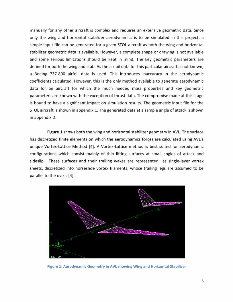
Figure 1 shows both the wing and horizontal stabilizer geometry in AVL. The surface

has discretized finite elements on which the aerodynamics forces are calculated using AVL's

unique Vortex-Lattice Method [4]. A Vortex-Lattice method is best suited for aerodynamic

configurations which consist mainly of thin lifting surfaces at small angles of attack and

sideslip. These surfaces and their trailing wakes are represented as single-layer vortex

sheets, discretized into horseshoe vortex filaments, whose trailing legs are assumed to be

parallel to the x-axis [4].

Figure 1: Aerodynamic Geometry in AVL showing Wing and Horizontal Stabilizer

6

The aerodynamic data for both the wing and horizontal stabilizer is stored in Simulink

look-up tables. The data include the lift, drag and pitching moment coefficients for the wing

and total lift and drag coefficients for the horizontal stabilizer.

3. BUILDING A FLIGHT SIMULATION MODEL IN SIMULINK

The objective of the flight simulation model is to determine whether a given aircraft is

longitudinally stable and can be trimmed at a chosen flight condition. Therefore, it is

essential to model the aircraft components that have a significant impact on the static and

dynamic stability of an aircraft. Stability is the tendency of an aircraft to converge on the

initial equilibrium condition following a small disturbance from trim [5]. To establish trim

equilibrium, a horizontal stabiliser (Hstab) angle and thrust is adjusted to obtain a lift force

sufficient to support the weight and a thrust force to balance the drag at the desired speed.

The trim adjustment is therefore an important result to be achieved through the simulation

model. The model deals with the longitudinal trim only. Another essential task is to

determine the dynamic stability of a given aircraft. This requires solution of the longitudinal

equations of motion and finding both dynamic stability modes, the short period pitching

oscillation and the phugoid. The equations of motion can be solved by trimming the

simulation model and a dynamic response can be obtained.

The simulation model is designed in the graphical environment of Simulink in

conjunction with Matlab [6]. Simulink is the preferred choice since the model can easily be

visualized. The model consists of three main blocks namely Equations of Motion,

Aerodynamics and Thrust blocks. Each block is defined by an input and an output. The

functionality of each block is implemented using flight dynamics theory. All the blocks are

then linked to build a flight simulation model that can be run to observe aircraft behaviour.

The modelling process starts with the aerodynamics of an aircraft in which both the wing and

tail contributions are modelled. Both models become a subsystem of the aerodynamics

block. The thrust block is then constructed which is linked with the equation of motion block

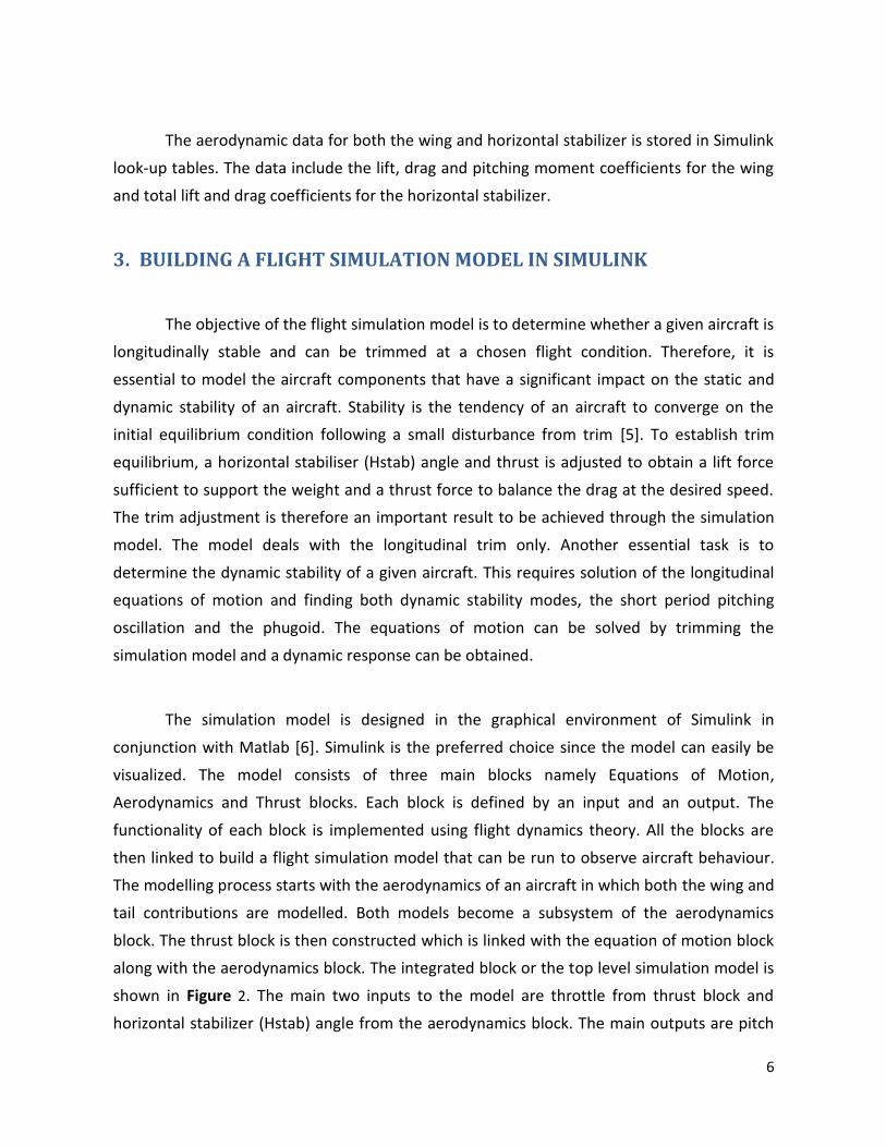
along with the aerodynamics block. The integrated block or the top level simulation model is

shown in Figure 2. The main two inputs to the model are throttle from thrust block and

horizontal stabilizer (Hstab) angle from the aerodynamics block. The main outputs are pitch

7

angle theta, pitch rate q, forward velocity u and vertical velocity w. Each block of the top

level simulation model is explained in the rest of this section.

Figure 2: Top Level Flight Simulation Model

3.1. EQUATIONS OF MOTION MODEL BLOCK

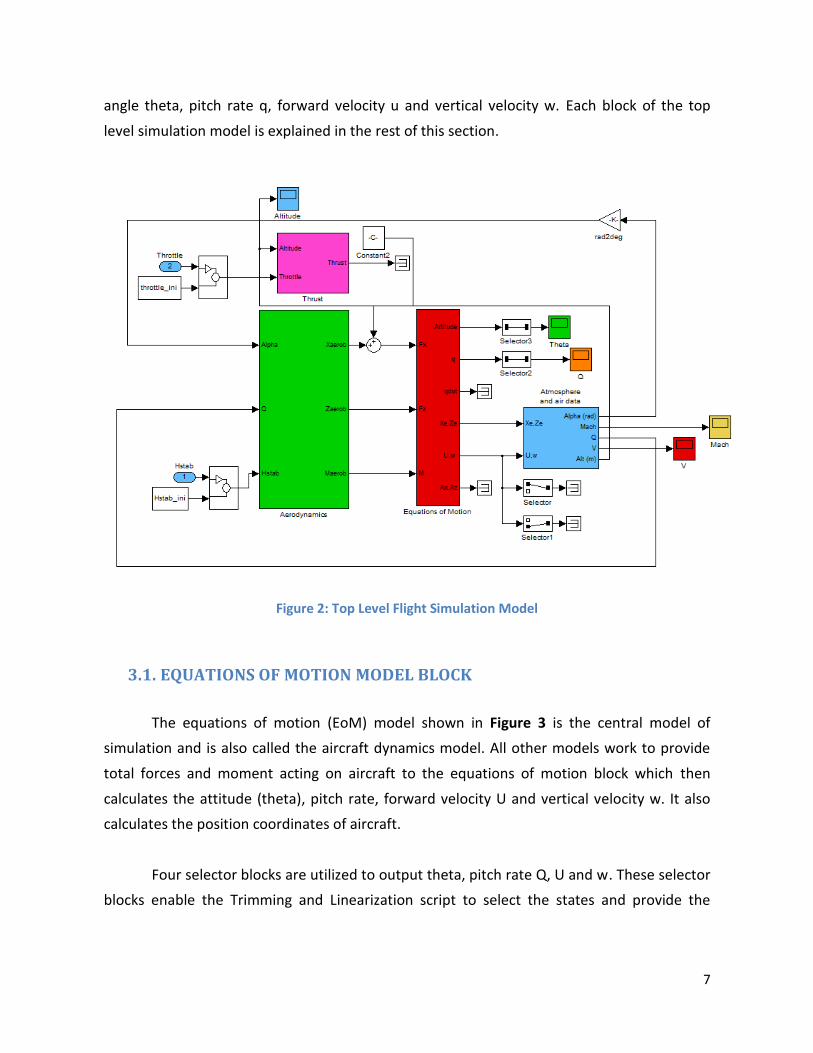
The equations of motion (EoM) model shown in Figure 3 is the central model of

simulation and is also called the aircraft dynamics model. All other models work to provide

total forces and moment acting on aircraft to the equations of motion block which then

calculates the attitude (theta), pitch rate, forward velocity U and vertical velocity w. It also

calculates the position coordinates of aircraft.

Four selector blocks are utilized to output theta, pitch rate Q, U and w. These selector

blocks enable the Trimming and Linearization script to select the states and provide the

8

trimmed input. Moreover, the state-space variables are defined using selectors where the

variables needed are U, w, q and theta.

Another block called Atmosphere and Air Data is constructed to get alpha, Mach

number, dynamics pressure Q, velocity V and altitude from Xe, Ze, U and w. This block is also

useful in creating a closed loop simulation model where alpha, Q, V and altitude are fed back

to the model and help the model find the operating point to linearize the system.

Figure 3: Equations of Motion Block

3.2. AERODYNAMICS MODEL BLOCK

The aerodynamic model can be regarded as the most complex and important model

of the flight simulation model. It solves the aerodynamic forces and moments acting on the

aircraft about its center of gravity. These forces and moments are then used to solve

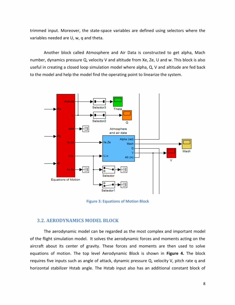
equations of motion. The top level Aerodynamic Block is shown in Figure 4. The block

requires five inputs such as angle of attack, dynamic pressure Q, velocity V, pitch rate q and

horizontal stabilizer Hstab angle. The Hstab input also has an additional constant block of

9

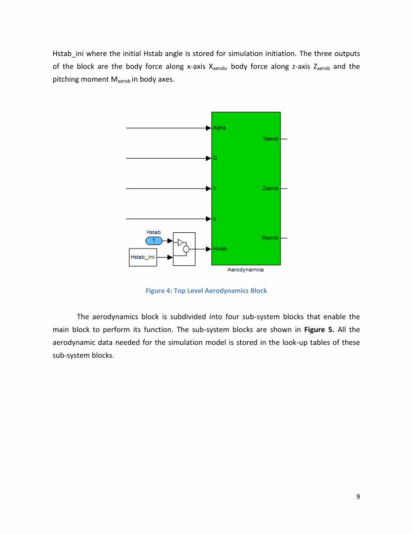
Hstab_ini where the initial Hstab angle is stored for simulation initiation. The three outputs

of the block are the body force along x-axis Xaerob, body force along z-axis Zaerob and the

pitching moment Maerob in body axes.

Figure 4: Top Level Aerodynamics Block

The aerodynamics block is subdivided into four sub-system blocks that enable the

main block to perform its function. The sub-system blocks are shown in Figure 5. All the

aerodynamic data needed for the simulation model is stored in the look-up tables of these

sub-system blocks.

10

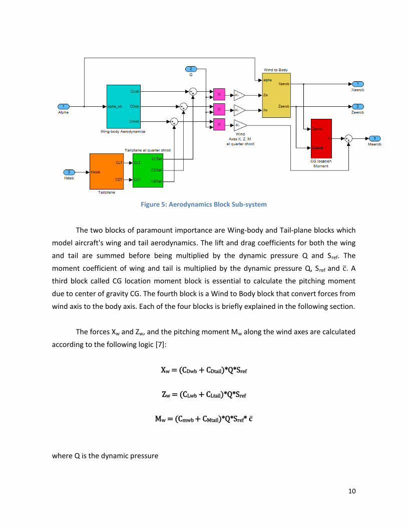
Figure 5: Aerodynamics Block Sub-system

The two blocks of paramount importance are Wing-body and Tail-plane blocks which

model aircraft's wing and tail aerodynamics. The lift and drag coefficients for both the wing

and tail are summed before being multiplied by the dynamic pressure Q and Sref. The

moment coefficient of wing and tail is multiplied by the dynamic pressure Q, Sref and . A

third block called CG location moment block is essential to calculate the pitching moment

due to center of gravity CG. The fourth block is a Wind to Body block that convert forces from

wind axis to the body axis. Each of the four blocks is briefly explained in the following section.

The forces Xw and Zw, and the pitching moment Mw along the wind axes are calculated

according to the following logic [7]:

Xw = (CDwb + CDtail)*Q*Sref

Zw = (CLwb + CLtail)*Q*Sref

Mw = (Cmwb + CMtail)*Q*Sref*

where Q is the dynamic pressure

11

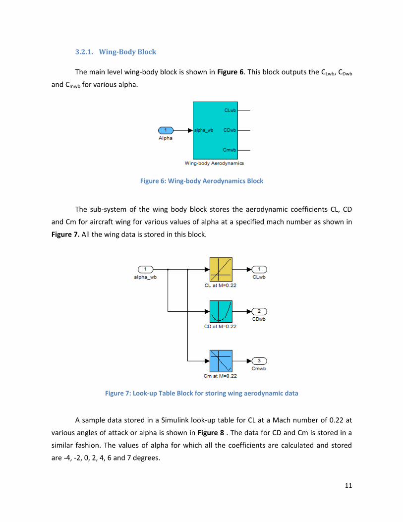
3.2.1. Wing-Body Block

The main level wing-body block is shown in Figure 6. This block outputs the CLwb, CDwb

and Cmwb for various alpha.

Figure 6: Wing-body Aerodynamics Block

The sub-system of the wing body block stores the aerodynamic coefficients CL, CD

and Cm for aircraft wing for various values of alpha at a specified mach number as shown in

Figure 7. All the wing data is stored in this block.

Figure 7: Look-up Table Block for storing wing aerodynamic data

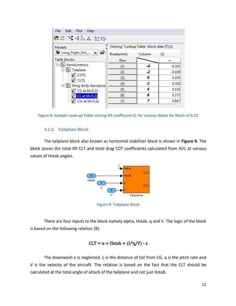
A sample data stored in a Simulink look-up table for CL at a Mach number of 0.22 at

various angles of attack or alpha is shown in Figure 8 . The data for CD and Cm is stored in a

similar fashion. The values of alpha for which all the coefficients are calculated and stored

are -4, -2, 0, 2, 4, 6 and 7 degrees.

12

Figure 8: Sample Look-up Table storing lift coefficient CL for various Alpha for Mach of 0.22

3.2.2. Tailplane Block

The tailplane block also known as horizontal stabilizer block is shown in Figure 9. The

block stores the total lift CLT and total drag CDT coefficients calculated from AVL at various

values of Hstab angles.

Figure 9: Tailplane Block

There are four inputs to the block namely alpha, Hstab, q and V. The logic of the block

is based on the following relation [8]:

CLT = α + Hstab + (lt*q/V) - ε

The downwash ε is neglected. lt is the distance of tail from CG, q is the pitch rate and

V is the velocity of the aircraft. The relation is based on the fact that the CLT should be

calculated at the total angle of attack of the tailplane and not just Hstab.

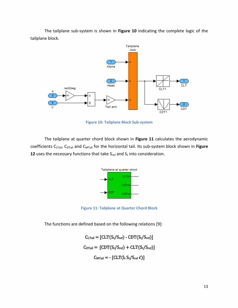
13

The tailplane sub-system is shown in Figure 10 indicating the complete logic of the

tailplane block.

Figure 10: Tailplane Block Sub-system

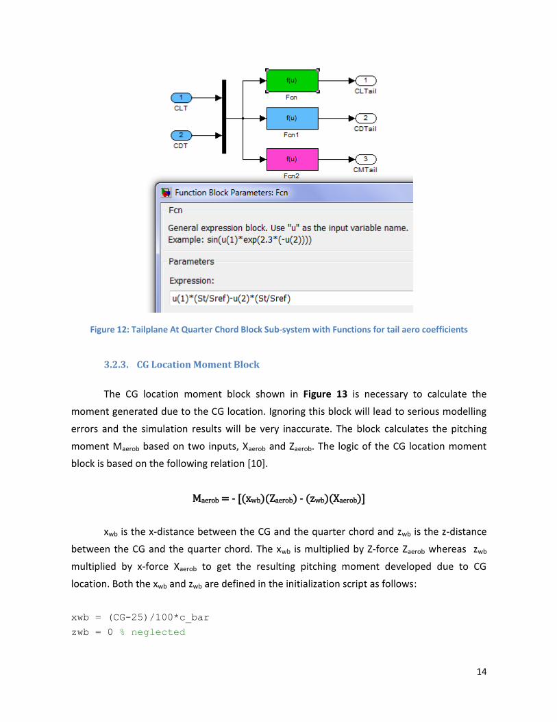
The tailplane at quarter chord block shown in Figure 11 calculates the aerodynamic

coefficients CLTail, CDTail and CMTail for the horizontal tail. Its sub-system block shown in Figure

12 uses the necessary functions that take Sref and St into consideration.

Figure 11: Tailplane at Quarter Chord Block

The functions are defined based on the following relations [9]:

CLTail = [CLT(St/Sref) - CDT(St/Sref)]

CDTail = [CDT(St/Sref) + CLT(St/Sref)]

CMTail = - [CLT(lt St/Sref )]

14

Figure 12: Tailplane At Quarter Chord Block Sub-system with Functions for tail aero coefficients

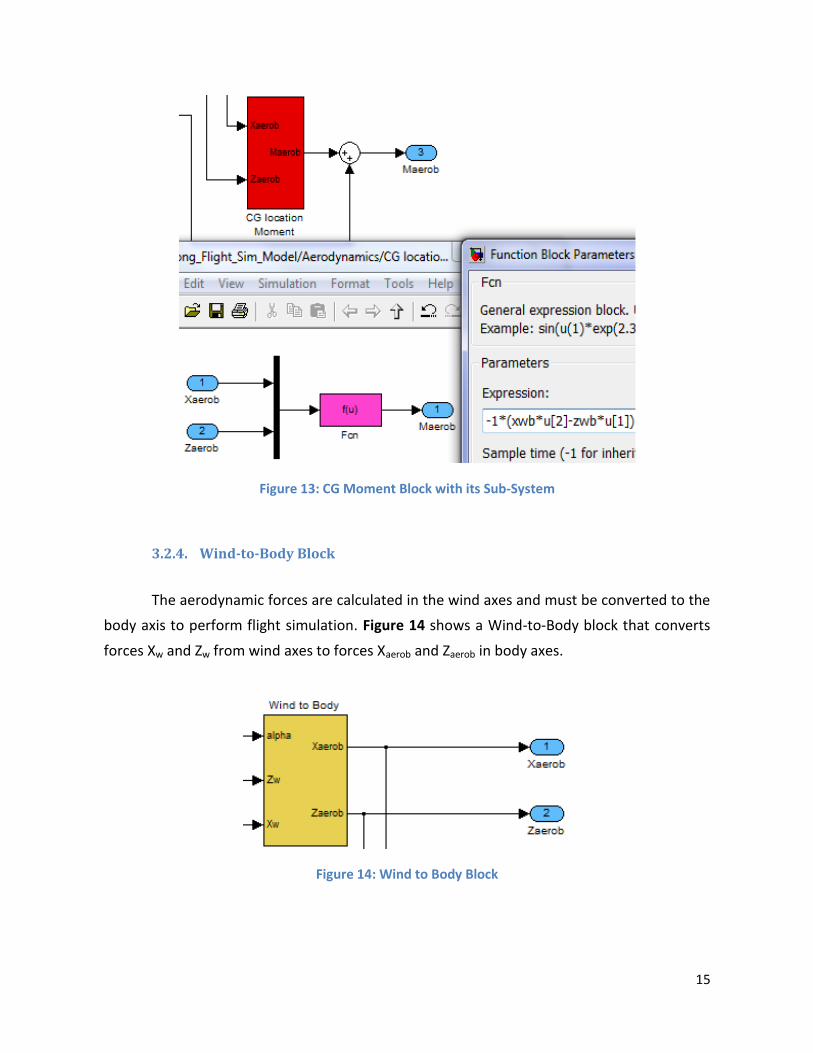
3.2.3. CG Location Moment Block

The CG location moment block shown in Figure 13 is necessary to calculate the

moment generated due to the CG location. Ignoring this block will lead to serious modelling

errors and the simulation results will be very inaccurate. The block calculates the pitching

moment Maerob based on two inputs, Xaerob and Zaerob. The logic of the CG location moment

block is based on the following relation [10].

Maerob = - [(xwb)(Zaerob) - (zwb)(Xaerob)]

xwb is the x-distance between the CG and the quarter chord and zwb is the z-distance

between the CG and the quarter chord. The xwb is multiplied by Z-force Zaerob whereas zwb

multiplied by x-force Xaerob to get the resulting pitching moment developed due to CG

location. Both the xwb and zwb are defined in the initialization script as follows:

xwb = (CG-25)/100*c_bar

zwb = 0 % neglected

15

Figure 13: CG Moment Block with its Sub-System

3.2.4. Wind-to-Body Block

The aerodynamic forces are calculated in the wind axes and must be converted to the

body axis to perform flight simulation. Figure 14 shows a Wind-to-Body block that converts

forces Xw and Zw from wind axes to forces Xaerob and Zaerob in body axes.

Figure 14: Wind to Body Block

16

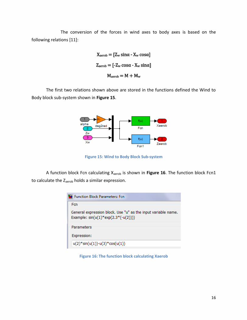
The conversion of the forces in wind axes to body axes is based on the

following relations [11]:

Xaerob = [Zw sinα - Xw cosα]

Zaerob = [-Zw cosα - Xw sinα]

Maerob = M + Mw

The first two relations shown above are stored in the functions defined the Wind to

Body block sub-system shown in Figure 15.

Figure 15: Wind to Body Block Sub-system

A function block Fcn calculating Xaerob is shown in Figure 16. The function block Fcn1

to calculate the Zaerob holds a similar expression.

Figure 16: The function block calculating Xaerob

17

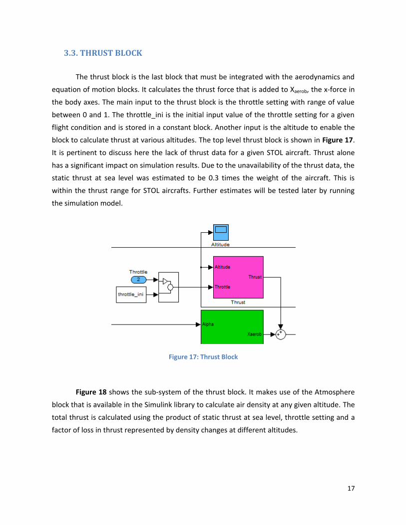
3.3. THRUST BLOCK

The thrust block is the last block that must be integrated with the aerodynamics and

equation of motion blocks. It calculates the thrust force that is added to Xaerob, the x-force in

the body axes. The main input to the thrust block is the throttle setting with range of value

between 0 and 1. The throttle_ini is the initial input value of the throttle setting for a given

flight condition and is stored in a constant block. Another input is the altitude to enable the

block to calculate thrust at various altitudes. The top level thrust block is shown in Figure 17.

It is pertinent to discuss here the lack of thrust data for a given STOL aircraft. Thrust alone

has a significant impact on simulation results. Due to the unavailability of the thrust data, the

static thrust at sea level was estimated to be 0.3 times the weight of the aircraft. This is

within the thrust range for STOL aircrafts. Further estimates will be tested later by running

the simulation model.

Figure 17: Thrust Block

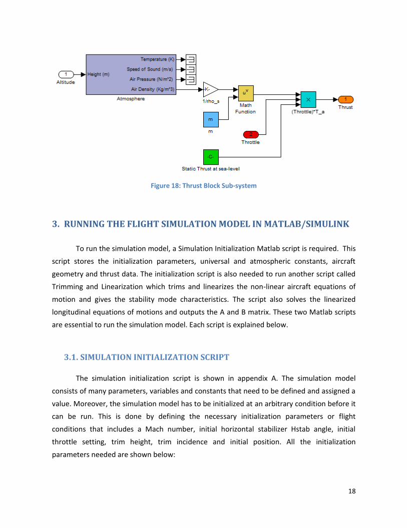
Figure 18 shows the sub-system of the thrust block. It makes use of the Atmosphere

block that is available in the Simulink library to calculate air density at any given altitude. The

total thrust is calculated using the product of static thrust at sea level, throttle setting and a

factor of loss in thrust represented by density changes at different altitudes.

18

Figure 18: Thrust Block Sub-system

3. RUNNING THE FLIGHT SIMULATION MODEL IN MATLAB/SIMULINK

To run the simulation model, a Simulation Initialization Matlab script is required. This

script stores the initialization parameters, universal and atmospheric constants, aircraft

geometry and thrust data. The initialization script is also needed to run another script called

Trimming and Linearization which trims and linearizes the non-linear aircraft equations of

motion and gives the stability mode characteristics. The script also solves the linearized

longitudinal equations of motions and outputs the A and B matrix. These two Matlab scripts

are essential to run the simulation model. Each script is explained below.

3.1. SIMULATION INITIALIZATION SCRIPT

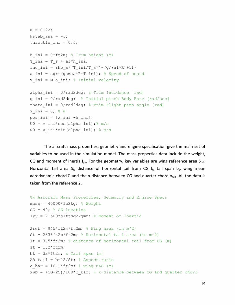
The simulation initialization script is shown in appendix A. The simulation model

consists of many parameters, variables and constants that need to be defined and assigned a

value. Moreover, the simulation model has to be initialized at an arbitrary condition before it

can be run. This is done by defining the necessary initialization parameters or flight

conditions that includes a Mach number, initial horizontal stabilizer Hstab angle, initial

throttle setting, trim height, trim incidence and initial position. All the initialization

parameters needed are shown below:

19

M = 0.22;

Hstab_ini = -3;

throttle_ini = 0.5;

h_ini = 0*ft2m; % Trim height (m)

T_ini = T_s + a1*h_ini;

rho_ini = rho_s*(T_ini/T_s)^-(g/(a1*R)+1);

a_ini = sqrt(gamma*R*T_ini); % Speed of sound

v_ini = M*a_ini; % Initial velocity

alpha_ini = 0/rad2deg; % Trim Incidence [rad]

q_ini = 0/rad2deg; % Initial pitch Body Rate [rad/sec]

theta_ini = 0/rad2deg; % Trim Flight path Angle [rad]

x_ini = 0; % m

pos_ini = [x_ini -h_ini];

U0 = v_ini*cos(alpha_ini);% m/s

w0 = v_ini*sin(alpha_ini); % m/s

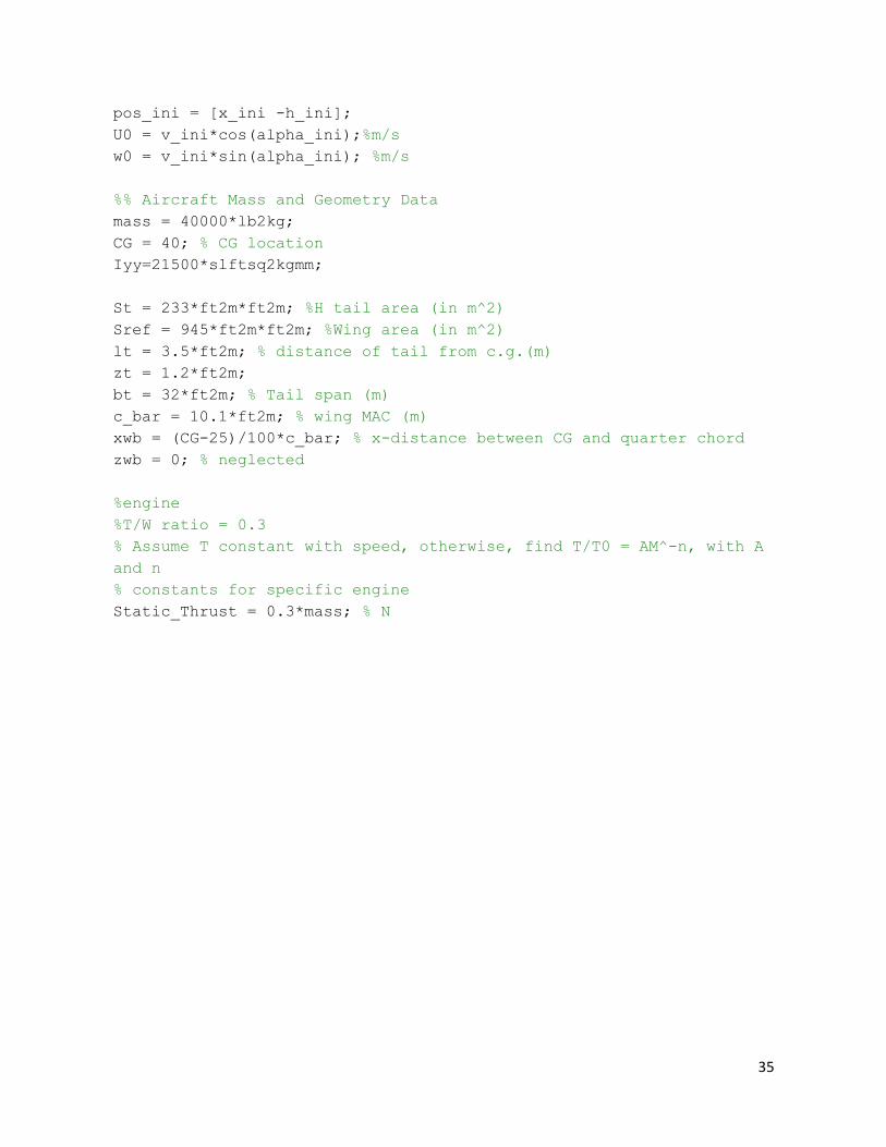
The aircraft mass properties, geometry and engine specification give the main set of

variables to be used in the simulation model. The mass properties data include the weight,

CG and moment of inertia Iyy. For the geometry, key variables are wing reference area Sref,

Horizontal tail area St, distance of horizontal tail from CG lt, tail span bt, wing mean

aerodynamic chord and the x-distance between CG and quarter chord xwb. All the data is

taken from the reference 2.

%% Aircraft Mass Properties, Geometry and Engine Specs

mass = 40000*lb2kg; % Weight

CG = 40; % CG location

Iyy = 21500*slftsq2kgmm; % Moment of Inertia

Sref = 945*ft2m*ft2m; % Wing area (in m^2)

St = 233*ft2m*ft2m; % Horizontal tail area (in m^2)

lt = 3.5*ft2m; % distance of horizontal tail from CG (m)

zt = 1.2*ft2m;

bt = 32*ft2m; % Tail span (m)

AR_tail = bt^2/St; % Aspect ratio

c_bar = 10.1*ft2m; % wing MAC (m)

xwb = (CG-25)/100*c_bar; % x-distance between CG and quarter chord

20

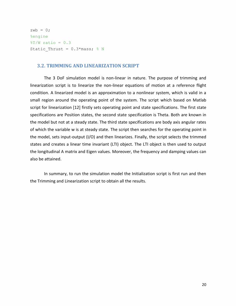
zwb = 0;

%engine

%T/W ratio = 0.3

Static_Thrust = 0.3*mass; % N

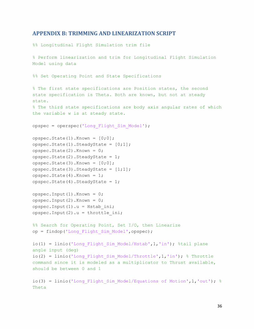
3.2. TRIMMING AND LINEARIZATION SCRIPT

The 3 DoF simulation model is non-linear in nature. The purpose of trimming and

linearization script is to linearize the non-linear equations of motion at a reference flight

condition. A linearized model is an approximation to a nonlinear system, which is valid in a

small region around the operating point of the system. The script which based on Matlab

script for linearization [12] firstly sets operating point and state specifications. The first state

specifications are Position states, the second state specification is Theta. Both are known in

the model but not at a steady state. The third state specifications are body axis angular rates

of which the variable w is at steady state. The script then searches for the operating point in

the model, sets input-output (I/O) and then linearizes. Finally, the script selects the trimmed

states and creates a linear time invariant (LTI) object. The LTI object is then used to output

the longitudinal A matrix and Eigen values. Moreover, the frequency and damping values can

also be attained.

In summary, to run the simulation model the Initialization script is first run and then

the Trimming and Linearization script to obtain all the results.

21

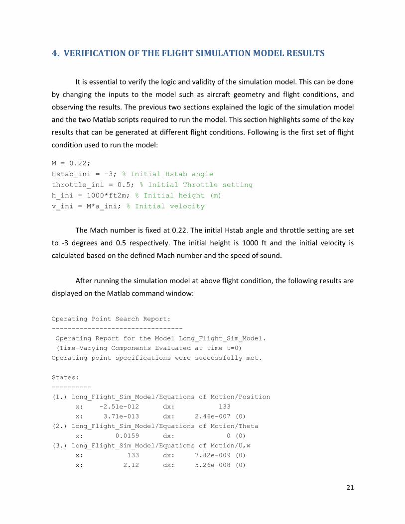
4. VERIFICATION OF THE FLIGHT SIMULATION MODEL RESULTS

It is essential to verify the logic and validity of the simulation model. This can be done

by changing the inputs to the model such as aircraft geometry and flight conditions, and

observing the results. The previous two sections explained the logic of the simulation model

and the two Matlab scripts required to run the model. This section highlights some of the key

results that can be generated at different flight conditions. Following is the first set of flight

condition used to run the model:

M = 0.22;

Hstab_ini = -3; % Initial Hstab angle

throttle_ini = 0.5; % Initial Throttle setting

h_ini = 1000*ft2m; % Initial height (m)

v_ini = M*a_ini; % Initial velocity

The Mach number is fixed at 0.22. The initial Hstab angle and throttle setting are set

to -3 degrees and 0.5 respectively. The initial height is 1000 ft and the initial velocity is

calculated based on the defined Mach number and the speed of sound.

After running the simulation model at above flight condition, the following results are

displayed on the Matlab command window:

Operating Point Search Report:

---------------------------------

Operating Report for the Model Long_Flight_Sim_Model.

(Time-Varying Components Evaluated at time t=0)

Operating point specifications were successfully met.

States:

----------

(1.) Long_Flight_Sim_Model/Equations of Motion/Position

x: -2.51e-012 dx: 133

x: 3.71e-013 dx: 2.46e-007 (0)

(2.) Long_Flight_Sim_Model/Equations of Motion/Theta

x: 0.0159 dx: 0 (0)

(3.) Long_Flight_Sim_Model/Equations of Motion/U,w

x: 133 dx: 7.82e-009 (0)

x: 2.12 dx: 5.26e-008 (0)

22

(4.) Long_Flight_Sim_Model/Equations of Motion/q

x: 0 dx: -8.16e-008 (0)

Inputs:

----------

(1.) Long_Flight_Sim_Model/Hstab

u: -1.1 [-Inf Inf]

(2.) Long_Flight_Sim_Model/Throttle

u: 0.5 [-Inf Inf]

Outputs: None

----------

Eigenvalue Damping Freq. (rad/s)

-1.25e+000 + 6.92e+000i 1.77e-001 7.03e+000

-1.25e+000 - 6.92e+000i 1.77e-001 7.03e+000

-1.78e-003 + 8.71e-002i 2.05e-002 8.71e-002

-1.78e-003 - 8.71e-002i 2.05e-002 8.71e-002

>> A

A =

0.0023 -0.2579 -2.8769 -9.8088

-0.0857 -2.3677 158.6155 -0.1563

0.0049 -0.3101 -0.1309 0

0 0 1.0000 0

>> CMalpha_model =

-1.0239

>> VH_bar =

0.0854

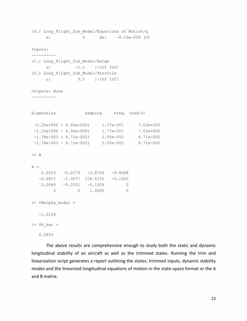
The above results are comprehensive enough to study both the static and dynamic

longitudinal stability of an aircraft as well as the trimmed states. Running the trim and

linearization script generates a report outlining the states, trimmed inputs, dynamic stability

modes and the linearized longitudinal equations of motion in the state-space format or the A

and B matrix.

23

TRIMMED INPUTS

The simulation model results provide the trimmed inputs namely the throttle setting

and Hstab angle, the two inputs of the simulation model. For example, the trimmed Hstab

angle is -1.1 deg and the throttle setting is 0.5 for steady motion of aircraft.

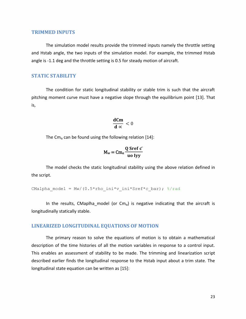
STATIC STABILITY

The condition for static longitudinal stability or stable trim is such that the aircraft

pitching moment curve must have a negative slope through the equilibrium point [13]. That

is,

The Cmα can be found using the following relation [14]:

Mw = Cmα

The model checks the static longitudinal stability using the above relation defined in

the script.

CMalpha_model = Mw/(0.5*rho_ini*v_ini*Sref*c_bar); %/rad

In the results, CMaplha_model (or Cmα) is negative indicating that the aircraft is

longitudinally statically stable.

LINEARIZED LONGITUDINAL EQUATIONS OF MOTION The primary reason to solve the equations of motion is to obtain a mathematical

description of the time histories of all the motion variables in response to a control input.

This enables an assessment of stability to be made. The trimming and linearization script

described earlier finds the longitudinal response to the Hstab input about a trim state. The

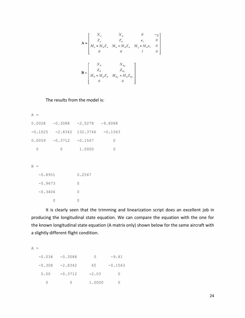
longitudinal state equation can be written as [15]:

24

The results from the model is:

A =

0.0028 -0.3088 -2.5278 -9.8088

-0.1025 -2.8342 132.3746 -0.1563

0.0059 -0.3712 -0.1567 0

0 0 1.0000 0

B =

-0.8951 0.2567

-0.9673 0

-0.3406 0

0 0

It is clearly seen that the trimming and linearization script does an excellent job in

producing the longitudinal state equation. We can compare the equation with the one for

the known longitudinal state equation (A matrix only) shown below for the same aircraft with

a slightly different flight condition.

A =

-0.034 -0.3088 0 -9.81

-0.308 -2.8342 65 -0.1563

0.00 -0.3712 -2.03 0

0 0 1.0000 0

25

It is important to discuss the variation in results. Firstly the dimensional derivatives

are calculated based on the operating point where trimming is done or a trimmed input is

determined. The script has a greater range of aerodynamic data to utilize and calculate the

dimensional derivatives. As discussed earlier, the aerodynamic data is not very accurate for

the geometry of the given aircraft. Moreover, the thrust is different in our case.

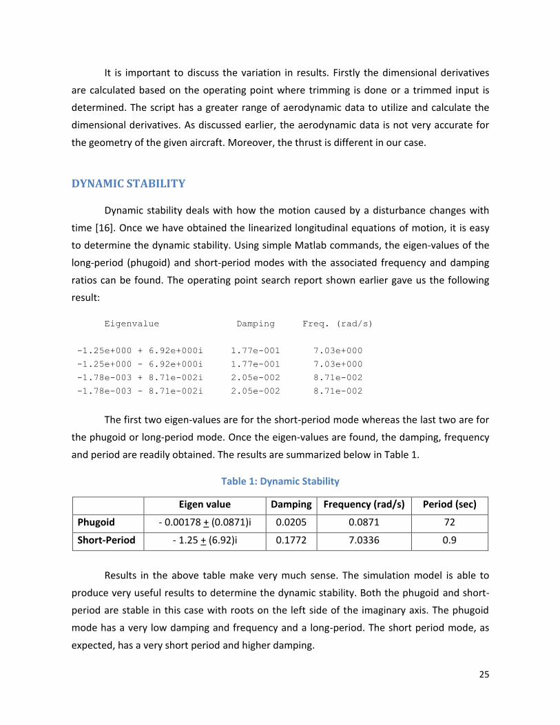
DYNAMIC STABILITY Dynamic stability deals with how the motion caused by a disturbance changes with

time [16]. Once we have obtained the linearized longitudinal equations of motion, it is easy

to determine the dynamic stability. Using simple Matlab commands, the eigen-values of the

long-period (phugoid) and short-period modes with the associated frequency and damping

ratios can be found. The operating point search report shown earlier gave us the following

result:

Eigenvalue Damping Freq. (rad/s)

-1.25e+000 + 6.92e+000i 1.77e-001 7.03e+000

-1.25e+000 - 6.92e+000i 1.77e-001 7.03e+000

-1.78e-003 + 8.71e-002i 2.05e-002 8.71e-002

-1.78e-003 - 8.71e-002i 2.05e-002 8.71e-002

The first two eigen-values are for the short-period mode whereas the last two are for

the phugoid or long-period mode. Once the eigen-values are found, the damping, frequency

and period are readily obtained. The results are summarized below in Table 1.

Table 1: Dynamic Stability

Eigen value Damping Frequency (rad/s) Period (sec)

Phugoid - 0.00178 + (0.0871)i 0.0205 0.0871 72

Short-Period - 1.25 + (6.92)i 0.1772 7.0336 0.9

Results in the above table make very much sense. The simulation model is able to

produce very useful results to determine the dynamic stability. Both the phugoid and short-

period are stable in this case with roots on the left side of the imaginary axis. The phugoid

mode has a very low damping and frequency and a long-period. The short period mode, as

expected, has a very short period and higher damping.

26

HORIZONTAL TAIL-VOLUME RATIO VH

The horizontal tail-volume ratio H is a very important parameter in stability and

control studies. The trimming and linearization script calculates H every time it is run using

the following relation [17].

=

All the variables of H such as lt, St, Sref and will be varied to perform various

simulation cases as described in the next section.

27

SIMULATION CASES

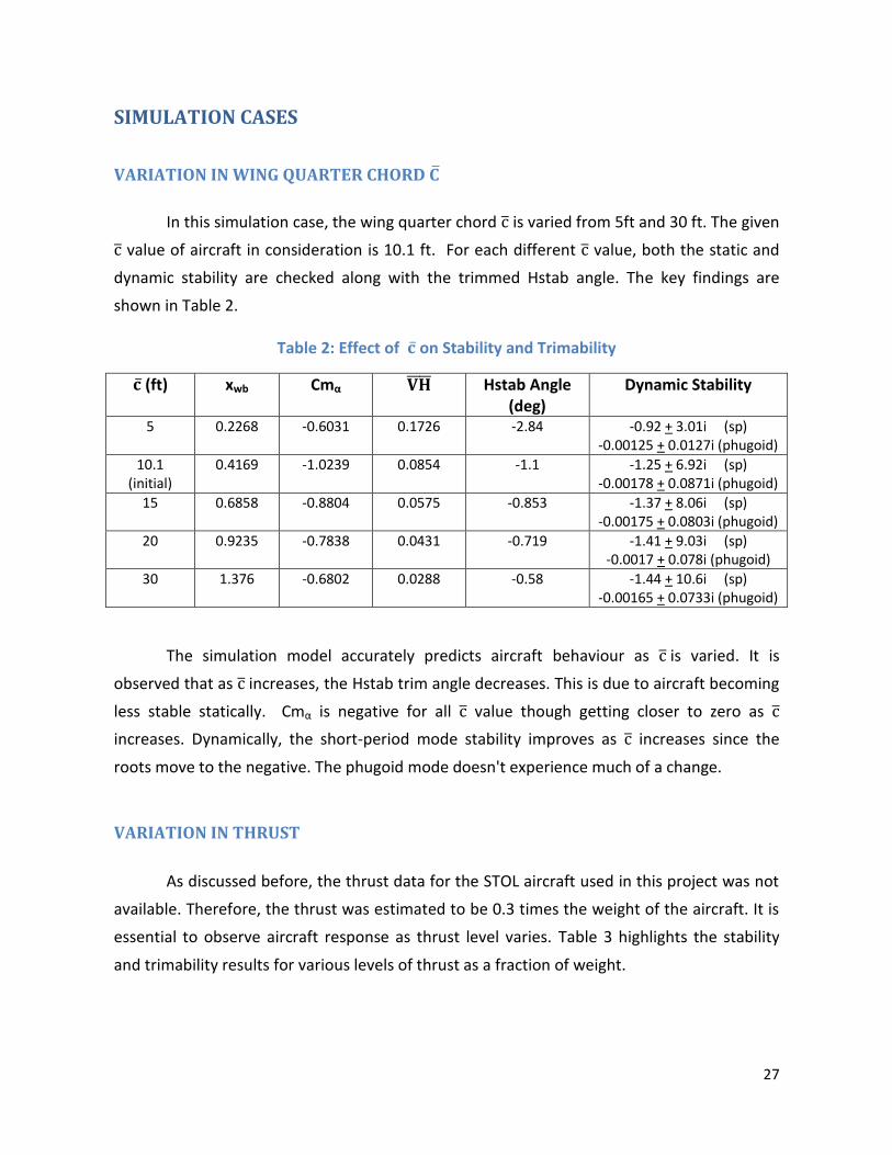
VARIATION IN WING QUARTER CHORD

In this simulation case, the wing quarter chord is varied from 5ft and 30 ft. The given

value of aircraft in consideration is 10.1 ft. For each different value, both the static and

dynamic stability are checked along with the trimmed Hstab angle. The key findings are

shown in Table 2.

Table 2: Effect of on Stability and Trimability

(ft) xwb Cmα

Hstab Angle (deg)

Dynamic Stability

5 0.2268 -0.6031 0.1726 -2.84 -0.92 + 3.01i (sp) -0.00125 + 0.0127i (phugoid)

10.1 (initial)

0.4169 -1.0239 0.0854 -1.1 -1.25 + 6.92i (sp) -0.00178 + 0.0871i (phugoid)

15 0.6858 -0.8804 0.0575 -0.853 -1.37 + 8.06i (sp) -0.00175 + 0.0803i (phugoid)

20 0.9235 -0.7838 0.0431 -0.719 -1.41 + 9.03i (sp) -0.0017 + 0.078i (phugoid)

30 1.376 -0.6802 0.0288 -0.58 -1.44 + 10.6i (sp) -0.00165 + 0.0733i (phugoid)

The simulation model accurately predicts aircraft behaviour as is varied. It is

observed that as increases, the Hstab trim angle decreases. This is due to aircraft becoming

less stable statically. Cmα is negative for all value though getting closer to zero as

increases. Dynamically, the short-period mode stability improves as increases since the

roots move to the negative. The phugoid mode doesn't experience much of a change.

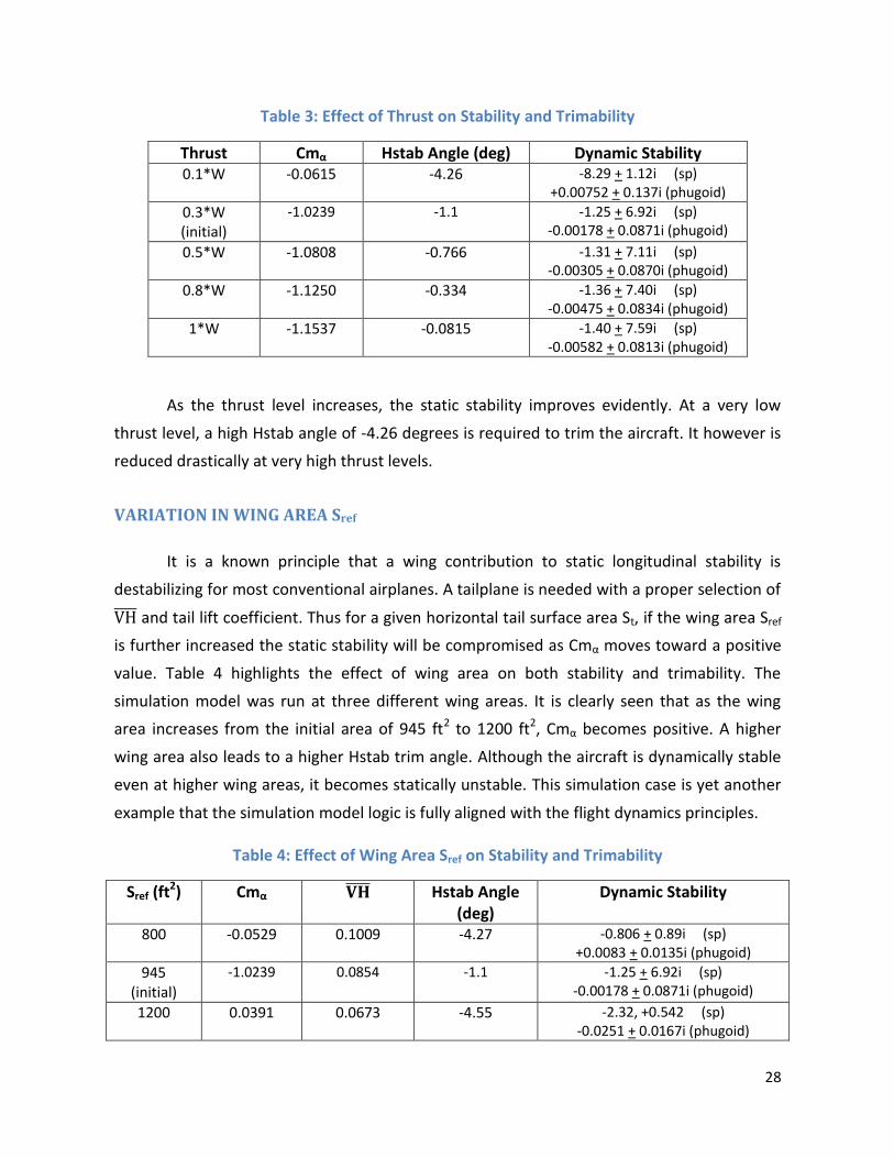
VARIATION IN THRUST

As discussed before, the thrust data for the STOL aircraft used in this project was not

available. Therefore, the thrust was estimated to be 0.3 times the weight of the aircraft. It is

essential to observe aircraft response as thrust level varies. Table 3 highlights the stability

and trimability results for various levels of thrust as a fraction of weight.

28

Table 3: Effect of Thrust on Stability and Trimability

Thrust Cmα Hstab Angle (deg) Dynamic Stability 0.1*W -0.0615 -4.26 -8.29 + 1.12i (sp)

+0.00752 + 0.137i (phugoid) 0.3*W (initial)

-1.0239 -1.1 -1.25 + 6.92i (sp) -0.00178 + 0.0871i (phugoid)

0.5*W -1.0808 -0.766 -1.31 + 7.11i (sp) -0.00305 + 0.0870i (phugoid)

0.8*W -1.1250 -0.334 -1.36 + 7.40i (sp) -0.00475 + 0.0834i (phugoid)

1*W -1.1537 -0.0815 -1.40 + 7.59i (sp) -0.00582 + 0.0813i (phugoid)

As the thrust level increases, the static stability improves evidently. At a very low

thrust level, a high Hstab angle of -4.26 degrees is required to trim the aircraft. It however is

reduced drastically at very high thrust levels.

VARIATION IN WING AREA Sref

It is a known principle that a wing contribution to static longitudinal stability is

destabilizing for most conventional airplanes. A tailplane is needed with a proper selection of

H and tail lift coefficient. Thus for a given horizontal tail surface area St, if the wing area Sref

is further increased the static stability will be compromised as Cmα moves toward a positive

value. Table 4 highlights the effect of wing area on both stability and trimability. The

simulation model was run at three different wing areas. It is clearly seen that as the wing

area increases from the initial area of 945 ft2 to 1200 ft2, Cmα becomes positive. A higher

wing area also leads to a higher Hstab trim angle. Although the aircraft is dynamically stable

even at higher wing areas, it becomes statically unstable. This simulation case is yet another

example that the simulation model logic is fully aligned with the flight dynamics principles.

Table 4: Effect of Wing Area Sref on Stability and Trimability

Sref (ft2) Cmα Hstab Angle

(deg) Dynamic Stability

800 -0.0529 0.1009 -4.27 -0.806 + 0.89i (sp) +0.0083 + 0.0135i (phugoid)

945 (initial)

-1.0239 0.0854 -1.1 -1.25 + 6.92i (sp) -0.00178 + 0.0871i (phugoid)

1200 0.0391 0.0673 -4.55 -2.32, +0.542 (sp) -0.0251 + 0.0167i (phugoid)

29

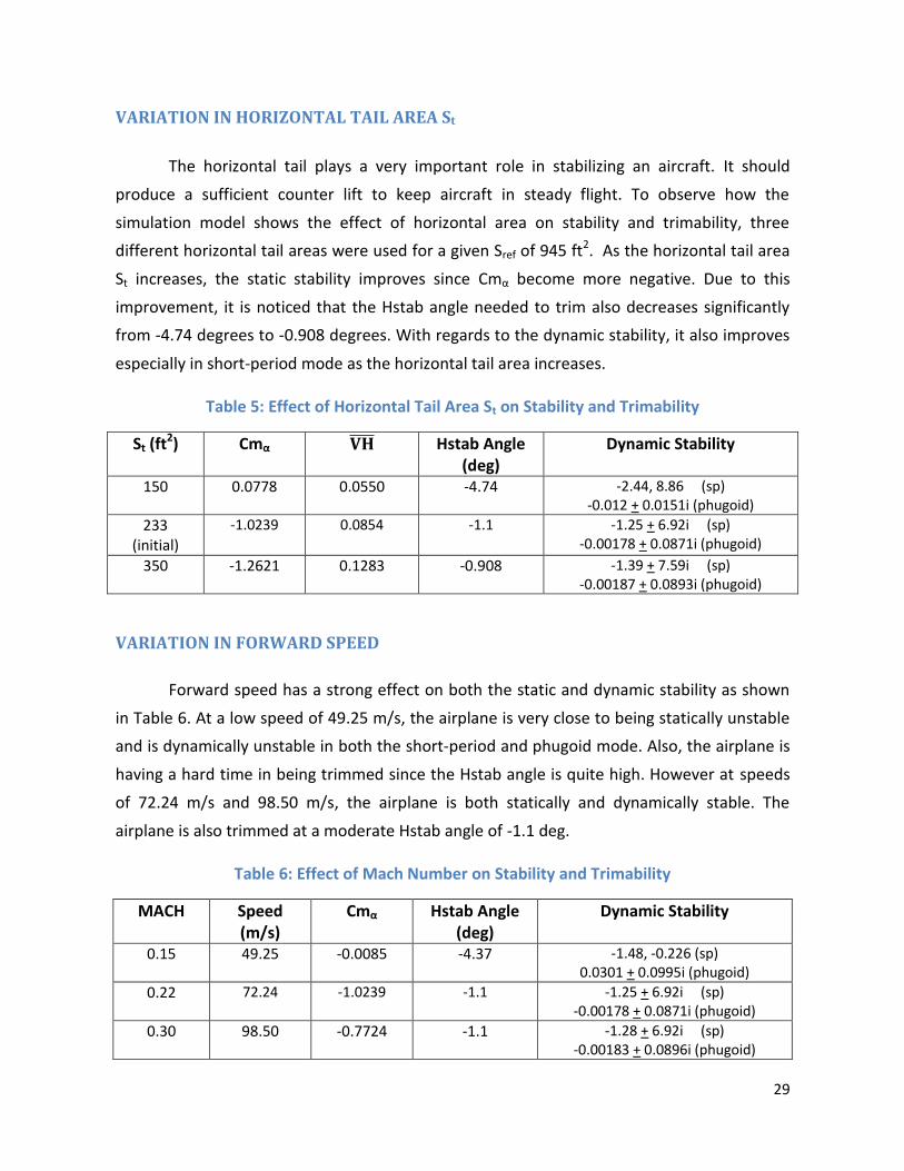
VARIATION IN HORIZONTAL TAIL AREA St

The horizontal tail plays a very important role in stabilizing an aircraft. It should

produce a sufficient counter lift to keep aircraft in steady flight. To observe how the

simulation model shows the effect of horizontal area on stability and trimability, three

different horizontal tail areas were used for a given Sref of 945 ft2. As the horizontal tail area

St increases, the static stability improves since Cmα become more negative. Due to this

improvement, it is noticed that the Hstab angle needed to trim also decreases significantly

from -4.74 degrees to -0.908 degrees. With regards to the dynamic stability, it also improves

especially in short-period mode as the horizontal tail area increases.

Table 5: Effect of Horizontal Tail Area St on Stability and Trimability

St (ft2) Cmα

Hstab Angle

(deg) Dynamic Stability

150 0.0778 0.0550 -4.74 -2.44, 8.86 (sp) -0.012 + 0.0151i (phugoid)

233 (initial)

-1.0239 0.0854 -1.1 -1.25 + 6.92i (sp) -0.00178 + 0.0871i (phugoid)

350 -1.2621 0.1283 -0.908 -1.39 + 7.59i (sp) -0.00187 + 0.0893i (phugoid)

VARIATION IN FORWARD SPEED

Forward speed has a strong effect on both the static and dynamic stability as shown

in Table 6. At a low speed of 49.25 m/s, the airplane is very close to being statically unstable

and is dynamically unstable in both the short-period and phugoid mode. Also, the airplane is

having a hard time in being trimmed since the Hstab angle is quite high. However at speeds

of 72.24 m/s and 98.50 m/s, the airplane is both statically and dynamically stable. The

airplane is also trimmed at a moderate Hstab angle of -1.1 deg.

Table 6: Effect of Mach Number on Stability and Trimability

MACH Speed (m/s)

Cmα Hstab Angle (deg)

Dynamic Stability

0.15 49.25 -0.0085 -4.37 -1.48, -0.226 (sp) 0.0301 + 0.0995i (phugoid)

0.22 72.24 -1.0239 -1.1 -1.25 + 6.92i (sp) -0.00178 + 0.0871i (phugoid)

0.30 98.50 -0.7724 -1.1 -1.28 + 6.92i (sp) -0.00183 + 0.0896i (phugoid)

30

5. CONCLUSION AND RECOMMENDATIONS

A basic 3-DoF longitudinal flight simulation model has been built to study behaviour

of an aircraft in this project. The simulation model is comprehensive and can determine both

the static and dynamic stability of an aircraft. The model also trims the airplane motion and

finds the trimmed inputs. The mass properties and geometric data of a generic STOL aircraft

were used to predict the aerodynamic behaviour of aircraft. AVL software, an alternative of

Datcom, was utilized to produce the aerodynamic data required in the simulation model. The

simulation model consisted of three blocks namely Aerodynamic, Thrust and Equations of

Motion blocks. These blocks are linked together to form an integrated longitudinal flight

simulation model. Initialization script and Trimming and Linearization script were the two

scripts used to run the simulation model. The initialization script initialized all the parameters

needed prior to simulation and the other script linearized equations of motion and provided

the trimmed solution. The results were generated in the form of a report that consisted of

trimmed inputs, longitudinal equations of motion (A and B matrix), static stability in the form

of Cmα and the dynamic stability in the form of roots for both the short-period and phugoid

modes. Moreover, various parameters such as aircraft geometry and flight conditions were

changed to run the simulation model. The objective was to test the simulation model

capability in producing results for different cases. It was observed that the model was

successful in accurately predicting the aircraft behavior as either the geometric data or flight

condition varied since the flight dynamics principles were not violated. For instance, as the

horizontal tail area increases, we expect the horizontal stabilizer angle to reduce. This was

successfully predicted by the model. Similarly, various results when obtained for cases in

which thrust, wing area, wing quarter chord and Mach number were varied. Both the static

and dynamic stability in each of the cases were also studied.

It is pertinent to mention that the flight simulation model designed is quite generic in

nature and can be used to simulate the behavior of any aircraft. Moreover, the simulation

model can be extended to serve any objective. It contains the essential elements or systems

of an aircraft that play the most crucial role in any flight simulation model. For instance, the

focal point of any flight simulator is the equations of motion block that requires accurate

inputs from aerodynamics and propulsion models. Thus this report places an important

31

emphasis on both models. Another salient feature of the flight simulation model is that it is

comprehensive enough to conduct the longitudinal stability analysis.

The question arises as to how the simulation model can be useful for a designer who

intends to design a new aircraft and would want to study basic aircraft behavior. As stated in

the section of engineering flight simulation methodology, the process would start by first

establishing the system level requirements for the new aircraft and defining the preliminary

geometry. Once the geometric configuration is known, the Datcom or AVL program can be

used to calculate the aerodynamic characteristics. The aerodynamic data can then be

transferred to the look-up tables of the Aerodynamics Block of the simulation model. Once

the Block is filled with relevant data, the equations of motion can be solved for longitudinal

motion. Moreover, the fidelity of the simulation model can be increased by incorporating the

6-DOF model interface. The simulation model of a new aircraft can also be used for

entertainment purposes. A joystick can be used to input commands to the pilot model. An

interface of MATLAB/Simulink with FlightGear can be created and a script can be run to play

in real time. Introduction of a joystick is the first step of introducing an actual hardware into

the model.

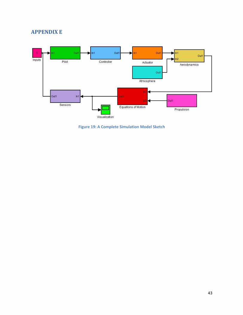
The simulation model can be further extended to include some other systems to

assess airplane handling characteristics. This would require pilot system along with actuator

and control systems. Moreover, a sensor block can be added to as a feedback to pilot block

and making the simulation model a closed loop system. Figure 19 in appendix E shows a

complete simulation model sketch or workflow that includes most of the essential simulation

elements or blocks such as pilot, controller, actuator, aerodynamics, atmosphere, propulsion,

equations of motion and sensors. Other blocks that can be added are landing gear and aero

elastic loads.

Finally, the limitations of the flight simulation model should be properly understood

in order to improve it. The main area of improvement in the simulation model lies in the

Aerodynamic Model. Although AVL provides the basic data for analysis, experimentally

determining the aerodynamics coefficients should be the next step to validate AVL results.

Another key area is to develop a visualization path to visualize results. This requires

installation of FlightGear with high performance graphics card and a valid interface with

MATLAB/Simulink. Flight sensors are an excellent way of validating the model due to their

32

feedback information. In essence, the flight simulation model developed in this project can

be used as a solid foundation for any simulation study.

33

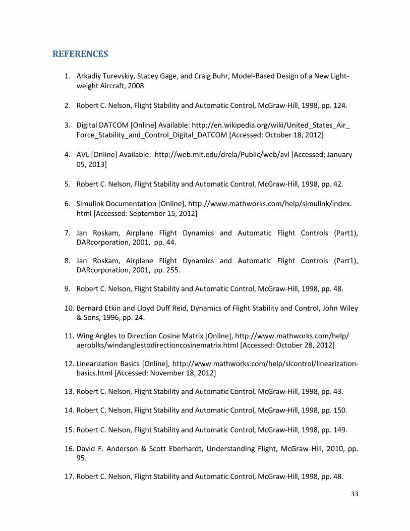
REFERENCES

1. Arkadiy Turevskiy, Stacey Gage, and Craig Buhr, Model-Based Design of a New Light- weight Aircraft, 2008

2. Robert C. Nelson, Flight Stability and Automatic Control, McGraw-Hill, 1998, pp. 124.

3. Digital DATCOM [Online] Available: http://en.wikipedia.org/wiki/United_States_Air_ Force_Stability_and_Control_Digital_DATCOM [Accessed: October 18, 2012]

4. AVL [Online] Available: http://web.mit.edu/drela/Public/web/avl [Accessed: January 05, 2013]


6. Simulink Documentation [Online], http://www.mathworks.com/help/simulink/index. html [Accessed: September 15, 2012]

7. Jan Roskam, Airplane Flight Dynamics and Automatic Flight Controls (Part1), DARcorporation, 2001, pp. 44.

8. Jan Roskam, Airplane Flight Dynamics and Automatic Flight Controls (Part1), DARcorporation, 2001, pp. 255.


10. Bernard Etkin and Lloyd Duff Reid, Dynamics of Flight Stability and Control, John Wiley & Sons, 1996, pp. 24.

11. Wing Angles to Direction Cosine Matrix [Online], http://www.mathworks.com/help/ aeroblks/windanglestodirectioncosinematrix.html [Accessed: October 28, 2012]

12. Linearization Basics [Online], http://www.mathworks.com/help/slcontrol/linearization-basics.html [Accessed: November 18, 2012]




16. David F. Anderson & Scott Eberhardt, Understanding Flight, McGraw-Hill, 2010, pp. 95.


34

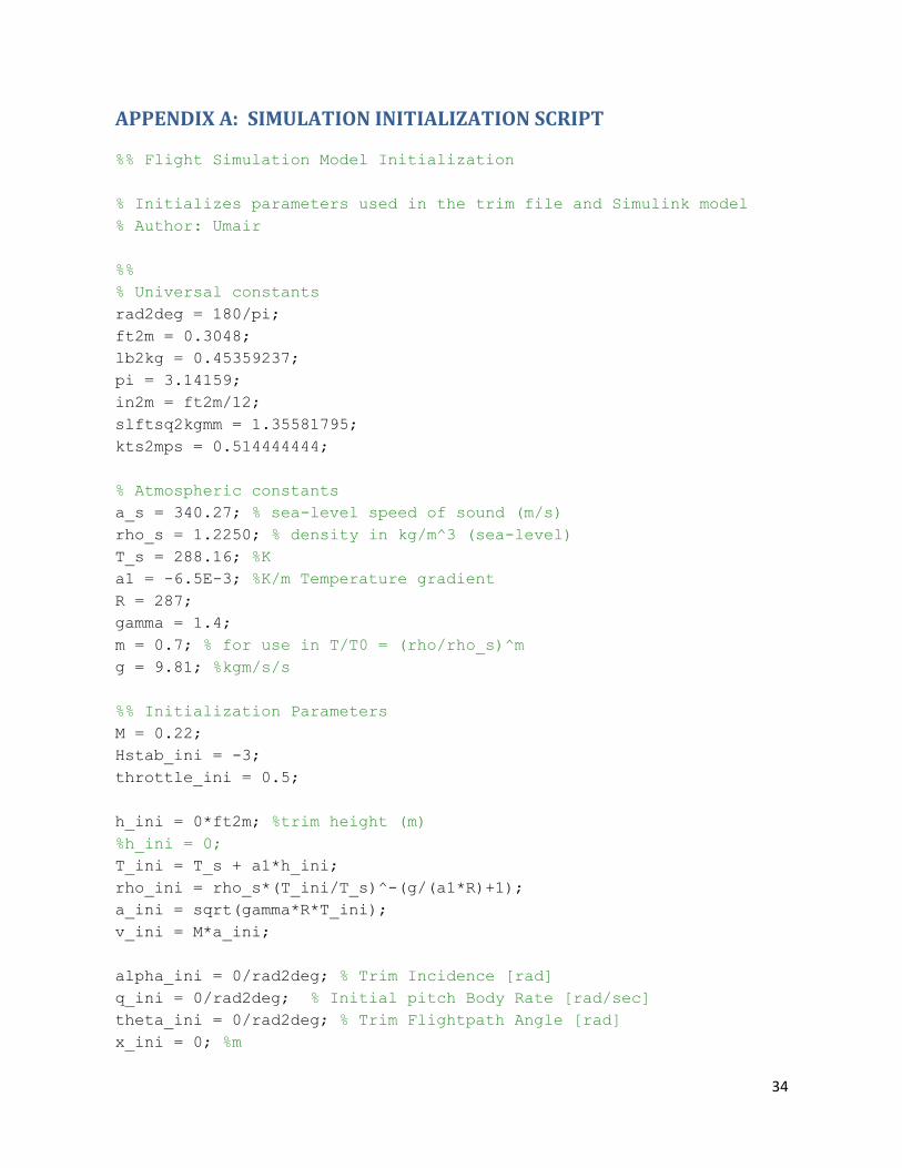
APPENDIX A: SIMULATION INITIALIZATION SCRIPT

%% Flight Simulation Model Initialization

% Initializes parameters used in the trim file and Simulink model

% Author: Umair

%%

% Universal constants

rad2deg = 180/pi;

ft2m = 0.3048;

lb2kg = 0.45359237;

pi = 3.14159;

in2m = ft2m/12;

slftsq2kgmm = 1.35581795;

kts2mps = 0.514444444;

% Atmospheric constants

a_s = 340.27; % sea-level speed of sound (m/s)

rho_s = 1.2250; % density in kg/m^3 (sea-level)

T_s = 288.16; %K

a1 = -6.5E-3; %K/m Temperature gradient

R = 287;

gamma = 1.4;

m = 0.7; % for use in T/T0 = (rho/rho_s)^m

g = 9.81; %kgm/s/s

%% Initialization Parameters

M = 0.22;

Hstab_ini = -3;

throttle_ini = 0.5;

h_ini = 0*ft2m; %trim height (m)

%h_ini = 0;

T_ini = T_s + a1*h_ini;

rho_ini = rho_s*(T_ini/T_s)^-(g/(a1*R)+1);

a_ini = sqrt(gamma*R*T_ini);

v_ini = M*a_ini;

alpha_ini = 0/rad2deg; % Trim Incidence [rad]

q_ini = 0/rad2deg; % Initial pitch Body Rate [rad/sec]

theta_ini = 0/rad2deg; % Trim Flightpath Angle [rad]

x_ini = 0; %m

35

pos_ini = [x_ini -h_ini];

U0 = v_ini*cos(alpha_ini);%m/s

w0 = v_ini*sin(alpha_ini); %m/s

%% Aircraft Mass and Geometry Data

mass = 40000*lb2kg;

CG = 40; % CG location

Iyy=21500*slftsq2kgmm;

St = 233*ft2m*ft2m; %H tail area (in m^2)

Sref = 945*ft2m*ft2m; %Wing area (in m^2)

lt = 3.5*ft2m; % distance of tail from c.g.(m)

zt = 1.2*ft2m;

bt = 32*ft2m; % Tail span (m)

c_bar = 10.1*ft2m; % wing MAC (m)

xwb = (CG-25)/100*c_bar; % x-distance between CG and quarter chord

zwb = 0; % neglected

%engine

%T/W ratio = 0.3

% Assume T constant with speed, otherwise, find T/T0 = AM^-n, with A

and n

% constants for specific engine

Static_Thrust = 0.3*mass; % N

36

APPENDIX B: TRIMMING AND LINEARIZATION SCRIPT

%% Longitudinal Flight Simulation trim file

% Perform linearization and trim for Longitudinal Flight Simulation

Model using data

%% Set Operating Point and State Specifications

% The first state specifications are Position states, the second

state specification is Theta. Both are known, but not at steady

state.

% The third state specifications are body axis angular rates of which

the variable w is at steady state.

opspec = operspec('Long_Flight_Sim_Model');

opspec.State(1).Known = [0;0];

opspec.State(1).SteadyState = [0;1];

opspec.State(2).Known = 0;

opspec.State(2).SteadyState = 1;

opspec.State(3).Known = [0;0];

opspec.State(3).SteadyState = [1;1];

opspec.State(4).Known = 1;

opspec.State(4).SteadyState = 1;

opspec.Input(1).Known = 0;

opspec.Input(2).Known = 0;

opspec.Input(1).u = Hstab_ini;

opspec.Input(2).u = throttle_ini;

%% Search for Operating Point, Set I/O, then Linearize

op = findop('Long_Flight_Sim_Model',opspec);

io(1) = linio('Long_Flight_Sim_Model/Hstab',1,'in'); %tail plane

angle input (deg)

io(2) = linio('Long_Flight_Sim_Model/Throttle',1,'in'); % Throttle

command since it is modeled as a multiplicator to Thrust available,

should be between 0 and 1

io(3) = linio('Long_Flight_Sim_Model/Equations of Motion',1,'out'); %

Theta

37

io(4) = linio('Long_Flight_Sim_Model/Equations of Motion',2,'out'); %

q

io(5) = linio('Long_Flight_Sim_Model/Selector',1,'out'); % U

io(6) = linio('Long_Flight_Sim_Model/Selector1',1,'out'); % w

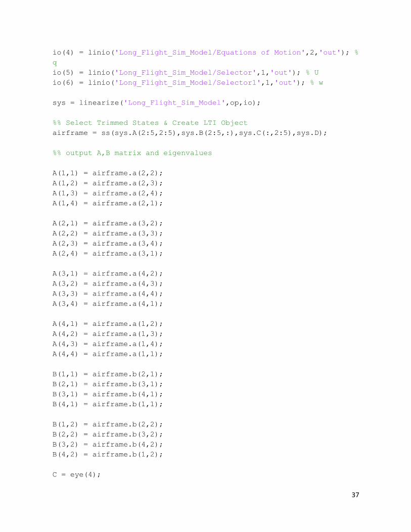
sys = linearize('Long_Flight_Sim_Model',op,io);

%% Select Trimmed States & Create LTI Object

airframe = ss(sys.A(2:5,2:5),sys.B(2:5,:),sys.C(:,2:5),sys.D);

%% output A,B matrix and eigenvalues

A(1,1) = airframe.a(2,2);
















B(1,1) = airframe.b(2,1);








C = eye(4);

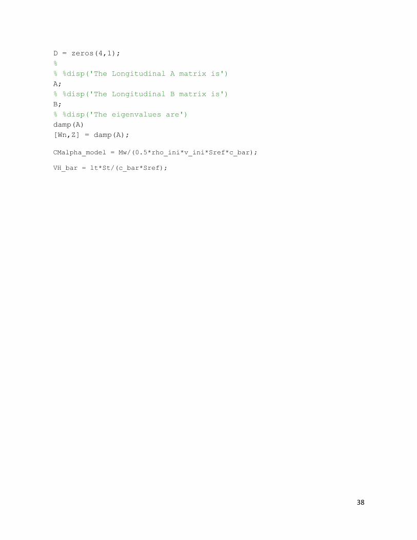
38

D = zeros(4,1);

%

% %disp('The Longitudinal A matrix is')

A;

% %disp('The Longitudinal B matrix is')

B;

% %disp('The eigenvalues are')

damp(A)

[Wn,Z] = damp(A);

CMalpha_model = Mw/(0.5*rho_ini*v_ini*Sref*c_bar);

VH_bar = lt*St/(c_bar*Sref);

39

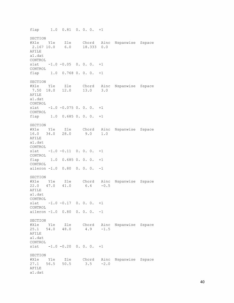
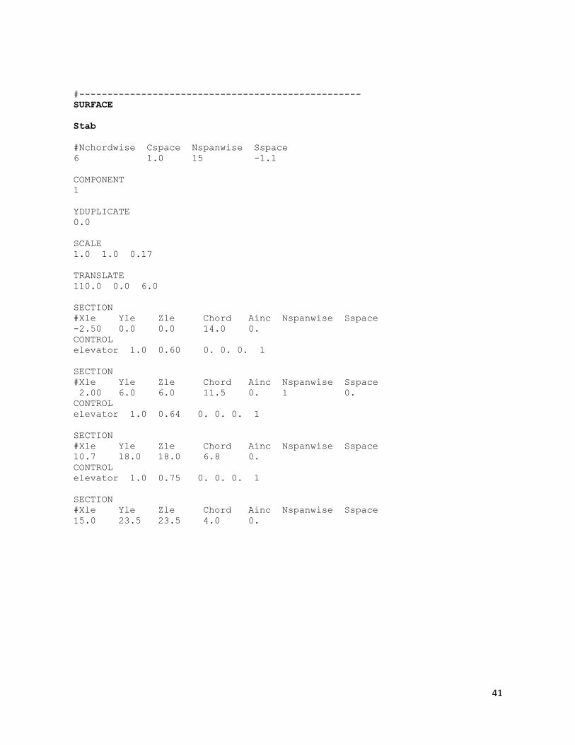
APPENDIX C: AVL GEOMETRIC INPUT FILE FOR DATA CALCULATION

STOL

#Mach

0.22

#IYsym IZsym Zsym

0 0 0.0

#Sref Cref Bref

945.0 10.1 233.0

#Xref Yref Zref

40.0 0.0 0.0

#--------------------------------------------------

SURFACE

Wing

!Nchordwise Cspace Nspanwise Sspace

12 1.0 26 -1.1

COMPONENT

1

YDUPLICATE

0.0

ANGLE

0.0

SCALE

1.0 1.0 0.07

TRANSLATE

50.0 0.0 0.0

!SECTION

!#Xle Yle Zle Chord Ainc Nspanwise Sspace

!-0.5 0.0 0.0 21.0 5.0

!AFILE

!a1.dat

!CONTROL

!flap 1.0 0.81 0. 0. 0. +1

SECTION

#Xle Yle Zle Chord Ainc Nspanwise Sspace

-0.5 6.0 0.0 21.0 5.0

AFILE

a1.dat

CONTROL

slat -1.0 -0.05 0. 0. 0. +1

CONTROL

40

flap 1.0 0.81 0. 0. 0. +1

SECTION


2.167 10.0 6.0 18.333 0.0

AFILE

a1.dat

CONTROL

slat -1.0 -0.05 0. 0. 0. +1

CONTROL

flap 1.0 0.768 0. 0. 0. +1

SECTION


7.50 18.0 12.0 13.0 3.0

AFILE

a1.dat

CONTROL

slat -1.0 -0.075 0. 0. 0. +1

CONTROL

flap 1.0 0.685 0. 0. 0. +1

SECTION


16.0 34.0 28.0 9.0 1.0

AFILE

a1.dat

CONTROL

slat -1.0 -0.11 0. 0. 0. +1

CONTROL

flap 1.0 0.685 0. 0. 0. +1

CONTROL

aileron -1.0 0.80 0. 0. 0. -1

SECTION


22.0 47.0 41.0 6.4 -0.5

AFILE

a1.dat

CONTROL

slat -1.0 -0.17 0. 0. 0. +1

CONTROL

aileron -1.0 0.80 0. 0. 0. -1

SECTION


25.1 54.0 48.0 4.9 -1.5

AFILE

a1.dat

CONTROL

slat -1.0 -0.20 0. 0. 0. +1

SECTION


27.1 56.5 50.5 3.5 -2.0

AFILE

a1.dat

41

#--------------------------------------------------

SURFACE

Stab

#Nchordwise Cspace Nspanwise Sspace

6 1.0 15 -1.1

COMPONENT

1

YDUPLICATE

0.0

SCALE

1.0 1.0 0.17

TRANSLATE

110.0 0.0 6.0

SECTION


-2.50 0.0 0.0 14.0 0.

CONTROL

elevator 1.0 0.60 0. 0. 0. 1

SECTION


2.00 6.0 6.0 11.5 0. 1 0.

CONTROL

elevator 1.0 0.64 0. 0. 0. 1

SECTION


10.7 18.0 18.0 6.8 0.

CONTROL

elevator 1.0 0.75 0. 0. 0. 1

SECTION


15.0 23.5 23.5 4.0 0.

42

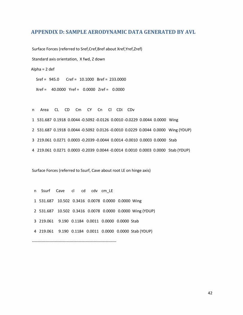
APPENDIX D: SAMPLE AERODYNAMIC DATA GENERATED BY AVL

Surface Forces (referred to Sref,Cref,Bref about Xref,Yref,Zref)

Standard axis orientation, X fwd, Z down

Alpha = 2 def

Sref = 945.0 Cref = 10.1000 Bref = 233.0000

Xref = 40.0000 Yref = 0.0000 Zref = 0.0000

n Area CL CD Cm CY Cn Cl CDi CDv

1 531.687 0.1918 0.0044 -0.5092 -0.0126 0.0010 -0.0229 0.0044 0.0000 Wing

2 531.687 0.1918 0.0044 -0.5092 0.0126 -0.0010 0.0229 0.0044 0.0000 Wing (YDUP)

3 219.061 0.0271 0.0003 -0.2039 -0.0044 0.0014 -0.0010 0.0003 0.0000 Stab

4 219.061 0.0271 0.0003 -0.2039 0.0044 -0.0014 0.0010 0.0003 0.0000 Stab (YDUP)

Surface Forces (referred to Ssurf, Cave about root LE on hinge axis)

n Ssurf Cave cl cd cdv cm_LE

1 531.687 10.502 0.3416 0.0078 0.0000 0.0000 Wing

2 531.687 10.502 0.3416 0.0078 0.0000 0.0000 Wing (YDUP)

3 219.061 9.190 0.1184 0.0011 0.0000 0.0000 Stab

4 219.061 9.190 0.1184 0.0011 0.0000 0.0000 Stab (YDUP)

---------------------------------------------------------------

43

APPENDIX E

Figure 19: A Complete Simulation Model Sketch

Documents

3-DOF Longitudinal Flight Simulation Modeling and Design Using MA