Embed Size (px)
Citation preview
78:6 (2016) 117–137 | www.jurnalteknologi.utm.my | eISSN 2180–3722 |
Jurnal
Teknologi
Full Paper
DEVELOPMENT AND VERIFICATION OF A 9-
DOF ARMORED VEHICLE MODEL IN THE
LATERAL AND LONGITUDINAL DIRECTIONS
Vimal Rau Aparowa*, Khisbullah Hudhaa, Megat Mohamad
Hamdan Megat Ahmada, Hishamuddin Jamaluddinb
aDepartment of Mechanical Engineering, Faculty of
Engineering, National Defense University of Malaysia, Kem
Sungai Besi, Kuala Lumpur, Malaysia bDepartment of Applied Mechanics and Design, Faculty of
Mechanical Engineering, Universiti Teknologi Malaysia, 81310
UTM Johor Bahru, Johor, Malaysia
Article history
Received
19 Sepember 2015
Received in revised form
28 October 2015
Accepted
15 May 2016
*Corresponding author
Abstract
This manuscript presents the development of an armored vehicle model in lateral and longitudinal directions. A Nine Degree
of Freedom (9-DOF) armored vehicle model was derived mathematically and integrated with an analytical tire dynamics
known as Pacejka Magic Tire model. The armored vehicle model is developed using three main inputs of a vehicle system
which are Pitman arm steering system, Powertrain system and also hydraulic assisted brake system. Several testings in lateral
and longitudinal direction are performed such as double lane change, slalom, step steer and sudden acceleration and
sudden braking to verify the vehicle model. The armored vehicle model is verified using validated software, CarSim, using
HMMWV vehicle model as a benchmark. The verification responses show that the developed armored vehicle model can be
used for both lateral and longitudinal direction analysis
Keywords: 9-DOF, armored vehicle, lateral, longitudinal, HMMWV vehicle
Abstrak
Manuskrip ini membentangkan mengenai permodelan kenderaan kereta kebal pada arah ke sisi dan mendatar. Sembilan
darjah kebebasan ( 9-DOF ) model kenderaan kereta kebal telah diperoleh secara matematik dan bersepadu dengan
dinamik tayar analisis dikenali sebagai model Pacejka Magic tayar. Model kenderaan kereta kebal itu juga dibangunkan
dengan menggunakan tiga input utama system untuk kenderaan iaitu Pitman Arm sistem stereng, sistem enjin dan juga sistem
brek dengan menggunakan system hydralik. Beberapa ujian ke arah sisi dan memdatar telah dianalisasi dalam manuscript ini
seperti perubahan dua lorong, Slalom , langkah kemudi dan pecutan dan brek secara tiba-tiba untuk mengesahkan
kesahihkan model kenderaan tersebut. Model kenderaan ini dianalisasikan dengan menggunakan system perisian yang
disahkan, iaitu CarSim , dengan menggunakan kenderaan kereta kebal HMMWV sebagai rujukan utama. Hasil ujian-ujian ini
menunjukkan bahawa model kenderaan kereta kebal yang dibangunkan boleh digunakan untuk menganalisasi ciri-ciri
sebuah kenderan kereta kebal pada kedua-dua arah iaitu sisi dan mendatar.
Kata kunci: Sembilan darjah kebebasan, kereta kebal, sisi, memdatar, kereta HMMWV
© 2016 Penerbit UTM Press. All rights reserved
1.0 INTRODUCTION
Since past few decades, vehicle plays an important
role for every human in their daily life usage. Owning
personal vehicles not only will reduce time but also
save human energy to travel from one location to
another. However, this transportation has significantly
increased the risk of each human’s life due to road
accidents. The major cause of the vehicle accidents
is the non-stability conditions of a vehicle where the
118 Vimal Rau Aparow et al. / Jurnal Teknologi (Sciences & Engineering) 78:6 (2016) 117–137
drivers lost control while driving either by steering,
throttle or braking input [1]. Rollover and skidding are
known as a major effect occurs once the driver
unable to control the vehicle. Therefore, handling
and stability of each vehicle has become one of the
main priorities for the automotive developers during
analysis procedure.
The handling and stability performances are one
of the important milestones in developing a vehicle.
In order to reduce time and also the costing issue,
the automotive developers initiate their research
works by developing a vehicle model via computer-
based simulation technique. Most of the automotive
researchers developed the vehicle model using
mathematical derivation by describing them in terms
of degree of freedom (DOF). The advantage of using
this computer-based simulation technique is to study
and analyze the dynamic behavior of a vehicle
system by simulating into a mathematical model. The
simulation model can be evaluated using various
types of operating conditions and also able to make
appropriate adjustment to the vehicle model for
future improvement [2]. The simulation technique
also has great significance in reducing the cost for
test bed and testing instruments as for initial stage of
analysis since it does not require in simulation
techniques [3].
In recent years, most of the automotive
researchers extensively involved in the development
of vehicle model to analysis the dynamic behavior of
an actual vehicle. They have developed the vehicle
model as a simplified quarter and half vehicle model
or full vehicle model. In term of quarter vehicle model
in vertical direction, previous researchers have done
evaluation on the suspension system. Yoshimura et al.
[4] successfully developed an active suspension
system of a quarter vehicle model using sliding mode
control. Meanwhile, Litak et al. [5] and Turkay and
Akcay [6] studied on chaotic and random vibration
characteristic using a quarter vehicle model. Tusset
et al. [7] investigated the performance of
magnetorheological damper in quarter vehicle
model using an intelligent controller.
In the longitudinal direction of the vehicle model,
Jansen et al. [8] and Aparow et al. [9] studied on the
ABS performance using quarter vehicle model.
Furthermore, a regenerative braking system has been
tested using a quarter vehicle model [10].
Meanwhile, there are other researchers whom mainly
focus on the performance of the vehicle model in
lateral direction. Rauh [11] examined both ride and
handling performance by using a quarter vehicle
model. Similarly, Zin et al. [12] developed simplified
handling model known as 2 DOF bicycle model to
evaluate the performance of vehicle in handling and
suspension control. Meijaard and Schwab [13]
investigated bicycle model to study on the handling
performance due to the effect of a pneumatic trail
and a damping at the tire contact. Baslamisli et al.
[14] used bicycle model to develop active steering
system using gain scheduled method.
Nevertheless, other researchers have enhanced the
research scope to a higher degree of freedom such
as Thompson and Pearce [15] examined the
performance index for an optimal control for half
vehicle active suspension by using the spectral
decomposition method. Likewise, Gao et al. [16] also
investigated the dynamic performance of vehicle
under random road input excitations. Besides, a non-
linear control integrated with active suspension is
analysed on half vehicle model using road-adaptive
algorithm [17]. Studies on quarter and half vehicle
model have shown that the model is very useful in
various applications. However, these models do not
allow the automotive researchers to evaluate the
vehicle model in lateral and longitudinal direction
due to its limitation to include the steering, throttle
and brake input from the driver. Thus, the researchers
start to develop non-simplified vehicle model or
known as a full vehicle model.
A lot of researches have been developed by
previous researchers to analyze the performance of
vehicle model in lateral, longitudinal and vertical
direction. Ahmad et al. [18] have used 14-DOF
vehicle ride model to develop active suspension
using adaptive PID with pitch moment rejection
control. Meanwhile, 14-DOF vehicle handling model
has been used for active suspension system with roll
moment rejection control [19]. Aparow et al. [20] also
developed 5-DOF full vehicle model in longitudinal
direction to study on ABS performance. Besides,
Hudha et al. [21] also have examined the 12-DOF
ride model of an armored vehicle by controlling the
suspension system with effect from gun system and
also road irregularities. Similarly, Trikande et al. [22]
has studied 11 DOF armored vehicle on ride
performance of the model using semi-active
suspension due to the firing attack and instability of
the vehicle. However, all the previous studies have
analyzed the performance of the vehicle model only
in one direction by neglecting other direction. It
shows that the proposed vehicle model is applicable
for a single testing procedure only. Moreover, the
effect from steering inertia, effect of throttle torque
from engine and also surrounding disturbance are
mostly neglected while developing a full vehicle
model.
In order to overcome this shortcomings, a
combination of both lateral and longitudinal of
vehicle model has been developed in this study. The
developed vehicle model is mainly designed for
armored type of vehicle whereby the system
configuration of steering system is used based on
Pitman arm system and the internal combustion
engine is developed for the armored vehicle model
with an additional gun turret system is mounted on to
of the armored vehicle. Meanwhile, the hydraulic
brake actuator model is used in this study to
represent a simplified model of brake system
dynamics from a physical modeling [20]. The three
main inputs which are steering, throttling and braking
from the driver are used during testing in both
directions. The developed armored vehicle model is
119 Vimal Rau Aparow et al. / Jurnal Teknologi (Sciences & Engineering) 78:6 (2016) 117–137
evaluated using validated CarSim software on both
lateral and longitudinal direction. It demonstrates the
capability of the developed vehicle model to be
tested using more than single direction without
adjusting the subsystems or parameters
This paper is organized as follows: The first section
represents the introduction and review of some
related works. The second section is followed by
modeling the dynamic behavior of armored vehicle
model in lateral and longitudinal direction by
proposing Pajecka Magic formula as the tire model
and the vehicle input models such as Pitman Arm
steering system, powertrain and hydraulic assisted
brake model of an armored vehicle dynamic model.
The following section discusses the verification
procedure using validated CarSim software and
discuss about the performance of the armored
vehicle model in lateral and longitudinal direction.
The fifth section discusses the future work of proposed
armored vehicle model and finally is the conclusion
2.0 A 9 DOF ARMORED VEHICLE MODEL
A 9 DOF of an armored vehicle considered in this
study consists of a single sprung mass (vehicle body)
connected to four unsprung masses. The vehicle
model is developed by combining the lateral [23,24]
and longitudinal dynamic [20, 25] of the vehicle
model. Hence, this paper focuses on the
performance of an armored vehicle model in both
lateral and longitudinal directions. Each wheel is
allowed to rotate along its axis and only the two front
wheels are free to steer during cornering. The
suspensions system between the sprung mass and
unsprung masses is assumed to be ideal since the
normal forces, 𝐹𝑧 at each tire can be obtained using
load distribution equilibrium motion. Besides, the
aerodynamic drag force and rolling resistance due in
the longitudinal direction to body flexibility are also
considered in developing the 9 DOF vehicle model.
Tire model behavior is modeled using the Pacejka
Magic Tire Model [26] by considering the lateral and
longitudinal forces and also self-aligning moment.
The steering system is modeled as a 2 DOF motion
using Pitman Arm steering equation. Power train and
brake dynamics are included in the modeling as it
contributes significantly in the performance of the
vehicle model during cornering, accelerating and
braking conditions
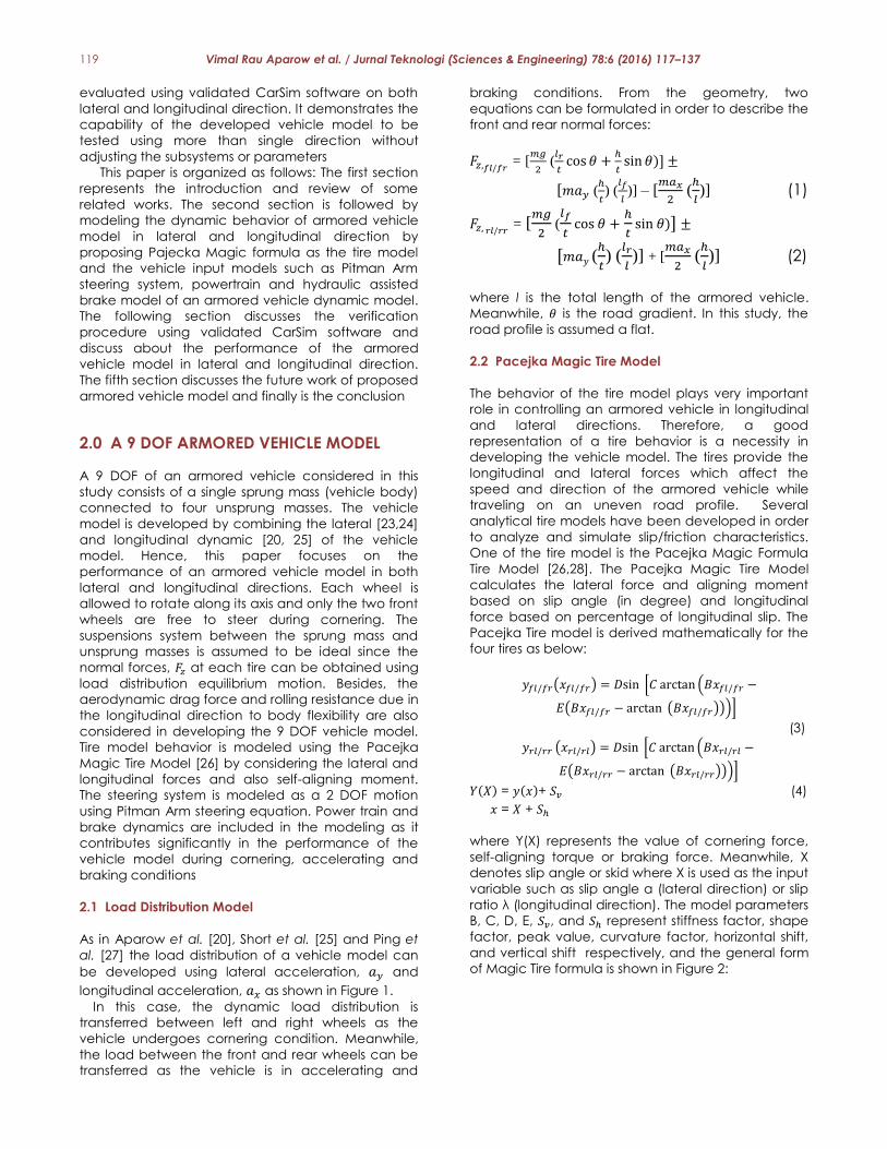
2.1 Load Distribution Model
As in Aparow et al. [20], Short et al. [25] and Ping et
al. [27] the load distribution of a vehicle model can
be developed using lateral acceleration, 𝑎𝑦 and
longitudinal acceleration, 𝑎𝑥 as shown in Figure 1.
In this case, the dynamic load distribution is
transferred between left and right wheels as the
vehicle undergoes cornering condition. Meanwhile,
the load between the front and rear wheels can be
transferred as the vehicle is in accelerating and
braking conditions. From the geometry, two
equations can be formulated in order to describe the
front and rear normal forces:
𝐹𝑧,𝑓𝑙/𝑓𝑟 = [
𝑚𝑔
2 (
𝑙𝑟
𝑡cos 𝜃 +
ℎ
𝑡sin 𝜃)] ±
[𝑚𝑎𝑦 (ℎ
𝑡) (
𝑙𝑓
𝑙)] – [
𝑚𝑎𝑥
2 (
ℎ
𝑙)] (1)
𝐹𝑧, 𝑟𝑙/𝑟𝑟 = [
𝑚𝑔
2 (
𝑙𝑓
𝑡cos 𝜃 +
ℎ
𝑡sin 𝜃)] ±
[𝑚𝑎𝑦 (ℎ
𝑡) (
𝑙𝑟
𝑙)] + [
𝑚𝑎𝑥
2 (
ℎ
𝑙)] (2)
where l is the total length of the armored vehicle.
Meanwhile, 𝜃 is the road gradient. In this study, the
road profile is assumed a flat.
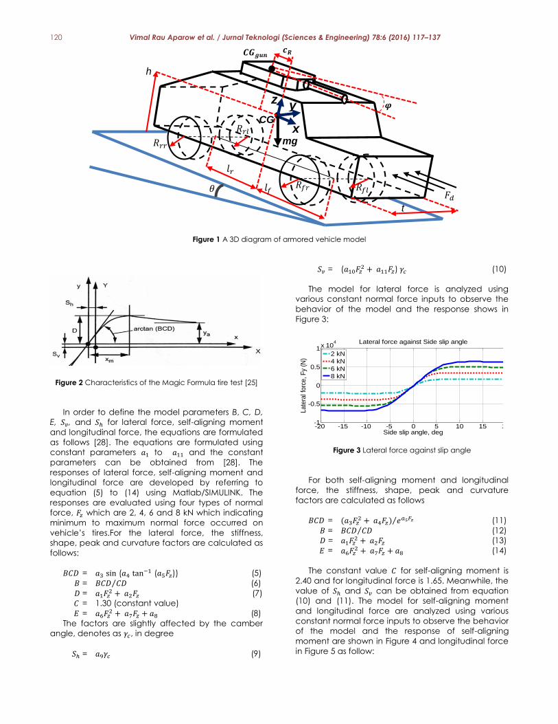
2.2 Pacejka Magic Tire Model
The behavior of the tire model plays very important
role in controlling an armored vehicle in longitudinal
and lateral directions. Therefore, a good
representation of a tire behavior is a necessity in
developing the vehicle model. The tires provide the
longitudinal and lateral forces which affect the
speed and direction of the armored vehicle while
traveling on an uneven road profile. Several
analytical tire models have been developed in order
to analyze and simulate slip/friction characteristics.
One of the tire model is the Pacejka Magic Formula
Tire Model [26,28]. The Pacejka Magic Tire Model
calculates the lateral force and aligning moment
based on slip angle (in degree) and longitudinal
force based on percentage of longitudinal slip. The
Pacejka Tire model is derived mathematically for the
four tires as below:
𝑦𝑓𝑙/𝑓𝑟(𝑥𝑓𝑙/𝑓𝑟) = 𝐷sin [𝐶 arctan (𝐵𝑥𝑓𝑙/𝑓𝑟 −
𝐸(𝐵𝑥𝑓𝑙/𝑓𝑟 − arctan (𝐵𝑥𝑓𝑙/𝑓𝑟)))]
(3)
𝑦𝑟𝑙/𝑟𝑟 (𝑥𝑟𝑙/𝑟𝑙) = 𝐷sin [𝐶 arctan (𝐵𝑥𝑟𝑙/𝑟𝑙 −
𝐸(𝐵𝑥𝑟𝑙/𝑟𝑟 − arctan (𝐵𝑥𝑟𝑙/𝑟𝑟)))]
𝑌(𝑋) = 𝑦(𝑥)+ 𝑆𝑣 (4)
𝑥 = 𝑋 + 𝑆ℎ
where Y(X) represents the value of cornering force,
self-aligning torque or braking force. Meanwhile, X
denotes slip angle or skid where X is used as the input
variable such as slip angle α (lateral direction) or slip
ratio λ (longitudinal direction). The model parameters
B, C, D, E, 𝑆𝑣, and 𝑆ℎ represent stiffness factor, shape
factor, peak value, curvature factor, horizontal shift,
and vertical shift respectively, and the general form
of Magic Tire formula is shown in Figure 2:
120 Vimal Rau Aparow et al. / Jurnal Teknologi (Sciences & Engineering) 78:6 (2016) 117–137
Figure 1 A 3D diagram of armored vehicle model
Figure 2 Characteristics of the Magic Formula tire test [25]
In order to define the model parameters B, C, D,
E, 𝑆𝑣, and 𝑆ℎ for lateral force, self-aligning moment
and longitudinal force, the equations are formulated
as follows [28]. The equations are formulated using
constant parameters 𝑎1 to 𝑎11 and the constant
parameters can be obtained from [28]. The
responses of lateral force, self-aligning moment and
longitudinal force are developed by referring to
equation (5) to (14) using Matlab/SIMULINK. The
responses are evaluated using four types of normal
force, 𝐹𝑧 which are 2, 4, 6 and 8 kN which indicating
minimum to maximum normal force occurred on
vehicle’s tires.For the lateral force, the stiffness,
shape, peak and curvature factors are calculated as
follows:
𝐵𝐶𝐷 = 𝑎3 sin (𝑎4 tan−1 (𝑎5𝐹𝑧)) (5)
𝐵 = 𝐵𝐶𝐷 𝐶𝐷⁄ (6)
𝐷 = 𝑎1𝐹𝑧2 + 𝑎2𝐹𝑧 (7)
𝐶 = 1.30 (constant value)
𝐸 = 𝑎6𝐹𝑧2 + 𝑎7𝐹𝑧 + 𝑎8 (8)
The factors are slightly affected by the camber
angle, denotes as 𝛾𝑐, in degree
𝑆ℎ = 𝑎9𝛾𝑐 (9)
𝑆𝑣 = (𝑎10𝐹𝑧2 + 𝑎11𝐹𝑧) 𝛾𝑐 (10)
The model for lateral force is analyzed using
various constant normal force inputs to observe the
behavior of the model and the response shows in
Figure 3:
Figure 3 Lateral force against slip angle
For both self-aligning moment and longitudinal
force, the stiffness, shape, peak and curvature
factors are calculated as follows
𝐵𝐶𝐷 = (𝑎3𝐹𝑧2 + 𝑎4𝐹𝑧) 𝑒𝑎5𝐹𝑧⁄ (11)
𝐵 = 𝐵𝐶𝐷 𝐶𝐷⁄ (12)
𝐷 = 𝑎1𝐹𝑧2 + 𝑎2𝐹𝑧 (13)
𝐸 = 𝑎6𝐹𝑧2 + 𝑎7𝐹𝑧 + 𝑎8 (14)
The constant value 𝐶 for self-aligning moment is
2.40 and for longitudinal force is 1.65. Meanwhile, the
value of 𝑆ℎ and 𝑆𝑣 can be obtained from equation
(10) and (11). The model for self-aligning moment
and longitudinal force are analyzed using various
constant normal force inputs to observe the behavior
of the model and the response of self-aligning
moment are shown in Figure 4 and longitudinal force
in Figure 5 as follow:
-20 -15 -10 -5 0 5 10 15 20-1
-0.5
0
0.5
1x 10
4
Side slip angle, deg
Late
ral f
orc
e, F
y (N
)
Lateral force against Side slip angle
2 kN
4 kN
6 kN
8 kN
𝑅𝑓𝑟
𝑅𝑟𝑟
𝑅𝑓𝑙
𝑅𝑟𝑙
𝑙𝑟
𝑙𝑓
h_
z_
x
y_
t_
𝜃_
CG
𝐹𝑑
mg__
𝑪𝑮𝒈𝒖𝒏 𝒄𝑹
𝝋
121 Vimal Rau Aparow et al. / Jurnal Teknologi (Sciences & Engineering) 78:6 (2016) 117–137
Figure 4 Self-aligning moment against slip angle
Figure 5 Longitudinal force against slip ratio
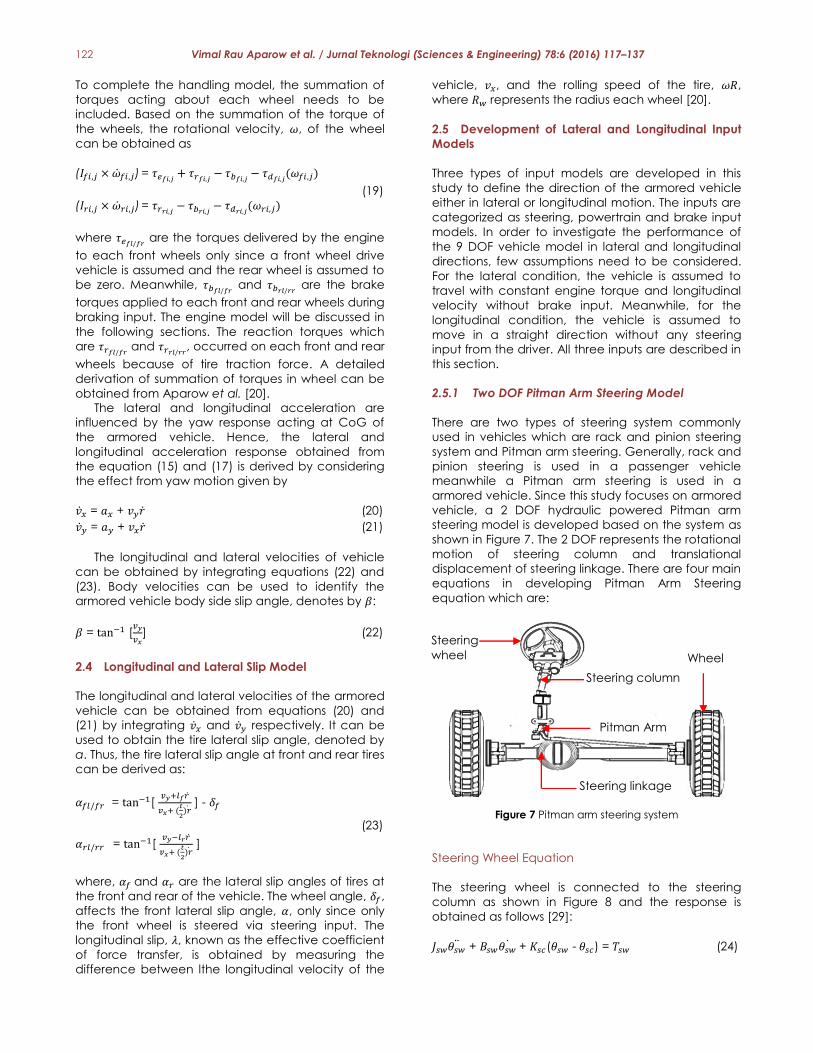
2.3 Handling Model
The handling model described in this paper is a 7
degrees of freedom system as shown in Figure 6. It
consists of 3 degrees of freedom of the armored
vehicle body in lateral and longitudinal motions as
well as yaw motion (r) and a single degree of
freedom due to the rotational motion of each tire.
The armored vehicle experiences motion along the
longitudinal x-axis, the lateral y-axis, and the angular
motions of yaw around the vertical z-axis. The motion
in the horizontal plane can be characterized by the
longitudinal and lateral accelerations, denoted by 𝑎𝑥
and 𝑎𝑦 respectively. In order to obtain the lateral
and longitudinal accelerations, summations of total
forces acting in lateral and longitudinal directions
are considered in this model. The total longitudinal
forces acting at the front and rear of the armored
vehicle is the sum of the normal, drag and recoil
force as
𝐹𝑥𝑡𝑜𝑡𝑎𝑙 = m𝑎𝑥
= 𝐹𝑥𝑟𝑟 + 𝐹𝑥𝑟𝑙 + 𝐹𝑦𝑓𝑟sin 𝛿𝑓 + 𝐹𝑦𝑓𝑙sin 𝛿𝑓 + 𝐹𝑥𝑓𝑟cos 𝛿𝑓
+ 𝐹𝑥𝑓𝑙cos 𝛿𝑓 + 𝑚𝑔 sin 𝜃 − 𝐹𝑑+ 𝐹𝑅cos 𝜑 (15)
The 𝐹𝑅 is the recoil force due to gun firing. The
drag force, 𝐹𝑑 , is an important in the model which is
used to limit the maximum linear speed of a vehicle
in the longitudinal direction. The drag force can be
derived by summing the aerodynamic resistance
force, 𝐹𝑎 and rolling resistance force, 𝐹𝑟 as shown
below:
𝐹𝑑 = 𝐹𝑎 + 𝐹𝑟 = 1
2 𝜌𝐴𝐶𝑑(𝑣𝑥
2) + 𝑚𝑔𝐶𝑟(𝑣𝑥) (16)
Since the armored vehicle model is developed
based on both lateral and longitudinal dynamics,
hence the equation related to drag force acting in
the longitudinal direction is summed as the total of
forces acting in the longitudinal direction in order to
obtain longitudinal acceleration, 𝑎𝑥. Meanwhile, the
total force acting in the lateral direction is
𝐹𝑦𝑡𝑜𝑡𝑎𝑙 = m𝑎𝑦
= 𝐹𝑦𝑟𝑟 + 𝐹𝑦𝑟𝑙 + 𝐹𝑦𝑓𝑟cos 𝛿𝑓 + 𝐹𝑦𝑓𝑙cos 𝛿𝑓 – 𝐹𝑥𝑓𝑟sin 𝛿𝑓 -
𝐹𝑥𝑓𝑙sin 𝛿𝑓 - 𝐹𝑅sin 𝜑
(17)
The yaw acceleration, �̈�, is also dependent on the
longitudinal and lateral forces, 𝐹𝑥 and 𝐹𝑦 which are
acting on each of the front and rear tires. Besides,
the self-aligning moment from each tires are also
considered in deriving the total yaw moment acting
at CG of the vehicle, thus
𝑀𝑦𝑎𝑤 = 𝐼𝑦𝑎𝑤�̈�
= [𝐹𝑥𝑟𝑟 - 𝐹𝑥𝑟𝑙 - 𝐹𝑦𝑓𝑟sin 𝛿𝑓 + 𝐹𝑦𝑓𝑙sin 𝛿𝑓 – 𝐹𝑥𝑓𝑟cos 𝛿𝑓 +
𝐹𝑥𝑓𝑙cos 𝛿𝑓] t/2 + [𝐹𝑦𝑟𝑟 + 𝐹𝑦𝑟𝑙]𝑙𝑟 + [- 𝐹𝑦𝑓𝑟cos 𝛿𝑓 -
𝐹𝑦𝑓𝑙cos 𝛿𝑓 + 𝐹𝑥𝑓𝑟sin 𝛿𝑓 + 𝐹𝑥𝑓𝑙sin 𝛿𝑓]𝑙𝑓 + 𝑀𝑧𝑓𝑙+
𝑀𝑧𝑓𝑟+ 𝑀𝑧𝑟𝑙
+ 𝑀𝑧𝑟𝑟 + [(𝐹𝑅sin 𝜑) × 𝑐𝑅] (18)
-20 -15 -10 -5 0 5 10 15 20-200
-100
0
100
200
Side slip angle, deg
Self
Alig
nin
g M
om
ent, M
z (N
m) Self Aligning Moment against Side Slip angle
8 kN
6 kN
4 kN
2 kN
0 20 40 60 80 1000
2000
4000
6000
8000
Longitudinal slip, %
Bra
ke forc
e, F
x (
N)
Brake force against longitudinal slip
2 kN
4 kN
6 kN
8 kN
Figure 6 A 7 DOF handling model
𝐹𝑥𝑟𝑙
𝐹𝑦𝑟𝑙
𝐹𝑦𝑟𝑟
𝐹𝑥𝑟𝑟
w_
𝑙𝑟
𝐹𝑦𝑓𝑙
𝐹𝑥𝑓𝑙
𝐹𝑦𝑓𝑟
𝐹𝑥𝑓𝑟
𝛿𝑓
𝛿𝑓
𝐹𝑑
𝐹𝑅
𝑣𝑦
𝑣𝑥
v_ 𝛽
𝜑
𝑐𝑅
r
𝑙𝑓
CG
122 Vimal Rau Aparow et al. / Jurnal Teknologi (Sciences & Engineering) 78:6 (2016) 117–137
To complete the handling model, the summation of
torques acting about each wheel needs to be
included. Based on the summation of the torque of
the wheels, the rotational velocity, 𝜔, of the wheel
can be obtained as
(𝐼𝑓𝑖,𝑗 × �̇�𝑓𝑖,𝑗) = 𝜏𝑒𝑓𝑖,𝑗+ 𝜏𝑟𝑓𝑖,𝑗
− 𝜏𝑏𝑓𝑖,𝑗− 𝜏𝑑𝑓𝑖,𝑗
(𝜔𝑓𝑖,𝑗)
(19)
(𝐼𝑟𝑖,𝑗 × �̇�𝑟𝑖,𝑗) = 𝜏𝑟𝑟𝑖,𝑗− 𝜏𝑏𝑟𝑖,𝑗
− 𝜏𝑑𝑟𝑖,𝑗(𝜔𝑟𝑖,𝑗)
where 𝜏𝑒𝑓𝑙/𝑓𝑟 are the torques delivered by the engine
to each front wheels only since a front wheel drive
vehicle is assumed and the rear wheel is assumed to
be zero. Meanwhile, 𝜏𝑏𝑓𝑙/𝑓𝑟 and 𝜏𝑏𝑟𝑙/𝑟𝑟
are the brake
torques applied to each front and rear wheels during
braking input. The engine model will be discussed in
the following sections. The reaction torques which
are 𝜏𝑟𝑓𝑙/𝑓𝑟 and 𝜏𝑟𝑟𝑙/𝑟𝑟
, occurred on each front and rear
wheels because of tire traction force. A detailed
derivation of summation of torques in wheel can be
obtained from Aparow et al. [20].
The lateral and longitudinal acceleration are
influenced by the yaw response acting at CoG of
the armored vehicle. Hence, the lateral and
longitudinal acceleration response obtained from
the equation (15) and (17) is derived by considering
the effect from yaw motion given by
�̇�𝑥 = 𝑎𝑥 + 𝑣𝑦�̇� (20)
�̇�𝑦 = 𝑎𝑦 + 𝑣𝑥�̇� (21)
The longitudinal and lateral velocities of vehicle
can be obtained by integrating equations (22) and
(23). Body velocities can be used to identify the
armored vehicle body side slip angle, denotes by 𝛽:
𝛽 = tan−1 [𝑣𝑦
𝑣𝑥] (22)
2.4 Longitudinal and Lateral Slip Model
The longitudinal and lateral velocities of the armored
vehicle can be obtained from equations (20) and
(21) by integrating �̇�𝑥 and �̇�𝑦 respectively. It can be
used to obtain the tire lateral slip angle, denoted by
α. Thus, the tire lateral slip angle at front and rear tires
can be derived as:
𝛼𝑓𝑙/𝑓𝑟 = tan−1[ 𝑣𝑦+𝑙𝑓�̇�
𝑣𝑥+ (𝑡
2)�̇�
] - 𝛿𝑓
(23)
𝛼𝑟𝑙/𝑟𝑟 = tan−1[ 𝑣𝑦−𝑙𝑟�̇�
𝑣𝑥+ (𝑡
2)�̇�
]
where, 𝛼𝑓 and 𝛼𝑟 are the lateral slip angles of tires at
the front and rear of the vehicle. The wheel angle, 𝛿𝑓,
affects the front lateral slip angle, 𝛼, only since only
the front wheel is steered via steering input. The
longitudinal slip, 𝜆, known as the effective coefficient
of force transfer, is obtained by measuring the
difference between lthe longitudinal velocity of the
vehicle, 𝑣𝑥, and the rolling speed of the tire, 𝜔𝑅,
where 𝑅𝑤 represents the radius each wheel [20].
2.5 Development of Lateral and Longitudinal Input
Models
Three types of input models are developed in this
study to define the direction of the armored vehicle
either in lateral or longitudinal motion. The inputs are
categorized as steering, powertrain and brake input
models. In order to investigate the performance of
the 9 DOF vehicle model in lateral and longitudinal
directions, few assumptions need to be considered.
For the lateral condition, the vehicle is assumed to
travel with constant engine torque and longitudinal
velocity without brake input. Meanwhile, for the
longitudinal condition, the vehicle is assumed to
move in a straight direction without any steering
input from the driver. All three inputs are described in
this section.
2.5.1 Two DOF Pitman Arm Steering Model
There are two types of steering system commonly
used in vehicles which are rack and pinion steering
system and Pitman arm steering. Generally, rack and
pinion steering is used in a passenger vehicle
meanwhile a Pitman arm steering is used in a
armored vehicle. Since this study focuses on armored
vehicle, a 2 DOF hydraulic powered Pitman arm
steering model is developed based on the system as
shown in Figure 7. The 2 DOF represents the rotational
motion of steering column and translational
displacement of steering linkage. There are four main
equations in developing Pitman Arm Steering
equation which are:
Figure 7 Pitman arm steering system
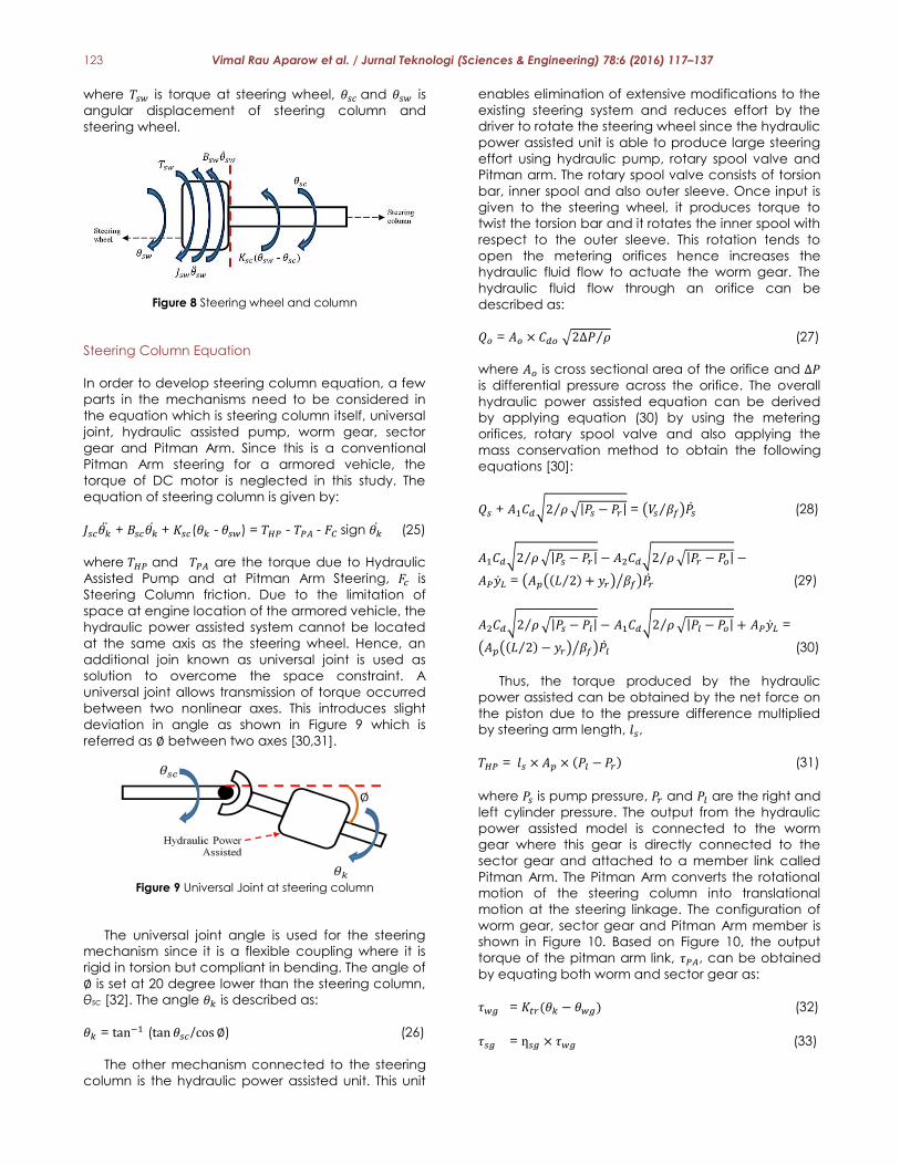
Steering Wheel Equation
The steering wheel is connected to the steering
column as shown in Figure 8 and the response is
obtained as follows [29]:
𝐽𝑠𝑤𝜃𝑠�̈� + 𝐵𝑠𝑤𝜃𝑠�̇� + 𝐾𝑠𝑐(𝜃𝑠𝑤 - 𝜃𝑠𝑐) = 𝑇𝑠𝑤 (24)
Steering
wheel Wheel
Steering column
Pitman Arm
Steering linkage
123 Vimal Rau Aparow et al. / Jurnal Teknologi (Sciences & Engineering) 78:6 (2016) 117–137
where 𝑇𝑠𝑤 is torque at steering wheel, 𝜃𝑠𝑐 and 𝜃𝑠𝑤 is
angular displacement of steering column and
steering wheel.
Figure 8 Steering wheel and column
Steering Column Equation
In order to develop steering column equation, a few
parts in the mechanisms need to be considered in
the equation which is steering column itself, universal
joint, hydraulic assisted pump, worm gear, sector
gear and Pitman Arm. Since this is a conventional
Pitman Arm steering for a armored vehicle, the
torque of DC motor is neglected in this study. The
equation of steering column is given by:
𝐽𝑠𝑐𝜃�̈� + 𝐵𝑠𝑐𝜃�̇� + 𝐾𝑠𝑐(𝜃𝑘 - 𝜃𝑠𝑤) = 𝑇𝐻𝑃 - 𝑇𝑃𝐴 - 𝐹𝐶 sign 𝜃�̇� (25)
where 𝑇𝐻𝑃 and 𝑇𝑃𝐴 are the torque due to Hydraulic
Assisted Pump and at Pitman Arm Steering, 𝐹𝑐 is
Steering Column friction. Due to the limitation of
space at engine location of the armored vehicle, the
hydraulic power assisted system cannot be located
at the same axis as the steering wheel. Hence, an
additional join known as universal joint is used as
solution to overcome the space constraint. A
universal joint allows transmission of torque occurred
between two nonlinear axes. This introduces slight
deviation in angle as shown in Figure 9 which is
referred as ∅ between two axes [30,31].
Figure 9 Universal Joint at steering column
The universal joint angle is used for the steering
mechanism since it is a flexible coupling where it is
rigid in torsion but compliant in bending. The angle of
∅ is set at 20 degree lower than the steering column,
θsc [32]. The angle 𝜃𝑘 is described as:
𝜃𝑘 = tan−1 (tan 𝜃𝑠𝑐/cos ∅) (26)
The other mechanism connected to the steering
column is the hydraulic power assisted unit. This unit
enables elimination of extensive modifications to the
existing steering system and reduces effort by the
driver to rotate the steering wheel since the hydraulic
power assisted unit is able to produce large steering
effort using hydraulic pump, rotary spool valve and
Pitman arm. The rotary spool valve consists of torsion
bar, inner spool and also outer sleeve. Once input is
given to the steering wheel, it produces torque to
twist the torsion bar and it rotates the inner spool with
respect to the outer sleeve. This rotation tends to
open the metering orifices hence increases the
hydraulic fluid flow to actuate the worm gear. The
hydraulic fluid flow through an orifice can be
described as:
𝑄𝑜 = 𝐴𝑜 × 𝐶𝑑𝑜 √2∆𝑃 𝜌⁄ (27)
where 𝐴𝑜 is cross sectional area of the orifice and ∆𝑃
is differential pressure across the orifice. The overall
hydraulic power assisted equation can be derived
by applying equation (30) by using the metering
orifices, rotary spool valve and also applying the
mass conservation method to obtain the following
equations [30]:
𝑄𝑠 + 𝐴1𝐶𝑑√2 𝜌⁄ √|𝑃𝑠 − 𝑃𝑟| = (𝑉𝑠 𝛽𝑓⁄ )𝑃�̇� (28)
𝐴1𝐶𝑑√2 𝜌⁄ √|𝑃𝑠 − 𝑃𝑟| − 𝐴2𝐶𝑑√2 𝜌⁄ √|𝑃𝑟 − 𝑃𝑜| −
𝐴𝑃�̇�𝐿 = (𝐴𝑝((𝐿 2⁄ ) + 𝑦𝑟) 𝛽𝑓⁄ )𝑃�̇� (29)
𝐴2𝐶𝑑√2 𝜌⁄ √|𝑃𝑠 − 𝑃𝑙| − 𝐴1𝐶𝑑√2 𝜌⁄ √|𝑃𝑙 − 𝑃𝑜| + 𝐴𝑃�̇�𝐿 =
(𝐴𝑝((𝐿 2⁄ ) − 𝑦𝑟) 𝛽𝑓⁄ )𝑃�̇� (30)
Thus, the torque produced by the hydraulic
power assisted can be obtained by the net force on
the piston due to the pressure difference multiplied
by steering arm length, 𝑙𝑠,
𝑇𝐻𝑃 = 𝑙𝑠 × 𝐴𝑝 × (𝑃𝑙 − 𝑃𝑟) (31)
where 𝑃𝑠 is pump pressure, 𝑃𝑟 and 𝑃𝑙 are the right and
left cylinder pressure. The output from the hydraulic
power assisted model is connected to the worm
gear where this gear is directly connected to the
sector gear and attached to a member link called
Pitman Arm. The Pitman Arm converts the rotational
motion of the steering column into translational
motion at the steering linkage. The configuration of
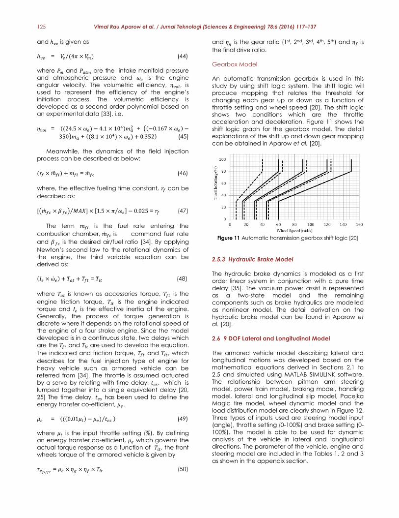
worm gear, sector gear and Pitman Arm member is
shown in Figure 10. Based on Figure 10, the output
torque of the pitman arm link, 𝜏𝑃𝐴, can be obtained
by equating both worm and sector gear as:
𝜏𝑤𝑔 = 𝐾𝑡𝑟(𝜃𝑘 − 𝜃𝑤𝑔) (32)
𝜏𝑠𝑔 = ƞ𝑠𝑔 × 𝜏𝑤𝑔 (33)
124 Vimal Rau Aparow et al. / Jurnal Teknologi (Sciences & Engineering) 78:6 (2016) 117–137
Since the torque created at sector gear is equal to
the torque created at the end joint of pitman arm,
Figure 10 Mechanical configuration between worm gear,
sector gear and pitman arm
𝜏𝑠𝑔 = 𝜏𝑃𝐴 (34)
where 𝜏𝑠𝑔, 𝜏𝑤𝑔 and 𝜏𝑃𝐴 are the torques at sector
gear, worm gear and at pitman arm joint.
Steering Linkage Equation
The rotational input from the sector gear is converted
into translational motion to the steering linkage using
Pitman Arm joint link. By using the torque from Pitman
Arm as the input torque, the equation of motion of
the steering linkage is [29]:
𝑀𝐿𝑦�̈� + 𝐵𝐿𝑦�̇� + [𝐶𝑆𝐿 sgn (𝑦�̇�)] – [ 𝑏𝑟×𝑇𝑃𝐴
𝑀𝐿×𝑅𝑃𝐴 ]
= ƞ𝑓(𝑇𝑃𝐴
𝑅𝑃𝐴) – ƞ𝐵(
𝑇𝐾𝐿
𝑁𝑀) (35)
and torque at steering linkage, 𝑇𝐾𝐿 is
𝑇𝐾𝐿 = 𝐾𝑆𝐿 (𝑦𝐿
𝑁𝑀− 𝛿𝑓) (36)
where 𝑀𝐿 is the Mass of steering linkage of Pitman
Arm Steering, 𝐵𝐿 and 𝑦𝐿 are viscous damping and
translational displacement of steering linkage and 𝑏𝑟
is resistance occurred on steering linkage. 𝑅𝑃𝐴 is
radius of Pitman Arm and 𝑁𝑀 is the motor gearbox
ratio.
Equation of Motion of Wheel
Using equations (24), (25), (31) and (35), equation of
motion of the wheel can be obtained. The output
response of wheel equation of motion, known as
wheel angle, 𝛿𝑓, is given by
𝐽𝑓𝑤𝛿�̈� + 𝐵𝑓𝑤𝛿�̇� + [𝐶𝑓𝑤sign (𝛿�̇�)] = 𝑇𝐾𝐿+ 𝑇𝑒𝑥𝑡 + 𝑇𝑎 (37)
where 𝐽𝑓𝑤 is moment of Inertia of wheel, 𝐵𝑓𝑤 is
viscous damping of steering linkage bushing, 𝐶𝐹𝑊 is
coulomb friction breakout force on road front wheel,
𝑇𝑒𝑥𝑡 is external torque due to road wheel and 𝑇𝑎 is
tire alignment moment from Pacejka Magic Tire
model. The front wheel angle, 𝛿𝑓, obtained from the
2 DOF Pitman arm steering model is used in
equations (15), (17), (18) and (23).
2.5.1 Power Train Model
The powertrain model is one of the important
subsystems in the vehicle model to generate engine
torque in order to produce rotational motion to the
front wheels. The model consists of internal engine
dynamics, gearbox and final drive differential model.
These models are used to transfer the engine torque
to the front wheels once the vehicle starts to
accelerate, cornering or braking [20, 25].
Engine Dynamics
The engine dynamics have been developed based
on Moskwa and Hedrick [33] which focuses on
automotive engine meanwhile Wahlström and
Eriksson [34] focused on diesel type of engine. The
equations developed are more focused with three
variables which are mass of air intake manifold,
engine speed, mass flow rate of fuel entering
combustion chamber and the output torque. By
applying the law of conservation of mass to the air
flow in the intake manifold, the following equation
can be obtained:
�̇�𝑎 = �̇�𝑎𝑖 − �̇�𝑎𝑜 (38)
and
�̇�𝑎𝑖 = 𝑀𝐴𝑋 × 𝑇𝐶 × 𝑃𝑅𝐼 (39)
where 𝑚𝑎 is mass of air in the intake manifold,
𝑚𝑎̇ , �̇�𝑎𝑖, are the mass rate of air in the intake
manifold, mass rate of air entering the intake
manifold. �̇�𝑎𝑜 is leaving the intake manifold and
entering the combustion chamber. Meanwhile, 𝑇𝐶 is
the normalized throttle characteristic and 𝑃𝑅𝐼 is. The
term 𝑇𝐶 can be determined based on experimental
data as shown by Moskwa and Hedrick [33]. The
data is described as below:
𝑇𝐶 ={
where 𝛼𝑡 is the throttle angle of the opening throttle
body valve. Meanwhile, the normalized pressure
influence function, PRI, is the normalized pressure
influence function and measured as a ratio of
function manifold to atmospheric pressure:
𝑃𝑅𝐼 = 1 − exp [(𝑃𝑚 𝑃𝑎𝑡𝑚⁄ ) − 1] (41)
The mass of air and also the intake manifold
pressure enters the intake manifold is described using
ideal gas law which is:
𝑚𝑎 = ((𝑀𝑎 × 𝑃𝑚 × 𝑉𝑚) (𝑅 × 𝑇𝑚)⁄ ) (42)
Besides that, the flowing air from intake manifold
to the combustion chamber is given by
�̇�𝑎𝑜 = ℎ𝑣𝑒 × 𝜔𝑒 × 𝜂𝑣𝑜𝑙 × 𝑚𝑎 (43)
1 − cos[(1.14459 × 𝛼𝑡) − 1.06]; 𝛼𝑡 ≤ 79.5
1 𝛼𝑡 > 79.6 (40)
125 Vimal Rau Aparow et al. / Jurnal Teknologi (Sciences & Engineering) 78:6 (2016) 117–137
and ℎ𝑣𝑒 is given as
ℎ𝑣𝑒 = 𝑉𝑒 (4𝜋⁄ × 𝑉𝑚) (44)
where 𝑃𝑚 and 𝑃𝑎𝑡𝑚 are the intake manifold pressure
and atmospheric pressure and 𝜔𝑒 is the engine
angular velocity. The volumetric efficiency, 𝜂𝑣𝑜𝑙, is
used to represent the efficiency of the engine’s
initiation process. The volumetric efficiency is
developed as a second order polynomial based on
an experimental data [33], i.e.
𝜂𝑣𝑜𝑙 = ((24.5 × 𝜔𝑒) − 4.1 × 10⁴)𝑚𝑎2 + ((−0.167 × 𝜔𝑒) −
350)𝑚𝑎 + ((8.1 × 10⁴) × 𝜔𝑒) + 0.352) (45)
Meanwhile, the dynamics of the field injection
process can be described as below:
(𝑟𝑓 × �̈�𝑓𝑖) + 𝑚𝑓𝑖 = �̇�𝑓𝑐 (46)
where, the effective fueling time constant, 𝑟𝑓 can be
described as:
[(�̇�𝑓𝑐 × 𝛽 𝑓𝑐) 𝑀𝐴𝑋]⁄ × [1.5 × 𝜋 𝜔𝑒⁄ ] − 0.025 = 𝑟𝑓 (47)
The term 𝑚𝑓𝑖 is the fuel rate entering the
combustion chamber, �̇�𝑓𝑐 is command fuel rate
and 𝛽 𝑓𝑐 is the desired air/fuel ratio [34]. By applying
Newton’s second law to the rotational dynamics of
the engine, the third variable equation can be
derived as:
(𝐼𝑒 × �̇�𝑒) + 𝑇𝑎𝑡 + 𝑇𝑓𝑡 = 𝑇𝑖𝑡 (48)
where 𝑇𝑎𝑡 is known as accessories torque, 𝑇𝑓𝑡 is the
engine friction torque, 𝑇𝑖𝑡 is the engine indicated
torque and 𝐼𝑒 is the effective inertia of the engine.
Generally, the process of torque generation is
discrete where it depends on the rotational speed of
the engine of a four stroke engine. Since the model
developed is in a continuous state, two delays which
are the 𝑇𝑓𝑡 and 𝑇𝑖𝑡 are used to develop the equation.
The indicated and friction torque, 𝑇𝑓𝑡 and 𝑇𝑖𝑡, which
describes for the fuel injection type of engine for
heavy vehicle such as armored vehicle can be
referred from [34]. The throttle is assumed actuated
by a servo by relating with time delay, 𝑡𝑒𝑠, which is
lumped together into a single equivalent delay [20,
25] The time delay, 𝑡𝑒𝑠 has been used to define the
energy transfer co-efficient, 𝜇𝑒.
�̇�𝑒 = (((0.01𝜇𝑡) − 𝜇𝑒) 𝑡𝑒𝑠 ⁄ ) (49)
where 𝜇𝑡 is the input throttle setting (%). By defining
an energy transfer co-efficient, 𝜇𝑒 which governs the
actual torque response as a function of 𝑇𝑖𝑡, the front
wheels torque of the armored vehicle is given by
𝜏𝑒𝑓𝑙/𝑓𝑟 = 𝜇𝑒 × 𝜂𝑔 × 𝜂𝑓 × 𝑇𝑖𝑡 (50)
and 𝜂𝑔 is the gear ratio (1st, 2nd, 3rd, 4th, 5th) and 𝜂𝑓 is
the final drive ratio.
Gearbox Model
An automatic transmission gearbox is used in this
study by using shift logic system. The shift logic will
produce mapping that relates the threshold for
changing each gear up or down as a function of
throttle setting and wheel speed [20]. The shift logic
shows two conditions which are the throttle
acceleration and deceleration. Figure 11 shows the
shift logic graph for the gearbox model. The detail
explanations of the shift up and down gear mapping
can be obtained in Aparow et al. [20].
Figure 11 Automatic transmission gearbox shift logic [20]
2.5.3 Hydraulic Brake Model
The hydraulic brake dynamics is modeled as a first
order linear system in conjunction with a pure time
delay [35]. The vacuum power assist is represented
as a two-state model and the remaining
components such as brake hydraulics are modelled
as nonlinear model. The detail derivation on the
hydraulic brake model can be found in Aparow et
al. [20].
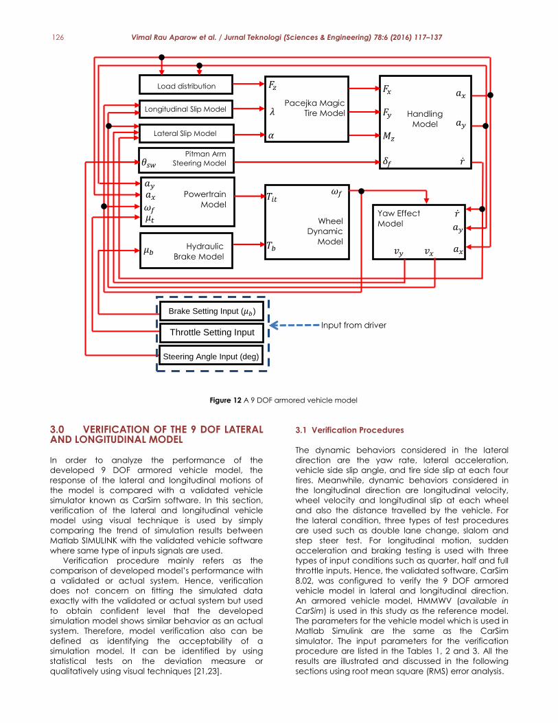
2.6 9 DOF Lateral and Longitudinal Model
The armored vehicle model describing lateral and
longitudinal motions was developed based on the
mathematical equations derived in Sections 2.1 to
2.5 and simulated using MATLAB SIMULINK software.
The relationship between pitman arm steering
model, power train model, braking model, handling
model, lateral and longitudinal slip model, Pacejka
Magic tire model, wheel dynamic model and the
load distribution model are clearly shown in Figure 12.
Three types of inputs used are steering model input
(angle), throttle setting (0-100%) and brake setting (0-
100%). The model is able to be used for dynamic
analysis of the vehicle in lateral and longitudinal
directions. The parameter of the vehicle, engine and
steering model are included in the Tables 1, 2 and 3
as shown in the appendix section.
126 Vimal Rau Aparow et al. / Jurnal Teknologi (Sciences & Engineering) 78:6 (2016) 117–137
Figure 12 A 9 DOF armored vehicle model
3.0 VERIFICATION OF THE 9 DOF LATERAL AND LONGITUDINAL MODEL
In order to analyze the performance of the
developed 9 DOF armored vehicle model, the
response of the lateral and longitudinal motions of
the model is compared with a validated vehicle
simulator known as CarSim software. In this section,
verification of the lateral and longitudinal vehicle
model using visual technique is used by simply
comparing the trend of simulation results between
Matlab SIMULINK with the validated vehicle software
where same type of inputs signals are used.
Verification procedure mainly refers as the
comparison of developed model’s performance with
a validated or actual system. Hence, verification
does not concern on fitting the simulated data
exactly with the validated or actual system but used
to obtain confident level that the developed
simulation model shows similar behavior as an actual
system. Therefore, model verification also can be
defined as identifying the acceptability of a
simulation model. It can be identified by using
statistical tests on the deviation measure or
qualitatively using visual techniques [21,23].
3.1 Verification Procedures
The dynamic behaviors considered in the lateral
direction are the yaw rate, lateral acceleration,
vehicle side slip angle, and tire side slip at each four
tires. Meanwhile, dynamic behaviors considered in
the longitudinal direction are longitudinal velocity,
wheel velocity and longitudinal slip at each wheel
and also the distance travelled by the vehicle. For
the lateral condition, three types of test procedures
are used such as double lane change, slalom and
step steer test. For longitudinal motion, sudden
acceleration and braking testing is used with three
types of input conditions such as quarter, half and full
throttle inputs. Hence, the validated software, CarSim
8.02, was configured to verify the 9 DOF armored
vehicle model in lateral and longitudinal direction.
An armored vehicle model, HMMWV (available in
CarSim) is used in this study as the reference model.
The parameters for the vehicle model which is used in
Matlab Simulink are the same as the CarSim
simulator. The input parameters for the verification
procedure are listed in the Tables 1, 2 and 3. All the
results are illustrated and discussed in the following
sections using root mean square (RMS) error analysis.
𝜃𝑠𝑤
𝐹𝑧
𝜆
𝛼
𝜔𝑓 𝑇𝑖𝑡
𝑇𝑏
𝐹𝑥
𝐹𝑦
𝑀𝑧
𝛿𝑓
𝑎𝑥
𝑎𝑦
�̇�
Input from driver
�̇�
𝑎𝑦
𝑎𝑥 𝑣𝑦 𝑣𝑥
𝜔𝑓
Pitman Arm
Steering Model
Load distribution
model
Longitudinal Slip Model
Lateral Slip Model
Powertrain
Model
Pacejka Magic
Tire Model
Hydraulic
Brake Model
Handling
Model
Yaw Effect
Model Wheel
Dynamic
Model
Brake Setting Input (𝜇𝑏)
Throttle Setting Input
(𝜇𝑡)
Steering Angle Input (deg)
𝑎𝑥 𝑎𝑦
𝜇𝑡
𝜇𝑏
127 Vimal Rau Aparow et al. / Jurnal Teknologi (Sciences & Engineering) 78:6 (2016) 117–137
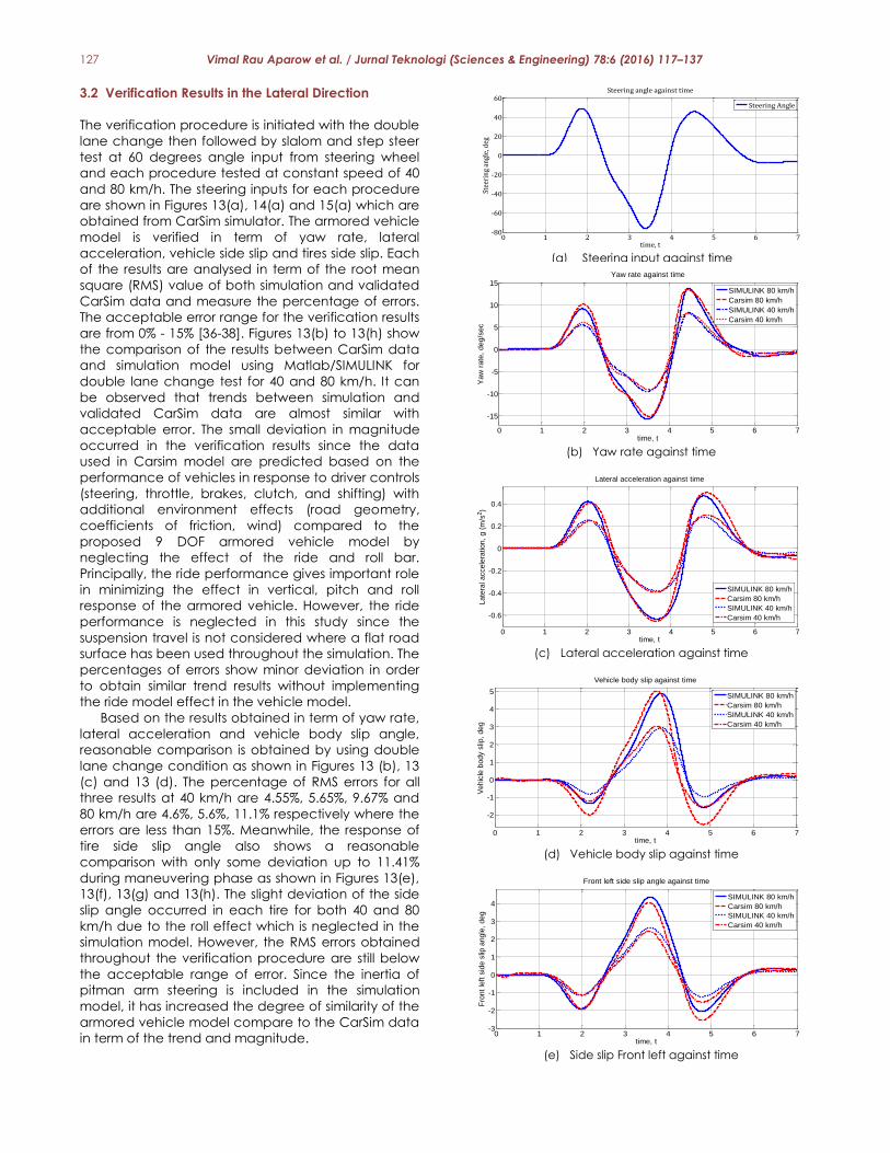
3.2 Verification Results in the Lateral Direction
The verification procedure is initiated with the double
lane change then followed by slalom and step steer
test at 60 degrees angle input from steering wheel
and each procedure tested at constant speed of 40
and 80 km/h. The steering inputs for each procedure
are shown in Figures 13(a), 14(a) and 15(a) which are
obtained from CarSim simulator. The armored vehicle
model is verified in term of yaw rate, lateral
acceleration, vehicle side slip and tires side slip. Each
of the results are analysed in term of the root mean
square (RMS) value of both simulation and validated
CarSim data and measure the percentage of errors.
The acceptable error range for the verification results
are from 0% - 15% [36-38]. Figures 13(b) to 13(h) show
the comparison of the results between CarSim data
and simulation model using Matlab/SIMULINK for
double lane change test for 40 and 80 km/h. It can
be observed that trends between simulation and
validated CarSim data are almost similar with
acceptable error. The small deviation in magnitude
occurred in the verification results since the data
used in Carsim model are predicted based on the
performance of vehicles in response to driver controls
(steering, throttle, brakes, clutch, and shifting) with
additional environment effects (road geometry,
coefficients of friction, wind) compared to the
proposed 9 DOF armored vehicle model by
neglecting the effect of the ride and roll bar.
Principally, the ride performance gives important role
in minimizing the effect in vertical, pitch and roll
response of the armored vehicle. However, the ride
performance is neglected in this study since the
suspension travel is not considered where a flat road
surface has been used throughout the simulation. The
percentages of errors show minor deviation in order
to obtain similar trend results without implementing
the ride model effect in the vehicle model.
Based on the results obtained in term of yaw rate,
lateral acceleration and vehicle body slip angle,
reasonable comparison is obtained by using double
lane change condition as shown in Figures 13 (b), 13
(c) and 13 (d). The percentage of RMS errors for all
three results at 40 km/h are 4.55%, 5.65%, 9.67% and
80 km/h are 4.6%, 5.6%, 11.1% respectively where the
errors are less than 15%. Meanwhile, the response of
tire side slip angle also shows a reasonable
comparison with only some deviation up to 11.41%
during maneuvering phase as shown in Figures 13(e),
13(f), 13(g) and 13(h). The slight deviation of the side
slip angle occurred in each tire for both 40 and 80
km/h due to the roll effect which is neglected in the
simulation model. However, the RMS errors obtained
throughout the verification procedure are still below
the acceptable range of error. Since the inertia of
pitman arm steering is included in the simulation
model, it has increased the degree of similarity of the
armored vehicle model compare to the CarSim data
in term of the trend and magnitude.
(a) Steering input against time
0 1 2 3 4 5 6 7-80
-60
-40
-20
0
20
40
60
time, t
Stee
rin
g an
gle,
deg
Steering angle against time
Steering Angle
(b) Yaw rate against time
(c) Lateral acceleration against time
(d) Vehicle body slip against time
(e) Side slip Front left against time
0 1 2 3 4 5 6 7
-15
-10
-5
0
5
10
15
time, t
Yaw
rate
, deg/s
ec
Yaw rate against time
SIMULINK 80 km/h
Carsim 80 km/h
SIMULINK 40 km/h
Carsim 40 km/h
0 1 2 3 4 5 6 7
-0.6
-0.4
-0.2
0
0.2
0.4
Lateral acceleration against time
time, t
La
tera
l a
cce
lera
tio
n,
g (
m/s
2)
SIMULINK 80 km/h
Carsim 80 km/h
SIMULINK 40 km/h
Carsim 40 km/h
0 1 2 3 4 5 6 7
-2
-1
0
1
2
3
4
5
time, t
Ve
hic
le b
ody s
lip,
de
g
Vehicle body slip against time
SIMULINK 80 km/h
Carsim 80 km/h
SIMULINK 40 km/h
Carsim 40 km/h
0 1 2 3 4 5 6 7-3
-2
-1
0
1
2
3
4
time, t
Fro
nt
left
sid
e s
lip a
ngle
, d
eg
Front left side slip angle against time
SIMULINK 80 km/h
Carsim 80 km/h
SIMULINK 40 km/h
Carsim 40 km/h
128 Vimal Rau Aparow et al. / Jurnal Teknologi (Sciences & Engineering) 78:6 (2016) 117–137
Figure 13 Response of the armored vehicle for double lane
change test at 40 and 80 km/h
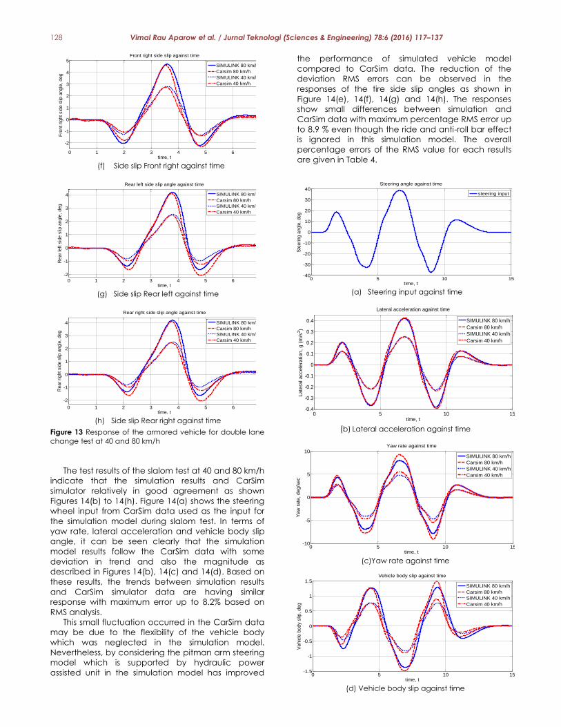
The test results of the slalom test at 40 and 80 km/h
indicate that the simulation results and CarSim
simulator relatively in good agreement as shown
Figures 14(b) to 14(h). Figure 14(a) shows the steering
wheel input from CarSim data used as the input for
the simulation model during slalom test. In terms of
yaw rate, lateral acceleration and vehicle body slip
angle, it can be seen clearly that the simulation
model results follow the CarSim data with some
deviation in trend and also the magnitude as
described in Figures 14(b), 14(c) and 14(d). Based on
these results, the trends between simulation results
and CarSim simulator data are having similar
response with maximum error up to 8.2% based on
RMS analysis.
This small fluctuation occurred in the CarSim data
may be due to the flexibility of the vehicle body
which was neglected in the simulation model.
Nevertheless, by considering the pitman arm steering
model which is supported by hydraulic power
assisted unit in the simulation model has improved
the performance of simulated vehicle model
compared to CarSim data. The reduction of the
deviation RMS errors can be observed in the
responses of the tire side slip angles as shown in
Figure 14(e), 14(f), 14(g) and 14(h). The responses
show small differences between simulation and
CarSim data with maximum percentage RMS error up
to 8.9 % even though the ride and anti-roll bar effect
is ignored in this simulation model. The overall
percentage errors of the RMS value for each results
are given in Table 4.
(f) Side slip Front right against time
(g) Side slip Rear left against time
(h) Side slip Rear right against time
0 1 2 3 4 5 6 7
-2
-1
0
1
2
3
4
5
time, t
Fro
nt
rig
ht
sid
e s
lip a
ngle
, d
eg
Front right side slip against time
SIMULINK 80 km/h
Carsim 80 km/h
SIMULINK 40 km/h
Carsim 40 km/h
0 1 2 3 4 5 6 7
-2
-1
0
1
2
3
4
time, t
Re
ar
left
sid
e s
lip a
ngle
, d
eg
Rear left side slip angle against time
SIMULINK 80 km/h
Carsim 80 km/h
SIMULINK 40 km/h
Carsim 40 km/h
0 1 2 3 4 5 6 7
-2
-1
0
1
2
3
4
time, t
Re
ar
rig
ht
sid
e s
lip a
ngle
, d
eg
Rear right side slip angle against time
SIMULINK 80 km/h
Carsim 80 km/h
SIMULINK 40 km/h
Carsim 40 km/h
(a) Steering input against time
(b) Lateral acceleration against time
(c)Yaw rate against time
(d) Vehicle body slip against time
0 5 10 15-40
-30
-20
-10
0
10
20
30
40
time, t
Ste
erin
g a
ngle
, d
eg
Steering angle against time
steering input
0 5 10 15-0.4
-0.3
-0.2
-0.1
0
0.1
0.2
0.3
0.4
time, t
Late
ral accele
ration,
g (
m/s
2)
Lateral acceleration against time
SIMULINK 80 km/h
Carsim 80 km/h
SIMULINK 40 km/h
Carsim 40 km/h
0 5 10 15-10
-5
0
5
10
time, t
Yaw
rate
, deg/s
ec
Yaw rate against time
SIMULINK 80 km/h
Carsim 80 km/h
SIMULINK 40 km/h
Carsim 40 km/h
0 5 10 15-1.5
-1
-0.5
0
0.5
1
1.5
time, t
Vehic
le b
ody s
lip,
deg
Vehicle body slip against time
SIMULINK 80 km/h
Carsim 80 km/h
SIMULINK 40 km/h
Carsim 40 km/h
129 Vimal Rau Aparow et al. / Jurnal Teknologi (Sciences & Engineering) 78:6 (2016) 117–137
Figure 14 Response of the armored vehicle for slalom test at
40 km/h and 80 km/h
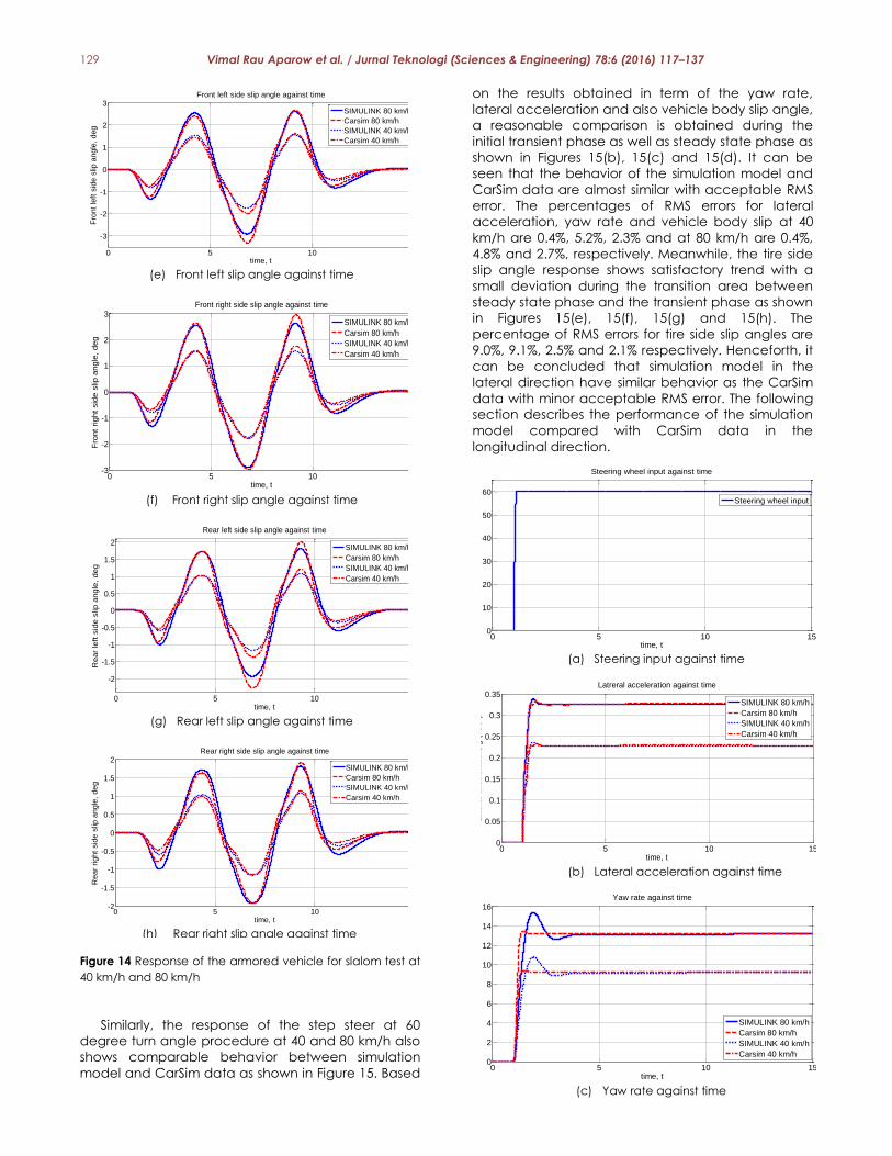
Similarly, the response of the step steer at 60
degree turn angle procedure at 40 and 80 km/h also
shows comparable behavior between simulation
model and CarSim data as shown in Figure 15. Based
on the results obtained in term of the yaw rate,
lateral acceleration and also vehicle body slip angle,
a reasonable comparison is obtained during the
initial transient phase as well as steady state phase as
shown in Figures 15(b), 15(c) and 15(d). It can be
seen that the behavior of the simulation model and
CarSim data are almost similar with acceptable RMS
error. The percentages of RMS errors for lateral
acceleration, yaw rate and vehicle body slip at 40
km/h are 0.4%, 5.2%, 2.3% and at 80 km/h are 0.4%,
4.8% and 2.7%, respectively. Meanwhile, the tire side
slip angle response shows satisfactory trend with a
small deviation during the transition area between
steady state phase and the transient phase as shown
in Figures 15(e), 15(f), 15(g) and 15(h). The
percentage of RMS errors for tire side slip angles are
9.0%, 9.1%, 2.5% and 2.1% respectively. Henceforth, it
can be concluded that simulation model in the
lateral direction have similar behavior as the CarSim
data with minor acceptable RMS error. The following
section describes the performance of the simulation
model compared with CarSim data in the
longitudinal direction.
(e) Front left slip angle against time
(f) Front right slip angle against time
(g) Rear left slip angle against time
(h) Rear right slip angle against time
0 5 10 15
-3
-2
-1
0
1
2
3
time, t
Fro
nt
left
sid
e s
lip a
ngle
, d
eg
Front left side slip angle against time
SIMULINK 80 km/h
Carsim 80 km/h
SIMULINK 40 km/h
Carsim 40 km/h
0 5 10 15-3
-2
-1
0
1
2
3
time, t
Fro
nt
right
sid
e s
lip a
ngle
, deg
Front right side slip angle against time
SIMULINK 80 km/h
Carsim 80 km/h
SIMULINK 40 km/h
Carsim 40 km/h
0 5 10 15
-2
-1.5
-1
-0.5
0
0.5
1
1.5
2
time, t
Re
ar
left
sid
e s
lip
an
gle
, d
eg
Rear left side slip angle against time
SIMULINK 80 km/h
Carsim 80 km/h
SIMULINK 40 km/h
Carsim 40 km/h
0 5 10 15-2
-1.5
-1
-0.5
0
0.5
1
1.5
2
time, t
Rear
right
sid
e s
lip a
ngle
, deg
Rear right side slip angle against time
SIMULINK 80 km/h
Carsim 80 km/h
SIMULINK 40 km/h
Carsim 40 km/h
(a) Steering input against time
(b) Lateral acceleration against time
(c) Yaw rate against time
0 5 10 150
10
20
30
40
50
60
time, t
Ste
erin
g w
he
el a
ngle
, d
eg
Steering wheel input against time
Steering wheel input
0 5 10 150
0.05
0.1
0.15
0.2
0.25
0.3
0.35
time, t
Late
ral accele
ration,
g (
m/s
2)
Latreral acceleration against time
SIMULINK 80 km/h
Carsim 80 km/h
SIMULINK 40 km/h
Carsim 40 km/h
0 5 10 150
2
4
6
8
10
12
14
16
time, t
Yaw
rate
, deg/s
ec
Yaw rate against time
SIMULINK 80 km/h
Carsim 80 km/h
SIMULINK 40 km/h
Carsim 40 km/h
130 Vimal Rau Aparow et al. / Jurnal Teknologi (Sciences & Engineering) 78:6 (2016) 117–137
Figure 15 Response of the armored vehicle for step steer test
at 60 km/h and 80 km/h
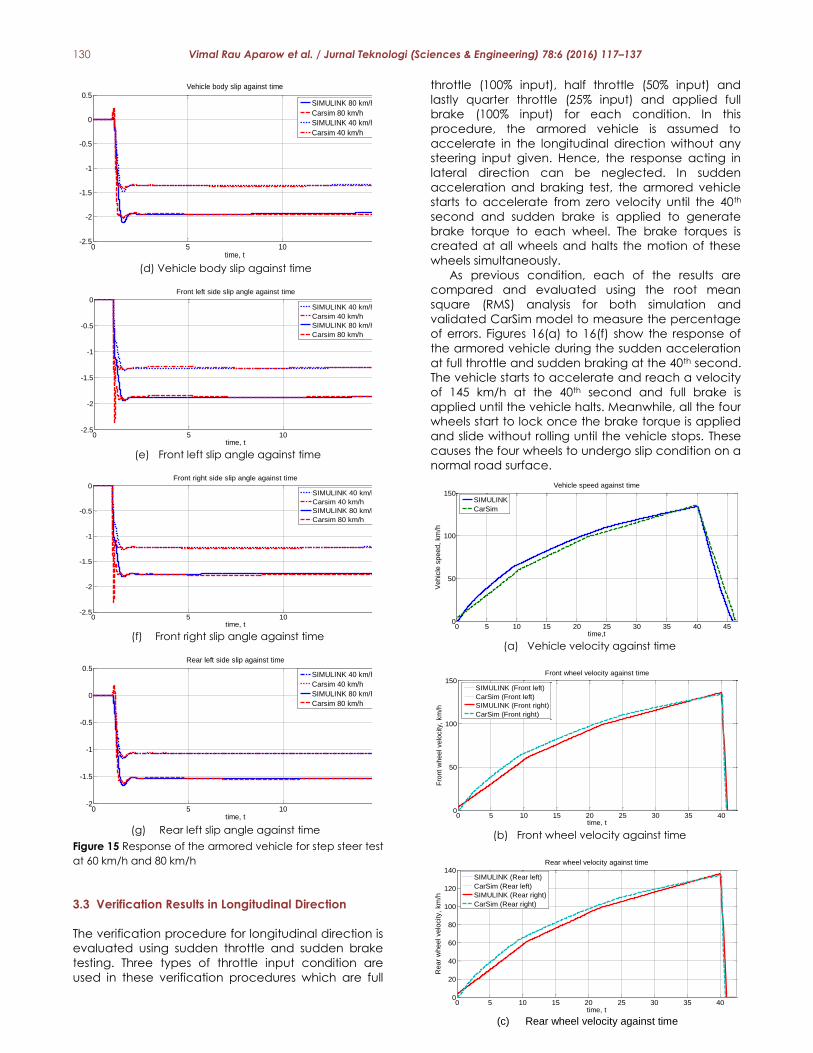
3.3 Verification Results in Longitudinal Direction
The verification procedure for longitudinal direction is
evaluated using sudden throttle and sudden brake
testing. Three types of throttle input condition are
used in these verification procedures which are full
throttle (100% input), half throttle (50% input) and
lastly quarter throttle (25% input) and applied full
brake (100% input) for each condition. In this
procedure, the armored vehicle is assumed to
accelerate in the longitudinal direction without any
steering input given. Hence, the response acting in
lateral direction can be neglected. In sudden
acceleration and braking test, the armored vehicle
starts to accelerate from zero velocity until the 40th
second and sudden brake is applied to generate
brake torque to each wheel. The brake torques is
created at all wheels and halts the motion of these
wheels simultaneously.
As previous condition, each of the results are
compared and evaluated using the root mean
square (RMS) analysis for both simulation and
validated CarSim model to measure the percentage
of errors. Figures 16(a) to 16(f) show the response of
the armored vehicle during the sudden acceleration
at full throttle and sudden braking at the 40th second.
The vehicle starts to accelerate and reach a velocity
of 145 km/h at the 40th second and full brake is
applied until the vehicle halts. Meanwhile, all the four
wheels start to lock once the brake torque is applied
and slide without rolling until the vehicle stops. These
causes the four wheels to undergo slip condition on a
normal road surface.
(d) Vehicle body slip against time
(e) Front left slip angle against time
(f) Front right slip angle against time
(g) Rear left slip angle against time
(h) Rear right slip angle against time
0 5 10 15-2.5
-2
-1.5
-1
-0.5
0
0.5
time, t
Ve
hic
le b
ody s
lip
, d
eg
Vehicle body slip against time
SIMULINK 80 km/h
Carsim 80 km/h
SIMULINK 40 km/h
Carsim 40 km/h
0 5 10 15-2.5
-2
-1.5
-1
-0.5
0
time, t
Fro
nt
left
sid
e s
lip a
ngle
, deg
Front left side slip angle against time
SIMULINK 40 km/h
Carsim 40 km/h
SIMULINK 80 km/h
Carsim 80 km/h
0 5 10 15-2.5
-2
-1.5
-1
-0.5
0
time, t
Fro
nt
rig
ht
sid
e s
lip a
ngle
, d
eg
Front right side slip angle against time
SIMULINK 40 km/h
Carsim 40 km/h
SIMULINK 80 km/h
Carsim 80 km/h
0 5 10 15-2
-1.5
-1
-0.5
0
0.5
time, t
Rear
left
sid
e s
lip a
ngle
, deg
Rear left side slip against time
SIMULINK 40 km/h
Carsim 40 km/h
SIMULINK 80 km/h
Carsim 80 km/h
0 5 10 15-2
-1.5
-1
-0.5
0
0.5
time, t
Re
ar
rig
ht
sid
e s
lip
an
gle
, d
eg
Rear right side slip angle against time
SIMULINK 40 km/h
Carsim 40 km/h
SIMULINK 80 km/h
Carsim 80 km/h
(a) Vehicle velocity against time
(b) Front wheel velocity against time
(c) Rear wheel velocity against time
0 5 10 15 20 25 30 35 40 450
50
100
150
time,t
Ve
hic
le s
pe
ed
, km
/h
Vehicle speed against time
SIMULINK
CarSim
0 5 10 15 20 25 30 35 400
50
100
150
time, t
Fro
nt
wh
eel ve
locity,
km
/h
Front wheel velocity against time
SIMULINK (Front left)
CarSim (Front left)
SIMULINK (Front right)
CarSim (Front right)
0 5 10 15 20 25 30 35 400
20
40
60
80
100
120
140
time, t
Re
ar
wh
eel ve
locity,
km
/h
Rear wheel velocity against time
SIMULINK (Rear left)
CarSim (Rear left)
SIMULINK (Rear right)
CarSim (Rear right)
131 Vimal Rau Aparow et al. / Jurnal Teknologi (Sciences & Engineering) 78:6 (2016) 117–137
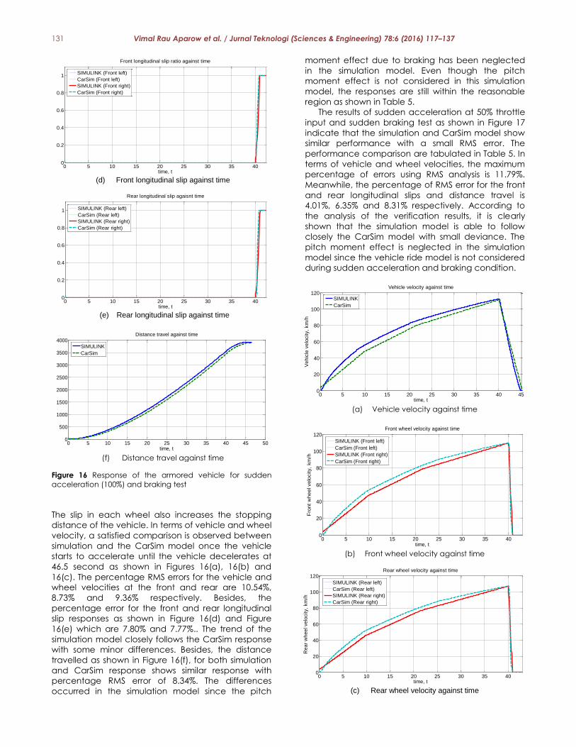
Figure 16 Response of the armored vehicle for sudden
acceleration (100%) and braking test
The slip in each wheel also increases the stopping
distance of the vehicle. In terms of vehicle and wheel
velocity, a satisfied comparison is observed between
simulation and the CarSim model once the vehicle
starts to accelerate until the vehicle decelerates at
46.5 second as shown in Figures 16(a), 16(b) and
16(c). The percentage RMS errors for the vehicle and
wheel velocities at the front and rear are 10.54%,
8.73% and 9.36% respectively. Besides, the
percentage error for the front and rear longitudinal
slip responses as shown in Figure 16(d) and Figure
16(e) which are 7.80% and 7.77%.. The trend of the
simulation model closely follows the CarSim response
with some minor differences. Besides, the distance
travelled as shown in Figure 16(f), for both simulation
and CarSim response shows similar response with
percentage RMS error of 8.34%. The differences
occurred in the simulation model since the pitch
moment effect due to braking has been neglected
in the simulation model. Even though the pitch
moment effect is not considered in this simulation
model, the responses are still within the reasonable
region as shown in Table 5.
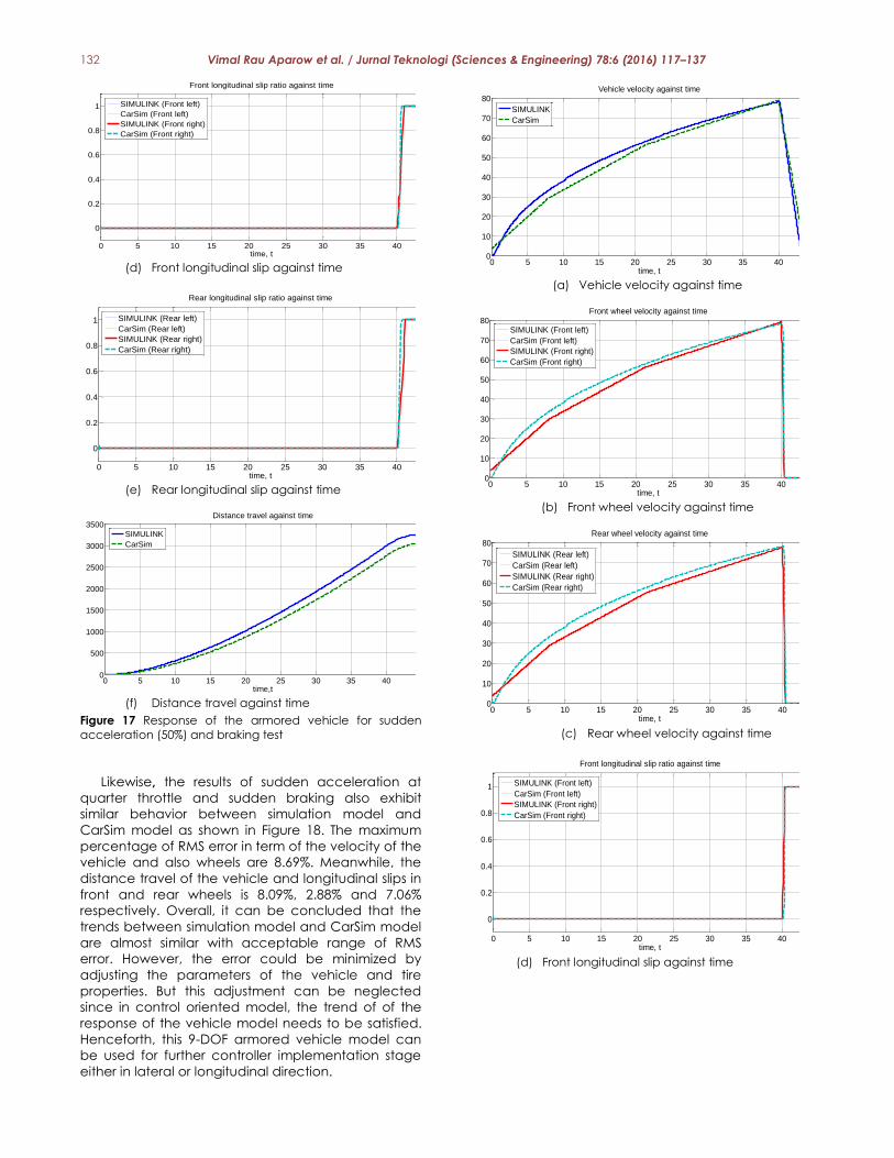
The results of sudden acceleration at 50% throttle
input and sudden braking test as shown in Figure 17
indicate that the simulation and CarSim model show
similar performance with a small RMS error. The
performance comparison are tabulated in Table 5. In
terms of vehicle and wheel velocities, the maximum
percentage of errors using RMS analysis is 11.79%.
Meanwhile, the percentage of RMS error for the front
and rear longitudinal slips and distance travel is
4.01%, 6.35% and 8.31% respectively. According to
the analysis of the verification results, it is clearly
shown that the simulation model is able to follow
closely the CarSim model with small deviance. The
pitch moment effect is neglected in the simulation
model since the vehicle ride model is not considered
during sudden acceleration and braking condition.
(d) Front longitudinal slip against time
(e) Rear longitudinal slip against time
(f) Distance travel against time
0 5 10 15 20 25 30 35 400
0.2
0.4
0.6
0.8
1
time, t
Fro
nt
long
itu
din
al slip
ra
tio
Front longitudinal slip ratio against time
SIMULINK (Front left)
CarSim (Front left)
SIMULINK (Front right)
CarSim (Front right)
0 5 10 15 20 25 30 35 400
0.2
0.4
0.6
0.8
1
time, t
Re
ar
long
itu
din
al slip
ra
tio
Rear longitudinal slip agaisnt time
SIMULINK (Rear left)
CarSim (Rear left)
SIMULINK (Rear right)
CarSim (Rear right)
0 5 10 15 20 25 30 35 40 45 500
500
1000
1500
2000
2500
3000
3500
4000
time, t
dis
tance t
ravel, m
Distance travel against time
SIMULINK
CarSim
(a) Vehicle velocity against time
(b) Front wheel velocity against time
(c) Rear wheel velocity against time
0 5 10 15 20 25 30 35 40 450
20
40
60
80
100
120
time, t
Ve
hic
le v
elo
city,
km
/h
Vehicle velocity against time
SIMULINK
CarSim
0 5 10 15 20 25 30 35 400
20
40
60
80
100
120
time, t
Fro
nt
wh
eel ve
locity,
km
/h
Front wheel velocity against time
SIMULINK (Front left)
CarSim (Front left)
SIMULINK (Front right)
CarSim (Front right)
0 5 10 15 20 25 30 35 400
20
40
60
80
100
120Rear wheel velocity against time
time, t
Re
ar
wh
eel ve
locity,
km
/h
SIMULINK (Rear left)
CarSim (Rear left)
SIMULINK (Rear right)
CarSim (Rear right)
132 Vimal Rau Aparow et al. / Jurnal Teknologi (Sciences & Engineering) 78:6 (2016) 117–137
Figure 17 Response of the armored vehicle for sudden
acceleration (50%) and braking test
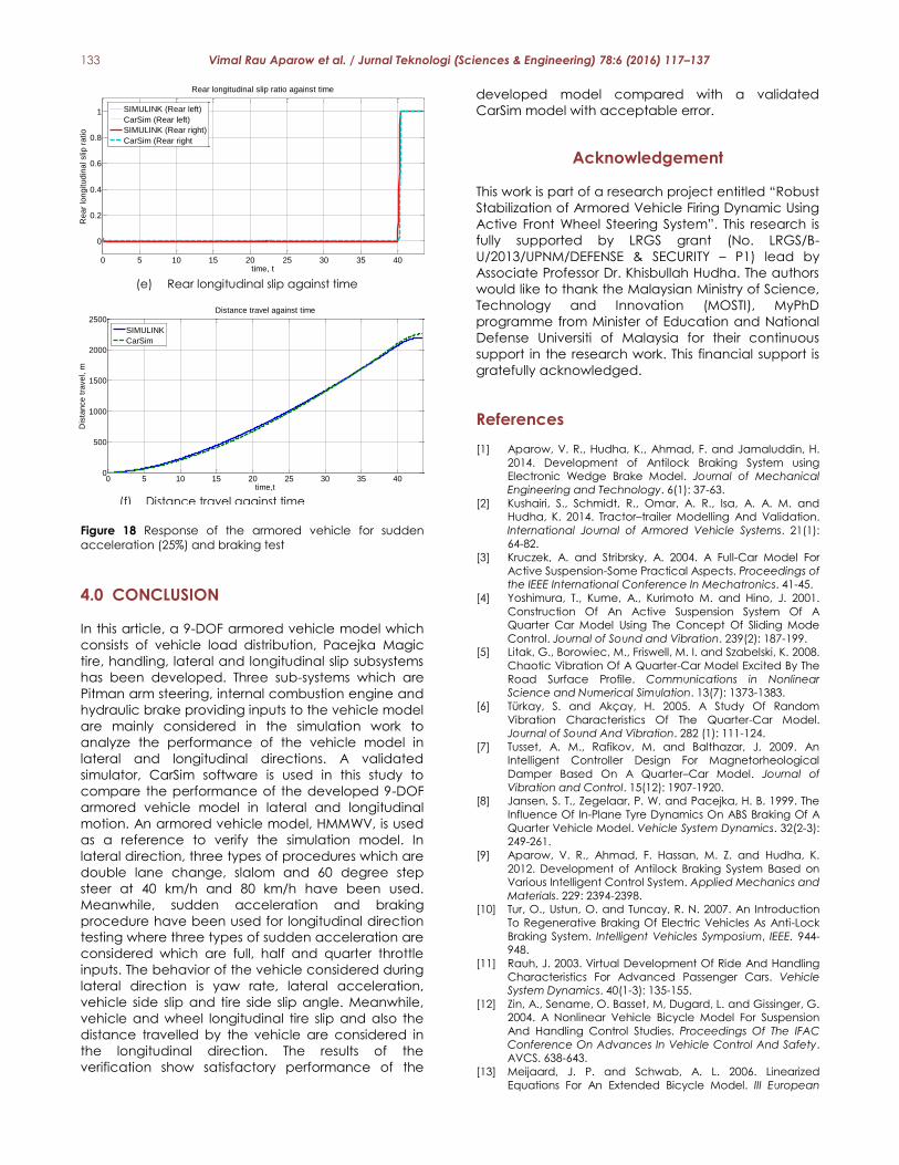
Likewise, the results of sudden acceleration at
quarter throttle and sudden braking also exhibit
similar behavior between simulation model and
CarSim model as shown in Figure 18. The maximum
percentage of RMS error in term of the velocity of the
vehicle and also wheels are 8.69%. Meanwhile, the
distance travel of the vehicle and longitudinal slips in
front and rear wheels is 8.09%, 2.88% and 7.06%
respectively. Overall, it can be concluded that the
trends between simulation model and CarSim model
are almost similar with acceptable range of RMS
error. However, the error could be minimized by
adjusting the parameters of the vehicle and tire
properties. But this adjustment can be neglected
since in control oriented model, the trend of of the
response of the vehicle model needs to be satisfied.
Henceforth, this 9-DOF armored vehicle model can
be used for further controller implementation stage
either in lateral or longitudinal direction.
(d) Front longitudinal slip against time
(e) Rear longitudinal slip against time
(f) Distance travel against time
0 5 10 15 20 25 30 35 40
0
0.2
0.4
0.6
0.8
1
Front longitudinal slip ratio against time
time, t
Fro
nt
long
itu
din
al slip
ra
tio
SIMULINK (Front left)
CarSim (Front left)
SIMULINK (Front right)
CarSim (Front right)
0 5 10 15 20 25 30 35 40
0
0.2
0.4
0.6
0.8
1
time, t
Rear
longitu
din
al slip
ratio
Rear longitudinal slip ratio against time
SIMULINK (Rear left)
CarSim (Rear left)
SIMULINK (Rear right)
CarSim (Rear right)
0 5 10 15 20 25 30 35 40 450
500
1000
1500
2000
2500
3000
3500
time,t
Dis
tance tra
vel, m
Distance travel against time
SIMULINK
CarSim
(a) Vehicle velocity against time
(b) Front wheel velocity against time
(c) Rear wheel velocity against time
(d) Front longitudinal slip against time
0 5 10 15 20 25 30 35 400
10
20
30
40
50
60
70
80
time, t
Vehic
le v
elo
city,
km
/h
Vehicle velocity against time
SIMULINK
CarSim
0 5 10 15 20 25 30 35 400
10
20
30
40
50
60
70
80
time, t
Fro
nt
wheel velo
city,
km
/h
Front wheel velocity against time
SIMULINK (Front left)
CarSim (Front left)
SIMULINK (Front right)
CarSim (Front right)
0 5 10 15 20 25 30 35 400
10
20
30
40
50
60
70
80
time, t
Re
ar
wh
eel ve
locity,
km
/h
Rear wheel velocity against time
SIMULINK (Rear left)
CarSim (Rear left)
SIMULINK (Rear right)
CarSim (Rear right)
0 5 10 15 20 25 30 35 40
0
0.2
0.4
0.6
0.8
1
time, t
Fro
nt
long
itu
din
al slip
ra
tio
Front longitudinal slip ratio against time
SIMULINK (Front left)
CarSim (Front left)
SIMULINK (Front right)
CarSim (Front right)
133 Vimal Rau Aparow et al. / Jurnal Teknologi (Sciences & Engineering) 78:6 (2016) 117–137
Figure 18 Response of the armored vehicle for sudden
acceleration (25%) and braking test
4.0 CONCLUSION
In this article, a 9-DOF armored vehicle model which
consists of vehicle load distribution, Pacejka Magic
tire, handling, lateral and longitudinal slip subsystems
has been developed. Three sub-systems which are
Pitman arm steering, internal combustion engine and
hydraulic brake providing inputs to the vehicle model
are mainly considered in the simulation work to
analyze the performance of the vehicle model in
lateral and longitudinal directions. A validated
simulator, CarSim software is used in this study to
compare the performance of the developed 9-DOF
armored vehicle model in lateral and longitudinal
motion. An armored vehicle model, HMMWV, is used
as a reference to verify the simulation model. In
lateral direction, three types of procedures which are
double lane change, slalom and 60 degree step
steer at 40 km/h and 80 km/h have been used.
Meanwhile, sudden acceleration and braking
procedure have been used for longitudinal direction
testing where three types of sudden acceleration are
considered which are full, half and quarter throttle
inputs. The behavior of the vehicle considered during
lateral direction is yaw rate, lateral acceleration,
vehicle side slip and tire side slip angle. Meanwhile,
vehicle and wheel longitudinal tire slip and also the
distance travelled by the vehicle are considered in
the longitudinal direction. The results of the
verification show satisfactory performance of the
developed model compared with a validated
CarSim model with acceptable error.
Acknowledgement
This work is part of a research project entitled “Robust
Stabilization of Armored Vehicle Firing Dynamic Using
Active Front Wheel Steering System”. This research is
fully supported by LRGS grant (No. LRGS/B-
U/2013/UPNM/DEFENSE & SECURITY – P1) lead by
Associate Professor Dr. Khisbullah Hudha. The authors
would like to thank the Malaysian Ministry of Science,
Technology and Innovation (MOSTI), MyPhD
programme from Minister of Education and National
Defense Universiti of Malaysia for their continuous
support in the research work. This financial support is
gratefully acknowledged.
References
[1] Aparow, V. R., Hudha, K., Ahmad, F. and Jamaluddin, H.
2014. Development of Antilock Braking System using
Electronic Wedge Brake Model. Journal of Mechanical
Engineering and Technology. 6(1): 37-63.
[2] Kushairi, S., Schmidt, R., Omar, A. R., Isa, A. A. M. and
Hudha, K. 2014. Tractor–trailer Modelling And Validation.
International Journal of Armored Vehicle Systems. 21(1):
64-82.
[3] Kruczek, A. and Stribrsky, A. 2004. A Full-Car Model For
Active Suspension-Some Practical Aspects. Proceedings of
the IEEE International Conference In Mechatronics. 41-45.
[4] Yoshimura, T., Kume, A., Kurimoto M. and Hino, J. 2001.
Construction Of An Active Suspension System Of A
Quarter Car Model Using The Concept Of Sliding Mode
Control. Journal of Sound and Vibration. 239(2): 187-199.
[5] Litak, G., Borowiec, M., Friswell, M. I. and Szabelski, K. 2008.
Chaotic Vibration Of A Quarter-Car Model Excited By The
Road Surface Profile. Communications in Nonlinear
Science and Numerical Simulation. 13(7): 1373-1383.
[6] Türkay, S. and Akçay, H. 2005. A Study Of Random
Vibration Characteristics Of The Quarter-Car Model.
Journal of Sound And Vibration. 282 (1): 111-124.
[7] Tusset, A. M., Rafikov, M. and Balthazar, J. 2009. An
Intelligent Controller Design For Magnetorheological
Damper Based On A Quarter–Car Model. Journal of
Vibration and Control. 15(12): 1907-1920.
[8] Jansen, S. T., Zegelaar, P. W. and Pacejka, H. B. 1999. The
Influence Of In-Plane Tyre Dynamics On ABS Braking Of A
Quarter Vehicle Model. Vehicle System Dynamics. 32(2-3):
249-261.
[9] Aparow, V. R., Ahmad, F. Hassan, M. Z. and Hudha, K.
2012. Development of Antilock Braking System Based on
Various Intelligent Control System. Applied Mechanics and
Materials. 229: 2394-2398.
[10] Tur, O., Ustun, O. and Tuncay, R. N. 2007. An Introduction
To Regenerative Braking Of Electric Vehicles As Anti-Lock
Braking System. Intelligent Vehicles Symposium, IEEE. 944-
948.
[11] Rauh, J. 2003. Virtual Development Of Ride And Handling
Characteristics For Advanced Passenger Cars. Vehicle
System Dynamics. 40(1-3): 135-155.
[12] Zin, A., Sename, O. Basset, M, Dugard, L. and Gissinger, G.
2004. A Nonlinear Vehicle Bicycle Model For Suspension
And Handling Control Studies. Proceedings Of The IFAC
Conference On Advances In Vehicle Control And Safety.
AVCS. 638-643.
[13] Meijaard, J. P. and Schwab, A. L. 2006. Linearized
Equations For An Extended Bicycle Model. III European
(e) Rear longitudinal slip against time
(f) Distance travel against time
0 5 10 15 20 25 30 35 40
0
0.2
0.4
0.6
0.8
1
time, t
Rear
longitudin
al slip
ratio
Rear longitudinal slip ratio against time
SIMULINK (Rear left)
CarSim (Rear left)
SIMULINK (Rear right)
CarSim (Rear right
0 5 10 15 20 25 30 35 400
500
1000
1500
2000
2500
time,t
Dis
tan
ce
tra
ve
l, m
Distance travel against time
SIMULINK
CarSim
134 Vimal Rau Aparow et al. / Jurnal Teknologi (Sciences & Engineering) 78:6 (2016) 117–137
Conference on Computational Mechanics. Springer
Netherlands. 772-790.
[14] Baslamisli, S. C., Polat, I. and Kose, I. E. 2007. Gain
Scheduled Active Steering Control Based On A
Parametric Bicycle Model. Intelligent Vehicles Symposium,
IEEE. 1168-1173.
[15] Thompson, A. G. and Pearce, C. E. M. 2001. Direct
Computation Of The Performance Index For An Optimally
Controlled Active Suspension With Preview Applied To A
Half-Car Model. Vehicle System Dynamics. 35(2): 121-137.
[16] Gao, W., Zhang, N. and Du, H. P. 2007. A Half Car Model
For Dynamic Analysis Of Vehicles With Random
Parameters. Australasian Congress on Applied Mechanics.
ACAM, Brisbane, Australia.
[17] Huang, J. L. and Chen, C. 2010. Road-Adaptive Algorithm
Design Of Half-Car Active Suspension System. Expert
Systems with Applications. 37: 305-312.
[18] Ahmad, F., Hudha, K., Imaduddin, F. and Jamaluddin, H.
2010. Modelling, Validation And Adaptive PID Control With
Pitch Moment Rejection Of Active Suspension System For
Reducing Unwanted Vehicle Motion In Longitudinal
Direction. International Journal of Vehicle Systems
Modelling and Testing. 5(4): 312-346.
[19] Hudha, K. Kadir, Z. A. and Jamaluddin, H. 2014. Simulation
And Experimental Evaluations On The Performance Of
Pneumatically Actuated Active Roll Control Suspension
System For Improving Vehicle Lateral Dynamics
Performance. International Journal of Vehicle Design.
64(1): 72-100.
[20] Aparow, V. R., Ahmad, F., Hudha, K. and Jamaluddin, H.
2013. Modelling And PID Control Of Antilock Braking
System With Wheel Slip Reduction To Improve Braking
Performance. International Journal of Vehicle Safety. 6(3):
265-296.
[21] Hudha, K., Jamaluddin, H. and Samin, P. M. 2008.
Disturbance Rejection Control Of A Light Armoured
Vehicle Using Stability Augmentation Based Active
Suspension System. International Journal of Armored
Vehicle Systems. 15(2): 152-169.
[22] Trikande, M. W., Jagirdar, V. V. and Sujithkumar, M. 2014.
Modelling and Comparison of Semi-Active Control Logics
for Suspension System of 8x8 Armoured Multi-Role Military
Vehicle. Applied Mechanics and Materials. 592: 2165-
2178.
[23] Hudha, K., Kadir, Z. A. Said, M. R. and Jamaluddin, H. 2009.
Modelling, Validation And Roll Moment Rejection Control
Of Pneumatically Actuated Active Roll Control For
Improving Vehicle Lateral Dynamics Performance.
International Journal of Engineering Systems Modelling
and Simulation. 1(2): 122-136.
[24] Ikenaga, S., Lewis, F. L., Campos, J. and Davis, L. 2000.
Active Suspension Control Of Ground Vehicle Based On A
Full Vehicle Model. Proceedings of the 2000 American
Control Conference. Illinois, Chicago. 28–30 June. 6: 4019-
4024.
[25] Short, M., Pont, M. J. and Huang, Q. 2004. Safety and
Reliability of Distributed Embedded Systems Simulation of
Vehicle Longitudinal Dynamics, ESL Technical Report,
University of Leicester.
[26] Bakker, E. Pacejka, H. and Lidnar, L. 1987. A New Tire
Model With Application In Vehicle Dynamic Studies. SAE
Technical Paper, 890087. 101-113.
[27] Ping, E. P., Hudha, K. and Jamaluddin, H. 2010. Automatic
Steering Control For Lanekeeping Manoeuvre: Outer-Loop
And Inner-Loop Control Design. International Journal of
Advanced Mechatronic Systems. 2(5): 350-368.
[28] Pacejka, H., Bakker, E. and Nyborg, L. 1987. Tyre Modelling
For Use In Vehicle Dynamics Studies. SAE Technical Paper,
870421.
[29] Shwetha, G. N., Ramesh, H. R. and Shankapal, S. R. 2013.
Modeling, Simulation And Implementation Of A
Proportional-Derivative Controlled Column-Type EPS.
International Journal of Enhanced Research in Science
Technology & Engineering. ISSN: 2319-7463. 2(9): 10-19.
[30] Liu, A. and Chang, S. 1995. Force Feedback In A
Stationary Driving Simulator. Systems, Man and
Cybernetics, IEEE International Conference on Intelligent
Systems for the 21st Century. 2: 1711-1716.
[31] Proca, A. K. 1998. Identification Of Power Steering System
Dynamic Models. Mechatronics. 8(3): 255-270.
[32] Karnopp, D. Argolis, R. and Rosenberg, R. 2000. System
Dynamis: Modeling and Simulations of Mechatronic
Systems. New York, NY: John Wiley Sons.
[33] Moskwa, J. J.and Hedrick, J. K. 1992. Modeling And
Validation Of Automotive Engines For Control Algorithm
Development. ASME Journal of Mechanisms, Transmissions
and Automation in Design. 114(2): 278-285.
[34] Wahlström, J., and Eriksson, L. 2011. Modelling Diesel
Engines With A Variable-Geometry Turbocharger And
Exhaust Gas Recirculation By Optimization Of Model
Parameters For Capturing Non-Linear System
Dynamics. Proceedings of the Institution of Mechanical
Engineers, Part D: Journal of Automobile Engineering.
225(7): 960-986.
[35] Hedrick, J. K., Mcmahnon, D., Swaroop, D., Garg, V.,
Maciuca, D., Blackman, T. and Yip, P. 1995. Longitudinal
Control Development for IVHS Fully Automated and Semi
automated Systems- Phase 1, PATH Research Report,
University of California, Berkeley.
[36] True, H. (Ed.). 2003. The Dynamics of Vehicles on Roads
and on Tracks. CRC Press Publisher. 37.
[37] Udas, A. 2011. Road Variability And Its Effect On Vehicle
Dynamics Simulation. MSc thesis, University of Iowa, Iowa.
[38] Toffin, D. Reymond, G. Kemeny, A. and Droulez, J. 2003.
Influence Of Steering Wheel Torque Feedback In A
Dynamic Driving Simulator. Proceedings of the driving
simulation conference. October, North America,
Dearborn, USA.
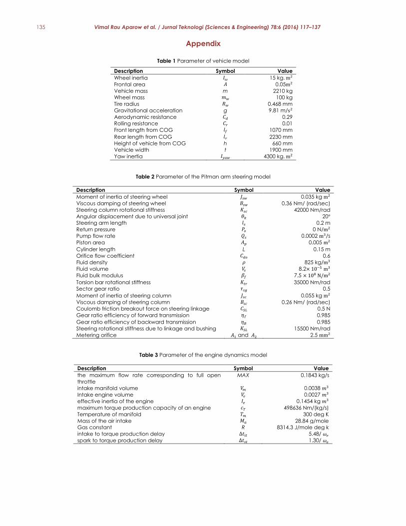
135 Vimal Rau Aparow et al. / Jurnal Teknologi (Sciences & Engineering) 78:6 (2016) 117–137
Appendix
Table 1 Parameter of vehicle model
Description Symbol Value
Wheel inertia 𝐼𝜔 15 kg. m2
Frontal area 𝐴 0.05m2
Vehicle mass m 2210 kg
Wheel mass 𝑚𝑤 100 kg
Tire radius 𝑅𝑤 0.468 mm
Gravitational acceleration g 9.81 m/s2
Aerodynamic resistance 𝐶𝑑 0.29
Rolling resistance 𝐶𝑟 0.01
Front length from COG 𝑙𝑓 1070 mm
Rear length from COG 𝑙𝑟 2230 mm
Height of vehicle from COG h 660 mm
Vehicle width t 1900 mm
Yaw inertia 𝐼𝑦𝑎𝑤 4300 kg. m2
Table 2 Parameter of the Pitman arm steering model
Description Symbol Value
Moment of inertia of steering wheel 𝐽𝑠𝑤 0.035 kg m2
Viscous damping of steering wheel 𝐵𝑠𝑤 0.36 Nm/ (rad/sec)
Steering column rotational stiffness 𝐾𝑠𝑐 42000 Nm/rad
Angular displacement due to universal joint 𝜃𝑘 20° Steering arm length 𝑙𝑠 0.2 m
Return pressure 𝑃𝑜 0 N/m2
Pump flow rate 𝑄𝑠 0.0002 m3/s
Piston area 𝐴𝑝 0.005 m2
Cylinder length L 0.15 m
Orifice flow coefficient 𝐶𝑑𝑜 0.6
Fluid density 𝜌 825 kg/m3
Fluid volume 𝑉𝑠 8.2× 10⁻⁵ m3
Fluid bulk modulus 𝛽𝑓 7.5 × 10⁸ N/m2
Torsion bar rotational stiffness 𝐾𝑡𝑟 35000 Nm/rad
Sector gear ratio 𝜏𝑠𝑔 0.5
Moment of inertia of steering column 𝐽𝑠𝑐 0.055 kg m2
Viscous damping of steering column 𝐵𝑠𝑐 0.26 Nm/ (rad/sec)
Coulomb friction breakout force on steering linkage 𝐶𝑆𝐿 0.5 N
Gear ratio efficiency of forward transmission 𝜂𝑓 0.985
Gear ratio efficiency of backward transmission 𝜂𝐵 0.985
Steering rotational stiffness due to linkage and bushing 𝐾𝑆𝐿 15500 Nm/rad
Metering orifice 𝐴1 and 𝐴2 2.5 mm2
Table 3 Parameter of the engine dynamics model
Description Symbol Value
the maximum flow rate corresponding to full open
throttle
MAX 0.1843 kg/s
intake manifold volume 𝑉𝑚 0.0038 𝑚3
Intake engine volume 𝑉𝑒 0.0027 𝑚3
effective inertia of the engine 𝐼𝑒 0.1454 kg 𝑚3
maximum torque production capacity of an engine 𝑐𝑇 498636 Nm/(kg/s)
Temperature of manifold 𝑇𝑚 300 deg K
Mass of the air intake 𝑀𝑎 28.84 g/mole
Gas constant R 8314.3 J/mole deg k
intake to torque production delay ∆𝑡𝑖𝑡 5.48/ 𝜔𝑒
spark to torque production delay ∆𝑡𝑠𝑡 1.30/ 𝜔𝑒
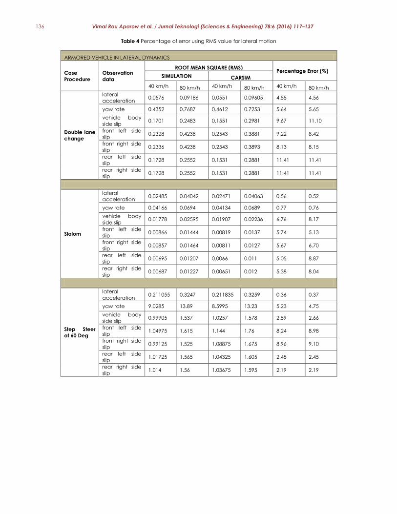
136 Vimal Rau Aparow et al. / Jurnal Teknologi (Sciences & Engineering) 78:6 (2016) 117–137
Table 4 Percentage of error using RMS value for lateral motion
ARMORED VEHICLE IN LATERAL DYNAMICS
Case
Procedure
Observation
data
ROOT MEAN SQUARE (RMS) Percentage Error (%)
SIMULATION CARSIM
40 km/h 80 km/h 40 km/h 80 km/h 40 km/h 80 km/h
Double lane
change
lateral
acceleration 0.0576 0.09186 0.0551 0.09605 4.55 4.56
yaw rate 0.4352 0.7687 0.4612 0.7253 5.64 5.65
vehicle body
side slip 0.1701 0.2483 0.1551 0.2981 9.67 11.10
front left side
slip 0.2328 0.4238 0.2543 0.3881 9.22 8.42
front right side
slip 0.2336 0.4238 0.2543 0.3893 8.13 8.15
rear left side
slip 0.1728 0.2552 0.1531 0.2881 11.41 11.41
rear right side
slip 0.1728 0.2552 0.1531 0.2881 11.41 11.41
Slalom
lateral
acceleration 0.02485 0.04042 0.02471 0.04063 0.56 0.52
yaw rate 0.04166 0.0694 0.04134 0.0689 0.77 0.76
vehicle body
side slip 0.01778 0.02595 0.01907 0.02236 6.76 8.17
front left side
slip 0.00866 0.01444 0.00819 0.0137 5.74 5.13
front right side
slip 0.00857 0.01464 0.00811 0.0127 5.67 6.70
rear left side
slip 0.00695 0.01207 0.0066 0.011 5.05 8.87
rear right side
slip 0.00687 0.01227 0.00651 0.012 5.38 8.04
Step Steer
at 60 Deg
lateral
acceleration 0.211055 0.3247 0.211835 0.3259 0.36 0.37
yaw rate 9.0285 13.89 8.5995 13.23 5.23 4.75
vehicle body
side slip 0.99905 1.537 1.0257 1.578 2.59 2.66
front left side
slip 1.04975 1.615 1.144 1.76 8.24 8.98
front right side
slip 0.99125 1.525 1.08875 1.675 8.96 9.10
rear left side
slip 1.01725 1.565 1.04325 1.605 2.45 2.45
rear right side
slip 1.014 1.56 1.03675 1.595 2.19 2.19
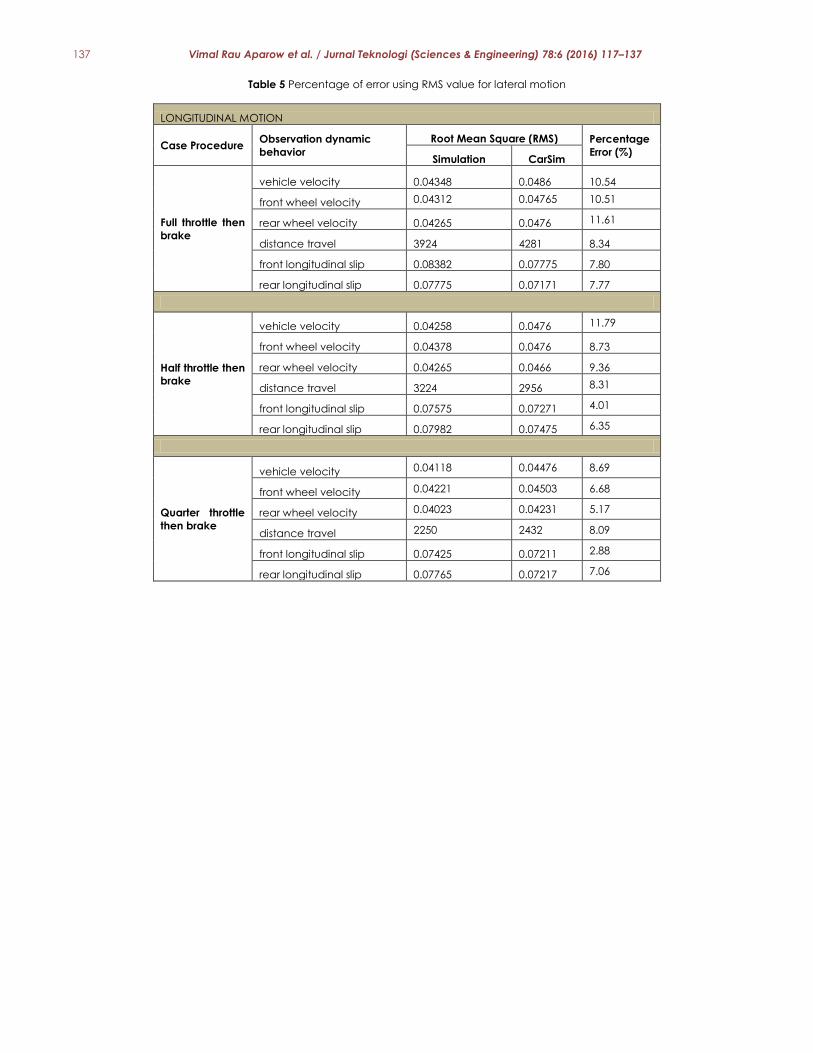
137 Vimal Rau Aparow et al. / Jurnal Teknologi (Sciences & Engineering) 78:6 (2016) 117–137
Table 5 Percentage of error using RMS value for lateral motion
LONGITUDINAL MOTION
Case Procedure Observation dynamic
behavior
Root Mean Square (RMS) Percentage
Error (%) Simulation CarSim
Full throttle then
brake
vehicle velocity 0.04348 0.0486 10.54
front wheel velocity 0.04312 0.04765 10.51
rear wheel velocity 0.04265 0.0476 11.61
distance travel 3924 4281 8.34
front longitudinal slip 0.08382 0.07775 7.80
rear longitudinal slip 0.07775 0.07171 7.77
Half throttle then
brake
vehicle velocity 0.04258 0.0476 11.79
front wheel velocity 0.04378 0.0476 8.73
rear wheel velocity 0.04265 0.0466 9.36
distance travel 3224 2956 8.31
front longitudinal slip 0.07575 0.07271 4.01
rear longitudinal slip 0.07982 0.07475 6.35
Quarter throttle
then brake
vehicle velocity 0.04118 0.04476 8.69
front wheel velocity 0.04221 0.04503 6.68
rear wheel velocity 0.04023 0.04231 5.17
distance travel 2250 2432 8.09
front longitudinal slip 0.07425 0.07211 2.88
rear longitudinal slip 0.07765 0.07217 7.06