Embed Size (px)
Citation preview
Atsushi FujimoriUniversity of Yamanashi
Japan
1. Introduction
Recently, unmanned aerial vehicles (UAVs) have been developed for the purposes of scientificobservations, detecting disasters, surveillance of traffic and army objectives (Wilson, 2007;Langelaan & Rock, 2005; Cho et al., 2005). This paper presents an autonomous flight controldesign to give insights for developing helicopter-type UAVs.A Helicopter is generally an unstable aircraft. Once it is stalled, it is not easy to recoverits attitude. A control system is therefore needed to keep the vehicle stable during flight(Bramwell, 1976; Padfield, 1996; Johnson & Kannan, 2005). This paper presents a flightcontrol design for the longitudinal motion of helicopter to establish autopilot techniques ofhelicopters. The flight mission considered in this paper is that a helicopter hovers at a startposition, moves to a goal position with keeping a specified cruise velocity and hovers again atthe goal. The characteristics of the linearized equation of the helicopter is changed during thisflight mission because the trim values of the equation are widely varied. Gain scheduling (GS)is one of candidates to stabilize the vehicle for the entire flight region. In this paper, a flightcontrol system is designed as follows. The flight control system is constructed as a doubleloop control system (Fujimori et al., 1999; Fujimori et al., 2002) which consists of an inner-loopcontroller and an outer-loop controller. The former is needed for stabilizing the controlledplant, while the latter is used for tracking the reference which is given to accomplish theflight mission. To design the inner-loop controller, the longitudinal motion of a helicopter isfirst modeled by a linear interpolative polytopic model whose varying parameter is the flightvelocity. A GS state feedback law is then designed by linear matrix inequality (LMI) (Boydet al., 1994; Fujimori et al., 2007) so as to stabilize the polytopic model for the entire flightregion. On the other hand, the outer-loop controller is designed by taking into considerationthe steady-state of the controlled variable.The rest of this paper is organized as follows. Section 2 shows equations of the longitudinalmotion of helicopter. Section 3 gives a flight mission and shows a double loop control systemadopted in this paper. The details of the controller designs are presented in Section 4. Section5 shows computer simulation in Matlab/Simulink to evaluate the proposed flight controlsystem. Concluding remarks are given in Section 6.
Autonomous Flight Control System for Longitudinal Motion of a Helicopter
10
www.intechopen.com
tip path plane
horizontal plane
control plane
x
z
V
u w−θ
ε
−θ
V
αd
θc
x
a1
αc
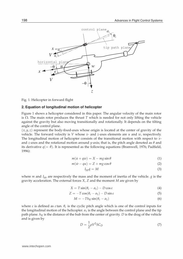
Fig. 1. Helicopter in forward flight
2. Equation of longitudinal motion of helicopter
Figure 1 shows a helicopter considered in this paper. The angular velocity of the main rotoris Ω. The main rotor produces the thrust T which is needed for not only lifting the vehicleagainst the gravity but also moving transitionally and rotationally. It depends on the tiltingangle of the control plane.(x, y, z) represent the body-fixed-axes whose origin is located at the center of gravity of thevehicle. The forward velocity is V whose x- and z-axes elements are u and w, respectively.The longitudinal motion of helicopter consists of the transitional motion with respect to x-and z-axes and the rotational motion around y-axis; that is, the pitch angle denoted as θ andits derivative q(= θ). It is represented as the following equations (Bramwell, 1976; Padfield,1996):
m(u + qw) = X − mg sin θ (1)
m(w − qu) = Z + mg cos θ (2)
Iyy q = M (3)
where m and Iyy are respectively the mass and the moment of inertia of the vehicle. g is thegravity acceleration. The external forces X, Z and the moment M are given by
X = T sin(θc − a1) − D cos ε (4)
Z = −T cos(θc − a1) − D sin ε (5)
M = −ThR sin(θc − a1) (6)
where ε is defined as ε tan. θc is the cyclic pitch angle which is one of the control inputs forthe longitudinal motion of the helicopter. a1 is the angle between the control plane and the tippath plane. hR is the distance of the hub from the center of gravity. D is the drag of the vehicleand is given by
D =1
2ρV2SCD (7)
198 Advances in Flight Control Systems
www.intechopen.com

where ρ is the atmospheric density, S the representative area and CD the drag coefficient. Thethrust T can be calculated by integrating the lift over the whole blade. This results in thefollowing expression for the thrust coefficient:
CT△=
T
ρ(ΩR)2πR2=
Nc
4πRClα{(
2
3+ μ2)θ0 − λc − λi} (8)
where
μ△=
V
ΩRcos αc, λc
△=
V
ΩRsin αc, λi
△=
vi
ΩR(9)
αc△= θc − ε (10)
R is the radius of the rotor blades, c the chord length, N the number of the blades and Clα thelift slope of the blades. vi is the induced velocity through the rotor. θ0 is the collective pitchangle which is another control input. According to Van Hoydonck (2003), the dimensionlessinduced velocity λi through the rotor is approximated by
τλi = CT − CTGl(11)
where CTGlis the thrust coefficient which is given by Glauert’s hypotheses. τ is a time constant
of λi.Summarizing the above equations, define the state and the input vectors as
xp△= [u w q θ λi]
T ∈ ℜ5, up△= [θ0 θc]
T ∈ ℜ2. (12)
The equation of the longitudinal motion of the helicopter is then written as
xp = fp(xp, up). (13)
Equation (13) is referred as the nonlinear plant Pnl hereafter.Letting xe and he be horizontal and the vertical positions of the helicopter from the start, theyare given by
xe = u cos θ + w sin θ (14)
he = u sin θ − w cos θ. (15)
Defining ξp as ξp△= [xe he]T , they are compactly given as
ξp = gp(xp). (16)
In this paper, numerical values of the Eurocopter Deutschland Bo105 (Padfield, 1996) wereused in simulation. They are listed in Table 1. Since this paper considers hovering and forwardflight, the trim condition is given in level flight. Letting xp and up be the state and the inputin trim, respectively, f (xp, up) = 0 holds. Figure 2 shows variations of xp and up with respectto the flight velocity V. It is seen that all trim values are changed in the range of V ∈ [0, 60][m/s].
199Autonomous Flight Control System for Longitudinal Motion of a Helicopter
www.intechopen.com

0 20 40 600
20
40
60u [m/s]
0 20 40 60−10
−8
−6
−4
−2
0w [m/s]
0 20 40 60−10
−8
−6
−4
−2
0
θ [deg]
V [m/s]0 20 40 60
0
0.02
0.04
0.06
λi
V [m/s]
(a) States in trim xp
0 20 40 606
7
8
9
10
θ0 [deg]
V [m/s]0 20 40 60
0
1
2
3
4
5
θc [deg]
V [m/s]
(b) Inputs in trim up
Fig. 2. Trim values with respect to forward velocity V
200 Advances in Flight Control Systems
www.intechopen.com

parameter value unit
Clα 6.113 [1/rad]
c 0.27 [m]
m 2200 [kg]
Ibl 231.7 [kgm2]
Iyy 4973.0 [kgm2]
R 4.91 [m]
Ω 44.4 [rad/s]
N 4 [-]
CDS 1.5 [m2]
hR 1.48 [m]
Table 1. Parameters of Bo105 (Padfield, 1996)
Vc1
0tc1 tc3tc2 tc4 t
Vc2
Vr
tc5
Fig. 3. Flight velocity profile Vr
3. Construction of flight control system
Let the start position be the origin of the coordinates (xe, he). A flight mission considered inthis paper is to navigate the helicopter from the start (0,0) to the goal, denoted as (xr, hr),with keeping its attitude stable. To design a control system, the followings are assumed to besatisfied:
(i) The motion in y-axis direction is not taken into account.
(ii) xp is measurable.
(iii) The trim values xp and up are known in advance.
To realize the flight mission, this paper constructs a tracking control system whose controlledvariable is the flight velocity. The flight region is divided into six phases with respect to theflight velocity as shown in Fig. 3. They are referred as follows.
201Autonomous Flight Control System for Longitudinal Motion of a Helicopter
www.intechopen.com

Pnl[E -F]KoutKpgp
Kin zpupvzr ξp
ξrxp
+
--
+++
Fig. 4. Flight control system
0 ≤ t < tc1 : initial hovering phase
tc1 ≤ t < tc2 : acceleration phase
tc2 ≤ t < tc3 : cruise phase
tc3 ≤ t < tc4 : deceleration phase
tc4 ≤ t < tc5 : low speed phase
tc5 ≤ t : approach phase
From the initial hovering phase to the low speed phase, the reference of the flight velocityis given by Vr shown in Fig. 3. In this paper, the total time of the flight is not cared. But theintegrated value of Vr for t ∈ [0, tc5] must be less than xr not to overtake the goal before theapproach phase. In the approach phase, the reference is generated to meet the position of thehelicopter ξp = [xe he]T with the goal ξr = [xr hr]T .Taking into consideration the above, a double loop control system (Fujimori et al., 1999;Fujimori et al., 2002) is used as a flight control system in this paper. It is shown in Fig. 4. Pnl
represents the nonlinear helicopter dynamics given by Eq. (13), Kin is the inner-loop controller,Kout is the outer-loop controller and Kp is a gain. The controlled variable from the initial
hovering phase to the low speed phase is given by zp△= [u w]T and its reference is given
by zr△= [ur wr]T . In the approach phase, another loop is added outside of (zr − zp)-loop,
where ξp△= [xe he]T is the controlled variable and ξr
△= [xr hr]T is its reference.
Kin consists ofKin = [E − F] (17)
where E is a feedforward gain for tracking the reference, while F is a feedback gainfor stabilizing the plant. Since the trim values are widely varied as shown in Fig. 2, thecharacteristics of the linearized plant is also varied. Then, F is designed by a GS techniquein terms of LMI formulation (Boyd et al., 1994).The reference zr from the initial hovering phase to the low speed phase is generated by theflight velocity profile shown in Fig. 3, and zr in the approach phase is derived from thepositional error ξr − ξp. The switch of the reference is done at t = tc5.
4. Design of control system
4.1 Linear interpolative polytopic model
The objective of flight control in this paper is that the controlled variable is regulated to thespecified trim condition. Linearized models along with the trim is therefore used for controllerdesign. Letting xp(V), up(V) be respectively the state and the input in trim where the flight
202 Advances in Flight Control Systems
www.intechopen.com

velocity is V, the perturbed state and the input are defined as
δxp(t)△= xp(t) − xp(V), δup(t)
△= up(t) − up(V) (18)
The linearized equation of Eq. (13) is then given as
δxp(t) = Ap(V)δxp(t) + Bp(V)δup(t) (19)
where
Ap(V)△=
∂ fp(xp, up)
∂xTp
, Bp(V)△=
∂ fp(xp, up)
∂uTp
. (20)
Although matrices Ap and Bp are functions with respect to V, it is hard to get their explicitrepresentations because of complicated dependence of V as described in Section 2. Then, Ap
and Bp are approximated by interpolating multiple linearized models in the trim condition.For the range of the flight velocity V ∈ [0, Vu], r points {V1, · · · , Vr}, called the operatingpoints, are chosen as
0 ≤ V1 < · · · < Vr ≤ Vu. (21)
The linearized model for V = Vi is a local LTI model representing the plant near the i-thoperating point. Linearly interpolating them, a global model over the entire range of the flightvelocity is constructed as
⎧
⎨
⎩
δxp(t) = Ap(V)δxp(t) + Bp(V)δup(t)
zp(t) = Cpδxp(t) + zp(V)(22)
where
Ap(V) =r
∑i=1
μi(V)Api, Bp(V) =r
∑i=1
μi(V)Bpi,
Cp =
⎡
⎣
1 0 0 0 0
0 1 0 0 0
⎤
⎦ . (23)
μi(V) satisfies the following relations.
0 ≤ μi(V) ≤ 1 (i = 1, · · · , r) (24)
r
∑i=1
μi(V) = 1 (25)
Equation (22) with Eq. (23) is called the linear interpolative polytopic model in this paper.
4.2 Design of Kin
Under assumption (ii), consider a state feedback law
δup(t) = −F(V)δxp(t) + E(V)v(t) (26)
203Autonomous Flight Control System for Longitudinal Motion of a Helicopter
www.intechopen.com
where v is a feedforward input for tracking zr and is given by v = zr − zp when designingKin. The closed-loop system combining Eq. (26) with Eq. (22) is given by
⎧
⎨
⎩
δxp(t) = AF(V)δxp(t) + Bp(V)E(V)v(t)
zp(t) = Cp(V)δxp(t) + Dp(V)E(V)v(t) + zp(V)(27)
AF(V)△= Ap(V) − Bp(V)F(V).
The steady-state controlled variable is given by
zp(∞) = −Cp A−1F BpEv + zp. (28)
v is then given so as to meet zp(∞) with the reference zr; that is, zp(∞) → zr. E is designed as
E = −(Cp A−1F Bp)
−1. (29)
Next, F(V) is designed so that the closed-loop system is stable over the entire flight range andH2 cost is globally suppressed (Fujimori et al., 2007). The controlled plant is newly given by
⎧
⎨
⎩
δxp(t) = Ap(V)δxp(t) + Bp(V)δup(t) + B1(V)w1(t)
z1(t) = C1(V)δxp(t) + D1(V)δup(t)(30)
where z1 and w1 are respectively the input and the output variable for evaluating H2 cost.B1(V), C1(V) and D1(V) are matrices corresponding to z1 and w1. Substituting Eq. (26)without v into Eq. (30), the closed-loop system is
⎧
⎨
⎩
δxp(t) = AF(V)δxp(t) + B1(V)w1(t)
z1(t) = C1F(V)δxp(t)(31)
C1F(V)△= C1(V) − D1(V)F(V).
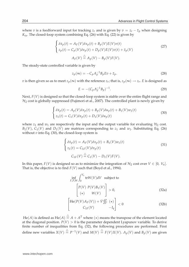
In this paper, F(V) is designed so as to minimize the integration of H2 cost over V ∈ [0, Vu].That is, the objective is to find F(V) such that (Boyd et al., 1994).
infF,P,W
∫ Vu
0trW(V)dV subject to
⎡
⎣
P(V) P(V)B1(V)
(�) W(V)
⎤
⎦ > 0, (32a)
⎡
⎣
He(P(V)AF(V)) + V dPdV (�)
C1F(V) −Iq
⎤
⎦ < 0 (32b)
He(A) is defined as He(A)△= A + AT where (�) means the transpose of the element located
at the diagonal position. P(V) > 0 is the parameter dependent Lyapunov variable. To derivefinite number of inequalities from Eq. (32), the following procedures are performed. First
define new variables X(V)△= P−1(V) and M(V)
△= F(V)X(V). Ap(V) and Bp(V) are given
204 Advances in Flight Control Systems
www.intechopen.com
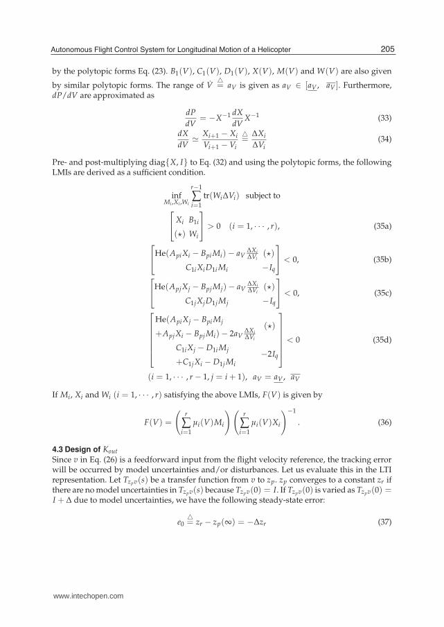
by the polytopic forms Eq. (23). B1(V), C1(V), D1(V), X(V), M(V) and W(V) are also given
by similar polytopic forms. The range of V△= aV is given as aV ∈ [aV , aV ]. Furthermore,
dP/dV are approximated as
dP
dV= −X−1 dX
dVX−1 (33)
dX
dV≃
Xi+1 − Xi
Vi+1 − Vi
△=
∆Xi
∆Vi(34)
Pre- and post-multiplying diag{X, I} to Eq. (32) and using the polytopic forms, the followingLMIs are derived as a sufficient condition.
infMi ,Xi ,Wi
r−1
∑i=1
tr(Wi∆Vi) subject to
⎡
⎣
Xi B1i
(�) Wi
⎤
⎦ > 0 (i = 1, · · · , r), (35a)
⎡
⎣
He(ApiXi − Bpi Mi) − aV∆Xi∆Vi
(�)
C1iXiD1i Mi −Iq
⎤
⎦ < 0, (35b)
⎡
⎣
He(ApjXj − Bpj Mj) − aV∆Xi∆Vi
(�)
C1jXjD1j Mj −Iq
⎤
⎦ < 0, (35c)
⎡
⎢
⎢
⎢
⎢
⎢
⎣
He(ApiXj − Bpi Mj
+ApjXi − Bpj Mi) − 2aV∆Xi∆Vi
(�)
C1iXj − D1i Mj
+C1jXi − D1j Mi
−2Iq
⎤
⎥
⎥
⎥
⎥
⎥
⎦
< 0 (35d)
(i = 1, · · · , r − 1, j = i + 1), aV = aV , aV
If Mi, Xi and Wi (i = 1, · · · , r) satisfying the above LMIs, F(V) is given by
F(V) =
(
r
∑i=1
μi(V)Mi
) (
r
∑i=1
μi(V)Xi
)−1
. (36)
4.3 Design of Kout
Since v in Eq. (26) is a feedforward input from the flight velocity reference, the tracking errorwill be occurred by model uncertainties and/or disturbances. Let us evaluate this in the LTIrepresentation. Let Tzpv(s) be a transfer function from v to zp. zp converges to a constant zr ifthere are no model uncertainties in Tzpv(s) because Tzpv(0) = I. If Tzpv(0) is varied as Tzpv(0) =I + ∆ due to model uncertainties, we have the following steady-state error:
e0△= zr − zp(∞) = −∆zr (37)
205Autonomous Flight Control System for Longitudinal Motion of a Helicopter
www.intechopen.com
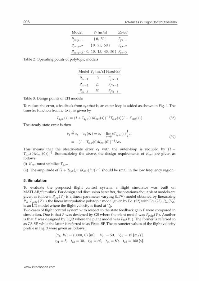
Model Vi [m/s] GS-SF
Ppoly−1 { 0, 50 } Fgs−1
Ppoly−2 { 0, 25, 50 } Fgs−2
Ppoly−3 { 0, 10, 15, 40, 50 } Fgs−3
Table 2. Operating points of polytopic models
Model Vd [m/s] Fixed-SF
Plti−1 0 Ff ix−1
Plti−2 25 Ff ix−2
Plti−3 50 Ff ix−3
Table 3. Design points of LTI models
To reduce the error, a feedback from zp; that is, an outer-loop is added as shown in Fig. 4. Thetransfer function from zr to zp is given by
Tzpzr (s) = (I + Tzpv(s)Kout(s))−1Tzpv(s)(I + Kout(s)) (38)
The steady-state error is then
e1△= zr − zp(∞) = zr − lim
s→0sTzpzr (s)
1
szr
= −(I + Tzpv(0)Kout(0))−1∆zr.
(39)
This means that the steady-state error e1 with the outer-loop is reduced by (I +Tzpv(0)Kout(0))−1. Summarizing the above, the design requirements of Kout are given asfollows:
(i) Kout must stabilize Tzpv.
(ii) The amplitude of (I + Tzpv(jω)Kout(jω))−1 should be small in the low frequency region.
5. Simulation
To evaluate the proposed flight control system, a flight simulator was built onMATLAB/Simulink. For design and discussion hereafter, the notations about plant models aregiven as follows: Plpv(V) is a linear parameter varying (LPV) model obtained by linearizingPnl . Ppoly(V) is the linear interpolative polytopic model given by Eq. (22) with Eq. (23). Plti(Vd)is an LTI model where the flight velocity is fixed at Vd.Two cases of flight control system with respect to the state feedback gain F were compared insimulation. One is that F was designed by GS where the plant model was Ppoly(V). Anotheris that F was designed by LQR where the plant model was Plti(Vd). The former is referred toas GS-SF, while the latter is referred to as Fixed-SF. The parameter values of the flight velocityprofile in Fig. 3 were given as follows:
(xr, hr) = (3000, 0) [m], Vc1 = 50, Vc2 = 15 [m/s],
tc1 = 5, tc2 = 30, tc3 = 60, tc4 = 80, tc5 = 100 [s].
206 Advances in Flight Control Systems
www.intechopen.com
0 10 20 30 40 500
0.2
0.4
0.6
0.8
1
V [m/s]
ν−gap metric between Plti
and Plpv
Plti−1
Plti−2
Plti−3
(a) LTI models
0 10 20 30 40 500
0.1
0.2
0.3
0.4
0.5
V [m/s]
ν−gap metric between Ppoly
and Plpv
Ppoly−1
Ppoly−2
Ppoly−3
(b) polytopic models
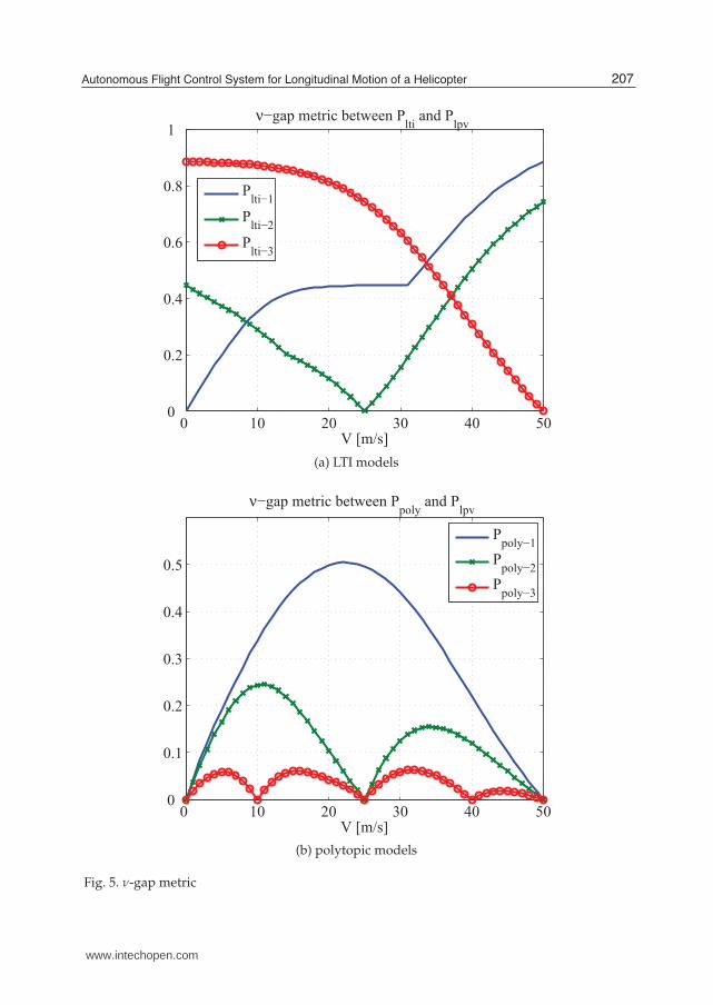
Fig. 5. ν-gap metric
207Autonomous Flight Control System for Longitudinal Motion of a Helicopter
www.intechopen.com
0 10 20 30 40 501.7
1.8
1.9
2
2.1
2.2
2.3
2.4H
2 cost
V [m/s]
Ffix−3
Fgs−1
Fgs−2
Fgs−3
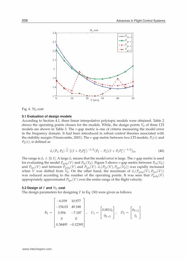
Fig. 6. H2 cost
5.1 Evaluation of design models
According to Section 4.1, three linear interpolative polytopic models were obtained. Table 2shows the operating points chosen for the models. While, the design points Vd of three LTImodels are shown in Table 3. The ν-gap metric is one of criteria measuring the model errorin the frequency domain. It had been introduced in robust control theories associated withthe stability margin (Vinnicombe, 2001). The ν-gap metric between two LTI models, P1(s) andP2(s), is defined as
δν(P1, P2)△= ‖(I + P2P∗
2 )−1/2(P1 − P2)(I + P1P∗1 )−1/2‖∞ (40)
The range is δν ∈ [0, 1]. A large δν means that the model error is large. The ν-gap metric is usedfor evaluating the model Ppoly(V) and Plti(Vd). Figure 5 shows ν-gap metric between Plti(Vd)and Plpv(V) and between Ppoly(V) and Plpv(V). δν(Plti(V), Plpv(Vd)) was rapidly increasedwhen V was shifted from Vd. On the other hand, the maximum of δν(Ppoly(V), Plpv(V))was reduced according to the number of the operating points. It was seen that Ppoly(V)appropriately approximated Plpv(V) over the entire range of the flight velocity.
5.2 Design of F and H2 cost
The design parameters for designing F in Eq. (30) were given as follows.
B1 =
⎡
⎢
⎢
⎢
⎢
⎢
⎢
⎢
⎢
⎣
−6.039 10.977
−154.03 49.188
3.954 −7.187
0 0
0.38495 −0.12395
⎤
⎥
⎥
⎥
⎥
⎥
⎥
⎥
⎥
⎦
, C1 =
⎡
⎣
0.001I5
02×5
⎤
⎦ , D1 =
⎡
⎣
05×2
I2
⎤
⎦
208 Advances in Flight Control Systems
www.intechopen.com

0 50 100 150−20
0
20
40
60
u [m
/s]
Fixed−SF 1
0 50 100 150−30
−20
−10
0
10
w [m
/s]
0 50 100 1505
10
15
20
25
t [s]
θ0 [d
eg]
0 50 100 150−2
0
2
4
6
t [s]
θc
[deg
]
u
ur
w
wr
(a) Controlled variables and inputs
0 20 40 60 80 100 120 1400
1000
2000
3000
Fixed−SF 1
t [s]
xe
[m]
0 20 40 60 80 100 120 140−300
−200
−100
0
100
t [s]
he
[m]
(b) Positions
Fig. 7. Time responses using Ff ix−1
209Autonomous Flight Control System for Longitudinal Motion of a Helicopter
www.intechopen.com

0 50 100 150−20
0
20
40
60
u [m
/s]
Fixed−SF 2
0 50 100 150−30
−20
−10
0
10
w [m
/s]
0 50 100 1505
10
15
20
25
t [s]
θ0 [d
eg]
0 50 100 150−2
0
2
4
6
t [s]
θc
[deg
]
u
ur
w
wr
(a) Controlled variables and inputs
0 20 40 60 80 100 120 1400
1000
2000
3000
Fixed−SF 2
t [s]
xe
[m]
0 20 40 60 80 100 120 140−300
−200
−100
0
100
t [s]
he
[m]
(b) Positions
Fig. 8. Time responses using Ff ix−2
210 Advances in Flight Control Systems
www.intechopen.com
0 50 100 150−20
0
20
40
60
u [m
/s]
Fixed−SF 3
0 50 100 150−30
−20
−10
0
10
w [m
/s]
0 50 100 1505
10
15
20
25
t [s]
θ0 [d
eg]
0 50 100 150−2
0
2
4
6
t [s]
θc
[deg
]
u
ur
w
wr
(a) Controlled variables and inputs
0 20 40 60 80 100 120 1400
1000
2000
3000
Fixed−SF 3
t [s]
xe [
m]
0 20 40 60 80 100 120 140−300
−200
−100
0
100
t [s]
he
[m]
(b) Positions
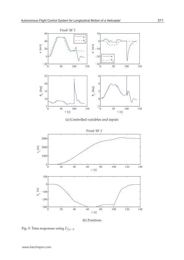
Fig. 9. Time responses using Ff ix−3
211Autonomous Flight Control System for Longitudinal Motion of a Helicopter
www.intechopen.com

0 50 100 150−20
0
20
40
60
u [m
/s]
GS−SF 1
0 50 100 150−30
−20
−10
0
10
w [m
/s]
0 50 100 1505
10
15
20
25
t [s]
θ0 [d
eg]
0 50 100 150−2
0
2
4
6
t [s]
θc
[deg
]
u
ur
w
wr
(a) Controlled variables and inputs
0 20 40 60 80 100 120 1400
1000
2000
3000
GS−SF 1
t [s]
xe
[m]
0 20 40 60 80 100 120 140−300
−200
−100
0
100
t [s]
he
[m]
(b) Positions
Fig. 10. Time responses using Fgs−1
212 Advances in Flight Control Systems
www.intechopen.com

0 50 100 150−20
0
20
40
60
u [m
/s]
GS−SF 2
0 50 100 150−30
−20
−10
0
10
w [m
/s]
0 50 100 1505
10
15
20
25
t [s]
θ0 [d
eg]
0 50 100 150−2
0
2
4
6
t [s]
θc
[deg
]
u
ur
w
wr
(a) Controlled variables and inputs
0 20 40 60 80 100 120 1400
1000
2000
3000
GS−SF 2
t [s]
xe
[m]
0 20 40 60 80 100 120 140−300
−200
−100
0
100
t [s]
he
[m]
(b) Positions
Fig. 11. Time responses using Fgs−2
213Autonomous Flight Control System for Longitudinal Motion of a Helicopter
www.intechopen.com

0 50 100 150−20
0
20
40
60
u [m
/s]
GS−SF 3
0 50 100 150−30
−20
−10
0
10
w [m
/s]
0 50 100 1505
10
15
20
25
t [s]
θ0 [d
eg]
0 50 100 150−2
0
2
4
6
t [s]
θc
[deg
]
u
ur
w
wr
(a) Controlled variables and inputs
0 20 40 60 80 100 120 1400
1000
2000
3000
GS−SF 3
t [s]
xe
[m]
0 20 40 60 80 100 120 140−300
−200
−100
0
100
t [s]
he
[m]
(b) Positions
Fig. 12. Time responses using Fgs−3
214 Advances in Flight Control Systems
www.intechopen.com
They were used for both of GS-SF and Fixed-SF. Three GS-SF gains denoted as Fgs−i (i =1, 2, 3) were designed according to Section 4.2, while three Fixed-SF gains denoted as Ff ix−i
(i = 1, 2, 3) were designed by LQR technique in which the weights of the quadratic indexwere given by CT
1 C1 and DT1 D1.
Figure 6 shows the H2 cost of the closed-loop system which the designed F is combined withEq. (30). The H2 cost by Ff ix−3 was minimized at V = 40 [m/s] which was near the designpoint Vd = 50 [m/s], but was increased in the low flight velocity region. The H2 cost by Ff ix−1
and Ff ix−2 showed the similar result. On the other hand, the H2 cost by Fgs−2 and Fgs−3 waskept small over the entire flight region. The H2 cost by Fgs−1 was small in the middle flightvelocity region but was increased in the low and the high flight velocity regions.
5.3 Tracking evaluation
The flight mission given in Fig. 3 was performed in Simulink. Figures 7 - 12 show the timehistories of the closed-loop system with the three GS-SF and three Fixed-SF gains. In the caseof Ff ix−1 shown in Fig. 7, the controlled variables u and w tracked their references until theacceleration phase (5 ≤ t < 30 [s]) but they were diverged in the cruise phase (30 ≤ t < 60[s]). In the deceleration phase (60 ≤ t < 80 [s]), the closed-loop system was stabilized againbut it was de-stabilized in the approach phase (t ≥ 100 [s]). Although the closed-loop systemremained stable for the entire flight region in the case of Ff ix−2 shown in Fig. 8, oscillatoryresponses were observed in the cruise and approach phases. The responses using Ff ix−3
shown in Fig. 9 were better than those using Ff ix−2.On the other hand, the three GS-SF gains provided stable responses as shown in Figs. 10 -12, In particular, The responses by Fgs−3 showed improved tracking and settling propertiescompared to other cases.Summarizing the simulation in MATLAB/Simulink, polytopic model Ppoly−3 made the ν-gapmetric smaller than other models for the entire flight region. Fgs−3 designed by using Ppoly−3
showed better control performance.
6. Concluding remarks
This paper has presented an autonomous flight control design for the longitudinal motion ofhelicopter to give insights for developing autopilot techniques of helicopter-type UAVs. Thecharacteristics of the equation of helicopter was changed during a specified flight missionbecause the trim values of the equation were widely varied. In this paper, gain schedulingstate feedback (GS-SF) was included in the double loop flight control system to keep thevehicle stable for the entire flight region. The effectiveness of the proposed flight controlsystem was evaluated by computer simulation in MATLAB/Simulink. The model error ofthe polytopic model was smaller than that of LTI models which were obtained at specifiedflight velocity. Flight control systems with GS-SF showed better control performances thanthose with fixed-gain state feedback. The double loop flight control structure was useful foraccomplishing flight mission considered in this paper.
7. References
[1] Boyd, S.; Ghaoui, L. E.; Feron, E. & Balakrishnan, V. (1994). Linear Matrix Inequalities inSystem and Control Theory, SIAM, Vol. 15, Philadelphia.
[2] Bramwell, A. R. S. (1976). Helicopter Dynamics, Edward Arnold, London, 1976.
215Autonomous Flight Control System for Longitudinal Motion of a Helicopter
www.intechopen.com
[3] Cho, S.-J.; Jang, D.-S. & Tahk, M.-L. (2005). Application of TCAS-II for Unmanned AerialVehicles, Proc. CD-ROM of JSASS 19th International Sessions in 43rd Aircraft Symposium,Nagoya, 2005
[4] Fujimori, A.; Kurozumi, M.; Nikiforuk, P. N. & Gupta, M. M. (1999). A Flight ControlDesign of ALFLEX Using Double Loop Control System, AIAA Paper, 99-4057-CP,Guidance, Navigation and Control Conference, 1999, pp. 583-592.
[5] Fujimori, A.; Nikiforuk, P. N. & Gupta, M. M. (2001). A Flight Control Design ofa Reentry Vehicle Using Double Loop Control System with Fuzzy Gain-Scheduling,IMechE Journal of Aerospace Engineering, Vol. 215, No. G1, 2001, pp. 1-12.
[6] Fujimori, A.; Miura, K. & Matsushita, H. (2007). Active Flutter Suppression of aHigh-Aspect-Ratio Aeroelastic Using Gain Scheduling, Transactions of The Japan Societyfor Aeronautical and Space Sciences, Vol. 55, No. 636, 2007, pp. 34-42.
[7] Johnson, E. N. & Kannan, S. K. (2005). Adaptive Trajectory Control for AutonomousHelicopters, Journal of Guidance, Control and Dynamics, Vol. 28, No. 3, 2005, pp. 524-538.
[8] Langelaan, J. & Rock, S. (2005). Navigation of Small UAVs Operating in Forests, Proc.CD-ROM of AIAA Guidance, Navigation, and Control Conference, San Francisco, 2005.
[9] Padfield, G. D. (1996). Helicopter Dynamics: The Theory and Application of Flying Qualitiesand Simulation Modeling, AIAA, Reston, 1996.
[10] Van Hoydonck, W. R. M. (2003). Report of the Helicopter Performance, Stability and ControlPractical AE4-213, Faculty of Aerospace Engineering, Delft University of Technology,2003.
[11] Vinnicombe, G. (2001). Uncertainty and Feedback (H∞ loop-shaping and the ν-gap metric),Imperial College Press, Berlin.
[12] Wilson, J. R. (2007). UAV Worldwide Roundup 2007, Aerospace America, May, 2007, pp.30-38.
216 Advances in Flight Control Systems
www.intechopen.com

Advances in Flight Control SystemsEdited by Dr. Agneta Balint
ISBN 978-953-307-218-0Hard cover, 296 pagesPublisher InTechPublished online 11, April, 2011Published in print edition April, 2011
InTech EuropeUniversity Campus STeP Ri Slavka Krautzeka 83/A 51000 Rijeka, Croatia Phone: +385 (51) 770 447 Fax: +385 (51) 686 166www.intechopen.com
InTech ChinaUnit 405, Office Block, Hotel Equatorial Shanghai No.65, Yan An Road (West), Shanghai, 200040, China
Phone: +86-21-62489820 Fax: +86-21-62489821
Nonlinear problems in flight control have stimulated cooperation among engineers and scientists from a rangeof disciplines. Developments in computer technology allowed for numerical solutions of nonlinear controlproblems, while industrial recognition and applications of nonlinear mathematical models in solvingtechnological problems is increasing. The aim of the book Advances in Flight Control Systems is to bringtogether reputable researchers from different countries in order to provide a comprehensive coverage ofadvanced and modern topics in flight control not yet reflected by other books. This product comprises 14contributions submitted by 38 authors from 11 different countries and areas. It covers most of the currentsmain streams of flight control researches, ranging from adaptive flight control mechanism, fault tolerant flightcontrol, acceleration based flight control, helicopter flight control, comparison of flight control systems andfundamentals. According to these themes the contributions are grouped in six categories, corresponding to sixparts of the book.
How to referenceIn order to correctly reference this scholarly work, feel free to copy and paste the following:
Atsushi Fujimori (2011). Autonomous Flight Control System for Longitudinal Motion of a Helicopter, Advancesin Flight Control Systems, Dr. Agneta Balint (Ed.), ISBN: 978-953-307-218-0, InTech, Available from:http://www.intechopen.com/books/advances-in-flight-control-systems/autonomous-flight-control-system-for-longitudinal-motion-of-a-helicopter

© 2011 The Author(s). Licensee IntechOpen. This chapter is distributedunder the terms of the Creative Commons Attribution-NonCommercial-ShareAlike-3.0 License, which permits use, distribution and reproduction fornon-commercial purposes, provided the original is properly cited andderivative works building on this content are distributed under the samelicense.