3Now at Jacobs Engineering Group, 2155 Louisiana NE, Suite 10000, Albuquerque, NM 87110, (505) 888-1300

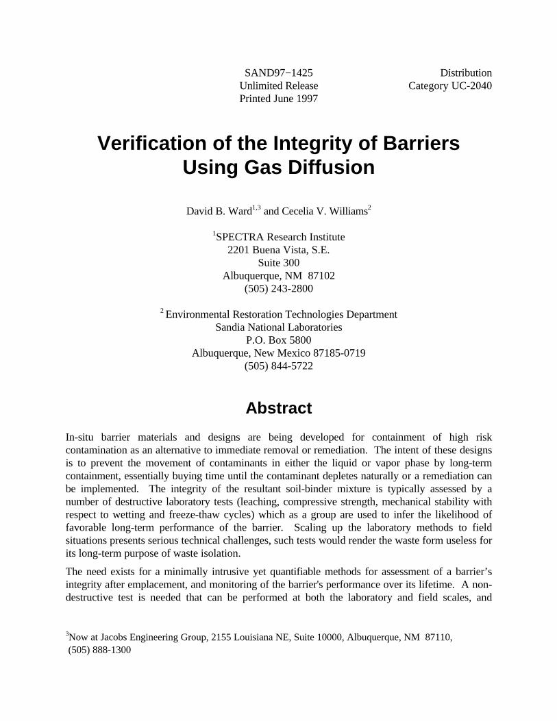
SAND97−1425 DistributionUnlimited Release Category UC-2040Printed June 1997

Verification of the Integrity of BarriersUsing Gas Diffusion

David B. Ward1,3 and Cecelia V. Williams2

1SPECTRA Research Institute2201 Buena Vista, S.E.

Suite 300Albuquerque, NM 87102

(505) 243-2800

2 Environmental Restoration Technologies DepartmentSandia National Laboratories

P.O. Box 5800Albuquerque, New Mexico 87185-0719

(505) 844-5722

Abstract

In-situ barrier materials and designs are being developed for containment of high riskcontamination as an alternative to immediate removal or remediation. The intent of these designsis to prevent the movement of contaminants in either the liquid or vapor phase by long-termcontainment, essentially buying time until the contaminant depletes naturally or a remediation canbe implemented. The integrity of the resultant soil-binder mixture is typically assessed by anumber of destructive laboratory tests (leaching, compressive strength, mechanical stability withrespect to wetting and freeze-thaw cycles) which as a group are used to infer the likelihood offavorable long-term performance of the barrier. Scaling up the laboratory methods to fieldsituations presents serious technical challenges, such tests would render the waste form useless forits long-term purpose of waste isolation.

The need exists for a minimally intrusive yet quantifiable methods for assessment of a barrier’sintegrity after emplacement, and monitoring of the barrier's performance over its lifetime. A non-destructive test is needed that can be performed at both the laboratory and field scales, and

4

that directly measures the properties of interest or is correlated with them. Here, we evaluatenon-destructive measurements of inert-gas diffusion (specifically, SF6) as an indicator of waste-form integrity. Low diffusivity is a desirable waste-form property because migration by diffusionis an important mechanism for contaminant loss, although the net loss rate is also influenced bydissolution and reprecipitation. Diffusion measurements using an inert gas provide conservativeestimates of diffusivity under aqueous conditions. The goals of this project are to show thatdiffusivity can be measured in core samples of soil jet-grouted with Portland cement, validate theexperimental method through measurements on samples, and to calculate aqueous diffusivitiesfrom a series of diffusion measurements.

This study shows that it is practical to measure SF6 diffusion rates in the laboratory on samples ofgrout (Portland cement and soil) typical of what might be used in a barrier. This study hasdemonstrated the at the laboratory scale: (1) SF6 is a nearly ideal tracer — inert with respect tomost materials and readily detectable at trace levels (down to 5 ppb); (2) Diffusion of SF6 into airmay be as rapid as 0.073 cm2/s, based on direct measurement; (2) Diffusion of SF6 through thegrout (Portland cement and soil) is on the order of 0.001–0.003 cm2/s; and (4) Measurements ofeffective diffusion coefficient are reproducible to ± 10% or better. These results suggest thatfield-scale tests would also be feasible, and would provide a non-destructive method of evaluatingthe integrity of a barrier in situ. Diffusion of SF6 through grout (Portland cement and soil) is atleast an order of magnitude slower than through air. The use of this tracer should be sensitive tothe presence of fractures, voids, or other discontinuities in the grout/soil structure. Field-scalemeasurements should be practical on time-scales of a few days.

5

Acknowledgments

Sandia is a multiprogram laboratory operated by Sandia Corporation, a Lockheed MartinCompany, for the United States Department of Energy under Contract DE-AC04-94AL85000.

This effort is funded by the United States Department of Energy, Office of Science andTechnology, through the Subsurface Contaminants Focus Area.

The authors wish to especially thank the following:

Brian Dwyer for allowing us to take core samples from the jet-grouted columns he had emplacedat the cold test areas in TAIII.

Bruce Reavis for helping us core the jet-grouted columns.

Hank Westrich for providing us with the laboratory space.

John Kelly for the surface area analyses.

6

Intentionally Left Blank

7

Contents

Introduction ................................................................................................................................9Experimental Apparatus ............................................................................................................ 11Calculation of Diffusivity from Measurements ........................................................................... 15

Estimation of Hydraulic Conductivity from Diffusion Coefficients........................................ 16Experimental Methods............................................................................................................... 19

Sample Preparation and Descriptions................................................................................... 19Surface Area Determinations ............................................................................................... 28Diffusion Measurement Protocol ......................................................................................... 28

Instrument Operation..................................................................................................... 28Measurement of Samples Requiring Dilution.................................................................. 29Sample Diffusion Measurement...................................................................................... 29

Results ...................................................................................................................................... 30Surface Area Measurements ................................................................................................ 30Calibration Curve ................................................................................................................ 30Measurement of the SF6 Diffusion Coefficient into Air ......................................................... 32Measurements on Core Samples .......................................................................................... 34

Discussion................................................................................................................................. 40Bulk Diffusion Coefficient for SF6 Self-Diffusion ................................................................. 40Measured Bulk Diffusion for SF6 Diffusion into Air ............................................................. 41Expected Time-Dependent Diffusion in Portland Cement..................................................... 41Experimental Measurements and Derived Parameters .......................................................... 43Feasibility of Field-Scale Measurements............................................................................... 45

Summary................................................................................................................................... 47References ................................................................................................................................ 49

Tables

Table 1. Sample descriptions ................................................................................................. 21Table 2. Surface areas by N2-BET ......................................................................................... 30Table 3. Theoretical diffusion rates for SF6............................................................................. 41Table 4. Constants used in calculations .................................................................................. 44Table 5. Measurements and derived parameters ..................................................................... 44

Figures

Figure 1. Diffusion cell............................................................................................................ 12Figure 2. Alternate geometry for the diffusion cell................................................................... 14Figure 3. P36-1a top and bottom surfaces ............................................................................... 24Figure 4. P36-1b top and bottom surfaces ............................................................................... 25Figure 5. P36-2a top and bottom surfaces ............................................................................... 26Figure 6. P36-2b top and bottom surfaces ............................................................................... 27

8

Figure 7. Calibration curve for gas analyzer ............................................................................ 32Figure 8. SF6 bulk diffusion into air (orifice A) ........................................................................ 33Figure 9. SF6 bulk diffusion into air (orifice B) ........................................................................ 34Figure 10. SF6 diffusion profile for P36-1a ................................................................................ 36Figure 11. SF6 diffusion profile for P36-1b ................................................................................ 37Figure 12. SF6 diffusion profile for P36-2a ................................................................................ 38Figure 13. SF6 diffusion profile for P36-2b ................................................................................ 39Figure 14. Expected SF6 diffusion profile using likely estimates of controlling parameters.......... 42

Symbols

A cross-sectional area of the sample — L2

Asp specific surface area of a porous material — L2/MC concentration of SF6 at a specific point — M/L3

C0 initial concentration of SF6 in the supply reservoir — M/L3

CC concentration of SF6 in the collection reservoir — M/L3

d diameter of pressure-equalizing tube — LD0 bulk diffusion coefficient for SF6 (e.g., in air or N2) — L2/TDS effective diffusion coefficient for SF6 in the sample — L2/Tg acceleration due to gravity — L/T2

h piezometric head — LJ SF6 flux (parallel to diffusion-cell or capillary axis) — M/L2/Tk permeability — L2

K hydraulic conductivity — L/TL lengthL length (thickness) of the sample (parallel to flow direction) — Llpe length of pressure-equalizing capillary — LM massm mass of SF6 — MQ total flow rate — L3/TSF6

M Measured SF6 concentration (M/M)SF6

* Corrected SF6 concentration (M/M)SF 6

N Normalized SF6 concentration (M/M)T timet time — Ttlin time after which the linear approximation is valid — TVC volume of collection reservoir — L3

x coordinate along diffusion-cell axis — Lφ porosity — L3/L3

µ dynamic viscosity — M/LTθ tortuosity — L/Lρ density — M/L3

ρm density of the non-porous solid; the matrix density — M/L3

9

Introduction

In-situ barrier emplacement techniques and materials for the containment of high-riskcontaminants in soils are currently being evaluated as an alternative to immediate removal orremediation. Because of their relatively high cost, the barriers are intended to be used in caseswhere the risk is too great to remove the contaminants, the contaminants are too difficult toremove with current technologies, or the potential for movement of the contaminants to the watertable is so high that immediate action needs to be taken to reduce health risks. Consequently,barriers are primarily intended for use in high-risk sites where few viable alternatives exist to stopthe movement of contaminants in the near term.

Under many circumstances, the most expedient and effective means of isolating contaminated soilfrom the environment is through in situ solidification to produce a single cohesive body. Such awaste form, called a barrier, should be mechanically strong and durable, and resistant to leachingof the incorporated waste constituents. Among the numerous solidification agents proposed forvarious sites, the most common ones are Portland cement, sulfur cement, bitumen, andpolyethylene. More exotic binders include colloidal silica, Na-siloxane polymer and acrylicpolymer (3M Co. cement restorer). The integrity of the resultant soil-binder mixture is typicallyassessed by a number of destructive laboratory tests (leaching, compressive strength, mechanicalstability with respect to wetting and freeze-thaw cycles (cf. Franz et al., 1994)), which as a groupare used to infer the likelihood of favorable long-term performance of the barrier.

Assessing the integrity of the barrier once it is emplaced, and during its anticipated life, is adifficult but necessary requirement. Scaling laboratory methods to field situations presents serioustechnical challenges. Compressive strength, which serves as an indicator of mechanical durabilityin all of the laboratory tests, is most readily measured on small samples of uniform dimensions,but the measurements cannot be repeated because each sample is destroyed in the process. Toapply compressive-strength testing at the field scale, the barrier would have to be exhumed andcored at a multitude of points to obtain a statistically valid sampling. Alternatively, the completebarrier could be subjected to some form of impact testing. In either case, such tests would renderthe waste form useless for its long-term purpose of waste isolation. Existing surface-based andborehole geophysical techniques, while providing a “picture” of the barrier, do not provide thedegree of resolution required to assure the formation of an integral in-situ barrier.

A non-destructive test is needed that can be performed at both the laboratory and field scales, andthat directly measures the properties of interest or is correlated with them. Here, we evaluatenon-destructive measurements of inert-gas diffusion (specifically, SF6) as an indicator of waste-form integrity. In the use of tracers for barrier verification it is important to understand how atracer gas injected into the barrier volume will diffuse. For a tracer system to work, the tracermust 1) diffuse at significantly different rates through the barrier material compared with thesurrounding medium so that breaches in the barrier will be readily detectable; 2) diffuse at a highenough rate such that monitors outside the barrier can be spaced at relatively large intervals fromone another and still be able to detect the tracer in reasonable periods of time; and 3) diffuse at a

10

predictable rate given the soil characteristics. To determine if these diffusion assumptions arevalid, a series of bench scale tests was performed.

Low diffusivity is a desirable waste-form property because migration by diffusion is an importantmechanism for contaminant loss, although the net loss rate is also influenced by dissolution andreprecipitation. At the microscopic scale, diffusivity is a function of the connected porosity and ageometric factor, the tortuosity. At larger scales, additional factors must be considered, includingthe presence of voids and fractures, as well as heterogeneities due to incomplete mixing of thebinder with the soil or due to the presence of waste components that could not be thoroughlyhomogenized (e.g., steel drums, contaminated lab ware). A comparison of diffusivities measuredin the laboratory with those measured in the field would allow quantification of the influence oflarge-scale features and hence more realistic projections of waste-form performance. Diffusivitymay also be correlated with other properties of interest, e.g., an inverse correlation withcompressive strength might be expected, but such an investigation is beyond the scope of thisproject.

Diffusion measurements using an inert gas provide conservative estimates of diffusivity underaqueous conditions. Because gas diffusion measurements are performed on dry samples, therestrictive influence of swelling clays or other matrix materials is minimized, so diffusion ismaximized. Aqueous diffusivities are easily calculated from gas-phase diffusivities by accountingfor the differing mean free path of the molecules of interest.

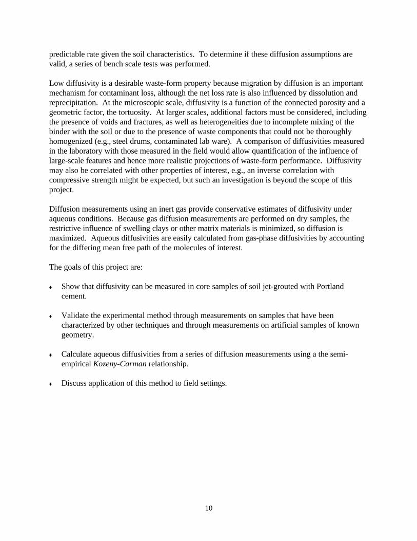
The goals of this project are:

♦ Show that diffusivity can be measured in core samples of soil jet-grouted with Portlandcement.

♦ Validate the experimental method through measurements on samples that have beencharacterized by other techniques and through measurements on artificial samples of knowngeometry.

♦ Calculate aqueous diffusivities from a series of diffusion measurements using a the semi-empirical Kozeny-Carman relationship.

♦ Discuss application of this method to field settings.

11

Experimental Apparatus

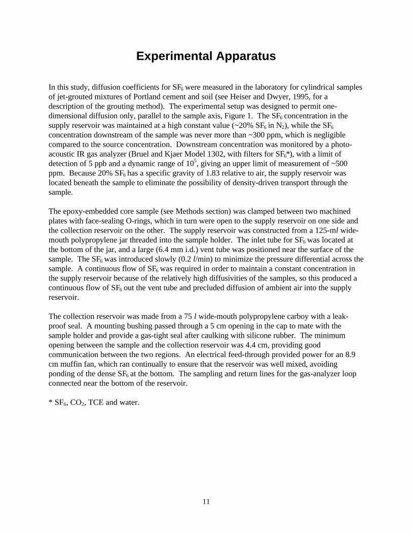
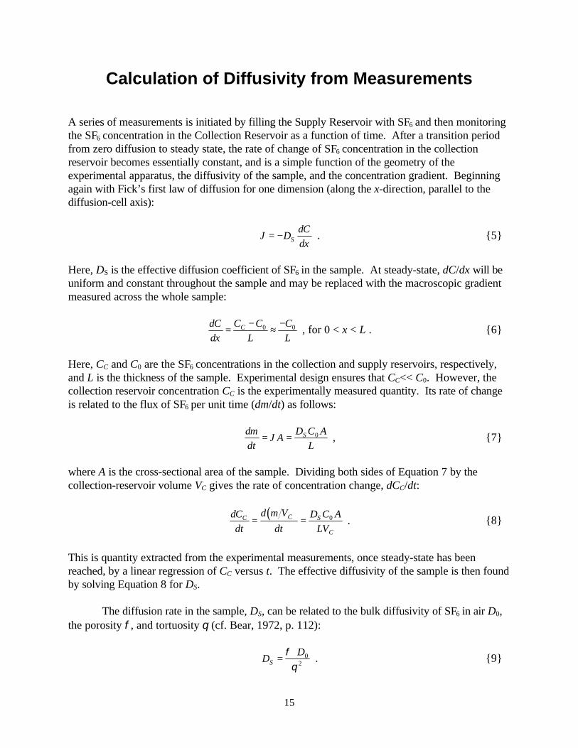
In this study, diffusion coefficients for SF6 were measured in the laboratory for cylindrical samplesof jet-grouted mixtures of Portland cement and soil (see Heiser and Dwyer, 1995, for adescription of the grouting method). The experimental setup was designed to permit one-dimensional diffusion only, parallel to the sample axis, Figure 1. The SF6 concentration in thesupply reservoir was maintained at a high constant value (~20% SF6 in N2), while the SF6

concentration downstream of the sample was never more than ~300 ppm, which is negligiblecompared to the source concentration. Downstream concentration was monitored by a photo-acoustic IR gas analyzer (Bruel and Kjaer Model 1302, with filters for SF6*), with a limit ofdetection of 5 ppb and a dynamic range of 105, giving an upper limit of measurement of ~500ppm. Because 20% SF6 has a specific gravity of 1.83 relative to air, the supply reservoir waslocated beneath the sample to eliminate the possibility of density-driven transport through thesample.

The epoxy-embedded core sample (see Methods section) was clamped between two machinedplates with face-sealing O-rings, which in turn were open to the supply reservoir on one side andthe collection reservoir on the other. The supply reservoir was constructed from a 125-ml wide-mouth polypropylene jar threaded into the sample holder. The inlet tube for SF6 was located atthe bottom of the jar, and a large (6.4 mm i.d.) vent tube was positioned near the surface of thesample. The SF6 was introduced slowly (0.2 l/min) to minimize the pressure differential across thesample. A continuous flow of SF6 was required in order to maintain a constant concentration inthe supply reservoir because of the relatively high diffusivities of the samples, so this produced acontinuous flow of SF6 out the vent tube and precluded diffusion of ambient air into the supplyreservoir.

The collection reservoir was made from a 75 l wide-mouth polypropylene carboy with a leak-proof seal. A mounting bushing passed through a 5 cm opening in the cap to mate with thesample holder and provide a gas-tight seal after caulking with silicone rubber. The minimumopening between the sample and the collection reservoir was 4.4 cm, providing goodcommunication between the two regions. An electrical feed-through provided power for an 8.9cm muffin fan, which ran continually to ensure that the reservoir was well mixed, avoidingponding of the dense SF6 at the bottom. The sampling and return lines for the gas-analyzer loopconnected near the bottom of the reservoir.

* SF6, CO2, TCE and water.

12

SF6 Supply @ 0.2 l/min(20% SF 6 in N 2)

Collector Reservoir(85 l)

SupplyReservoir(125 m l)

Mixing Fan

Sample

Vent (6.4 mm i.d.)

Pressure Equalizer(4.6 m x 6.4 mm

(length x i.d.))

Analyzer &Data Logger

XXX ppm

Figure 1. Diffusion cell.

13

A pressure-equalizing line connected the two reservoirs to ensure identical pressure in both, andhence zero pressure gradient across the sample. This line was 4.6 m long x 6.4 mm i.d., sufficientlength so that diffusion was negligible during the measurement period. This was verified bycalculating the rate of diffusion at steady-state. Beginning from Fick’s first law of diffusion forsteady-state conditions:

J DClpe

= 00 , {1}

where J is the flux into the reservoir per unit cross-sectional area of the tube, D0 is the diffusion

coefficient, C0 is the supply concentration (assumed to be constant at 2·105 ppm SF6), and lpe isthe length of the pressure-equalizing tubing. The concentration gradient is thus C0/lpe, with theimplicit assumption that the concentration in the collection reservoir is negligible in comparison toC0. A tube of diameter d will have a cross-sectional area of πd2/4, so the flux of mass m per unittime t into the reservoir will be:

dmdt

Jd

=π 2

4 . {2}

Dividing by the volume of the collection reservoir, VC, gives:

14

2

Vdmdt

d mV

dtJ d

VR

C

R

⋅ =

=π

. {3}

The concentration in the collection reservoir (CC) is mass per unit volume, corresponding to m/VR

here, and J may be expanded using Equation 1 to give:

dCdt

D C dl V

C

pe C

= 0 02

4π

, {4}

which is the rate of change of concentration of SF6 in the collection reservoir. The diffusioncoefficient, D0, is the only variable on the right-hand side that is not a function of the experimentalsetup. As a conservative proxy for D0, the average diffusion coefficient for various gases into airwas used (0.13 cm2/s, Weast, 1973). Because of its size and mass, SF6 must diffuse substantiallymore slowly. For a reservoir volume (VC) of 85 l, tubing inside diameter (d) of 6.4 mm, andtubing length (lpe) of 4.6 m, the calculated rate of increase of SF6 in the collection reservoir is0.013 ppm/min. This value is negligible in comparison to values from actual diffusion experiments(~5 ppm/min), and suggests that diffusion through the pressure-equalizing line may be safelyignored.

Less easily dismissed is the possible role of air pressure fluctuations driving SF6 from the supplyreservoir through the pressure-equalization tube to the collection reservoir. The experimentswere performed in a laboratory located in a large modern four-story (+ basement) building withsealed windows and central heating and air conditioning. As the ventilation equipment cycled onand off, the building was pressurized and de-pressurized slightly. These pressure changes musthave engendered some flow through the pressure-equalization line, lasting until equilibrium was

14

re-established. An increase in ambient pressure would have caused flow from the supply to thecollection reservoir, resulting in a step-like increase in measured SF6 concentration. A decrease inambient pressure was less problematic, causing flow from the collection to the supply reservoir,resulting in a short-term dilution of the supply gas. This would have lasted only a few minutesuntil the supply reservoir was replenished by the continuous flow of SF6. Much of the scatterobserved in the measurements is probably attributable to such air pressure variations.Measurements made during weekends when the building ventilation was shut down wereessentially noise-free.

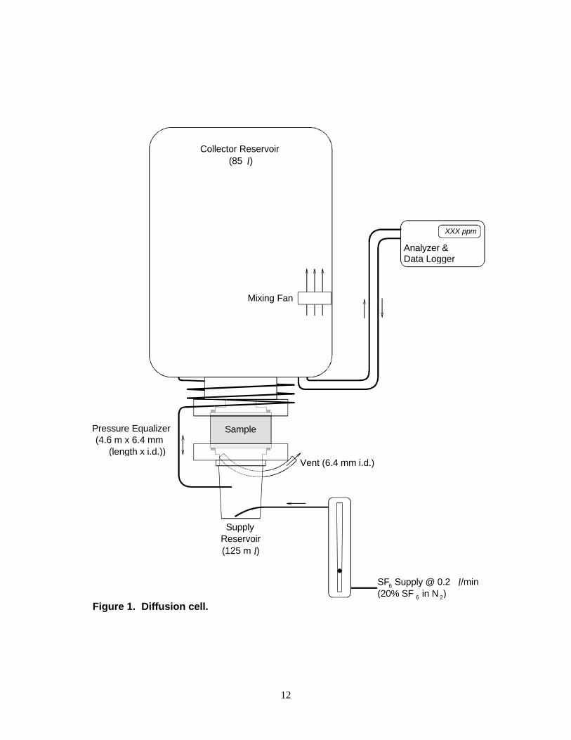
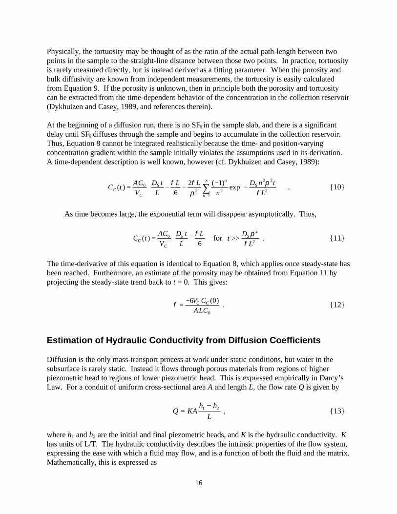
Measurements were also made employing the alternate geometry for pressure equalizationillustrated in Figure 2. Here, the pressure-equalization tubes from each reservoir were open to theambient laboratory atmosphere. Calculations using Equation 4 show that SF6 loss from the supplyreservoir due to diffusion through the pressure-equalization tube was negligible at ~0.1%/h, andwas two orders of magnitude less for the collection reservoir. To eliminate turbulence and anypressure differential, the SF6 flow (0.2 l/min) into the sample reservoir was turned off after threeminutes, and the vent was plugged. Thus the supply reservoir was completely static once it hadbeen filled, so there was no gas motion across the supply-side of the sample. Additionally,fluctuations in ambient pressure could not have induced transport of SF6 through the pressure-equalization lines because they no longer provided a direct link from the supply to the collectionreservoirs. Changes in ambient pressure still played a role, however, because the two reservoirsprobably did not equilibrate at the same rate, which led to transient pressure gradients across thesample. This in turn showed up as noise in the concentration profile versus time for the collectionreservoir.

SupplyReservoir(250 m l)

Sample

Vent (plugged)

Pressure Equalizer(2 m x 6.4 mm(length x i.d.))

Pressure Equalizer(40 cm x 1.6 mm

(length x i.d.))SF6 (off)

Sampling port

Figure 2. Alternate geometry for the diffusion cell.

15

Calculation of Diffusivity from Measurements

A series of measurements is initiated by filling the Supply Reservoir with SF6 and then monitoringthe SF6 concentration in the Collection Reservoir as a function of time. After a transition periodfrom zero diffusion to steady state, the rate of change of SF6 concentration in the collectionreservoir becomes essentially constant, and is a simple function of the geometry of theexperimental apparatus, the diffusivity of the sample, and the concentration gradient. Beginningagain with Fick’s first law of diffusion for one dimension (along the x-direction, parallel to thediffusion-cell axis):

J DdCdxS= − . {5}

Here, DS is the effective diffusion coefficient of SF6 in the sample. At steady-state, dC/dx will beuniform and constant throughout the sample and may be replaced with the macroscopic gradientmeasured across the whole sample:

dCdx

C CL

CL

C=−

≈−0 0 , for 0 < x < L . {6}

Here, CC and C0 are the SF6 concentrations in the collection and supply reservoirs, respectively,and L is the thickness of the sample. Experimental design ensures that CC<< C0. However, thecollection reservoir concentration CC is the experimentally measured quantity. Its rate of changeis related to the flux of SF6 per unit time (dm/dt) as follows:

dmdt

J AD C A

LS= = 0 , {7}

where A is the cross-sectional area of the sample. Dividing both sides of Equation 7 by thecollection-reservoir volume VC gives the rate of concentration change, dCC/dt:

( )dCdt

d m V

dtD C A

LVC C S

C

= = 0 . {8}

This is quantity extracted from the experimental measurements, once steady-state has beenreached, by a linear regression of CC versus t. The effective diffusivity of the sample is then foundby solving Equation 8 for DS.

The diffusion rate in the sample, DS, can be related to the bulk diffusivity of SF6 in air D0,the porosity φ, and tortuosity θ (cf. Bear, 1972, p. 112):

DD

S =⋅φθ

02 . {9}

16

Physically, the tortuosity may be thought of as the ratio of the actual path-length between twopoints in the sample to the straight-line distance between those two points. In practice, tortuosityis rarely measured directly, but is instead derived as a fitting parameter. When the porosity andbulk diffusivity are known from independent measurements, the tortuosity is easily calculatedfrom Equation 9. If the porosity is unknown, then in principle both the porosity and tortuositycan be extracted from the time-dependent behavior of the concentration in the collection reservoir(Dykhuizen and Casey, 1989, and references therein).

At the beginning of a diffusion run, there is no SF6 in the sample slab, and there is a significantdelay until SF6 diffuses through the sample and begins to accumulate in the collection reservoir.Thus, Equation 8 cannot be integrated realistically because the time- and position-varyingconcentration gradient within the sample initially violates the assumptions used in its derivation.A time-dependent description is well known, however (cf. Dykhuizen and Casey, 1989):

C tACV

D tL

L Ln

D n tLC

C

Sn

S

n

( )( )

exp= − − − −

=

∞

∑02 2

2 2

216

2 1φ φπ

πφ

. {10}

As time becomes large, the exponential term will disappear asymptotically. Thus,

C tACV

D tL

LC

C

S( ) = −

0

6φ

for tD

LS>>

πφ

2

2 . {11}

The time-derivative of this equation is identical to Equation 8, which applies once steady-state hasbeen reached. Furthermore, an estimate of the porosity may be obtained from Equation 11 byprojecting the steady-state trend back to t = 0. This gives:

φ =−6 0

0

V CALC

C C ( ) . {12}

Estimation of Hydraulic Conductivity from Diffusion Coefficients

Diffusion is the only mass-transport process at work under static conditions, but water in thesubsurface is rarely static. Instead it flows through porous materials from regions of higherpiezometric head to regions of lower piezometric head. This is expressed empirically in Darcy’sLaw. For a conduit of uniform cross-sectional area A and length L, the flow rate Q is given by

Q KAh h

L=

−1 2 , {13}

where h1 and h2 are the initial and final piezometric heads, and K is the hydraulic conductivity. Khas units of L/T. The hydraulic conductivity describes the intrinsic properties of the flow system,expressing the ease with which a fluid may flow, and is a function of both the fluid and the matrix.Mathematically, this is expressed as

17

K = kρg/µ , {14}

where k is the permeability of the matrix, ρ is the density of the fluid, g is the acceleration due togravity, and µ is the dynamic viscosity of the fluid. The permeability, with units of L2, dependsonly upon the matrix and is independent of the properties of the fluid. Thus if permeabilities canbe estimated from diffusion measurements, hydraulic conductivities can be calculated fromEquation 14 and knowledge of the fluid properties.

A number of empirical relationships between permeability and various geometrical properties ofporous media have been proposed (cf. Bear, 1972). These include terms such as effective grainsize and various shape factors, and were derived to predict permeability in granular materialsranging from uniform spherical beads to poorly sorted angular sand grains. Applicability of suchrelationships to a non-granular matrix such as Portland cement is dubious at best, in part becauseit is unclear how the empirical fitting parameters should be measured in such a material.

The alternative is to proceed from a theoretical basis to arrive at a general expression for thepermeability in terms of a few clearly defined physical properties. This has not been entirelyachieved, but the Kozeny-Carman equation comes close, predicting permeabilities based on thesurface area, porosity, tortuosity, and Kozeny’s constant, which depends upon the geometry ofthe pores. Derivation of the Kozeny-Carman equation is outlined in Bear (1972). Briefly, theporous medium is considered to be a bundle of capillaries of equal length. Flow through a singlecapillary of circular cross-section is governed by Poisseuille’s law, and non-circular cross-sectionsare accounted for by the introduction of a shape factor that can be calculated for simplegeometries. The size of the capillaries leads to the concept of the hydraulic radius, defined as theratio between cross-sectional area and wetted-perimeter length. The hydraulic radius is alsomeasured by the ratio of porosity to surface area. By solving the Navier-Stokes equations forflow through all channels penetrating a cross-section normal to the flow direction, Kozeny wasable to derive an expression for the permeability in terms of intrinsic matrix properties:

( )k c

Asp m

=−

03

21

θ φφ ρ

. {15}

Here, c0 is Kozeny’s constant, Asp is the specific surface area per unit mass, and ρm is the densityof the non-porous solid matrix.

Carman’s empirical studies showed that c0θ = 15 gave good agreement with experimental data,

giving rise to the Kozeny-Carman equation:

( )k

Asp m

=−

φφ ρ

3

25 1

. {16}

Carman’s experimental data was almost certainly obtained from measurements on granularporous media, so once again the question of applicability to Portland cement arises. It seems

18

likely that a cementitious material will have a much different pore geometry than a granularmaterial, probably leading to c0θ ≠ 1

5 . A comparison of predicted and measured permeabilitiesmay resolve this question.

19

Experimental Methods

Sample Preparation and Descriptions

A total of four core samples of jet-grouted Portland cement were obtained from the LandfillDemonstration Area in Tech Area 3 at Sandia National Laboratories. The grout was emplaced aspart of a demonstration project, described in Allan and Kukacka (1994). Duplicate samples wereobtained from two groutings ~75 cm in diameter by ~1 m high, which were part of an array of testgroutings. The sample designated P36-1 was in place, but its exact location in the array isunknown because a pit only 1 m × 2 m was excavated. P36-2 was out of place, found at the edgeof the excavation, but was known to have been located at the northeast corner of the arrayoriginally.

A detailed discussion of the composition of some of the test groutings is reported in Allan andKukacka (1995). They report that the jet-grouted cement was a mixture of soil, cement, slag (inone test grouting), water, bentonite, and a “superplasticizer”, giving a cementitious content of 16–26%. Soil in this area is a poorly-sorted sandy loam with occasional gravel-size rock fragments.The cured grout contains only faint flow-banding indicating nearly complete homogenization ofthe soil and cement. Allan and Kukacka report bulk densities ranging from 1.70 to 1.95.

The samples were cored in-situ from the test groutings using a hand-held industrial drill with a10.16 cm (4 in) outside-diameter coring bit cooled with water. The extracted cores had adiameter of ~8.9 cm (3.5 in). The core samples were cleaned ultrasonically in deionized water for20 min, rinsed in deionized water, and allowed to dry. Later, the ends were squared off with awater-cooled slab saw and then scrubbed with a brush under running tapwater and finally air-driedfor at least one week before further treatment. When wet after each washing, the cores smelledstrongly of Portland cement, suggesting that the grout may still be quite reactive chemically. Theimplications of this have not been investigated further.

The purpose of the various washing procedures was to remove all cutting debris that mightotherwise reduce the permeability of the sample. The coring operation produced a lot of clay-sizematerial which caked on the core surface. Ultrasonic cleaning removed most of this, but a goodscrubbing would probably have been just as effective. The slab-saw cooling water also containeda lot of clay-size fines, but no caking occurred. The cores were scrubbed until no further loss offines was evident visually, a process which required only a minute or so. Although deionizedwater was used for the ultrasonic wash, tapwater would have been adequate, as it was for laterwashing.

The cores were prepared for diffusion measurements. Casting in plastic (polyester resin[Plasticare Casting Resin] or epoxy resin [Shell Chemical Co. EPON 828 resin and Epi-Cure 3055curing agent]). The encapsulated cores were sectioned using the slab saw to obtain a ~5 cm thicksample perpendicular to their axes. After sectioning, saw marks were polished out using a lapwheel with self-adhesive 120 grit SiC abrasive paper and tapwater.

20

Two casting methods were tested. In the first, an 11.43 cm (4.5 in) outside-diameter acrylic tubewas used as a “consumable” form — it was left in-place after the resin cured, becoming anintegral part of the sample holder. This proved troublesome. Polyester resin adhered strongly tothe acrylic but only weakly to the sample. As the resin contracted upon curing, it pulled awayfrom the core, opening a channel along the surface of the core. Epoxy resin formed a strong bondwith the core but adhered only weakly to the acrylic tube, partially separating at this surfaceduring sectioning and subsequent handling.

In the second casting method, a 12.06 cm (4.75 in) inside-diameter acrylic tube was used as areusable form by coating its inside surface with a release agent (silicone high-vacuum grease forpolyester resin, Miller-Stephenson TFE release agent for epoxy resin). This method worked wellwith both resins, but there appeared in places to be a thin film of air at the interface between thecore and the polyester resin. As the film did not appear to be continuous, the sample (36-1a) wasnot recast. The epoxy formed a strong bond with the core and released easily from the form whenthe form was tapped with a soft mallet.

The epoxy-resin reusable-form casting method was superior. The epoxy exhibited negligibleshrinkage, bonding well to the core, yet released easily from the mold using a clean easily appliedrelease agent. It cured relatively slowly, however, and thus penetrated any fractures present. Ifthe fractures connected with voids, these too became filled with epoxy. The epoxy did not appearto penetrate deeply into the grout itself, seeping only ~2 mm into the matrix from the edge of thecore or any fracture surface. The curing reaction is exothermic, and can lead to significanttemperature increases (maximum temperatures exceeding 100 °C in some cases) when castinglarge (>300 ml) volumes. To facilitate mixing, the resin was warmed to 60 °C before combiningwith the curing agent (at 25 °C), and had a pot-life of 20–30 min before heat generated by curingbegan to raise the temperature and accelerate the curing rate. This run-away condition did notoccur once the epoxy was poured into the annulus surrounding the core sample in the castingform. Vacuum-degassing of the mixed epoxy was evaluated and found to be unnecessary. Only afew bubbles adhered to the sample or the walls of the form, while any suspended bubbles floatedto the surface before curing was complete. The number of bubbles was not significantly reducedby ~15 min of degassing (longer degassing was not practical due to limited pot-life).

Polyester resin offers several advantages over epoxy if sample-adhesion could be improved. Withthe addition of the appropriate amount of catalyst, curing times can be much shorter, leading tomuch less penetration of fractures and voids. This would permit more realistic estimates of thebulk properties of the sample rather than focusing on the matrix. The polyester resin is alsowater-clear instead of dark translucent olive green. The casting process for either resin could beimproved if the sample could be wrapped or coated with some material that would preventimpregnation but would not hamper adhesion. Another alternative might be to use an acrylicresin. Some acrylics cure very quickly (~5 min) and thus may not penetrate very deeply intofractures. They also exhibit low shrinkage. They are opaque, however, so quality of adhesion tothe core would be difficult to verify visually, and open channels might not be detected untildiffusion measurements were made.

21

Individual samples are summarized in Table 1. The suffixes a and b distinguish among duplicatesamples from the same test grouting. Dimensions of the prepared samples were measured usingdigital calipers. The quoted diameter is an average value of the minimum and maximum diametersof the top and bottom surfaces, and the range is the difference between the smallest and largestmeasured diameters. The quoted height is an average of the minimum and maximum heights, andthe range is the difference between the minimum and maximum heights. Void space and clastfractions on the top and bottom surfaces were estimated visually (top and bottom are with respectto the orientations of the cores as sampled from the Chemical Waste Landfill DemonstrationArea).

Table 1. Sample descriptions.

Sample Casting MethodDimensions (mm);Top, Bottom (%) Comments

36-1a Resin: PolyesterForm: Removable

Diameter: 94.5Range: ±0.1Height: 51.2Range: ±0.9

Voids: <1%, 2%Clasts: 10%, 15%

Slight separation of the resin from the core nearthe top and bottom, possible connectedpathway from top to bottom. One void on thebottom extends several centimeters into thesample.

36-1b Resin: EpoxyForm: Integral

Diameter: 94.4Range: ±0.1Height: 50.8Range: ±0.6

Voids: 2%, 2%Clasts: 3%, 10%

Partial separation at acrylic/epoxy interface, butno connected pathway from top to bottom, andthis area is outside of seal so will not see SF6.Six hairline fractures are visible on the topsurface; only three on the bottom. A large clast(3 cm x 2 cm) is exposed on the bottom.

36-2a Resin: EpoxyForm: Removable

Diameter: 94.6Range: ±0.2Height: 47.8Range: ±0.7

Voids: 7%, 7%Clasts: 3%, 5%

Was first cast using polyester resin, butadhesion was poor so old resin was chipped off.Voids are numerous and small (usually < 3mm). Soil clots were not counted as clasts, astheir porosity is high. Few were present on thetop, but they constituted ~3% of the bottom.Several small fractures oriented radially fromthe edges are filled with epoxy, but there is nogeneral impregnation.

36-2b Resin: EpoxyForm: Removable

Diameter: 94.4Range: ±0.6Height: 46.2Range: ±1.2

Voids: 5%, 4%Clasts: 7%, 4%

Contains a fracture parallel to the axis of thecore. The fracture and several large voidsbecame filled by epoxy during casting, and werecounted as clasts.

22

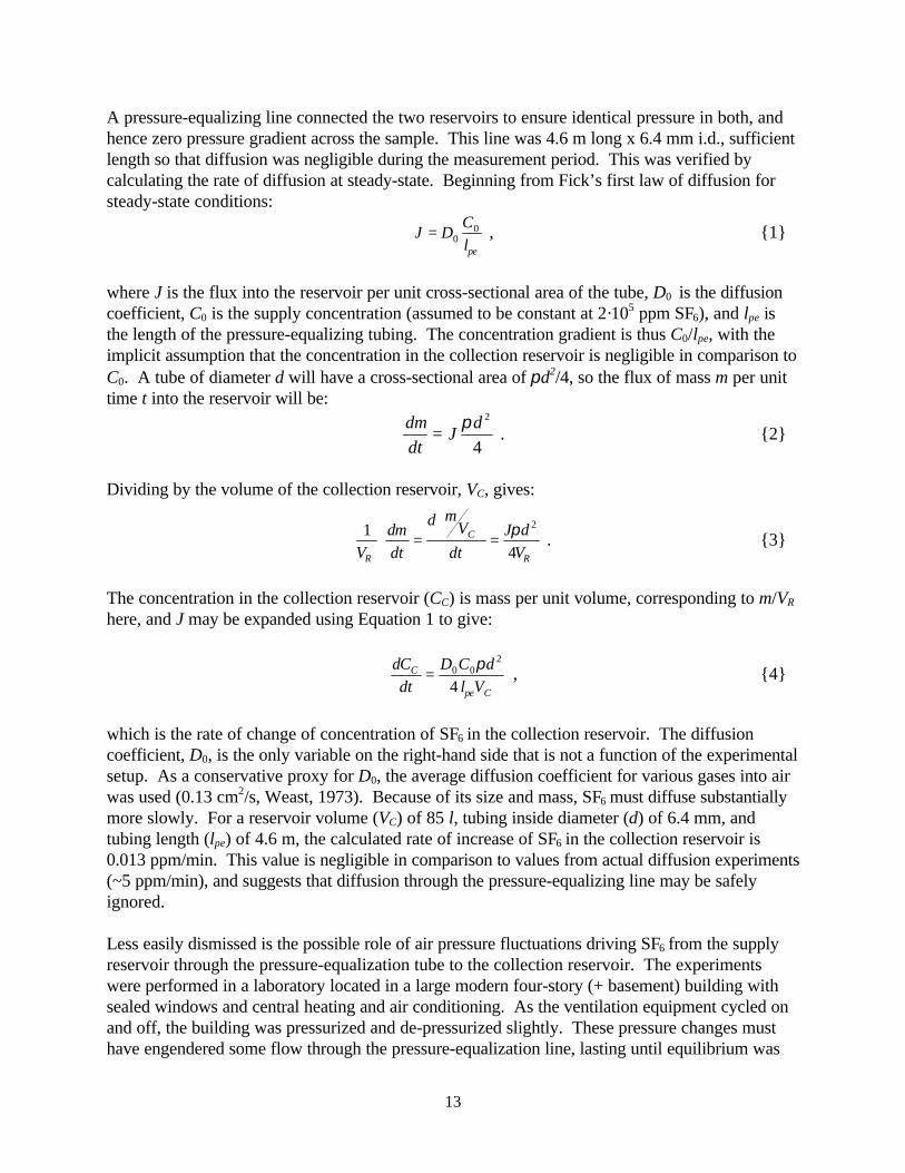
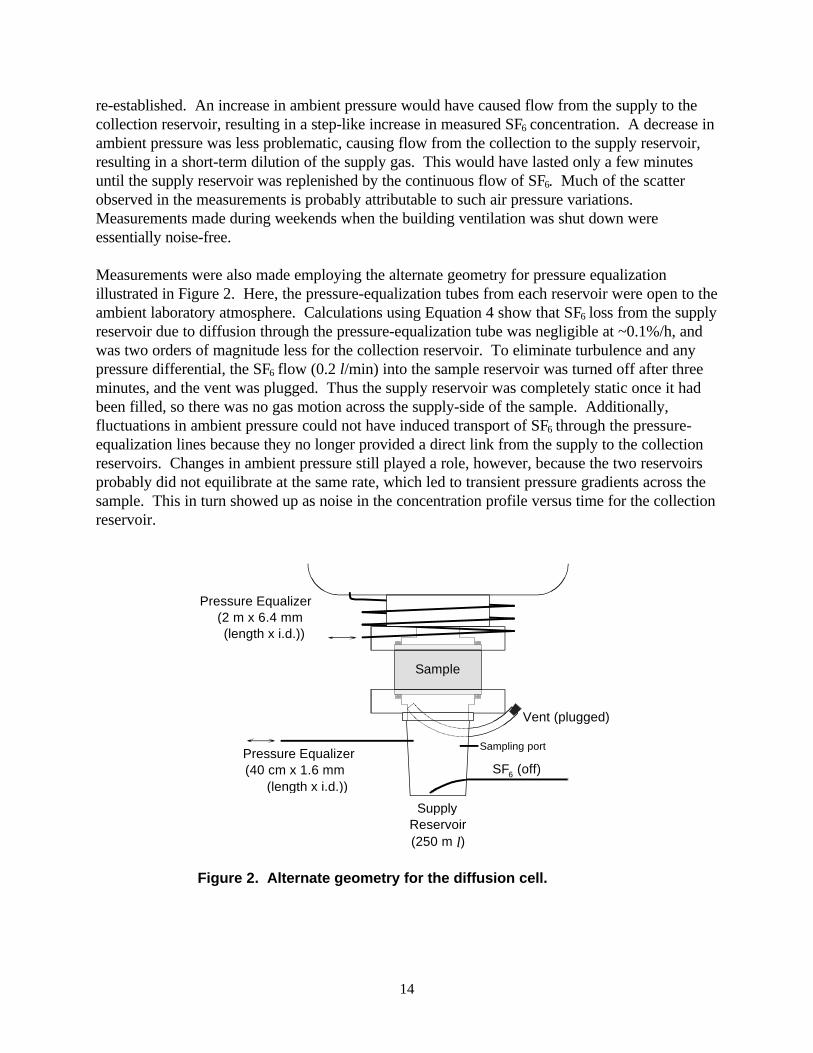
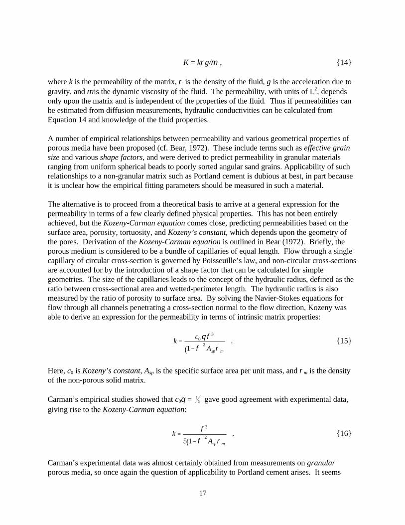
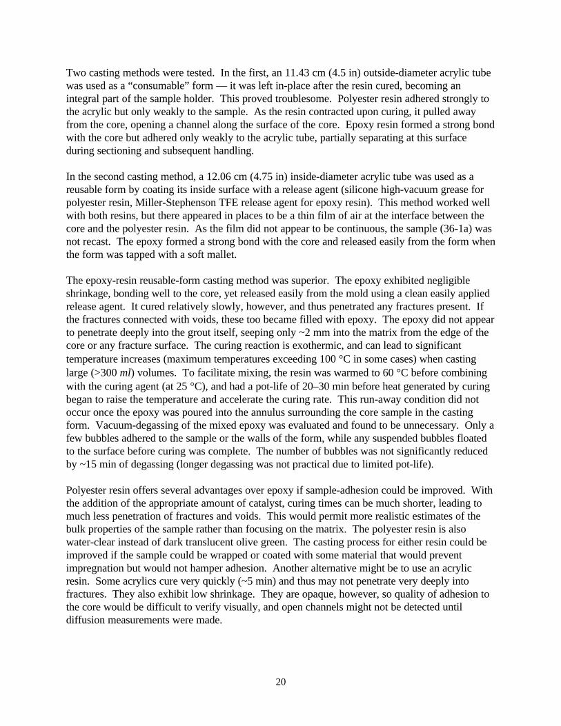
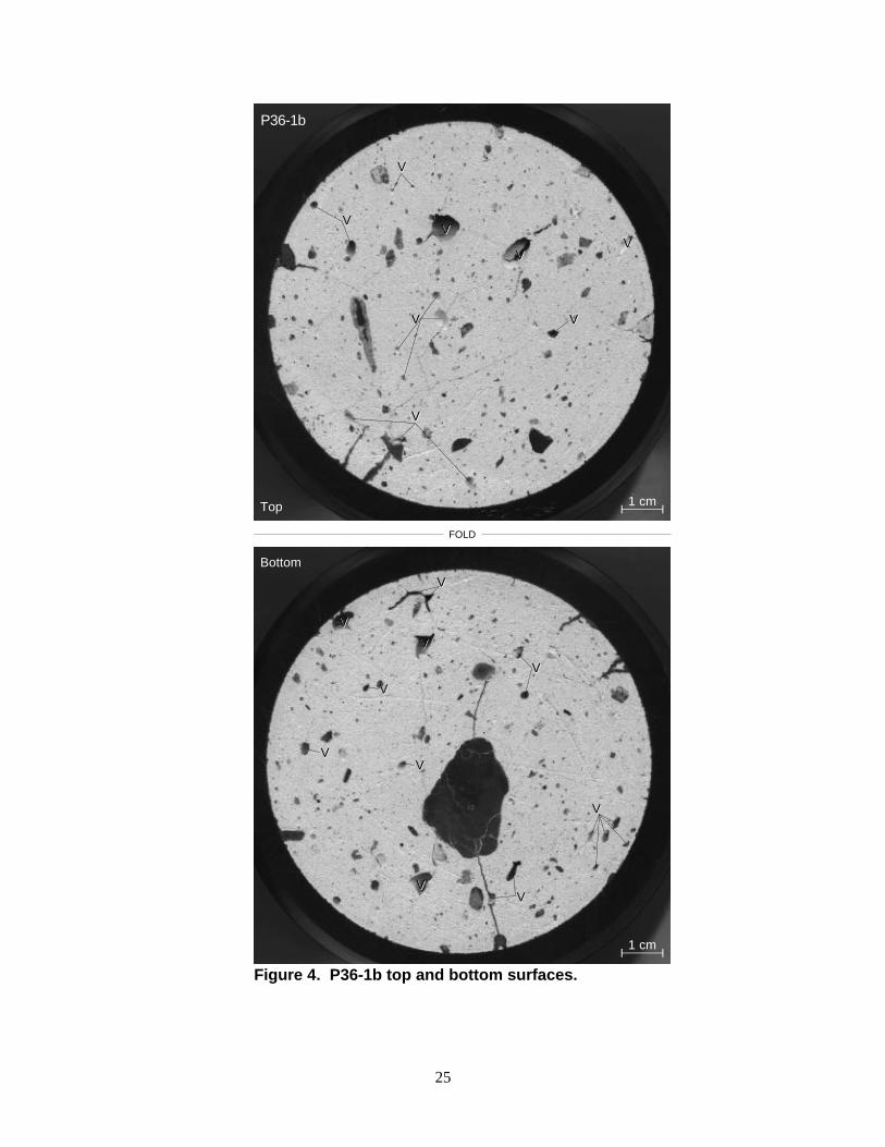
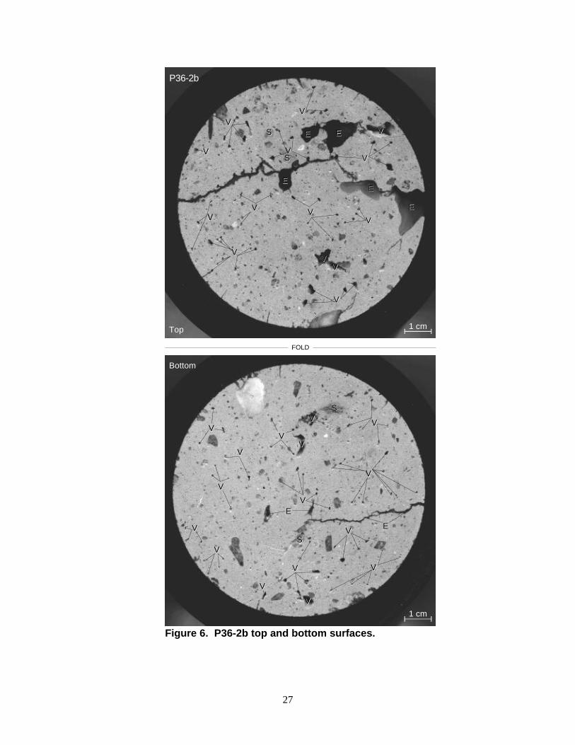
In the following images of the top and bottom surfaces of each prepared core sample (Figures 3–6), large voids are overlaid with a “V”, and smaller voids (> 0.5 mm) are indicated by linesconnecting them to a “V”. Dark clasts without labels are rock fragments. Lighter clasts labeled“S” are clots of indurated soil. In several places, the epoxy seeped along fractures and filledadjoining voids. These features have been labeled with “E”.

The top and bottom surfaces of P36-1a are shown in the images in Figure 3. Rock fragments areabundant, and are predominantly feldspar, quartz, and fine-grained metamorphic rocks derivedfrom weathering of the nearby Manzano Mountains. These lithologies have little porosity and willact as barriers to diffusion. Two lighter-colored clasts labeled “C” are also present on the topsurface, and appear to be fragments of Portland cement; one of these contains small rockfragments of the same lithology as described above. There are only a few shallow voids on thetop surface, but two large voids on the bottom significantly penetrate the sample. The void at 1o’clock is 2 cm deep and extends laterally beneath the surface for 1 cm towards the axis of thesample. The other large void, at 3 o’clock, is approximately 1 cm deep and no wider than whereit intersects the surface. Linear features visible on both surfaces are artifacts of the polishingprocess. Slight flow-banding may be discerned on the top surface. This sample was cast inpolyester resin using the removable form. The resin separated slightly from the core near the topand bottom, as evidenced by a reflective film of air between the resin and the core which indicatedthat a connected pathway may extend from top to bottom over ~25% of the circumference.

As may be seen in Figure 4, P36-1b differs slightly from P36-1a, containing fewer rock fragmentsbut slightly more medium-size voids (<5 mm). Larger voids are also present on each surface,significantly penetrating the sample up to 1 cm. A large clast (3 cm x 2 cm) is exposed on thebottom. The most critical difference may be the network of hairline fractures evident on the topand bottom surfaces, which may provide low-tortuosity paths for SF6 diffusion. Linear featuresvisible on both surfaces are artifacts of the polishing process. This sample was cast in epoxy usingan integral acrylic form. Partial separation occurred at the acrylic/epoxy interface, but noconnected pathway extends from top to bottom, and this area is outside of the seal so will not besubjected to SF6.

The top and bottom surfaces of P36-2a are shown in Figure 5. The cement matrix is gray ratherthan nearly white as it is in the P36-1 samples. Rock fragments are not very numerous, but thereare several clots of indurated sand, labeled with “S”. Although there are no large voids on the topsurface, there are numerous smaller ones, most of which penetrate beyond visual range (>3–5mm). The bottom surface is even more riddled with voids, and contains several large ones, ~1 cmacross. Some of these appear to be cavities remaining from sand clots that were disaggregatedand washed away during cutting and washing. A fracture on the bottom surface at 5 o’clockpenetrates several centimeters into the sample and was filled with epoxy during casting, as wereseveral other smaller fractures visible around the edges of this surface. There is no generalimpregnation of the sample by the epoxy. This sample was first cast using polyester resin, butadhesion was poor so the resin was chipped off, and the sample was recast using epoxy and theremovable form. The epoxy bonded well to the sample surface, leaving no air channels.

23

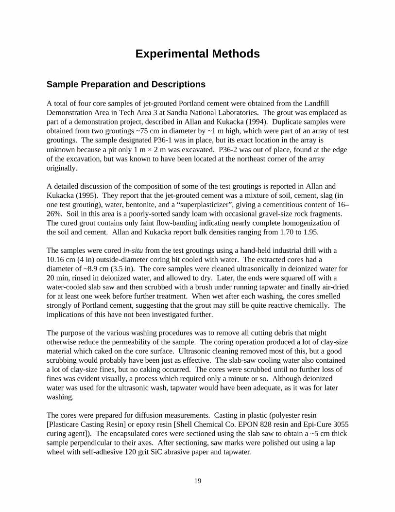
As may be seen in Figure 6, the cement matrix of P36-2b is very similar to that of P36-2a in termsof the distribution of small voids, rock fragments, and soil clots. The distinguishing feature of thissample is a fracture and several associated voids that cuts across the top surface. During casting,epoxy seeped along this fracture and filled the adjoining voids, but did not impregnate the cementmatrix. On the bottom surface, this fracture only penetrates halfway across the sample. Theplane of the fracture appears to be approximately parallel to the axis of the sample. This samplewas cast in epoxy using the removable form; the epoxy bonded well to the sample surface, leavingno air channels.

24

VV

VVVV

VV

VV

VV

VV

VV

VV

VV

VV

FOLD

Bottom

Top

P36-1a

1 cm

1 cm

CC

CC

Figure 3. P36-1a top and bottom surfaces.

25

VV

VV

VV

VV

VV

VV

VVVV

VV

VV

VV

FOLD

Bottom

Top

P36-1b

VV

VV

VV

VV

VV

VV

VV

1 cm

1 cm

Figure 4. P36-1b top and bottom surfaces.

26

VV

VV

VV

VV

VV VV

VV

VV

FOLD

Bottom

Top

P36-2a

VV

VV

VV

VV

VV

VV

VVVV

VV

VV

VV

VV

VV

VV

VVVV

1 cm

1 cm

SS

SS

SS

SSSS

SS

SS

SS

SS

SS

EE

EE

EE

Figure 5. P36-2a top and bottom surfaces.

27

VV

VV

VV

VV

VV

FOLD

Bottom

Top

P36-2b

VV

VV

EE

EE

EE

EE

EE

VV

VV

VV

VV

VV

VV

VV

VV

VV

VV

VV

VV

VV

VVVV

VV

VV

VV

VV

VV

VV

EE

EE

1 cm

1 cm

SS

SS

SS

SSVV

Figure 6. P36-2b top and bottom surfaces.

28

Surface Area Determinations

All surface areas were measured by N2-BET using a fully automated Micromeritics ASAP 2000following standard methods. The end pieces that were cut from each core sample were lightlycrushed, and a few grams of chips (≤ 5 mm in longest dimension) were hand-picked for surface-area analysis, avoiding clasts. Samples were degassed overnight (15–23 h) at 50°C beforeanalysis. Higher temperatures would have risked excessive loss of water from the cement gel(cf. Lea, 1971) Replicate analyses differed by less than 1%, even after an additional 7 h ofdegassing.

Diffusion Measurement Protocol

Instrument Operation

The Bruel and Kjaer Model 1302 photo-acoustic gas analyzer was configured with the followingfilters in addition to the standard water vapor filter (gas and detection limits in parentheses): UA0936 (SF6 0.7 ppm), UA 0978 (trichloroethylene), UA 0983 (CO2 1.7 ppm), and UA 0988 (SF6

0.005 ppm). Measurements for SF6 were performed using UA 0988 with interference correctionsfor trichloroethylene, CO2, and water vapor. An MS-DOS personal computer was used as a datalogger, running the software supplied with the instrument and connected to the gas analyzer viaRS-232C serial ports. The instrument was configured using parameters of 626 mm Hg for thelocal air pressure (a typical value for Albuquerque), a temperature of 22.5°C, and an inlet tubelength of 1.92 m (1.68 m of 3.175 mm i.d. tubing was used, whereas the instrument wascalibrated for 3 mm i.d. tubing). The instrument was allowed to warm up by taking continuousreadings for at least 20 minutes before any measurements on samples or standards were made.The instrument was configured to measure continuously, with no delay between samples.Measurements were logged by attached computer and data reduction was performed later.

The gas analyzer was leased from Bruel and Kjaer in a fully calibrated condition. Calibration wasverified by running a 259 ppm SF6 standard in N2 before each measurement run, and the differencebetween the measured value and the nominal value was used as a normalizing factor to correctmeasurements on unknowns. Except for a two-day period of erratic behavior, readings werequite stable, with measured values for the 259 ppm standard ranging from 209 to 211 ppm over a14 day period. The difference between the nominal value and the measured values was due todeclining sensitivity near the upper end of the instrument’s measurement range. A calibrationcurve accounting for this was developed.

The standard gas was measured using two different methods. In the first, recommended by Brueland Kjaer, SF6 was vented through an open-ended line at 2 l/min. A tee 1 m from the endbranched to the gas analyzer, and a flow gauge downstream of the tee verified that positive flowwas maintained during sampling. In the second, a Tedlar gas-sampling bag was first evacuatedusing a 60 ml syringe, and then was filled with ~1 l of the standard gas. For analysis, the gasanalyzer was connected directly to the bag. Results of the two methods were indistinguishable.

29

Measurement of Samples Requiring Dilution

The concentration of the supply-reservoir gas (~20% SF6) could not be measured directly usingthe UA 0988 filter, but required a 1:1000 dilution. Also, development of a calibration curverequired a series of dilution of the 259 ppm standard gas. Dilutions were performedvolumetrically using a set of syringes with nominal volumes of 1, 5,10, 60, and 1000 ml. Actualvolumes were determined gravimetrically using water, and were precise to 0.005 ml or 0.1%,whichever was larger. Compressed air from the building’s physical plant was used as the diluent.The requisite volumes were mixed in a Tedlar gas-sampling bag that had first been evacuated byhand using a 60-ml syringe. Dilutions of the 259 ppm standard mixed readily with air, yieldingconsistent readings after gentle agitation. Dilutions of the 20% SF6 required more severe mixing— after both SF6 and air were injected into a Tedlar bag, an empty 60-ml syringe was attachedand rapidly cycled ten times. To reduce errors, all syringes were first “rinsed” several times withthe gas they were to be filled with before measuring the actual aliquots. For analysis, the gasanalyzer was connected directly to the bag.

Sample Diffusion Measurement

A series of measurements on a sample in the diffusion cell began with several minutes ofmonitoring to establish an accurate baseline before 20% SF6 was introduced into the supplyreservoir (the baseline was often greater than zero because of residual SF6 from previous runs).After the baseline was established, the time was noted and the SF6 flow was started at a rate of 0.2l/min, which was maintained throughout the measurement series (method 1, geometry as in Figure1), or was shut off after three minutes (method 2, alternate geometry as in Figure 2). In method2, a sample of the supply reservoir was taken two minutes after the SF6 was shut off. Monitoringcontinued until the SF6 concentration in the collection reservoir reached ~200 ppm. Then thesupply reservoir was sampled and diluted in duplicate and measured. Finally, one or morealiquots of the 259 ppm standard were measured.

The time associated with each measurement must be corrected for the time lag inherent in thesystem. The two most important lags are the time required to fill the supply reservoir, and thetime required to mix the collection reservoir. These are accounted for by a single offset, whichwas determined from a series of measurements on a solid disk with an orifice of ~8 mm dia. × ~27mm long. Regression of concentration vs. time yielded a time-intercept of 92 s for the 125 mlreservoir (method 1) or 134 s for the 250 ml reservoir (method 2).

30

Results

Measurements were made to determine a calibration curve for the gas analyzer, to constrainpossible values of the bulk diffusion constant for SF6 into air, and to determine diffusioncoefficients for SF6 through jet-grouted Portland cement. Surface area measurements were madeso that the diffusion coefficient could be related to hydraulic properties.

Surface Area Measurements

Surface area (Asp) measurements by N2-BET are listed in Table 2. Accuracy of the measurementsmay be estimated from deviation between nominal and measured values for the 10.9 m2/gstandard, which amounts to ~3%. Variation from sample to sample from the same groutingexceeds the variation between the two groutings. The cause of these variations is probably due tosmall sample size and lack of representativeness, and they indicate that extrapolations frommeasurements on a few chips to an entire cored sample may have an additional uncertainty of 6–8%.

Table 2. Surface areas by N2-BET.

Sample Asp (m2/g)

P36-1a 23.41P36-1b 27.34P36-2a 23.46P36-2b 20.41Standard

(10.9 m2/g)10.62

Calibration Curve

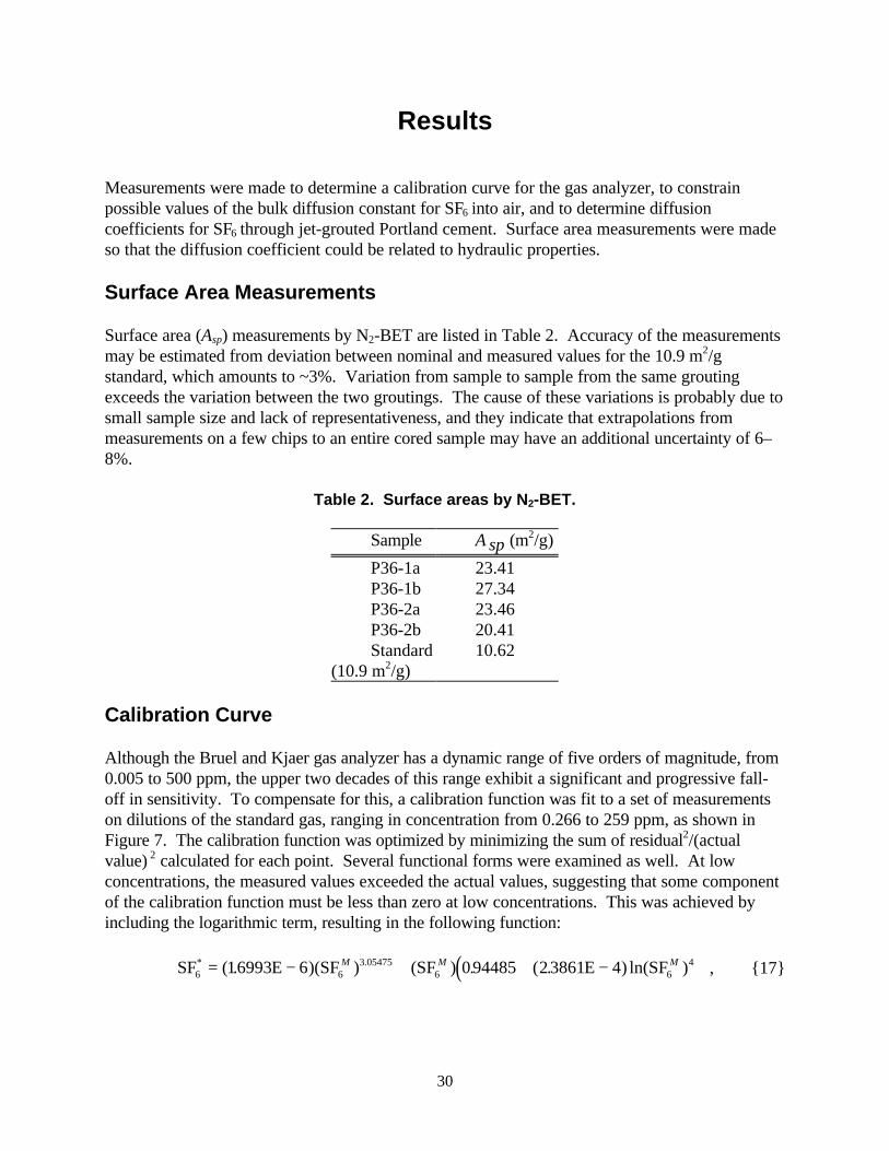
Although the Bruel and Kjaer gas analyzer has a dynamic range of five orders of magnitude, from0.005 to 500 ppm, the upper two decades of this range exhibit a significant and progressive fall-off in sensitivity. To compensate for this, a calibration function was fit to a set of measurementson dilutions of the standard gas, ranging in concentration from 0.266 to 259 ppm, as shown inFigure 7. The calibration function was optimized by minimizing the sum of residual2/(actualvalue) 2 calculated for each point. Several functional forms were examined as well. At lowconcentrations, the measured values exceeded the actual values, suggesting that some componentof the calibration function must be less than zero at low concentrations. This was achieved byincluding the logarithmic term, resulting in the following function:

( )SF E E6 63 05475

6 6416993 6 094485 23861 4* .( . )(SF ) (SF ) . ( . ) ln(SF )= − + + −M M M , {17}

31

where SF6M is the measured value and SF6

* is the corrected value. Except for the logarithmicterm, all terms are monotonically increasing, so the function can have at most one inflection point.Because this function cannot change direction to pass through each point, but instead must be asmooth curve, the magnitude of the residuals provides an estimate of the analytical precision ofthe measurements. Between 2 and 260 ppm, the residuals average less than ± 0.23% of themeasured values, suggesting that this aspect of the measurement process in an insignificant sourceof uncertainty.

After correcting for non-linear response, measurements were normalized according to aconcurrent measurement on the 259 ppm SF6 standard, SF6

* (259). This may be expressedmathematically as:

SF SFSF6 6

6

259259

N = ⋅** ( )

. {18}

Because of the stability of the gas analyzer, this final correction amounted to less than 0.5% in allcases.

32

0

50

100

150

200

250

300

0 50 100 150 200 250 300

Actual Concentration (ppm)

Mea

sure

d C

on

cen

trat

ion

(p

pm

)

Measurements

1:1 correlation l ine

Corrected values

x = 1 .6993E-06* y^3 .05475 + (0 .94485 + 2 .3861E-04* ln(y)^4)* y

SF6 Calibration Curve for B&K Gas Analyzer

Figure 7. Calibration curve for gas analyzer.

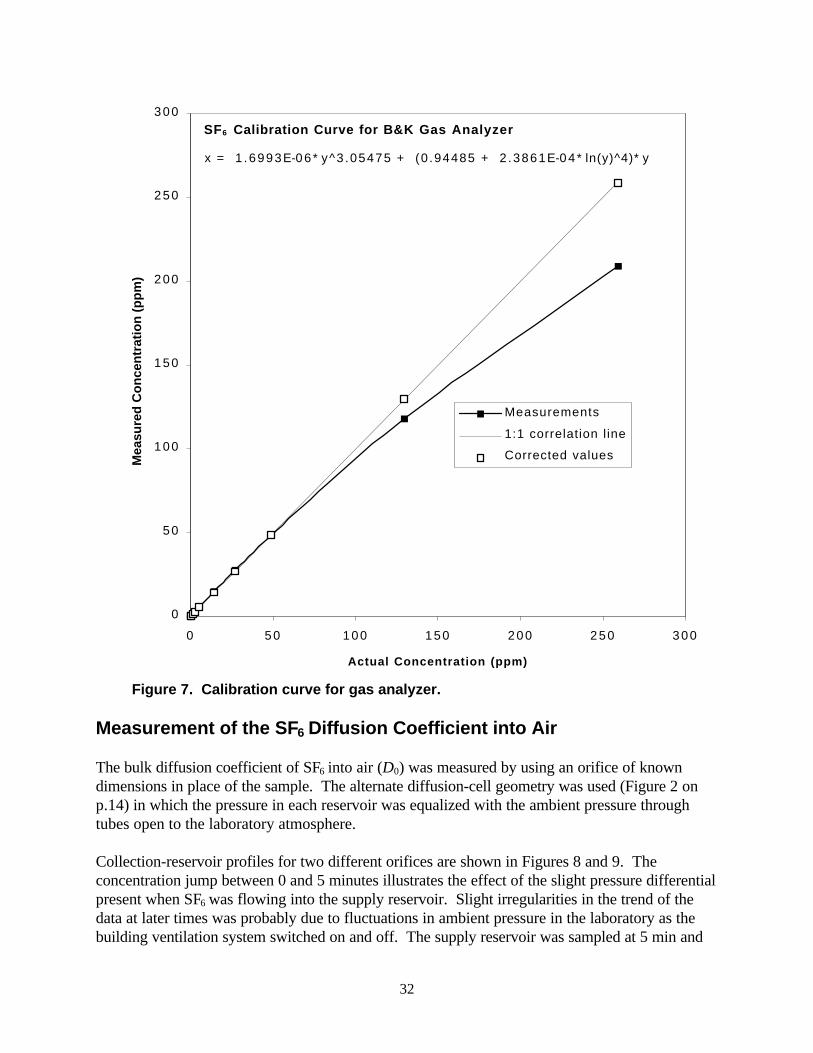
Measurement of the SF6 Diffusion Coefficient into Air

The bulk diffusion coefficient of SF6 into air (D0) was measured by using an orifice of knowndimensions in place of the sample. The alternate diffusion-cell geometry was used (Figure 2 onp.14) in which the pressure in each reservoir was equalized with the ambient pressure throughtubes open to the laboratory atmosphere.

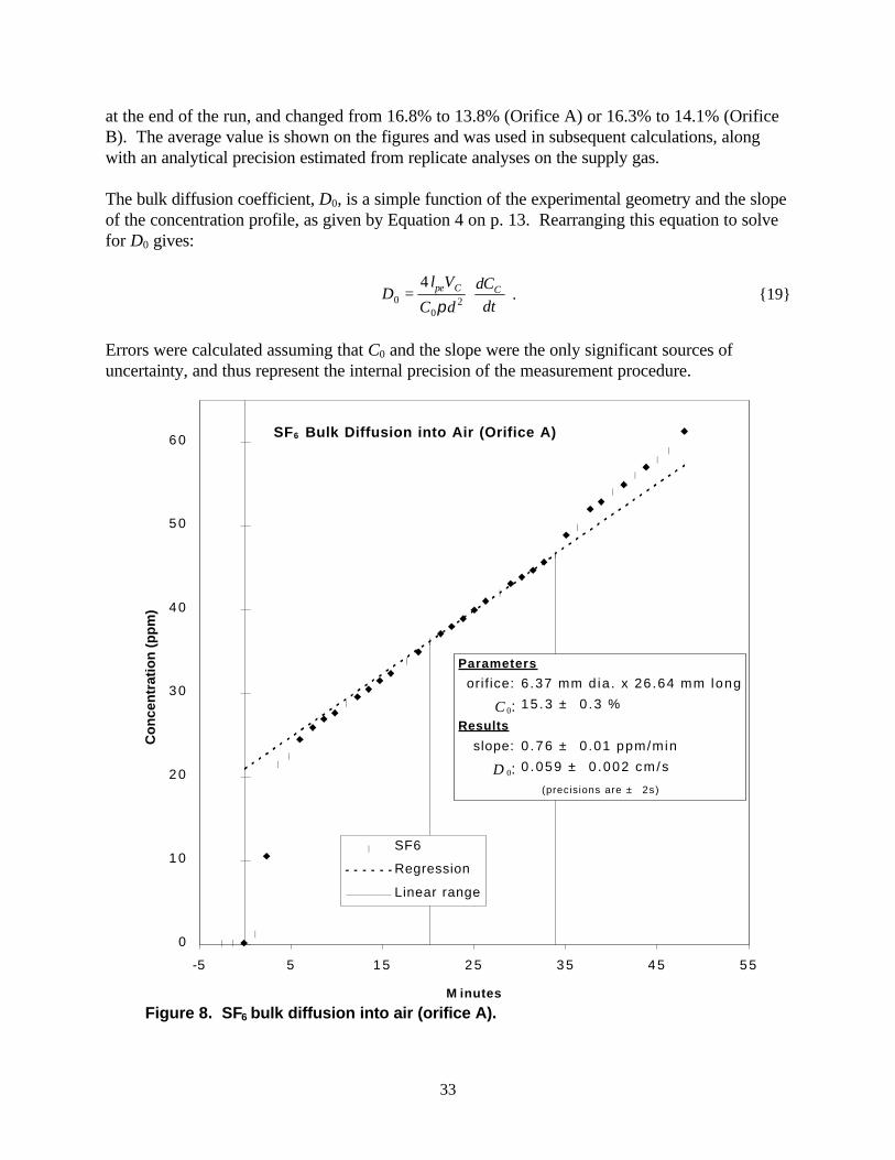
Collection-reservoir profiles for two different orifices are shown in Figures 8 and 9. Theconcentration jump between 0 and 5 minutes illustrates the effect of the slight pressure differentialpresent when SF6 was flowing into the supply reservoir. Slight irregularities in the trend of thedata at later times was probably due to fluctuations in ambient pressure in the laboratory as thebuilding ventilation system switched on and off. The supply reservoir was sampled at 5 min and

33

at the end of the run, and changed from 16.8% to 13.8% (Orifice A) or 16.3% to 14.1% (OrificeB). The average value is shown on the figures and was used in subsequent calculations, alongwith an analytical precision estimated from replicate analyses on the supply gas.

The bulk diffusion coefficient, D0, is a simple function of the experimental geometry and the slopeof the concentration profile, as given by Equation 4 on p. 13. Rearranging this equation to solvefor D0 gives:

Dl V

C ddCdt

pe C C0

02

4= ⋅

π . {19}

Errors were calculated assuming that C0 and the slope were the only significant sources ofuncertainty, and thus represent the internal precision of the measurement procedure.

0

1 0

2 0

3 0

4 0

5 0

6 0

-5 5 1 5 2 5 3 5 4 5 5 5

M inutes

Co

nce

ntr

atio

n (

pp

m)

SF6

Regression

Linear range

Parameters

orif ice: 6 .37 mm d ia . x 26.64 mm long

C0: 15 .3 ± 0 .3 %

Results

slope: 0 .76 ± 0 .01 ppm/min

D 0: 0 .059 ± 0 .002 cm/s

(precisions are ± 2s)

SF6 Bulk Diffusion into Air (Orifice A)

Figure 8. SF6 bulk diffusion into air (orifice A).

34

0

10

20

30

40

50

60

-5 5 15 25 35 45 55

M inutes

Co

nce

ntr

atio

n (

pp

m)

SF6

Regression

Linear range

Parameters

orif ice: 8.33 mm dia. x 26.72 mm long

C0: 15 .2 ± 0 .3 %

Results

slope: 1 .59 ± 0.02 ppm/min

D0: 0 .073 ± 0 .003 cm/s

(precis ions are ± 2s)

SF6 Bulk D iffusion into A ir (Orifice B)

Figure 9. SF6 bulk diffusion into air (orifice B).

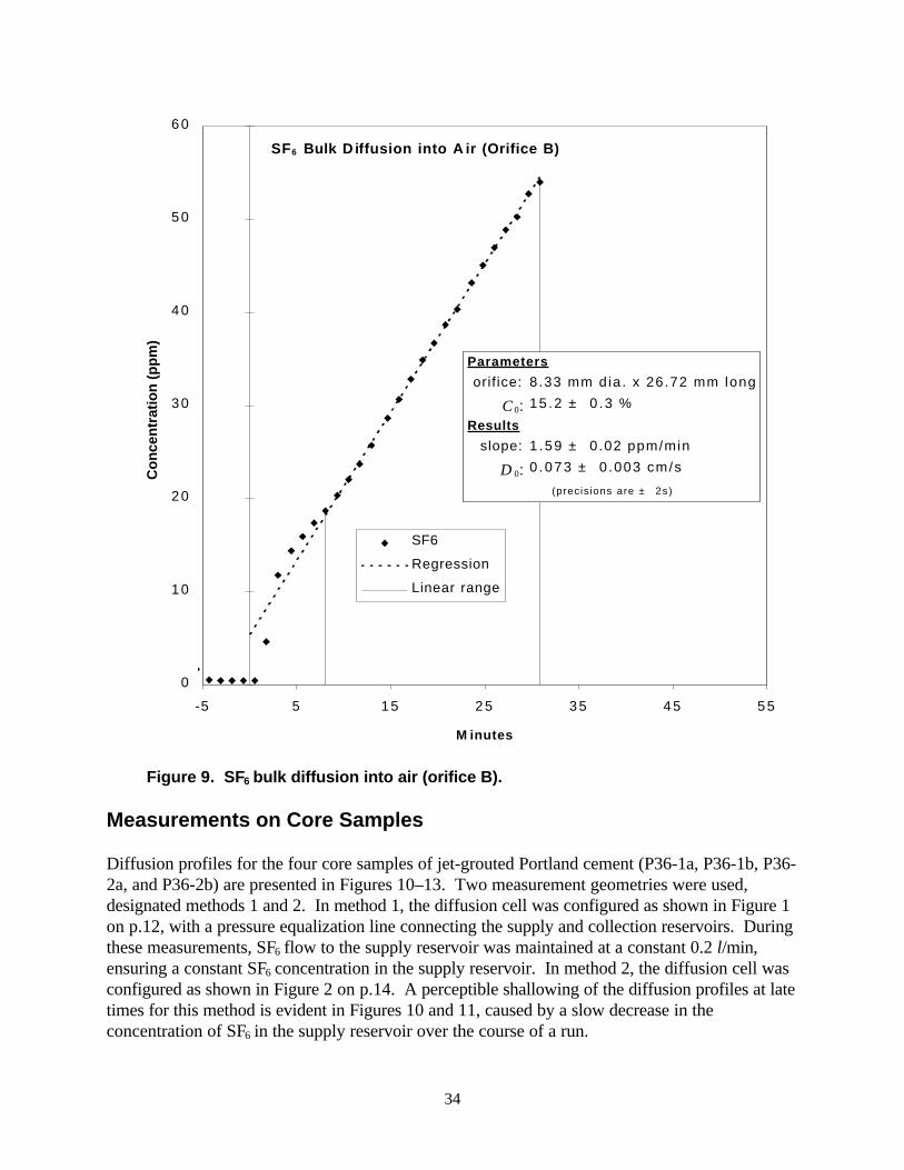
Measurements on Core Samples

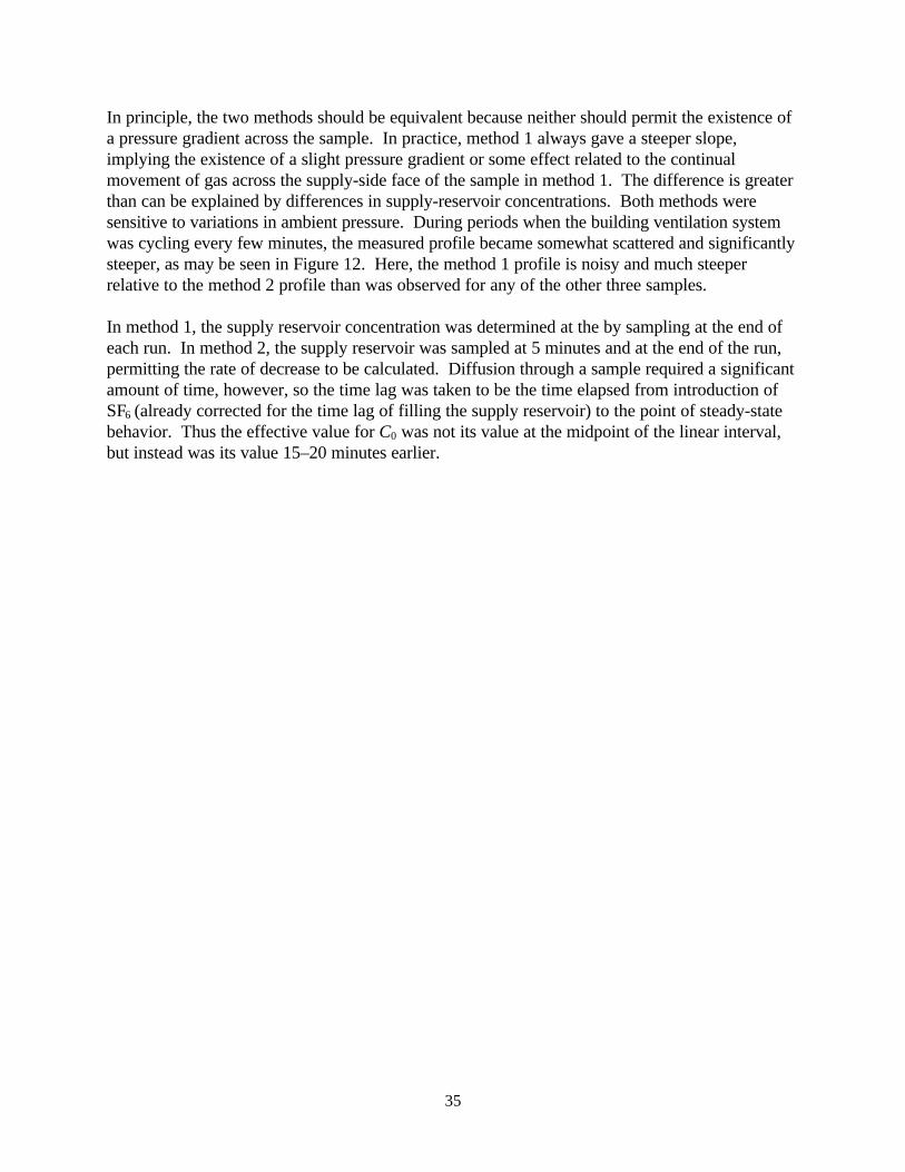
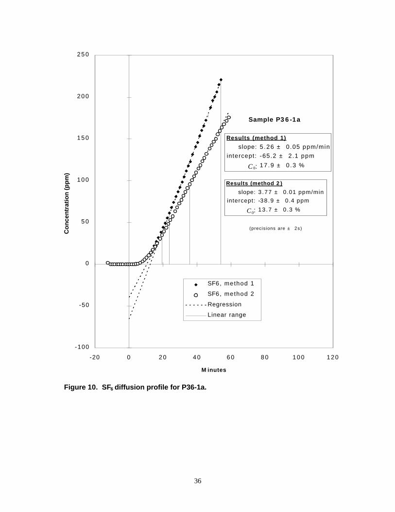
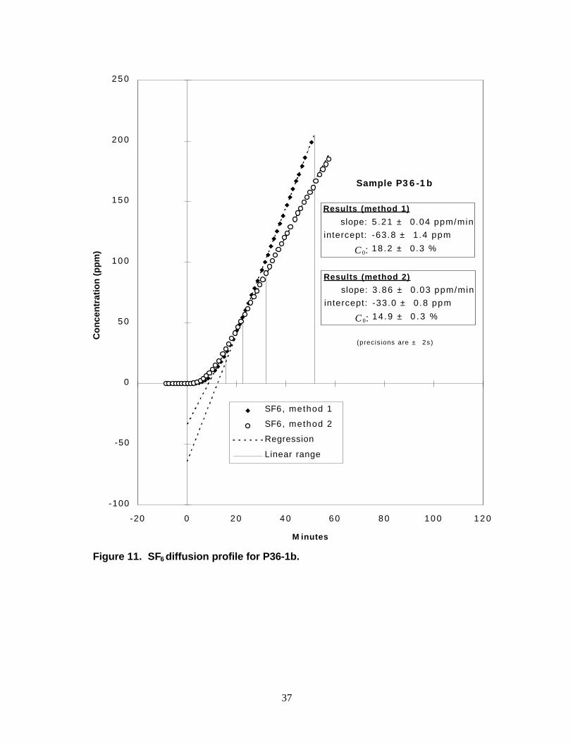
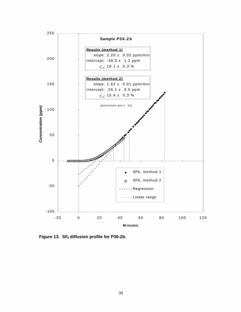
Diffusion profiles for the four core samples of jet-grouted Portland cement (P36-1a, P36-1b, P36-2a, and P36-2b) are presented in Figures 10–13. Two measurement geometries were used,designated methods 1 and 2. In method 1, the diffusion cell was configured as shown in Figure 1on p.12, with a pressure equalization line connecting the supply and collection reservoirs. Duringthese measurements, SF6 flow to the supply reservoir was maintained at a constant 0.2 l/min,ensuring a constant SF6 concentration in the supply reservoir. In method 2, the diffusion cell wasconfigured as shown in Figure 2 on p.14. A perceptible shallowing of the diffusion profiles at latetimes for this method is evident in Figures 10 and 11, caused by a slow decrease in theconcentration of SF6 in the supply reservoir over the course of a run.

35

In principle, the two methods should be equivalent because neither should permit the existence ofa pressure gradient across the sample. In practice, method 1 always gave a steeper slope,implying the existence of a slight pressure gradient or some effect related to the continualmovement of gas across the supply-side face of the sample in method 1. The difference is greaterthan can be explained by differences in supply-reservoir concentrations. Both methods weresensitive to variations in ambient pressure. During periods when the building ventilation systemwas cycling every few minutes, the measured profile became somewhat scattered and significantlysteeper, as may be seen in Figure 12. Here, the method 1 profile is noisy and much steeperrelative to the method 2 profile than was observed for any of the other three samples.

In method 1, the supply reservoir concentration was determined at the by sampling at the end ofeach run. In method 2, the supply reservoir was sampled at 5 minutes and at the end of the run,permitting the rate of decrease to be calculated. Diffusion through a sample required a significantamount of time, however, so the time lag was taken to be the time elapsed from introduction ofSF6 (already corrected for the time lag of filling the supply reservoir) to the point of steady-statebehavior. Thus the effective value for C0 was not its value at the midpoint of the linear interval,but instead was its value 15–20 minutes earlier.

36

-100

-50

0

50

100

150

200

250

-20 0 20 40 60 80 100 120

M inutes

Co

nce

ntr

atio

n (

pp

m)

SF6, method 1

SF6, method 2

Regression

Linear range

Sample P3 6 -1a

Results (method 1)

slope: 5 .26 ± 0.05 ppm/min

intercept: -65.2 ± 2.1 ppm

C0: 17 .9 ± 0 .3 %

Results (method 2 )

slope: 3 .77 ± 0.01 ppm/min

intercept: -38 .9 ± 0.4 ppm

C0: 13 .7 ± 0 .3 %

(precisions are ± 2s )

Figure 10. SF6 diffusion profile for P36-1a.

37

-100

-50

0

50

100

150

200

250

-20 0 20 40 60 80 100 120

M inutes

Co

nce

ntr

atio

n (

pp

m)

SF6, method 1

SF6, method 2

Regression

Linear range

Sample P3 6 -1 b

Results (method 1)

slope: 5 .21 ± 0.04 ppm/min

intercept: -63.8 ± 1.4 ppm

C0: 18.2 ± 0 .3 %

Results (method 2)

slope: 3 .86 ± 0.03 ppm/min

intercept: -33.0 ± 0 .8 ppm

C0: 14.9 ± 0 . 3 %

(precisions are ± 2s )

Figure 11. SF6 diffusion profile for P36-1b.

38

-100

-50

0

50

100

150

200

250

-20 0 20 40 60 80 100 120

M inutes

Co

nce

ntr

atio

n (

pp

m)

SF6, method 1

SF6, method 2

Regression

Linear range

Sample P3 6 -2a

Results (method 2)

slope: 1 .06 ± 0.01 ppm/min

intercept: -24.9 ± 0 .6 ppm

C0: 10.4 ± 0 . 3 %

Results (method 1)

slope: 2 .68 ± 0.05 ppm/min

intercept: -66.3 ± 4 .0 ppm

C0: 18.2 ± 0 . 3 %

(precisions are ± 2s )

Figure 12. SF6 diffusion profile for P36-2a.

39

-100

-50

0

50

100

150

200

250

-20 0 20 40 60 80 100 120

M inutes

Co

nce

ntr

atio

n (

pp

m)

SF6, method 1

SF6, method 2

Regression

Linear range

Sample P3 6 -2 b

Results (method 1)

slope: 2 .20 ± 0.02 ppm/min

intercept: -48.3 ± 1.2 ppm

C0: 18 .1 ± 0 .3 %

Results (method 2)

slope: 1 .62 ± 0.01 ppm/min

intercept: -26.1 ± 0.5 ppm

C0: 15 .4 ± 0 .3 %

(precisions are ± 2s )

Figure 13. SF6 diffusion profile for P36-2b.

40

Discussion

Bulk Diffusion Coefficient for SF6 Self-Diffusion

Before the expected time-dependent behavior of the diffusion measurements can be calculated, anestimate of the bulk diffusion rate of SF6 (D0) is needed. Stefanov et al. (1991) report a value forthe self-diffusion rate of SF6 calculated from their best-fit equation-of-state based on an exhaustivereview of the available experiments. Their value is ρD0 = 1.933 × 10–5 kg/m·s (interpolated) at25°C, where ρ is the density of the gas. Pure SF6 has a specific gravity of 5.13, and the density ofair at an ambient pressure of 626 torr is 0.976 kg/m3 at 25°C, so the density of pure SF6 would be5.01 kg/m3. Thus D0 should be 0.039 cm2/s.

The expected value of D0 can also be calculated from the kinetic theory of gases (cf. Atkins,1978):

D c013

= λ , where λσ

=1

2

kTp

and ckTm

=

81

2

π . {20}

Here, λ is the mean free path, c is the average molecular speed, σ is the effective molecularcollision cross-section (equal to πd2 where d is the molecular diameter), k is Boltzmann’sconstant, T is the absolute temperature, p is the pressure, and m is the molecular mass (146 g/molfor SF6). The molecular diameter of SF6 may be estimated from the radii of the constituent atomsand by assuming octahedral symmetry with the sulfur atom at the center. The molecular diameterwill be approximately the sum of the diameters of two fluorine atoms and one sulfur atom,corresponding to any corner-to-corner axis through the octahedron. Possible SF6 diameters aresummarized in Table 3 for various bonding assumptions. The temperature is assumed to be298.15 K (25.0 °C), and the pressure is taken to be 626 torr, reflecting the local air pressure inAlbuquerque, New Mexico at an elevation of ~1.8 km above sea level. Converting these valuesto internally consistent units for use in Equation 20 gives an average speed ( c ) of 208 m/s and amean free path (λ) of 290–558 Å, resulting in bulk diffusion coefficients (D0) of 0.022–0.039cm2/s.

The theoretical values are in good agreement with the experimentally derived value, despite thefact that the ratio of mean free path to molecular diameter is low (50–210). Both values apply tothe case of self-diffusion, however, rather than diffusion into air as is the case in the presentexperimental work. When SF6 is present at trace concentrations, collisions between SF6 moleculeswill be rare, so diffusion will be determined by the predominant heteromolecular collisionsbetween SF6 and N2 or O2. A preliminary literature search for information on the diffusion of SF6

into air was not fruitful, but based on the kinetic theory of gases, an argument for more rapiddiffusion can be made. In air, the massive SF6 molecules will collide more frequently with thelightweight N2 and O2 molecules than they would collide with other SF6 molecules in pure SF6, buttheir directions of travel will not be randomized as effectively because of their large inertia

41

compared to N2 and O2. The net result may be that the effective mean free path of SF6 in air isgreater than in pure SF6, and hence diffusion in air would be more rapid also.

Table 3. Theoretical diffusion rates for SF6.

Bonding Sulfur dia. (Å) Fluorine dia. (Å) SF6 dia. (Å) D0 (cm2/s)

ionic 0.60 2.66 5.92 0.022covalent 2.04 1.44 4.92 0.032atomic 2.18 1.14 4.46 0.039

Measured Bulk Diffusion for SF6 Diffusion into Air

The bulk diffusion coefficient for SF6 into air was measured using orifices of two differentdiameters. The larger orifice gave the highest value, of 0.073 cm/s, whereas the smaller orificegave a value of 0.059 cm/s. Both values are larger than either the measured self-diffusioncoefficient or the theoretical values derived from the kinetic theory of gases, described above.Undoubtedly part of the discrepancy is due to a mixing effect on the collection-reservoir side ofthe orifice related to the motion of the air as it was stirred by the fan. Mixing would tend toshorten the effective length of the orifice, causing the calculated value of D0 to be too high. Itwould also have a greater effect on the larger diameter orifice because mixing could penetratefarther into the orifice due to the larger opening. Additional uncertainty is introduced by theunknown effects of variations in ambient pressure.

The present data only loosely constrain the value of D0 for air, but suggest that it may be largerthan the self-diffusion D0 value. The larger of the two measured values (0.073 cm/s) is likely tobe an upper limit, and will be used as a limiting case in the remainder of this discussion. The valueof 0.039 cm/s from the self-diffusion discussion will be taken as the likely lower limit.

Expected Time-Dependent Diffusion in Portland Cement

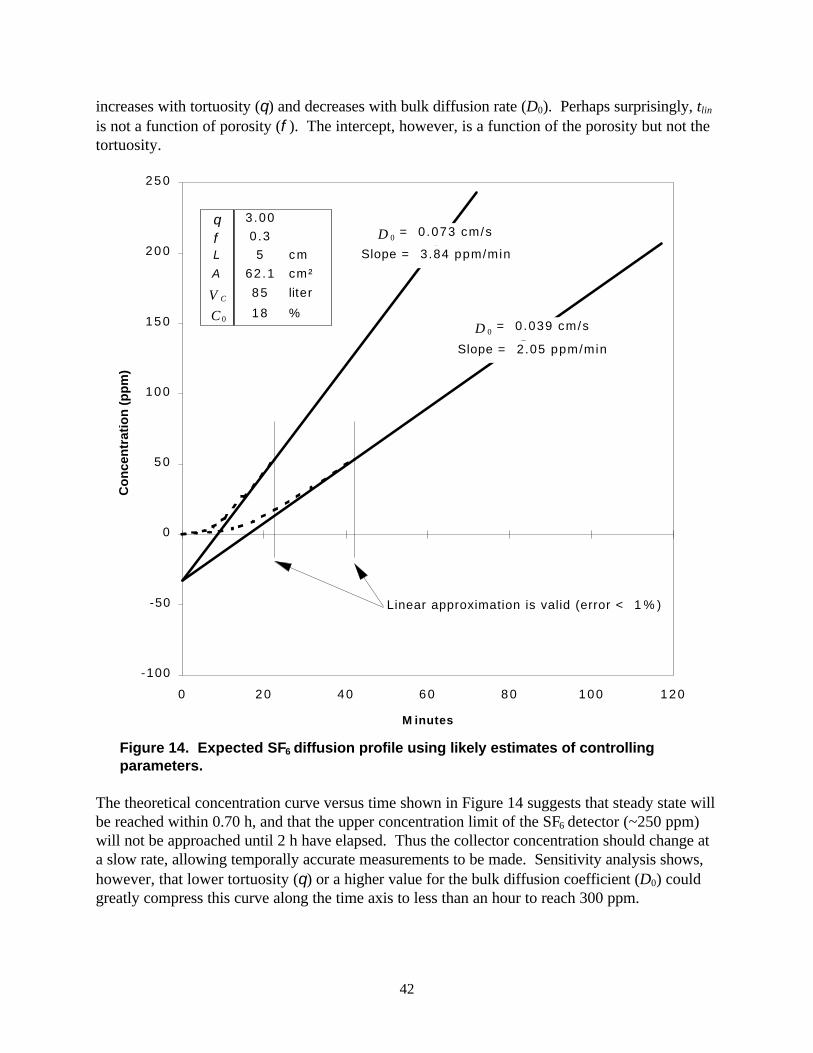
The expected time-dependent behavior of the diffusion measurements can now be calculated giventhe geometry of the diffusion cell and estimated sample parameters. Results are shown in Figure14 for a set of parameters that may resemble porous Portland cement. The porosity, φ, was set to0.30, a value typical of fine-grained materials. The tortuosity, θ, was taken to be 3.00, to giveprofiles similar to those measured experimentally. This may be unrealistically low if this term is tobe interpreted geometrically, however; Dykhuizen and Casey (1989) obtained a value for dolomiteof 4.36. For a diffusion rate in air, D0, of 0.039 cm2/s. This calculation predicts that steady-stateshould be reached in ~1.5 h, and that after 4 h the concentration of SF6 in the collection reservoir(CC) will still be less than ~250 ppm, corresponding to a rate of increase of 1.08 ppm/min. Asmay be seen from Equation 8 on p. 15, the rate of increase is directly proportional to the samplediffusion coefficient (DS), which in turn is directly proportional to the bulk diffusion coefficient(D0) and the porosity (φ), and inversely proportional to the square of the tortuosity (θ) (Equation9 on p. 15). Less obvious is the relation between these parameters and the time required to reachsteady-state (tlin), defined here as the time at which the linear approximation differs from the exactsolution by less than 1%. Sensitivity analysis confirms the intuitive relations, showing that tlin

42

increases with tortuosity (θ) and decreases with bulk diffusion rate (D0). Perhaps surprisingly, tlin

is not a function of porosity (φ). The intercept, however, is a function of the porosity but not thetortuosity.

-100

-50

0

50

100

150

200

250

0 20 40 60 80 100 120

M inutes

Co

nce

ntr

atio

n (

pp

m)

θ 3.00

φ 0.3

L 5 cm

A 62.1 cm²

V C 85 liter

C0 18 %

Linear approximation is valid (error < 1 % )

Slope = 3.84 ppm/min

D0 = 0 .073 cm/s

Slope = 2.05 ppm/min

D0 = 0 .039 cm/s

Figure 14. Expected SF6 diffusion profile using likely estimates of controllingparameters.

The theoretical concentration curve versus time shown in Figure 14 suggests that steady state willbe reached within 0.70 h, and that the upper concentration limit of the SF6 detector (~250 ppm)will not be approached until 2 h have elapsed. Thus the collector concentration should change ata slow rate, allowing temporally accurate measurements to be made. Sensitivity analysis shows,however, that lower tortuosity (θ) or a higher value for the bulk diffusion coefficient (D0) couldgreatly compress this curve along the time axis to less than an hour to reach 300 ppm.

43

A factor that was not considered in the theoretical treatment is that SF6 is diffusing from a regionwhere it is present at 20% (with the balance made up of N2) to a region containing air (21% O2,78% N2, 1% Ar) where it is essentially absent. A concentration gradient similar to that drivingSF6 diffusion, but in the opposite direction, will drive diffusion of O2 from the collection reservoirtoward the SF6 supply reservoir. The rate of diffusion of O2 will be higher than for SF6, perhapsby a factor of five, because of its smaller size and lower mass. Although transport of O2 into thesupply reservoir will exceed diffusion of SF6 out of it, no pressure gradient will develop becauseboth the supply and collection reservoirs are vented to the atmosphere. The O2 diffusion mightsignificantly dilute the supply gas, depending upon sample properties. If enough SF6 diffusesthrough to raise its concentration in the 75-liter collection reservoir to 300 ppm, ~5 times as muchO2 may diffuse into the supply reservoir. If the supply reservoir has volume of 0.25 liters, thiswould correspond to a volume fraction of the supply reservoir of : 300 ppm SF6 × 75 liters ×DO2/DSF6(= ~5) × 1/0.25 liters = 45%. Clearly, however, the O2 concentration in the SF6 reservoircannot exceed that in air (21%), and more likely will be only half as much (10%) or less. Tocorrect for this, the SF6 concentration in the supply reservoir was monitored at the end of each runto assess the extent of dilution.

Experimental Measurements and Derived Parameters

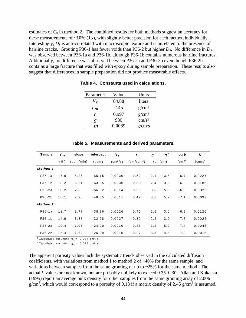
The raw experimental data of slope and intercept provides the necessary inputs for calculatingtransport parameters, as listed in Table 5. Constants used in the calculations are given in Table 4.The effective diffusion coefficient (DS) for each sample was calculated using Equation 8 (p.15). Itdepends only on the slope, the supply reservoir concentration (C0) and the physical dimensions ofthe sample and diffusion cell; it is the proportionality constant relating flux to concentrationgradient. The porosity (φ) is similarly fundamental, depending only on the intercept and on C0

and the physical dimensions. It was calculated using Equation 12 on p.16. At a greater level ofabstraction is the tortuosity (θ, the ratio of the actual average path length to the sample length),which is derived from DS, φ, and the bulk diffusion coefficient (D0) according to Equation 9 onp.15.

The diffusive properties are related to fluid flows due to differences in piezometric head by theKozeny-Carman equation (Equation 16 on p.17) for permeability (k) and the general equation forhydraulic conductivity (K, Equation 14 on p.17). The Kozeny-Carman equation provides anempirical relation between φ and k, and also requires an estimate of the specific surface area andthe density of the matrix. The matrix density of Portland cement was taken to be the average ofportlandite (ρ = 2.24 g/cm3) and quartz (a representative soil mineral, with ρ = 2.65 g/cm3),giving a value of 2.45 g/cm3 for ρm. Equation 14 on p.17 relates K to k and the fluid’s density

and dynamic viscosity, given in Table 4 for pure water at 25°C.

The effective diffusion coefficients appear to be significantly different between the two groutingsthat were sampled. Both experimental methods gave similar results for DS, averaging 0.0028 forP36-1 and 0.0011 for P36-2, values over an order of magnitude less than for SF6 diffusion in air(D0). Method 1, with continuous SF6 flow, yielded slightly higher DS values for all four samples,due either to the presence of a slight pressure differential in this method, or to inaccurate

44

estimates of C0 in method 2. The combined results for both methods suggest an accuracy forthese measurements of ~10% (1σ), with slightly better precision for each method individually.Interestingly, DS is anti-correlated with macroscopic texture and is unrelated to the presence ofhairline cracks. Grouting P36-1 has fewer voids than P36-2 but higher DS. No difference in DS

was observed between P36-1a and P36-1b, although P36-1b contains numerous hairline fractures.Additionally, no difference was observed between P36-2a and P36-2b even though P36-2bcontains a large fracture that was filled with epoxy during sample preparation. These results alsosuggest that differences in sample preparation did not produce measurable effects.

Table 4. Constants used in calculations.

Parameter Value UnitsVc 84.88 litersρm 2.45 g/cm³

ρ 0.997 g/cm³g 980 cm/s²µ 0.0089 g/cm·s

Table 5. Measurements and derived parameters.

Sample CC 00 slope intercept DD SS φφ θ θ 1 θ θ 2 log kk KK

(% ) (ppm/min) (ppm) (cm²/s) (cm³ /cm³) (cm/cm) (cm²) (cm/s)

M ethod 1

P36-1a 1 7 . 9 5 . 2 6 - 6 5 . 1 5 0 . 0 0 3 0 0 . 5 2 2 . 4 3 . 5 -6 .7 0 . 0 2 2 7

P36 -1b 1 8 . 2 5 . 2 1 - 6 3 . 8 5 0 . 0 0 3 0 0 . 5 0 2 . 4 3 . 5 -6 .8 0 . 0 1 8 6

P36-2a 1 8 . 2 2 . 6 8 - 6 6 . 3 2 0 . 0 0 1 4 0 . 5 5 3 . 6 5 . 3 -6 .5 0 . 0 3 2 5

P36 -2b 1 8 . 1 2 . 2 0 - 4 8 . 3 5 0 . 0 0 1 1 0 . 4 2 3 . 6 5 . 2 -7 .1 0 . 0 0 9 7

M ethod 2

P36-1a 1 3 . 7 3 . 7 7 - 3 8 . 8 6 0 . 0 0 2 6 0 . 4 5 2 . 6 3 . 6 -6 .9 0 . 0 1 2 6

P36 -1b 1 4 . 9 3 . 8 6 - 3 2 . 9 8 0 . 0 0 2 7 0 . 3 2 2 . 2 3 . 0 -7 .7 0 . 0 0 2 2

P36-2a 1 0 . 4 1 . 0 6 - 2 4 . 9 0 0 . 0 0 1 0 0 . 3 6 3 . 8 5 . 2 -7 .4 0 . 0 0 4 5

P36 -2b 1 5 . 4 1 . 6 2 - 2 6 . 0 9 0 . 0 0 1 0 0 . 2 7 3 . 3 4 . 5 -7 .9 0 . 0 0 1 51

Calculated assuming D 0 = 0 .034 cm² / s .2

Calculated assuming D 0 = 0 .073 cm² / s .

The apparent porosity values lack the systematic trends observed in the calculated diffusioncoefficients, with variations from method 1 to method 2 of ~40% for the same sample, andvariations between samples from the same grouting of up to ~25% for the same method. Theactual φ values are not known, but are probably unlikely to exceed 0.25–0.30. Allan and Kukacka(1995) report an average bulk density for other samples from the same grouting array of 2.006g/cm3, which would correspond to a porosity of 0.18 if a matrix density of 2.45 g/cm3 is assumed.

45

Several factors may have contributed to these scattered and seemingly large porosity values, suchas an inaccurate estimate of the time required to fill the supply reservoir before diffusion can besaid to begin, variation of D0 as a function of its concentration in air, and decreases in the ambientpressure causing unaccounted-for delays in the attainment of steady-state. All of these factorscould affect the value of the intercept at t = 0. For lack of better estimates of φ, however, thesevalues will be used in the subsequent analysis for θ, k, and K.

Surprisingly, the tortuosity shows greater consistency than the porosity, in part because it isrelated to the square root of the porosity (and D0, and 1/DS). Tortuosities were calculated forlimiting values of D0 (0.034 and 0.073 cm/s). Use of the higher value led to θ values of 3.0–5.3,bracketing the value observed by Dykhuisen and Casey (1989) of 4.36. The following discussionuses the higher D0 value. Both method 1 and method 2 indicate that grouting P36-1 has a lowertortuosity (~3.4) than P36-2 (~4.9). Further work is needed to determine the extent to whichthese tortuosities have physical significance. It is suggestive, however, that the grouting with lowDS has high θ.

Calculated permeabilities are near 10-7 cm2, giving rise to calculated conductivities near 10-2 cm/sfor all four samples. Method 1 gave somewhat greater values due to the greater porositiesdiscussed previously. These conductivities are much higher than those reported by Allan andKukacka (1995) for other samples from the same grouting array, which were in the range10-8–10-9 cm/s. Allan and Kukacka made their measurements under saturated aqueous conditions,however, where the cement gel in these groutings would have swelled significantly (Lea, 1971).This would have reduced porosity and drastically constricted the throats between adjoining pores,thereby greatly reducing permeability and hydraulic conductivity. Thus, gas permeability isexpected to be much greater than aqueous permeability for cement-based materials, but this maynot be responsible for the entire six-order-of-magnitude difference. Recall that the Kozeny-Carman equation, used to related porosity and specific surface area to conductivity, wascalibrated empirically for granular media, so some degree of inaccuracy is to be expected whenapplying it to a porous gel such as cement. Resolution of this issue will require furtherintercomparisons of gas-diffusion versus saturated aqueous methods, including measurements onsamples of stable geometry (i.e., non-swelling in the presence of water).

Feasibility of Field-Scale Measurements

Gas diffusion measurements show promise as a tool for studying the integrity on barriers in fieldsettings, in addition to evaluating ex situ prepared samples in the laboratory. Diffusion of SF6

through grout (a mixture of soil and cement) is at least an order of magnitude slower thandiffusion through air, so the method should be sensitive to the presence of open fractures, largevoids, or other discontinuities in the grout. Nevertheless, diffusion of SF6 through grout is rapidenough so that measurements will require a matter of days rather than months or years. The timerequired to reach steady state is proportional to the square of the length over which diffusion is tobe measured (cf. Equation 11 on p.16), so extrapolating from the laboratory where ~20 min wasrequired to reach steady-state for a 5 cm length to a distance of 1 m in the field suggests that ~5.6days would be required. The principle difficulty may be to minimize alternate flow paths betweensource and detector, either through the soil or the ambient atmosphere rather than the barrier.

46

Gas diffusion presents an important advantage relative to aqueous tracer studies under fieldconditions to verify the integrity of a barrier: it is essentially non-destructive. In oneconceptualization, a small hole could be bored to the center of the barrier for the introduction ofSF6, and an array of sniffers could be located around the outside of the barrier. (The snifferswould be multiplexed to a single gas analyzer and would be sampled sequentially.) Gas could beintroduced at atmospheric pressure to ensure only diffusional transport, or at slightly elevatedpressure to speed up the approach to steady state and increase the flux to the sniffers. Integritywould be assessed by comparing observed profiles of concentration versus time with predictionsbased on the barrier geometry. Empirical assessment might also be possible by taking advantageof any symmetry in the barrier geometry and comparing equivalent flow paths.

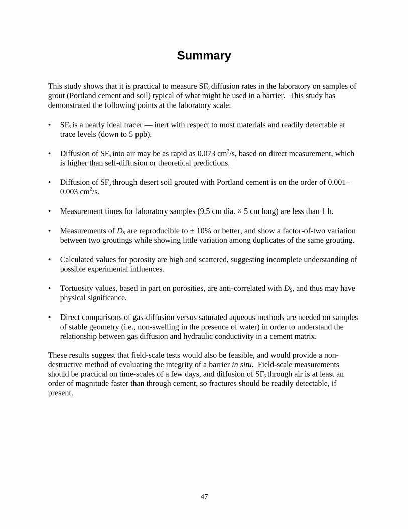
47

Summary

This study shows that it is practical to measure SF6 diffusion rates in the laboratory on samples ofgrout (Portland cement and soil) typical of what might be used in a barrier. This study hasdemonstrated the following points at the laboratory scale:

• SF6 is a nearly ideal tracer — inert with respect to most materials and readily detectable attrace levels (down to 5 ppb).

• Diffusion of SF6 into air may be as rapid as 0.073 cm2/s, based on direct measurement, whichis higher than self-diffusion or theoretical predictions.

• Diffusion of SF6 through desert soil grouted with Portland cement is on the order of 0.001–0.003 cm2/s.

• Measurement times for laboratory samples (9.5 cm dia. × 5 cm long) are less than 1 h.

• Measurements of DS are reproducible to ± 10% or better, and show a factor-of-two variationbetween two groutings while showing little variation among duplicates of the same grouting.

• Calculated values for porosity are high and scattered, suggesting incomplete understanding ofpossible experimental influences.

• Tortuosity values, based in part on porosities, are anti-correlated with DS, and thus may havephysical significance.

• Direct comparisons of gas-diffusion versus saturated aqueous methods are needed on samplesof stable geometry (i.e., non-swelling in the presence of water) in order to understand therelationship between gas diffusion and hydraulic conductivity in a cement matrix.

These results suggest that field-scale tests would also be feasible, and would provide a non-destructive method of evaluating the integrity of a barrier in situ. Field-scale measurementsshould be practical on time-scales of a few days, and diffusion of SF6 through air is at least anorder of magnitude faster than through cement, so fractures should be readily detectable, ifpresent.

48

Intentionally Left Blank

49

References

Allan, M.L. and L.E. Kukacka, 1994: In-Situ Containment and Stabilization of Buried Waste.Fiscal year 1994 Annual Report BNL-60977, Brookhaven National Laboratory, Upton, NewYork.

Allan, M.L. and L.E. Kukacka, 1995: Analysis of CoreSamples from Jet Grouted Soil. Informal Report BNL-62357, Brookhaven NationalLaboratory, Upton, New York, 13 p.

Atkins, P.W., 1978: Physical Chemistry. W.H. Freeman and Co., San Francisco, California,1018 p.

Bear, J., 1972: Dynamics of Fluids in Porous Media. Dover Publications, Inc., New York,764 p.

Carslaw, H.S. and J.C. Jaeger, 1959: Conduction of Heat in Solids, Second Edition. OxfordUniversity Press, New York, 510 p.

Dykhuizen, R.C. and W.H. Casey, 1989: An Analysis of Solute Diffusion in Rocks. Geochimicaet Cosmochimica Acta, v. 53, p. 2797–2805.

Franz, E.-M., M. Fuhrmann, B. Bowerman, S. Bates, and R. Peters, 1994: Proposed Waste FormPerformance Criteria and Testing Methods for Low-Level Mixed Waste. BrookhavenNational Laboratory Formal Report, BNL-52436 or DOE/MWIP-30, 153 p.

Heiser, J. and B. Dwyer, 1995: Demonstration of Close-Coupled Barriers for SubsurfaceContainment of Buried Waste. Informal Report BNL-62573, Brookhaven NationalLaboratory, Upton, New York, 65 p.

Lea, F.M., 1971: The Chemistry of Cement and Concrete. Chemical Publishing Co., New York,727 p.

Stefanov, B., L. Zarkova, L.R. Folkin, V.E. Lyusternik, V.V. Altunin, and E.E. Tozkii, 1991:Thermophysical Properties of Gaseous Sulphur Hexafluoride in the Range 220–1000 K: 43Experiments Described by a Unique Intermolecular Potential. High Temperatures-HighPressures, v. 23, p. 461–471.

Weast, R.C., 1973: Handbook of Chemistry and Physics. CRC Press, Inc., Cleveland, OH.

50

Distribution

3 U.S. Department of EnergyAttn: Skip ChamberlainEM-54, Cloverleaf Center19901 Germantown Rd.Germantown, MD 20874-12901

1 U.S. Department of EnergyAttn: Caroline PurdyEM-53, Cloverleaf Center19901 Germantown Rd.Germantown, MD 20874-12901

1 U. S. Department of EnergySavannah River Operations OfficeAttn: Scott McMullinBuilding 703-46AP.O. Box AAiken, SC 29802

1 U. S. Department of EnergySavannah River Operations OfficeEnvironmental Sciences SectionAttn: Mike SerratoP.O. Box 616 / 773-42AAiken, SC 29802

1 U. S. Department of EnergyAlbuquerque Operations Office, ETNAttn: Dennis OlonaPennsylvania/H StreetAlbuquerque, NM 87116

1 Brookhanven National LaboratoyAttn: John Heiser34 North Railroad Ave.Building 830Upton, NY 11973

1 Science & Engineering Associates, Inc.Attn: Sandy Dalvit Dunn1570 Pacheco, Suite D-1Santa Fe, NM 87501

1 Thomas Branigan LibraryAttn: D. Dresp106 W. Hadley St.Las Cruces, NM 88003

1 Government Publications DepartmentZimmerman LibraryUniversity of New MexicoAlbuquerque, NM 87131

3 MS0706 C.V. Williams, 61131 0719 G. C. Allen, 66211 0719 J. D. Betsill, 66215 0719 T. D. Burford, 66211 9018 Central Technical Files, 8940-25 0899 Technical Library, 49162 0619 Review & Approval Desk, 12690

for DOE/OSTI