GPCP V2.2 1

GPCP Version 2.2 Combined Precipitation Data Set Documentation

George J. Huffman David T. Bolvin

Laboratory for Atmospheres, NASA Goddard Space Flight Center

and Science Systems and Applications, Inc.

July 27, 2011

What’s New! July 29, 2011 Version 2.2 of the monthly Satellite-Gauge (SG) combined precipitation data set has been released, superseding all previous versions, including Version 2.1. This upgrade takes advantage of upgrades in many of the constituent datasets, including the Chang/Chiu/Wilheit (CCW) emission and NOAA scattering algorithms, the GPCC precipitation gauge analysis, and inclusion of the DMSP F17 SSMIS.

July 6, 2009 Version 2.1 has been released, superseding all previous versions, including Version 2. This change was driven by changes to the GPCC gauge analysis, and includes rescaling the OPI estimates that are used in the pre-SSMI era. Version 2.1 land estimates are generally higher than for Version 2, and the pre-SSMI ocean estimates are also higher. However, the OPI estimates in the pre-SSMI era still underestimate the variance that the SSMI-era estimates display. April 9, 2008 The October, November, and December 2007 GPCP data sets have been re-computed and re-posted. This action became necessary when processing problems in the AIRS data required a reprocessing for that data set by the AIRS data center; AIRS data are used in the GPCP products, predominantly at high latitudes. Users are urged to re-acquire these months of data and discard the previous version. February 25, 2008 The IDL procedure file read_v2_file.pro is now available to read the header and entire set of months in a Version 2.1 file into an IDL structure. June 20, 2006 The multi-satellite precipitation product has been recomputed for the span 1987 - 2006 to eliminate the inhomogeneity across the 1986/1987 (OPI/SSMI) data boundary over land. These data are now suitable for long-term studies using the entire data record. These files have

At present the months that use F17 SSMIS data (January 2009 to the delayed present), the NOAA PR2 algorithm during the outage of the 85 GHz channels on F08 (June 1990 through December 1991), and the partially sampled months of F08 (July 1987, January 1998, and December 1991) are being released in “provisional” status until final adjustments are developed, at which point revised datasets will supersede the provisionals.

GPCP V2.2 2

the format gpcp_v2_pms.YYYY, where YYYY is the 4-digit year. This documentation will be updated shortly to reflect this change to the multi-satellite precipitation product. June 14, 2006 The GPCP V2 estimates have been recomputed for the span May 2005 - February 2006 due to the recomputation of input AIRS estimates. The AIRS definition of "day" was inconsistent with the GPCP definition, so the AIRS estimates were recomputed to match the GPCP. The impact is minimal on the monthly V2 estimates. April 24, 2006 Beginning with May 2005, AIRS precipitation estimates have replaced the TOVS estimates at high latitudes because of TOVS instrument termination. The new AIRS data has been adjusted to match the large-scale bias of the TOVS to maintain homogeneity across the data boundary. For simplicity, any distributed dataset that depends on TOVS before May 2005 will utilize AIRS data in place of the TOVS as of that date. This applies to the datasets ending in "pst", "est", "ptv", "pms", "ems", "psg", and "esg".

Request to Users The GPCP datasets are developed and maintained with international cooperation and are used by the worldwide scientific community. To better understand the evolving requirements across the GPCP user community and to increase the utility of the GPCP product suite, the dataset producers request that a citation be provided for each publication that uses the GPCP products. Please email the citation to george.j.huffman@nasa.gov or david.t.bolvin@nasa.gov. Your help and cooperation will provide valuable information for making future enhancements to the GPCP product suite.

Contents

1. Data Set Names and General Content 2. Related Projects, Data Networks, and Data Sets 3. Storage and Distribution Media 4. Reading the Data 5. Definitions and Defining Algorithms 6. Temporal and Spatial Coverage and Resolution 7. Production and Updates 8. Sensors 9. Error Detection and Correction 10. Missing Value Estimation and Codes 11. Quality and Confidence Estimates 12. Data Archives 13. Documentation 14. Inventories 15. How to Order and Obtain Information about the Data

GPCP V2.2 3

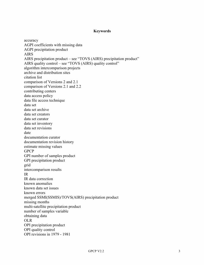
Keywords

accuracy AGPI coefficients with missing data AGPI precipitation product AIRS AIRS precipitation product – see “TOVS (AIRS) precipitation product” AIRS quality control – see “TOVS (AIRS) quality control” algorithm intercomparison projects archive and distribution sites citation list comparison of Versions 2 and 2.1 comparison of Versions 2.1 and 2.2 contributing centers data access policy data file access technique data set data set archive data set creators data set curator data set inventory data set revisions date documentation curator documentation revision history estimate missing values GPCP GPI number of samples product GPI precipitation product grid intercomparison results IR IR data correction known anomalies known data set issues known errors merged SSMI(SSMIS)/TOVS(AIRS) precipitation product missing months multi-satellite precipitation product number of samples variable obtaining data OLR OPI precipitation product OPI quality control OPI revisions in 1979 - 1981

GPCP V2.2 4

OPI revision to October 1985 originating machine pentads period of record precipitation variable production and updates products provisional data set quality index rain gauge rain gauge number of samples product rain gauge precipitation product rain gauge quality control random error read a month of a product read a month of byte-swapped product read the header record read the monthly climatology references satellite-gauge precipitation product similar data sets source variable spatial coverage spatial resolution SSMI (SSMIS) SSMI (SSMIS) composite number of samples product SSMI (SSMIS) composite precipitation product SSMI (SSMIS) emission number of samples product SSMI (SSMIS) emission precipitation product SSMI (SSMIS) error detection/correction SSMI (SSMIS) scattering number of samples product SSMI (SSMIS) scattering precipitation product standard missing value technique temporal resolution TOVS TOVS (AIRS) precipitation product TOVS (AIRS) quality control units of the variables variable

Acronyms 1DD One Degree Daily AGPI Adjusted GPI ASCII American Standard Code for Information Interchange (i.e., text)

GPCP V2.2 5

AIP Algorithm Intercomparison Project AIRS Atmospheric Infrared Sounder AVHRR Advanced Very High Resolution Radiometer CPC Climate Prediction Center CGMS Coordinating Group for Meteorological Satellites CLIMAT Climatological data (GTS coding) CMAP CPC Merged Analysis of Precipitation CPU Central Processing Unit (of a computer) DMSP Defense Meteorological Satellite Program DWD Deutscher Wetterdienst (German Weather Service) ENSO El Niño-Southern Oscillation FNMOC Fleet Numerical Meteorological and Oceanographic Center FTP File Transfer Protocol GARP Global Atmospheric Research Programme GATE GARP Atlantic Tropical Experiment Geo Geosynchronous GEWEX Global Energy and Water Cycle Experiment GHCN Global Historical Climate Network GMDC GPCP Merge Development Centre GMS Geosynchronous Meteorological Satellite GOES Geosynchronous Operational Environmental Satellites GPCC Global Precipitation Climatology Centre GPCP Global Precipitation Climatology Project GPI GOES Precipitation Index GSFC Goddard Space Flight Center GSPDC Geostationary Satellite Precipitation Data Centre GTS Global Telecommunications System HIRS2 High-Resolution Infrared Sounder 2 IDL Interactive Data Language IEEE Institute of Electrical and Electronics Engineers IPWG International Precipitation Working Group IR Infrared lat/lon latitude/longitude Leo Low-Earth-orbit MB megabytes Meteosat Meteorological Satellite MSU Microwave Sounding Unit MTSAT Ministry of Transportation Satellite NASA National Aeronautics and Space Administration NCDC National Climatic Data Center NCEP National Centers for Environmental Prediction NESDIS National Environmental Satellite Data and Information Service NOAA National Oceanic and Atmospheric Administration OLR Outgoing Longwave Radiation OPI OLR Precipitation Index PEHRPP Project for the Evaluation of High-Resolution Precipitation Products

GPCP V2.2 6

PIP Precipitation Intercomparison Project RSS Remote Sensing Systems SRDC Surface Reference Data Center SSMI Special Sensor Microwave/Imager SSMIS Special Sensor Microwave Imager-Sounder SSM/T2 Special Sensor Microwave/Temperature 2 Ta Antenna Temperature Tb Brightness Temperature TIROS Television Infrared Operational Satellite TOVS TIROS Operational Vertical Sounder UTC Universal Coordinated Time (same as GMT, Z) WCRP World Climate Research Programme WMO World Meteorological Organization 1. Data Set Names and General Content The *data set* is formally referred to as the "GPCP Version 2.2 Combined Precipitation Data Set". It is also referred to as the "Version 2.2 Data Set." The Version 2.2 data set supersedes the previous Version 1, 1c, V2X79, 2, and 2.1 data sets, which are now considered obsolete. The current data set provides two final products, the combined satellite-gauge (SG) precipitation estimate and the combined satellite-gauge precipitation error estimate. The complete data set, which includes the input and intermediate data files, contains a suite of 27 products providing monthly, global gridded values of precipitation totals and supporting information for the period January 1979 – (delayed) present. Since no single satellite data source spans the entire data record, the product draws upon many different sources covering different times within the entire data record. The periods of differing data coverage are January 1979 – December 1985, January 1986 – June 1987 (and December 1987), July 1987 – April 2005 (excluding December 1987), May 2005 – December 2008, and January 2009 – present. The data contributing to the resulting precipitation estimates for each of these four periods is discussed in section 5. Substantial attempts have been made to ensure consistency among the different available input sources. The main refereed citation for the data set is Adler et al. (2003; all references are listed in section 13), with the shift from Version 2 to Version 2.1 described in Huffman et al. (2009). The earlier Version 1 is documented in Huffman et al. (1997), which also appears in Huffman (1997b). ........................................................................... The GPCP Version 2.2 Data Set is currently considered a *provisional data set* because the GMDC has made temporary adjustments to the input datasets at several points to enable release of the entire dataset while the input dataset issues are resolved. This includes the months of GPCP Version 2.2 data involving F17 (January 2009 – present), NOAA F08 SSMI PR2 estimates (June 1990 – December 1991), and partially sampled months of F08 (July 1987, January 1988, and December 1991). The “provisional” label indicates that the developers believe the data for these months to be useful, but that users should exercise caution in cross-

GPCP V2.2 7

checking unexpected features. This is particularly the case for coasts, near-coastal ocean regions, islands, and small peninsulas, which are less likely to have the gauge coverage necessary to control possible biases in the provisional estimates. ........................................................................... 2. Related Projects, Data Networks, and Data Sets The *data set creators* are G.J. Huffman, D.T. Bolvin, and R.F. Adler, working in the Laboratory for Atmospheres, NASA Goddard Space Flight Center, Code 613.1, Greenbelt Maryland, USA, as the GPCP Merge Development Centre. ........................................................................... The work is being carried out as part of the Global Precipitation Climatology Project (*GPCP*), an international project of the WMO/WCRP/GEWEX designed to provide improved long-record estimates of precipitation over the globe. The GPCP home page is located at http://www.gewex.org/gpcp.html ........................................................................... The Version 2.2 Data Set contains data from several *contributing centers*: 1. GPCP Polar Satellite Precipitation Data Centre - Emission (SSMI and SSMIS emission

estimates), 2. GPCP Polar Satellite Precipitation Data Centre - Scattering (SSMI and SSMIS scattering

estimates), 3. GPCP Geostationary Satellite Precipitation Data Centre (GPI and OPI estimates), 4. NASA/GSFC Satellite Research Team (TOVS and AIRS estimates), and 5. GPCP Global Precipitation Climatology Centre (rain gauge analyses), The final satellite-gauge combination, the single-source input data, and the intermediate satellite-only combination products are currently being distributed. Some single-source data sets extend beyond the periods for which they're used in Version 2.2 in their original archival locations. These input data are only posted by GPCP for months in which they contribute to the final product. ........................................................................... The GPCP has sponsored several *algorithm intercomparison projects* (referred to as AIP-1, AIP-2, and AIP-3) for the purpose of evaluating and intercomparing a variety of satellite precipitation estimation techniques. As well, the NASA Wetnet Project sponsored several such projects (referred to as Precipitation Intercomparison Projects, and labeled PIP-1, PIP-2, and PIP-3). Finally, the WMO/CGMS/IPWG is sponsoring the Project for the Evaluation of High Resolution Precipitation Products (PEHRPP), which focuses on large-region evaluations over land at fine scales. ...........................................................................

GPCP V2.2 8

Only a few *similar data sets* are available. The predecessor monthly GPCP data sets were produced at GMDC, but are considered superseded by Version 2.2. The Climate Prediction Center Merged Analysis of Precipitation (CMAP) data set by Xie and Arkin (1996) uses similar input data and has similar temporal and spatial coverage, but is carried out with a much different technique. Numerous single-source data sets exist that provide quasi-global coverage; several are used in this release and are described in Section 5. ........................................................................... 3. Storage and Distribution Media The current *data set archive* consists of unformatted binary files with ASCII headers. It is distributed by FTP over the Internet. Each file occupies almost 0.5 MB. The user may also choose to download the single-source input data and the intermediate combinations. ........................................................................... 4. Reading the Data The *data file access technique* is the same for all files, regardless of which variable and estimation technique are related to the file. These files are accessible by standard third-generation computer languages (FORTRAN, C, etc.). Each file consists of a 576-byte header record containing ASCII characters (which is the same size as one row of data), then 12 grids of size 144x72 containing big-endian REAL*4 values. The header line makes the file nearly self-documenting, in particular spelling out the variable and technique names, and giving the units of the variable. The header line may be read with standard text editor tools or dumped under program control. All 12 months of data in the year are present, even if some have no valid data. Grid boxes without valid data are filled with the (REAL*4) missing value -99999. The data may be read with standard data-display tools (after skipping the 576-byte header) or dumped under program control. ........................................................................... The *originating machine* on which the data files where written is a Silicon Graphics, Inc. Unix workstation, which uses the "big-endian" IEEE 754-1985 representation of REAL*4 unformatted binary words. Some CPUs might require a change of representation before using the data. ........................................................................... It is possible to *read the header record* with most text editor tools, although the size (576 bytes) may be longer than some tools will support. Alternatively, the header record may be dumped out under program control, as demonstrated in the following programming segment. The header is written in a KEYWORD=VALUE format, where KEYWORD is a string without embedded blanks that gives the parameter name, VALUE is a string (potentially) containing blanks that gives the value of the parameter, and blanks separate each KEYWORD=VALUE unit. To prevent ambiguity, no spaces or "=" are permitted as characters in PARAMETER, and “=” is not permitted in VALUE. So, a string followed by “=” signals the start of a new metadata group.

GPCP V2.2 9

The sample FORTRAN software to read the header is read_v2.2_header.f, and the sample IDL procedure is in read_v2.2_file.pro. See ftp://precip.gsfc.nasa.gov/pub/gpcp-v2.2/software . ............................................................................ It is possible to *read a month of a product*, i.e., one grid of data, with many standard data-display tools. By design, the 576-byte header is exactly the size of one row of data, so the header may be bypassed by skipping 576 bytes or 144 REAL*4 data points or one row. Alternatively, the data may be dumped out under program control as demonstrated in the following programming segment. Once past the header, there are always 12 grids of size 144x72, containing big-endian REAL*4 values. All months of data in the year are present, even if some have no valid data. Grid boxes without valid data are filled with the (REAL*4) "missing" value -99999. Months in a year that lack data are entirely filled with "missing." The sample FORTRAN software to read a month of data is read_v2.2_month.f. The sample IDL procedure to read all months in the year file is in read_v2.2_file.pro. See ftp://precip.gsfc.nasa.gov/pub/gpcp-v2.2/software . ........................................................................... It is also possible to *read a month of byte-swapped product*. The GPCP data are generated using a Silicon Graphics, Inc. Unix workstation, which uses the "big-endian" IEEE 754-1985 representation of REAL*4 unformatted binary words. To read this data on machines which use the IEEE "little-endian" format such as Intel-based PCs, the user will need to reverse the order of the bytes (i.e., byte-swap the data). The code segment below performs this byte swapping. Note that the code segment below is the same as given above, but with the added feature of swapping the bytes. The sample FORTRAN software to read a month of byte-swapped data is read_v2.2_month_swap.f. The sample IDL procedure to read all months in the year file in read_v2.2_file.pro automatically handles byte swapping. See ftp://precip.gsfc.nasa.gov/pub/gpcp-v2.2/software . ........................................................................... Standard display tools can be used to *read a monthly climatology* file. No header exists for the climatology files, so they are each a single big-endian REAL*4 144x72 array. Grid boxes without valid data are filled with the (REAL*4) "missing" value -99999. The sample FORTRAN software to read a monthly climatology is read_v2.2_climo.f. See ftp://precip.gsfc.nasa.gov/pub/gpcp-v2.2/software . ........................................................................... 5. Definitions and Defining Algorithms The GPI estimates used for the period January 1986 – December 1996 are provided on a 2.5°x2.5° lat/lon grid (2.5° GPI) as accumulations over *pentads*, which are 5-day periods starting Jan. 1 of each year. That is, pentad 1 covers Jan. 1-5, pentad 2 covers Jan. 6-10, and pentad 73 covers Dec. 27-31. Leap Day (Feb. 29) is included in pentad 12, which then covers 6

GPCP V2.2 10

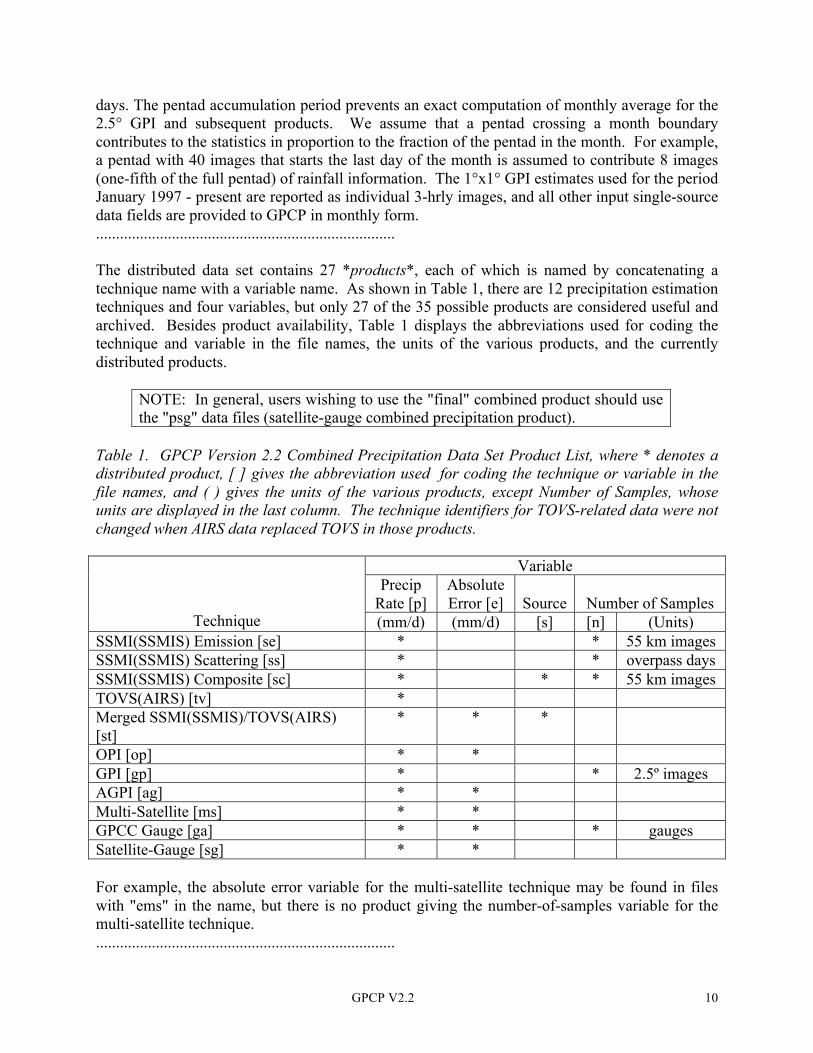
days. The pentad accumulation period prevents an exact computation of monthly average for the 2.5° GPI and subsequent products. We assume that a pentad crossing a month boundary contributes to the statistics in proportion to the fraction of the pentad in the month. For example, a pentad with 40 images that starts the last day of the month is assumed to contribute 8 images (one-fifth of the full pentad) of rainfall information. The 1°x1° GPI estimates used for the period January 1997 - present are reported as individual 3-hrly images, and all other input single-source data fields are provided to GPCP in monthly form. ........................................................................... The distributed data set contains 27 *products*, each of which is named by concatenating a technique name with a variable name. As shown in Table 1, there are 12 precipitation estimation techniques and four variables, but only 27 of the 35 possible products are considered useful and archived. Besides product availability, Table 1 displays the abbreviations used for coding the technique and variable in the file names, the units of the various products, and the currently distributed products.

NOTE: In general, users wishing to use the "final" combined product should use the "psg" data files (satellite-gauge combined precipitation product).

Table 1. GPCP Version 2.2 Combined Precipitation Data Set Product List, where * denotes a distributed product, [ ] gives the abbreviation used for coding the technique or variable in the file names, and ( ) gives the units of the various products, except Number of Samples, whose units are displayed in the last column. The technique identifiers for TOVS-related data were not changed when AIRS data replaced TOVS in those products.

Variable Precip

Rate [p] Absolute Error [e]

Source

Number of Samples

Technique (mm/d) (mm/d) [s] [n] (Units) SSMI(SSMIS) Emission [se] * * 55 km images SSMI(SSMIS) Scattering [ss] * * overpass days SSMI(SSMIS) Composite [sc] * * * 55 km images TOVS(AIRS) [tv] * Merged SSMI(SSMIS)/TOVS(AIRS) [st]

* * *

OPI [op] * * GPI [gp] * * 2.5º images AGPI [ag] * * Multi-Satellite [ms] * * GPCC Gauge [ga] * * * gauges Satellite-Gauge [sg] * * For example, the absolute error variable for the multi-satellite technique may be found in files with "ems" in the name, but there is no product giving the number-of-samples variable for the multi-satellite technique. ...........................................................................

GPCP V2.2 11

The *technique* name tells what algorithm was used to generate the product. There are 12 such techniques in the Version 2.2 Data Set: SSMI (SSMIS) Emission, SSMI (SSMIS) Scattering, SSMI (SSMIS) Composite, TOVS (AIRS), SSMI(SSMIS)/TOVS(AIRS) Composite, OPI, GPI, AGPI, Multi-Satellite, GHCN+CAMS Rain Gauge, GPCC Rain Gauge, and Satellite-Gauge. ........................................................................... The *variable* name tells what parameter is in the product. There are four such variables in the Version 2.2 Data Set: Precipitation Rate, Absolute Error, Source, and Number of Samples. ........................................................................... The *precipitation variable* is computed as described under the individual product headings. All precipitation products have been converted from their original units to mm/d. .......................................................................... The *SSMI (SSMIS) emission precipitation product* is produced by the Polar Satellite Precipitation Data Centre - Emission of the GPCP under the direction of L. Chiu, located at the Department of Geography and GeoInformation Science, George Mason University, Fairfax Virginia, USA, and the Institute of Space and Earth Information Science, Chinese University of Hong Kong, Hong Kong, SAR PRC. The Special Sensor Microwave/Imager (SSMI) and Special Sensor Microwave Imager-Sounder (SSMIS) data are recorded by selected Defense Meteorological Satellite Program satellites, and are provided in packed form by Remote Sensing Systems (RSS; Santa Clara, CA). The algorithm applied is the Wilheit et al. (1991) iterative histogram approach to retrieving precipitation from emission signals in the 19-GHz SSMI channel. It assumes a log-normal precipitation histogram and estimates the freezing level from the 19- and 22-GHz channels. The fit is applied to the full month of data. Individual estimates on the 2.5ºx2.5º grid occasionally fail to converge. In that case the estimate is set to the simple average of the 5º precipitation estimates available in the box for the month. The microwave emission technique infers the quantity of liquid water in a column from the increased low-frequency observed microwave brightness temperatures. Greater amounts of liquid water in the column tend to correlate with greater surface precipitation. The algorithm takes the additional step of fitting a log-normal curve to the month of observations to control sampling-induced noise. This technique works well over ocean where the surface emissivity is low and uniform. Over land, however, the emissivity is near one and extremely heterogeneous, making the scattering algorithm the only choice, so the Wilheit et al. algorithm provides no estimates. The emission product has been uniformly reprocessed using the Version 6 RSS channel brightness temperature data set for the entire SSM/I and SSMIS record. Previously, the archive of emission estimates was processed using Version 4 up through August 2008, then Version 6 thereafter. This change affects ocean and near-coastal ocean regions. Tests showed that the Version 6 emission estimates have unreasonably low values in the tropical maximum-rain areas for months in which sampling is deficient. Three instances are known, all for F08: the first month (July 1987), the partial month after a shutdown (January 1988), and the last month (December 1991). The same problem had occurred in Version 4, and in that case the

GPCP V2.2 12

problematic areas were filled with 5°x5° estimates, which were judged to be reasonable due to their higher sampling. Until this issue is resolved, the Version 6 emission estimates for these three months have been re-scaled using a smoothed version of the field of ratios between Version 4 and Version 6. This approach leaves the light-precipitation areas almost untouched and correctly boosts the values in the high-precipitation areas. The algorithm was retuned for SSMIS to ensure consistency with the SSMI record despite differences in observation strategy and sensor performance. Information on the residual differences will be provided after the provisional status is resolved. The available products related to the SSMI (SSMIS) emission precipitation data are provided in Table 1. ........................................................................... The *SSMI (SSMIS) scattering precipitation product* is produced by the GPCP Polar Satellite Precipitation Data Centre - Scattering under the direction of R. Ferraro, located in the Center for Satellite Applications and Research of the NOAA National Environmental Satellite Data and Information Service (NESDIS/STAR), Washington D.C., USA. The Special Sensor Microwave/Imager (SSMI) and Special Sensor Microwave Imager-Sounder (SSMIS) data are recorded by selected Defense Meteorological Satellite Program satellites, and are transmitted to NESDIS through the Shared Processing System. The algorithm applied is based on the Grody (1991) Scattering Index (SI), supplemented by the Weng and Grody (1994) emission technique in oceanic areas. A similar fall-back approach was used during the period June 1990 - December 1991 when the 85.5-GHz channels were unusable. showed anomalously high coastal values in many locations, and lacked snow screening. The GMDC devised stop-gap fixes pending revisions by the NOAA dataset producers. Pixel-by-pixel retrievals are accumulated onto separate daily ascending and descending 0.333ºx0.333º lat/lon grids, then all the grids are accumulated for the month on the 2.5º grid. The microwave scattering technique infers the quantity of hydrometeor ice in a column from the depressions in the high-frequency 85 GHz channel brightness temperatures. More ice aloft typically implies more surface precipitation. This relationship is physically less direct than in the emission technique, but it works equally well over land and ocean whenever deep convection is important. The algorithm was retuned for SSMIS to ensure consistency with the SSMI record despite differences in observation strategy and sensor performance. Most notably, SSMIS observes at 91 GHz, compared to the 85.5 GHz SSMI channel, so a 91 GHz-based proxy for the 85.5 GHz channel is being used. The SSMIS months are considered “provisional” at this point because the retuning is not yet entirely satisfactory. Also, the entire record of SSMI and SSMIS input data has been quality-controlled more carefully than in previous versions. Information on the residual differences will be provided after the provisional status is resolved. The available products related to the SSMI scattering precipitation data are provided in Table 1. ...........................................................................

GPCP V2.2 13

The *SSMI (SSMIS) composite precipitation product* is produced as part of the GPCP Version 2.2 Combined Precipitation Data Set by the GPCP Merge Development Centre (see Section 2). The concept is to take the SSMI (SSMIS) emission estimate over water and the SSMI (SSMIS) scattering estimate over land. Since the emission technique eliminates land-contaminated pixels individually, a weighted transition between the two results is computed in the coastal zone. The merger is expressed as R(emiss) ; N(emiss) ≥ 0.75 * N(scat)

R(compos) = N(emiss) * R(emiss) + ( N(scat) - N(emiss) ) * R(scat) (1) N(scat) N(emiss) < 0.75 * N(scat) where R is the precipitation rate; N is the number of samples; composite, emiss, and scat denote composite, emission, and scattering, respectively; and the 0.75 threshold allows for fluctuations in the methods of counting samples in the emission and scattering techniques. Note that the second expression reduces to R(scat) when N(emiss) is zero. Important Note: The emission and scattering fields used in this merger have been edited to remove known and suspected artifacts, such as high values in polar regions. These edited fields may be approximated by using the source variable to mask the emission and scattering fields contained in this data set. That is, the user may infer that editing must have occurred for points where the source variable indicates that the scattering or emission (or both) are not used, but the scattering or emission (or both) values are non-missing. The available products related to the SSMI (SSMIS) composite precipitation data are provided in Table 1. ............................................................................ The *TOVS (AIRS) precipitation product* is produced by the Satellite Research Team under the direction of Dr. Joel Susskind, located at NASA Goddard Space Flight Center's Laboratory for Atmospheres, Greenbelt Maryland, USA. In the first part of the data record, data from the Television Infrared Operational Satellite (TIROS) Operational Vertical Sounder (TOVS) instruments aboard the NOAA series of polar-orbiting platforms are processed to provide a host of meteorological statistics. In the second part of the data record, data from the Advanced Infrared Sounder (AIRS) instrument aboard the Earth Observing System Aqua polar-orbiting satellite are processed to provide a host of meteorological statistics. Susskind and Pfaendtner (1989) and Susskind et al. (1997) describe the TOVS data processing, also applied to AIRS. The TOVS precipitation estimates infer precipitation from deep, extensive clouds. The technique uses a multiple regression relationship between collocated rain gauge measurements and several TOVS-based parameters that relate to cloud volume: cloud-top pressure, fractional cloud cover, and relative humidity profile. This relationship is allowed to vary seasonally and latitudinally. Furthermore, separate relationships are developed for ocean and land. The TOVS data are used for the SSMI period July 1987 - April 2005 and are provided at the 1ºx1º, monthly resolution. The data covering the span July 1987 - February 1999 are based on

GPCP V2.2 14

information from two satellites. For the period March 1999 - April 2005, the TOVS estimates are based on information from one satellite due to changes in satellite data format. In addition, the date span 1-17 February 2004 experienced partial (1st and 17th) or total (2-16) loss of TOVS data, so AIRS data are used for February 2004. The AIRS data are available starting in May 2002, are used for the period May 2005 – present, and are provided at the 1ºx1º, monthly resolution. In addition, the date span 1-17 February 2004 experienced partial (1st and 17th) or total (2-16) loss of TOVS data, so AIRS data are used for February 2004. The AIRS precipitation estimates have been bias-adjusted to the TOVS estimates to minimize the TOVS/AIRS data boundary at April/May 2005. Matched histograms of precipitation were computed between the TOVS and AIRS data for the months January, April, July, and October 2004. These seasonal calibrations are applied accordingly to the corresponding seasonal months of data after April 2005. During their periods of use, the TOVS and AIRS estimates are used for filling in the polar and cold-land regions in the SSMI data. The end result is a globally complete "high-quality" precipitation field for use in adjusting the GPI data. The available products related to the TOVS (AIRS) precipitation data are provided in Table 1. ............................................................................ The *merged SSMI(SSMIS)/TOVS(AIRS) precipitation product* is produced as part of the GPCP Version 2.2 Combined Precipitation Data Set by the GPCP Merge Development Centre (see section 2). In the discussion here, “SSMI” and “TOVS” should be understood to include SSMIS and AIRS when those estimates were used. The coverage of the SSMI precipitation estimates is limited by the orbit of the DMSP satellites as well as shortcomings in the microwave technique over cold land. These holes are filled using the globally complete TOVS data. In the nominal latitude span 40°N-S, the SSMI data are used as is. These actual limits on the "as is" band vary over the latitude range 40°-50° North or South depending upon the month of the year. Where there are holes as the result of cold land, the TOVS data are adjusted to the zonally averaged mean bias of the SSMI data and inserted. Just outside of the zone 40ºN-S, the SSMI and TOVS data are averaged using equal weighting. Moving further towards the poles where the SSMI data become less reliable, the SSMI/TOVS average is replaced by TOVS data that have been adjusted to a zonally-averaged presumed bias. In the northern hemisphere, this bias adjustment is anchored on the equatorward side by the zonal average of the SSMI/TOVS values anywhere from 50º-60ºN, depending upon the month of the year. The bias adjustment on the polar side is anchored by the zonal average of the monthly rain gauge data at 70ºN, with a smooth linear variation in between. The gauge's zonal average only includes grid boxes for which the gauge "quality index" (defined in Section 11) is greater than zero. From 70ºN to the North Pole, TOVS data are adjusted to the bias of the same monthly rain gauge value average at 70ºN. The same procedure is applied in the southern hemisphere, except the annual climatological rain gauge values are zonally averaged at 70ºS. The monthly values are not used in the Antarctic as the lack of sufficient land coverage there yields unstable results. Furthermore, the new GPCC analysis lacks data over Antarctica, so this climatological adjustment is from the previous GPCC Monitoring Product. All seasonal variations in this description were developed in off-line

GPCP V2.2 15

studies of typical dataset variations, with the driving criterion being choosing a transition that ensures reasonable performance. The available products related to the merged SSMI/TOVS precipitation data are provided in Table 1. ............................................................................ The *OPI precipitation product* is produced by the Geostationary Satellite Precipitation Data Centre of the GPCP under the direction of Pingping Xie, located in the Climate Prediction Center, NOAA National Centers for Environmental Prediction, Washington D.C., USA. The OPI technique is based on the use of low-Earth orbit satellite outgoing longwave radiation (OLR) observations (Xie and Arkin 1998). Colder OLR radiances are directly related to higher cloud tops, which are related to increased precipitation rates. It is necessary to define "cold" locally, so OLR and precipitation climatologies are computed and a regression relationship is developed for OLR and precipitation anomalies. In use, the total precipitation inferred is the estimated anomaly plus the local climatological value. A backup direct OLR-precipitation regression is used when the anomaly approach yields unphysical values. In this analysis, the precipitation climatology used to develop the OLR-derived precipitation estimates was based on the GPCP Version 2.1 satellite-gauge estimates over the time period 1988-2007. The resulting spatially and temporally varying climatological calibration is then applied to the independent OPI data covering the span 1979-1987 to fill all months lacking SSMI (SSMIS) data. The OPI data for the first two satellites (covering January 1979 through August 1981) were given additional adjustments, described in section 9 under “OPI revisions in 1979-1981” and “OPI revision for October 1985”. This adjusted OPI data provides a globally complete proxy for the SSMI (SSMIS) data. The available products related to the OPI precipitation data are provided in Table 1. ............................................................................ The *GPI precipitation product* is produced by the Geostationary Satellite Precipitation Data Centre of the GPCP under the direction of Pingping Xie, located in the Climate Prediction Center, NOAA National Centers for Environmental Prediction, Washington D.C., USA. Each cooperating geostationary satellite operator (the Geosynchronous Operational Environmental Satellites, or GOES, United States; the Geosynchronous Meteorological Satellite, or GMS, Japan, and subsequently the Ministry of Transportation Satellite, MTSat; and the Meteorological Satellite, or Meteosat, European Community) forward three-hourly "channel 4" ~10.7 micron thermal infrared (IR) imagery to GSPDC. The global IR rainfall estimates are then generated from a merger of these data using the GOES Precipitation Index (GPI; Arkin and Meisner, 1987) technique, which relates cold cloud-top area to rain rate. The GPI technique is based on the use of geostationary satellite IR observations. Colder IR brightness temperatures are directly related to higher cloud tops, which are loosely related to increased precipitation rates. From the GATE data, an empirical relationship between brightness temperature and precipitation rate was developed. For a brightness temperature ≤ 235K, a rain rate of 3 mm/hour is assigned. For a brightness temperature > 235K, a rain rate of 0 mm/hour is

GPCP V2.2 16

assigned. The GPI works best over space and time averages of at least 250 km and 6 hours, respectively, in oceanic regions with deep convection. For the period 1986-March 1998 the GPI data are accumulated on a 2.5ºx2.5º lat/lon grid for pentads (5-day periods), preventing an exact computation of the monthly average. We assume that a pentad crossing a month boundary contributes to the statistics in proportion to the fraction of the pentad in the month. For example, given a pentad that starts the last day of the month, 0.2 (one-fifth) of its samples are assigned to the month in question and 0.8 (four-fifths) of its samples are assigned to the following month. Starting with October 1996 the GPI data are accumulated on a 1ºx1º lat/lon grid for individual 3-hrly images. In this case monthly totals are computed as the sum of all available hours in the month. The Version 2.2 GPI product is based on the 2.5°x2.5° IR data for the period 1988-1996, and the 1ºx1º beginning in 1997. In both data sets gaps in geo-IR are filled with low-earth-orbit IR (leo-IR) data from the NOAA series of polar orbiting meteorological satellites. However, the 2.5ºx2.5º data only contain the leo-IR used for fill-in, while the 1ºx1º data contain the full leo-IR. The latter allows a more accurate AGPI (see "AGPI precipitation product"). The Indian Ocean sector routinely lacked geo-IR coverage until Meteosat-5 was repositioned to that region in June 1998. See the "IR data correction" and "known data set issues" sections for some additional details on the GPI data record. The available products related to the GPI precipitation data are provided in Table 1. ........................................................................... The *AGPI precipitation product* is produced as part of the GPCP Version 2.2 Combined Precipitation Data Set by the GPCP Merge Development Centre (see section 2). The technique follows the Adler et al. (1994) Adjusted GPI (AGPI). During the SSMI (SSMIS) period (starting July 1987), separate monthly averages of approximately coincident GPI and merged SSMI/TOVS precipitation estimates (which also include SSMIS and AIRS) are formed by taking cut-outs of the 3-hourly GPI values that correspond most closely in time to the local overpass time of the DMSP platform. The ratio of merged SSMI/TOVS to GPI averages is computed and controlled to prevent unstable answers. In regions of light precipitation an additive adjustment is computed as the difference between smoothed merged SSMI/TOVS and ratio-adjusted GPI values when the merged SSMI/TOVS is greater, and zero otherwise. The spatially varying arrays of adjustment coefficients are then applied to the full set of GPI estimates. In regions lacking geo-IR data, leo-GPI data are calibrated to the merged SSMI/TOVS, then these calibrated leo-GPI are calibrated to the geo-AGPI. This two-step process tries to mimic the information contained in the AGPI, namely the local bias of the SSMI and possible diurnal cycle biases in the geo-AGPI. The second step can be done only in regions with both geo- and leo-IR data, and then smooth-filled across the leo-IR fill-in. In the case of the 2.5ºx2.5º IR, which lacks leo-IR in geo-IR regions, the missing

GPCP V2.2 17

calibrated leo-GPI is approximated by smoothed merged SSMI/TOVS for doing the calibration to geo-AGPI. During the pre-SSMI period (January 1986 - June 1987 and December 1987), the OPI data, as calibrated by the GPCP satellite-gauge estimates for part of the SSMI period (1988-2007), are used as a proxy for the merged SSMI/TOVS field in the AGPI procedure described for the SSMI period. Because the overpass times of the calibrated OPI data are not available, a controlled ratio between the full monthly calibrated OPI estimates and the full monthly GPI data is computed. These ratios are then applied to the GPI data to form the AGPI. The additive constant is computed and applied, when necessary, for light-precipitation regions. During the pre-SSMI period January 1979 - December 1985 there is no geo-IR GPI, and therefore no AGPI. The OPI data, calibrated by the GPCP satellite-gauge estimates for the same part of the SSMI period (1988-2007), are used "as is" for the multi-satellite estimates. The available products related to the AGPI precipitation data are provided in Table 1. ........................................................................... The *multi-satellite precipitation product* is produced as part of the GPCP Version 2.2 Combined Precipitation Data Set by the GPCP Merge Development Centre (see section 2) following Huffman et al. (1995). During the SSMI period (which includes SSMIS), the multi-satellite field as used in the satellite-gauge combination product (SG) consists of a combination of Geo-AGPI estimates where available (latitudes 40ºN-S), the weighted combination of the merged SSMI/TOVS estimates and the leo-AGPI elsewhere in the 40ºN-S belt, and the merged SSMI/TOVS data outside of that zone. Note that “TOVS” includes AIRS where that data replaced the TOVS estimates. The combination weights are the inverse (estimated) error variances of the respective estimates. Such weighted combination of SSMI/TOVS and leo-AGPI is done because the leo-IR lacks the sampling to support the full AGPI adjustment scheme. After use in the SG, the final version of the multi-satellite product is generated by calibrating the multi-satellite field to the SG, in parallel with the scheme used to calibrate the OPI to the SG. This step is necessary to ensure consistency between the two approaches, and was added to GPCP processing 20 June 2006. During the pre-SSMI January 1986 - June 1987 and December 1987, the multi-satellite field consists of a combination of geo-AGPI estimates where available (latitudes 40ºN-S) and the calibrated OPI estimates elsewhere. The combination weights are the inverse (estimated) error variances of the respective estimates. During the pre-SSMI period January 1979 - December 1985, the OPI data, calibrated by the GPCP satellite-gauge estimates, are used "as is" for the multi-satellite estimates. The available products related to the multi-satellite precipitation data are provided in Table 1. ........................................................................... The *rain gauge precipitation product* for the period 1979 - present is produced by the Global Precipitation Climatology Centre (GPCC) under the direction of Andreas Becker and Udo

GPCP V2.2 18

Schneider, located in the Deutscher Wetterdienst, Offenbach a.M., Germany (Schneider et al. 2008). [Note: Throughout, we are clearly dealing with all forms of precipitation, but we follow the customary practice here of referring to precipitation gauges as “rain gauges”.] Rain gauge reports are archived from a time-varying collection of over 70,000 stations around the globe, both from Global Telecommunications System (GTS) reports and from other world-wide or national data collections. An extensive quality-control system is run, featuring an automated screening and then a manual step designed to retain legitimate extreme events that characterize precipitation. This long-term data collection and preparation activity feeds into an analysis that is done in two steps. First, a long-term climatology is assembled from all available gauge data, focusing on the period 1951-2000. The lack of complete consistency in period of record for individual stations has been shown to be less important than the gain in detail, particularly in complex terrain. Then for each month, the individual gauge reports are converted to deviations from climatology, and are analyzed into gridded values using a variant of the SPHEREMAP spatial interpolation routine (Willmott et al. 1985). Finally, the month’s analysis is produced by superimposing the anomaly analysis on the month’s climatology. The GPCC creates multiple products, and two are used in the GPCP Version 2.2. The Full Data Reanalysis (currently Version 5) is a retrospective analysis that covers the period 1901-2009, and it is used in GPCP for the span 1979-2009. Thereafter we use the GPCC Monitoring Product (currently Version 3), which has a similar quality control and the same analysis scheme as the Full Data Reanalysis, but whose data source is limited to GTS reports. Compared to Version 2, the advantages of using GPCC data throughout are that 1) we no longer need to use the separate and differently prepared gauge analysis based on the Global Historical Climate Network and Climate Analysis and Monitoring System (GHCN+CAMS) for the period 1979-1985, as we did for Version 2, and 2) the numbers of gauges used are much higher for much of the period of record. When the Full Data Reanalysis is updated to a longer record we expect to reprocess the GPCP datasets to take advantage of the improved data. We continue the GPCP’s long-standing practice of correcting all gauge analysis values for climatological estimates of systematic error due to wind effects, side-wetting, evaporation, etc., following Legates [1987]. We hope to develop a more modern and detailed correction for these effects in subsequent versions. The available products related to the rain gauge precipitation data are provided in Table 1. ........................................................................... The *satellite-gauge precipitation product* is produced as part of the GPCP Version 2.2 Combined Precipitation Data Set by the GPCP Merge Development Centre (see section 2) in two steps (Huffman et al. 1995). Note the subtle point that the multi-satellite (MS) data used here is the original, in which climatological gauge scaling is approximately included during the pre-SSMI era, but not during the SSMI era. 1a. For each grid box that has less than 65% water coverage on a 5x5-gridbox template: 1b. Average the gauge and MS estimates separately on a 5x5-gridbox template centered on the

box of interest, or a 7x7-gridbox area if there is "too little" data. 1c. Compute the weighted-average gauge to weighted-average MS ratio, 1d. controlling the maximum ratio to be 2 for the weighted-average MS in the range [0,7]

mm/d, 1.25 above 17 mm/d, and linearly tapered in between to suppress artifacts.

GPCP V2.2 19

1e. When the ratio exceeds the limit, compute an additive adjustment that is capped at 1.7 mm/d at zero weighted-average MS and linearly tapers to zero at 7 mm/d. This is intended to account for the MS badly missing light precipitation.

1f. For all areas with smoothed fractional coverage by water greater than 65%, the ratio is set to one and the additive adjustment is set to zero.

1g. In each grid box, whether or not there was any adjustment, the gauge-adjusted MS is the product of the MS and the ratio, added to the additive adjustment.

1h. In each grid box, whether or not there was any adjustment, the estimated random errors for both gauge and gauge-adjusted MS are recomputed, using the straight average of the two as the estimated precipitation value for both calculations. This step prevents inconsistent results that arise when the random errors are computed with individual precipitation values that are not close to each other.

2. In each grid box, whether or not there was any adjustment in step 1, the gauge-adjusted MS and gauge values are combined in a weighted average, where the weights are the recomputed inverse (estimated) error variances to form the Satellite-Gauge combination product.

The available products related to the satellite-gauge precipitation data are provided in Table 1. ........................................................................... The *random error* is produced as part of the GPCP Version 2.2 Combined Precipitation Data Set by the GPCP Merge Development Centre (see section 2). Following Huffman (1997a), bias error is neglected compared to random error (both physical and algorithmic), then simple theoretical and practical considerations lead to the functional form VAR = H * ( rbar + S) * [ 24 + 49 * SQRT ( rbar ) ] (2) Ni for absolute random error, where VAR is the estimated error variance of an average over a finite set of observations, H is taken as constant (actually slightly dependent on the shape of the precipitation rate histogram), rbar is the average precipitation rate in mm/d, S is taken as constant (approximately SQRT(VAR) for rbar=0), Ni is the number of independent samples in the set of observations, and the expression in square brackets is a parameterization of the conditional precipitation rate based on work with the Goddard Scattering Algorithm, Version 2.1 (Adler et al. 1994) and fitting of (2) to the Surface Reference Data Center analyses (McNab 1995). The "constants" H and S are set for each of the data sets for which error estimates are required by comparison of the data set against the SRDC and GPCC analyses and tropical Pacific atoll gauge data (Morrissey and Green 1991). The computed value of H actually accounts for multiplicative errors in Ni and the conditional rainrate parameterization (the [ ] term), in addition to H itself. Table 2 shows the numerical values of H and S. All absolute random error fields have been converted from their original units of mm/mo to mm/d.

GPCP V2.2 20

Table 2. Numerical values of H and S constants used to estimate absolute error for various precipitation estimates.

Technique S (mm/d) H

SSMI(SSMIS) Emission [se] 1 3 (55 km images) SSMI(SSMIS) Scattering [ss] 1 3.2 (55 km images) TOVS(AIRS) [tv] 1 0.0045 OPI [op] 1 0.0045 AGPI [ag] 0.5 0.45 (2.5° images) Rain Gauge [ga] 0.267 0.0075 (gauges)

For the independent data sets rbar is taken to be the independent estimate of rain itself. However, when these errors are used in the combination, theory and tests show that the result is a low bias. Rbar needs to have the same value in all the error estimates; so we estimate it as the simple average of all rainfall values contributing to the combination. Note that this scheme is only used in computing errors used in the combination. The formalism mixes algorithm and sampling error, and should be replaced by a more complete method when additional information is available from the single-source estimates. However, when Krajewski et al. (2000) developed and applied a methodology for assessing the expected random error in a gridded precipitation field, their estimates of expected error agree rather closely with the errors estimated for the multi-satellite and satellite-gauge combinations. ........................................................................... The *source variable* is produced as part of the GPCP Version 2.2 Combined Precipitation Data Set by the GPCP Merge Development Centre (see section 2). It is available for the SSMI(SSMIS) composite and the merged SSMI(SSMIS)/TOVS(AIRS) techniques and gives the fractional contribution to the composite by the SSMI (SSMIS) scattering estimate. Referring to (1) in the "SSMI(SSMIS) composite precipitation product" description, the SOURCE may be expressed as 0 ; N(emiss) ≥ 0.75 * N(scat)

SOURCE = ( N(scat) - N(emiss) ) N(emiss) < 0.75 * N(scat) (3) N(scat)

N(SSMI) + 2 ; merged SSMI(SSMIS)/TOVS(AIRS)

4 ; TOVS(AIRS) where N is the number of samples, emiss and scat denote SSMI(SSMIS) emission and scattering, respectively, N(SSMI) is the SSMI(SSMIS) source determined from the emission and scattering components, and the 0.75 threshold allows for fluctuations in the methods of counting samples in the emission and scattering techniques. Note that the second expression reduces to 1 when N(emiss) is zero. ...........................................................................

GPCP V2.2 21

The *number of samples variable* is produced in a variety of units as described under the individual product headings. ........................................................................... The *SSMI(SSMIS) emission number of samples product* is provided to the GPCP as the number of pixels contributing to the grid box average for the month (i.e., the number of "good" pixels). As part of the Version 2.2 Data Set processing, this number is converted to the number of 55x55 km boxes that the number of pixels can evenly and completely cover. This conversion provides a very approximate (over)estimate of the number of independent samples contributing to the average. The available products related to the SSMI(SSMIS) emission number of samples are provided in Table 1. ........................................................................... The *SSMI(SSMIS) scattering number of samples product* is provided to the GPCP as the number of "overpass days," the count of days in the month that had at least one ascending pass plus days that had at least one descending pass. As part of the Version 2.2 Data Set processing, this number is converted to the number of 55x55 km boxes that the number of pixels can evenly and completely cover. This conversion provides a very approximate (over)estimate of the number of independent samples contributing to the average. The available products related to the SSMI(SSMIS) scattering number of samples are provided in Table 1. ........................................................................... The *SSMI(SSMIS) composite number of samples product* is produced as part of the GPCP Version 2.2 Combined Precipitation Data Set by the GPCP Merge Development Centre (see section 2). Due to the different units for the SSMI emission and scattering numbers of samples, it is necessary to convert at least one before doing the merger. We have chosen to convert overpass days (SSMI(SSMIS) scattering estimates) to an estimate of complete 55x55 km boxes (our modified units for the SSMI(SSMIS) emission). In the latitude belt 60°N-S, orbits in the same direction don't overlap on a single day, and there is an approximate linear relationship between overpass days and 55 km boxes. Outside that belt the overlaps cause non-linearity, but we ignore it because the general lack of reliable SSMI(SSMIS) at higher latitudes overwhelms details about the numbers of samples. The separate numbers of samples for each technique, measured in 55-km boxes, are merged according to the same formula as the rainfall: N(emiss) ; N(emiss) ≥ 0.75 * N(scat)

N(compos) = N(emiss) * N(emiss) + ( N(scat) - N(emiss) ) * N(scat) (4) N(scat) N(emiss) < 0.75 * N(scat) where N is the number of samples; composite, emiss, and scat denote composite, emission, and scattering, respectively; and the 0.75 threshold allows for fluctuations in the methods of counting samples in the emission and scattering techniques. Note that the second expression reduces to N(scat) when N(emiss) is zero. The available products related to the SSMI(SSMIS) composite number of samples are provided in Table 1. ...........................................................................

GPCP V2.2 22

The *GPI number of samples product* is provided to the GPCP as the number of IR images that contribute to the 2.5ºx2.5º grid box. For the 2.5ºx2.5º IR data it is provided as the number of images per pentad (5-day period), while for the 1ºx1º IR data each 3-hrly image is a separate dataset. For the 2.5ºx2.5º IR data the contribution by pentads that cross month boundaries are taken to be proportional to the fraction of the pentad in the month.to the fraction of the pentad in the month. For example, given a pentad that starts the last day of the month, 0.2 (one-fifth) of its samples are assigned to the month in question and 0.8 (four-fifths) of its samples are assigned to the following month. The available products related to the GPI number of samples are provided in Table 1. .......................................................................... The *rain gauge number of samples product* is provided to the GPCP as the number of stations providing gauge reports for the month in the 2.5ºx2.5º grid box. The available products related to the rain gauge number of samples are provided in Table 1. .......................................................................... The *units of the variables* are given in Table 1 (Section 5) under the entry "Products." In particular, the precipitation estimates are in mm/day. .......................................................................... 6. Temporal and Spatial Coverage and Resolution The *date* for a file is the year in which the months it contains occurred. The date for a grid is the year/month over which the observations were accumulated to form the averages and estimates. All dates are UTC. ........................................................................... The *temporal resolution* of the products is one calendar month. The temporal resolution of the original single-source data sets is also one month, except the GPI data source has pentad (five-day) or 3-hourly temporal resolution for the 2.5°x2.5° and 1°x1° IR data sets, respectively. Some of the single-source data sets are available from other archives at a finer resolution. ........................................................................... The *period of record* for the GPCP Version 2.2 Combined Precipitation is January 1979 through the present, delayed a few months for data collection and processing. The start is based on the availability of the OLR data. The end is based on the availability of input analyses, and is extended as complete sets of new data arrive. Some of the single-source data sets have longer periods of record in their original archival sites. The data span for each product available in the distributed data set is provided in Table 3. Some products are available for longer timespans, but only the data used in the GPCP Version 2.2 processing is distributed. Data available but not used in the GPCP Version 2.2 processing are available upon request from the data set creators.

Table 3. GPCP Version 2.2 Combined Precipitation Data Set Product List with data span coverage in the distributed data set.

Technique/Variable Availability in Distribution

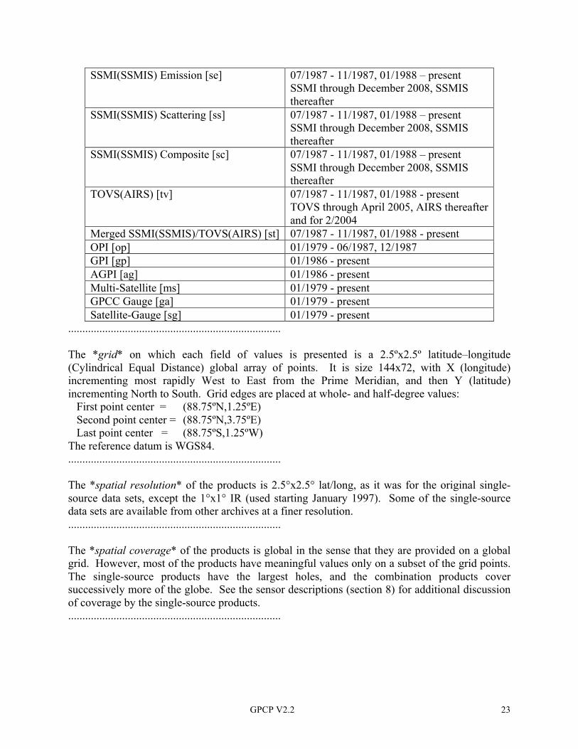
GPCP V2.2 23

SSMI(SSMIS) Emission [se] 07/1987 - 11/1987, 01/1988 – present SSMI through December 2008, SSMIS thereafter

SSMI(SSMIS) Scattering [ss] 07/1987 - 11/1987, 01/1988 – present SSMI through December 2008, SSMIS thereafter

SSMI(SSMIS) Composite [sc] 07/1987 - 11/1987, 01/1988 – present SSMI through December 2008, SSMIS thereafter

TOVS(AIRS) [tv] 07/1987 - 11/1987, 01/1988 - present TOVS through April 2005, AIRS thereafter and for 2/2004

Merged SSMI(SSMIS)/TOVS(AIRS) [st] 07/1987 - 11/1987, 01/1988 - present OPI [op] 01/1979 - 06/1987, 12/1987 GPI [gp] 01/1986 - present AGPI [ag] 01/1986 - present Multi-Satellite [ms] 01/1979 - present GPCC Gauge [ga] 01/1979 - present Satellite-Gauge [sg] 01/1979 - present

........................................................................... The *grid* on which each field of values is presented is a 2.5ºx2.5º latitude–longitude (Cylindrical Equal Distance) global array of points. It is size 144x72, with X (longitude) incrementing most rapidly West to East from the Prime Meridian, and then Y (latitude) incrementing North to South. Grid edges are placed at whole- and half-degree values: First point center = (88.75ºN,1.25ºE) Second point center = (88.75ºN,3.75ºE) Last point center = (88.75ºS,1.25ºW) The reference datum is WGS84. ........................................................................... The *spatial resolution* of the products is 2.5°x2.5° lat/long, as it was for the original single-source data sets, except the 1°x1° IR (used starting January 1997). Some of the single-source data sets are available from other archives at a finer resolution. ........................................................................... The *spatial coverage* of the products is global in the sense that they are provided on a global grid. However, most of the products have meaningful values only on a subset of the grid points. The single-source products have the largest holes, and the combination products cover successively more of the globe. See the sensor descriptions (section 8) for additional discussion of coverage by the single-source products. ...........................................................................

GPCP V2.2 24

7. Production and Updates The GPCP is responsible for managing *production and updates* of the GPCP Combined Precipitation Data Set (WCRP 1986). Version 2.2 is produced by the GPCP Merge Development Centre (GMDC), located at NASA Goddard Space Flight Center in the Laboratory for Atmospheres. Various groups in the international science community are given the tasks of preparing precipitation estimates from individual data sources, then the GMDC is charged with combining these into a "best" global product. This activity takes place after real time, at a pace governed by agreements about forwarding data to the individual centers and activities designed to ensure the quality in each processing step, and usually happens within three months. The techniques used to compute the individual and combination estimates are described in section 5. Updates will be released to (1) extend the data record, (2) take advantage of improved input data sets and combination techniques, or (3) correct errors. Updates resulting from the last two cases will be given new version numbers.

NOTE: The changes described in this section are typical of the changes that are required to keep the GPCP Combined Precipitation Data Set abreast of current requirements and science. Users are strongly encouraged to check back routinely for additional upgrades, and to refer other users to this site rather than redistributing data that are potentially out of date.

.......................................................................... The upgrade from Version 2 to Version 2.1 included the following *data set revisions*: 1. The GPCC analyses used replaced a combination of the March 1999 version of the

GHCN+CAMS data for the period January 1979 – December 1985, the January 1999 version of the GPCC Monitoring analysis for 1986-September 1998, and real-time pulls from the GPCC of Monitoring analyses for subsequent months.

2. The OPI calibration was changed from using GPCP Version 2 for the period 1988-1995 to using GPCP Version 2.1 for the period 1988-2007.

3. The extra adjustment to the first two satellites’ OPI (January 1979 through August 1981) was recomputed using Version 2.1 and the GPCC Full Data Reanalysis, versus the previous Version 2 and GHCN+CAMS.

4. The date span 1-17 February 2004 experienced partial (1st and 17th) or total (2-16) loss of TOVS data, so AIRS data are used for February 2004 in Version 2.1.

5. The 5°x5° SSMI emission-based estimates (i.e., over ocean) for July 1990 – December 1991 were loaded, completing the 5°x5° time series for use as fill-in when the usual 2.5°x2.5° product failed to converge.

6. Corrections were made by CPC in the mid-Pacific overlap region between geo-IR satellites for October and November 1994.

7. Accumulated minor corrections to the input data sets since the Version 2 computation were applied in Version 2.1.

GPCP V2.2 25

To date, these data set revisions have been implemented from Version 2.1 to Version 2.2: 1. CCW emission estimates have been uniformly reprocessed using the Version 6 Remote

Sensing Systems (RSS) channel brightness temperature data set for the entire SSMI and SSMIS record. Previously, the archive of CCW estimates was processed using Version 4 up through August 2008, then Version 6 thereafter. This change affects ocean and near-coastal ocean regions. Tests showed that the CCW Version 6 estimates have unreasonably low values in the tropical maximum-rain areas for months in which sampling is deficient. Three instances are known, all for F08: the first month (July 1987), the partial month after a shutdown (January 1988), and the last month (December 1991). The same problem had occurred in Version 4, and in that case the problematic areas were filled with 5°x5° estimates, which were judged to be reasonable due to their higher sampling. Until this issue is resolved, the Version 6 estimates for these three months have been re-scaled using a smoothed version of the field of ratios between Version 4 and Version 6. This approach leaves the light-precipitation areas almost untouched and correctly boosts the values in the high-precipitation areas.

2. NOAA scattering estimates have been uniformly reprocessed with enhanced quality control (QC) for the entire SSMI record. This had the effect of reducing the global-average land precipitation average because many of the defects indentified in the QC resulted in precipitation artifacts, and the time series of new values over land is more consistent with the time series of the GPCC Version 5 Full Gauge Analysis Product (see next paragraph). This change affects land, coasts, and near-coastal ocean regions. However, given the strong control that the gauge analysis exerts in most land regions, the principal effect appears in islands, coasts, and near-coastal regions. Recall that bias adjustments of the multi-satellite product to the gauge analysis do not affect smaller islands and peninsulas, so these regions are more sensitive to changes in the NOAA scattering estimates. At the same time, the alternative PR2 precipitation estimates used during the period June 1990 – December 1991, when the 85 GHz channels were out on the F08 SSMI, showed anomalously high coastal values in many locations, and lacked snow screening. The GMDC devised stop-gap fixes until the NOAA dataset producers can provide revisions.

3. The GPCC gauge precipitation analysis has been reprocessed to extend the Version 5 Full Analysis through 2009, and use the Version 3 Monitoring Analysis thereafter. These changes are typically small, although regions with sparse gauge coverage may show appreciable differences. This change affects land and coasts, but with less impact in smaller islands and peninsulas.

4. The F17 SSMIS was introduced as the calibrating microwave data source to replace the F13 SSMI, which failed in September 2009. F17 was chosen from the available SSMIS datasets (F16, F17, or F18) due to its stable orbit and local overpass time just a half hour ahead of the 6 a.m./p.m. local time that has typified the previous calibrators (F08, F11, and F13). The start of F17 data is set at January 2009 to simplify tracking possible artifacts associated with the change of calibrator. Maintaining continuity with the previous SSMI sensors, the CCW estimates are computed with RSS channel brightness temperatures and the NOAA estimates are based on Fleet Numerical Meteorological and Oceanographic Center (FNMOC) data. All of the SSMIS datasets have had substantial calibration issues, and the current adjustments are still not entirely satisfactory. This problem is most acute for the NOAA algorithm, which depends on the high frequencies. As well, the QC mentioned above has not yet been applied

GPCP V2.2 26

to F17. Pending resolution of these issues, a simple scaling is being done to make the NOAA F17 estimates for 2009 as consistent as possible with corresponding NOAA F13 estimates: For each 2.5° grid box the precipitation for each dataset is separately accumulated for the nine months of overlapping data, January 2009 – September 2009, then smoothed with a 3x3 gridbox boxcar filter. The ratio F13/F17 is taken as the adjustment for all months of F17 estimates (January 2009 – December 2010). The CCW estimates seem little affected by the SSMIS calibration issues, although changes in the scan strategies between SSMI and SSMIS required some adjustments to the algorithm. The most noticeable differences occur in mid-latitudes.

5. Other input estimates, including the Outgoing Longwave Radiation (OLR) Precipitation Index (OPI), Television-Infrared Optical Sensor (TIROS) Operational Vertical Sounder (TOVS), and Advanced Infrared Sounder (AIRS) have not been changed, although the various calibrations applied to them may adjust the values seen in the GPCP SG.

Until the NOAA F17 dataset issues are resolved, the months of GPCP SG data involving F17, namely January 2009 – present, will be labeled “provisional”. This labeling indicates that the developers believe the data for these months to be useful, but that users should exercise caution in cross-checking unexpected features. This is particularly the case for coasts, near-coastal ocean regions, islands, and small peninsulas, which are less likely to have the gauge coverage necessary to control possible biases in the F17 and F08 PR2 estimates. The initial release will extend the data set through the end of 2010, with further extension to the (delayed) present soon thereafter. Work continues on revising the GPCP One-Degree Daily (1DD) algorithm to use F17, while the GPCP Pentad dataset has not yet been rescaled to accommodate the new GPCP SG. .......................................................................... A number of *known data set issues* exist: 1. The present GPI contains no intersatellite calibration. This is not a serious issue in the AGPI

and combination, although having the intersatellite calibration would provide a better GPI and at second order refine the AGPI at satellite data boundaries. By contrast, the "official" NCEP GPI time series has intersatellite calibration for Jan. 1986 - March 1998, then none thereafter. Tests show that the 40ºN-S oceanic average GPI is about 3% higher for the intercalibrated data, compared to the non-intercalibrated data.

2. The present GPI has a 3x3-gridbox smoother applied for non-SSMI months (Jan. 1986 - June 1987, Dec. 1987). Locally, values are different than the non-smoothed version, but large-area averages should be accurate.

3. Presently the choice of IR satellite source is strictly by the number of images in the 2.5ºx2.5º 3-hrly pentad IR (used to compute adjustment coefficients), but in the 2.5ºx2.5º pentad IR the distance to the satellite is also considered (used to compute the AGPI). So, at some locations nearly equidistant between the two satellites the AGPI is derived for one satellite, but applied to the other. NOTE: In the 1ºx1º 3-hrly GPI it is possible for the two satellites to cut in and out on successive hours. As long as the relative contribution of each is in the same proportion for

GPCP V2.2 27

both the SSMI-matched subset and the full data set this is not too important. Using inter-satellite calibrated data would overcome this issue, although it is likely a second-order effect.

4. The 1ºx1º IR dataset provides comprehensive leo-IR data while the 2.5ºx2.5º IR only provides leo-IR in regions lacking geo-IR. The additional data in the 1ºx1º IR allows more accuracy in estimating the calibration of the SSMI-calibrated leo-GPI to the geo-AGPI, causing biases between the 1ºx1º and 2.5ºx2.5º AGPI in leo regions (the Indian Ocean being the prime case) of up to 15% in the previous Version 1c. NOTE: Alternatively, a whole different 2.5ºx2.5º pentad low-orbit GPI dataset could be generated, and then integrated into the system. The improvement over the fix should be only second-order.

5. The GMS 2.5ºx2.5º histograms were collected with temperature bin boundaries at half-degree values, but the 1ºx1º histograms are being collected on whole-degree temperature boundaries; this causes GPI differences in excess of 10% at 30-40º latitude, and everywhere the 1ºx1º GPI is smaller. The AGPI largely calibrates out this problem, but if the GPI itself needs to be consistent, the 235K class could be split in the 1ºx1º histograms in a future release.

6. The SSMIS precipitation estimates use a proxy 85 GHZ channels based on the 91 GHz channels, calibrated to approximately match the zonal average TOVS using the months January, April, July, and October 2004 as the seasonal calibration months, but regional differences remain.

7. Beginning with January 2009, SSMIS precipitation estimates replaced the SSMI estimates because the F13 SSMI failed in September 2009 and we wanted to both avoid possible degraded performance and to establish a whole-year data boundary to aid in diagnosing possible biases. The SSMIS data have been adjusted to match the large-scale bias of the SSMI to maintain homogeneity across the data boundary. For simplicity, any distributed dataset that depends on SSMI before January 2009 utilizes SSMIS data in place of the SSMI starting with that month. This applies to the datasets ending in “se”, “ss”, “sc”, “st", "ms", and "sg".

8. The TOVS precipitation estimates for the SSMI period July 1987 – February 1999 are based on two satellites. For February 1999 – April 2005, the TOVS estimates are based on only one satellite.

9. TOVS data were partially denied for the period 10-18 September 2001 and cannot be recovered. As well, various operational issues caused partially or completely missing days of TOVS data, particularly in the last few months of NOAA-14’s useful life. In a future reprocessing, partial and completely missing days will be replaced with AIRS data during the overlap period, May 2002 – April 2005.

10. The AIRS precipitation estimates are calibrated to approximately match the zonal average TOVS using the months January, April, July, and October 2004 as the seasonal calibration months, but regional differences remain.

11. Beginning with May 2005, AIRS precipitation estimates replaced the TOVS estimates at high latitudes because of TOVS instrument termination. The AIRS data has been adjusted to match the large-scale bias of the TOVS to maintain homogeneity across the data boundary. For simplicity, any distributed dataset that depends on TOVS before May 2005 utilizes AIRS data in place of the TOVS starting with that month. This applies to the datasets ending in "st", "tv", "ms", and "sg".

GPCP V2.2 28

12. Every effort has been made to preserve the homogeneity of the Version 2.2 data record. However, the regional variances inherent in the OPI data are typically smaller than those encountered in the SSMI data, so the statistical nature of the Version 2.2 fields will be different for the pre-SSMI and SSMI eras. Future efforts will be directed at minimizing these differences.

13. The rain gauge data used in the Version 2.2 analysis consists of GPCC Full for the period 1979-2009 and GPCC Monitoring for the period January 2010 - present. Though there is strong consistency in analysis scheme, quality control, and data sources between the two analyses, there exists a minimal possibility of a discernible boundary at the cross-over month for the land precipitation.

14. Every attempt has been made to create an observation-only based precipitation data set. However, the TOVS estimates (but not AIRS) rely on numerical model data to initialize the estimation technique. It is believed that the impact of the numerical model data is minimal on the final precipitation estimates.

15. Some polar-orbiting satellites can experienced significant drifting of the equator-crossing time during their period of service. There is no direct effect on the accuracy of the data, but it is possible that the systematic change in sampling time could introduce biases in the resulting precipitation estimates. It is unlikely that this issue affects the SSMI(SSMIS) data used for calibration because the sequence of single satellites used have all stayed within ±1 hour of the nominal 6 a.m. / 6 p.m. overpass time.

16. The new GPCC climatology/anomaly analysis scheme is intended to perform well where data are sparse and/or the terrain is complex. Nonetheless, testing remains to show this everywhere.

........................................................................... 8. Sensors The Special Sensor Microwave/Imager (*SSMI*) is a multi-channel passive microwave radiometer that has flown on selected Defense Meteorological Satellite Program (DMSP) platforms since mid-1987. The DMSP is placed in a sun-synchronous polar orbit with a period of about 102 min. The SSMI provides vertical and horizontal polarization values for 19, 22, 37, and 85.5 GHz frequencies (except only vertical at 22) with conical scanning. Pixels and scans are spaced 25 km apart at the suborbital point, except the 85.5-GHz channels are collected at 12.5 km spacing. Every other high-frequency pixel is co-located with the low-frequency pixels, starting with the first pixel in the scan and the first scan in a pair of scans. The channels have resolutions that vary from 12.5x15 km for the 85.5 GHz (oval due to the slanted viewing angle) to 60x75 km for the 19 GHz. The polar orbit provides nominal coverage over the latitudes 85ºN-S, although limitations in retrieval techniques prevent useful precipitation estimates in cases of cold land (scattering), land (emission), or sea ice (both scattering and emission). The SSMI is an operational sensor, so the data record suffers the usual gaps in the record due to processing errors, down time on receivers, etc. Over time the coverage has improved as the operational system has matured. As well, the first 85.5 GHz sensor to fly degraded quickly due

GPCP V2.2 29

to inadequate solar shielding. After launch in mid-1987, the 85.5 GHz vertical- and horizontal-polarization channels became unusable in 1989 and 1990, respectively. Further details are available in Hollinger et al. (1990). The SSMI emission estimates are based on data from the F08 instrument from mid-1987 through 1991, with the F11 being used for 1992 through April 1995, and the F13 for May 1995 through December 2008. ........................................................................... The Special Sensor Microwave Imager/Sounder (*SSMIS*) is a multi-channel passive microwave radiometer that has flown on selected Defense Meteorological Satellite Program (DMSP) platforms since late 2003. The DMSP is placed in a sun-synchronous polar orbit with a period of about 102 min. The SSMIS provides vertical and horizontal polarization values for the SSMI-like 19, 22, 37, and 91 GHz frequencies (except only vertical at 22) with conical scanning, as well as other channels with a heritage in the Special Sensor Microwave/Temperature 2 (SSM/T2) sensor. Unlike SSMI, every SSMIS scan observes at all channels: pixels and scans are spaced 25 and 12.5 km apart at the suborbital point for channels below 91 GHz, 12.5 km for both pixel and scans for 91 GHz. Thus, the high-frequency channels have twice as many footprints per scan as the lower-frequency channels. Separate feed horns are used for 91 GHz and the rest of the SSMI-like frequencies, so there is not a 1:1 co-location of channel values, as there is for SSMI. The SSMI-like channels have the resolutions

46.5x73.6 km (19, 22 GHz) 31.2x45.0 km (37 GHz) 13.2x15.5 km (91 GHz)

with the slanted viewing angle and in-line processing determining the oval shape. A summary of the processing necessary to enable use of the SSMIS is being developed. The polar orbit provides nominal coverage over the latitudes 85ºN-S, although limitations in current retrieval techniques prevent useful precipitation estimates in cases of cold land (scattering), land (emission), or sea ice (both scattering and emission). The SSMIS is an operational sensor, so the data record suffers the usual gaps in the record due to processing errors, down time on receivers, etc. Over time the coverage has improved as the operational system has matured. Further details are available in Northrup Grumman (2002). The SSMIS emission estimates are based on data from the F17 instrument from January 2009 through the present. ........................................................................... The TIROS Operational Vertical Sounder (*TOVS*) dataset of surface and atmospheric parameters is derived from analysis of High-Resolution Infrared Sounder 2 (HIRS2) and Microwave Sounding Unit (MSU) data aboard the NOAA series of polar-orbiting operational meteorological satellites. The retrieved fields include land and ocean surface skin temperature,

GPCP V2.2 30

atmospheric temperature and water vapor profiles, total atmospheric ozone burden, cloud-top pressure and radiatively effective fractional cloud cover, outgoing longwave radiation and longwave cloud radiative forcing, and precipitation estimate. For the period January 1979 – March 2005 (used July 1987 – March 2005), the TOVS precipitation estimates are accumulated on a 1ºx1º lat/lon grid at the monthly temporal resolution. Due to the estimation technique and the polar orbit of the NOAA satellites, TOVS provides a globally complete estimate of precipitation. In addition, the date span 1-17 February 2004 experienced partial (1st and 17th) or total (2-16) loss of TOVS data, so AIRS data are used for February 2004. For the period January 1979 - February 1999 (used July 1987 – February 1999), the TOVS estimates are based on two NOAA satellites orbiting in quadrature. Beginning in March 1999, the TOVS estimates are based on a single NOAA satellite. This occurred as the result of the failure of NOAA-11. The various instruments are operational sensors, so the data record suffers the usual gaps in the record due to processing errors, down time on receivers, sensor failures, etc. More information can be found in Susskind et al. (1997) ........................................................................... The Atmospheric Infrared Sounder (*AIRS*) dataset of surface and atmospheric parameters is derived from analysis of High-Resolution Infrared Sounder data aboard the NASA Aqua polar-orbiting satellite. The retrieved fields cover hundreds of variables, including land and ocean surface skin temperature, atmospheric temperature and water vapor profiles, total atmospheric ozone burden, cloud-top pressure and radiatively effective fractional cloud cover, outgoing longwave radiation and longwave cloud radiative forcing, and precipitation estimate. For the period April 2005 - present, the AIRS precipitation estimates are accumulated on a 1ºx1º lat/lon grid at the monthly temporal resolution. In addition, the date span 1-17 February 2004 experienced partial (1st and 17th) or total (2-16) loss of TOVS data, so AIRS data are used for February 2004. Due to the estimation technique and the polar orbit of the Aqua satellite, AIRS provides a globally complete estimate of precipitation. The various instruments are operational sensors, so the data record suffers the usual gaps in the record due to processing errors, down time on receivers, sensor failures, etc. ........................................................................... The Outgoing Longwave Radiation (*OLR*) estimates of broadband outgoing longwave radiation are based on an algorithm applied to the narrow-band IR channels on the Advanced Very High Resolution Radiometer (AVHRR) aboard the polar-orbiting NOAA series of satellites. Typically two satellites are available, but occasionally the OLR is based on only one satellite.

GPCP V2.2 31

The various IR instruments are operational sensors, so the data record suffers the usual gaps in the record due to processing errors, down time on receivers, sensor failures, etc. More information can be found in Xie et al. (2000) and Xie and Arkin (1998). ........................................................................... The infrared (*IR*) data are collected from a variety of sensors. The primary source of IR data is the international constellation of geosynchronous-orbit meteorological satellites – the Geosynchronous Operational Environmental Satellites (GOES, United States); the Geosynchronous Meteorological Satellite (GMS), then the Ministry of Transportation Satellite (MTSat, both Japanese); and the Meteorological Satellite (Meteosat, European Community). There are usually two GOES platforms active, GOES-EAST and -WEST, which cover the eastern and western United States, respectively. Gaps in geosynchronous coverage (most notably over the Indian Ocean before METEOSAT-5 began imaging there in June 1998) are filled with IR data from the NOAA-series polar-orbiting meteorological satellites. The geosynchronous data are collected by scanning (parts of) the earth's disk, while the polar-orbit data are collected by cross-track scanning. The data are accumulated for processing from full-resolution (4x8 km) images. For the period 1986-March 1998 the GPI data are accumulated on a 2.5ºx2.5º lat/lon grid for pentads (5-day periods). Starting with October 1996 the GPI data are accumulated on a 1ºx1º lat/lon grid for individual 3-hrly images. In both data sets gaps in geo-IR are filled with low earth orbit IR (leo-IR) data from the NOAA series of polar orbiting meteorological satellites. However, the 2.5ºx2.5º data only contain the leo-IR used for fill-in, while the 1ºx1º data contain the full leo-IR. The GPI product is based on the 2.5ºx2.5º data for the period 1987-1996, and the 1ºx1º beginning in 1997. The boundary is set at January 1997 to avoid placing the boundary during the 1997-1998 ENSO event. The combination of IR satellites provides near-global coverage, but limitations in retrieval techniques prevent useful precipitation estimates poleward of about latitude 40°, higher in the summer hemisphere, and lower in the winter hemisphere. The various IR instruments are operational sensors, so the data record suffers the usual gaps in the record due to processing errors, down time on receivers, sensor failures, etc. Most notably, the GOES series experienced successive failures and replacement over the whole period of record, and no geo-IR was available in the Indian Ocean sector until METEOSAT-5 was relocated in that region in mid-1998. Further details are available in Janowiak and Arkin (1991). ........................................................................... The *rain gauge* data are quite heterogeneous. [Note: Throughout, we are clearly dealing with all forms of precipitation, but we follow the customary practice here of referring to precipitation gauges as “rain gauges”.] Unlike the fairly uniform preparation of satellite data sets, gauge data sources and qualities are extremely variable. Choice of instrumentation, including wind-shielding (if any), siting, observing practices, error detection/correction, and data transmission

GPCP V2.2 32

techniques are all governed by national or regional rules. Typical rain-gauge models include simple 8-inch cylinders (read manually), weighing (ink trace on graph paper), or tipping bucket (digital or analog record) devices located in an open area. Reports are generated manually or automatically and transmitted to a central regional or national site. Most of the rain gauge reports contributing to the GPCC Monitoring Product were transmitted as SYNOP or CLIMAT reports on the Global Telecommunications System, amounting to about 7000 reports per month. In contrast, the Full Data Reanlysis has extensive supplements of national and regional collections retrieved well after real time, creating a time-varying archive that peaks at over 70,000 stations in the early 1990’s and declines to less than 10,000 in more recent years. Further details on the GPCC gauge data are available in Schneider et al. (2008). ........................................................................... 9. Error Detection and Correction *SSMI(SSMIS) error detection/correction* has several parts. Built-in hot- and cold-load calibration checks are used to convert counts to Antenna Temperature (Ta). An algorithm has been developed to convert Ta to Brightness Temperature (Tb) for the various channels (eliminating cross-channel leakage). As well, systematic navigation corrections are performed. All pixels with non-physical Tb and local calibration errors are deleted. Accuracies in the Tb's are within the uncertainties of the precipitation estimation techniques. For the most part, tests show only small differences among the SSMI(SSMIS) sensors flying on different platforms. Some leo-IR/OPI/TOVS satellites experienced significant drifting of the Equator-crossing time during their period of service. There is no direct effect on the accuracy of the leo-IR/OPI/TOVS data, but it is possible that the systematic change in sampling time could introduce biases in the resulting precipitation estimates for regions with strong diurnal variations. ........................................................................... The dominant *IR data correction* is for slanted paths through the atmosphere. Referred to as "limb darkening correction" in polar-orbit data, or "zenith-angle correction" in geosynchronous-orbit data (Joyce et al., 2001), this correction accounts for the fact that a slanted path through the atmosphere increases the chances that (cold) cloud sides will be viewed, rather than (warm) surface, and raises the altitude dominating the atmospheric emission signal (almost always lowering the equivalent Tb). In addition, the various sensors have a variety of sensitivities to the IR spectrum, usually including the 10-11 micron band. Inter-satellite calibration differences are documented, but they are not implemented in the current version. They are planned for a future release. The AGPI largely corrects intersatellite calibration, except for small effects at boundaries between satellites. The satellite operators are responsible for detecting and eliminating navigation and telemetry errors. Some IR satellites experienced significant drifting of the equator-crossing time during their period of service. There is no direct effect on the accuracy of the IR data, but it is possible that

GPCP V2.2 33

the systematic change in sampling time could introduce biases in the resulting precipitation estimates for regions with strong diurnal variations. ........................................................................... The *TOVS(AIRS) quality control* scheme consists of inspection of TOVS precipitation fields for egregious errors. If errors are detected, the source of the problem is identified and corrected. Some TOVS satellites experienced significant drifting of the equator-crossing time during their period of service. There is no direct effect on the accuracy of the TOVS data, but it is possible that the systematic change in sampling time could introduce biases in the resulting precipitation estimates for regions with strong diurnal variations. ........................................................................... The *OPI quality control* scheme consists of visual inspection of OLR and OLR anomalies for egregious errors. If errors are detected, the source of the problem is identified and corrected. ........................................................................... *OPI revisions in 1979-1981* were made to correct apparent calibration-induced biases in the OPI records from TIROS-N (January 1979 – January 1980) and NOAA-6 (February 1980 – August 1981). This is true even though the biases in the OLR itself are small (less than 1%), and this continued to be true for Versions 2.1 and 2.2. Accordingly, for Version 2.2 we re-applied the scheme that was used in Versions 2 and 2.1 to adjust the bias of the first two satellites. The precipitation was averaged for each satellite separately over all gridboxes having a valid OPI value, at least one gauge/gridbox, and a gauge estimate of at least 50 mm/month, for all months of TIROS-N (January 1979 – January 1980), NOAA-6 (February 1980 – August 1981), and NOAA-7 (September 1981 – February 1985). The same averaging is applied to the corresponding gauge estimates for the three periods and compared with the three satellite estimates. The ratios of the averages for each satellite versus the gauge data were computed. Using the NOAA-7 OPI-gauge ratio as representative, since it appears to be minimally biased, and assuming that the OPI bias over ocean is similar to that over land, a ratio correction was applied for all grid boxes to the TIROS-N and NOAA-6 data to match the ratio of the NOAA-7 period. Comparison to an alternative OLR data set [Lee et al. 2007] shows very similar results, and confirms that biases are consistent between land and ocean. Nonetheless, the first two satellites still appear to be biased low and will be re-examined for a future upgrade. The Version 2.1 adjustments for the TIROS-N and NOAA-6 periods are +8% and +0.4%, compared to +12% and +3% in Version 2. The GPCP Version 2.1 adjustments are different due to 1) the use of the improved GPCC Full Data Reanalysis throughout, versus a concatenation of GHCN+CAMS and the prior GPCC Monitoring Products, and 2) extension of the OLR–GPCP SG calibration period from 1988-1995 in Version 2 to 1988-2007 in Version 2.1. Version 2.2 used the Version 2.1 adjustments. Some OPI satellites experienced significant drifting of the Equator-crossing time during their period of service. There is no direct effect on the accuracy of the OPI data, but it is possible that the systematic change in sampling time could introduce biases in the resulting precipitation estimates for regions with strong diurnal variations. ...........................................................................

GPCP V2.2 34

*OPI revision to October 1985* was performed to correct for apparent anomalies in the original OLR data. Unusually cold OLR data produced higher-than-expected precipitation estimates over both land and ocean for October 1985. A ratio of GPCP V2.1 SG to OPI was computed using September and November 1985, adjacent months that exhibited normal behavior, and the resulting ratio adjustment of 0.919 was applied to the October 1985 OPI data. This procedure was applied to Version 2.2 as well. ........................................................................... The *rain gauge quality control* scheme for the GPCC gauge data is discussed in Rudolf (1993) and Section 13. For the most part, quality-control errors are deleted. The largest correctable error for individual reports is the systematic bias. The use of the Legates (1987) climatological correction is only an approximate solution, since the correction ought to be applied to the gauges before averaging. Starting in January 2007 the GPCC began computing an event-by-event correction new data, which might form a basis for revised corrections in the future. The availability of rain-gauge reports is extremely variable in space and time, and within a box the coverage by gauges is often not uniform. As a result, even the "ground truth" of rain gauge data has non-trivial errors. Analysis values are omitted if the gridbox and all adjacent gridboxes totally lack gauge sites. ........................................................................... Seven types of *known errors* are contained in part or all of the current data set, and will be corrected in a future general re-run. They have been uncovered by visual inspection of the combined data fields over several years of production, but are considered too minor or insufficiently understood to provoke an immediate reprocessing. 1. Limit checks on sea ice contamination in the SSMI emission estimates continue to be refined

as additional cases are uncovered. 2. Exact-zero values in marginally snowy land regions (from the SSMI scattering field) are

probably not reliable, and should simply be "small." 3. Some leo-IR satellites experience noticeable drift in their equator crossing time, which can

lead to (diurnal) sampling-induced biases of up to 15% in the resulting single-sensor precipitation estimate.

4. The AGPI calibration coefficients for the 2.5ºx2.5º IR input (1987-1996) are sometimes derived on one choice of satellites in regions of overlap between geo satellites, and applied to another.

5. There is no inter-satellite calibration applied to the GPI. ........................................................................... Some *known anomalies* in the data set are documented and left intact at the discretion of the data producers. The current list of anomalies is: 1. January 2000: In the extreme southwestern portion of Greenland the GPCC precipitation

values are unusually high, resulting in correspondingly high values in the combined satellite-gauge field. According to the GPCC, the high values were the result of near-continuous precipitation at Nuuk, Greenland (validated by corresponding synoptic reports). The GPCC

GPCP V2.2 35

believe that the Nuuk gauge precipitation reports are correct in providing greater than normal precipitation, but perhaps unrealistically so. Eliminating the Nuuk station from the gauge analysis would produce unrealistically low precipitation values, so it was decided to leave the station in the analysis. The February 2000 GPCC data shows a similar pattern, but the precipitation amount at Nuuk is much lower and more in line with surrounding values.

2. June 1990-December 1991: A fall-back scattering algorithm based on 37 GHz data was used for the NOAA scattering estimates when both 85.5 GHz channels were inoperable on F08. The algorithm's sensitivity to precipitation is reduced, particularly light precipitation rates.

3. August 1993-January 1994: The number of Meteosat-4 IR images decreased to the following amount:

August 1993: 90% (of nominal number of images) September 1993: 83% October 1993: 73% November 1993: 73% December 1993: 78% January 1994: 86%

This drop in the number of IR images caused biased sampling of the coincident SSMI F11 and Meteosat-4 IR observations, resulting in biased monthly microwave-IR calibrations for the span. Therefore, precipitation in the Meteosat-4 region (~55ºW to ~50ºE longitude) may be over- or under-estimated depending on location and should be treated as suspect. This is especically true for the span October-December 1993. As an example, it was discovered that the biased calibration produced significant overestimation of precipitation in the Mediterranean Basin. Only the Meteosat-IR sector was affected as the microwave-IR calibration is developed and applied locally.

........................................................................... 10. Missing Value Estimation and Codes There is generally no effort to *estimate missing values* in the single-source data sets, although a few missing days of gauge data are tolerated in computing monthly values. ........................................................................... We must compute the *AGPI coefficients with missing data* when leo-GPI data are used to fill holes in the geo-GPI. In that case, the calibration of the AGPI and SSMI-calibrated leo-GPI is computed around the edge of the hole, the calibration coefficients are smoothly filled across the hole, and applied to the SSMI-calibrated leo-GPI in the hole. Because the 2.5ºx2.5º IR lacks leo-GPI in the geo-GPI region, smoothed SSMI is used to estimate SSMI-calibrated leo-GPI in the geo-GPI region. This is not necessary for the 1ºx1º IR because it has leo GPI everywhere. ........................................................................... All products in the GPCP Version 2.2 Data Set use the *standard missing value* '-99999.' Some of the single-source data sets possess coded missing values in other archives of the data set. ........................................................................... Within a GPCP year file, *missing months* are filled entirely with the “standard missing value” -99999, so that the month number and the position of the month in the file always agree.

GPCP V2.2 36

........................................................................... 11. Quality and Confidence Estimates The *accuracy* of the precipitation products can be broken into systematic departures from the true answer (bias) and random fluctuations about the true answer (sampling), as discussed in Huffman (1997a). The former are the biggest problem for climatological averages, since they will not average out. However, on the monthly time scale the low number of samples tends to present a more serious problem. That is, for most of the data sets the sampling is spotty enough that the collection of values over one month is not yet representative of the true distribution of precipitation. Accordingly, the "random error" is assumed to be dominant, and estimates are computed as discussed in Section 5. Note that the rain gauge analysis' random error is just as real as that of the satellite data, even if somewhat smaller. Random error cannot be corrected. The "bias error" is not corrected in the SSMI(SSMIS) emission, SSMI(SSMIS) scattering, SSMI(SSMIS) composite, and GPI precipitation estimates. In the AGPI the GPI is adjusted to the large-scale bias of the SSMI(SSMIS), which is assumed smaller than the GPI's. As noted in the "satellite-gauge precipitation product" discussion (section 5), the Multi-Satellite product in the pre-SSMI (SSMI) era is (is not) adjusted to the GPCP climatology (and therefore has gauge influence over land) before use in the satellite-gauge combination step. However, in both eras the Multi-Satellite product is adjusted for individual months to the large-scale bias of the Gauge analysis before the combination is computed. It continues to be the case that biases over ocean cannot be corrected by gauges in the Multi-Satellite and Satellite-Gauge products. The TOVS, AIRS and OPI data, when used, are adjusted to the bias of the corresponding SSMI(SSMIS) or rain gauge data, so they are assumed to have only small bias error. ........................................................................... The single-source estimates have shown reasonable *intercomparison results* in various intercomparison projects (section 2). Combinations are difficult to validate as they tend to include data that would otherwise be independent. An early validation of the old Version 1a data set against the Surface Reference Data Center analysis yields the statistics in Table 4. Revised statistics are being developed for Version 2.2. Overall, the combination appears to be working as expected.

Table 4. Summary statistics for all cells and months comparing the Version 1a SSMI composite, Multi-Satellite, Gauge, and Satellite-Gauge products to the SRDC analysis for July 1987 – December 1991.

Product Bias (mm/mo) Avg. Diff. (mm/mo) RMS Error (mm/mo) SSMI composite 4.03 60.10 88.05 Multi-satellite -5.80 44.20 62.47 Gauge (GPCC) 6.77 18.85 35.11 Satellite-Gauge 3.70 20.29 32.98

GPCP V2.2 37

Krajewski et al. (2000) develop and apply a methodology for assessing the expected random error in a gridded precipitation field. Their estimates of expected error agree rather closely with the errors estimated for the multi-satellite and satellite-gauge combinations. .......................................................................... The *quality index* variable was proposed by Huffman et al. (1997) and developed in Huffman (1997a) as a way of comparing the errors computed for different techniques. Absolute error tends to zero as the average precipitation tends to zero, while relative error tends to infinity. According to (2), the dependence is approximately SQRT(rbar) and 1/SQRT(rbar), respectively. Thus, it is hard to illustrate overall dependence on sample size with either representation. However, if one inverts (2) it is possible to get an expression for a number of samples as a function of precipitation rate and the estimated error variance: Neg = Hg * ( rbarx + Sg) * [ 1 + 10 * SQRT ( rbarx ) ] (5) VARx where rbarx and VARx are the precipitation rate and estimated error variance for technique X, Hg and Sg are the values of H and S for the gauge analysis, and Neg is the number of "equivalent gauges", an estimate of the number of gauges that corresponds to this case. Tests show that Neg is well-behaved over the range of rbar, largely reflecting the sampling that provided rbarx and VARx, but also showing differences in the functional form of absolute error over the range of rbar for different techniques. Qualitatively, higher Neg denotes more confident answers. Values above 10 are relatively good. The SSMI(SSMIS) composite estimates tend to have Neg around 1 or 2, while the AGPI has Neg around 3 or 4. The rain gauge analysis runs the whole range from 0 to a few grid boxes in excess of 40. ........................................................................... An intial *comparison between Versions 2 and 2.1* was developed as part of the transition to Version 2.1 and appeared in Huffman et al. (2009). A condensation is provided here. The global climatologies for the two versions are quite similar. Differences over oceanic regions are generally positive and small, representing a compromise between essentially-zero differences in the SSMI era and the mean differences during the pre-SSMI era. In fact, the freckles of difference in the oceans mostly correspond to island locations used in the previous GPCC Monitoring Product that have been eliminated from the new Full Data Reanalysis. Land regions have more substantial differences, mostly due to the mean differences between the versions of the gauge analyses throughout the period of record. The largest differences, both in magnitude and extent, occur in northwestern South American and Mesoamerica. The new gauge analysis is attributing as much as 50% more precipitation to parts of this region, which is characterized by large gradients in topography. Such gradients typically feature higher precipitation at higher elevations (within the limits of the 2.5° resolution), which the previous GPCC Monitoring Product tended to miss. Similar tropical topographic regimes are highlighted in Papua New Guinea, the Himalayas, and along the east coast of the Bay of Bengal. The change in central

GPCP V2.2 38

Africa is an improvement over the Version 2 data set, in which persistent gaps in gauge coverage over central Africa coincided with the local maximum in the climatology. Under such conditions, the previous GPCC analysis scheme, and therefore the GPCP satellite-gauge product, tended to underestimate the climatological maximum month after month. At higher latitudes the major increases occur in steep terrain on coasts that intersect storm tracks – the Pacific coasts of northwestern North America and southern Chile, and New Zealand. Finally, the new GPCC analysis does not cover Antarctica, so the few gauge sites contained in the previous GPCC analysis are no longer available. However, the satellite adjustments in the high southern latitudes continue to be based on the (very approximate) mean gauge precipitation climatology computed in Version 2 from these gauges as contained in the previous GPCC Monitoring Product. The time series of global and tropical averages for all, land, and ocean regions give insight into the aggregate time variation of these differences. Experience has shown that such regionalization is somewhat sensitive to the choice of regions. Although the most realistic land/water distribution is provided by a threshold for coverage by water of 75%, we wish to provide a clean “open ocean” comparison of the data sets. Thus, throughout this discussion “ocean” and “land” regions are defined as having 100% and <100% coverage by water, respectively. A seven-point boxcar running smoother has been applied to suppress short-interval noise. As in previous studies, and for both Versions 2 and 2.1, we see that the seasonal cycle over land, primarily driven by the boreal seasons, is almost exactly balanced by changes over the ocean on the global scale, with some seasonality apparent in total precipitation for the tropics. In the pre-SSMI era (i.e., before mid-1987) the revised scaling for the OPI raises the oceanic mean for most of the period. The exception occurs in the period January 1979 – August 1981, for the first two satellites. Even though the same bias adjustment procedure is used in both Versions 2 and 2.1 for these satellites, as described above, we find that the revised OPI scaling and the replacement of the GHCN+CAMS gauge analysis with the new GPCC Full Data Reanalysis work together to produce almost no change from Version 2 to Version 2.1, unlike the later OPI satellites. Over land, Version 2 contains a data boundary at the start of 1986, when the GHCN+CAMS was replaced by the then-current GPCC Monitoring Product. Reasonable continuity in the Version 2 time series itself, as well as comparison with the Version 2.1 time series, reveals that the change in gauge analysis in January 1998 is relatively unimportant at the tropical or global scale, although locally there can be noticeable differences (not shown). However, within the GHCN+CAMS record there is an issue. The first few years of GPCP Version 2 are closer to the corresponding Version 2.1 for the global-average land than any other years, confirming earlier impressions that the GHCN+CAMS was making the Version 2 land estimates in those years somewhat inconsistent with the rest of the record during the use of GHCN+CAMS (up to 1986). The total, land, and ocean averages for each of the Versions are given in Table 5. The global and tropical regions are consistent in showing modestly higher values in Version 2.1, with essentially all of the change occurring over land (and coast, since the threshold is 100%).

Table 5 Global- and tropical-average land, ocean, and total precipitation for Versions 2.1 and 2 in mm/d. The percentage increase of Version 2.1 over Version 2 is given in

GPCP V2.2 39

parentheses. “Ocean” and “land” regions are defined by 100% and <100% coverage by water.

1979-2007 Global 90°N-90°S

Tropical 25°N-25°S

Version 2 2.1 2 2.1 Land and Ocean 2.62 2.68 (+2%) 3.12 3.22 (+3%) Land 2.39 2.53 (+6%) 3.49 3.73 (+7%) Ocean 2.78 2.78 (+0%) 2.88 2.88 (+0%)

One convenient way to summarize time changes in the data sets is to compute the long-term linear rate of change for each grid box. Note that we compute the linear change statistic with no assumption or implication of a particular dynamic or secular trend. Furthermore, the change in input satellite data from OPI to SSMI led us to compute the linear changes both for the entire data set, and for the SSMI era (1988-2007). The global- and tropical-average linear changes are listed in Table 6. In general, there is consistency both between the longer and shorter period results and between the Version 2 and 2.1 results. The more precise, somewhat shorter, and more recent SSMI-era data mostly show larger trend values than the entire data record, while Version 2.1 shows trends closer to zero than Version 2. The increase in linear change from Version 2 to Version 2.1 for global ocean across the entire data set, which is the only such increase in Table 6, is driven by the somewhat questionable behavior of the OPI in the first 2.5 years of the data record. Large revisions to the linear change over land from Version 2 to 2.1 tend to be focused in the regions previously noted for having large mean differences between the two Versions. As stated previously, the statistics under discussion are somewhat sensitive to the definition of land and ocean.

Table 6 Global- and tropical-average linear changes in mm/d/decade a) for the entire study period (1979-2007), and b) for the SSMI era (1988-2007) . “Ocean” and “land” regions are defined by 100% and <100% coverage by water.

a)

1979-2007 Global 90°N-90°S

Tropical 25°N-25°S

Version 2 2.1 2 2.1 Land and Ocean +0.0115 +0.0069 +0.0480 +0.0252 Land +0.0018 –0.0018 +0.0432 -0.0030 Ocean +0.0184 +0.0199 +0.0511 +0.0438

b)

1988-2007 Global 90°N-90°S

Tropical 25°N-25°S

Version 2 2.1 2 2.1 Land and Ocean +0.0343 +0.0169 +0.0714 +0.0497 Land +0.0630 +0.0252 +0.1327 +0.0889 Ocean +0.0144 +0.0111 +0.0308 +0.0238

..........................................................................

GPCP V2.2 40

An initial *comparison between Versions 2.1 and 2.2* is being developed. ........................................................................... 12. Data Archives The *archive and distribution sites* for the GPCP Version 2.2 Combined Precipitation Data Set are as follows: Mr. David Smith World Data Center A (WDC-A) National Climatic Data Center (NCDC) Rm 120 151 Patton Ave. Asheville, NC 28801-5001 USA Phone: 828-271-4053 Fax: 828-271-4328 Internet: david.p.smith@noaa.gov WDC-A Home Page: http://lwf.ncdc.noaa.gov/oa/wmo/wdcamet-ncdc.html Dr. George J. Huffman Code 613.1 NASA Goddard Space Flight Center Greenbelt, MD 20771 USA Phone: 301-614-6308 Fax: 301-614-5492 Internet: george.j.huffman@nasa.gov MAPB Precipitation Page: http://precip.gsfc.nasa.gov Independent archive and distribution sites exist for the single-source data sets, and a current list may be obtained by contacting Mr. Smith at NCDC. .......................................................................... 13. DOCUMENTATION The *documentation curator* is: David T. Bolvin Code 613.1 NASA Goddard Space Flight Center Greenbelt, MD 20771 USA Phone: 301-614-6323 Fax: 301-614-5492 Internet: david.t.bolvin@nasa.gov MAPB Precipitation Page: http://precip.gsfc.nasa.gov ..........................................................................

GPCP V2.2 41

The *documentation revision history* is: December 2, 1999 Draft 1; GJH January 23, 2000 Final; DTB March 10, 2000 Rev.1; DTB April 28, 2000 Rev.2; GJH May 22, 2000 Rev.3; DTB August 8, 2000 Rev.4; DTB August 24, 2000 Rev.5; DTB October 5, 2000 Rev.6; DTB December 7, 2000 Rev.7; DTB February 8, 2001 Rev.8; DTB February 23, 2001 Rev.9; DTB March 14, 2001 Rev.10; DTB March 28, 2001 Rev.11; DTB April 18, 2001 Rev.12; DTB May 31, 2001 Rev.13; DTB June 4, 2001 Rev.14; DTB June 28, 2001 Rev.15; DTB August 1, 2001 Rev.16; DTB August 18, 2001 Rev.17; DTB September 4, 2001 Rev.18; DTB October 17, 2001 Rev.19; DTB November 2, 2001 Rev.20; DTB December 14, 2001 Rev.21; DTB February 5, 2002 Rev.22; DTB March 29, 2002 Rev.23; DTB April 4, 2002 Rev.24; DTB May 22, 2002 Rev.25; DTB July 31, 2002 Rev.26; DTB August 22, 2002 Rev.27; DTB August 30, 2002 Rev.28; DTB September 10, 2002 Rev.29; DTB September 11, 2002 Rev.30; GJH September 26, 2002 Rev.31; DTB October 31, 2002 Rev.32; DTB January 10, 2003 Rev.33; DTB January 29,2003 Rev.34; DTB March 14, 2003 Rev.35; DTB July 28, 2003 Rev.35; DTB January 14, 2004 Rev.36; DTB January 27, 2004 Rev.37; DTB February 3, 2004 Rev.38; DTB February 19, 2004 Rev.39; DTB February 25, 2004 Rev.40; DTB

March 15, 2004 Rev.41; DTB April 21, 2004 Rev.42; DTB July 14, 2004 Rev.43; DTB July 16, 2004 Rev.44; DTB August 2, 2004 Rev.45; DTB October 27, 2004 Rev.46; DTB November 3, 2004 Rev.47; DTB November 19, 2004 Rev.48; DTB December 13, 2004 Rev.49; DTB January 11, 2005 Rev.50; DTB January 21, 2005 Rev.51; DTB February 18, 2005 Rev.52; DTB March 22, 2005 Rev.53; DTB April 24, 2005 Rev.54; DTB June 6, 2005 Rev.55; DTB June 22, 2005 Rev.56; DTB November 29, 2005 Rev.57; DTB April 14, 2006 Rev.58; DTB April 24, 2006 Rev.59; DTB June 1, 2006 Rev.60; GJH/DTB June 14, 2006 Rev.61; DTB June 20, 2006 Rev.62; DTB June 28, 2006 Rev.63; DTB August 14, 2006 Rev.64; DTB September 9, 2006 Rev.65; DTB September 26, 2006 Rev.66; DTB October 26, 2006 Rev.67; DTB December 14, 2006 Rev.68; DTB January 10, 2007 Rev.69; DTB January 22, 2007 Rev.70; DTB February 16, 2007 Rev.71; DTB March 20, 2007 Rev.72; DTB April 24, 2007 Rev.73; DTB May 16, 2007 Rev.74; DTB June 15, 2007 Rev.75; DTB June 28, 2007 Rev.76; DTB August 6, 2007 Rev.77; DTB August 24, 2007 Rev.78; DTB October 10, 2007 Rev.79; DTB October 26, 2007 Rev.80; DTB October 31, 2007 Rev.81; GJH/DTB

convert to MSWord-based PDF

GPCP V2.2 42

February 26, 2008 Rev.82; GJH April 9, 2008 Rev.83; GJH December 8, 2008 Rev.84; GJH

July 6, 2009 Rev.85; GJH/DTB Version 2.1

July 29, 2011 Rev.86; GJH Version 2.2

.......................................................................... The list of *references* used in this documentation is: Adler, R.F., G.J. Huffman, A. Chang, R. Ferraro, P. Xie, J. Janowiak, B. Rudolf, U. Schneider,

S. Curtis, D. Bolvin, A. Gruber, J. Susskind, P. Arkin, E.J. Nelkin, 2003: The Version 2.1 Global Precipitation Climatology Project (GPCP) Monthly Precipitation Analysis (1979 - Present). J. Hydrometeor., 4(6), 1147-1167.

Adler, R.F., G.J. Huffman, P.R. Keehn 1994: Global rain estimates from microwave-adjusted geosynchronous IR data. Remote Sens. Rev., 11, 125-152.

Arkin, P.A., and B. N. Meisner, 1987: The relationship between large-scale convective rainfall and cold cloud over the Western Hemisphere during 1982-1984. Mon. Wea. Rev., 115, 51-74.

Grody, N.C., 1991: Classification of snow cover and precipitation using the Special Sensor Microwave/Imager (SSM/I). J. Geophys. Res., 96, 7423-7435.

Hollinger, J.P., J.L. Pierce, G.A. Poe, 1990: SSM/I instrument evaluation. IEEE Trans. Geosci. Remote Sens., 28, 781-790.

Huffman, G.J., 1997a: Estimates of root-mean-square random error contained in finite sets of estimated precipitation. J. Appl. Meteor., 36, 1191-1201.

__________, ed., 1997b: The Global Precipitation Climatology Project monthly mean precipitation data set. WMO/TD No. 808, WMO, Geneva, Switzerland. 37pp.

__________, R.F. Adler, D.T. Bolvin, G. Gu, 2009: Improving the global precipitation record: GPCP Version 2.1. Geophys. Res. Lett., 36, L17808, doi:10.1029/2009GL040000.

__________, R.F. Adler, B. Rudolf, U. Schneider, P.R. Keehn, 1995: Global precipitation estimates based on a technique for combining satellite-based estimates, rain gauge analysis, and NWP model precipitation information. J. Climate, 8, 1284-1295.

__________, __________, P.A. Arkin, A. Chang, R. Ferraro, A. Gruber, J. Janowiak, R.J. Joyce, A. McNab, B. Rudolf, U. Schneider, P. Xie, 1997: The Global Precipitation Climatology Project (GPCP) combined precipitation data set. Bull. Amer. Meteor. Soc., 78, 5-20.

Janowiak, J.E., P.A. Arkin, 1991: Rainfall variations in the tropics during 1986-1989. J. Geophys. Res., 96, 3359-3373.

Joyce, R.J., J.E. Janowiak, G.J. Huffman, 2001: Latitudinal and seasonal dependent Zenith Angle Corrections for geostationary satellite IR Brightness Temperatures. J. Appl. Meteor., 40, 689-730.

Krajewski, W.F., G.J. Ciach, J.R. McCollum, C. Bacotiu, 2000: Initial validation of the Global Precipitation Climatology Project over the United States. J. Appl. Meteor., 39, 1071-1087.

Legates, D.R, 1987: A climatology of global precipitation. Pub. in Climatol., 40, U. of Delaware.

McNab, A., 1995: Surface Reference Data Center Product Guide. National Climatic Data Center, Asheville,NC, 10 pp.

Northrup Grumman, 2002: Algorithm and Data User Manual (ADUM) for the Special Sensor Microwave Imager/Sounder (SSMIS). Northrup Gruman Electronic Systems, Azusa, CA, Report 12621, 69 pp.

GPCP V2.2 43

Morrissey, M.L., J. S. Green, 1991: The Pacific Atoll Raingauge Data Set. Planetary Geosci. Div. Contrib. 648, Univ. of Hawaii, Honolulu, HI, 45 pp.

Rudolf, B., 1993: Management and analysis of precipitation on a routine basis. Proc. Internat. WMO/IAHS/ETH SYMP. on Precip. and Evap., Slovak Hydromet. Inst., Bratislava, Sept. 1993, 1, 69-76.

Rudolf, B., A. Becker, U. Schneider, A. Meyer-Christoffer, M. Ziese, 2010: The New “GPCC Full Data Reanalysis Version 5” Providing High-Quality Gridded Monthly Precipitation Data for the Global Land-Surface is Public Available since December 2010. GPCC Status Report, December 2010, Global Precipitation Climatology Centre, DWD, 7 pp. Available on-line at http://www.dwd.de/ as GPCC_status_report_2010.pdf.

Schneider, U., A. Becker, A. Meyer-Christoffer, M. Ziese, B. Rudolf, 2010: Global Precipitation Analysis Products of the GPCC. Global Precipitation Climatology Centre, DWD, 12 pp. Available on-line at http://www.dwd.de/ as GPCC_intr_products_2008.pdf.

Susskind, J., J. Pfaendtner, 1989: Impact of interactive physical retrievals on NWP. Report on the Joint ECMWF/EUMETSAT Workshop on the Use of Satellite Data in Operational Weather Prediction: 1989-1993, Vol. 1, T. Hollingsworth, Ed., ECMWF, Shinfield Park, Reading RG2 9AV, U.K., 245-270.

Susskind, J., P. Piraino, L. Rokke, L. Iredell, A. Mehta, 1997: Characteristics of the TOVS Pathfinder Path A Dataset. Bull. Amer. Meteor. Soc., 78, 1449-1472.

Weng, F., N.C. Grody, 1994: Retrieval of cloud liquid water using the Special Sensor Microwave Imager (SSM/I). J. Geophys. Res., 99, 25535-25551.

Wilheit, T., A. Chang, L. Chiu, 1991: Retrieval of monthly rainfall indices from microwave radiometric measurements using probability distribution function. J. Atmos. Ocean. Tech., 8, 118-136.

Willmott, C.J., C.M. Rowe, W.D. Philpot, 1985: Small-scale climate maps: A sensitivity analysis of some common assumptions associated with grid-point interpolation and contouring. Amer. Cartographer, 12, 5-16.

WCRP, 1986: Report of the workshop on global large scale precipitation data sets for the World Climate Research Programme. WCP-111, WMO/TD - No. 94, WMO, Geneva, 45 pp.

Xie, P., J.E. Janowiak, P.A. Arkin, 2000: An improved global precipitation index based on satellite-observed outgoing longwave radiation. (to be submitted to J. Climate)

Xie, P., P.A. Arkin, 1998: Global monthly precipitation estimates from satellite-observed outgoing longwave radiation. J. Climate, 11, 137-164.

__________, __________, 1997: Global precipitation: A 17-year monthly analysis based on gauge observations, satellite estimates, and numerical model outputs. Bull. Amer. Meteor. Soc., 78, 2539-2558.

__________, __________, 1996: Analysis of global monthly precipitation using gauge observations, satellite estimates, and numerical model predictions. J. Climate, 9, 840-858.

........................................................................... A *citation list* that details refereed papers citing the GPCP is maintained on-line at ftp://precip.gsfc.nasa.gov/pub/gpcp-v2.1/doc/gpcp_citation_list.pdf . .......................................................................... 14. Inventories

GPCP V2.2 44

The *data set inventory* may be obtained; accessing the home pages or contacting the representatives listed in section 12. .......................................................................... 15. How to Order Data and Obtain Information about the Data Users interested in *obtaining data* should access the home pages or contact the representatives listed in section 12. .......................................................................... The *data access policy* is "freely available" with three common-sense caveats: 1. The data set source should be acknowledged when the data are used. The International Polar

Year (IPY) Data policy guidelines (http://.ipydis.org/data/citations.html) suggest a formal reference of the form

Huffman, G.J., D.T. Bolvin, R.F. Adler, 2011, last updated 2011: GPCP Version 2.2 Combined Precipitation Data Set. WDC-A, NCDC, Asheville, NC. Data set accessed <date> at http://www.ncdc.noaa.gov/oa/wmo/wdcamet-ncdc.html.

One possible wording for an “Acknowledgment” is: "The GPCP combined precipitation data were developed and computed; the NASA/Goddard Space Flight Center's Laboratory for Atmospheres as a contribution to the GEWEX Global Precipitation Climatology Project."

2. New users should obtain their own current, clean copy, rather than taking a version from a third party that might be damaged or out of date. Current users should check for updates and new versions to avoid reliance on out-of-date data.

3. Errors and difficulties in the dataset should be reported to the dataset creators. 4. The GPCP datasets are developed and maintained with international cooperation and are

used; the worldwide scientific community. To better understand the evolving requirements across the GPCP user community and to increase the utility of the GPCP product suite, the dataset producers request that a citation be provided for each publication that uses the GPCP products. Please email the citation to george.j.huffman@nasa.gov or david.t.bolvin@nasa.gov. Your help and cooperation will provide valuable information for making future enhancements to the GPCP product suite.

..........................................................................