Embed Size (px)
Citation preview
UNIVERSITY OF CALIFORNIA
Santa Barbara
Lifetime Measurements of the Three Charmed Pseudoscalar D-Mesons
A dissertation submitted in partial satisfaction
of the requirements for the degree of
Doctor of Philosophy
in
Physics
by
Johannes Rudolf Raab
Committee in charge:
Professor Michael Witherell, Chairman
Professor Rollin Morrison
Professor Mark Srednicki
April 1987
The dissertation of
Johannes Rudolf Raab is approved:
Committee Chairman
April 1987
11
ACKNOWLEDGEMENTS
For their combined effort, their personal sacrifice, their endurance, and
their various other traits which made the experiment successful, I thank
the members of the E691 collaboration:
from- University of California, Santa Barbara, California, USA
T.Browder, D.Hale, P.Karchin, S.McHugh, R.Morrison, G.Punkar,
M. Witherell
from- Carlton University, Ottawa, Ontario, Canada
P.Estabrooks, J .Pinfold, J .Sidhu
from- Centro Brasileiro de Pesquisas Fisicas, Rio de Janeiro, Brazil
J .Anjos, A.Santoro, M.Souza
from- University of Colorado, Boulder, Colorado, USA
L.Cremaldi, J.Elliott, M.Gibney, U.Nauenberg
from- Fermi National Accelerator Laboratory, Batavia, Illinois, USA
J.Appel, L.Chen, P.Mantsch, T.Nash, M.Purohit, K.Sliwa,
M.Sokoloff, W .Spalding, M.Streetman
from- National Research Council, Ottawa, Ontario, Canada
M.Losty
from- Universidade de Sao Paulo, Sao Paulo, Brazil
C.Escobar
iii

from- University of Toronto, Toronto, Ontario, Canada
S.Bracker, G.Hartner, B.Kumar, G.Luste, J.Martin, S.Menary,
P.Ong, G.Stairs, A.Stundzia
I am very indebted to the following collaborators:
Penny Estabrooks-for her continuous support, for showing me how to
trace problems in the trigger logic, for all her help and much more.
Jef Spalding-for his immense effort, together with Penny's, in resurrect
ing the hardware, and for his moral support in my first months at TPL;
Milind Purohit, Krysztof Sliwa, and Mike Sokoloff-for the numerous
physics lessons;
Lucien Cremaldi-for the many discussions on the lifetime analysis;
Paul Karchin-for paving the way;
Gerd Hartner-for spending his time devising reconstruction algorithms
rather than breaking my legs on the soccer field;
I thank the staff at Fermilab and UCSB for all the help and various other
contributions to my daily life. I especially thank Cherie Smith and Joyce
Randle at PREP, Dave Hale and Leslie McDonald at UCSB.
I am very grateful to my mentors:
Mike Witherell-for his guidance, council, wit and seemingly endless pa
tience;
Rollin Morrison-for supervising me in matters of hardware, and for at
iv

tempting to teach me how to write.
I acknowledge the suffering I inflicted on my office mates:
Tom Browder, Greg Punkar, and Dave Grum.m, because I asked them to
proof read sections of this thesis, and because they had to put up with
me in many other ways.
For their friendship at FNAL and at UCSB I thank:
the Bharadwaj-Michaels family, the Manz family, Armando Lanaro, the
Ba.sescue's, Sigurd Sannan, Dave Grum.m, and, of course, my roommates
Stefan Theisen and Richard Scalettar Jr ..
I apologize to the many people who I have not mentioned explicitley, but
who made positive contributions to this thesis by providing figures, ideas,
support, etc ..
Finally, I dedicate this thesis to those, who have given me so much and
have received so little in return, not only during my years in graduate
school:
My dear friend-Homaira, my companion for a long time-Celia, the Sut
ton/Veach family, and my own families in Colorado and Germany.
v
1975-1977
1977-1979
1979-1980
1980-1987
CURRICULUM VITAE
born in Oberamm.ergau, West Germany
University of Colorodo, Boulder
B.S., Sonoma State University
Research Assistant, Montana State University
Research Assistant, University of California, Santa
Barbara
PUBLICATIONS
"Experimental Study of the A dependence of J /1/J photoproduction", Phys. Rev. Lett. 5'1, 3003, (1986) (with M.Sokoloff et al.);
"Measurement of the n+ and Do Lifetimes", Phys.Rev. Lett. 58, 311, (1987) (with J.C.Anjos et al.);
"Measurement of the Dt Lifetime", submitted to Phys. Rev. Lett., (1987) (with J .C.Anjos et al.);
vi
ABSTRACT
Lifetime Measurements of the Three Charmed Pseudoscalar D-Mesons
by
Johannes Rudolf Raab
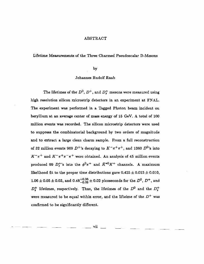
The lifetimes of the n°, v+, and Dt mesons were measured using
high resolution silicon microstrip detectors in an experiment at FNAL.
The experiment was performed in a Tagged Photon beam incident on
beryllium at an average center of mass energy of 15 GeV. A total of 100
million events was recorded. The silicon microstrip detectors were used
to suppress the combinatorial background by two orders of magnitude
and to extract a large clean charm sample. From a full reconstruction
of 32 million events 969 n+'s decaying to K-1r+1r+, and 1360 n°'s into
K-1r+ and K-7r+7r-7r+ were obtained. An analysis of 45 million events
produced 99 Dt" 's into the </>o7r+ and k*° K+ channels. A maximum
likelihood fit to the proper time distributions gave 0.435 ± 0.015 ± 0.010,
1.06 ± 0.05 ± 0.03, and 0.48!8:8~ ± 0.02 picoseconds for the n°' n+' and
nt lifetimes, respectively. Thus, the lifetimes of the no and the Dt were measured to be equal within error, and the lifteime of then+ was
confirmed to be significantly different.
vii
1
1.1 1.1.1 1.1.2 1.2 1.3 1.4
2
2.1 2.2
3
3.1 3.2 3.3 3.4 3.5 3.6 3.6.1 3.6.2 3.6.3 3.7
Contents
List of Figures List of Tables
Perspectives
On Charm· On Charm States On Charm Decay and Lifetime On Charm Production and Detection On Photo-production of Charm On Experiment E691
The Beam •••
The Photon Beam The Tagging System
The Spectrometer
The Target The Silicon Microstrip Detectors The Magnets The Drift Chambers The Cerenkov Counters The Calorimeters The Electromagnetic Shower Calorimeter The Hadron Calorimeter The Pairplane The Muon Walls
viii
page
x xiii
1
2 2 3
16 18 20
22
22 26
31
33 35 41 42 49 55 56 60 63 64
4
4.1 4.1.1 4.1.2 4.1.3 4.2 4.3
5
5.1 5.2
6
6.1 6.2
'T
7.1 7.2 7.3
8
The Data Collection
The Triggers The Physics Triggers The Calibration Triggers The Test Triggers The Data Acquisition The Monitor
The Reconstruction
Passl Pass2
Data Analysis
The Data Reduction The Final Event Selection
The Lifetime Analysis
The Lifetime Fit The Monte Carlo The Corrections and the Error Analysis
Synopsis •
Appendix
References
ix
69
69 70 75 77 78 80
84
84 88
94
94 102
111
111 117 118
126
132
139
List of Figures
Figure page
1.1 The SU(4) meson multiplets 4 1.2 The SU( 4) baryon multiplets 4 1.3 Semi-leptonic charm decay diagrams 5 1.4 Hadronic charm decay diagrams 6 1.5 Lowest order decay diagrams for charmed mesons 9 1.6 Quark graphs exhibiting the operator structure of the QCD 11
renormalized Lagrangian 1.7 Interfering graphs for the D+ 12 1.8 Absence of interference in D0 and Dt decays 12 1.9 Final state interactions in v0 -+<PK 13 1.10 Schematic of a production (primary) and decay (secondary) 18
vertex 1.11 Charm hadro-production via quark annihilation and gluon 19
scattering. 1.12 First order graph for photon gluon fusion 19 1.13 Second order diagrams to photon gluon fusion 20
2.1 Layout of Fermilab: the accelerator and the beamlines 23 2.2 The electron yield per incident proton 24 2.3 Schematic of the beamline 25 2.4 A schematic of the electron detection system 26 2.5 Schematic of the shower counters in the Tagging System 28 2.6 The E691 photon spectrum 29 2.7 The ratio of tagged to reconstructed energy in J / 't/J decays. 30
3.1 The E691 version of the Tagged Photon Spectrometer 32 3.2 The target and the nine microstrip planes 35 3.3 A cross section of a microstrip plane 36 3.4 A small microstrip plane and the printed circuit fan-out 37 3.5 The target and the vert"ex detector as seen by an incident 40
photon 3.6 Cut away view of a drift chamber station 45 3.7 Cell structure of a drift chamber triplet 45
x
3.8 Real and perfect t-zero distribution 49 3.9 Cerenkov light intensities versus momentum 51 3.10 The upstream Cerenkov counter: Cl 53 3.11 The Cl optics and mirror segmentation 53 3.12 The downstream Cerenkov counter: C2 54 3.13 The C2 optics and mirror segmentation 54 3.14 Cutaway view of the SLIC 59 3.15 SLIC interior and the corrugated panels 59 3.16 The Hadrometer 61 3.17 The Pairplane 63 3.18 The Front Muon Wall 65 3.19 The Back Muon Wall 66
4.1 Schematic of the TAGH trigger and ET gate 70 4.2 ET distribution for hadronic events in TAGH data 72 4.3 ET distribution for charm events in TAGH data 72 4.4 Schematic of the ET trigger 73 4.5 Charm enhancement as a function of ET 74 4.6 The Dimuon trigger logic 76 4.7 The PDP-11 databus configuration 80 4.8 The On-Line Monitor structure 81
5.1 The tracking regions and the coordinate systems 86 5.2 Reconstructed particles in the SLIC 90 5.3 Cerenkov probabilities for pions 91 5.4 Cerenkov probabilities for kaons 91 5.5 An event with reconstructed charm vertices 93
6.1 K 1r invariant mass distribution without vertex cuts 96 6.2 Transverse miss distance (DIP) in candidate n° -+ K1r 97
events 6.3 K1r invariant mass distributions for different SDZ cuts 99 6.4 Signals for the n° lifetime analysis 105 6.5 Signals for the n+ lifetime analysis 106 6.6 Signals for the nt lifetime analysis 107 6.7 Time distribution for the Do 108 6.8 Time distribution for then+ 109 6.9 Time distribution for the D"t 110
7.1 Background subtracted proper time distributions for n° 114 7.2 Background subtracted proper time distribution for v+ 115 7.3 Background subtracted proper time distributions for Dt 116 7.4 Comparison of Monte Carlo distributions with data 119
xi
7.5
7.6
A.1 A.2 A.3 A.4 A.5
The difference between the generated Monte Carlo and reconstructed time. Background subtracted proper time distribution for n+, with strict fiducial cut
Schematic of a decay in the target A typical primary vertex distribution for n+ A "Y-distribution for n+ The gain in acceptance versus decay position The ti-distribution for then+
xii
122
124
133 133 135 136 138
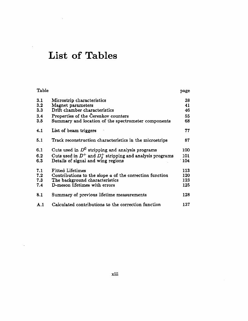
List of Tables
Table page
3.1 Microstrip characteristics 38 3.2 Magnet parameters 41 3.3 Drift chamber characteristics 46 3.4 Properties of the Cerenkov counters 55 3.5 Summary and location of the spectrometer components 68
4.1 List of beam triggers 77
5.1 Track reconstruction characteristics in the microstrips 87
6.1 Cuts used in n° stripping and analysis programs 100 6.2 Cuts used inn+ and Dt stripping and analysis programs 101 6.3 Details of signal and wing regions · 104
7.1 Fitted Lifetimes 113 7.2 Contributions to the slope a of the correction function 120 7.3 The background characteristics 123 7.4 D-meson lifetimes with errors 125
8.1 Summary of previous lifetime measurements 128
A.1 Calculated contributions to the correction function 137
xiii

1
1 Perspectives
Precise measurements of branching ratios and lifetimes have in-
duced major changes in charm physics. A wide range of theoretical ideas
has been used to explain the data. It has been necessary to bring to
gether the weak and the strong interactions even though they are dom-
inant on completely different distance scales. On the experimental side,
the arena of charm has seen a shift of focus from colliding beam exper-
iments at SLAC and DESY to a new generation of fixed target experi-
ments at FNAL. Early results from the first of these experiments, E691,
are presented in this thesis. We report on the first high statistics lifetime
measurements of the three pseudoscalar charmed mesons, the D0 , v+ and
ntt.
This chapter contains a very brief review of some important as-
pects of charm, theoretical as well as experimental. Particular emphasis
is placed on charm decays and lifetimes. In the succeeding chapter the
generation of the E691 photon beam is described. A general description of
the spectrometer and its detector components follows. Chapter 4 covers
t Traditionally the F+. We shall be progressive and continue to use the 1986 Particle Data Group nomenclature.
2
the on-line systems: the triggers, the data acquisition and the monitor.
The event reconstruction is discussed in chapter 5. Next comes a section
on data analysis and signal extraction which is followed by a discussion of
the lifetime analysis. Some detailed calculations pertaining to the lifetime
systematics are given in the appendix. The thesis concludes with a short
summary and a look to the future.
1.1 On Charm
The first proposal for a fourth quark, charm, was made in 1964 for
purely esthetic reasons-to preserve the equality between the number of
quarks and leptons. Since there was no physical need for the additional
quark it was soon forgotten. In 1972 the '4-quark' idea was reintroduced
via the GIM mechanism to explain the suppression of strangeness chang
ing neutral currents and the KL-Ks mass difference. The charmed quark
was quickly assimilated into the group theoretical structure of the 'quark
model'. In their classic review Gaillard, Lee and Rosner [Ga75] described
the expected structure and hierarchy of charmed baryons and mesons. Be
fore the first charmed particle was observed, they estimated the charmed
quark mass and predicted its lifetimes.
1.1.1 On Charm States
The puzzle of the organization of hadronic matter was solved in the
late 1950's. The solution, known as the Eightfold- Way or SU(3) flavour
symmetry, explained why there were heavy and light particles, baryons
3
and mesons, and why some of the particles shared certain properties but
not others.
At that time only three types-flavours-of quarks were known:
up, down and strange {u,d,s). However, the general prescription for
making hadrons is the same for any number of flavours: baryons are made
from three quarks-qqq, and mesons from a quark and anti-quark-qq. By
taking all possible qq and spin combinations one obtains, for three quarks,
nine spin-0 and nine spin-1 mesons. In the four quark scheme one finds
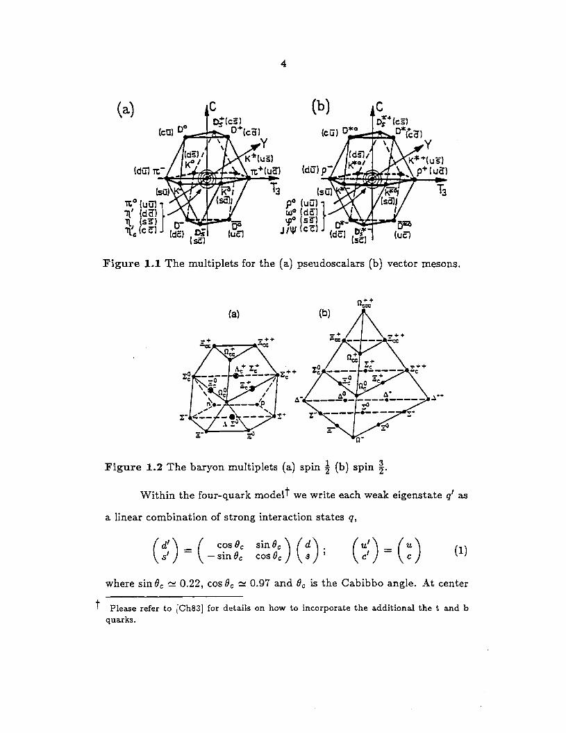
sixteen mesons of each spin. Figures 1.1 and 1.2 show the quark structure
of the groundstate meson and baryon multiplets.
All the pseudoscalar and vector charmed mesons have been ob
served. Knowledge of the Dt and Dt* is sparse, but finally reliable data
is accumulating, especially for the Dt. Of the baryons only the single
charmed spin i particles have been reported. And of those, only the Ac
has data-marginal at that-on branching ratios and lifetime.
1.1.2 On Charm Decay and Lifetime
The charmed quark decays into a strange quark and a lepton
antineutrino or an ud quark-antiquark pair. The process is described
by the standard weak interaction model. However, there is a small com
plication: the 'weak' quarks produced in the charm decay are slightly
different from the 'strong' quarks which are bound into hadrons that we
can observe.
4
(a) (b) c o: .. {cs)
-.::::~ .. ~{~Cf) y
Figure 1.1 The multiplets for the (a) pseudoscalars (b) vector mesons.
~··
Figure 1.2 The baryon multiplets (a) spin! (b) spin !· Within the four-quark modelt we write each weak eigenstate q' as
a linear combination of strong interaction states q,
( d
1) ( cos Be
s1 = - sinOe sin Be) ( d) . cos Be s ' (~:)-(~) (1)
where sin Oe ~ 0.22, cos Oc ~ 0.97 and Be is the Cabibbo angle. At center
t Please refer to [Ch83] for details on how to incorporate the additional the t and b quarks.
5
of mass energies well below the W boson mass of 82 Ge V, the term in the
weak Lagrangian that reduces the charm quantum number of the initial
state by one unit is
.Cac=l = ~(SL/µCLCOSIJc - ~/µCLsinOc) x
(oe/µeL + Oµ/µµ,L + Or/µTL+
a L/µdL cos Oc +a LIµ s L sin Oc), (2)
with u, d, s, c representing the field operators for the quarks, e, µ,, r and
lie, llµ, llr for the leptons and neutrinos. The subscript L indicates that
only the left-handed component tPL = !(1+1s)t/J of the particle partici-
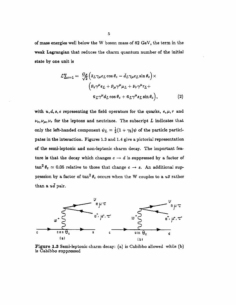
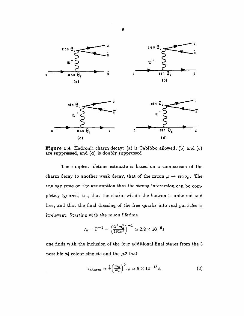
pates in the interaction. Figures 1.3 and 1.4 give a pictorial representation
of the semi-leptonic and non-leptonic charm decay. The important fea-
ture is that the decay which changes c -+ d is suppressed by a factor of
tan2 6c ~ 0.05 relative to those that change c -+ s. An additional sup
pz:ession by a factor of tan2 Oc occurs when the W couples to a us rather
than a ud pair.
+ . . e ' }1'" ' i:: ...
c c Cal
sin 9c
( b)
+ . e 'y,i:-...
d
Figure 1.3 Semi-leptonic charm decay: (a) is Cabibbo allowed while (b) is Cabibbo suppressed
6
u u
-d
d
c s c d
u
$ s
c c d
Figure 1.4 Hadronic charm decay: (a) is Cabibbo allowed, (b) and (c) are suppressed, and ( d) is doubly suppressed
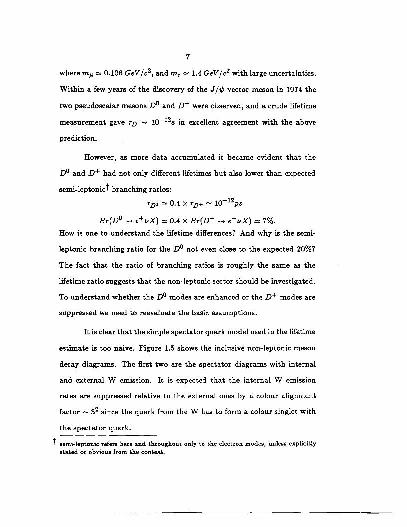
The simplest lifetime estimate is based on a comparison of the
charm decay to another weak decay, that of the muon µ, --+- eiJeLIµ.- The
analogy rests on the assumption that the strong interaction can be com-
pletely ignored, i.e., that the charm within the hadron is unbound and
free, and that the final dressing of the free quarks into real particles is
irrelevant. Starting with the muon lifetime
-1 (G2ms )-1 -6 Tµ = r = ~ ~ 2.2 X 10 S
one finds with the inclusion of the four additional final states from the 3
possible qq colour singlets and the µv that
T .._ 1 ( mµ) 5 r .._ 8 X 10-13 ,.. charm '- 5 me µ - ~, (3)
7
where mµ ~ 0.106 GeV/c2, and me~ 1.4 GeV/c2 with large uncertainties.
Within a few years of the discovery of the J /t/; vector meson in 1974 the
two pseudoscalar mesons D0 and v+ were observed, and a crude lifetime
measurement gave TD - 10-12 s in excellent agreement with the above
prediction.
However, as more data accumulated it became evident that the
D0 and v+ had not only different lifetimes but also lower than expected
semi-leptonic t branching ratios:
rDo ~ 0.4 x TD+ ~ 10-12ps
Br(D0 ~ e+vx) ~ 0.4 x Br(D+ ~ e+vx) ~ 7%.
How is one to understand the lifetime differences? And why is the semi-
leptonic branching ratio for the D0 not even close to the expected 20%?
The fact that the ratio of branching ratios is roughly the same as the
lifetime ratio suggests that the non-leptonic sector should be investigated.
To understand whether the n° modes are enhanced or the n+ modes are
suppressed we need to reevaluate the basic assumptions.
It is clear that the simple spectator quark model used in the lifetime
estimate is too naive. Figure 1.5 shows the inclusive non-leptonic meson
decay diagrams. The first two are the spectator diagrams with internal
and external W emission. It is expected that the internal W emission
rates are suppressed relative to the external ones by a colour alignment
factor - 32 since the quark from the W has to form a colour singlet with
the spectator quark.
t semi-leptonic refers here and throughout only to the electron modes, unless explicitly stated or obvious from the context.
8
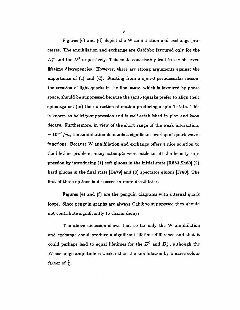
Figures (c) and (d) depict ·the W annihilation and exchange pro
cesses. The annihilation and exchange are Cabibbo favoured only for the
Dl and the Do respectively. This could conceivably lead to the observed
lifetime discrepencies. However, there are strong arguments against the
imp~rtance of (c) and (d). Starting from a spin-0 pseudoscalar meson,
the creation of light quarks in the final state, which is favoured by phase
space, should be suppressed because the (anti-)quarks prefer to align their
spins against (in) their direction of motion producing a spin-1 state. This
is known as helicity-suppression and is well established in pion and kaon
decays. Furthermore, in view of the short range of the weak interaction,
- 10-3 fm, the annihilation demands a significant overlap of quark wave
functions. Because W annihilation and exchange offers a nice solution to
the lifetime problem, many attempts were made to lift the helicity sup
pression by introducing (1) soft gluons in the initial state [Rii83,Sh80] (2)
hard gluons in the final state [Ba79] and (3) spectator gluons [Fr80]. The
first of these options is discussed in more detail later.
Figures (e) and (f) are the penguin diagrams with internal quark
loops. Since penguin graphs are always Cabibbo suppressed they should
not contribute significantly to charm decays.
The above dicussion shows that so far only the W annihilation
and exchange could produce a significant lifetime difference and that it
could perhaps lead to equal lifetimes for the n° and nt, although the
W exchange amplitude is weaker than the annihilation by a naive colour
factor of i·
9
(a) (b) (c)
l>< ( f)
Figure 1.5 Lowest order decay diagrams for charmed mesons: (a) spectator external W emission, (b) spectator internal W-emission, ( c) Wexchange, (d) W-annihilation, (e) penguin, (f) sideways penguin.
In the compariSon of charm to muon decay the strong interactions
were neglected. In a first attempt to include QCD one rewrites Eq. (2),
keeping only the non-leptonic and Cabibbo favoured terms, as
.C:Kc=l =Tz cos2 Be( c-0- + c+O+)
20- =(sc)(ud) - (uc)(sd)
20+ =(sc)(ud) + (uc)(sd),
(4)
(Sa)
(5b)
where the 'left-handed' subscript is suppressed, and o_ and O+ have
definite SU(3)colour transformations. They transform as a 6 and a 151,
respectively. The operators also form a 20- and 84-plet under SU( 4j f ro-
tations. The constants C- and c+ are the renormalized Wilson coefficients
which are both equal to unity in the absence of strong interactions and
satisfy C-C~ = 1. Because of the distinct SU(3)c symmetry properties of
0+ ( 0-), the renormalization of the four-fermion vertex leads to a repul
sive (attractive) hard gluon exchange. Thus the values of c± change from
10
one to [ Ge84,R ii83]
C- ~ 1.5, c+ ~ 0.8.
There is some leeway in these values because of the uncertainty in AQc D
and the mass scale in the renormalization. But it is always true that C- >
c+ which is known as SU(4) I 20- or SU(3)c 6-dominance. Rearrangment
of Eq. (4) leads to
.CA.c=l =~ cos2 8c ( c1(sc)(ud) + c2(uc)(sd))
c1 =!(c+ + c-); c2 = !(c+ - c-).
(6)
(7)
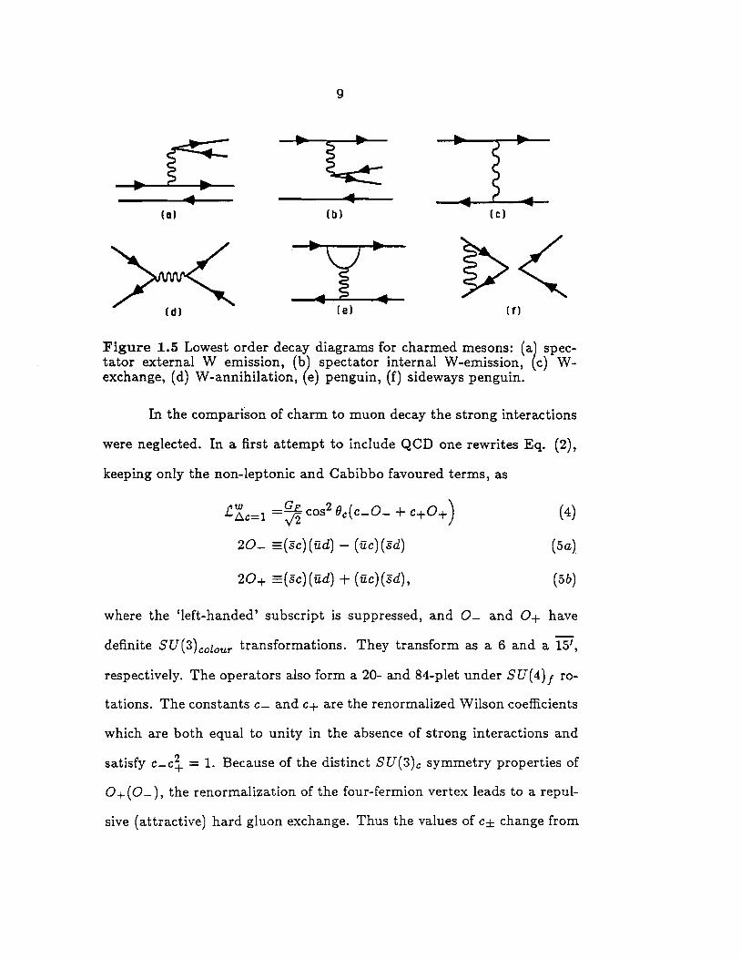
When the strong interactions are turned off c2 = 0 and thus the second
term in Eq. (6) drops away. One can understand Eq. (6) qualitatively
as a mathematical formulation of diagrams 1.6. The first term changes
c---+- sand has charge changing currents while the second term is made up
of neutral currents since c ---+- u. The second term, corresonding to graph
(b) is reduced relative to (a) by some factor that depends on the exact
values of c±. One should note that even though figures I.Sb and 1.6b are
alike they have completely different origins. In 1.Sb the colour suppression
is a non-spectator effect, while the renormalization which produces l.6b
is purely within the spectator framework and independent of the other
quark.
The vertex renormalization increases the importance of the non
leptonic over the semi-leptonic sector but does not contribute to the life
time inequality. The decrease in the semi-leptonic branching ratios from
these short distance QCD effects is estimated to be about 20-25% [Rii86],
c~~ s
(a)
11
s
(b)
Figure 1.6 Quark graphs exhibiting the operator structure of the Lagrangian of Eq. (6) (a) the c1 type (b) the c2 type.
i.e, the original ratio of 20% is now about 15% ..
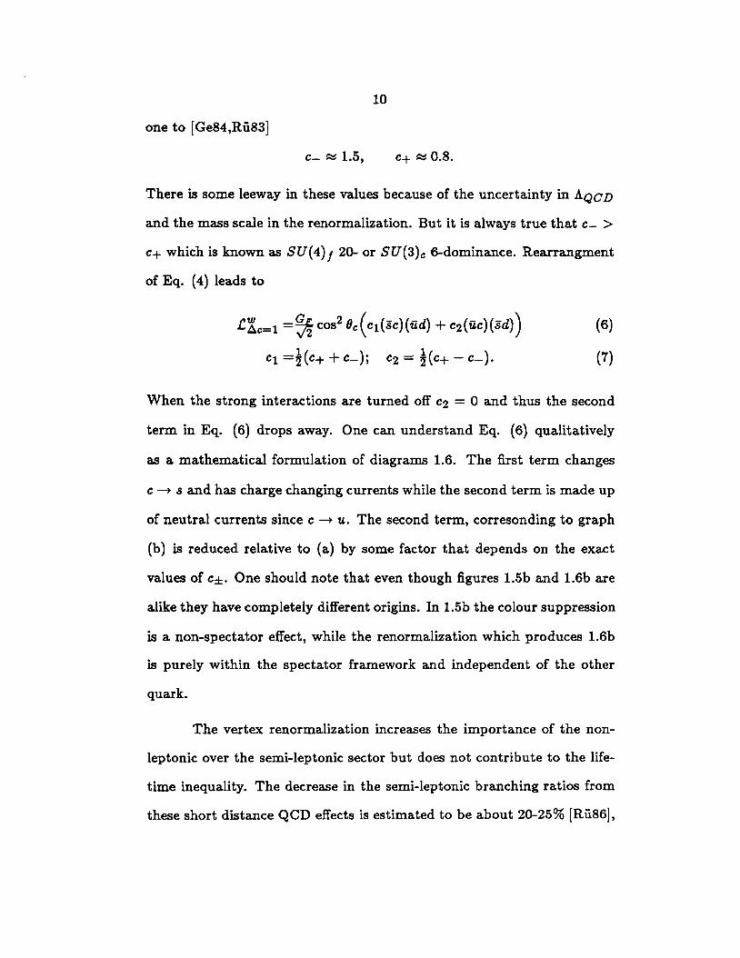
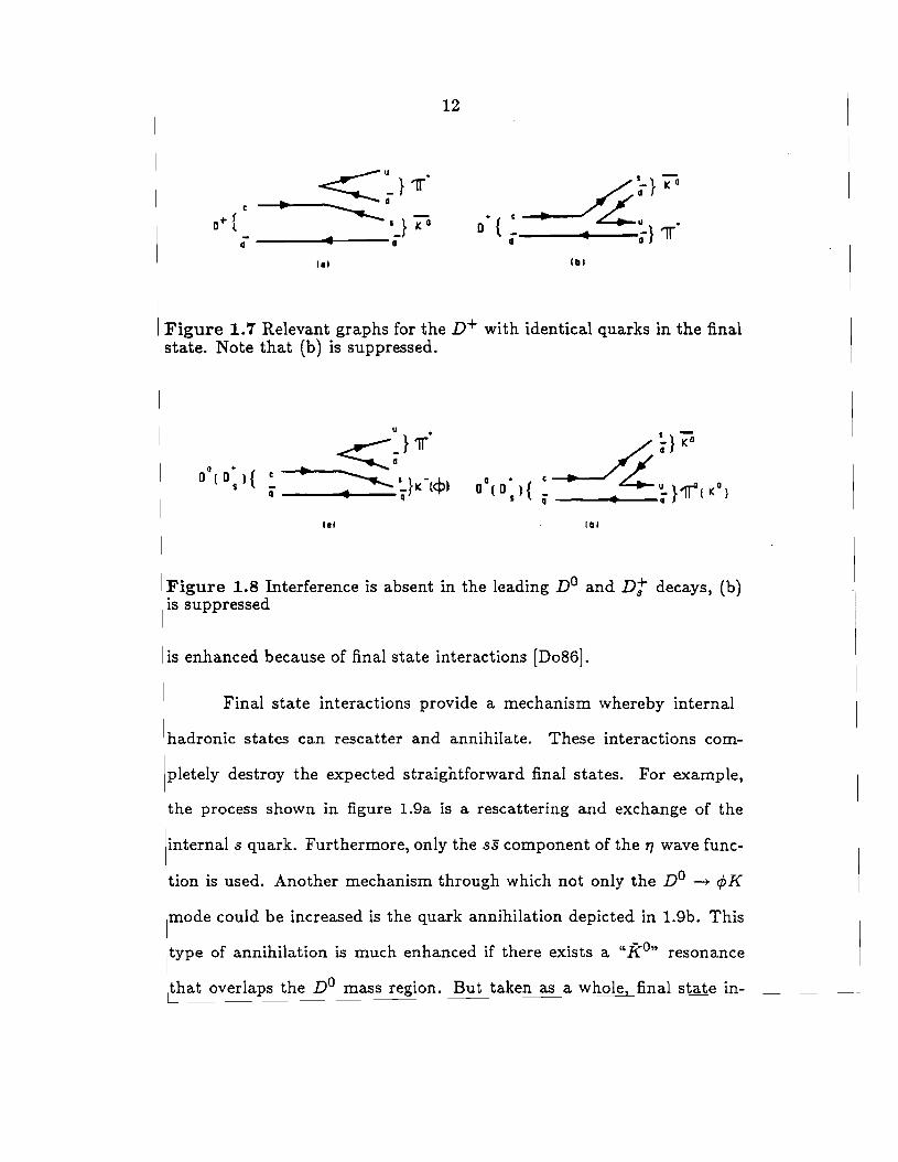
A large potential suppression of the D+ decay can be obtained
from a destructive interference in the final state [Gu79,Bi84]. Because the
D+ has two identical quarks in the end state it can form the same final
products in two different ways as illustrated in figure 1. 7. This means that
the amplitudes in Eq. (6) are added coherently, leading to a destructive
interference since c2 < 0. Figures 1.8 show that there is no such interfer
ence in the Cabibbo allowed decays of the D 0 and Dt. The interference
mechanism also explains the enhancement of the semi-leptonic branching
ratio of the D+ relative to the Do. Bag model calculations show that
the Pauli interference between the quarks alone accounts for 20-40% of
the lifetime and semi-leptonic branching ratio differences. The effect of
the interference is enhanced further, because only certain final states are
accessible to the D+ [Rii86].
Now there is substantial data on a mode that was thought to occur
only through W exchange. But the large observed rates of n° --+<PK are in
violent diagreement with that hypothesis. It is possible that this channel
<~}1( c~d
a+ { '_}Ko d d
l•l
12
1111
Figure 1. 7 Relevant graphs for the n+ with identical quarks in the final state. Note that (b) is suppressed.
lal 1111
Figure 1.8 Interference is absent in the leading n° and Dj" decays, (b) is suppressed
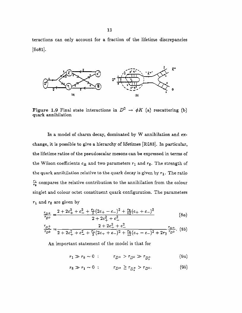
is enhanced because of final state interactions [Do86].
Final state interactions provide a mechanism whereby internal
hadronic states can rescatter and annihilate. These interactions com-
pletely destroy the expected straightforward final states. For example,
the process shown in figure 1.9a is a rescattering and exchange of the
internals quark. Furthermore, only the ss component of the TJ wave func
tion is used. Another mechanism through which not only the n° -+ ¢K
mode could be increased is the quark annihilation depicted in 1.9b. This
type of annihilation is much enhanced if there exists a "Ko" resonance
\that overlaps the n° mass region. But taken as a whole, final state in-
13
teractions can only account for a fraction of the lifetime discrepancies
(So81].
~ K s s K
~ s i
- ' u s
(a, (b)
Figure 1.9 Final state interactions in n° ~ <PK (a) rescattering (b) quark annihilation
In a model of charm decay, dominated by W annihilation and ex
change, it is possible to give a hierarchy of lifetimes [Rii.83]. In particular,
the lifetime ratios of the pseudoscalar mesons can be expressed in terms of
the Wilson coefficients c± and two parameters ri and rs. The strength of
the quark annihilation relative to the quark decay is given by r 1. The rati.o
~ compares the relative contribution to the annihilation from the colour
singlet and colour octet constituent quark configuration. The parameters
r1 and rs are given by
An important statement of the model is that for
(Ba)
(9a)
(9b)
14
The explanation of these relations is that for the singlet dominance the
W annihilation into leptons is very important for the Dt, while for octet
dominance, case (b), the annihilation is colour suppressed.
The W annihilation model can be tested by precise measurements
of lifetimes, and/or nt semi-leptonic branching ratios or by the observa
tion of non-leptonic annihilation amplitude that can not be questioned by
final state interaction magic.
An integration of all the previously discussed effects seems to have
been achieved by Bauer, Stech, and Wirbel [Ba85,Ba86b]. Their calcu-
lational approach rests on a factorization scheme in which they 'form'
hadrons from the quark currents rather than dealing with short and long
distance effects at the quark level. They consider the transition amplitude
A
A(D-+ I) ex ai (fl(8"'Yµc)H(ii"'Yµd)HID)+
a2 (II (fl"'Yµc)H (8"'Yµd)HID) (11)
(12)
where f denotes a two body final state of pseudoscalar and/or vector
mesons and e is a colour alignment factor which accounts for colour mis-
matches due to quark mass effects, internal W emission etc .. It is expected
that e ~ N 1 = -31 but it is left as an undetermined parameter. The
colour
authors computed a large number of partial widths in terms of ai and a2.
A fit to the 1985 MARKIII data gave
a2 ~ -0.55.
15
We see that a2 < 0 and that therefore interference is present. In addi-
tion, when final state interactions were included in their calculations the
agreement with the data improved significantly.
The factorization ansatz has found confirmation in a it; expan
sion where it; is the number of colours [Bu86]. The matrix elements are
expanded according to
and only the lowest order term ~ is retained. It is found that the colour
alignment factor e as defined by Eq. (12) is small, perhaps zero, and
should be neglected, especially in view_ of keeping only the lowest order
in -ft;. Neglecting phase space factors and QCD radiative corrections the
authors find that
TDO 2c1 C2 + e( CI + c~) -- ,...., 1 + r--------rn+ - i + ci + c~ + ec1 c2.
(13)
The parameter r measures the effectiveness of the interference and can
have values between zero and one. It is commonly taken to be about 0. 7.
From the preceeding discussion we see that information on the size
of W annihilation/exchange, final state interactions and the effectiveness
of the interference is needed. More data on branching ratios is useful in
sorting through the effects of final state interactions and the interference.
In particular, a good lifetime measurement of the Di could determine
whether the Di behaves like the Do, the n+, or neither.
16
1.2 On Charm Production and Detection
Early charm experiments at fixed target accelerators were not very
successful because of poor signal-to-noise ratios. In contrast, electron-
positron colliding beam experiments dominated the field because a large
fraction of the events contained charm.
In electron-positron collisions the hadronic production cross section
is approximately
u(e+ e- --+ qlj =hadrons) """ 4j~2
. E Q~, q=u,d,s,c
(14)
where Qq is the charge of the quark, .s the center of mass energy squared
and a the fine structure constant. From this one obtains that above
threshold 40% of all hadronic final states contain charm. Significant back-
ground reductions are achieved by constraining the event energy to the
beam energy. Moreover, at y'8 = 3. 768 Ge V a t/J resonance, the ,,P11,
decays exclusively into n° D0 and n+ n- mesons. Unfortunately, deter-
mining lifetimes at such low energies is impossible because the mesons are
produced essentially at rest and thus decay near the production point.
The average charged track multiplicities in e+ e- charm experi-
ments is - 4.4/event [Hi85] as compared to about 10/event in photo- and
hadro-production. Thus, the combinatorial background is much larger.
Nevertheless, fixed target experiments are useful because of their potential
for direct lifetime measurements and their high luminosities. In addition,
it is possible to observe the entire charm mass spectrum without changing
the beam energy. And finally, with the development of silicon microstrip
17
detectors at CERN by NAll/32 [He81,Ri86] the background rejection in
charm events has increased by two orders of magnitude. The high resolu-
tion of these detectors allows a clean separation of the long lived charm
from the non-charm backgrounds.
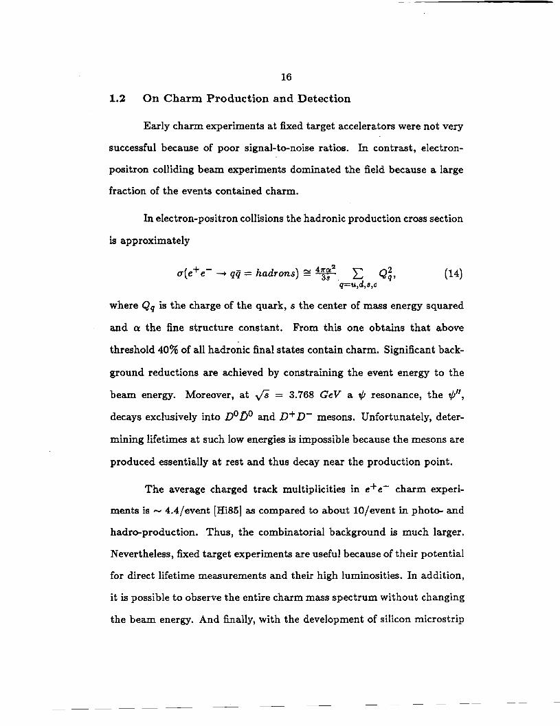
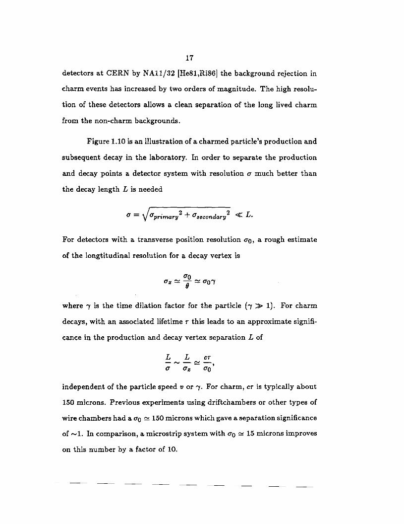
Figure 1.10 is an illustration of a charmed particle's production and
subsequent decay in the laboratory. In order to separate the production
and decay points a detector system with resolution a much better than
the decay length L is needed
For detectors with a transverse position resolution ao, a rough estimate
of the longtitudinal resolution for a decay vertex is
where I is the time dilation factor for the particle (I > 1). For charm
decays, with an associated lifetime r this leads to an approximate signifi-
cance in the production and decay vertex separation L of
L L CT ------ ' a az ao
independent of the particle speed v or 'Y • For charm, er is typically about
150 microns. Previous experiments using driftchambers or other types of
wire chambers had a uo ~ 150 microns which gave a separation significance
of -1. In comparison, a microstrip system with uo ~ 15 microns improves
on this number by a factor of 10.
18
primary 4-----6Z -----4•~
Figure 1.10 Schematic of a production (primary) and decay (secondary) vertex.
The combinatorics in candidate charm events is dramatically re-
duced when the separation significance is used as a criterion for a probably
charm content. It is very unlikely for random tracks to form a false vertex
with small errors.
1.3 On Photo-production of Charm
In charm production photon beams have an considerable advan-
tage over proton, pion, and kaon beams. At comparable center of mass
energies, the fractional charm content of the total hadronic cross section
is 5-10 times larger in photo-production than in hadro-production. Thus,
the backgrounds are lower when photons are used to create charm.
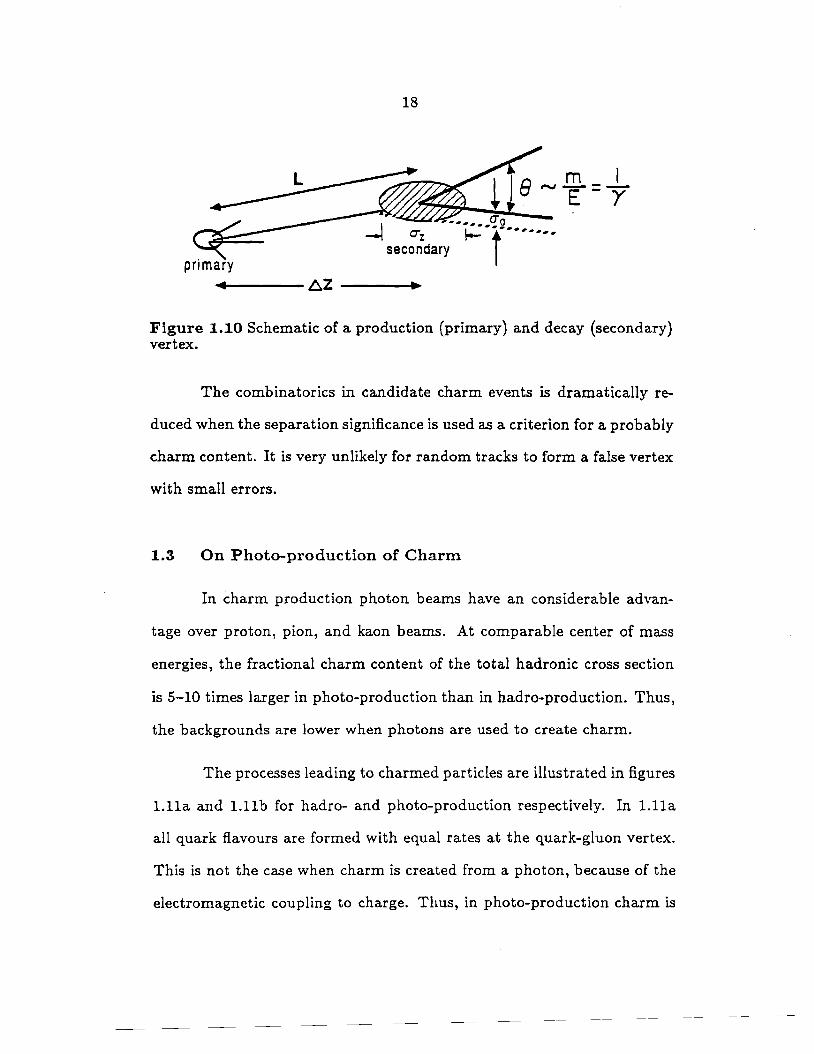
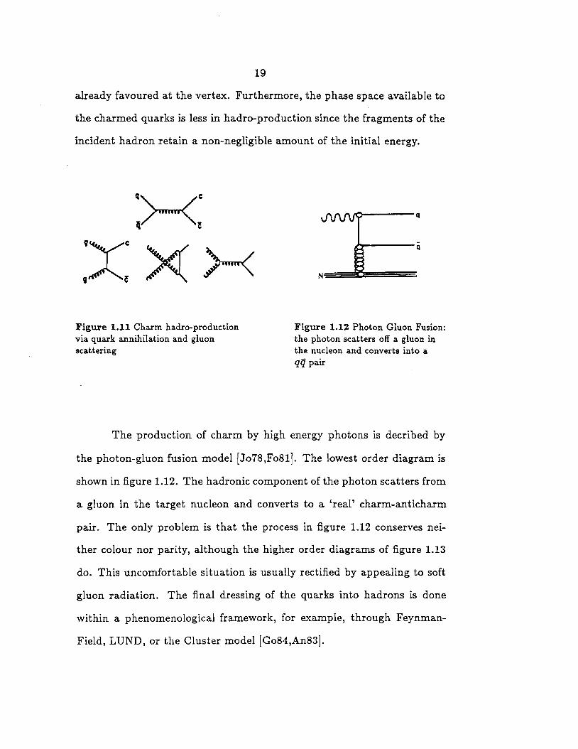
The processes leading to charmed particles are illustrated in figures
1.lla and 1.llb for hadro- and photo-production respectively. In 1.lla
all quark flavours are formed with equal rates at the quark-gluon vertex.
This is not the case when charm is created from a photon, because of the
electromagnetic coupling to charge. Thus, in photo-production charm is
19
already favoured at the vertex. Furthermore, the phase space available to
the charmed quarks is less in hadro-production since the fragments of the
incident hadron retain a non-negligible amount of the initial energy.
:x: )<( >-< Figure 1.11 Charm hadro-production via quark annihilation and gluon scattering
Figure 1.12 Photon Gluon Fusion: the photon scatters off a gluon in the nucleon and converts into a qij pair
The production of charm by high energy photons is decribed by
the photon-gluon fusion model [Jo78,Fo81]. The lowest order diagram is
shown in figure 1.12. The hadronic component of the photon scatters from
a gluon in the target nucleon and converts to a 'real' charm-anticharm
pair. The only problem is that the process in figure 1.12 conserves nei-
ther colour nor parity, although the higher order diagrams of figure 1.13
do. This uncomfortable situation is usually rectified by appealing to soft
gluon radiation. The final dressing of the quarks into hadrons is done
within a phenomenological framework, for example, through Feynman-
Field, LUND, or the Cluster model [Go84,An83].
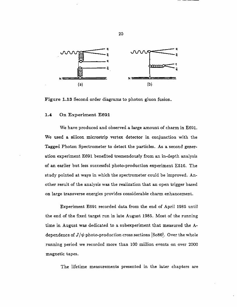
20
q q
q ij
q q
q q
N
(a) (b)
Figure 1.13 Second order diagrams to photon gluon fusion.
1.4 On Experiment E691
We have produced and observed a large amount of charm in E691.
We used a silicon microstrip vertex detector in conjunction with the
Tagged Photon Spectrometer to detect the particles. As a second gener-
ation experiment E691 benefited tremendously from an in-depth analysis
of an earlier but less successful photo-production experiment E516. The
study pointed at ways in which the spectrometer could be improved. An-
other result of the analysis was the realization that an open trigger based
on large transverse energies provides considerable charm enhancement.
Experiment E691 recorded data from the end of April 1985 until
the end of the fixed target run in late August 1985. Most of the running
time in August was dedicated to a subexperiment that measured the A
dependence of J /1/l photo-production cross sections [8086]. Over the whole
running period we recorded more than 100 million events on over 2000
magnetic tapes.
The lifetime measurements presented in the later chapters are

21 I
based on an analysis of 32 million events for about one thousand n°
and n+ signal events each, and an analysis of 45 million events for one
!hundred Dt. Considering that this amount of data is already more than
the total of all previous lifetime experiments we believe that E691, and in
general silicon microstrip detectors, have brought a revolution to charm
physics.
22
2 The Beam
Our experiment at the Tagged Photon Lab benefited from several
major changes to the accelerator. Because of the increased proton energy
available at the Tevatron, 800 rather than 400 Ge V, we extended the
incident photon energy spectrum from 170 to 260 Ge V; charm production
cross sections increase noticably with energy. We were also able to take
full advantage of the new long spill cycle. With the 20-fold increase in
spill length we recorded many more events which otherwise would have
been lost to system dead-time.
2.1 The Photon Beam
The photon beam was the result of a four step process initiated by
protons. The main intermediate particles were electrons. At the entrance
to the experimental hall the electrons were induced to radiate photons for
the experiment.
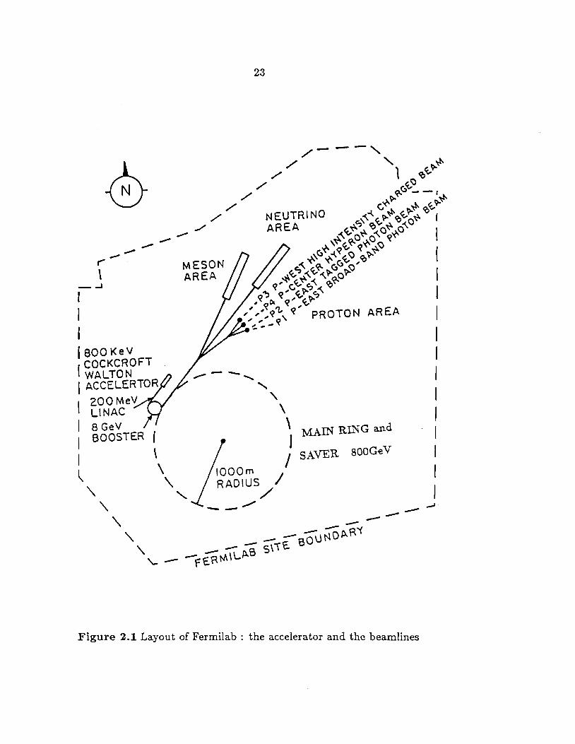
Every minute, more than 1013 protons were extracted from the
Tevatron over a 22 second interval. About one fifth of those protons were
designated for the Tagged Photon Beam (see figure 2.1). The protons
interacted in a 30 cm beryllium target and produced high energy secon-
( 800 KeV
ICOCKCROFT WALTON
I ACCELERTOR
I 200MeV UNAC
I 8 GeV I BOOSTER
I ~ '\
l \ \ \
'
23
' ' \
lOOOm RADIUS I
/
\ 1
I
MAIN RING and
SAVER sooGeV
' __ ,,,,. __ _,. --'\ -- --' -- -- OuN'O~R"< '\ -- -- ;6 5\\€. e
'- -- --f€,RM\L
Figure 2.1 Layout of Fermilab : the accelerator and the beamlines
24
daries. The ensuing charged particles were swept aside by magnets into
beam dumps. The surviving neutral beam, consisting mainly of kaons,
neutrons, and photons from neutral pion decay, passed through a radiator
to convert the photons to electron-positron pairs. The electrons were se-
lected, collimated and sent down the beamline toward TPL while the other
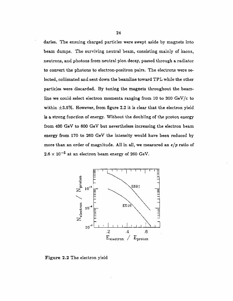
particles were discarded. By tuning the magnets throughout the beam-
line we could select electron momenta ranging from 10 to 300 Ge V / c to
within ±3.5%. However, from figure 2.2 it is clear that the electron yield
is a strong function of energy. Without the doubling of the proton energy
from 400 Ge V to 800 Ge V but nevertheless increasing the electron beam
energy from 170 to 260 Ge V the intensity would have been reduced by
more than an order of magnitude. All in all, we measured an e / p ratio of
2.6 x 10⁻⁵ at an electron beam energy of 260 Ge V.
c 0 s.. ..., CJ
~ QJ
z
.2 .4 .6
Eeleclron / Eprolon
Figure 2.2 The electron yield
25
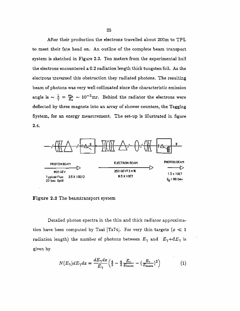
After their production the electrons travelled about 200m to TPL
to meet their fate head on. An outline of the complete beam transport
system is sketched in Figure 2.3. Ten meters from the experimental hall
the electrons encountered a 0.2 radiation length thick tungsten foil. As the
electrons traversed this obstruction they radiated photons. The resulting
beam of photons was very well collimated since the characteristic emission
angle is ,....; ~ = T, ,....; 10-3mr. Behind the radiator the electrons were
deflected by three magnets into an array of shower counters, the Tagging
System, for an energy measurement. The set-up is illustrated in figure
2.4.
PROTON BEAN ELECTRON BEAM PHOTON BEAN
l> 250 GEVt 3. '1 "
l> t> 800GEV
1.3 x IOE7 Typical Flux 2.5 X 10El2 6.SX IOE7 22 Sec. Spi11 E~ > 80 Gev
Figure 2.3 The beamtransport system
Detailed photon spectra in the thin and thick radiator approxima-
tion have been computed by Tsai [Ts74]. For very thin targets (x « 1
radiation length) the number of photons between E1 and E1 +dE1 is
given by
( ) d dE1 dx (4 4 E.., ( E.., )2) NE dE x- - - - -I I - E 3 3 Ebeam Ebeam
I (1)
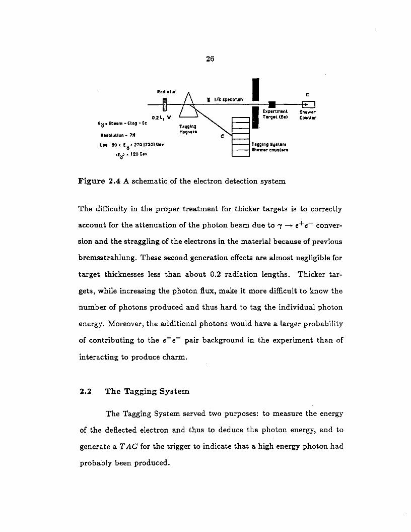
Ets = Ebeem - £tag - Ee
RHolutlon - 7:1
UH 80 < Eu ( 220 l2SOI Gav
<Eu> • 120 Gev
Tagging Magnet•
26
I Ilk spectrum I c
Torgel (Be) Counter I [>Cp1r1m1nt Shower
Tagging System Shower caunttra
Figure 2.4 A schematic of the electron detection system
The difficulty in the proper treatment for thicker targets is to correctly
account for the attenuation of the photon beam due to 'Y -+ e+ e- conver-
sion and the straggling of the electrons in the material because of previous
bremsstrahlung. These second generation effects are almost negligible for
target thicknesses less than about 0.2 radiation lengths. Thicker tar-
gets, while increasing the photon flux, make it more difficult to know the
number of photons produced and thus hard to tag the individual photon
energy. Moreover, the additional photons would have a larger probability
of contributing to the e+ e- pair background in the experiment than of
interacting to produce charm.
2.2 The Tagging System
The Tagging System served two purposes: to measure the energy
of the deflected electron and thus to deduce the photon energy, and to
generate a TAG for the trigger to indicate that a high energy photon had
probably been produced.
27
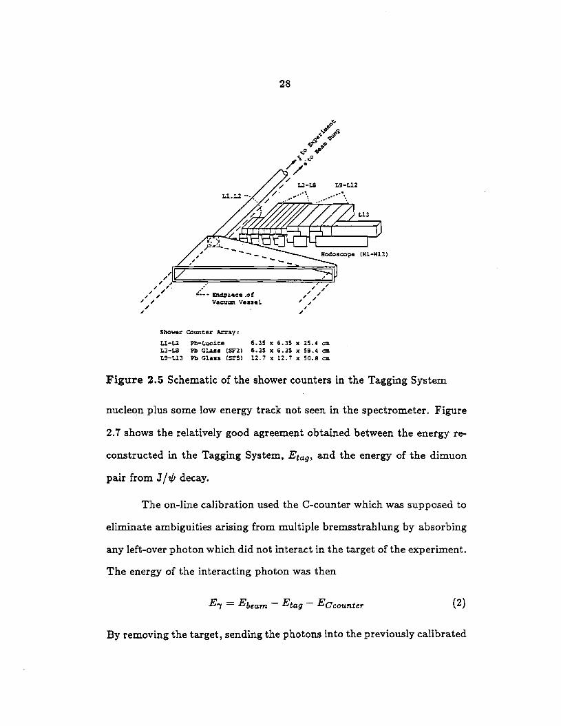
The energies and positions were measured by two lead lucite blocks,
11 and 12, and eleven lead glass blocks, 13 through 113. 11 was posi
tioned such that it barely accepted a 200 GeV electron while 113, lying
on its side, missed electrons with an energy less than about 15 GeV. RCA
6342A photomultiplier tubes measured the light output from the blocks.
The anode signals were fed to 1RS 2249 ADC's for digitization. The dyn
ode signals were discriminated and latched, and made up part of TAG.
In the early stages of the experiment additional information was
provided by hodoscope counters Hl-H13. As shown in figure 2.5 these thin
scintillation counters were layered such that an electron passed through
two H counters before showering in the lead glass. The phototube anode
and dynode signals were discriminated, the anode was latched and the
dynode contributed the second and last part to TAG.
Originally TAG was formed by the logical AND of two adjacent
H's and the corresponding 1
As the run progressed it was realized that the hodoscopes were inefficient
and not absolutely necessary. At that time it was also decided to remove
11 from TAG which shifted the accepted photon spectrum up. The final
photon spectrum is displayed in figure 2.6.
The shower counters were calibrated by two independent methods:
every six weeks on-line, and once off-line after the run by reconstructing
the elastic photon-nucleon interaction 1N ~ pX, where X is the recoiling
28
I.J-LS L9-Ll2
.::_ • Endpiece .of Vacuum Vessel
Shower Counter Array:
Ll-L2 Pb-Lucite I.J-LS Pb Glass CSF2) L9-Ll3 Pb Glass (SFS)
6.35 x 6.JS x 25.4 cm 6.JS x 6.JS x 58.4 cm 12.7 x 12.7 x so.a cm
Figure 2.5 Schematic of the shower counters in the Tagging System
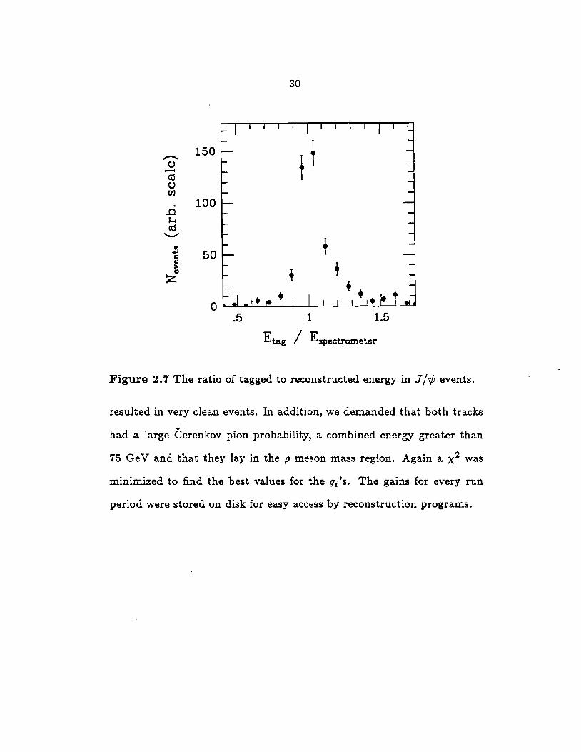
nucle~n plus some low energy track not seen in the spectrometer. Figure
2. 7 shows the relatively good agreement obtained between the energy re
constructed in the Tagging System, Etag, and the energy of the dimuon
pair from J / 't/J decay.
The on-line calibration used the C-counter which was supposed to
eliminate ambiguities arising from multiple bremsstrahlung by absorbing
any left-over photon which did not interact in the target of the experiment.
The energy of the interacting photon was then
E, = Ebeam - Etag - Eccounter (2)
By removing the target, sending the photons into the previously calibrated
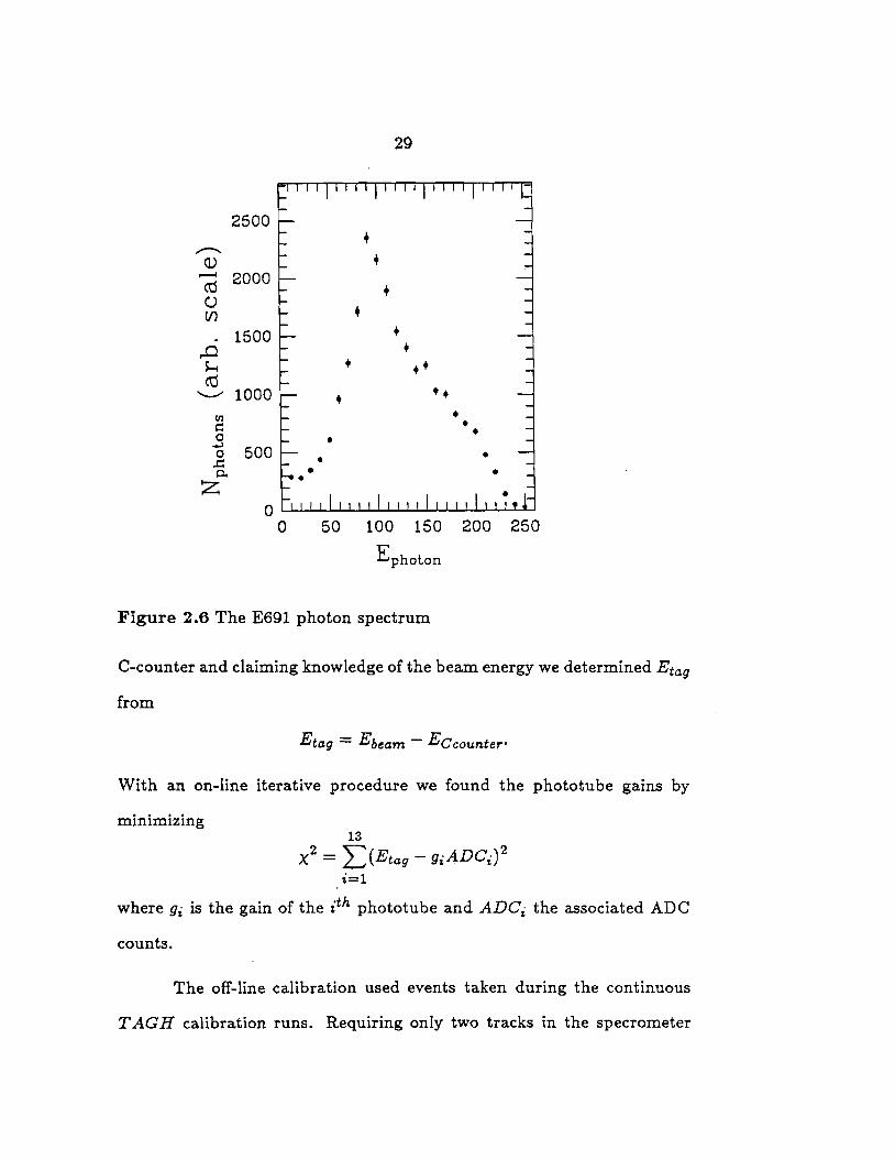
29
2500 + ,,,,,-.._,
Cl) + ......-1 2000 cO + (.)
+ (/)
1500 + . ,..0 + ~ • • • cO •• ""-" 1000 •
en • i:: • • 0 • ~ 500 0 • • ..c '1. • z
0 0 50 100 150 200 250
Ephoton
Figure 2.6 The E691 photon spectrum
C-counter and claiming knowledge of the beam energy we determined Etag
from
Etag = Ebeam - Eccounter·
With an on-line iterative procedure we found the phototube gains by
minimizing 13
x2 = L(Etag - giADCi) 2
i=l
where gi is the gain of the ith phototube and ADCi the associated ADC
counts.
The off-line calibration used events taken during the continuous
T AGH calibration runs. Requiring only two tracks in the specrometer
30
150 T t
~
Q) ....... ro 0 fl)
100 ~ s... ro
'-"'
"' + ....., 50 i::: a
+ > +
a z + + • 0 •·
.5 1 1.5
Etag / Espectrometer
Figure 2. 7 The ratio of tagged to reconstructed energy in J /1/J events.
resulted in very clean events. In addition, we demanded that both tracks
had a large Cerenkov pion probability, a combined energy greater than
75 Ge V and that they lay in the p meson mass region. Again a x2 was
minimized to find the best values for the gi 's. The gains for every run
period were stored on disk for easy access by reconstruction programs.
31
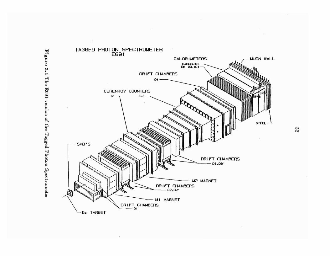
3 The Spectrometer
The Tagged Photon Spectrometer (TPS) is a conventional two
magnet spectrometer with large acceptance and good resolution. Several
major changes were made to the spectrometer since the last use of TPL by
experiment E516 [Du82,De83,Su84,Bh84]. The most significant improve
ment to the TPS was the replacement of the liquid hydrogen target-recoil
detector assembly [Ha83] by a beryllium target-silicon microstrip system
as a vertex detector [Ka85]. This exchange gained us a factor of 50 in
vertex resolution! For E691 we were able to raise the overall tracking ef
ficiency from 80% to 90%, partly by adding three drift chamber planes in
front and three in back of the downstream magnet. An increase in magnet
fields gave much better measurements of high momentum tracks, result
ing in a 40% better mass resolution. A significant gain in the Cerenkov
identification capabilities were obtained from finer mirror segmentation,
and from a replacement of all the mirrors and Winston cones with bet
ter reflecting ones. Relative to E516, we more than doubled the observed
number of photoelectrons. To the calorimetry we added an array of shower
counters to absorb pairs from beam photon conversions. The E691 version
of the TPS is shown in figure 3.1.
TAGGED PHOTON SPECTROMETER E691
SMD'S
CALORIMETERS HADflON IC =---._
EM CSLICI~ --...___
DRIFT CHAMBERS '\
04--------COUNTERS
C2~
DRIFT CHAMBERS -...;;:::.._ __ 03, 03.
MAGNET
/~
\_B• TARGET
DRIFT CHAMBERS 01
MAGNET
33
3.1 The Target
For a target we used a 5cm long piece of beryllium. The choice
of a low Z material was dictated by considerations of backgrounds in the
experiment while the target had to be kept short for efficient use of the
vertex detector.
A long target would have significantly reduced the acceptance of
the vertex detector. The largest transverse dimension of the silicon mi
crostrip wafers was only 5cm. Bigger chips are very difficult to manufac
ture and thus costly. Therefore, the closer the vertices are to the detector
system the more likely they are to pass through it and be observed in it. In
addition, the farther the vertices are from the microstrip planes the worse
the longitudinal position measurement z. For vertices upstream of the
detectors by more than the intrinsic detector length scale, the resolution
lTz ,..., ~ x lToi (see fig. 1.8) is directly proportional to the distance be
tween the vertex and the detector. Finally we had to consider absorption
of particles within the target; the more material, the larger the secondary
interaction probability and corresponding loss of information. Again, a
short target was highly desirable.
The selection of a target material in a charm photo-production
experiment is governed by the ratio of total electromagnetic to total charm
cross section. The largest source of background is from photon conversions
to electron-positron pairs in the target. This pair production cross section
grows as z2 whereas the charm cross sections are proportional to A a,
a ,..., 1 [So86]. Minimizing Z has the additional advantage of keeping
34
multiple scattering within the target low. Multiple scattering reduces the
momentum and mass resolutions of the reconstructed particle. Thus, we
sought to minimize Z:. While hydrogen has the smallest Z: ratio and is ideally suited
for charm production studies because of its simple nucleus, its density
is much too low. For this experiment, over lm of hydrogen would have
been required to achieve the necessary interaction rates for statistically
significant charm signals. Such a long target implies a decrease in vertex
resolution-not to mention acceptance-of a factor of 20 between the
downstream and upstream ends. In contrast, with just double the ~
ratio we needed only 5cm of beryllium to get the same charm rates.
The transverse dimensions of . the target were completely deter
mined by the beam parameters. With a width and height of 1.25cm and
2.5cm respectively we achieved an almost complete beam-target overlap.
The target was followed by a 0.16cm thick scintillation counter
with an active area of 2.Scm x 2.5cm. This detector, called the B-counter,
tagged interactions in the target which had produced charged particles.
A major design criterion was thickness; the counter had to be thin to
minimize secondary interactions and multiple scattering, but to also be
thick enough for sufficient light output. In addition it had to be reliable
in our high rate environment. A special high rate base was built for the
RCA 8575 photomultiplier tube. The threshold for the trigger signal was
set just above that of a single minimum ionizing particle. Over the period
of the data run the B-counter did sustain some radiation damage. The
35
decreased light output, however, did not affect the charm events because
of their large multiplicities. Nevertheless we offset the decrease by rais-
ing the voltage between the anode and cathode to maintain a consistent
calibration.
3.2 The Silicon Microstrip Detectors
The importance of the silicon microstrip detector (SMD) system
to this experiment can not be emphasized enough. The excellent position
resolution and the high efficiency of the detectors allowed us to cleanly
separate decay from production vertices in candidate charm events. This
significantly reduced backgrounds and permitted precise measurements of
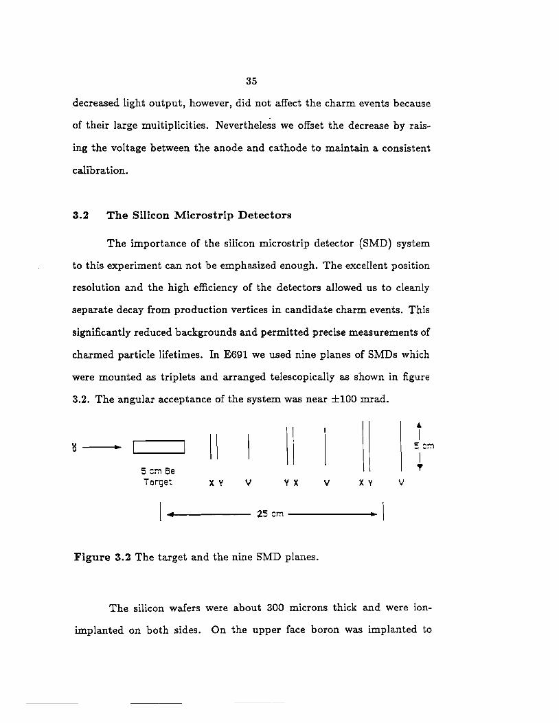
charmed particle lifetimes. In E691 we used nine planes of SMDs which
were mounted as triplets and arranged telescopically as shown in figure
3.2. The angular acceptance of the system was near ±100 mrad.
5 cm Be Terget
11
xv v v x
Figure 3.2 The target and the nine SMD planes.
v x y
' I 5cm
I T
v
The silicon wafers were about 300 microns thick and were ion-
implanted on both sides. On the upper face boron was implanted to
36
form p-type strips with a spacing of 50 microns above which a layer of
aluminum served as an ohmic contact. The bottom part of the silicon was
doped with a continuous n-type layer of arsenic over which aluminum was
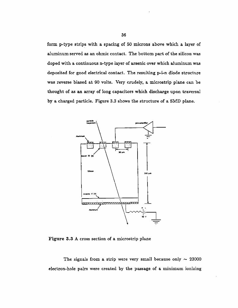
deposited for good electrical contact. The resulting p-i-n diode structure
was reverse biased at 90 volts. Very crudely, a microstrip plane can be
thought of as an array of long capacitors which discharge upon traversal
by a charged particle. Figure 3.3 shows the structure of a SMD plane.
trajKIOf'f partlele \
300µm
Figure 3.3 A cross section of a microstrip plane
The signals from a strip were very small because only ,_ 23000
electron-hole pairs were created by the passage of a minimum ionizing
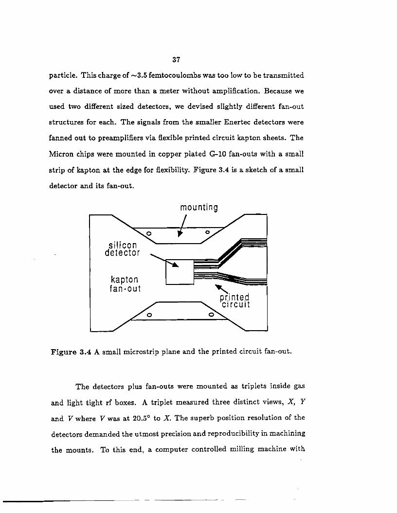
37
particle. This charge of ,_3.5 femtocoulombs was too low to be transmitted
over a distance of more than a meter without amplification. Because we
used two different sized detectors, we devised slightly different fan-out
structures for each. The signals from the smaller Enertec detectors were
fanned out to preamplifiers via flexible printed circuit kapton sheets. The
Micron chips were mounted in copper plated G-10 fan-outs with a small
strip of kapton at the edge for flexibility. Figure 3.4 is a sketch of a small
detector and its fan-out.
silicon detector
kapton fan-out
mounting
'· d pr.1 nte. c1rcu1t
Figure 3.4 A small microstrip plane and the printed circuit fan-out.
The detectors plus fan-outs were mounted as triplets inside gas
and light tight rf boxes. A triplet measured three distinct views, X, Y
and V where V was at 20.5° to X. The superb position resolution of the
detectors demanded the utmost precision and reproducibility in machining
the mounts. To this end, a computer controlled milling machine with
38
twelve micron precision was used to fabricate the mounts from Stesalit.
A special alignment jig was constructed with which the detectors were
properly aligned and then glued onto steel rings, or, in the case of the
Micron detectors, screwed onto internal Stesalit mounts. Between the
planes we maintained a relative rotati~nal offset about the beam axis of
less than 0.8 millirads. The construction arrangement was such that the
internal mounts fit perfectly into the external aluminum or copper plated
Stesalit rf boxes. The whole detector assembly was bolted to two optically
flat granite bars.
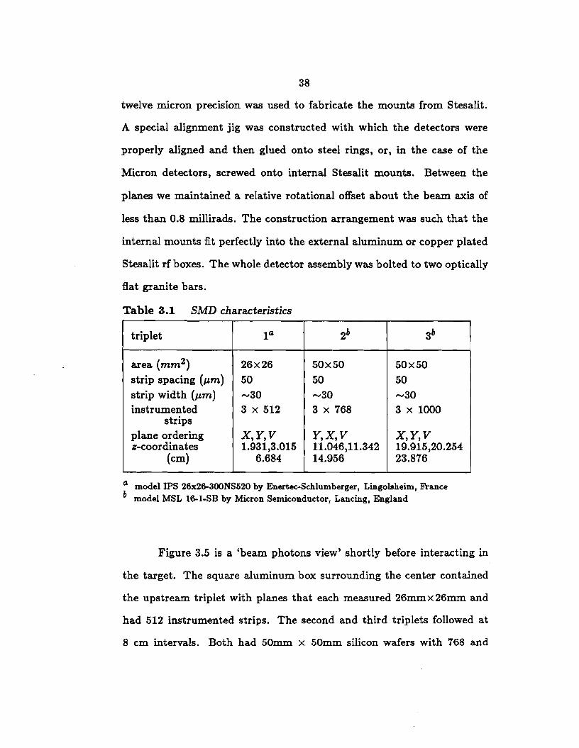
Table 3.1 SMD characteristics
triplet 1a 2b 3b
area (mm2) 26x26 50x50 50x50 strip spacing (µm) 50 50 50 strip width (µm) -30 -30 -30 instrumented 3 x 512 3 x 768 3 x 1000
strips plane ordering X,Y,V Y,X,V X,Y,V z-coordinates 1.931,3.015 11.046,11.342 19.915,20.254
(cm) 6.684 14.956 23.876
a model IPS 26x26-300NS520 by Enertec-Schlumberger, Lingolsheim, France b model MSL 16-1-SB by Micron Semiconductor, Lancing, England
Figure 3.5 is a 'beam photons view' shortly before interacting in
the target. The square aluminum box surrounding the center contained
the upstream triplet with planes that each measured 26mmx26mm and
had 512 instrumented strips. The second and third triplets followed at
8 cm intervals. Both had 50mm. x 50mm. silicon wafers with 768 and
39
1000 instrumented strips per wafer, respectively. Table 3.1 combines a
few characteristics of the SMDs. Figure 3.5 also shows the preamplifier
cages attached to the side of the rf shields. Each cage contained 32 four
channel preamp hybrids* which had a current gain of~ 200 and a risetime
~ 3 nanosecond. The cages were 9.5cm long, 3.0cm wide, 3.5cm deep and
were made from silver plated aluminum for good rf shielding.
The preamp signals were transmitted to the readout system in
4m long fiat shielded nine-channel cables, four and five for signal and
ground respectively. Channels carrying signals were sandwiched between
grounded strips to reduce crosstalk. The cables were shielded with alu-
minum foil which shared a common ground with the non-signal strips.
A good electrical contact was established by copper plating the ends of
the shield and by soldering the connection to ground. The readout sys
tem consisted of eight-channel MWPC discriminator cards, S710/810t,
stacked inside shielded cages. The cards were modified by the addition
of a transistor to invert the preamp output, and a potentiometer for ad-
justing the discriminator thresholds. For a minimum ionizing particle a
typical preamp signal was lm V. The discriminator levels were adjusted by
hand to about 0.5m V to cleanly separate the signals from the background.
The MWPC cards contained shift registers which were read out serially
with Camac scanners t.
The SMD detectors performed very well during the E691 data run.
* model MSD2 by Laben,Milan,Italy
t by Nanosystems Inc.,Oak Park,lliinois,USA
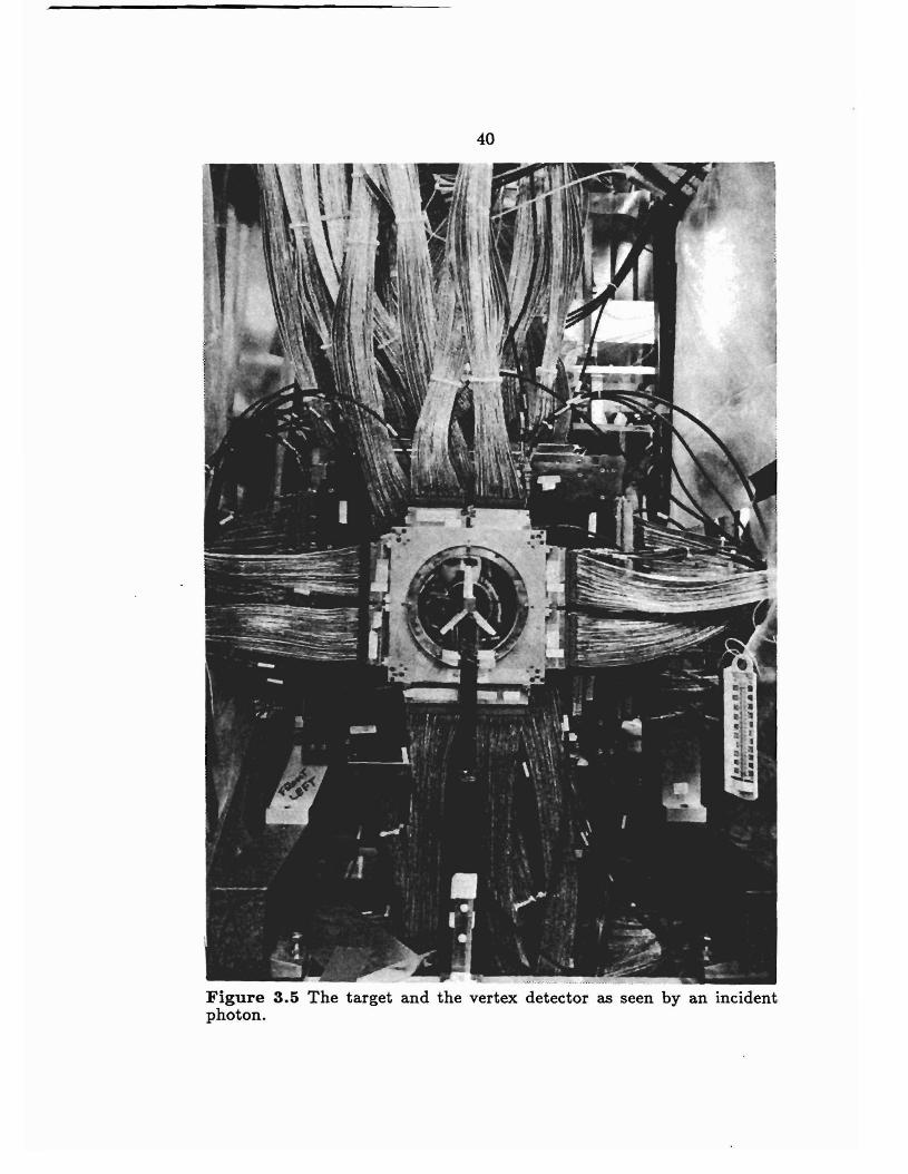
40
Figure 3.5 The target and the vertex detector as seen by an incident photon.
41
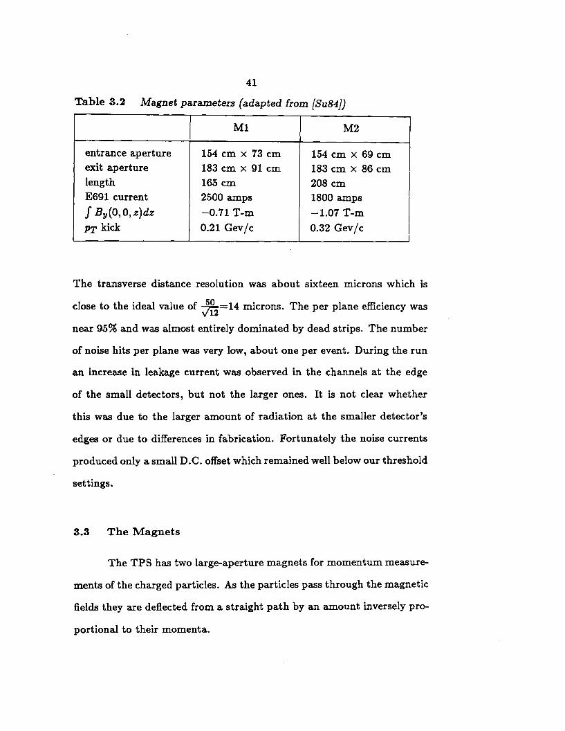
Table 3.2 Magnet parameters (adapted from {Su84})
Ml M2
entrance aperture 154 cm x 73 cm 154 cm x 69 cm exit aperture 183 cm x 91 cm 183 cm x 86 cm length 165 cm 208 cm E691 current 2500 amps 1800 amps
J By(O, 0, z)dz -0.71 T-m -1.07 T-m
PT kick 0.21 Gev/c 0.32 Gev/c
The transverse distance resolution was about sixteen microns which is
close to the ideal value of Jfu=14 microns. The per plane efficiency was
near 95% and was almost entirely dominated by dead strips. The number
of noise hits per plane was very low, about one per event. During the run
an increase in leakage current was observed in the channels at the edge
of the small detectors, but not the larger ones. It is not clear whether
this was due to the larger amount of radiation at the smaller detector's
edges or due to differences in fabrication. Fortunately the noise currents
produced only a small D.C. offset which remained well below our threshold
settings.
3.3 The Magnets
The TPS has two large-aperture magnets for momentum measure-
ments of the charged particles. As the particles pass through the magnetic
fields they are deflected from a straight path by an amount inversely pro-
portional to their momenta.
42
At TPL positive (negative) charged particles are bent to the east
(west). The total deflection angle is approximately given by
s~fB·dl 3.33p
with B in Tesla, p in Ge V / c and l in meters. Table 3.2 contains a few
general magnet parameters. The momentum resolution is proportional to
the position resolution Uz and v:aries with the field strength according to
[Fe86,Kl84]
lap I UzP p ~ .03B12·
To improve the momentum resolution we had to increase the magnetic
field because the Uz was already fixed by the position resolution of the
drift chambers and the l by the magnet drift chamber separation. The
magnet currents were increased from 1800 to 2500 amperes in the up-
stream magnet Ml and from 900 to 1800 amperes in the downstream
magnet M2. We used these currents since corresponding field maps from
E516 were available. The final horizontal PT kicks were 0.21 and 0.32
Ge V / c respectively.
Using the old maps from E516 along with a multiplicative scale
factor of 1.018, the Ks mass reconstructed from the decay Ks -+ 11"+11"-
was 498 MeV with a full width at half maximum (FWHM) of 7 MeV. We
also checked that the </> and A masses from the decays </> -+ K+ K- and
A -+ p11"- peaked in the proper places. Finally, we compared the mass
resolution in the data with that obtained in our Monte Carlo simulation.
For two track mass combinations the Monte Carlo consistently gave 10%
43
better resolution, but for three and four track combinations the differences
between the simulations and the data were negligible.
3.4 The Drift Chambers
For E691 we produced a very powerful charged particle detector. In
addition to the superb vertexing and tracking capabilities of the SMD's we
had four drift chamber stations with a total of 35 planes in front, between
and behind the magnets. In this way we followed the particles through
the spectrometer, measured their deflections by the magnetic fields and
thus their momenta, and projected them into the calorimeters to aid the
reconstruction there.
Drift chambers are position measuring devices, similar in readout
structure as the microstrip detectors-either a wire is hit or it isnt't. Here
electrons are liberated from a gas rather than a solid by the passage of a
charged particle. The electrons are forced to drift towards a sense wire
where they produce an avalanche which is collected. Appropriate voltages
on strategically located field-shaping wires guarantee that the electrons
drift towards the signal wires with almost constant velocity vd. From the
drift time, the time which passed between the passage of the particle and
the signal detection, one can extract the distance d of the particle from
the wire since d = vd~t. But note that a hit on a single wire gives no
information on which side of the wire the particle had passed.
The drift velocity can be selected through the drift gas and the
applied voltage. Independent of the chosen gas, it is essential that the
44
chamber be operated in the 'plateau region' where slight changes in field
strength do not produce significant changes in the drift velocity.
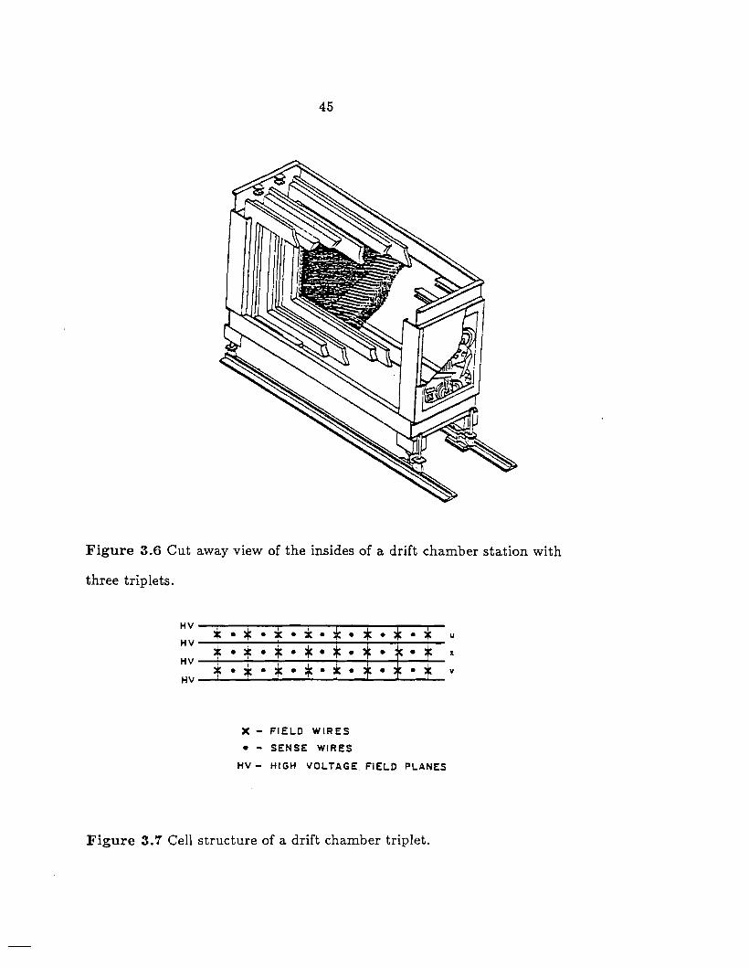
A typical drift chamber assembly is shown in figure 3.6. Up to
19 wire planes were stacked inside a large gas tight aluminum box with
mylar beam entrance and exit windows to minimize multiple scattering.
The planes alternated in their function, first a high voltage plane, then
a sense plane followed by another high voltage plane and so on. The
sense planes had wires strung vertically, and at ±20.5° to the vertical
for X, U and V position measurements. Every other wire was held at
a large negative potential to force electrons which had been liberated
to drift towards a grounded neighbouring sense wire. Figure 3. 7 shows
the arrangement of the planes. Typical operating voltages for our drift
chambers were between -2.1 and -2.6kV for the high voltage planes and
0.4-0.6kV higher for the field shaping wires.
We used equal parts of argon and ethane with a 1.5% admixture
of alcohol. The alcohol quenches the discharge, i.e., prevents sparks, and
thus reduces damage to the wires [Es86]. Our drift velocity was about
50µm/ns.
For the readout system we used LRS DC201 and N anomaker N-277C
discriminator-amplifier cards which were mounted on top of the chambers.
Twisted pair cables carried the output signals to LRS 4298 TDC's for dig
itization. The TDC gains were set to 1 count/nanosecond.
Upstream of the magnet Ml the SMD's and two chambers, DIA
45
Figure 3.6 Cut away view of the insides of a drift chamber station with
three triplets.
HV ~
HV
t HV
HV
I * . * . * . * • x . * . • . * . * . * t • •
I
* . * . . ~ . •
X - FIS:L.O WIRES
• - SENSE WIRES
t t: • •
* * *
HV - HIGH VOLTAGE FIEL.O PLANES
Figure 3. 7 Cell structure of a drift chamber triplet.
u
l
v
46
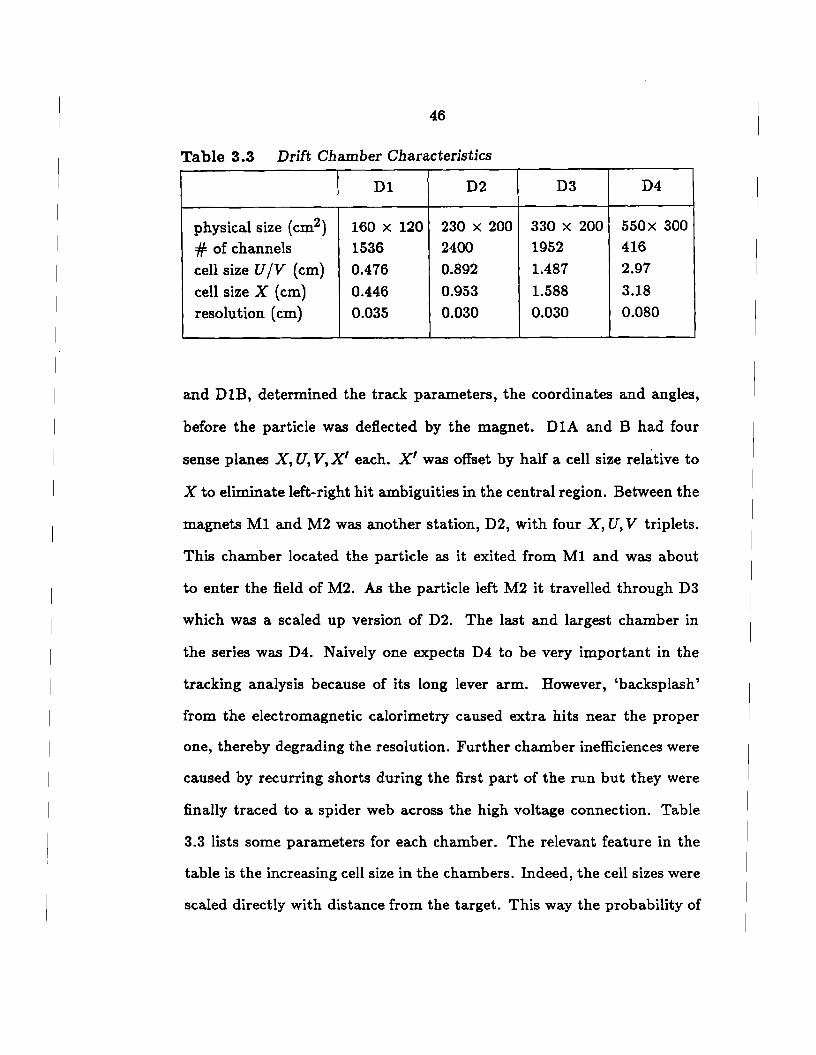
Table 3.3 Drift Chamber Characteristics
Dl D2 D3 D4
physical size (cm2) 160 x 120 230 x 200 330 x 200 550x 300
# of channels 1536 2400 1952 416
cell size U /V (cm) 0.476 0.892 1.487 2.97
cell size X (cm) 0.446 0.953 1.588 3.18
resolution (cm) 0.035 0.030 0.030 0.080
and DlB, determined the track parameters, the coordinates and angles,
before the particle was deflected by the magnet. DlA and B had four
sense planes X, U, V, X' each. X' was offset by half a cell size relative to
X to eliminate left-right hit ambiguities in the central region. Between the
magnets Ml and M2 was another station, D2, with four X, U, V triplets.
This chamber located the particle as it exited from Ml and was about
to enter the field of M2. As the particle left M2 it travelled through D3
which was a scaled up version of D2. The last and largest chamber in
the series was D4. Naively one expects D4 to be very important in the
tracking analysis because of its long lever arm. However, 'backsplash'
from the electromagnetic calorimetry caused extra hits near the proper
one, thereby degrading the resolution. Further chamber inefficiences were
caused by recurring shorts during the first part of the run but they were
finally traced to a spider web across the high voltage connection. Table
3.3 lists some parameters for each chamber. The relevant feature in the
table is the increasing cell size in the chambers. Indeed, the cell sizes were
scaled directly with distance from the target. This way the probability of
47
a hit in a particular cell was approximately constant.
The drift chamber calibration was done in two parts, on-line and
off-line. In the on-line calibration we subtracted constant time offsets, rel
ative t-zero's, while in the off-line calibration we oriented the drift chamber
planes with respect to each other and measured absolute t-zero's which
were plane to plane time offsets.
We split the raw TDC time count for each channel into three pieces,
where At was the drift time from the hit position to the signal wire. The
relative t-zero 's were measurements of the delay between the response to
a signal at the discriminator/ amplifier cards and a time displaced version
of the original pulser signal. The amount of retardation of the pulser
signal changed between plane assemblies. These time differences varied
from channel to channel due to differing cable lengths and slight variations
in electronic responses, but they were constant in time. The relative t
zero's were calculated at the beginning of every run, e.g., every 20-30
minutes. They were then written into the memory of the 4298 TDC crate
control unit for automatic internal subtraction. Thus, the subtraction of
the relative t-zero's produced a common reference time for the channels
within a single plane. The new TDC counts were
tT DO =traw - trel
=At+ tabs·
We obtained the absolute t-zero's and the chamber alignment con-
stants from a multi-parameter fit to clean muon tracks. The absolute
48
t-zeros were constant time offsets of the planes relative to the absolute
trigger signal. These offset are due to the different z positions of the
planes (e.g Dl TDC's counted time before 04 TDC's because the particle
got there earlier) and due to the fixed offsets in the relative t-zero calibra
tion. The alignment constants were simple spatial shifts from the internal
plane coordinate system to the overall drift chamber one. The fit to these
parameters, including the drift velocity vd, was identical in form to our
momentum fits. The data was obtained from special magnet-off muon
calibration runs that used a real beam trigger. For every muon track i
the fit minimized the following expression
where
QMDmi
was the mth plane's resolution
was the mth plane's offset
was the distance between the signaling sense wire and the center of the plane in the chamber coordinates
was the separation between the track and the sense wire in the plane's coordinates were the five track parameters: the x, y slopes, x, y intercepts and the track momentum were geometric factors needed to link the proper hits with these track parameters. Note: for magnet-off runs QMDms = 0
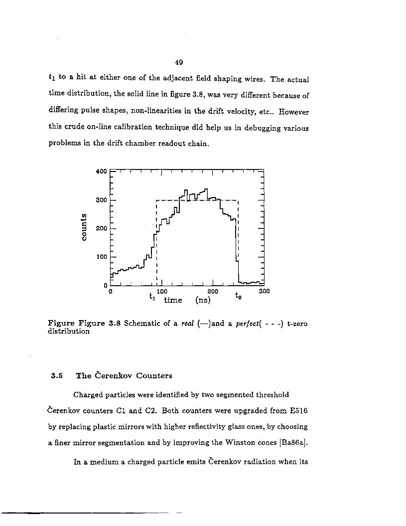
We also attempted to use an on-line procedure for determining
Toabs by looking at the raw time distributions of the muons. Under perfect
conditions these distributions would look as indicated by the dashed curve
in figure 3.8, where t2 corresponds to a direct hit on the sense wire and
49
t1 to a hit at either one of the adjacent field shaping wires. The actual
time distribution, the solid line in figure 3.8, was very different because of
differing pulse shapes, non-linearities in the drift velocity, etc .. However
this crude on-line calibration technique did help us in debugging various
problems in the drift chamber readout chain.
400
300
rn ~
§ 200 0 0
100
t 100 1 time
200 {ns)
300
Figure Figure 3-.8 Schematic of a real (-)and a per/ ect( - - -) t-zero distribution
3.5 The Cerenkov Counters
Charged particles were identified by two segmented threshold
Cerenkov counters Cl and C2. Both counters were upgraded from E516
by replacing plastic mirrors with higher reflectivity glass ones, by choosing
a finer mirror segmentation and by improving the Winston cones [Ba86aJ.
In a medium a charged particle emits Cerenkov radiation when its
50
speed exceeds that of the phase velocity of light. The number of photons
N emitted per unit wavelength A and unit length l is
(2)
where a ~ rl7 is the fine structure constant, p is the momentum of
the particle, Pth is the threshold momentum above which the particle can
radiate and 8 c is the Cerenkov angle, the angle between the direction of the
emitted radiation and the momentum vector. The threshold momentum
can be selected with the index of refraction n since
with E = n - 1.
c Vth = -
n
me Pth ~ y'2E'
Supposing that a momentum fit using the drift chamber informa
tion had found a particle of momentum p which did emit Cerenkov light,
the particle mass is then bounded above, m < J2E~. Similarly, the mass
would be bounded below if the particle had not radiated. Thus, from two
or more Cerenkov counters with distinct thresholds it is possible to set
bounds on particle masses and crudely distinguish between the particles
without detailed fits to the light cones.
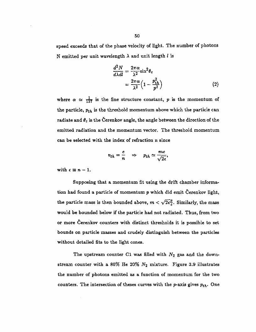
The upstream counter Cl was filled with N2 gas and the down
stream counter with a 80% He 20% N2 mixture. Figure 3.9 illustrates
the number of photons emitted as a function of momentum for the two
counters. The intersection of theses curves with the p-axis gives Pth· One
51
can deduce that with a 100% efficient light collection we should be able
to uniquely identify pions, kaons and protons in the 6-37, 20-37, 37-70
Ge V / c momentum regions, respectively.
40
_J
~ 30 z
20
10
125
100
_J 'l:l 75 ' z 'l:l
50
25
NUMBER OF PHOTONS PER METER VERSUS PARTICLE MOMENTA
C2
Cl
10 20 30 40 50 60 70 P(GeV/c)
Figure 3.9 Cerenkov light intensities versus momentum.
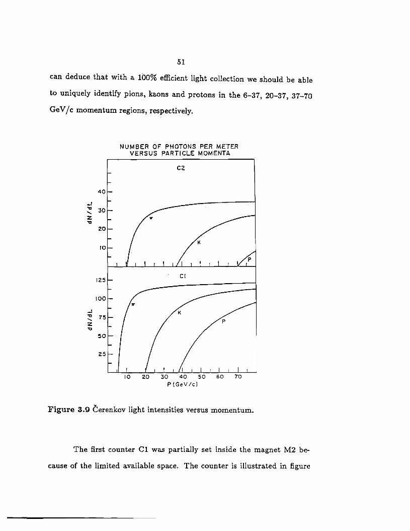
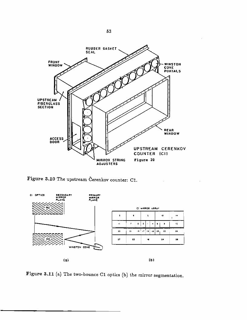
The first counter Cl was partially set inside the magnet M2 be-
cause of the limited available space. The counter is illustrated in figure
52
3.10. Twenty-eight mirrors focused Cerenkov light into their associated
Winston cones in the roundabout fashion depicted in figure 3.lla. This
'two-bounce' geometry was imposed by the space constraints of the spec
trometer. In Cl it was very important to have high reflectivity mirrors
because with 70% reflecting mirrors only 50% of the original light would
be left after the second reflection. In figure 3.llb we show the segmen
tation of the primary mirror plane. The finer segmentation in the center
minimized the probability of mirrors sharing light from two or more par
ticles.
A major draw back of the proximity of the magnet was the resid
ual magnetic field of up to two gauss at the photomultiplier tubes. Even
though the tubes were well shielded with cast iron piping, the field pen
etrated and deflected the electrons as they cascaded through the dyn
odes. This problem was partially rectified by winding current carrying
wire around the magnetic shields to cancel the fields.
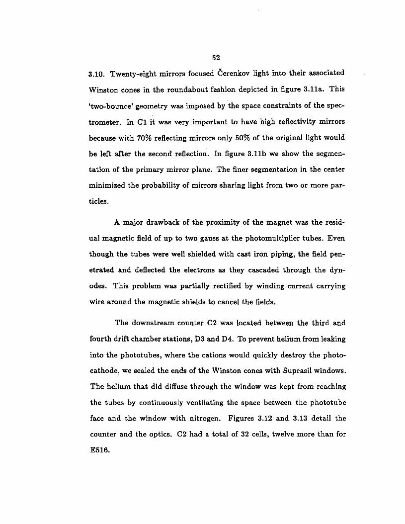
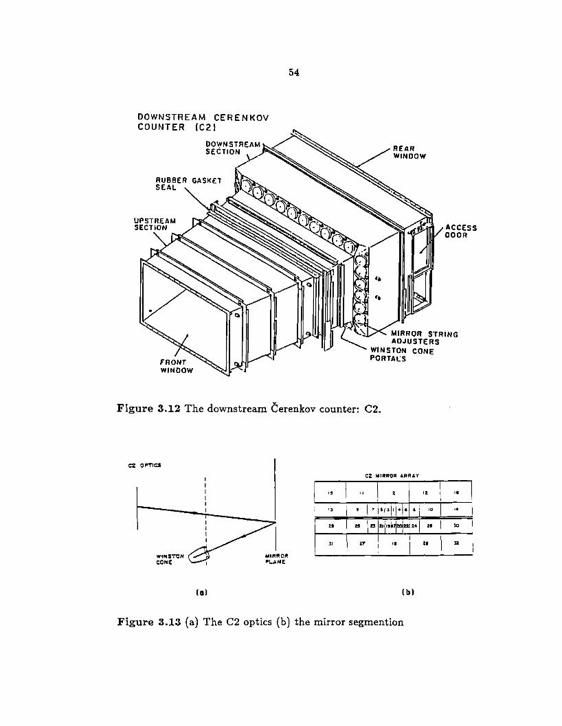
The downstream counter C2 was located between the third and
fourth drift chamber stations, D3 and D4. To prevent helium from leaking
into the phototubes, where the cations would quickly destroy the photo
cathode, we sealed the ends of the Winston cones with Suprasil windows.
The helium that did diffuse through the window was kept from reaching
the tubes by continuously ventilating the space between the phototube
face and the window with nitrogen. Figures 3.12 and 3.13 detail the
counter and the optics. C2 had a total of 32 cells, twelve more than for
E516.
FRONT WINDOW
RUBBER SEAL
53
MIRROR STRING ADJUSTERS
UPSTREAM CERENKOV COUNTER (Cl) Figure 20
Figure 3.10 The upstream Cerenkov counter: Cl.
C:I OPTICS S!CONOARY MIRROR Pl.AN£
~I
(a)
~"!MARY MIRROR Pl,.ANE
13 ' II 1
Z5 ZI
Z7 u
Cl MIRROR ARRAY
i 10
1. 14
I , 3 I ' ' a I IZ
' ,, i 11 15 18 zo zz 2.15
1• Z4 za
(b)
Figure 3.11 (a) The two-bounce Cl optics (b) the mirror segmentation.
I I
54
DOWNSTREAM CERENKOV COUNTER (C2)
ACCESS DOOR
MIRROR STRING ADJUSTERS
WINSTON CONE PORTAlS
Figure 3.12 The downstream Cerenkov counter: C2.
C2 OPTICS
WINSTON CONE
(a)
MIRROR Fl\.ANE
IS
13 I H
31
C2 MIRROR ARRAY
II z
' I , s l Ir 4 ' • I
u \ u ZI 1'r1 tzc zzj 24
ZT' ••
(b)
Figure 3.13 (a) The C2 optics (b) the mirror segmention
IZ II
10 14
21 30 I
ZI ll
55
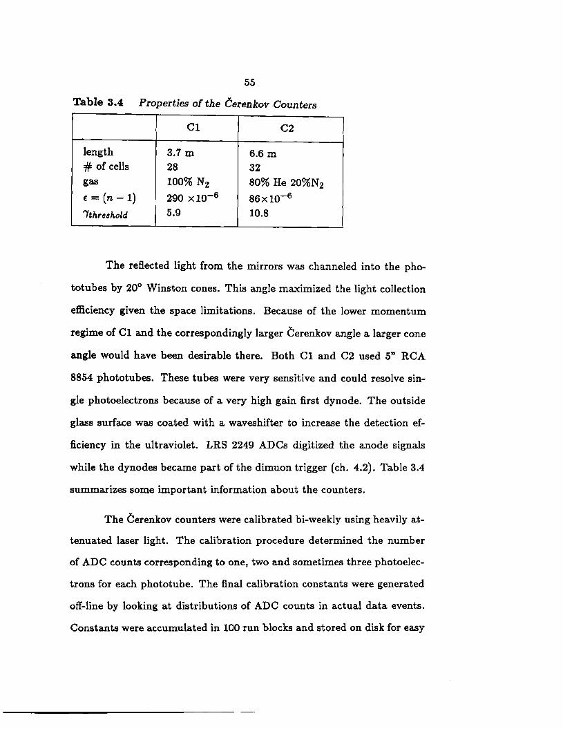
Table 3.4 Properties of the Cerenkov -Counters
Cl C2
length 3.7 m 6.6m #of cells 28 32 gas 100% N2 80% He 20%N2 E = (n -1) 290 x10-6 86x10-6
I threshold 5.9 10.8
The reflected light from the mirrors was channeled into the pho
totubes by 20° Winston cones. This angle maximized the light collection
efficiency given the space limitations. Because of the lower momentum
regime of Cl and the correspondingly larger Cerenkov angle a larger cone
angle would have been desirable there. Both Cl and C2 used 5" RCA
8854 phototubes. These tubes were very sensitive and could resolve sin-
gle photoelectrons because of a very high gain first dynode. The outside
glass surface was coated with a waveshifter to increase the detection ef-
ficiency in the ultraviolet. LRS 2249 ADCs digitized the anode signals
while the dynodes became part of the dimuon trigger (ch. 4.2). Table 3.4
summarizes some important information about the counters.
The Cerenkov counters were calibrated bi-weekly using heavily at
tenuated laser light. The calibration procedure determined the number
of ADC counts corresponding to one, two and sometimes three photoelec-
trons for each phototube. The final calibration constants were generated
off-line by looking at distributions of ADC counts in actual data events.
Constants were accumulated in 100 run blocks and stored on disk for easy
56
access by the reconstruction programs. We found that the number of
photoelectrons collected per track was ,....,11 in Cl and ,....,13 in C2.
3.6 The Calorimeters
The TPS has two large calorimeters, a segmented lead interleaved
calorimeter for electromagnetic shower detection and an iron scintillator
sandwich for hadronic energy measurements. For E691, the calorimeters
served not only as neutral particle detectors, but also as inputs to the
main trigger-a large transverse energy trigger.
3.6.l The Electromagnetic Shower Calorimeter
A large liquid scintillator calorimeter, the SLIC [Bh78,Bh85], was
used to detect electrons and photons. With the SLIC it was possible to
distinguish electrons from charged hadrons by their respectively narrow
and wide shower widths. We reconstructed 1r0 's and 71's from photons
which produced neutral and distinctively thin showers. The SLIC also
provided the electromagnetic component to the main trigger.
Bremsstrahlung together with pair production is used to observe
high energy photons and electrons. When electrons pass through a thick
material they radiate photons that convert to electron-positron pairs which
in turn radiate ... and so on. This showering process stops when the pho
ton energy falls below 1 MeV, the threshold for e+e- production. Never
theless, the photons and electrons continue to lose energy through various
interactions, i.e. ionization and Compton scattering. To detect the ra-
57
diation with ordinary photomultiplier tubes the radiator is followed by a
scintillator which absorbs energy over a wide band but emits only in a
narrow regime. The scintillation light is channeled to the phototubes via
totally internally reflecting light guides. The amount of light collected
is proportional to the energy of the incident electromagnetic particle, as
suming that little has leaked out of the detector. The collection efficiency
can be increased by adding a wave shifting material to the scintillator to
reduce self-absorption and to shift the light into the high efficiency domain
of the photomultiplier.
The SLIC was basically a large tank filled with liquid scintilla
tor. Sixty layers of 0.63cm thick flat lead and thin corrugated aluminum
sheets were stacked as shown in figure 3.14. Because of the high Z, lead
has large electromagnetic cross sections and is thus very suitable for ini
tiating and maintaining the s}_iowering process. From figure 3.16 one can
see how the corrugations formed the U, V and Y channels. The Y view
was split into east and west halves of 58 channels each. The 109 U and
109 V channels were read out at the top and bottom, respectively. The
aluminum corrugations were coated with a thin layer of teflon. Because
of the lower index of refraction of teflon relative to that of the scintillator,
light waves with angles of incidence less than about 20° were completely
reflected. The channels were 6.4cm wide except in the congested central
region where better position resolution was needed to resolve the individ
ual showers; there they were 3.2cm wide. The ultraviolet light emitted by
the liquid scintillator-waveshifter combination was collected at the edges
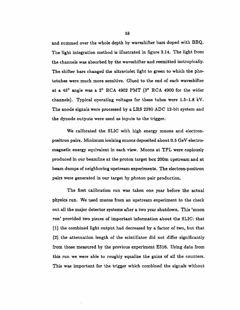
58
and summed over the whole depth by waveshifter bars doped with BBQ.
The light integration method is illustrated in figure 3.14. The light from
the channels was absorbed by the waveshifter and reemitted isotropically.
The shifter bars changed the ultraviolet light to green to which the pho
totubes were much more sensitive. Glued to the end of each waveshifter
at a 45° angle was a 2" RCA 4902 PMT {3" RCA 4900 for the wider
channels). Typical operating voltages for these tubes were 1.5-1.8 kV.
The anode signals were processed by a LRS 2280 ADC 12-bit system and
the dynode outputs were used as inputs to the trigger.
We calibrated the SLIC with high energy muons and electron
positron pairs. Minimum ionizing muons deposited about 0.5 Ge V electro
magnetic energy equivalent in each view. Muons at TPL were copiously
produced in our beamline at the proton target box 200m upstream and at
beam dumps of neighboring upstream experiments. The electron-positron
pairs were generated in our target by photon pair production.
The first calibration run was taken one year before the actual
physics run. We used muons from an upstream experiment to the check
out all the major detector systems after a two year shutdown. This 'muon
run' provided two pieces of important information about the SLIC: that
(1) the combined light output had decreased by a factor of two, but that
(2) the attenuation length of the scintillator did not differ significantly
from those measured by the previous experiment E516. Using data from
this run we were able to roughly equalize the gains of all the counters.
This was important for the trigger which combined the signals without
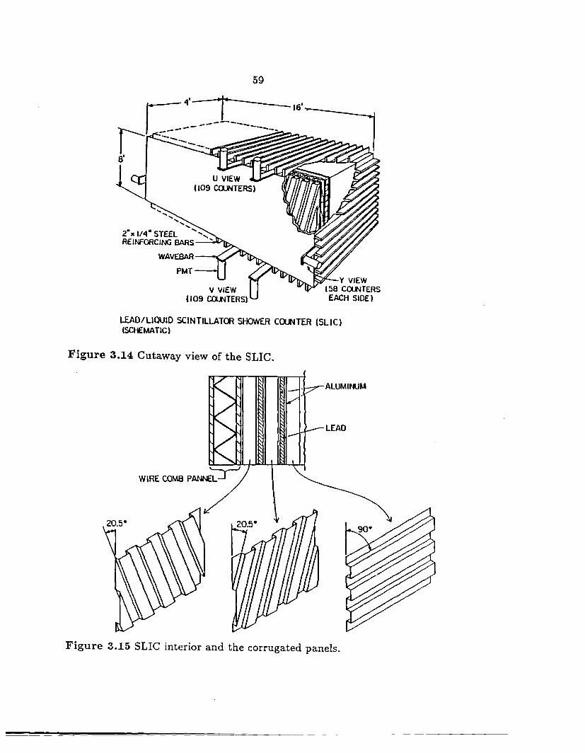
59
LEAD/LIOUIO SCJNTILLATOO SHOWER CCl.JNTER (SLJC) (SCHEMA TIC)
Figure 3.14 Cutaway view of the SLIC.
Figure 3.15 SLIC interior and the corrugated panels.
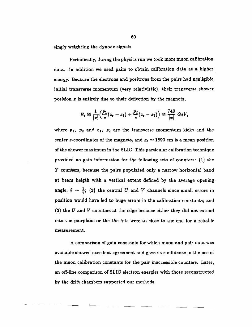
60
singly weighting the dynode signals.
Periodically, during the physics run we took more muon calibration
data. In addition we used pairs to obtain calibration data at a higher
energy. Because the electrons and positrons from the pairs had negligible
initial transverse momentum (very relativistic), their transverse shower
position :r; is entirely due to their deflection by the magnets,
,..., 1 (Pl P2 ) ,..., 7 40 Ee= j;"j ~(z., - z1) + ~(z., - z2) = j;I GeV,
where P1, P2 and zi, z2 are the transverse momentum kicks and the
center z-coordinates of the magnets, and z8 ~ 1890 cm is a mean position
of the shower maximum in the SLIC. This particular calibration technique
provided no gain information for the following sets of counters: (1) the
Y counters, because the pairs populated only a narrow horizontal band
at beam heigth with a vertical extent defined by the average opening·
angle, fJ ,..,, ~; (2) the central U and V channels since small errors in
position would have led to huge errors in the calibration constants; and
(3) the U and V counters at the edge because either they did not extend
into the pairplane or the the hits were to close to the end for a reliable
measurement.
A comparison of gain constants for which muon and pair data was
available showed excellent agreement and gave us confidence in the use of
the muon calibration constants for the pair inaccessible counters. Later,
an off-line comparison of SLIC electron energies with those reconstructed
by the drift chambers supported our methods.
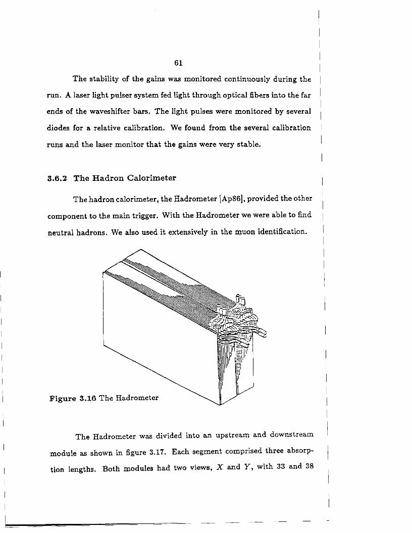
61
The stability of the gains was monitored continuously during the
run. A laser light pulser system fed light through optical fibers into the far
ends of the waveshifter bars. The light pulses were monitored by several
diodes for a relative calibration. We found from the several calibration
runs and the laser monitor that the gains were very stable.
3.6.2 The Hadron Calorimeter
The hadron calorimeter, the Hadrometer [ Ap86], provided the other
component to the main trigger. With the Hadrometer we were able to find
neutral hadrons. We also used it extensively in the muon identification.
Figure 3.16 The Hadrometer
The Hadrometer was divided into an upstream and downstream
module as shown in figure 3.17. Each segment comprised three absorp
tion lengths. Both modules had two views, X and Y, with 33 and 38
62
counters/module respectively. The Y views were, as in the SLIC, divided
into an east and west half. The scintillator light was shifted into the visi
ble and converted to an electronic signal by 5" EMI 9791KB phototubes.
The tubes were glued directly onto the lightguides. The anode signals
were digitized by a second LRS 2280 ADC system and the dynodes were
fanned together for the triggers. The ADC gains for the Hadrometer were
set to twice the SLIC ADC gains since the signals were weaker. A typical
ADC gain was about 20 counts/GeV.
The Hadrometer, like the SLIC, sampled and summed the energy
content of the showers at various depths of the material. The hadronic
shower characteristics differ from electromagnetic ones because the in
teractions tend to produce high energy secondaries with large transverse
momenta. Thus hadronic showers are wider and take longer to develop
longitudinally. Indeed, the majority of hadronic showers were born in the
SLIC but contained in the Hadrometer.
The Hadrometer and SLIC muon calibration data were recorded
simultaneously. Each muon left on the average 2.4 Ge V hadron equivalent
energy in the calorimeter (1.2 GeV /channel). This typical signal size and
the skinny 'shower' of the muon was later used in the reconstruction for
identification. To obtain the gains Ui for each channel i we fitted the signal
distributions Ii in each counter to
Ii ( x) = Ui ( 1 + ai e - :, ) ,
with x the distance from the muon hit to the photomultiplier tube. The
gain Ui and the attenuation length parameters, ai and .\i, were allowed
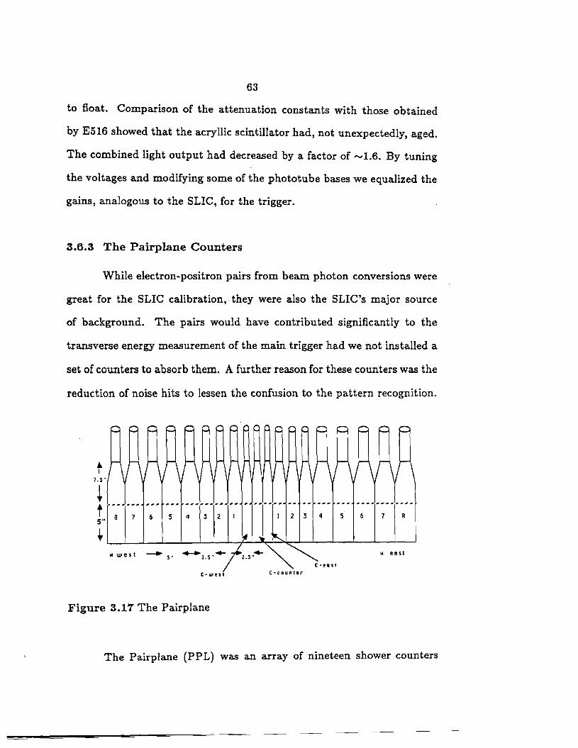
63
to float. Comparison of the attenuation constants with those obtained
by E516 showed that the acryllic scintillator had, not unexpectedly, aged.
The combined light output had decreased by a factor of -1.6. By tuning
the voltages and modifying some of the phototube bases we equalized the
gains, analogous to the SLIC, for the trigger.
3.6.3 The Pairplane Counters
While electron-positron pairs from beam photon conversions were
great for the SLIC calibration,· they were also the SLIC's major source
of background. The pairs would have contributed significantly to the
transverse energy measurement of the main trigger had we not installed a
set of counters to absorb them. A further reason for these counters was the
reduction of noise hits to lessen the confusion to the pattern recognition.
t 7. s.
i t S" B 6 s 4 3 2 I 23 4 S 6 7 8
·L--~J.--~_._~~---1-.-..-~~__._-----~-------~ H west __.
5• M eest
c-west
Figure 3.17 The Pairplane
The Pairplane (PPL) was an array of nineteen shower counters
64
as illustrated in figure 3.17. The detectors were supported by a shelf at
beam height directly in front of the SLIC. The shelf could be raised for
SLIC calibration runs. The central three counters Cea8t, Ccenter and Cwest
were supposed to measure the energy of other photons that were created
during the bremsstrahlung of the electron in the tungsten r~diatior. The
C-counters, XEl-3 and XWl-3 were tungsten-lucite sandwiches while the
other ten counters were made from lead and lucite layers. To insure almost
complete absorption of the beam pairs and the beam photons the total
thickness of the pairplane was fixed at -20 radiation lengths followed
by an additional IO radiation lengths of lead brick. The readout system
consisted of RCA 6342 photomultipliers which were chosen for their ability
to perform well in high rate environments, and LRS 2249 ADCs to digitize
the anode signals. The dynodes were used as inputs to the calibration
trigger.
The C-counters were calibrated twice at the beginning of the data
run with 50 and 200 GeV /c electrons obtained by removing the tungsten
radiator and the beryllium target. The 50 GeV /c beam was then steered
into the counters with the tagging magnets. The other counters were
calibrated on-line and off-line with e+e- pairs. The method was identical
to that used for the SLIC calibration, except for the constant relating the
energy and position,
680 Ee~ j;f GeV
Off-line, the energy deposits in the PPL were also compared to drift cham-
her energies. For unknown reasons the PPL proved very inefficient in de-
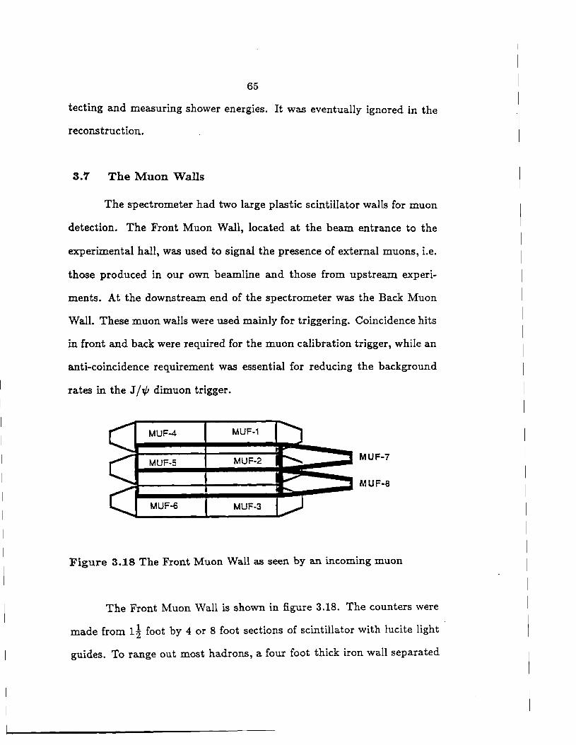
65
tecting and measuring shower energies. It was eventually ignored in the
reconstruction.
3.T The Muon Walls
The spectrometer had two large plastic scintillator walls for muon
detection. The Front Muon Wall, located at the beam entrance to the
experimental hall, was used to signal the presence of external muons, i.e.
those produced in our own beamline and those from upstream experi
ments. At the downstream end of the spectrometer was the Back Muon
Wall. These muon walls were used mainly for triggering. Coincidence hits
in front and back were required for the muon calibration trigger, while an
anti-coincidence requirement was essential for reducing the background
rates in the J / tf; dimuon trigger.
MUF-4 MUF-1
MUF-5 MUF-2 MUF-7
MUF-8
MUF-6 MUF-3
Figure 3.18 The Front Muon Wall as seen by an incoming muon
The Front Muon Wall is shown in figure 3.18. The counters were
made from 1 ~ foot by 4 or 8 foot sections of scintillator with lucite light
guides. To range out most hadrons, a four foot thick iron wall separated
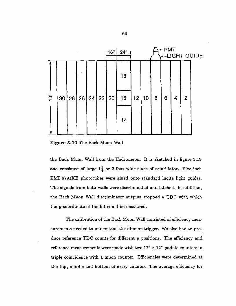
66
UIDE l)s·:j 24" ·I -PMT -LIGHT G
18
30 28 26 24 22 20 16 12 10 8 6 4 2 0 T"'""
14
Figure 3.19 The Back Muon Wall
the Back Muon Wall from the Hadrometer. It is sketched in figure 3.19
and consisted of large 1 i or 2 foot wide slabs of scintillator. Five inch
EMI 9791KB phototubes were glued onto standard lucite light guides.
The signals from both walls were discriminated and latched. In addition,
the Back Muon Wall discriminator outputs stopped a TDC with which
they-coordinate of the hit could be measured.
The calibration of the Back Muon Wall consisted of efficiency mea-
surements needed to understand the dimuon trigger. We also had to pro-
duce reference TDC counts for different y positions. The efficiency and
reference measurements were made with two 12" x 12" paddle counters in
triple coincidence with a muon counter. Efficiencies were determined at
the top, middle and bottom of every counter. The average efficiency for
67
the back counters was ....... 94 % with typical counter noise rates in the MHz
range.
Not shown in figure 3.19 are the two Caboose counters which were
mounted on the back of a three foot thick concrete block behind the
center of the back wall. Logical ANDs made with the center counter
and the Caboose reduced false dimuon triggers from outside muons. A
large number of these false triggers was caused by the overlap of the light
guide of the lower center counter with the middle one. We placed another
counter, MU141, over the lower one to eliminate this problem.
In summary of this long chapter, all the major components of the
spectrometer are listed in table 3.5.
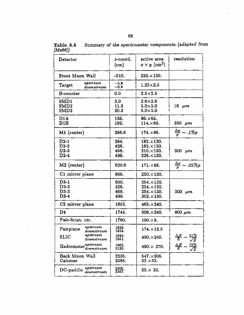
68
Table 3.5 {Me86})
Summary of the spectrometer components (adapted from
Detector z-coord. active area resolution (cm) xx y (cm2)
Front Muon Wall -510. 250.x150.
Target upstream -5.8 1.25x2.5 downstream -0.8
B-counter 0.0 2.5x2.5
SMDl 3.0 2.6x2.6 SMD2 11.3 5.0x5.0 16 µm SMD3 20.3 5.0x5.0
DIA 156. 86.x65. DlB 192. 114.x65. 350 µ,m
Ml (center) 286.6 174.x86. ~ ,_ .1%p
D2-1 384. 182.x130. D2-2 426. 182.x130. D2-3 468. 210.x130. 300 µm D2-4 499. 228.x130.
M2 (center) 620.6 171. x88. ~ ,_ .05%p
Cl mirror plane 866. 250.x130.
D3-1 930. 254.x130. D3-2 426. 254.x130. D3-3 468. 254.x130. 300 µm D3-4 499. 302.x130.
C2 mirror plane 1653. 465.x240.
D4 1744. 508.x240. 800 µ,m
Pair-Scint. ctr. 1760. 100.xS.
Pairplane upstream 1829. 174.x 12.5 downstream 1839.
SLIC upstream 1849. 490.x240. l::.E 21% downstream 1951. T,_ VE
H d upstream 1962. 490.x 270. t:.E 12% a rometer downstream 2120. T,_ VE
Back Muon Wall 2235. 547.x305. Caboose 2385. 33.x33.
DC ddl upstream 2300. 33.x 33. -pa e downstream 2367.
69
4 The Data Collection
The data collection system had three components: the triggers,
the data acquisition, and the data monitor. Because typical interaction
rates in the experiment were on the order of 10000 /second and char~
rates 1/second, we needed a fast, selective, and charm efficient trigger.
From a sum of the calorimeter signals we estimated the hadronic energy
and transverse energy of the event. On the basis of these two pieces of
information we rejected about 99% of the events while retaining 80% of
the charm. Upon receipt of a trigger, a PDP-11 initiated a digitization
sequence in the TDC's and ADC's. The events were then read out by the
PDP-11 via CAMAC and recorded on magnetic tape. We matched the
trigger rates to the data handling capabilities of the the PDP. A small
fraction of the events were passed to a VAX 11/780 for monitoring the
experiment as a whole and for performing detailed checks on the detectors.
4.1 The Triggers
In E691 we had three distinct trigger types: physics, calibration
and monitoring triggers; The physics and calibration triggers used real
beam and therefore were active only for the 22 second spill in the 60
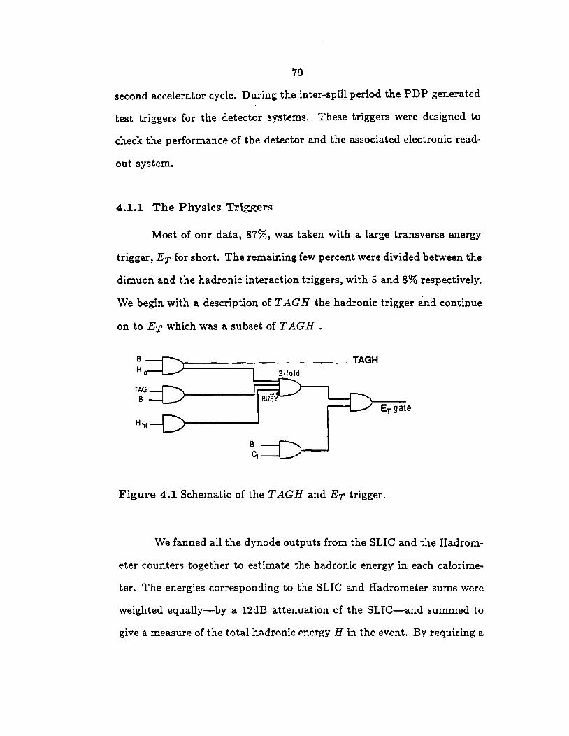
70
second accelerator cycle. During the inter-spill period the PDP generated
test triggers for the detector systems. These triggers were designed to
check the performance of the detector and the associated electronic read-
out system.
4.1.1 The Physics Triggers
Most of our data, 87%, was taken with a large transverse energy
trigger, Ex for short. The remaining few percent were divided between the
dimuon and the hadronic interaction triggers, with 5 and 8% respectively.
We begin with a description of TAG H the hadronic trigger and continue
on to ET which was a subset of TAGH.
TAG B
Figure 4.1 Schematic of the T AGH and ET trigger.
We fanned all the dynode outputs from the SLIC and the Hadrom-
eter counters together to estimate the hadronic energy in each calorime-
ter. The energies corresponding to the SLIC and Hadrometer sums were
weighted equally-by a 12dB attenuation of the SLIC-and summed to
give a measure of the total hadronic energy H in the event. By requiring a
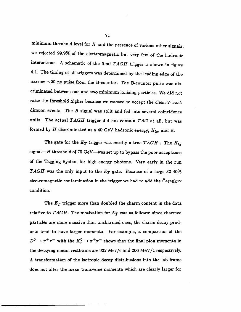
71
minimum threshold level for Hand the presence of various other signals,
we rejected 99.9% of the electromagnetic but very few of the hadronic
interactions. A schematic of the final T AGH trigger is shown in figure
4.1. The timing of all triggers was determined by 'the leading edge of the
narrow -20 ns pulse from the B-counter. The B-counter pulse was dis
criminated between one and two minimum ionizing particles. We did not
raise the threshold higher because we wanted to accept the clean 2-track
dimuon events. The B signal was split and fed into several coincidence
units. The actual TAG H trigger did not contain TAG at all, but was
formed by H discriminated at a 40 GeV hadronic energy, Hlo, and B.
The gate for the ET trigger was mostly a true TAG H . The H hi
signal-H threshold of 70 Ge V-was set up to bypass the poor acceptance
of the Tagging System for high energy photons. Very early in the run
TAG H was the only input to the ET gate. Because of a large 30-40%
electromagnetic contamination in the trigger we had to add the Cerenkov
condition.
The ET trigger more than doubled the charm content in the data
relative to TAGH. The motivation for ET was as follows: since charmed
particles are more massive than uncharmed ones, the charm decay prod
ucts tend to have larger momenta. For example, a comparison of the
Do~ 11"+11"- with the K~ ~ 11"+11"- shows that the final pion momenta in
the decaying meson restframe are 922 Mev / c and 206 Me V / c respectively.
A transformation of the isotropic decay distributions into the lab frame
does not alter the mean transverse momenta which are clearly larger for
72
charm. We studied this effect as applied to the Tagged Photon Spectrom
eter with Monte Carlo simulations and data from the preceeding exper
iment, and found that a significant charm enrichment could be obtained
by triggering on high PT particles. We illustrate the difference in PT or
equivalently ET between all hadrons and charm in figures 4.2 and 4.3.
250
200
~'''~~~ tn 150 ., c:
11 ~~ I ~ rz1 100
I \111~ I 60 ~ ' , ,
f t ~,,~
•' f ••••• 0 0 2 4
ET (GeV)
Figure 4.2 ET distribution in hadronic events for TAGH data.
20
10
0 .......... _._..._.1-.1-.i......i;.""""-...__ ........ __,.. ....
0 2 4 e E,. (GeV)
Figure 4.3 ET distribution for charm events in TAGH data.
Considering that there were 104 interactions/ second, the decision
to record an event had to be made within tens of microseconds. Since
CAMAC readout times were on the order of milliseconds a partial on-line
reconstruction was out of the question. For us, the simplest trigger to im-
plement was one based on a calorimetric transverse energy measurement.
Large PT particles have, on the average, large angles relative to the beam
axis so that they interact in the calorimeters far from the beam center.
Thus, the trigger had to weight the energy deposits in proportion to their
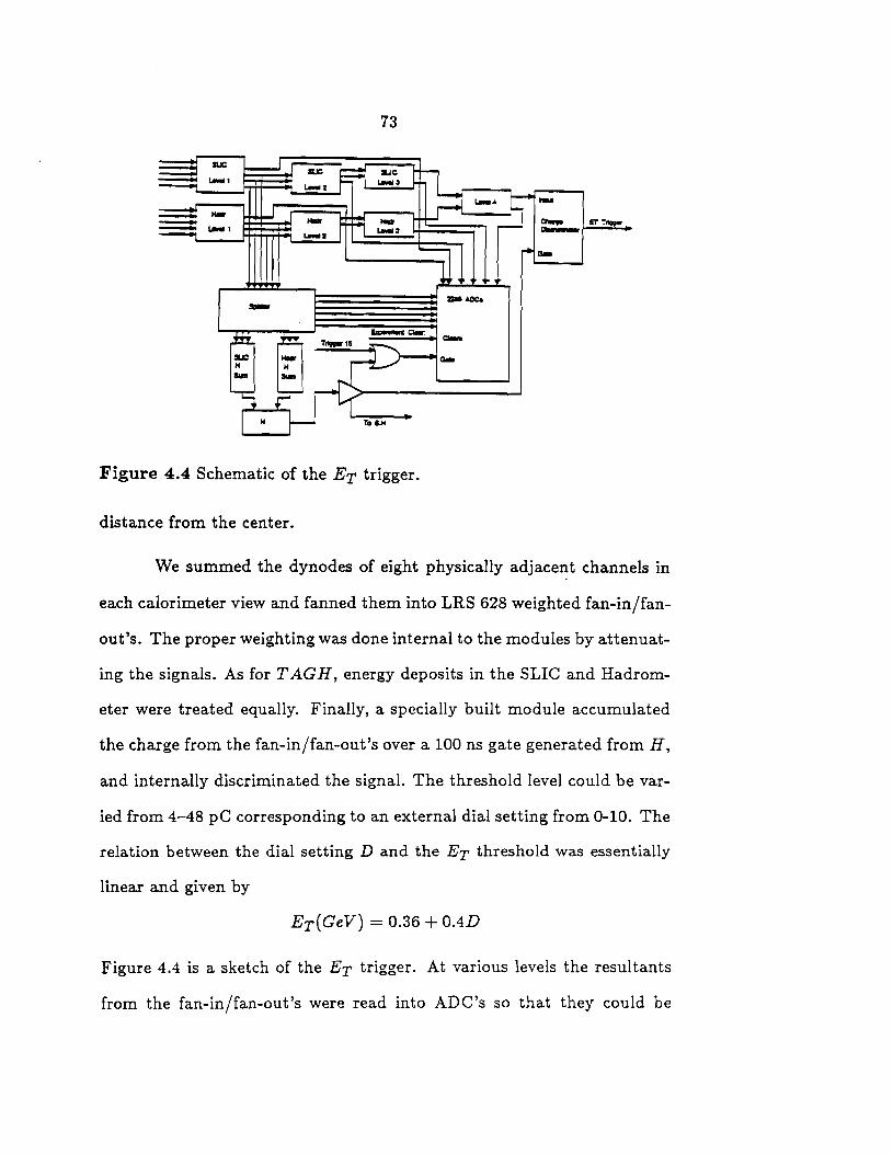
73
=== sue sue i...1
u-12
.... -.... - Mlllr - lalMI 1 La92
Figure 4.4 Schematic of the ET trigger.
distance from the center.
We summed the dynodes of eight physically adjacent channels in
each calorimeter view and fanned them into LRS 628 weighted fan-in/fan
out's. The proper weighting was done internal to the modules by attenuat-
ing the signals. As for T AGH, energy deposits in the SLIC and Hadrom~
eter were treated equally. Finally, a specially built module accumulated
the charge from the fan-in/fan-out's over a 100 ns gate generated from H,
and internally discriminated the signal. The threshold level could be var-
ied from 4-48 pC corresponding to an external dial setting from 0-10. The
relation between the dial setting D and the ET threshold was essentially
linear and given by
ET(GeV) = 0.36 + 0.4D
Figure 4.4 is a sketch of the ET trigger. At various levels the resultants
from the fan-in/fan-out's were read into ADC's so that they could be
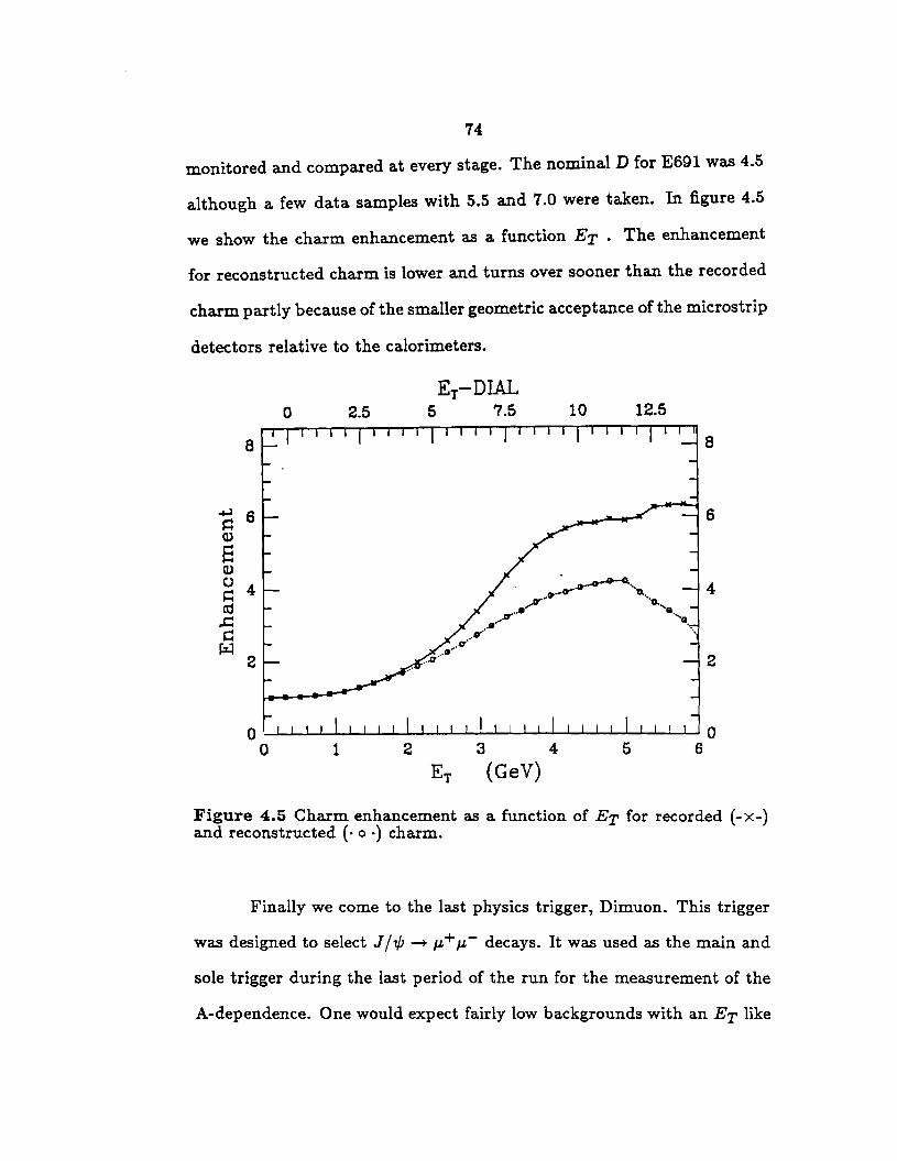
74
monitored and compared at every stage. The nominal D for E691was4.5
although a few data samples with 5.5 and 7.0 were taken. In figure 4.5
we show the charm enhancement as a function ET • The enhancement
for reconstructed charm is lower and turns over sooner than the recorded
charm partly because of the smaller geometric acceptance of the microstrip
detectors relative to the calorimeters.
Er-DIAL 0 2.5 5 7.5 10 12.5
a a
6
4
2 2
0 ._._ ___ ....._.. ___ ..-..._._ ................. _._. ............ _..._..,,__._._-'"-~-'-.._.,--'-..l..-L-l...-L.....J 0 0 1 2 3 4 5 6
Er (GeV)
Figure 4.5 Charm enhancement as a function of ET for recorded (-x-) and reconstructed ( · o ·) charm.
Finally we come to the last physics trigger, Dimuon. This trigger
was designed to select Jft/J--.. µ+µ-decays. It was used as the main and
sole trigger during the last period of the run for the measurement of the
A-dependence. One would expect fairly low backgrounds with an ET like
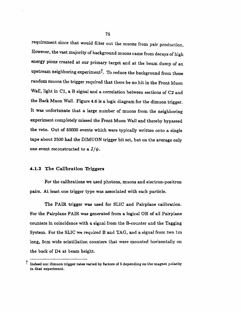
75
requirement since that would filter out the muons from pair production.
However, the vast majority of background muons came from decays of high
energy pions created at our primary target and at the beam dump of an
upstream neighboring experiment t. To reduce the background from these
random muons the trigger required that there be no hit in the Front Muon
Wall, light in Cl, a B signal and a correlation between sections of C2 and
the Back Muon Wall. Figure 4.6 is a logic diagram for the dimuon trigger.
It was unfortunate that a large number of muons from the neighboring
experiment completely missed the Front Muon Wall and thereby bypassed
the veto. Out of 50000 events which were typically written onto a single
tape about 2500 had the DIMUON trigger bit set, but on the average only
one event reconstructed to a J / ,,P.
4.1.2 The Calibration Triggers
For the calibrations we used photons, muons and electron-positron
pairs. At least one trigger type was associated with each particle.
The PAIR trigger was used for SLIC and Pairplane calibration.
For the Pairplane PAIR was generated from a logical OR of all Pairplane
counters in coincidence with a signal from the B-counter and the Tagging
System. For the SLIC we required Band TAG, and a signal from two Im
long, 5cm wide scintillation counters that were mounted horizontally on
the back of D4 at beam height.
t Indeed our dimuon trigger rates varied by factors of 5 depending on the magnet polarity in that experiment.
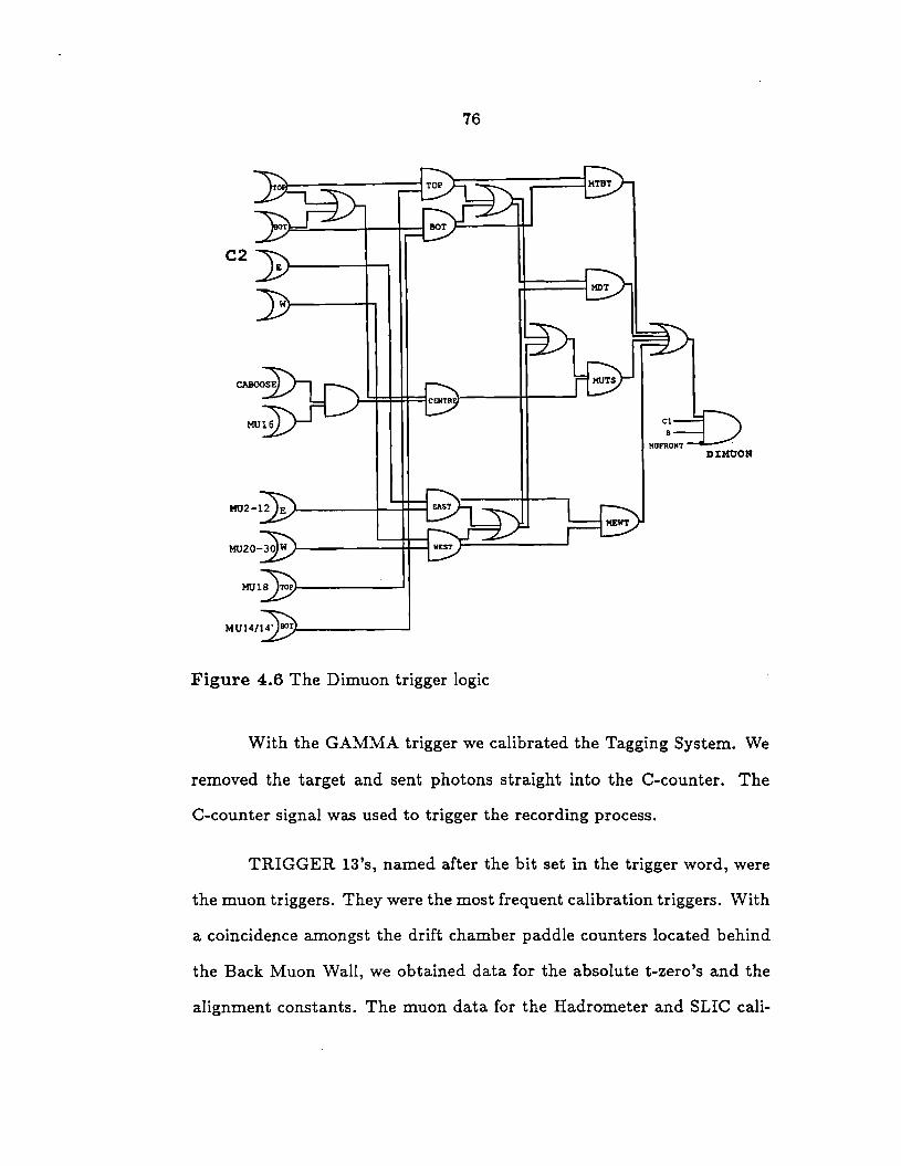
76
C2
DIMtJON
Figure 4.6 The Dimuon trigger logic
With the GAMMA trigger we calibrated the Tagging System. We
removed the target and sent photons straight into the C-counter. The
C-counter signal was used to trigger the recording process.
TRIGGER 13's, named after the bit set in the trigger word, were
the muon triggers. They were the most frequent calibration triggers. With
a coincidence amongst the drift chamber paddle counters located behind
the Back Muon Wall, we obtained data for the absolute t-zero's and the
alignment constants. The muon data for the Hadrometer and SLIC cali-
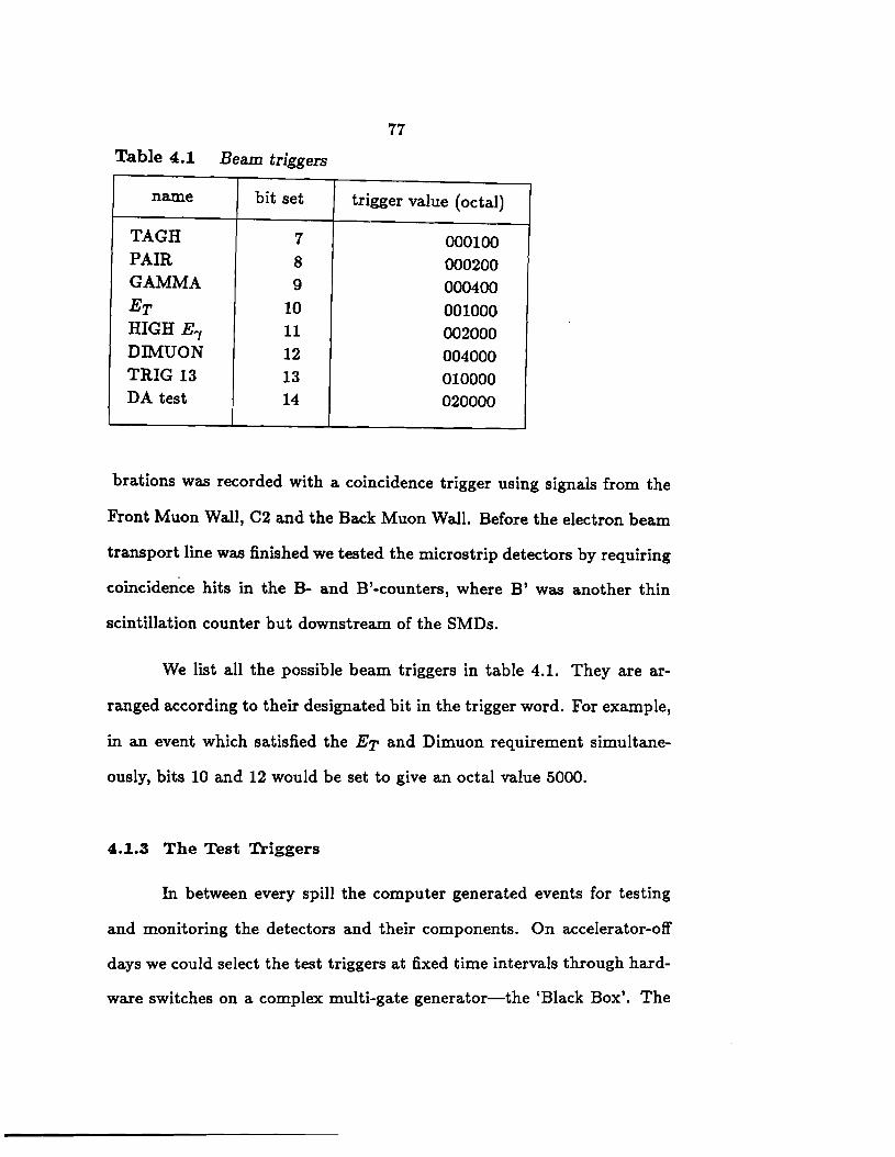
77
Table 4.1 Beam triggers
name bit set trigger value (octal)
TAGH 7 000100 PAIR 8 000200 GAMMA 9 000400 ET 10 001000 HIGH E"'f 11 002000 DIMUON 12 004000 TRIG 13 13 010000 DA test 14 020000
brations was recorded with a coincidence trigger using signals from the
Front Muon Wall, C2 and the Back Muon Wall. Before the electron beam
transport line was finished we tested the microstrip detectors by requiring
coinciden.ce hits in the B- and B'-counters, where B' was another thin
scintillation counter but downstream of the SMDs.
We list all the possible beam triggers in table 4.1. They are ar-
ranged according to their designated bit in the trigger word. For example,
in an event which satisfied the ET and Dimuon requirement simultane-
ously, bits 10 and 12 would be set to give an octal value 5000.
4.1.3 The Test Triggers
In between every spill the computer generated events for testing
and monitoring the detectors and their components. On accelerator-off
days we could select the test triggers at fixed time intervals through hard
ware switches on a complex multi-gate generator-the 'Black Box'. The
78
important inter-spill triggers are described below.
For the Downstream Laser events we pulsed a nitrogen laser. The
laser beam was transmitted by optical fibers to the phototubes in the
SLIC, the Hadrometer and the Cerenkov counters. A diode signal trig
gered the read-out and recording process. The high voltages for the pho
totubes were supplied by computer controlled LRS 4032 power supplies.
The voltage reading process was initiated by the High Voltage strobe. We
monitored the drift chamber high voltages, the fields of the analyzing mag
nets with Hall probes and the microstrip voltages on LRS 2232 ADC's.
The data for these ADC's was contained in the Low Voltage events. For
the Begin Spill events we gated the 2280 ADC's eight times before the spill,
averaged the pedestal values and sent the results back to the 2280 pro
cessors for internal subtraction. The Pedestal Subtracted Pedestals were
then checked to confirm that they were zero plus or minus a few counts
to allow for noise. At the beginning of every run we generated External
Autotrim triggers which were used to compute relative t-zero's. As for
the 2280 pedestals, the relative t-zero's were then fed back into the TDC
memory for internal subtraction.
4.2 The Data Acquisition
The data acquisition (DA) is the link between the hardware and
the software, between the spectrometer and the reconstruction/physics
analysis. The DA collects the digitized data for an event from the elec
tronics modules and formats the information into records that are written
79
to tape.
We used a PDP-11/55 to gather the data. Two Jorway 411 CA
MAC branch drivers interfaced the computer with the electronics, and a
Bison Interrupt Box provided a connection to the triggers. Im.mediately
after a trigger was received by the PDP, it initiated the digitization of
the ADC's, TDC's, etc., and raised a Busy level which vetoed all other
incomming triggers. Upon completion of the data transfers from the CA
MAC modules into a 128k bulk memory buffer the Busy was dropped and
a Clear issued. The Clear signal reset the modules and prepared them for
the next event.
The data in the bulk memory was formatted into -16k records, 6
to 8 events. One event was typically 2000 16-bit words long with about
1000 words for the fixed length data, mainly latches and ADC's, and with
the remainder composed of variable length data-TDC's, Scanners, etc ..
The event records were written to tape at 6250 Bpi. Because only -64
events could be stored in memory we had to continuously record on tape.
The maximum rate for data reading and writing was a little over 100
events/second with less than 30% dead-time. To achieve this rate we had
to place the different devices on the PDP Unibus in proper relation to
each other. The final configuration is illustrated in figure 4. 7. It proved
to be very important to locate the magtape controller close to the CPU
before the Jorways. With that arrangement we gained a factor of 2 in
tape writing speed; because with the Jorways close to the CPU they used
most of the CPU cycles and never allowed data transfers to tape.
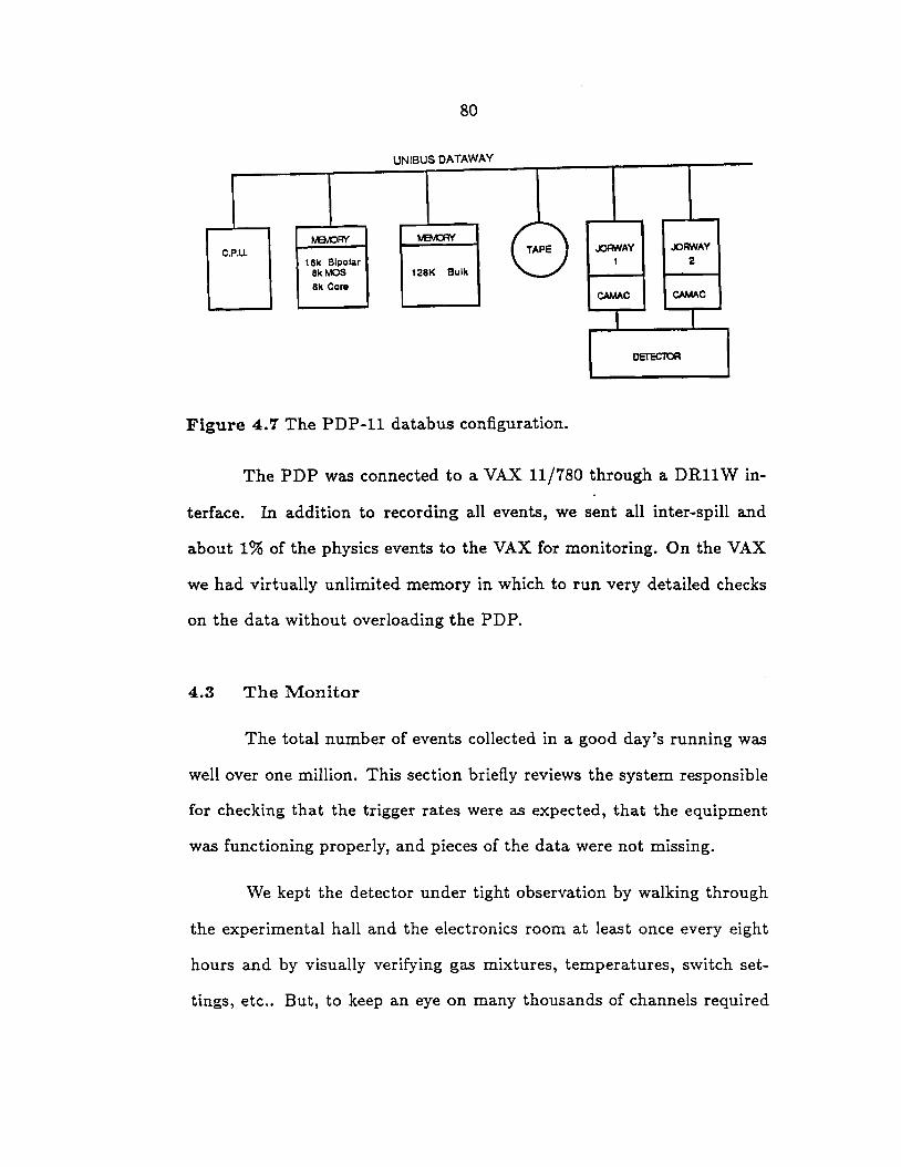
C.P.U 16k Bipolar
8kMOS 8k Core
80
UNIBUS OATAWAY
TAPE
128K Bulk
Figure 4. 7 The PDP-11 databus configuration.
.xJFfNAY 1
CAMAC
.xJFmAY 2
CAMAC
I I
DETECTOR
The PDP was connected to a VAX 11/780 through a DRll Win-
terface. In addition to recording all events, we sent all inter-spill and
about 13 of the physics events to the VAX for monitoring. On the VAX
we had virtually unlimited memory in which to run very detailed checks
on the data without overloading the PDP.
4.3 The Monitor
The total number of events collected in a good day's running was
well over one million. This section briefly reviews the system responsible
for checking that the trigger rates were as expected, that the equipment
was functioning properly, and pieces of the data were not missing.
We kept the detector under tight observation by walking through
the experimental hall and the electronics room at least once every eight
hours and by visually verifying gas mixtures, temperatures, switch set-
tings, etc .. But, to keep an eye on many thousands of channels required
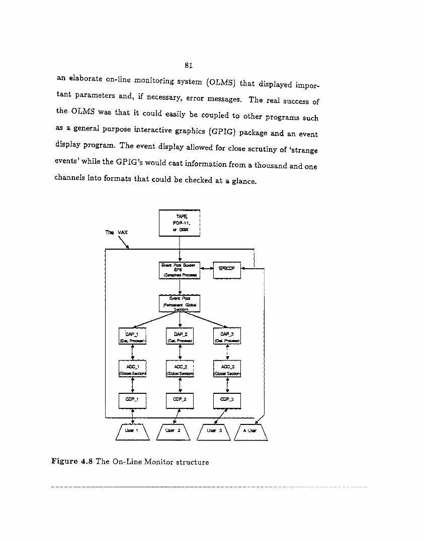
81
an elaborate on-line monitoring system (OLMS) that displayed impor-
tant parameters and, if necessary, error messages. The real success of
the. OLMS was that it could easily be coupled to other programs such
as a general purpose interactive graphics {GPIG) package and an event
display program. The event display allowed for close scrutiny of 'strange
events' while the GPIG's would cast information from a thousand and one
channels into formats that could be checked at a glance.
The VAX
TAPE POP·11, OI ClSK
Figure 4.8 The On-Line Monitor structure
82
The software 0 LMS structure is shown in figure 4 .8. The arrows
in the diagram indicate the direction of information flow. The input to
the OLMS was selected by the user to come from either disk, tape or
the PDP-11/DRll W link. The link was used during the data recording
periods, while disk and tape event sources were useful when the accelerator
was off. An event pool builder (EPB) transfered data from the devices
into a large storage array, the event pool. Detached analysis programs
{DAP), named thus because the user never communicated directly with
these programs, accessed the events in the pool and subjected them to
particular tests. While the DAP's were crunching away or waiting for
more events of a certain category the EPB threw out events which had
not been accesed for some time and added new events to the pool. The
CDP's, short for Control and Display Program, interacted with the DAP's
through a shared global common, the badly named ADC (Analyzed Data
Common). The ADC allowed for data and commands to be transferred
into and out of the DAP. Once a DAP was executing the user could exit
from the CDP to free the terminal for other projects and/or to check on
other DAP's.
At any one point during the data collection at least ten DAP's were
busy checking events. Each DAP performed analysis specific to a detec
tor system and was written by the respective experts. For example, the
2280ADC program monitored the 2280 ADC system and the associated
calorimetry by a) comparing pedestal counts and widths with milestone
values, b) by verifying the success of the pedestal subtraction, and c) by
83
checking the responses of the SLIC and Hadrometer phototubes to the
laser pulses. Other DAPs' checked Pairplane and Cerenkov pedestals,
laser signals, high voltages for the -600 phototubes, driftchamber and
SMD hits, Tagging System gains, data block presence and structure, Muon
Wall hit distributions, etc. The most important information was shown
on a dedicated graphics screen. The Scalar DAP displayed beam intensi
ties, B-counter, TAGH, ET, and other trigger rates, computer dead time,
number of drift chamber stops, etc .. Another screen was used to show the
alarm flags which were set by DAP's when a monitored variable or groups
of variables had moved out of bounds.
One of the highlights of the 0 LMS was the event display program.
Sections of the spectrometer could be displayed along with the hit patterns
and energy distributions. At the very beginning of the run, shortly after
we received our first photon beam, the event display was the first to
indicate that the triggers were picking up an unreasonably large number
of low energy events. The problem was fixed by raising the H threshold
to the previously mentioned value and by eliminating possible feedbacks.
Another display option used the GPIG's. They were designed for quick
exhibitions of participation plots, histograms and scatter plots. Typical
distributions for ET, H, B ... were kept on file and routinely compared
to t~e current ones.
84
5 The Reconstruction
The event reconstruction is divided into two segments, Passl and
Pass2. In Passl we reconstruct charged tracks from the raw microstrip
and drift chamber information. Pass2 has four parts: a short program es
timating the incident photon energy, a calorimeter reconstruction mainly
for neutral particle detection, a charged particle identification using the
Cerenkov data, and a vertexing program.
The two reconstruction programs initially ran on the Cyber sys
tem at FNAL. After the first test phase of the Advanced Computer Pro
gram (ACP) multiprocessor system [Na86] we transferred Passl, and later
Pass2, onto this microprocessor farm. With the latest 100 node version
we have reduced our reconstruction time/tape by a factor of 15-20.
5.1 Pass!
Two major subprograms, 81234 and SE8TR, handled the track re
construction and the momentum fits. 81234 found tracks in the region
covered by the SMD's and Dl, as illustrated in figure 5.1, and projected
them through the magnets into the other drift chambers (DC's). SESTR
supervised the DC reconstruction, matched DC hits with 81234 projec-
85
tions and picked up tracks from downstream vertices due to Ko 8
-+ ?r+ ?r
and A -+ p?r- decays. After all the tracks were found, Sl234 made a de
tailed momentum fit and eliminated low quality tracks.
We abandoned the usual method of first reconstructing tracks in
the region of least confusion behind the second magnet, and then project
ing them through the spectrometer, in favour of beginning the search in
the SMDs. The scheme of starting the tracking in the SMD's rather than
in D2 or D3 was much more advantageous for several reasons:
• Early reconstruction programs had shown that the DC's were only
~ 80% but the SMD's ~ 95% efficient. Part of the DC inefficien
cies were attributable to known efficiency holes in the important
central region [Es86]. The SMD 's had fewer noise hits to cause
confusion and no need to resolve left-right ambiguities because of
their intrinsically good resolution.
• The SMD reconstruction was considerably faster than the one for
the DC's, and in the end saved time for the DC tracking.
• The SMD /Dl combination with a total of 17 planes for 5 hits/view
had a much greater redundancy than any other connected field-free
region. Extrapolations of short track segments through the mag
nets, in order to pick up further hits, were laborious and imprecise.
• The forward extrapolation from the SMD /Dl region could be done
with more accuracy than the reverse. The projections into D2 or
D3 were good to within neighbouring cells while errors on projec-
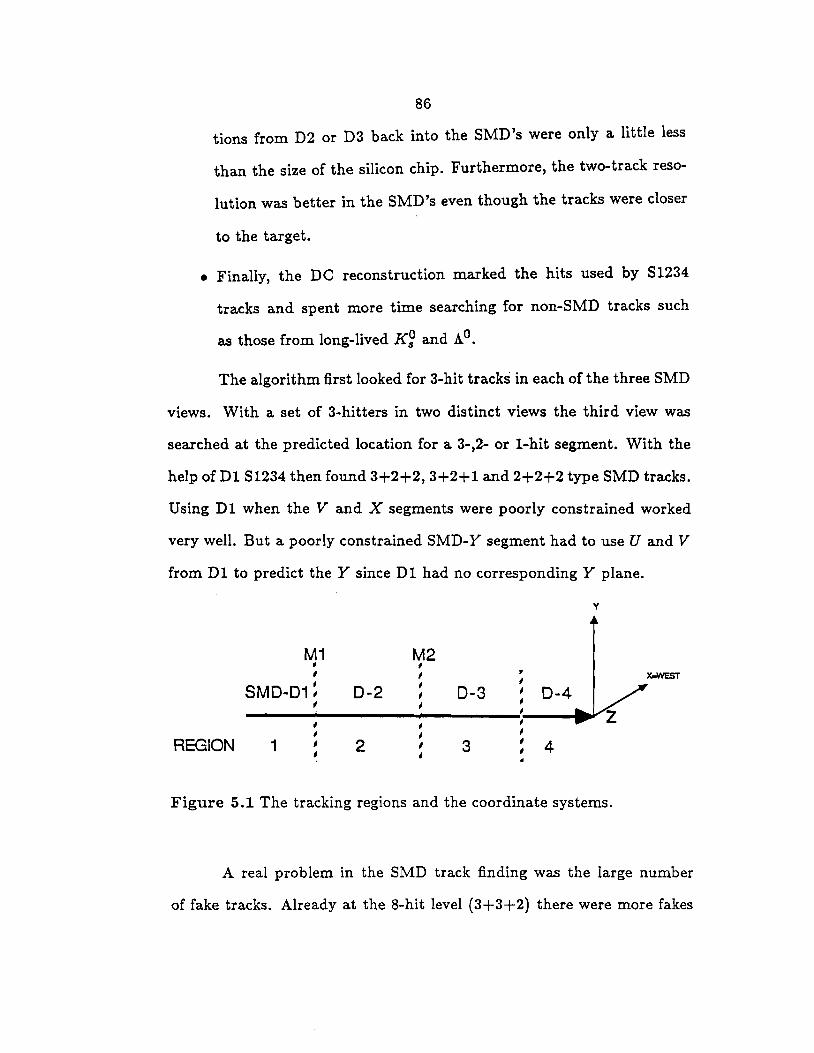
86
tions from D2 or D3 back into the SMD's were only a little less
than the size of the silicon chip. Furthermore, the two-track reso
lution was better in the SMD 's even though the tracks were closer
to the target.
• Finally, the DC reconstruction marked the hits used by 81234
tracks and spent more time searching for non-SMD tracks such
as those from long-lived K~ and A 0 •
The algorithm first looked for 3-hit tracks in each of the three SMD
views. With a set of 3-hitters in two distinct views the third view was
searched at the predicted location for a 3-,2- or 1-hit segment. With the
help of Dl 81234 then found 3+2+2, 3+2+1and2+2+2 type SMD tracks.
Using Dl when the V and X segments were poorly constrained worked
very well. But a poorly constrained SMD-Y segment had to use U and V
from D 1 to predict the Y since D 1 had no corresponding Y plane.
y
M1 M2 , , ' '
, ~WEST
' ' ' SMD-01' D-2 ' D-3 ' D-4 ' ' ' , , ' REGION 1 ' 2 3 4 '
Figure 5.1 The tracking regions and the coordinate systems.
A real problem in the SMD track finding was the large number
of fake tracks. Already at the 8-hit level (3+3+2) there were more fakes
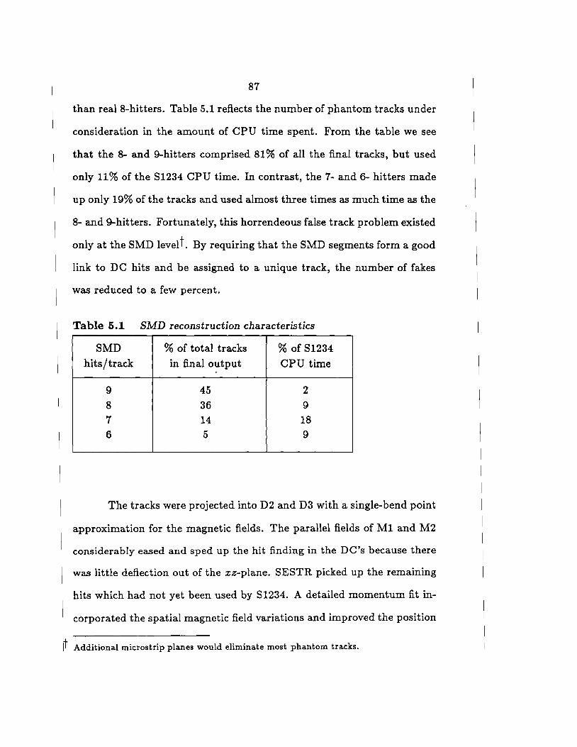
87
than real 8-hitters. Table 5.1 reflects the number of phantom tracks under
consideration in the amount of CPU time spent. From the table we see
that the 8- and 9-hitters comprised 81 % of all the final tracks, but used
only 11% of the 81234 CPU time. In contrast, the 7- and 6- hitters made
up only 19% of the tracks and used almost three times as much time as the
8- and 9-hitters. Fortunately, this horrendeous false track problem existed
only at the 8MD levelt. By requiring that the SMD segments form a good
link to DC hits and be assigned to a unique track, the number of fakes
was reduced to a few percent.
Table 5.1 SMD reconstruction characteristics
SMD % of total tracks % of 81234
hits/track in final output CPU time
9 45 2 8 36 9 7 14 18 6 5 9
The tracks were projected into D2 and D3 with a single-bend point
approximation for the magnetic fields. The parallel fields of Ml and M2
considerably eased and sped up the hit finding in the DC's because there
was little deflection out of the xz-plane. 8ESTR picked up the remaining
hits which had not yet been used by 81234. A detailed momentum fit in-
corporated the spatial magnetic field variations and improved the position
Additional microstrip planes would eliminate most phantom tracks.
88
1resolution by a factor of five. The fit was identical in form to Eq. (3.1),
but with QMDms non-zero and a function of the track coordinates.
The final Pass! output was appended to the raw data on a different
tape and included information pertaining to track quality, track parame
ters in each DC station region, charge and momenta of the particle.s. The
tracks were categorized by the flag JCATSG according to where hits were
found. A bit was set on for each chamber hit sequence. For example, a
track passing through the whole spectrometer would have JCATSG=15;
bit 1 set for SMD /Dl hits, bit 2 for D2, bit 3 for D3 and bit 4 for D4. Bit
5 was used to tag spurious tracks, e.g., tracks with poor chi-squares.
The total Cyber 175 CPU time used was ....... Q. 7 s for an ET event
and ....... i.o s for a. charm event. In a sample of charm events an average of
10 tracks were reconstructed of which 85% had hits in both SMD's and
DC's.
5.2 Pass2
In Pass2 the reconstruction processed the information from the
Tagging System, the Cerenkov counters and the calorimeters. A vertex
ing package combined SMD tracks into candidate primary and secondary
vertices.
The Tagging System reconstruction correlated the electron shower
energies and positions, and produced a best estimate for the incident pho
ton energy. The program flagged multi-electron buckets and/or possible
multiple interactions in the tungsten radiator.
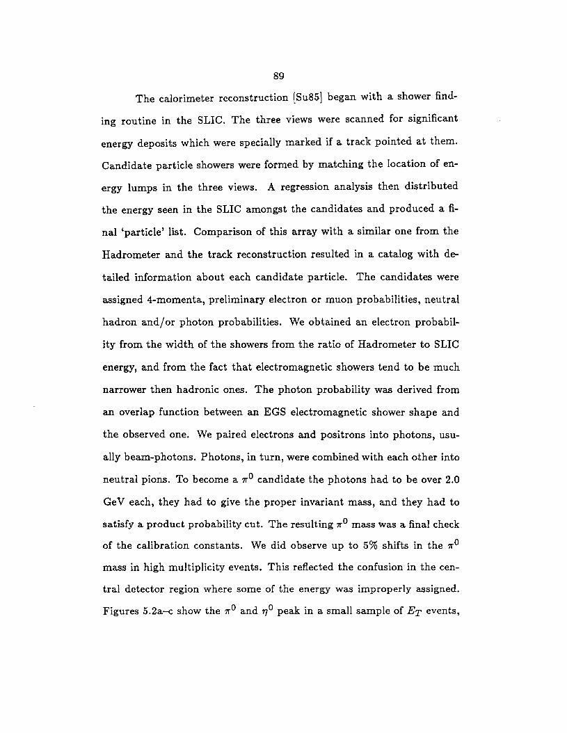
89
The calorimeter reconstruction [Su85] began with a shower find
ing routine in the SLIC. The three views were scanned for significant
energy deposits which were specially marked if a track pointed at them.
Candidate particle showers were formed by matching the location of en
ergy lumps in the three views. A regression analysis then distributed
the energy seen in the SLIC amongst the candidates and produced a fi
nal 'particle' list. Comparison of this array with a similar one from the
Hadrometer and the track reconstruction resulted in a catalog with de
tailed information about each candidate particle. The candidates were
assigned 4-momenta, preliminary electron or muon probabilities, neutral
hadron and/or photon probabilities. We obtained an electron probabil
ity from the width of the showers from the ratio of Hadrometer to SLIC
energy, and from the fact that electromagnetic showers tend to be much
narrower then hadronic ones. The photon probability was derived from
an overlap function between an EGS electromagnetic shower shape and
the observed one. We paired electrons and positrons into photons, usu
ally beam-photons. Photons, in turn, were combined with each other into
neutral pions. To become a 7ro candidate the photons had to be over 2.0
Ge V each, they had to give the proper invariant mass, and they had to
satisfy a product probability cut. The resulting 7ro mass was a final check
of the calibration constants. We did observe up to 5% shifts in the 7ro
mass in high multiplicity events. This reflected the confusion in the cen
tral detector region where some of the energy was improperly assigned.
Figures 5.2a-c show the 7ro and ,,., 0 peak in a small sample of ET events,
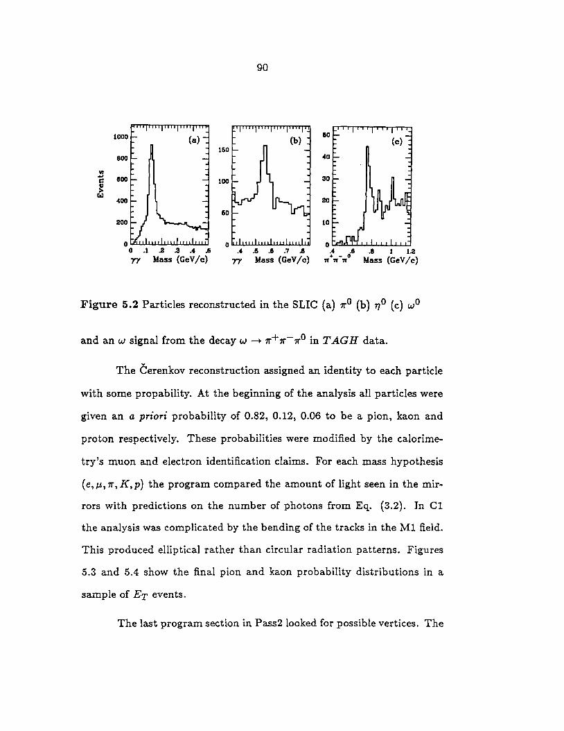
90
1000 60
160 800 .co
"' ..., 800 30 c: 100
~ rz.J
400 20
60 200 10
0 0 0 0 .1 .2 .3 ... .6 .4 .6 .e .7 .8 .4 .8 .8 1 1.2 Tl Mass (GeV /c) Tl Mass (GeV /c) + - 0 Mass (GeV /c) 7t 1T 11'
Figure 5.2 Particles reconstructed in the SLIC (a) 1r'o (b) TJO (c) wo
and an w signal from the decay w ~ 1r'+ 1r'-1r'O in TAG H data.
The Cerenkov reconstruction assigned an identity to each particle
with some propability. At the beginning of the analysis all particles were
given an a priori probability of 0.82, 0.12, 0.06 to be a pion, kaon and
proton respectively. These probabilities were modified by the calorime-
try's muon and electron identification claims. For each mass hypothesis
( e, µ, 1r', K, p) the program compared the amount of light seen in the mir
rors with predictions on the number of photons from Eq. (3.2). In Cl
the analysis was complicated by the bending of the tracks in the Ml field.
This produced elliptical rather than circular radiation patterns. Figures
5.3 and 5.4 show the final pion and kaon probability distributions in a
sample of ET events.
The last program section in Pa.ss2 looked for possible vertices. The
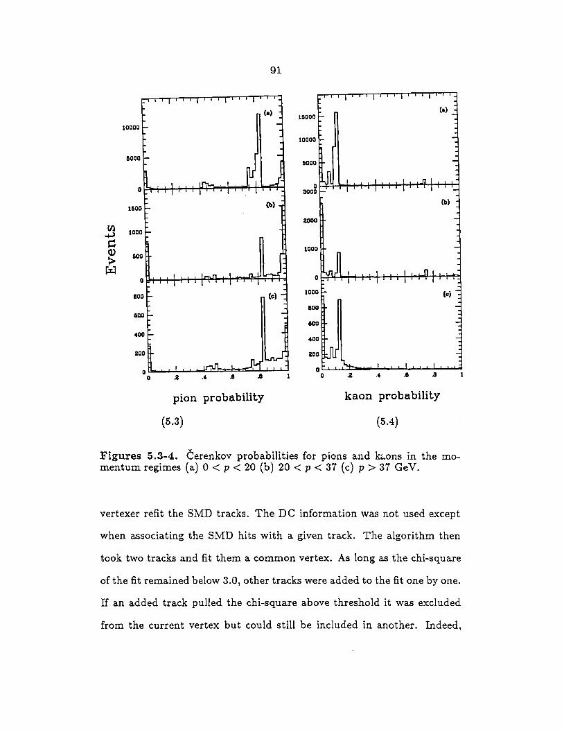
91
pion probability kaon probability
(5.3) (5.4)
Figures 5.3-4. Cerenkov probabilities for pions and kc...ons in the momentum regimes (a) 0 < p < 20 (b) 20 < p < 37 (c) p > 37 GeV.
vertexer refit the SMD tracks. The DC information was not used except
when associating the SMD hits with a given track. The algorithm then
took two tracks and fit them a common vertex. As long as the chi-square
of the fit remained below 3.0, other tracks were added to the fit one by one.
If an added track pulled the chi-square above threshold it was excluded
from the current vertex but could still be included in another. Indeed,
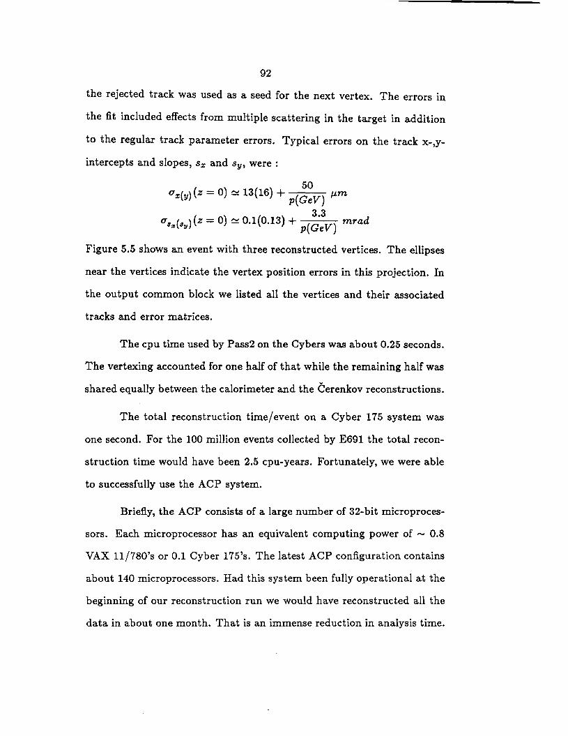
92
the rejected track was used as a seed for the next vertex. The errors in
the fit included effects from multiple scattering in the target in addition
to the regular track parameter errors. Typical errors on the track x-,y-
intercepts and slopes, Sx and sy, were :
50 D"x(y) (z = 0) ~ 13(16) + p(GeV) µm
u•.(•y) (z = 0) ~ 0.1(0.13) + p( ~:V) mrad
Figure 5.5 shows an event with three reconstructed vertices. The ellipses
near the vertices indicate the vertex position errors in this projection. In
the output common block we listed all the vertices and their associated
tracks and error matrices.
The cpu time used by Pass2 on the Cybers was about 0.25 seconds.
The vertexing accounted for one half of that while the remaining half was
shared equally between the calorimeter and the Cerenkov reconstructions.
The total reconstruction time/event on a Cyber 175 system was
one second. For the 100 million events collected by E691 the total recon-
struction time would have been 2.5 cpu-years. Fortunately, we were able
to successfully use the ACP system.
Briefly, the ACP consists of a large number of 32-bit microproces-
sors. Each microprocessor has an equivalent computing power of,...., 0.8
VAX 11/780's or 0.1Cyber175's. The latest ACP configuration contains
about 140 microprocessors. Had this system been fully operational at the
beginning of our reconstruction run we would have reconstructed all the
data in about one month. That is an immense reduction in analysis time.
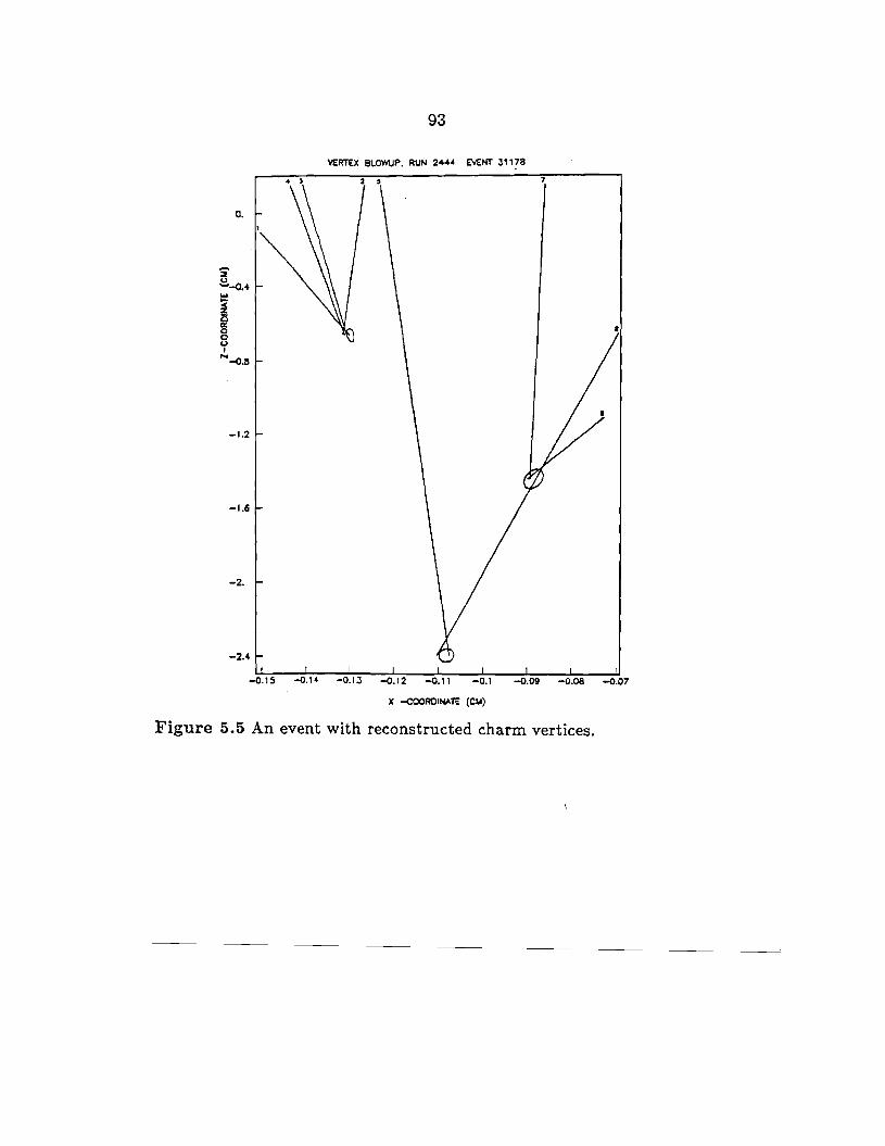
0.
2 (.)
--0.4 w
~ ~ 0 0 () I
..... -0.8
-1.2
-1.6
-2.
-2.4
93
VERTEX BLOWUP, RUN 24~ EV(NT 31178
-0.15 -0.14 -0.13 -0.12 -o., 1 -0.1 -0.09 -o.oa -0.01
X -<:OOROINATE (CM)
Figure 5.5 An event with reconstructed charm vertices.
94
6 The Data Analysis
We have analyzed part of the E691 data for the three charmed
mesons t no, n+ and nt and have extracted their lifetimes [An87a,b].
Because our neutral particle reconstruction efficiency was fairly low, and
because we had to start with at least two charged tracks to form secondary
vertices, we used only then decays with all charged particles in the final
state. For the n° we used three independent decay channels, n•+ --+
n°1r+ with no --+ K-1r+ or K-1r+1r-1r+, and n° --+ K-1r+ excluding
the n•+ events. In the n+ analysis we took events consistent with the
K- 'lr+ 'Tr+ decay. For the nt measurements we isolated the two modes
n+ --+ ...J.O'lr+ with ...J.O --+ K+ K- and f(•O K+ where f(•O --+ K-1r+ s 'I' ' 'I' ' ' •
In the following we describe the cuts, in particular the few vertex cuts
which dramatically reduced the backgrounds and allowed us to extract
large clean signals for the lifetime analysis presented in the next chapter.
6.1 The Data Reduction
After Pass2, the data was sent through several stripping programs.
The strips reduced the data to a manageable level with a high probabil-
t Anti-particles a.nd/or charge conjugates are implied unless stated otherwise
95
ity of charm in the surviving events. Thus, for the final analysis pro
grams the data inputs could all be stored on one or two disc files. The
strips increased the signal density in the selected decay channels by de
manding good quality tracks, good particle identifications and that the
reconstructed invariant masses lay within a predefined wide window. A
substripping program used the vertex information to reduce the back
grounds by a factor of about 50. Throughout the reduction and final
signal extraction, we never widened cuts once they were set in a previous
strip.
We required that the number of degrees of freedom (DOF) in the
track fit to the hits be larger than 11.5 and/or that the x2 of the track's
fit was less than 8.0. The DOF and x2 cuts eliminated a large fraction
of spurious tracks where a small number of hits had accidentally lined
up. The largest possible DOF was 39, 44 planes less 5 track parameters.
A cut on the allowed track categories, 3::; JC AT SG ::;15, ins.ured that
the particles at least passed through Cl. In addition, this cut threw out
a large number of low momentum tracks that were easily confused with
electrons. For some modes, we added an explicit low momentum cut. We
imposed a lower bound on the Cerenkov product probability for the final
state particle combination as, for example, in the decay n° ~ K-11"+ we
asked that CPROB2(K) x CPROB2(1r) ~ 0.2. Thus, there was always
at least one particle above its a priori probability assignment. Finally, the
particles had to make the proper charge combination before their invariant
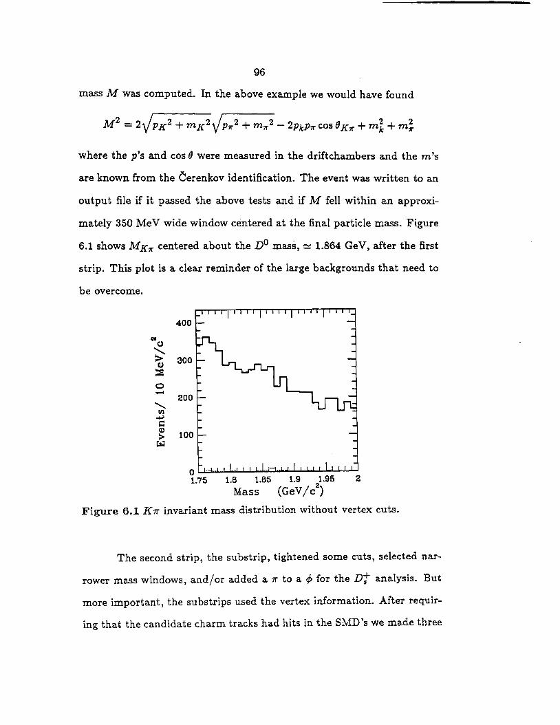
96
mass M was computed. In the above example we would have found
where the p's and cos fJ were measured in the driftchambers and the m's
are known from the Cerenkov identification. The event was written to an
output file if it passed the above tests and if M fell within an approxi
mately 350 Me V wide window centered at the final particle mass. Figure
6.1 shows MK tr centered about the Do mass, ~ 1.864 Ge V, after the first
strip. This plot is a clear reminder of the large backgrounds that need to
be overcome.
400
300
200
100
1.8 1.85
Mass 1.9 1.95
2 (GeV /c)
2
Figure 6.1 K 7r invariant mass distribution without vertex cuts.
The second strip, the substrip, tightened some cuts, selected nar
rower mass windows, and/ or added a 7r to a </> for the D"'[ analysis. But
more important, the substrips used the vertex information. After requir
ing that the candidate charm tracks had hits in the SMD's we made three
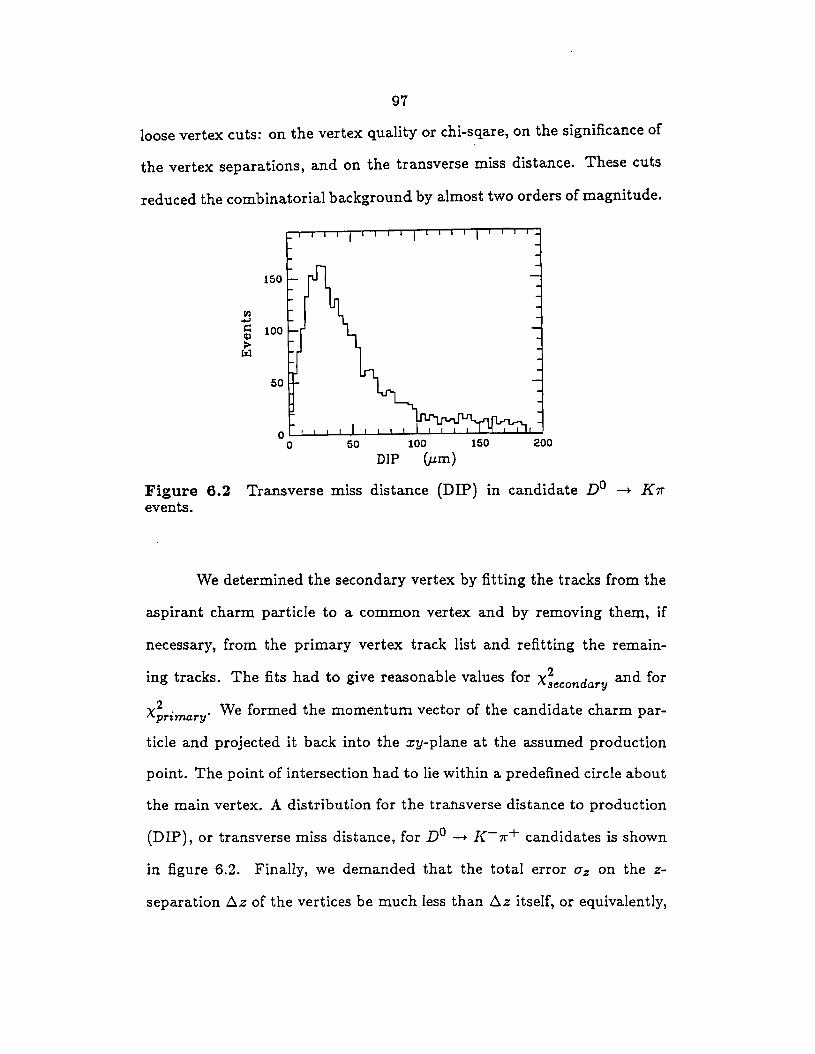
97
loose vertex cuts: on the vertex quality or chi-sqare, on the significance of
the vertex separations, and on the transverse miss distance. These cuts
reduced the combinatorial background by almost two orders of magnitude.
150
50
50 100 150 200
DIP (µm)
Figure 6.2 Transverse miss distance (DIP) m candidate n° ~ K 7r
events.
We determined the secondary vertex by fitting the tracks from the
aspirant charm particle to a common vertex and by removing them, if
necessary, from the primary vertex track list and refitting the remain
ing tracks. The fits had to give reasonable values for x2 d and for secon ary
X~rimary· We formed the momentum vector of the candidate charm par-
ticle and projected it back into the xy-plane at the assumed production
point. The point of intersection had to lie within a predefined circle about
the main vertex. A distribution for the transverse distance to production
(DIP), or transverse miss distance, for n° --+- K-?T+ candidates is shown
in figure 6.2. Finally, we demanded that the total error Uz on the z-
separation /),.z of the vertices be much less than /),.z itself, or equivalently,
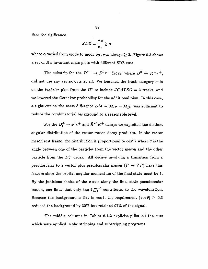
that the sigificance
98
~z SDZ = - ~a,
Uz
where a varied from mode to mode but was always~ 2. Figure 6.3 shows
a set of K 1r invariant mass plots with different SDZ cuts.
The substrip for the D*+ --+ D 07r+ decay, where no --+ K-1r+,
did not use any vertex cuts at all. We loosened the track category cuts
on the bachelor pion from the D* to include JCATSG = 3 tracks, and
we lowered the Cerenkov probability for the additional pion. In this case,
a tight cut on the mass difference ~M = MD• - M Do was sufficient to
reduce the combinatorial background to a reasonable level.
For the Dt --+ </Jo1r+ and f(*O K+ decays we exploited the distinct
angular distribution of the vector meson decay products. In the vector
meson rest frame, the distribution is proportional to cos2 (}where(} is the
angle between one of the particles from the vector meson and the other
particle from the D"J" decay. All decays involving a transition from a
pseudoscalar to a vector plus pseudoscalar meson (P --+ VP) have this
feature since the orbital angular momentum of the final state must be 1.
By the judicious choice of the z-axis along the final state pseudoscalar
meson, one finds that only the Yz~1o contributes to the wavefunction.
Because the background is fiat in cos 0, the requirement I cos OI 2::: 0.3
reduced the background by 30% but retained 97% of the signal.
The middle columns in Tables 6.1-2 explicitely list all the cuts
which were applied in the stripping and substripping programs.
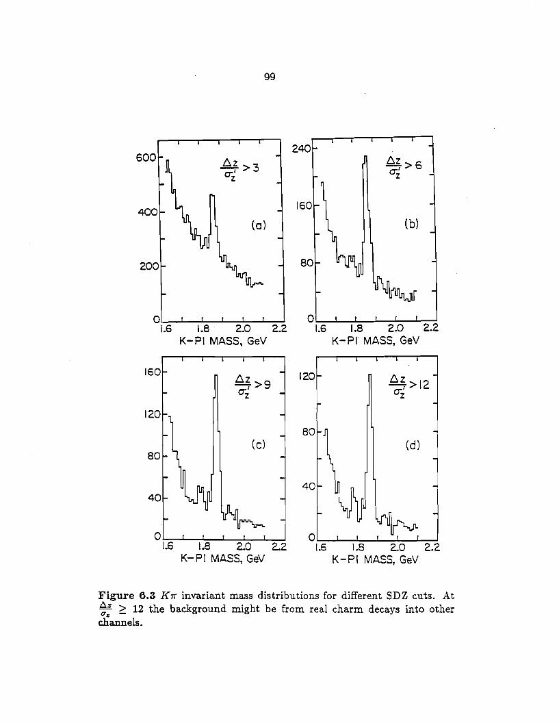
99
240 600
6.z >3 ~z >6 a:' a:' z z
400 (a) (b)
0 0 1.6 1.8. 2.0 2.2 1.6 1.8 2.0 2.2
K-Pl MASS, GeV K-Pr MASS, GeV
160 l:::.z >9 120
~z >12 a:' a:' z z
120
80 ( c) (d)
80
40 40
0--------~------~._~ 0.__----.~------~-----1.6 1.8 2.0 2.2 1.6 1.8 2.0 2.2
K-PI MASS, GeV K-PI MASS, GeV
Figure 6.3 K7r invariant mass distributions for different SDZ cuts. At ~: 2:: 12 the background might be from real charm decays into other channels.
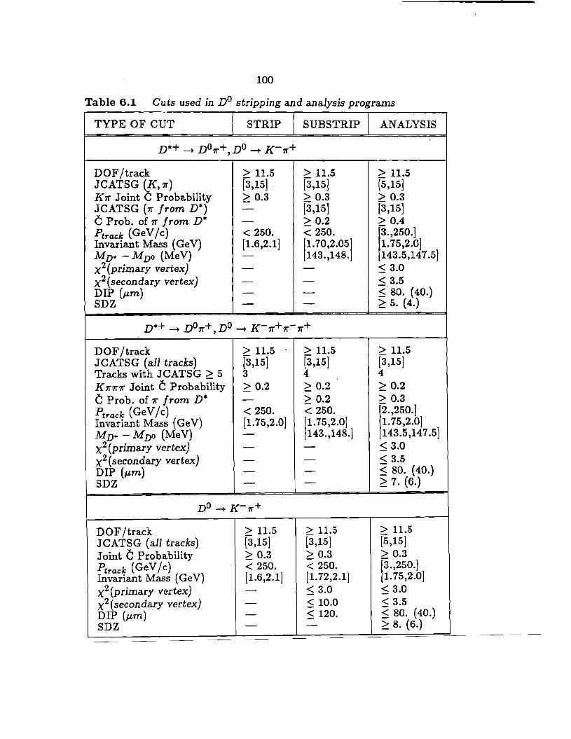
100
Table 6.1 Cuts used in n° stripping and analysis programs
TYPE OF CUT STRIP SUB STRIP ANALYSIS
n•+---+- n°1r+,n°-+ K-1r+
DOF /track > 11.5 > 11.5 > 11.5 JCATSG r' 7r) [3,15] [3,15] (5,15] K 7r Joint Probability ~ 0.3 > 0.3 > 0.3 JCATSG (7r from D*) - [3,15] [3,15) C Prob. of 7r from D* - ~ 0.2 > 0.4 Ptrack {GeV /c) < 250. < 250. 3.,250.] Invariant Mass (GeV) [1.6,2.1] 11. 70,2.051 1.75,2.0] MD· -Mno (MeV) - 143.,148. 143.5,147.5) x2(primary vertex} - - ~ 3.0 x2(secondary vertex) - - < 3.5 DIP (µm) - - ~- 80. (40.) SDZ - - 2 5. (4.)
n*+ -+ n°1r+ n° -+ K-'lr+'lr-'lr+ '
DOF/track > 11.5 > 11.5 > 11.5 JCATSG (all tracks) [3,15] [3,15] [3,15] Tracks with JCATSG > 5 3 4 4 K'lr'lr'lr Joint C Probabllity ~ 0.2 ~ 0.2 2 0.2 C Prob. of 'Ir from D* - ~ 0.2 > 0.3 Ptrack (GeV /c) < 250. < 250. 2.,250.) Invariant Mass (GeV) [1.75,2.0] 11.75,2.0] 1.75,2.0] Mn· -Mno (MeV) - 143.,148.] 143.5,147.5] x2 (primary vertex) - - ~ 3.0 x2(secondary vertex) - - < 3.5 DIP (µm) - - $ 80. ( 40.) SDZ - - ~ 7. (6.)
n°-+ K-'lr+
DOF/track > 11.5 > 11.5 > 11.5 JCATSG (all tracks) [3,15] [3,15] [5,15] Joint C Probability ~ 0.3 2 0.3 > 0.3 Ptrack (GeV /c) < 250. < 250. r-.250.] Invariant Mass (Ge V) [1.6,2.1] [l.72,2.1] 1. 75,2.0] x2 (primary vertex) - ~ 3.0 ~ 3.0 x2 (secondary vertex) - :::; 10.0 < 3.5 DIP (µm) - :::; 120. ~ 80. (40.) SDZ - - 2 8. (6.)
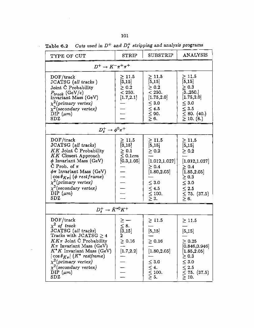
101
. Table 6.2 Cuts used in n+ and Dt stripping and analysis programs
TYPE OF CUT STRIP SUB STRIP ANALYSIS
n+ --+ K-1r+ 1r+
DOF/track > 11.5 > 11.5 > 11.5 JCATSG (all tracks) [3,15] [5,15] [5,15] Joint C Probability ~ 0.2 ~ 0.2 > 0.3 Ptrack (GeV /c) < 250. < 250. r-.250.] Invariant Mass (Ge V) [l.7,2.1] [1.75,2.0] 1.75,2.0] x2 (primary vertex) - ~ 3.0 ~ 3.0 x2 (secondary vertex) - :::; 4.5 < 3.5 DIP (µm) - :::; 90. ~ 80. (40.) SDZ - ~6. ~ 10. (8.)
Dt --+ </>o1r+
DOF/track > 11.5 > 11.5 > 11.5 JCATSG (all tracks) [3,15] [5,15] [5,15) KK Joint C Probability ~ 0.1 ~ 0.2 ~ 0.2 KK Closest Approach < O.lcm - -</> Invariant Mass (Ge V) [0.3,1.05] [l.012,1.027] [1.012,1.027] C Prob. of 'Jr - > 0.4 > 0.4 </>1r Invariant Mass (Ge V) - [i.80,2.05] [i.85,2.05] I cos 0 K?rl (</> rest frame) - - ~ 0.3 x2 (primary vertex) - ~ 3.0 :::; 3.0 x2 (secondary vertex) - ~ 4.5 :::; 2.5 DIP (µm) - ~ 100. ~ 75. (37.5) SDZ - ~ 3. ~ 6.
D+ --+ f(*O K+ s
DOF /track >- ~ 11.5 ~ 11.5 x2 of track < 8. - -JCATSG (all tracks) [3,15] [5,15] [5,15] Tracks with JCATSG > 4 2 - -KK'!r Joint C Probabillty ~ 0.16 ~ 0.16 > 0.25 K 'Jr Invariant Mass (Ge V) - - r-846,0.946] K* K Invariant Mass (Ge V) [l.7,2.2] [l.80,2.05] 1.85,2.05] I cos 0 K ?r I ( K* restframe) - - ~ 0.3 x2 (primary vertex) - :::; 3.0 :::; 3.0 x2 (secondary vertex) - :::; 4. < 2.5 DIP (µm) - :::; 100. ~ 75. (37.5) SDZ - ~ 5. ~ 10.
102
6.2 The Final Event Selection
We applied tighter cuts to the surviving events to produce a clean
and unbiased but still statistically significant charm sample. To avoid
decays behind the first SMD planes where the detection efficiency is poor,
we introduced one new cut that limited our decay volume to the region
upstream of the microstrips. The final set of cuts, except the fiducial cut,
are recorded in the last columns of tables 6.1-2.
About 20% of the events had a main vertex ambiguity. We resolved
it by reducing the DIP cut to half the previous value, to the number in
parenthesis in tables 6.1-2.. H the ambiguity still was not resolved, then
we chose the most downstream vertex as the production point. In events
with a n•+, the confusion was 75% of the time avoi~ed by demanding
that the bachelor pion track be included in the primary vertex track list.
We calculated the proper time t from a point Lmin = auz downstream of
the production vertex to the decay point,
t = ;tJ ( L - Lmin)' (1)
where /V = ~'and L was the primary and secondary vertex separation.
The method of starting the clock a fixed time into the decay had a simple
clear advantage: it made the proper time insensitive to the confusion
region around the primary vertex while preserving the exponential shape
of the lifetime distribution. Our time plots extend to about 4 lifetimes:
1.8 ps for the Do, 4.0 ps for then+, and 2.4 ps for the Dt.
We chose our fiducial volume to end at the first SMD plane, z1, to
103
avoid the region of partial detection and reconstruction efficiency beyond.
This imposed a definite upper limit ti, independent of the actual decay
point, on the proper time t
ti= 1~ ( zi - Zprimary) • (2)
This condition had almost no effect on the short lived D0 and D"t. The
target-SMD separation was large enough for most of them, l,99%, to decay
before the first plane. However, we lost about 35% of all D+'s, because
those produced at the downstream end of the target were not slow enough
to satisfy ti < 4.0ps. Rather than accept the loss of statistics we set a
less stringent limit and allowed events with ti < 2.0ps into the plot. This
introduced a bias against-inefficiency for-those events with lifetimes
greater than about 2 ps. We have calculated this inefficiency in two ways,
analytically and from the ti-distributions themselves. The details are
given in the appendix. Figures 6.4-6 are the invariant mass distributions
of the six modes as used for the lifetime measurement. We emphasize that
these signals were obtained with a small set of very simple cuts.
We used events from the wings of the mass distributions to esti
mate the background underneath the signals. The t-distributions for the
backgrounds were obtained in the same way as those for the signals, and
for the Dt we did not include the region around the Cabibbo suppressed
n+ decay. Table 6.3 summarizes some of the relevant information. There
we give the widths of the signal and wing regions, and the number of
events in each category.
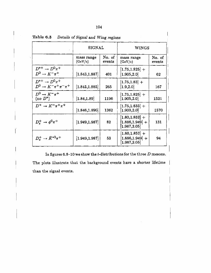
104
Table 6.3 Details of Signal and Wing regions
SIGNAL WINGS
mass range No. of mass range No. of (GeV /c) events (GeV /c) events
n•+-+ n°7r+ [1. 75,1.825] + n°-+ K-n+ [1.843,1.887] 401 [1.905,2.0] 62
n•+-+ D07r+ [l. 75,1.83] + n°-+ K-7r+1r-7r+ [1.845,1.885] 265 [l.9,2.0] 167
D0 -+ K-n+ 11. 75,1.825] + (no D*) [l.84,1.89] 1196 1.905,2.0] 1531
n+ -+ K...;.. 7r+ 7r+ 11. 75,1.833] + [1.846,1.890] 1362 1.903,2.0] 1570
[l.80,1.852] + Dt-+ </P1r+ (1.949,1.987] 82 f 1.886,1.949] + 131
1.987,2.05]
[l.80,1.852] + -Dt -+ K*o1r+ (1.949,1.987] 53 11.886,1.949] + 94
1.987 ,2.05]
In figures 6.8-10 we show the t-distributions for the three D mesons.
The plots illustrate that the background events have a shorter lifetime
than the signal events.
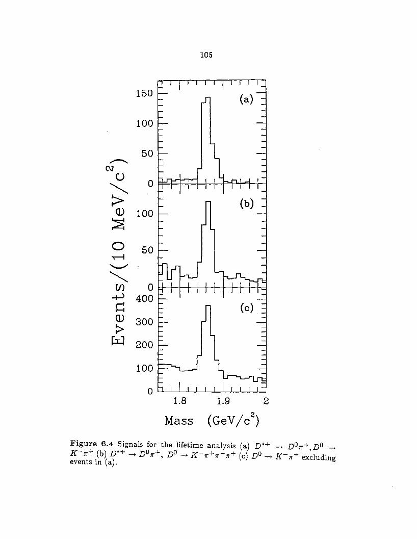
105
150
100
50 ~
C\2 ()
0
"" > (b) (]) 100
::g
0 50 ~
~
"" (/) 0 ~ 400 ~ (1) 300 > ~ 200
100
0 1.8 1.9 2
Mass 2
(GeV /c )
Figure 6.4 Signals for the lifetime analysis (a) D*+ -+ Do7r+, Do -+
K- rr+ (b) n*+ -+ n°7r+, n° -+ K- 7r+ 7r- 7r+ ( c) n° -+ K- 7r+ excluding events in (a).
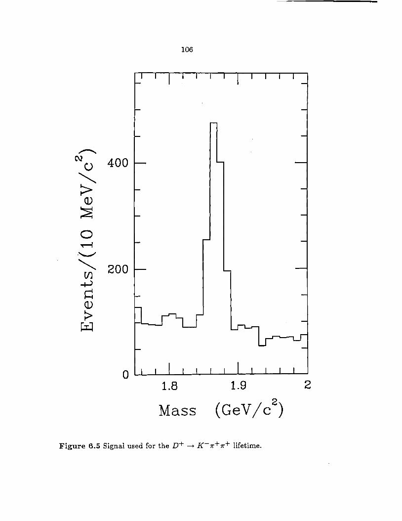
~
C\2 C)
"' > Q)
~
0 ~
·~
"' C/) ~
~ Cl)
:> t::il
400
200
106
1.8
Mass
1.9 2
(GeV /c )
Figure 6.5 Signal used for the n+ --+ K-1r+ Jr+ lifetime.
2
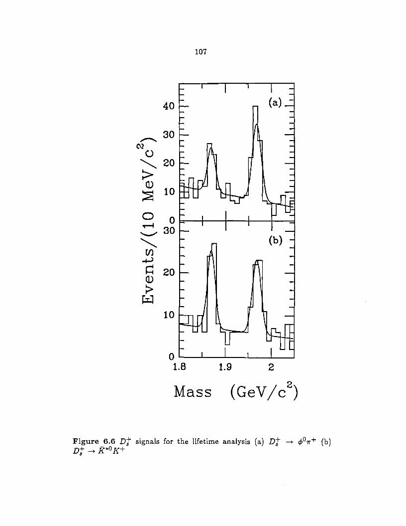
107
40
~ 30
C\2 ()
" 20
> Q) 10 ~
0 0 ~
'""---' 30
" (b)
{/) +)
~ 20 Q)
> ~
10
0 ----~-......_____, 1.8 1.9 2
Mass
Figure 6.6 Dt signals for the lifetime analysis (a) Dt --+ ¢07r+ (b) n+--+ K*°K+ s
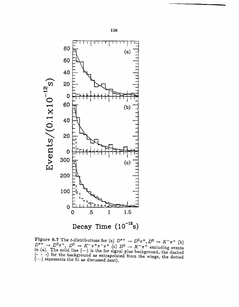
~
ti) C\1 .... I 0 ~
>< ~ . 0 '--"
" ti) ..._.)
~ Q)
> ~
80
60
40
20
0
60
40
20
0 300
108
( 10-125
) Decay Time
Figure 6.7 The t-distributions for (a) D*+ ~ n°7r+,n° ~ K-7r+ (b) D*+ ~ n°1r+, Do ~ K- 7r+ 7r- 7r+ ( c) n° ~ K- 7r+ excluding events in (a). The solid line (-) is the for signal plus background, the dashed (- - -) for the background as extrapolated from the wings, the dotted ( · · ·) rep res en ts the fit as discussed next) .
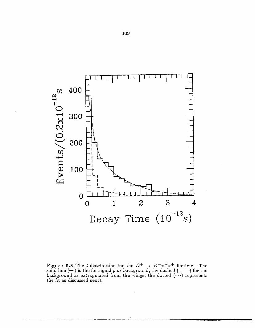
109
Vl 400 C\l
' \ .... I 0 \ ~ 300 ><
C\2 i . \ 0 \
"-" \
200 '
"" {/) .+-) \
~ Q) 100 > I
- 1
~ I
0 0 1 2
Decay Time
Figure 6.8 The t-distribution for the n+ ~ K-7r+1T"+ lifetime. The solid line (-) is the for signal plus background, the dashed (- - -) for the background as extrapolated from the wings, the dotted (· · ·) represents the fit as discussed next).
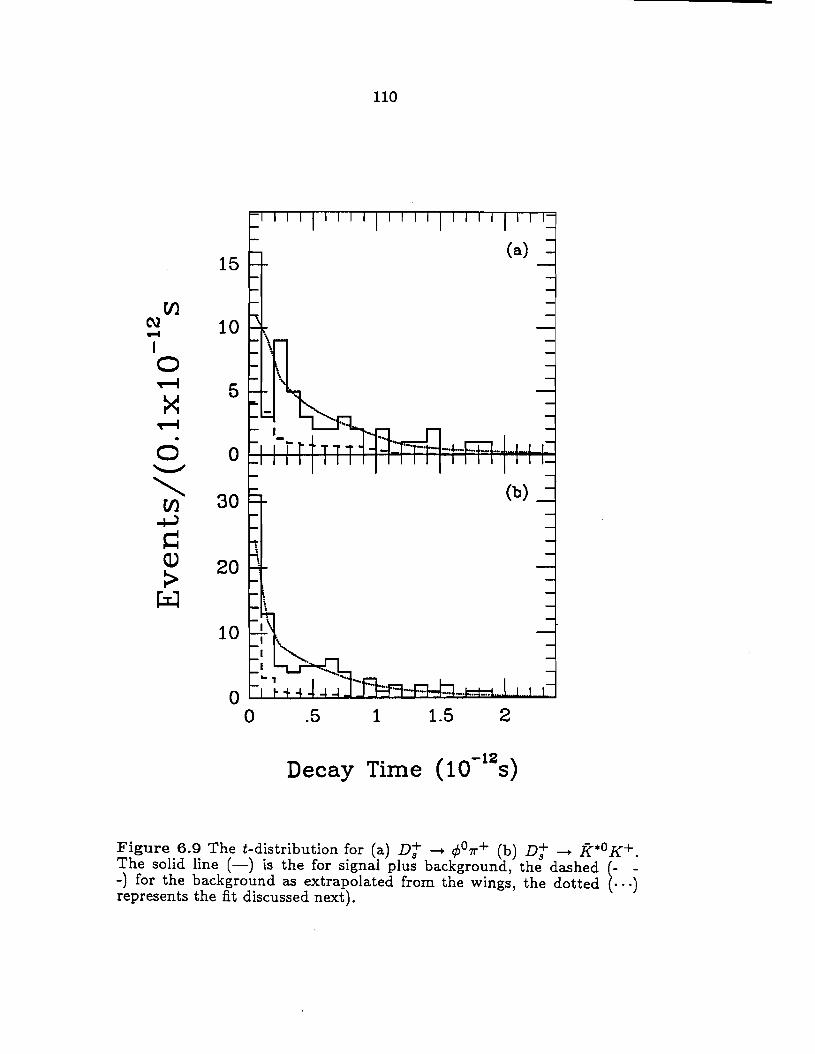
(/) C\J ..... I 0 -.-I
>< -.-I . 0 ..........,,,
" (/) +J ~ Cl)
> l::tJ
110
15 (a)
10 \
5
0
30
20
10
0 L...L~i..:i.::L:L.L.J.....c:::t.~::c:==a:~.....-~~
0 .5 1 1.5 2
( -12 ) Decay Time 10 s
Figure 6.9 The t-distribution for (a) Dt ---+ ¢07r+ (b) Dt ---+ f(*O K+. The solid line (-) is the for signal plus background, the dashed (- --) for the background as extrapolated from the wings, the dotted (· · ·) represents the fit discussed next).

111
7 The Lifetime Analysis
In the next few sections we give the details of our lifetime measure-
ments. We made a maximum likelihood fit to the observed time distribu-
tions to extract the lifetimes. From a Monte Carlo analysis we found that
deviations from the pure exponential behaviour of the time distributions
were small. Finally we discuss the sensitivity of the measurements to our
cuts, and we estimate our systematic errors.
7 .1 The Lifetime Fit
We fit the time distributions to a slightly modified exponential
plus the background distribution. The functional form for the number of
events at proper time t was
N(t) = N8 x l(t) x f(t) x
where
_i e .,.
+ B(t) (1)
B(t) was the background time distributions, obtained from events in
the wings of the invariant mass distributions and normalized to
the signal region.
f( t) was a Monte Carlo derived weight function that accounted for
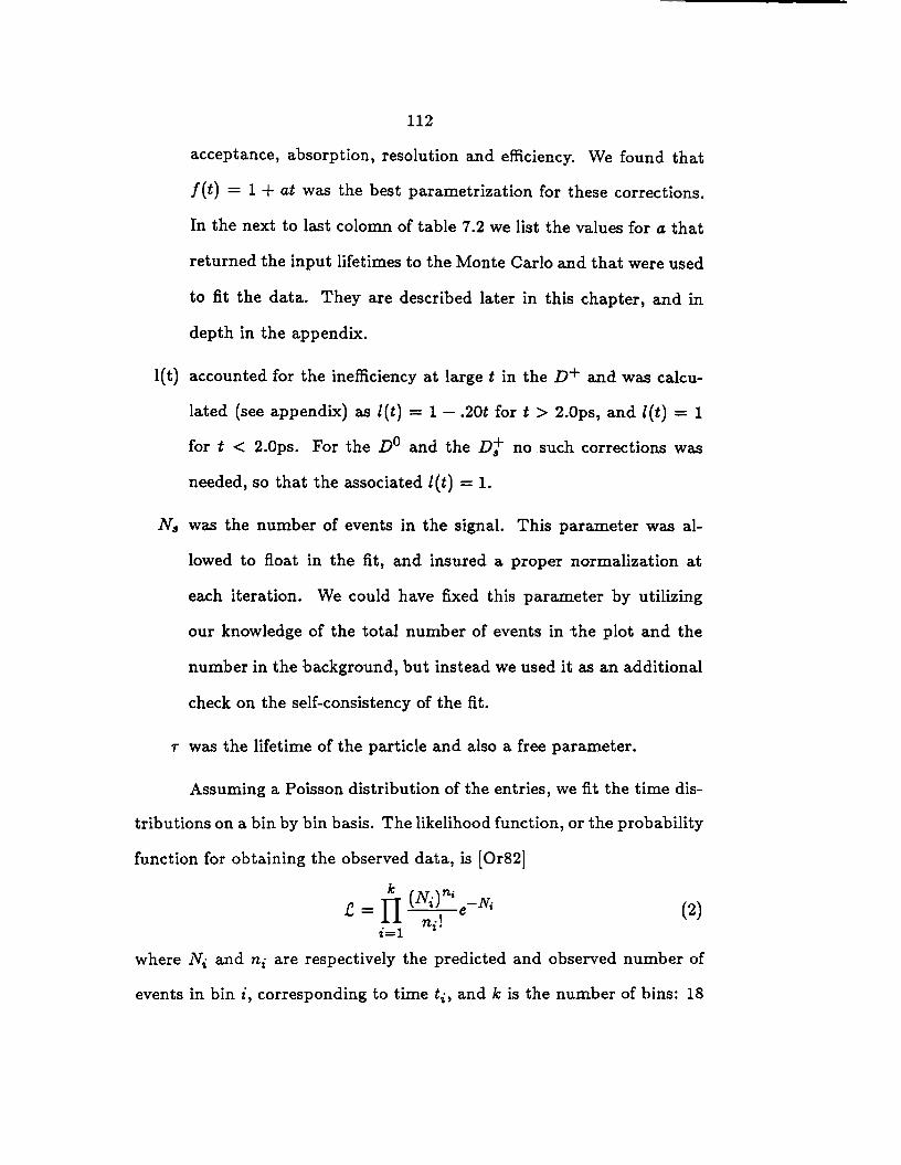
112
acceptance, absorption, resolution and efficiency. We found that
f(t) = 1 +at was the best parametrization for these corrections.
In the next to last colomn of table 7 .2 we list the values for a that
returned the input lifetimes to the Monte Carlo and that were used
to fit the data. They are described later in this chapter, and in
depth in the appendix.
l(t) accounted for the inefficiency at large t in the n+ and was calcu-
lated (see appendix) as l(t) = 1 - .20t for t > 2.0ps, and l(t) = 1
for t < 2.0ps. For the Do and the Dt no such corrections was
needed, so that the associated l(t) = 1.
Ns was the number of events in the signal. This parameter was al-
lowed to float in the fit, and insured a proper normalization at
each iteration. We could have fixed this parameter by utilizing
our knowledge of the total number of events in -the plot and the
number in the background, but instead we used it as an additional
check on the self-consistency of the fit.
r was the lifetime of the particle and also a free parameter.
Assuming a Poisson distribution of the entries, we fit the time dis
tributions on a bin by bin basis. The likelihood function, or the probability
function for obtaining the observed data, is (Or82]
(2)
where Ni and ni are respectively the predicted and observed number of
events in bin i, corresponding to time ti, and k is the number of bins: 18
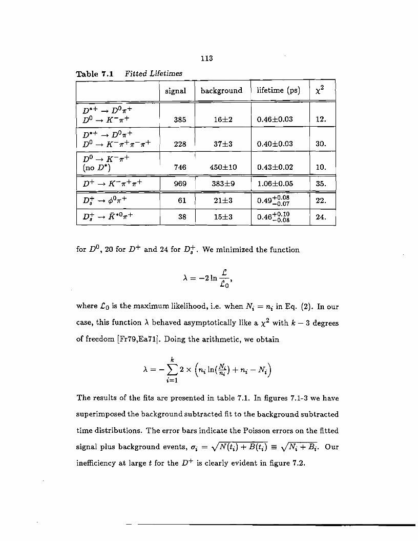
113
Table 7 .1 Fitted Lifetimes
signal background lifetime (ps) x2
D*+ ~ D01r+ n° ~ K-7r+ 385 16±2 0.46±0.03 12.
n•+ ~ n°1r+ n° ~ K-7r+1r-1r+ 228 37±3 0.40±0.03 30.
D0 ~ K-7r+ (non*) 746 450±10 0.43±0.02 10.
n+ ~ K-7r+1r+ 969 383±9 1.06±0.05 35.
nt ~ </>o1r+ 61 21±3 0 49+0.08 . -0.07 22.
n+ ~ f(•o'lr+ s 38 15±3 0 46+0·10 . -0.08 24.
for n°, 20 for n+ and 24 for nt. We minimized the functio~
where lo is the maximum likelihood, i.e. when Ni = ni in Eq. (2). In our
case, this function .X behaved asymptotically like a x2 with k - 3 degrees
of freedom [Fr79,Ea71]. Doing the arithmetic, we obtain
k
.X = - " 2 x (n · ln ( !fi) + n · - N·) L..J i ni i i
i=l
The results of the fits are presented in table 7.1. In figures 7.1-3 we have
superimposed the background subtracted fit to the background subtracted
time distributions. The error bars indicate the Poisson errors on the fitted
signal plus background events, ui = y'N(ti) + B(ti) = y'Ni +Bi. Our
inefficiency at large t for the n+ is clearly evident in figure 7.2.
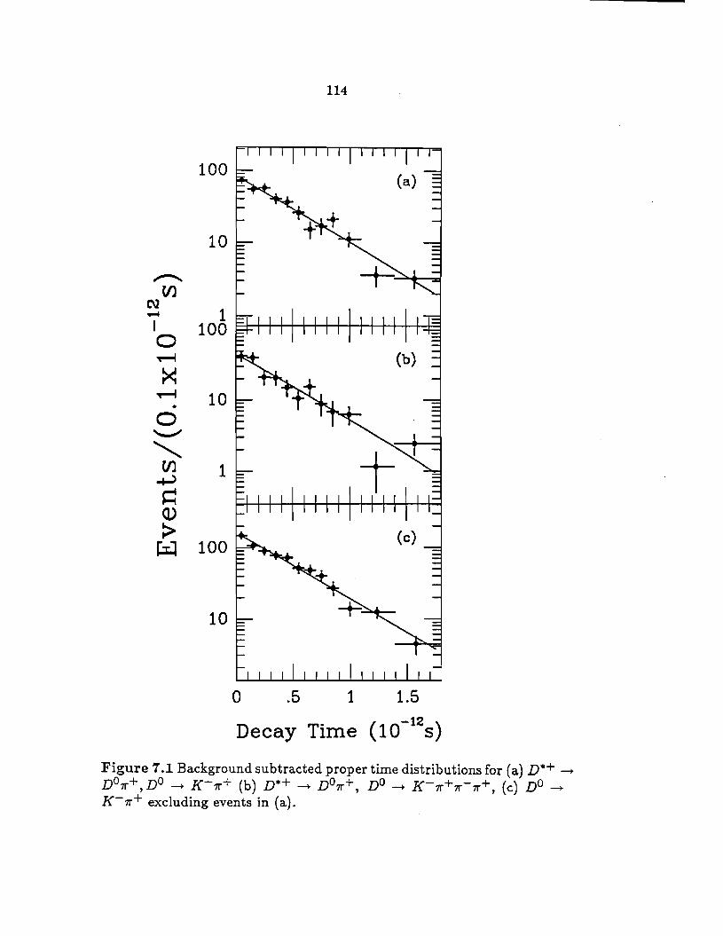
114
100
10
,,,,-...... Vl
C\2 1 ......
I 100 0 ,....-I
>< ,....-I 10 . 0 '--""
' Vl 1 ..,._)
~ Q)
> ~ 100
10
0 .5 1 1.5
Decay Time (10-12s)
Figure 7 .I Background subtracted proper time distributions for (a) D*+ ~ D0 1r+,no ~ K-7r+ (b) D*+ ~ D01r+, D0 ~ K-7r+7r-7r+, (c) n° ~ K-7r+ excluding events in (a).
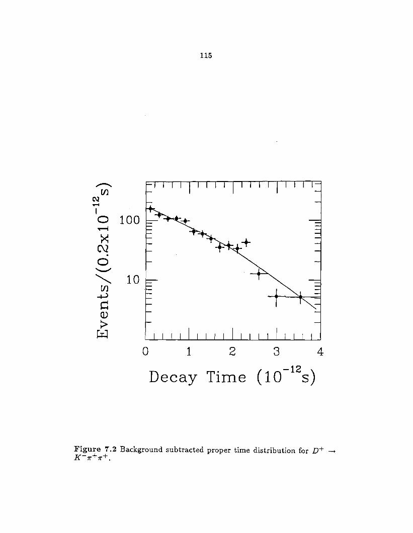
115
~
(/) t\2 ..... I 0 100 """'""" >< C\2 . 0 "---"'
" 10 [/)
+)
c: Q)
:> ~
0 1 2 4
Decay Time
Figure 7 .2 Background subtracted proper time distribution for n+ --+ K-7r+7r+.
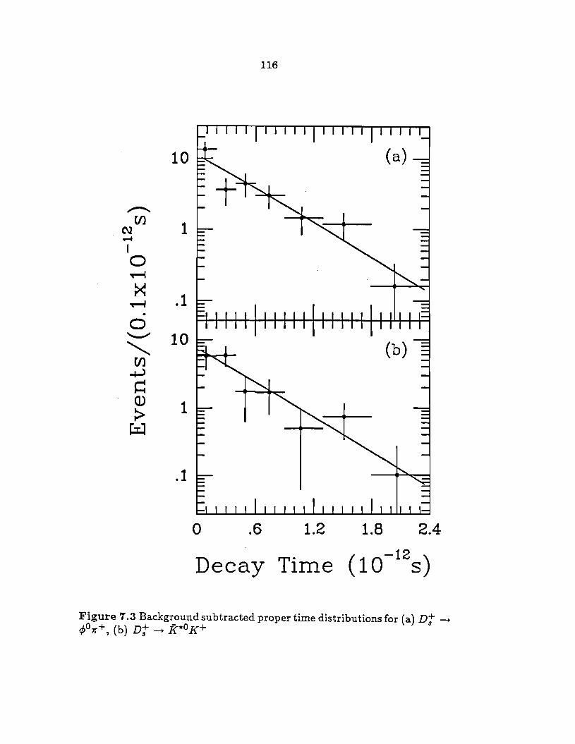
116
10
~
{/) 1 N ......
I 0 ~
>< .1 ~ . 0 ~ 10
' {/)
-+-> ~ Q) 1 >
J::t:l
.1
0 .6 1.2 1.8 2.4
Decay Time (10-12s)
Figure 7.3 Background subtracted proper time distributions for (a) Di ~ </Jo7r+' (b) nt ~ K*o K+
117
7.2 The Monte Carlo
In the Monte Carlo we simulated the spectrometer response to hy
pothetical charm events. Thus, we could 'calcula~e' the integrated effects
of the geometrical acceptances, the ineffi.ciences and other losses. We de
termined their combined impact on the lifetimes by comparing the Monte
Carlo generated lifetimes to the reconstructed ones.
The Monte Carlo generated charm according to the photon gluon
fusion model. We used the LUND model to hadronize the quark and gluon
fragments. From truth-tables containing information on 4-momenta, charge,
birth and death coordinates, mass, etc., we generated a tape identical to
the raw data tapes. The particles were traced through the spectrometer
and the detector responses were simulated. The simulations included all
the known inefficiences such as those in the centraf driftchamber region,
the electronic noise and cross talk, a distribution of background muons,
etc., and of course the geometrical acceptances of the detectors. The MC
used a set of stored EGS shower shapes to model the response of the SLIC
to electromagnetic showers. The energy from hadronic interactions in the
calorimeters was distributed according to a parametrization of the width
and depth of the showers. We included multiple scattering, secondary in
teractions and ~~ losses in the target, the B-counter, the SMD 's, etc .. The
events were reconstructed with the standard Passl and Pass2 programs.
We made detailed comparisons between the MC and the data for
SMD and drift chamber hit distributions, track resolutions, momentum
and mass distributions, etc., to insure that we had not introduced any
118
unrealistic biases. Considering that the mass resolutions compare within
a few percent to the ones in the data, and that the distributions shown in
figures 7.4a-f agree well, we are confident that this Monte Carlo is good
simulation of charm in the spectrometer.
For the lifetime analysis the theoretical details of the production
model were not important, especially since the distributions associated
with the SMD's agreed with the data. Figures 7.4c-f illustrate that the
number of vertices, the number of tracks per vertex, the DIP and the x2
distributions in the MC and the data are about equal.
From the Monte Carlo we extracted the a parameter in the correc-
. tion function. We made time distributions as for the data but let a vary in
the fit rather than r. For r we used the input Monte Carlo lifetimes: 0.45
ps, 1.10 ps and 0.40 or 0.50 ps for the n°, n+, and Dt, respectively. For
the Dt" we used two different input lifetimes to test the sensitivity of a.
The fact that we were able to explain the contributions to the corrections
within statistics gave us great confidence in our approach.
7 .3 The Corrections and the Error Analysis
From figures 7 .1-3 it is evident that the signal is almost a pure
exponential, a straight line on the semi-log plot. In fact, the corrections
we derived from the Monte Carlo reduced the lifetimes from the simple
exponential values by less than 12%. We studied the correction to the
exponential behavior in detail and accounted for most of it.
Table 7.2 contains a division of the slope a of the correction func-
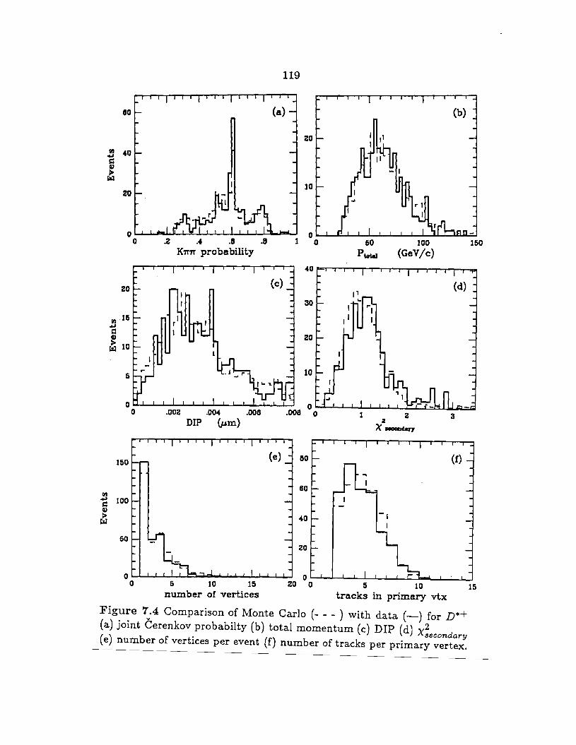
119
80 {a) (b)
20
'2 40 ...,, r:: Q)
> ~
10 20
0 0 .2 ·' .B .8 60 100
Knn probability p\ot.al {GeV/c)
40
20
30
112 15 .a
= u r!l 10
20
6 10
.002 .004 .008 .008 2 3 DIP {µm) z
X ROODduT
150 80
so rn ~ 100 = Q)
40 > ~
50 20
5 10 15 20 5 10 number of vertices tracks in primary vtx
Figure 7.4 Comparison of Monte Carlo (- - - ) with data (-) for D*+ {a) joint Cerenkov probabi!ty {b) total momentum (c) DIP (d) x;econdary
( e) number of vertices per event (f) number of tracks per primary vertex.
150
15
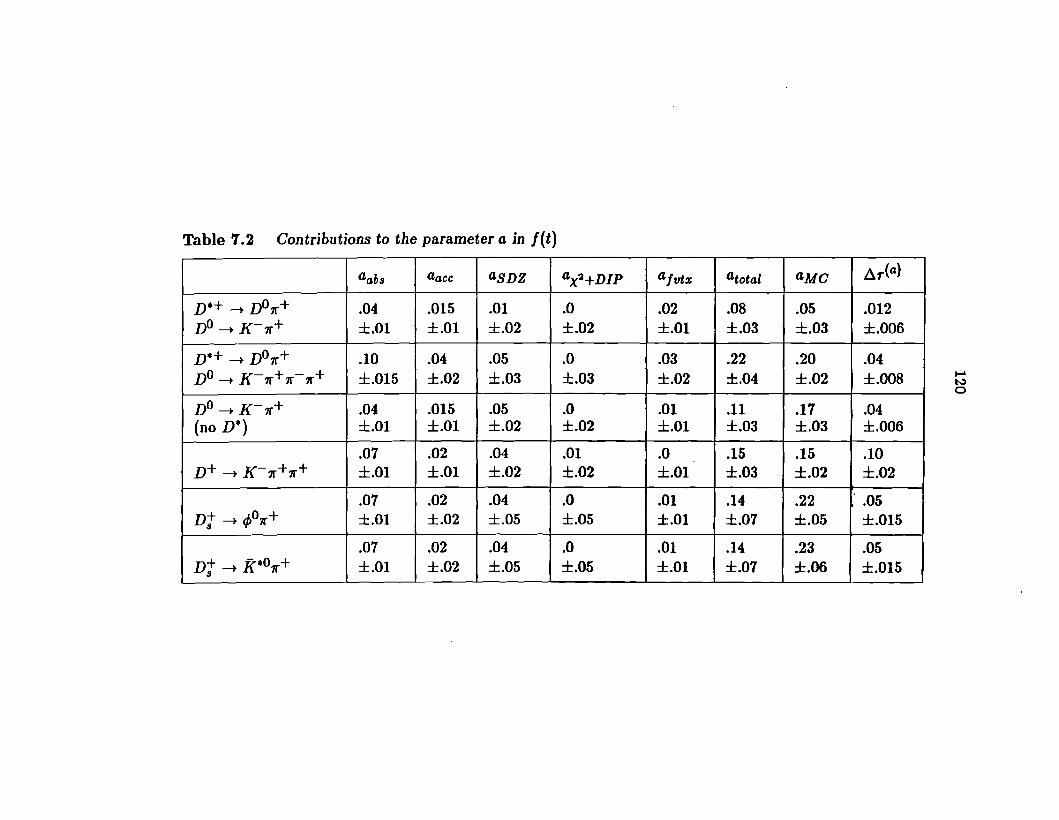
Table 7.2 Contributions to the parameter a in f(t)
a abs aacc as DZ 4x2+DIP a/vt:i atotal a Mc ~T(a)
n•+ --+ n°1r+ .04 .015 .01 .0 .02 .08 .05 .012 n° --+ K-n+ ±.01 ±.01 ±.02 ±.02 ±.01 ±.03 ±.03 ±.006
n•+ --+ n°1r+ .10 .04 .05 .0 .03 .22 .20 .04 n° --+ K-n+ 1r-1r+ ±.015 ±.02 ±.03 ±.03 ±.02 ±.04 ±.02 ±.008
n° --+ K-n + .04 .015 .05 .0 .01 .11 .17 .04 (no D*) ±.01 ±.01 ±.02 ±.02 ±.01 ±.03 ±.03 ±.006
.07 .02 .04 .01 .0 .15 .15 .10 n+ --+ K-n+'ff+ ±.01 ±.01 ±.02 ±.02 ±.01 ±.03 ±.02 ±.02
.07 .02 .04 .0 .01 .14 .22 : .05 Dl --+ <f,01r+ ±.01 ±.02 ±.05 ±.05 ±.01 ±.07 ±.05 ±.015
.07 .02 .04 .0 .01 .14 .23 .05 n+ --+ f(•O'lf +
s ±.01 ±.02 ±.05 ±.05 ±.01 ±.07 ±.06 ±.015
121
tion into its major components. The last two columns give. the slope as
obtained from the Monte Carlo and the corresponding shift in lifetime.
The contributions from absorption and acceptance, aabs and aacc, are
calculated analytically in the appendix and are listed in the second and
third columns. The next two columns, labelled by asnz and ax2+DIP'
give the contrihutions from our vertex cuts. They were studied by varying
the cuts in the Monte Carlo and in the data. By comparing the effects of
the cuts on the MC and the data we insured that they behaved alike, and
by refitting the MC lifetime distributions to obtain a new a, we gauged
our sensitivity to the different cuts and estimated their contribution to a.
The effects of resolution are implicitly included in asnz·
We also studied the problem of proper primary vertex selection in
our algorithms. A choice of false vertices much further upstream than
the true ones would have introduced a bias. Figure 7.5a is a plot of the
difference of the generated MC time and our reconstructed time without
the tmin shift. The r.m.s. width is 0.15 ps. In figure 7.5b we illustrate the
effect of the tmin offset. In distributions like 7.5b we counted the number
of events with tMc - t ~ 0 and found that < !% of the events without
the D* had tMc - t < 0 while for the D* s it was < 1!%. The lifetimes
of these events were larger by about 0.1 ps which caused a slight upward
shift in T approximately given by
~Tfvtx ~ Ntlyi~ X 0.1,
where N and Nfvtx are the total number of events and the number of
misverticized events respectively. The contributions to a due to vertex
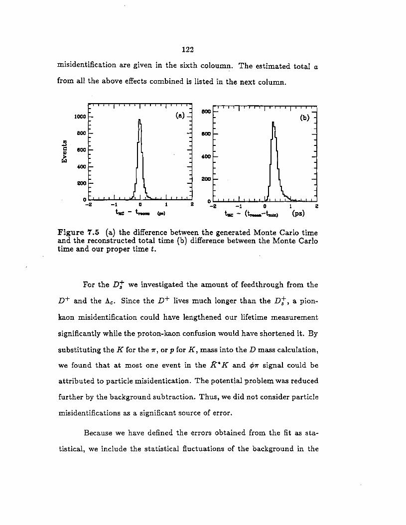
122
misidentification are given in the sixth coloum.n. The estimated total a
from all the above effects combined is listed in the next column.
800 1000
800 ISOO
rn ..,a . c 800 ~ •oo ~
400
200 200
-1 0 2 -1 0 1 2 txc - t.,.._ Cp.) t.c - (t.,_-t._.> (ps)
Figure 'T.5 (a) the difference between the generated Monte Carlo time and the reconstructed total time (b) difference between the Monte Carlo time and our proper time t.
For the Dt we investigated the amount of feedthrough from the
n+ and the Ac. Since the n+ lives much longer than the Dt, a pion
kaon misidentification could have lengthened our lifetime measurement
significantly while the proton-kaon confusion would have shortened it. By
substituting the K for the '1r, or p for K, mass into the D mass calculation,
we found that at most one event in the K* K and <P1r signal could be
attributed to particle misidentication. The potential problem was reduced
further by the background subtraction. Thus, we did not consider particle
mis identifications as a significant source of error.
Because we have defined the errors obtained from the fit as sta-
tistical, we include the statistical fluctuations of the background in the
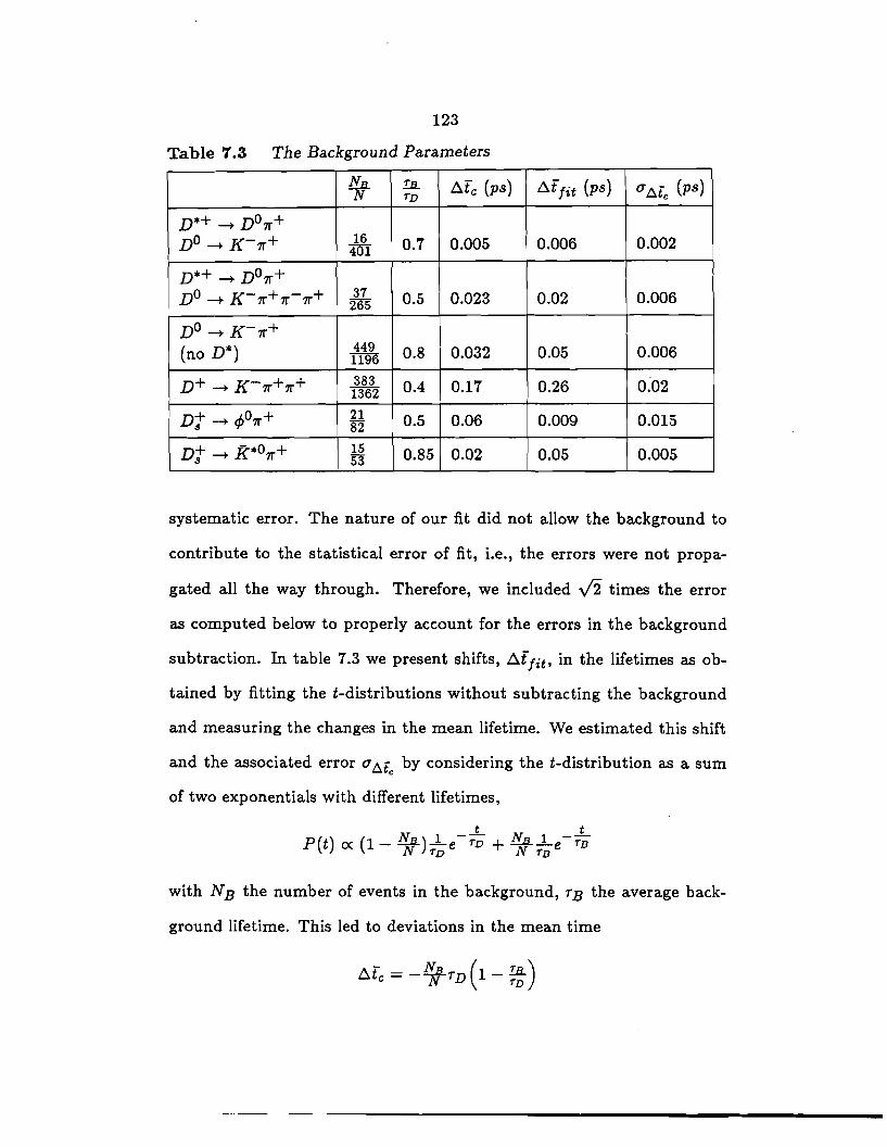
123
Table 7 .3 The Background Parameters
~ !Jl. Afc (ps) Af fit (ps) <7 Ate (ps) TD
D*+--+ D01r+ Do--+ K-1r+ 16 0.7 0.005 0.006 0.002 401
D*+--+ D01r+ D0 --+ K- 1r+ 7r- 7r+ 37 0.5 0.023 0.02 0.006 265
Do--+ K-1r+ (no D*) 449 0.8 0.032 0.05 0.006 1196
D+ --+ K-1r+1r+ 383 0.4 0.17 0.26 0.02 1362
Dt --+ </>o1r+ 21 0.5 0.06 0.009 0.015 82
n+ --+ K*o1r+ 15 0.85 0.02 0.05 0.005 8 53
systematic error. The nature of our fit did not allow the background to
contribute to the statistical error of fit, i.e., the errors were not propa-
gated all the way through. Therefore, we included V2 times the error
as computed below to properly account for the errors in the background
subtraction. In table 7.3 we present shifts, Af/it, in the lifetimes as ob
tained by fitting the t-distributions without subtracting the background
and measuring the changes in the mean lifetime. We estimated this shift
and the associated error a Ate by considering the t-distribution as a sum
of two exponentials with different lifetimes,
with NB the number of events in the background, TB the average back-
ground lifetime. This led to deviations in the mean time
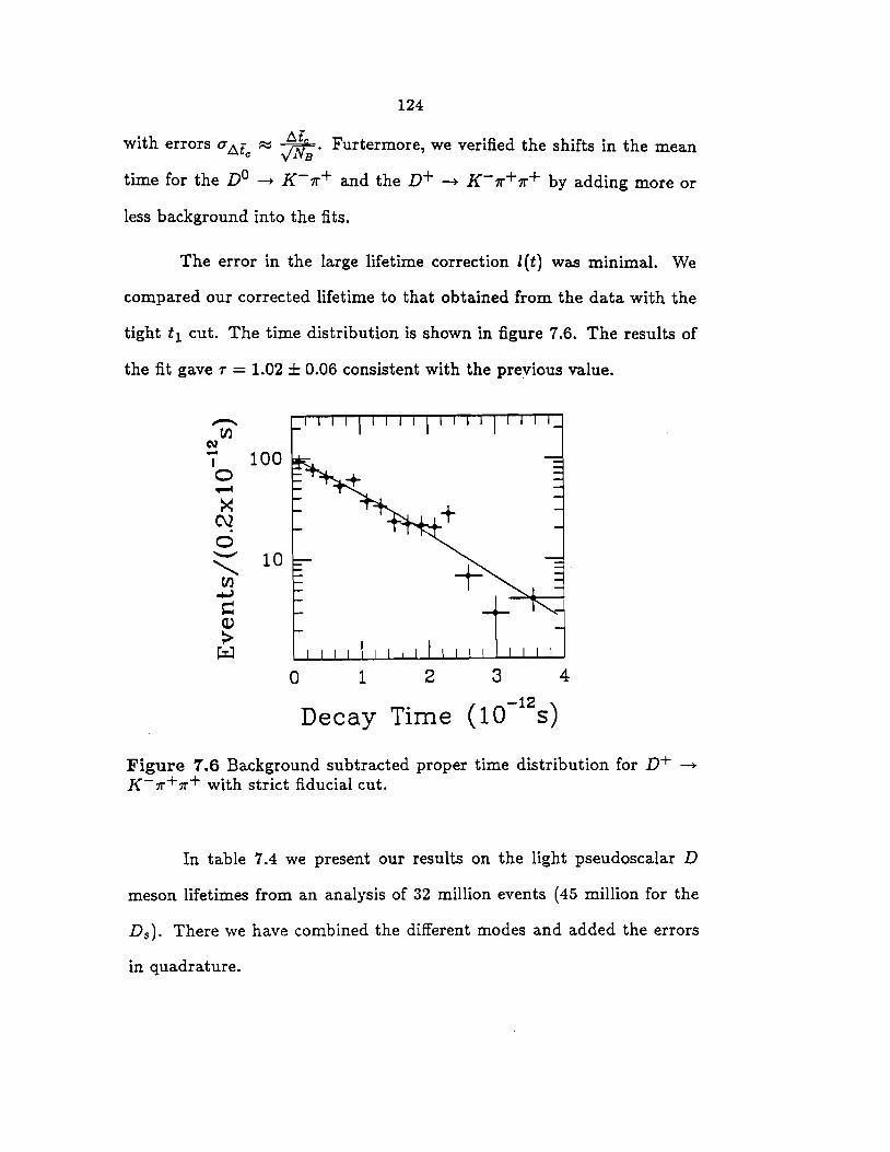
124
with errors O' Af c :::::: J/;;. Furtermore, we verified the shifts in ·the mean
time for the D0 -+- K-7r+ and the n+ -+- K-7r+7r+ by adding more or
less background into the fits.
The error in the large lifetime correction l ( t) was minimal. We
compared our corrected lifetime to that obtained from the data with the
tight t1 cut. The time distribution is shown in figure 7.6. The results of
the fit gave T = 1.02 ± 0.06 consistent with the preyious value.
100
10
0 1 2 3 4
Decay Time (10-12
s)
Figure 7 .6 Background subtracted proper time distribution for n+ -+
x-1r+ 1r+ with strict fiducial cut.
In table 7.4 we present our results on the light pseudoscalar D
meson lifetimes from an analysis of 32 million events ( 45 million for the
D5 ). There we have combined the different modes and added the errors
in quadrature.
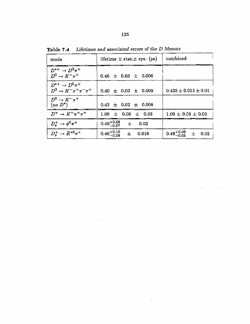
125
Table 7.4 Lifetimes and associated errors of the D Mesons
mode lifetime ± stat.± sys. (ps) combined
D*+ --+ D0 7r+ Do--+ K-7r+ 0.46 ± 0.03 ± 0.006
D*+ --+ D0 7r+ D0 --+ K-7r+7r-7r+ 0.40 ± 0.03 ± 0.009 0.435 ± 0.015 ± 0.01
D0 --+ K-7r+ (no D*) 0.43 ± 0.02 ± 0.008
D+ --+ K-7r+7r+ 1.06 ± 0.05 ± 0.03 1.06 ± 0.05 ± 0.03
Dt --+ </>o7r+ 0 49+0.08 . -0.07 ± 0.02
D+ --+ f(•O'lr+ 8
0 46+0.l0 . -0.08 ± 0.016 0 4g+0.06 . -0.05 ± 0.02
126
8 Synopsis
In this final chapter we briefly review the highlights of this exper
iment, E691, and summarize the lifetime results. We also compare our
results, when possible, with theoretical calculations. The thesis concludes
with a brief discussion of further possible areas of investigation.
The success of the experiment, E691, relative to past experiments
can be· attributed to several factors: a high resolution microstrip vertex
detector, a very efficient spectrometer, trigger and reconstruction, and
the better duty cycle of the Tevatron. With the microstrip detectors we
were able to resolve vertex longitudinal separations down to 400 microns.
This resolution was ideal for isolating the charm secondary from the pro
duction vertex because average charm decay lengths were about 4000 mi
crons. Our excellent resolving power allowed us to directly observe the
exponential nature of the decay. Improvements to the spectrometer and
the charged track reconstruction algorithm nearly doubled the number of
observed charm events. Increasing the number of drift chamber planes
for redundancy raised the per track detection efficiency by 10%. Finer
segmentation in the Cerenkov counters, and higher reflectivity mirrors
and Winston cones, more than doubled the number of detected photo-
127
electrons per track. Furthermore, we improved the momentum resolution
by increasing the magnetic fields. We increased the charm content of the
data by a factor of 2.5 through a large transverse energy trigger based
only on calorimeter information. We also benefited from the higher en-
ergies available at the Tevatron in addition to the longer spills. Because
of the larger proton energies we could extend the incident photon spec-
trum to 260 GeV. Finally, with the 20-fold increase in the spill length we
recorded many more events which would have otherwise been lost to dead
times. Thus, for the same amount of charm we had a significantly shorter
running time than previous experiments.
A partial analysis of our data has produced a large clean charm
sample. We have used this sample to measure the lifetimes of the three
pseudoscalar mesons. From a full reconstruction of 32 million events we
have obtained, with few and simple cuts, 969 n+'s decaying into the
K-1r+1r+ channel. We have reconstructed a total of 1360 n°'s in three
decay modes: Do -+ K-1r+, with and without the D*+ requirement, and
n•+-+ D01r+ where n°-+ K-1r+1r-1r+. An analysis of 45 million events
produced 99 Dt from the </>o1r+ and f(•O K+ decay modes combined. The
results of the lifetime analysis were
TDo =4.35 ±0.15 ±0.lOx 10-13s
TD+=l0.6 ±0.5 ±0.3 X 10⁻¹³s
tr - 4 8 +0.6 'Dt- · -0.5
where the errors are statistical and systematic respectively.
In table 8.1 we list all the previous lifetime measurements. In the
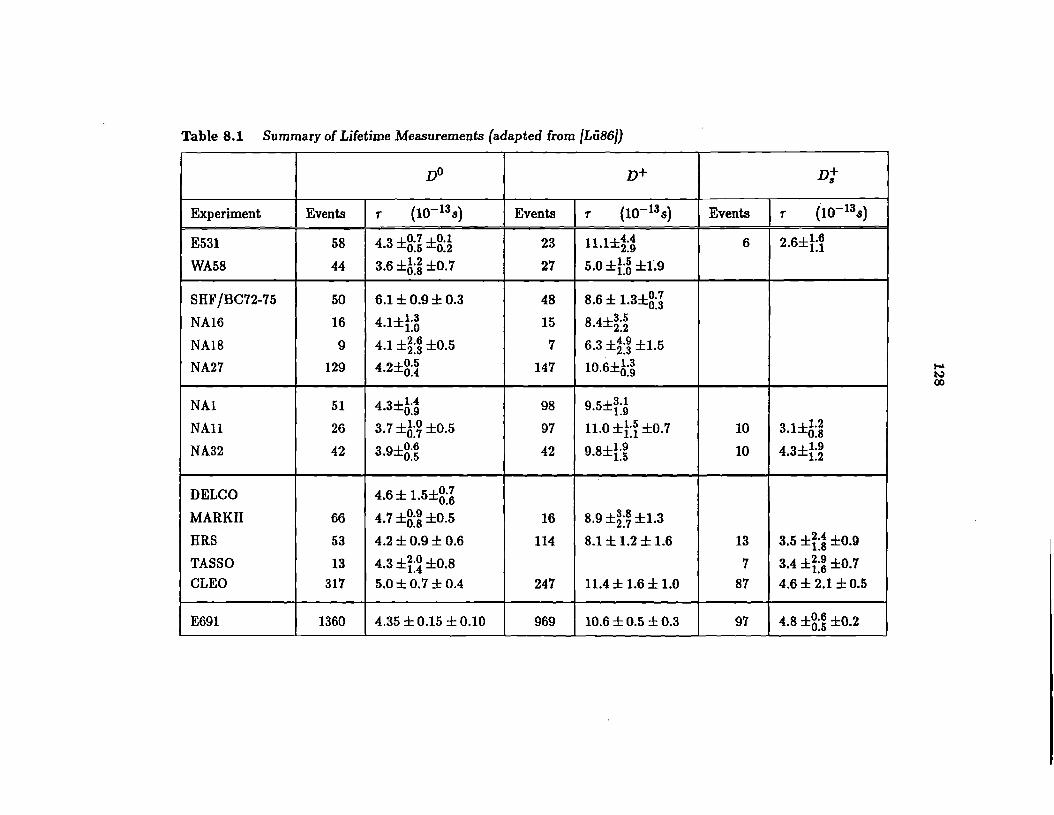
Table 8.1 Summary of Lifetime Measurements (adapted from [Lii86})
no v+ v+ s
Experiment Events f (10-13s) Events f (10-13 s) Events f (10-13s)
E531 58 4 3 ±0.7 ±0.1 . 0.5 0.2 23 11.1±~:a 6 2.6±H
WA58 44 3.6 ±A:i ±o. 1 27 15 . 5.0 ±1:0 ±1.9
SHF /BC72-75 50 6.1 ± 0.9 ± 0.3 48 8.6 ± 1.3±8:~
NA16 16 4.1±}:3 15 8.4±~:~ NA18 9 4.1 ±~:g ±0.5 7 6.3 ±~:~ ±1.5
NA27 129 4.2±8:~ 147 10.6±A:g
NAl 51 4.3±A:~ 98 9.5±f:~
NAll 26 s. 1 ±A:~ ±o.s 97 11.0±}j ±0.7 10 3.1±A:~
NA32 42 3.9±8:~ 42 9.8±}:g 10 4.3±f:~
DELCO 4.6 ± 1.5±8:~
MARK II 66 4. 7 ±8:~ ±0.5 16 8.9 ±~:~ ±1.3
HRS 53 4.2 ± 0.9 ± 0.6 114 8.1 ± 1.2 ± 1.6 13 3.5 ±¥:3 ±0.9
TASSO 13 4.3±t~±0.8 7 3.4 ±i:~ ±0. 7 CLEO 317 5.0 ± 0.7 ± 0.4 247 11.4 ± 1.6 ± 1.0 87 4.6 ± 2.1±0.5
E691 1360 4.35 ± 0.15 ± 0.10 969 10.6 ± 0.5 ± 0.3 97 4.8 ±8:~ ±0.2
129
first two groups are results from two emulsion and four bubble chamber
experiments. The third group contains measurements from the pioneers
of silicon microstrip technology and in the next set are lifetimes obtained
at e+ e- colliders. For comparison we have added the results presented in
this thesis at the end. The striking feature in the table is the dramatic
jump in the number of charm events and the associated decrease in errors
over the last few years. There seems to be a general upward trend in the
n+ and Dt lifetimes.
From our lifetimes we obtain the following ratios:
:o+ = 2.44 ± 0.14 ± 0.08 'DO
rD+ ~ = 1.10±0.15±0.04. 'DO
Thus, the lifetimes of the n° and Dt are equal within error.
What significance can be ascribed to these results? Is it possible
to select one of the three decay processes, annihilation/ exchange, Pauli
interference or final state interactions, as the dominant contribution to
the lifetime differences?
In the W annihilation/ exchange dominated decay model we saw
that the lifetime ratios could be expressed in terms of two parameters, r1
and rs as defined by Eq. (1.8). Solving for these two parameters, with
c+=0.7, c-=1.8, and our lifetime ratios, we find
ri = 1.1±0.4 rs= 17. ±2.
The large value of rs implies that the gluon octet plays a large role in the
decay. Within the framework of this model it is possible to extract the
130
decay constant f D which is a measure of the overlap of the quark wave
functions, since
Using our values for r8 we find
In~ 600 MeV.
This is too large and does not agree with the bound obtained by MARKIII
in their measurement of the rate n+-+ µ+v;
f D :::; 340 MeV.
Thus, we are led to discount this particular mechanism of enhancing the W
annihilation and exchange contribution. Indeed, using other approaches,
it is found that W annihilation/ exchange can at most account for about
20-30% of the lifetime difference [Bi86].
The effectiveness of the interference effect can be estimated from
Eq. (1.13), although with some reservation in light of the approximations
involved. We obtain, using the same Wilson coefficients as above and
taking e=o, r = 1.08 ± 0.07.
We note that an increase in e only serves to drive T higher into the for-
bidden region of r > 1. This implies that colour suppression is almost
complete. Because our data indicates r is at its maximum, it is quite pos-
sible that the interference accounts for most of inequality of the lifetimes
and the semi-leptonic branching ratios.
131
As pointed out in Chapter 1, a further study of the importance
of W annihilation should involve a measurement of the Dt semi-leptonic
branching ratio, and/or the decay Dt into p'lr. The impact of interference
on n+ and nt decays deserves more attention. unfortunately, the three
observed n+ decays, in which interference should be important and which
have been calculated in [Ba86b], cannot be considered as clean tests, be
cause final state interactions can destroy the signatures. It will probably
require a rigorous investigation of many decays to extract the interference
effect. This should prove to be a challenging endeavor, especially since
the majority of these decays contain neutrals.
132
Appendix
Here we discuss the form chosen for the correction function in the
lifetime fit. In particular we show that a linear function in the proper
time t is a good approximation.
We are interested in the probability P(t) that a charmed particle
lives a time t, given that it was created according to some distribution
P(z, zo,1), at zo, with energy 1m and decayed at z. The process is
sketched in Figure A.1. P(t) is derived from P(z, zo, 1) by integrating
over all possible production points and all momenta, and by replacing z
( ._,.,_' in favour of t = ~
"ftJ '
P(t) oc J d"f J dzoP(t, zo, "I)
For monoenergetic particles with~ = ~ which are produced at a single
point zo and with a lifetime r
which yields
t P(t,zo,1) ex: 8(zo- zo)8(1-"f)e-r
as expected. More realistically
t P(t, zo, 1) = r(T)Z(zo, t)e-r
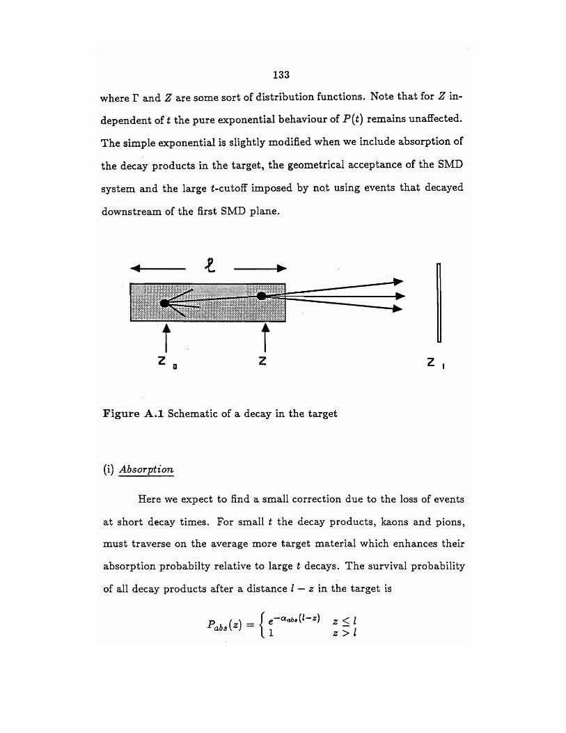
133
where r and Z are some sort of distribution functions. Note that for Zin-
dependent oft the pure exponential behaviour of P(t) remains unaffected.
The simple exponential is slightly modified when we include absorption of
the decay products in the target, the geometrical acceptance of the SMD
system and the large t-cutoff imposed by no.t using events that decayed
downstream of the first SMD plane.
t t Z D z z,
Figure A.1 Schematic of a decay in the target
(i) Absorption
Here we expect to find a small correction due to the loss of events
at short decay times. For small t the decay products, kaons and pions,
must traverse on the average more target material which enhances their
absorption probabilty relative to large t decays. The survival probability
of all decay products after a distance l - z in the target is
P ( ) - { e-aa0.(l-z) z :S l abs Z - l z > l
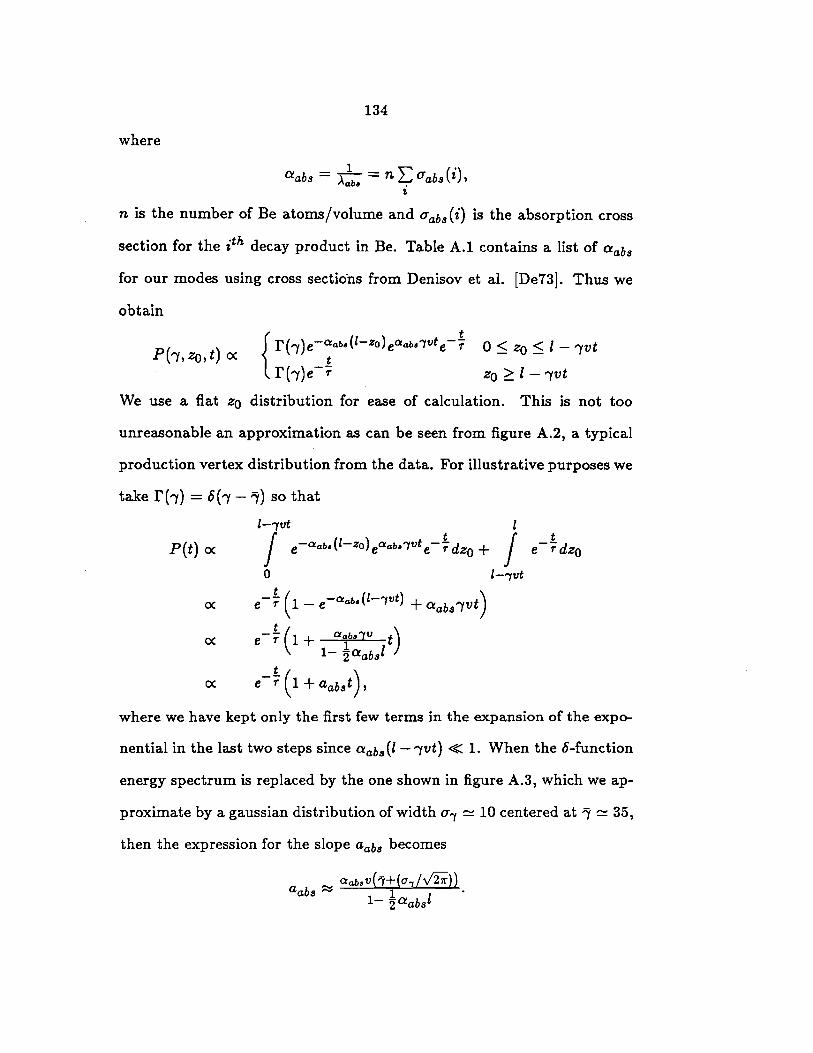
134
where
O!abs = x1- = n L <7abs(i), ab• .
i
n is the number of Be atoms /volume and a abs ( i) is the absorption cross
section for the ith decay product in Be. Table A.I contains a list of aabs
for our modes using cross sectio"ns from Denisov et al. [De73]. Thus we
obtain
{ r(l)e-ataba(l-zo)eaaba'1Vte-f Q::; ZQ::; l - /Vt
P(i,zo,t) ex r(l)e-r zo ~ l -1vt
We use a flat zo distribution for ease of calculation. This is not too
unreasonable an approximation as can be seen from figure A.2, a typical
production vertex distribution from the data. For illustrative purposes we
take r('"Y) = c5(1- '"Y) so that
l--yvt l
P(t) ex j e-°'ab•(l-zo) e°'ab•1"t e-* dzo + j 0 l-"'ftJt
ex e-* ( 1 - e-°'ab•(l-1vt) + °'abs'YVt)
ex e-* ( 1 + "'1••1" t) 1- 2aabsl
ex e-* ( 1 + aabst),
where we have kept only the first few terms in the expansion of the expo-
nential in the last two steps since aabs(l -1vt) < 1. When the a-function
energy spectrum is replaced by the one shown in figure A.3, which we ap-
proximate by a gaussian distribution of width a"'f ~ 10 centered at ry ~ 35,
then the expression for the slope aabs becomes
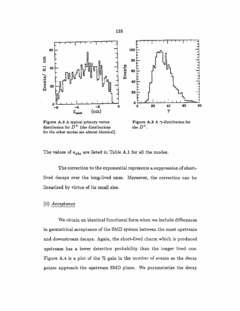
135
s (,)
...... c::i
' flJ .., s:: ~
> C:i:l
80
40
20
-2 {cm)
Figure A.2 A typical primary vertex distribution for v+ (the distributions for the other modes are almost identical).
0
Figure A.3 A /-distribution for the v+.
The values of aabs are listed in Table A.1 for all the modes.
The correction to the exponential represents a suppression of short-
lived decays over the long-lived ones. Moreover, the correction can be
linearized by virtue of its small size.
(ii) Acceptance
We obtain an identical functional form when we include differences
in geometrical acceptance of the SMD system between the most upstream
and downstream decays. Again, the short-lived charm which is produced
upstream has a lower detection probability than the longer lived one.
Figure A.4 is a plot of the % gain in the number of events as the decay
points approach the upstream SMD plane. We parameterize the decay
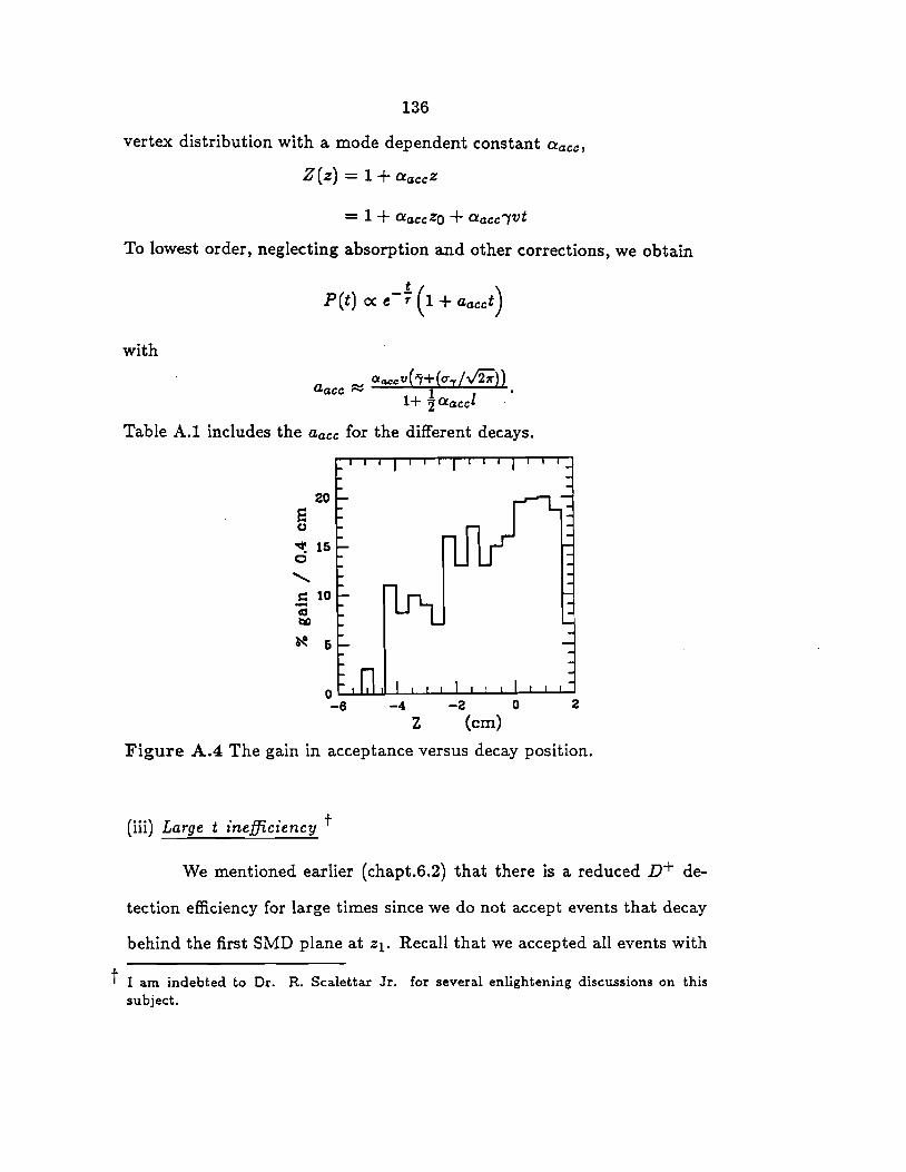
136
vertex distribution with a mode dependent constant aacc,
Z(z) = 1 + aaccZ
= 1 + aaccZQ + aacc/Vt
To lowest order, neglecting absorption and other corrections, we obtain
with
_ OacctJ( '1Y+(o-1/y"2;)} aacc - 1 .
1+ 2aaccl ·
Table A.1 includes the aacc for the different decays.
20
8 CJ
.qt 15 ci
' = 10 a; bO
l-e 5
-4 -2 0 z (cm)
2
Figure A.4 The gain in acceptance versus decay position.
(iii) Large t inefficiency t
We mentioned earlier ( chapt.6.2) that there is a reduced n+ de-
tection efficiency for large times since we do not accept events that decay
behind the first SMD plane at z1. Recall that we accepted all events with
t I a.m indebted to Dr. R. Sca.letta.r Jr. for several enlightening discussions on this subject.
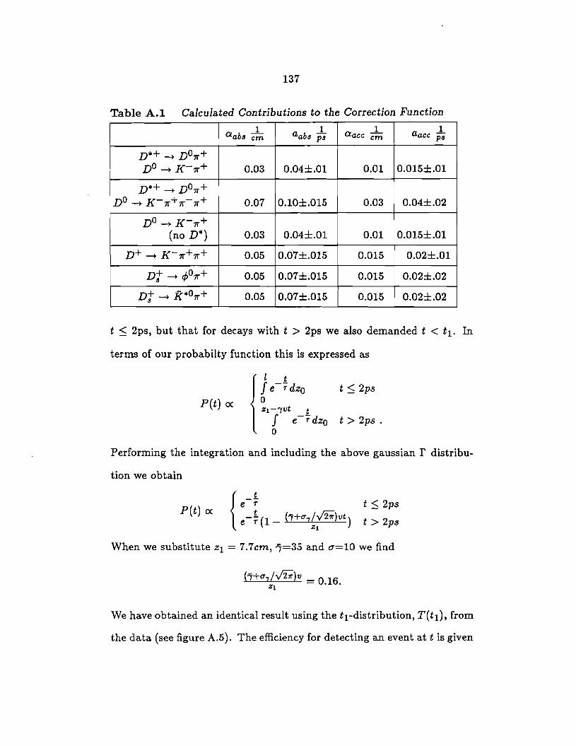
137
Table A.1 Calculated Contributions to the Correction Function
i a.abs cm
i aabs ps
i O.acc cm
i aacc ps
n•+-+ n°7r+ n°-+ K-7r+ 0.03 0.04±.01 0.01 0.015±.01
n•+-+ n°7r+ n°-+ K-7r+1r-7r+ 0.07 0.10±.015 0.03 0.04±.02
n°-+ K-7r+ (no D*) 0.03 0.04±.01 0.01 0.015±.01
n+ -+ K-7r+1r+ 0.05 0.07±.015 0.015 0.02±.01
nt -+ </>o'lr+ 0.05 0.07±.015 0.015 0.02±.02
n+-+ .f(*07r+ s 0.05 0.07±.015 0.015 0.02±.02
t ~ 2ps, but that for decays with t > 2ps we also demanded t < ti. In
terms of our probabilty function this is expressed as
P(t) ex t ~ 2ps
z1-1vt t J e - -:;: dzo t > 2 ps . 0
Performing the integration and including the above gaussian r distribu-
tion we obtain
P(t) ex
When we substitute zi = 7.7cm, '1=35 and a=lO we find
We have obtained an identical result using the ti-distribution, T(ti), from
the data (see figure A.5). The efficiency for detecting an event at t is given
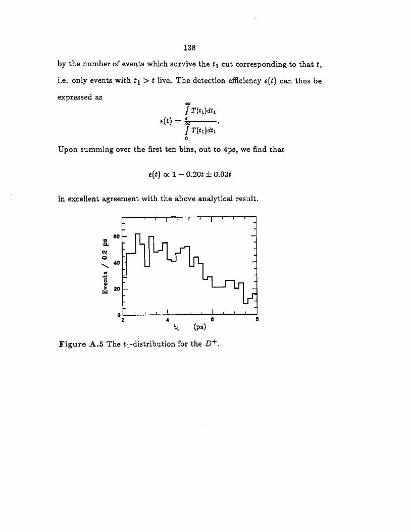
138
by the number of events which survive the ti cut corresponding to that t,
i.e. only events with ti > t live. The detection efficiency e(t) can thus be
expressed as 00
I T(ti)dt1 e(t) = ..;.._!c,-
J T(ti)dt1 0
Upon summing over the first ten bins, out to 4ps, we find that
e(t) oc 1 - 0.20t ± 0.03t
in excellent agreement with the above analytical result.
eo '1 a..
C\1 c:i
' 40
in ~
d w > 20
r:z:i
OL-..l.--L...-..L~L-..l--'---1..---'L--_.__._---1..___,
2 " 8 8
Figure A.5 The ti-distribution for then+.
139
REFERENCES
An83 B.Andersson,G.Gustafson,C.Ingelman,T.Sjostrand, Phys. Rep. 97, (1983), 31.
An87a J.C.Anjos et al., PRL 58, (1987), 311.
An87b J.C.Anjos et al., submitted to PRL, (1987). also see J.C.Anjos et al., Proceedings of the XXIII lnt'l Conference on High
Energy Physics, Berkeley CA, (1986).
Ap86 J.Appel,P.Ma.ntsch,M.Streetma.n,R.Robertson, Nucl. Instr. Meth. A243, (1986), 361.
Ba79 M.Bander,D.Silverman,A.Soni, Phys. Rev. Lett. 44, (1980), 7.
Ba85 M.Bauer,B.Stech, Phys. Lett. 152B, (1985), 380.
Ba86a D.Bartlett et al., Performance of the Cerenkov Counters in the Fermilab Tagged Photon Facility, preprint Colo-HEP-121, (1986).
Ba86b M.Bauer,B.Stech,M. Wirbel, Exclusive Non-Leptonic Decays of D- and Bmesons, preprint HD-THEP-86-19, Heidelberg, (1986).
Bh78 V.Bharadwaj et al.,Nucl. Instr. Meth. 155, (1978), 411.
Bh84 S.Bhadra, Inclusive Distributions of Diffractively Produced Neutral Kaons,
Lambdas and Anti-Lambdas, and Upper Limits on At' Production in High Energy IP interactions, Ph.D. thesis, University of Colorado at Boulder, (1984).
Bh85 V.Bharadwaj et al.,Nud. Instt. Meth. 228, (1985); 283.
Bi84 N.Bilic,B.Guberina,J.Trampetic, Nucl. Phys B248, (1984), 261.
Bi86 I.Bigi, On Our Theoretical Understanding of Charm Decays, SLAC-Pub-4067.
Bu86 A.Buras, Proceedings of the Int. Symp. on Production and Decay of Heavy Hadrons, Heidelberg, Germany, (1986), 179.
Ch83 L.Chau, Phys. Rep. 95, (1983), 1.
De73 S.Denisov et al., Nucl. Phys. B61, (1973), 62.
De83 B.Denby, Inelastic and Elastic Photoproduction of J / 1/; {3097), Ph.D. thesis, UC Santa Barbara., (1983).
Do86 J.F.Donoghue, Phys. Rev. D33, (1986), 1516.
Du82 A.Duncan, Characteristics of Hadronic States in High Energy Diffractive Photoproduction in Hydrogen, Ph.D. thesis, University of Colorado at Boulder, (1982).
Ea71
Es86
Fe86
Fo81
Fr79
Fr80
Ga75
Ge84
Go84
Gu79
Ha83
He81
Hi85
Jo78
Ka85
Kl84
Lii86
Me86
Na86
Or82
Ri86
140
W.Eadie,D.Drijard,F.James,M.Roos,B.Sadoulet, Statistical Methods in Experimental Physics, North-Holland/ American Elsevier, (1971).
P.Estabrooks, Aging Effects in a Large Driftchamber in the Fermilab Tagged Photon Spectrometer, preprint IPP /Ottawa-Carlton, 1986.
R.Fernow, Introduction to Experimental Particle Physics, Cambridge Univ. Press, (1986), p. 326.
M.Fontannaz,B.Pire,D.Schiff, Z. Phys. 011, (1981), 201.
A.G.Frodesen,O.Skjeggestad,H.Tf6fte, Probability and Statistics in Particle Physics, Universitetsforlaget, Oslo, 1979.
H.Fritzsch,P.Minkowski, Phys. Lett. 90B, (1980), 455.
M.K.Gaillard,B.W.Lee,J.L.Rosner, Rev. Mod. Phys. 41, (1975), 277.
H.Georgi, Weak Interactions and Modern Particle Theory, Benjamin-Cummings, 1984, p. 143.
T.Gottschalk, Hadronization and Fragmentation, Th 3810-CERN, (1984).
B.Guberina,S.Nussinov,R.Peccei,R.Riickl, Phys. Lett. 89B, (1979), 111.
G.Hartner et al., Nucl. Instr. Meth. 216, (1983), 113.
E.Heijne, Proceedings of a Workshop on Silicon Detectors for High Energy Physics, FNAL, 1981.
D.Hitlin, Proceedings of the Heavy Quark Workshop, FNAL, (1985), 10-1.
L.Jones,H.Wyld, Phys. Rev. D17, (1978), 759.
P.Karchin, IEEE NS-32, (1985), 612.
K.Kleinknecht, Detektoren fiir Teilchenstrahlung, Teubner, Stuttgart, (1984), p. 180.
V.Liith, Lifetimes of Heavy Flavour Particles, (1986), SLAC-Pub-4052.
S.Menary, A Study of TI-ansverse Momentum Distributions of Photoproduced Charged and Neutral D-mesons, Master's Thesis, University of Toronto, (1986).
T.Nash et al., Proceedings of the XXIII Int'I Conference on High Energy Physics, Berkeley CA, (1986).
J.Orear, Notes on Statistics for Physicists {revised}, (1982), preprint FNAL-48924.
G.de Rijk, Lifetime Measurements of Charmed Mesons with High Resolution Silicon Detectors, Ph.D. thesis, University of Amsterdam, 1986.
141
Rii.83 R.Rii.ckl, Weak Decays of Heavy Flavours, Habilitationsschrift, University of Munich, (1983).
Rii.86 R.Rii.ckl, Proceedings of the XXIII Int'I Conference on High Energy Physics, Berkeley CA, (1986).
Sh80 K.Shizuya, Phys. Lett. lOOB, (1981), 79.
So81 C.Sorenson, Phys. Rev. D23, (1981), 2618.
So86 M.Sokoloff et al., PRL 57, (1986), 3003.
Su84 D.Summers, A Study of the Decay DO ~ K- ?r+ ?ro in High Energy Pho-toproduction, Ph.D. thesis, UC Santa Barbara, (1984).
Su85 D.Summers, Nucl. Instr. Meth. 228, (1985), 290.
Ts74 Y.Tsai, Rev. Mod. Phys. 46, (1974), 815. Errata, Rev. Mod. Phys. 49, ( 1977), 421.