Transfer Function for a Simple Process - Inside Minesinside.mines.edu/~jjechura/ProcessDynamics/06_TransferFunctions.… · Transfer Function for a Simple Process ..... 1 Example

Colorado School of Mines CHEN403 Transfer Functions

John Jechura ([email protected]) - 1 - © Copyright 2017

April 23, 2017

Linear Open Loop Systems

Linear Open Loop Systems ................................................................................................................................... 1

Transfer Function for a Simple Process ......................................................................................................... 1

Example Transfer Function — Mercury Thermometer ........................................................................... 2

Desirability of Deviation Variables .............................................................................................................. 3

Transfer Function for Process with Multiple Inputs and/or Multiple Outputs............................. 3

Example Transfer Function — Stirred Tank Heater ................................................................................. 5

Transfer Function of Process in Series ........................................................................................................... 9

Poles & Zeros of a Transfer Function............................................................................................................... 9

Example — Poles & Zeros of a Transfer Function .............................................................................. 12

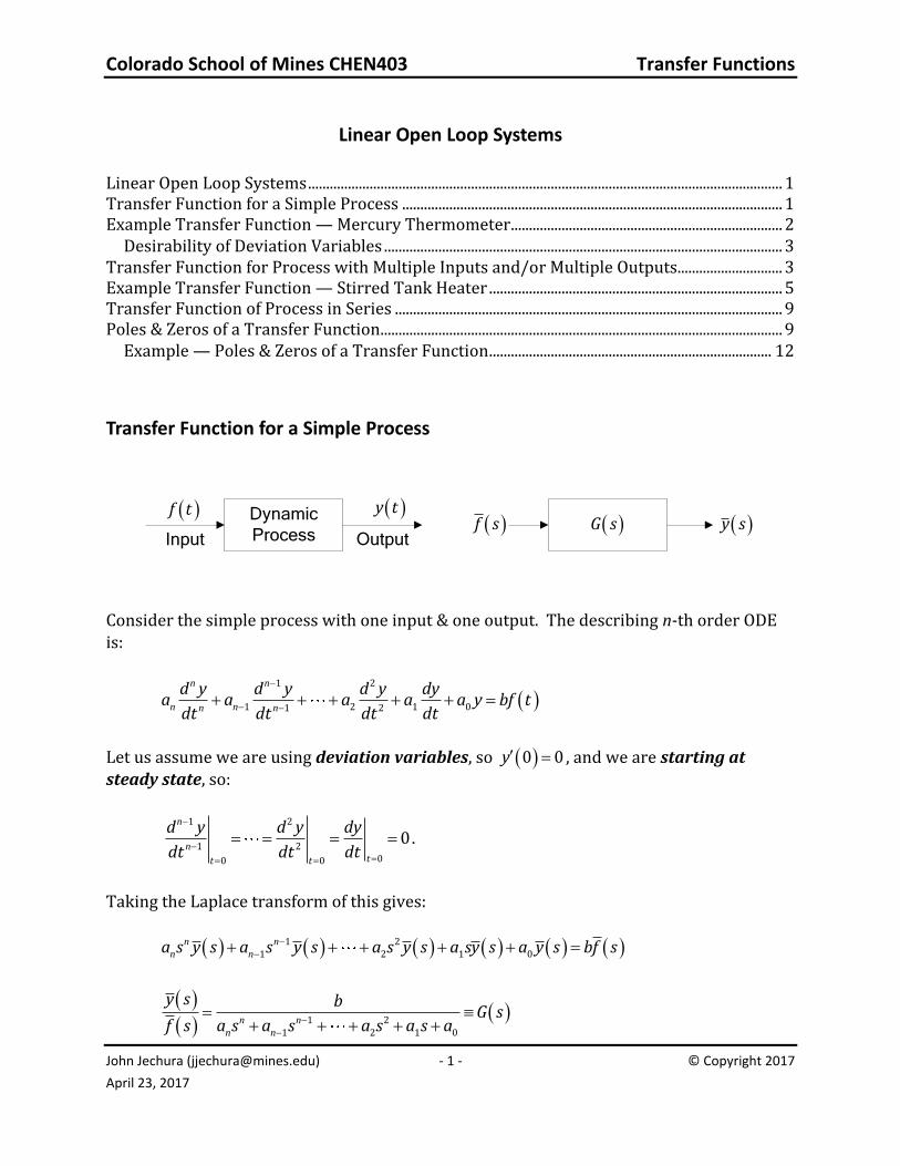
Transfer Function for a Simple Process

Dynamic

Process

f t y t

Input Output

f s y s G s

Consider the simple process with one input & one output. The describing n-th order ODE is:

1 2

1 2 1 01 2

n n

n nn n

d y d y d y dya a a a a y bf tdt dt dt dt

Let us assume we are using deviation variables, so 0 0y , and we are starting at steady state, so:

1 2

1 200 0

0n

ntt t

d y d y dy

dt dt dt.

Taking the Laplace transform of this gives:

1 2

1 2 1 0n n

n na s y s a s y s a s y s a sy s a y s bf s

1 2

1 2 1 0n n

n n

y s bG s

f s a s a s a s a s a



April 23, 2017

where G s is defined as the transfer function and the simple diagram is called the block diagram for the process.

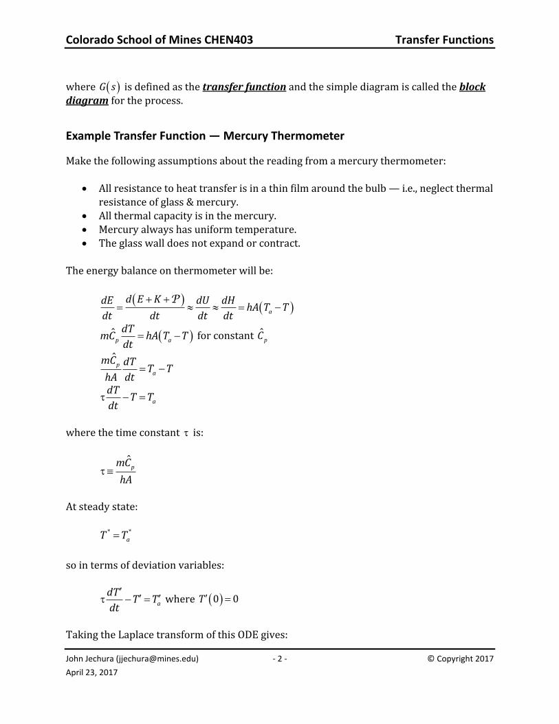
Example Transfer Function — Mercury Thermometer

Make the following assumptions about the reading from a mercury thermometer:

• All resistance to heat transfer is in a thin film around the bulb — i.e., neglect thermal resistance of glass & mercury.

• All thermal capacity is in the mercury. • Mercury always has uniform temperature. • The glass wall does not expand or contract.

The energy balance on thermometer will be:

P

a

d E KdE dU dHhA T T

dt dt dt dt

ˆp a

dTmC hA T T

dt for constant ˆ

pC

ˆp

a

mC dTT T

hA dt

a

dTT T

dt

where the time constant is:

ˆpmC

hA

At steady state:

* *aT T

so in terms of deviation variables:

a

dTT T

dt where 0 0T

Taking the Laplace transform of this ODE gives:



April 23, 2017

1 as T T

so the transfer function is:

1

1a

TG s

T s

So, we would expect the heat transfer resistance around a thermometer to be a 1st order system. Desirability of Deviation Variables

If we didn’t use deviation variables the Laplace transform of the ODE would be:

0a a

dTT T sT T T T

dt

1 0as T T T

*

10

1 1

1

1 1

a

a a

T T Ts s

T Ts s

Now there are two inputs & two transfer functions: one for the driving function ( aT t or

aT s ) and one for the initial condition ( *aT ).

Transfer Function for Process with Multiple Inputs and/or Multiple Outputs

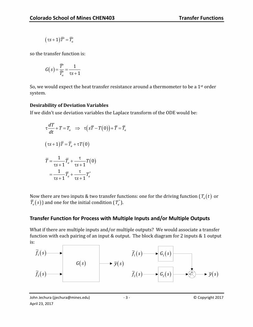
What if there are multiple inputs and/or multiple outputs? We would associate a transfer function with each pairing of an input & output. The block diagram for 2 inputs & 1 output is:

1f s

2f s

y s G s

++

1f s

2G s

1G s

2f s y s



April 23, 2017

The overall relationship for y s would be:

1 1 2 2y s G s f s G s f s

For n inputs and one output, then:

1 1 2 2 3 3 n ny s G s f s G s f s G s f s G s f s

1

n

i ii

y s G s f s

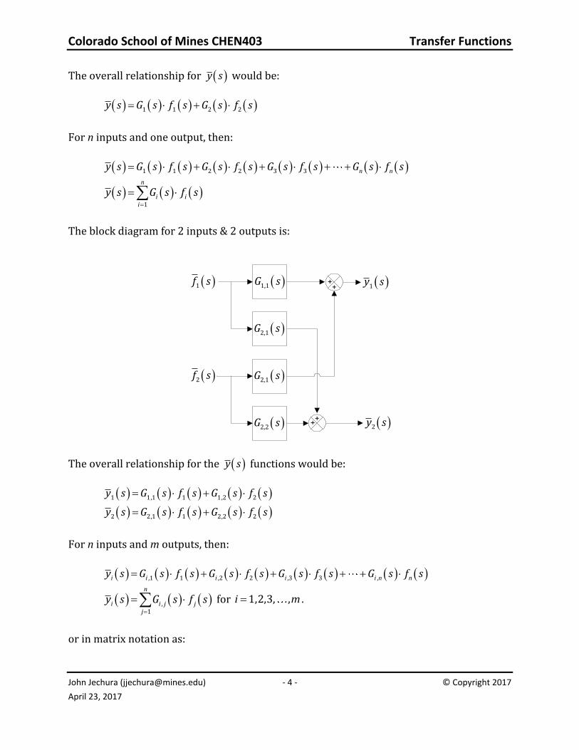
The block diagram for 2 inputs & 2 outputs is:

++

1f s

2,2G s

2,1G s 2f s

2y s

2,1G s

1,1G s ++

1y s

The overall relationship for the y s functions would be:

1 1,1 1 1,2 2y s G s f s G s f s

2 2,1 1 2,2 2y s G s f s G s f s

For n inputs and m outputs, then:

,1 1 ,2 2 ,3 3 ,i i i i i n ny s G s f s G s f s G s f s G s f s

,1

n

i i j jj

y s G s f s for 1,2,3, ,i m .

or in matrix notation as:



April 23, 2017

s s sy G f

where sy is a column vector of length m , sf is a column vector of length n , and sG is a m n rectangular matrix. sG is called the transfer function matrix.

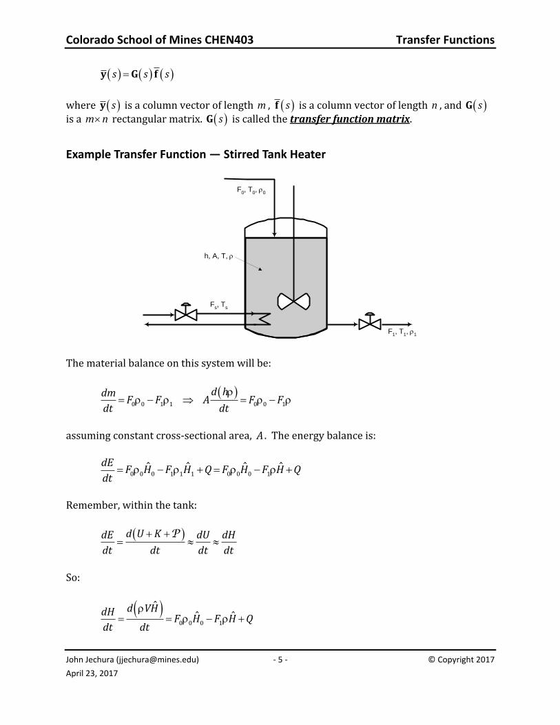
Example Transfer Function — Stirred Tank Heater

F0, T

0,

0

F1, T

1,

1

h, A, T,

Fs, T

s

The material balance on this system will be:

0 0 1 1 0 0 1

d hdmF F A F F

dt dt

assuming constant cross-sectional area, A . The energy balance is:

0 0 0 1 1 1 0 0 0 1ˆ ˆ ˆ ˆdE

F H F H Q F H F H Qdt

Remember, within the tank:

Pd U KdE dU dH

dt dt dt dt

So:

0 0 0 1

ˆˆ ˆ

d VHdHF H F H Q

dt dt



April 23, 2017

If we assume that the enthalpy can be expressed as:

ˆˆ ˆp ref refH C T T H

then with ˆ 0refH & 0refT :

0 0 0 1ˆ ˆ ˆp p p

dVC T F C T F C T Q

dt

0 0 0 1ˆ ˆ ˆp p p

dC VT F C T F C T Qdt

0 0 0 1 ˆp

d QVT F T F T

dt C

If we assume constant , then:

0 1

dhA F Fdt

and:

0 0 1 ˆp

d QA hT F T F Tdt C

0 10 ˆ

p

F Fd QhT T T

dt A A AC

0 0 1 ˆp

dh dT QTA hA F T F Tdt dt C

Inserting the material balance:

0 1 0 0 1 ˆp

dT QT F F hA F T F T

dt C

0 0 ˆp

dT QhA F T T

dt C where h h t .

If we make the assumption that / 0dh dt then constantV hA & 0 1F F , so:

0 0 ˆp

dT QV F T Tdt C



April 23, 2017

If we are using steam for the heating medium, then we could relate the rate of heat added, Q , to the steam temperature, sT , as:

sQ UA T T .

So:

0 0 ˆs

p

UA T TdTV F T Tdt C

0 0 0 ˆ s

p p

dT UA UAV F T F T Tdt C C

0 00ˆ ˆ s

p p

F FdT UA UAT T T

dt V VVC VC

0

1 1s

F F

dTK T T KT

dt

0

1s

F

dTaT T KT

dt

where:

01

F

F

V,

ˆp

UAK

VC, and

1

F

a K .

At steady state:

* * *0

1s

F

aT T KT

so:

0

1s

F

dTaT T KT

dt

where the deviation variables are defined as:

*T T T , *0 0 0T T T , and *

s s sT T T .



April 23, 2017

Note that this equation shows how the stirred tank fluid temperature is affected by changes in the other temperatures.

In this Chapter we will convert this equation into one involving transfer functions. Taking the Laplace transform of the equation gives:

0

10 s

F

sT T aT T KT

0

1s

F

sT aT T KT

0

1s

F

s a T T KT

0

1 Fs

KT T T

s a s a

This shows that we have two transfer functions:

0 0 s sT G s T G s T

where:

0

1/ FG ss a

and

s

KG s

s a

A block diagram for the stirred tank heater can be drawn as follows.

+

+

0T s

K

s a

1/ F

s a

sT s

T s



April 23, 2017

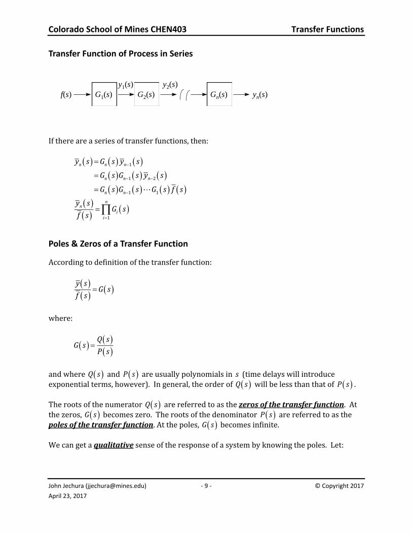
Transfer Function of Process in Series

f(s) G1(s) G2(s) Gn(s) yn(s)

y2(s)y1(s)

If there are a series of transfer functions, then:

1

1 2

1 1

n n n

n n n

n n

y s G s y s

G s G s y s

G s G s G s f s

1

nn

ii

y sG s

f s

Poles & Zeros of a Transfer Function

According to definition of the transfer function:

y s

G sf s

where:

Q s

G sP s

and where Q s and P s are usually polynomials in s (time delays will introduce exponential terms, however). In general, the order of Q s will be less than that of P s . The roots of the numerator Q s are referred to as the zeros of the transfer function. At the zeros, G s becomes zero. The roots of the denominator P s are referred to as the poles of the transfer function. At the poles, G s becomes infinite. We can get a qualitative sense of the response of a system by knowing the poles. Let:



April 23, 2017

r s

f sq s

Since:

Q

GP

ss

s

then:

Q s r s

y s G s f sP s q s

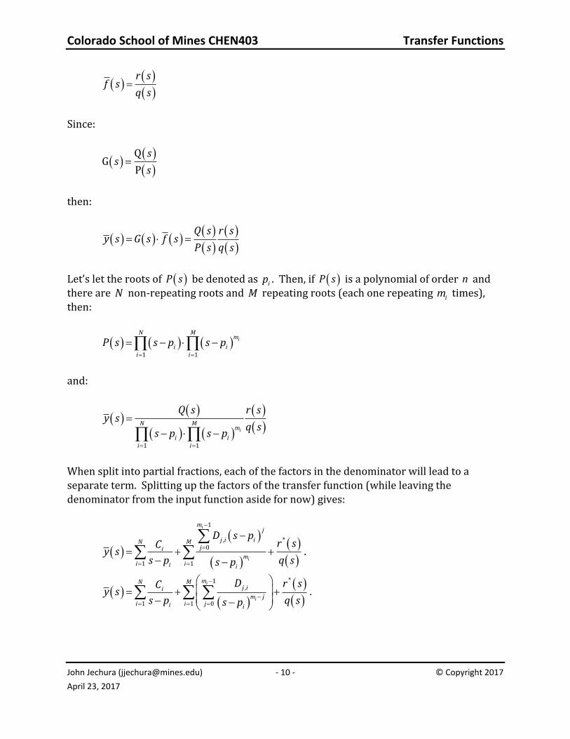
Let’s let the roots of P s be denoted as ip . Then, if P s is a polynomial of order n and there are N non-repeating roots and M repeating roots (each one repeating im times), then:

1 1

i

N Mm

i ii i

P s s p s p

and:

1 1

i

N Mm

i ii i

Q s r sy s

q ss p s p

When split into partial fractions, each of the factors in the denominator will lead to a

separate term. Splitting up the factors of the transfer function (while leaving the denominator from the input function aside for now) gives:

1

*,0

1 1

i

i

mj

j i iN Mji

mi ii i

D s pr sC

y ss p q ss p

.

*1

,

1 1 0

i

i

mN Mj iim j

i i ji i

D r sCy s

s p q ss p.



April 23, 2017

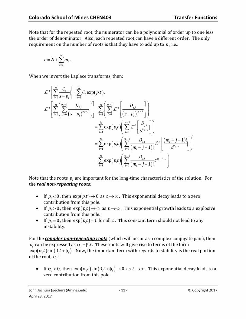
Note that for the repeated root, the numerator can be a polynomial of order up to one less the order of denominator. Also, each repeated root can have a different order. The only requirement on the number of roots is that they have to add up to n , i.e.:

1

M

ii

n N m .

When we invert the Laplace transforms, then:

L 1

1 1

expN N

ii i

i ii

CC p t

s p.

L L

L

L

1 1, ,1 1

1 0 1 0

1,1

1 0

1, 1

1 0

exp

1 !exp

1 !

exp

i i

i i

i

i

i

i

m mM Mj i j i

m j m ji j i ji i

mMj i

i m ji j

mMj i i

i m ji j i

D D

s p s p

Dp t

s

D m jp t

m j s

p

1

, 1

1 0 1 !

i

i

mMj i m j

ii j i

Dt t

m j

.

Note that the roots ip are important for the long-time characteristics of the solution. For the real non-repeating roots:

• If 0ip , then exp 0ip t as t . This exponential decay leads to a zero contribution from this pole.

• If 0ip , then exp ip t as t . This exponential growth leads to a explosive contribution from this pole.

• If 0ip , then exp 1ip t for all t . This constant term should not lead to any instability.

For the complex non-repeating roots (which will occur as a complex conjugate pair), then

ip can be expressed as i ii . These roots will give rise to terms of the form

exp sini i it t . Now, the important term with regards to stability is the real portion of the root, i :

• If 0i , then exp sin 0i i it t as t . This exponential decay leads to a zero contribution from this pole.



April 23, 2017

• If 0i , then exp sini i it t as t . This exponential growth leads to a explosive contribution from this pole.

• If 0i , then exp sin sini i i i it t t for all t . This term will lead to a stable oscillation.

For the repeating roots, the situation is similar. The polynomial term will always grow towards infinity as t , so the behavior of the exponential term will dictate the overall behavior.

• If 0ip or 0i , then the exponential term will go to zero as t and the entire term will also go to zero. This exponential decay leads to a zero contribution from this pole.

• If 0ip or 0i , then the exponential term will grow to infinity as t and the entire term will also grow to infinity. This exponential growth leads to an explosive contribution from this pole.

• If 0ip or 0i , then the polynomial term will dictate the behavior for t . This polynomial term will lead to an explosive contribution from this pole..

So, in general:

• If 0i , stable contribution from this pole. • If 0i , unstable contribution from this pole. • If 0i , stable contribution only if non-repeated root — unstable contribution if

repeated root. Example — Poles & Zeros of a Transfer Function

Given the transfer function:

4 3 23 5 4 2

Q s Q sG s

P s s s s s

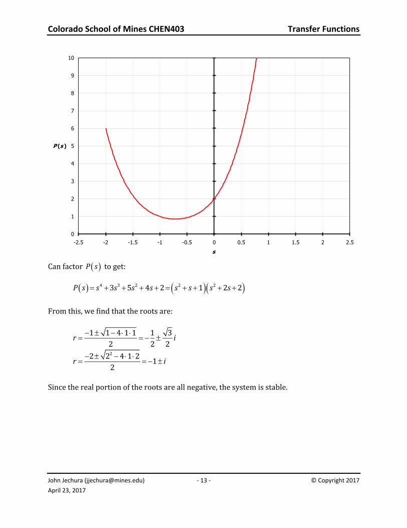
find the zeros & determine if stable. The following chart shows the characteristics of P s vs. s . Note that there are no real roots.



April 23, 2017

0

1

2

3

4

5

6

7

8

9

10

-2.5 -2 -1.5 -1 -0.5 0 0.5 1 1.5 2 2.5

s

P (s )

Can factor P s to get:

4 3 2 2 23 5 4 2 1 2 2P s s s s s s s s s

From this, we find that the roots are:

1 1 4 1 1 1 3

2 2 2r i

22 2 4 1 2

12

r i

Since the real portion of the roots are all negative, the system is stable.

Documents

Transfer Function for a Simple Process - Inside Minesinside.mines.edu/~jjechura/ProcessDynamics/06_TransferFunctions.… · Transfer Function for a Simple Process ..... 1 Example