Colorado School of Mines CHEN403 Mathematical Models ...inside.mines.edu/~jjechura/ProcessDynamics/02_HeatMaterialBalance... · Setting up the Mathematical Model Review of Heat &

Colorado School of Mines CHEN403 Mathematical Models

John Jechura ([email protected]) - 1 - © Copyright 2017 April 23, 2017

Setting up the Mathematical Model Review of Heat & Material Balances

Topic Summary ......................................................................................................................................................... 1

Introduction ................................................................................................................................................................ 2

Conservation Equations ........................................................................................................................................ 3

Use of Intrinsic Variables ................................................................................................................................. 4

Well-Mixed Systems ........................................................................................................................................... 4

Conservation of Total Mass: ............................................................................................................................ 4

Component Balances .......................................................................................................................................... 5

Energy balance: .................................................................................................................................................... 5

Additional Relationships ....................................................................................................................................... 6

Exceptions to Well-Mixed Process Assumptions ........................................................................................ 8

Processes with Dead Time ............................................................................................................................... 8

Flow Approximated by Combination of Well-Mixed Blocks ............................................................. 8

Examples ...................................................................................................................................................................... 9

Tank Liquid Level with Flow Through Valve........................................................................................... 9

State Variables: ..................................................................................................................................................... 9

Total Mass Balance Leads to a Volume Balance: .................................................................................... 9

Other Tank Geometries ............................................................................................................................. 10

Right Circular Cone ..................................................................................................................................... 10

Horizontal Cylinder .................................................................................................................................... 10

Tank flow — Change in Inlet Concentration ........................................................................................ 11

Overall & Component Mass Balances: ................................................................................................ 11

Component Material Balance: ................................................................................................................ 12

Using Concentration ................................................................................................................................... 12

Using Mass Fraction ................................................................................................................................... 12

Tank Flow — Chemical Reaction ............................................................................................................... 13

Tank Flow — Change in Input Stream’s Temperature ..................................................................... 14

State Variables: ............................................................................................................................................. 15

Initial state:..................................................................................................................................................... 15

Transient solutions ..................................................................................................................................... 15

What if the heat input is described by Newton’s law?................................................................. 16

Example – Tank Flow Controlled by Valve ............................................................................................ 17

Bernoulli’s Law: ............................................................................................................................................ 17

Total mass balance reduces to volume balance for constant density: ................................. 18

Example: Chemical Reaction........................................................................................................................ 19

Topic Summary

• Definition of well-mixed system. Combining well-mixed sub-processes to describe

overall process that is not well-mixed.



• Dynamic equations from material & energy balance equations • Typical simplifications & modifications • Additional relationships

We will show that certain dynamic relations typically come most directly from certain conservation equations. These typical relationships are shown in the following table.

Conservation Equation Typical Dynamic Relation

Overall Material Balance Outlet volumetric flowrates vs. inlet rates Liquid: Liquid level in system vs. time Gas: Gas pressure in system vs. time

Component Balance Outlet concentration vs. time Outlet mole/mass fraction vs. time

Thermal Energy Balance Outlet temperature vs. time

Introduction

Transient behavior of a process: • Start up. • “Steady state” — random disturbances. • Change of set points. • Shut down.

Steps for math modeling:

• Develop the relationships/equations. • Simplify. • Solve:

Analytical — Laplace transforms

Numerial — Euler, Runge-Kutte methods Needs of math model:

• Quantities whose values describe the nature of the process. These are the state variables.

• Equations that use the quantities & describe how the variables change with time.

For algebraic equations, where N is the number of variables & E is the number of independent equations:

• E N , deterministic system. • E N , under-determined system. • E N , over-determined system.



For differential conditions, also need boundary conditions. For transient problems, these are normally initial conditions. We will mostly be working with lumped systems – i.e., there will be no spatial variation. Often termed as a well-mixed system.

Conservation Equations

We will use the basic principles of chemical engineering to guide us in our descriptions of our dynamic processes: conservation of mass, energy, & momentum. So, the types of conservation equations will be:

• The overall mass balance. • Component/chemical species balance (including reaction rate terms). • Thermal energy/heat balance. • Momentum balance (though we won’t usually work with this in this class).

General form of the “stuff” balance equation:

Rate of Rate Rate Rate of Rate of

Accumulation In Out Generation Consumption

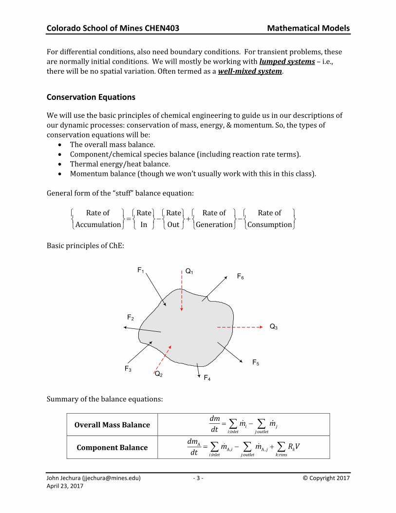
Basic principles of ChE:

F1

F3

F4

F5

F6

Q1

Q2

Q3

F2

Summary of the balance equations:

Overall Mass Balance : :

i ji inlet j outlet

dmm m

dt

Component Balance AA, A,

: : :i j k

i inlet j outlet k rxns

dmm m R V

dt



AA, A,

: : :i j k


dNN N r V

dt

Energy Balance ,: :

i j k s mi inlet j outlet k m

dEE E Q W

dt

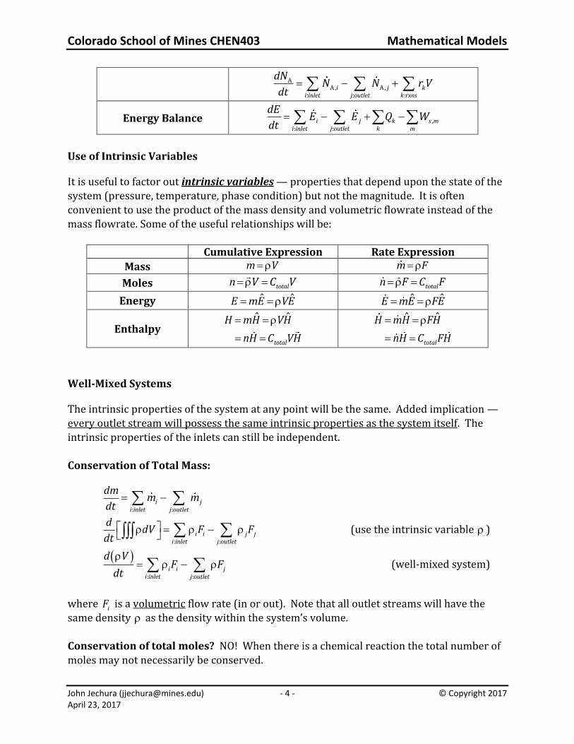
Use of Intrinsic Variables

It is useful to factor out intrinsic variables — properties that depend upon the state of the system (pressure, temperature, phase condition) but not the magnitude. It is often convenient to use the product of the mass density and volumetric flowrate instead of the mass flowrate. Some of the useful relationships will be:

Cumulative Expression Rate Expression

Mass m V m F

Moles totaln V C V totaln F C F

Energy ˆ Ê mE VE ˆ Ê mE FE

Enthalpy

ˆ ˆ

total

H mH VH

nH C VH

ˆ ˆ

total

H mH FH

nH C FH

Well-Mixed Systems

The intrinsic properties of the system at any point will be the same. Added implication — every outlet stream will possess the same intrinsic properties as the system itself. The intrinsic properties of the inlets can still be independent. Conservation of Total Mass:

: :

i ji inlet j outlet

dmm m

dt

: :i i j j

i inlet j outlet

ddV F F

dt (use the intrinsic variable )

: :

i i ji inlet j outlet

d VF F

dt (well-mixed system)

where iF is a volumetric flow rate (in or out). Note that all outlet streams will have the same density as the density within the system’s volume. Conservation of total moles? NO! When there is a chemical reaction the total number of

moles may not necessarily be conserved.



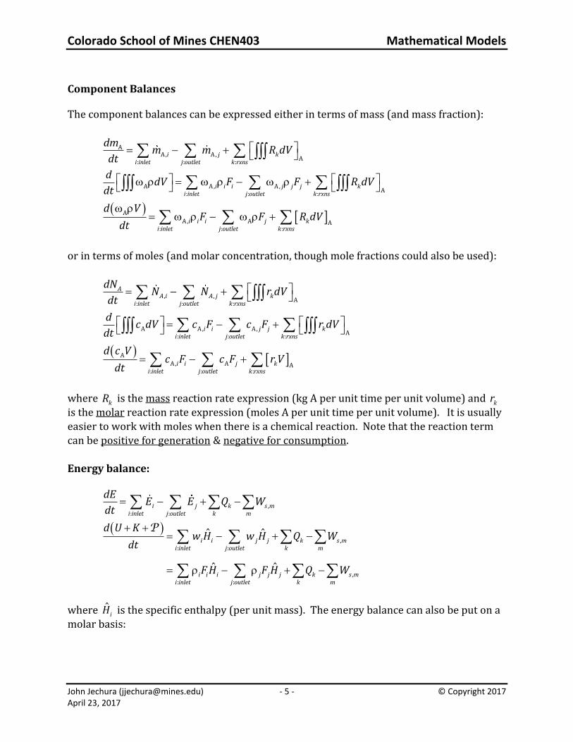
Component Balances

The component balances can be expressed either in terms of mass (and mass fraction):

AA, A,

A: : :

i j ki inlet j outlet k rxns

dmm m R dV

dt

A A , A ,

A: : :

i i i j j j ki inlet j outlet k rxns

ddV F F R dV

dt

A

A , A A: : :

i i i j ki inlet j outlet k rxns

d VF F R dV

dt

or in terms of moles (and molar concentration, though mole fractions could also be used):

, ,

A: : :

AA i A j k


dNN N r dV

dt

A A, A,

A: : :

i i j j ki inlet j outlet k rxns

dc dV c F c F r dV

dt

A

A , A A: : :

i i j ki inlet j outlet k rxns

d c Vc F c F r V

dt

where kR is the mass reaction rate expression (kg A per unit time per unit volume) and kr is the molar reaction rate expression (moles A per unit time per unit volume). It is usually easier to work with moles when there is a chemical reaction. Note that the reaction term can be positive for generation & negative for consumption. Energy balance:

,: :

i j k s mi inlet j outlet k m

dEE E Q W

dt

P,

: :

,: :

ˆ ˆ

ˆ ˆ

i i j j k s mi inlet j outlet k m

i i i j j j k s mi inlet j outlet k m

d U Kw H w H Q W

dt

F H F H Q W

where ˆ

iH is the specific enthalpy (per unit mass). The energy balance can also be put on a molar basis:



P

,: :

i i j j k s mi inlet j outlet k m

d U KN H N H Q W

dt

where iH is the specific enthalpy per unit mole basis.

There are additional assumptions normally made to the energy balance:

P

,: :

ˆ î i i j j j k s m

i inlet j outlet k m

d U KF H F H Q W

dt

,: :



dUF H F H Q W

dt (internal energy dominant term)

For liquid systems we will generally use the assumption that U H :

,: :



dHF H F H Q W

dt

,

: :

ˆ ˆ î i i j j j k s m


dHdV F H F H Q W

dt

,: :

ˆˆ ˆ

i i i j k s mi inlet j outlet k m

d HVF H F H Q W

dt (well-mixed).

For gas systems this is not necessarily the case. However, since we ultimately want a dynamic expression for temperature this is not a significant problem.

,: :

ˆ ˆ î i i j j j k s m


dUdV F H F H Q W

dt

,: :

ˆˆ ˆ

i i i j k s mi inlet j outlet k m

d UVF H F H Q W

dt

(well-mixed).

Additional Relationships

These are the basic equations, but now we also need relationships to the measured process variables. Relationship between mass & volume: m V Ah (for constant cross sectional area)

m F



Thermodynamic relationships:

ˆ ˆˆ ˆ

ref

ref

T

p ref p p ref

TP

T

ref p p ref

T

HC H H C dT C T T

T

H H C dT C T T

U H PV H (for liquid systems) U H RT (for ideal gas systems) Equations of state relating density to pressure, temperature, & composition:

, ,T P x (the equation of state). Some simple equations of state:

i ii

PM Px M

RT RT (ideal gas)

1 1i i i

i ii i

x M

M (ideal volume of mixing/additive volumes)

Energy relationships:

2 21 1

2 2K mv Vv

P 0 0mg h h Vg h h (gravitational potential energy. May be other forms)

Relationship between heat transfer rate & temperature driving force:

aQ UA T T (Newton’s law of heating/cooling)

4 41 1 1 12 2Q A T T (Kirschoff’s law of radiant heat exchange)

Relationship between flow through a valve & pressure driving force:

p vF p F A p C h (non-linear valve flow expression)

Chemical reaction rate relationships:

, ,A Ar r T Px (the reaction rate function). For example:

/0

E RTA A Ar k T c k e c (1st order reaction)

2 / 20

E RTA A Ar k T c k e c or /

0E RT

A A Br k e c c (2nd order reactions)

where /0

E RTk T k e is the Arrenhius rate expression.



Exceptions to Well-Mixed Process Assumptions

Processes with Dead Time

One exception to the well-mixed assumption is when there is some piece to the process that introduces a significant time delay between when something happens and when this might be measured. One can picture the situation as being similar to plug flow through a pipe — the material does not change in the pipe, but there is a time difference between when it enters and when it reappears at the other end. For example, if we are interested in the temperature at the exit of a tank, oT , but the thermocouple is in a pipe a distance L away, then there will be a delay before the temperature can be measured. This time delay,

ot , can be estimated from:

0 0

distance

velocity /c

o

c

LALt

F A F

where: cA is the cross sectional area of the pipe. oF is the volumetric flow rate. If there is no heat loss in the pipe then the relationships between the outlet temperature of the tank at that temperature measured, mT , is:

m o oT t T t t .

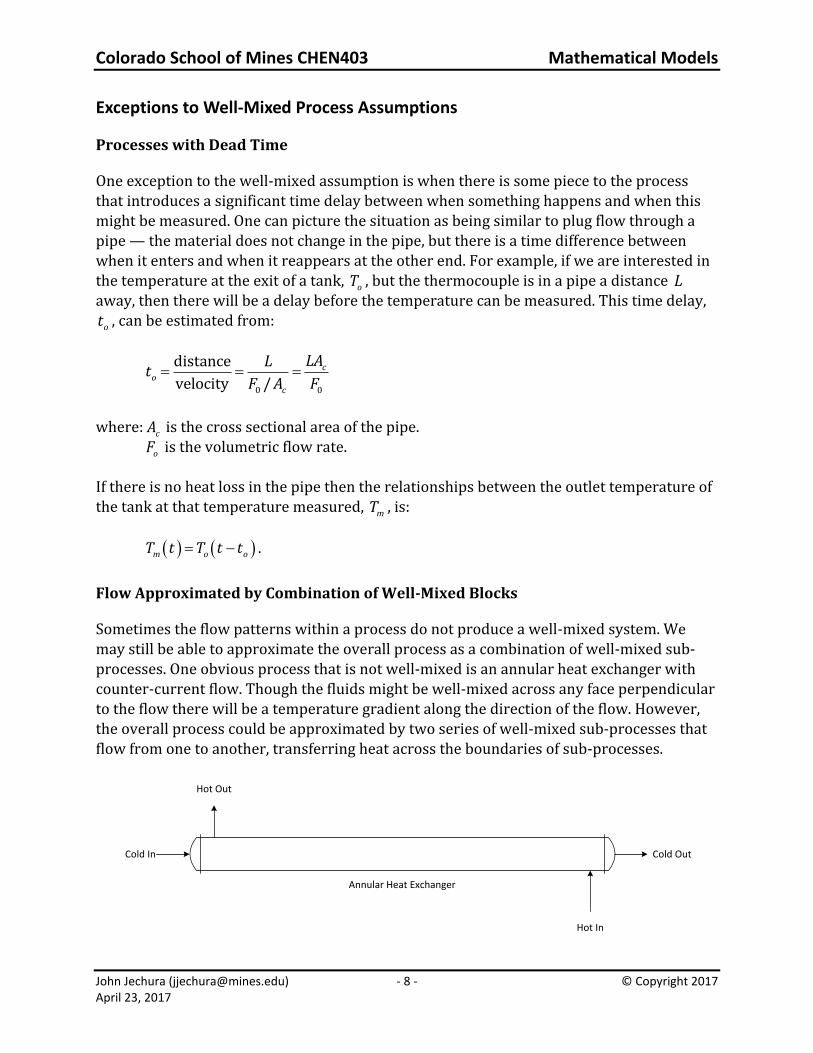
Flow Approximated by Combination of Well-Mixed Blocks

Sometimes the flow patterns within a process do not produce a well-mixed system. We may still be able to approximate the overall process as a combination of well-mixed sub-processes. One obvious process that is not well-mixed is an annular heat exchanger with counter-current flow. Though the fluids might be well-mixed across any face perpendicular to the flow there will be a temperature gradient along the direction of the flow. However, the overall process could be approximated by two series of well-mixed sub-processes that flow from one to another, transferring heat across the boundaries of sub-processes.

Annular Heat Exchanger

Cold OutCold In

Hot Out

Hot In



Cold In

Hot Out

Cold Out

Hot In

Examples

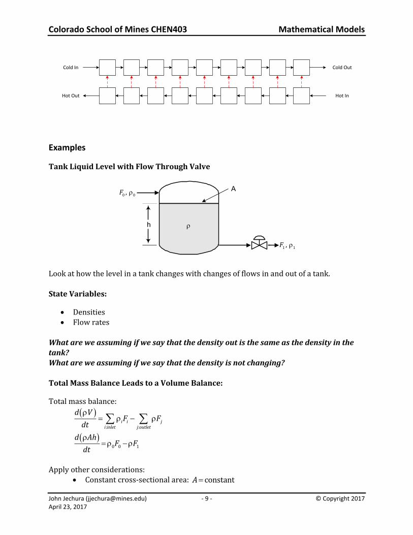
Tank Liquid Level with Flow Through Valve

h

A0 0, F

1 1, F

Look at how the level in a tank changes with changes of flows in and out of a tank.

State Variables:

• Densities • Flow rates

What are we assuming if we say that the density out is the same as the density in the tank? What are we assuming if we say that the density is not changing? Total Mass Balance Leads to a Volume Balance:

Total mass balance:

: :


d VF F

dt

0 0 1

d AhF F

dt

Apply other considerations: • Constant cross-sectional area: constantA



• Constant density: 1 0 Total mass balance becomes a volume balance leading to a differential equation for the level in the tank with respect to time:

0 1

dhA F F

dt

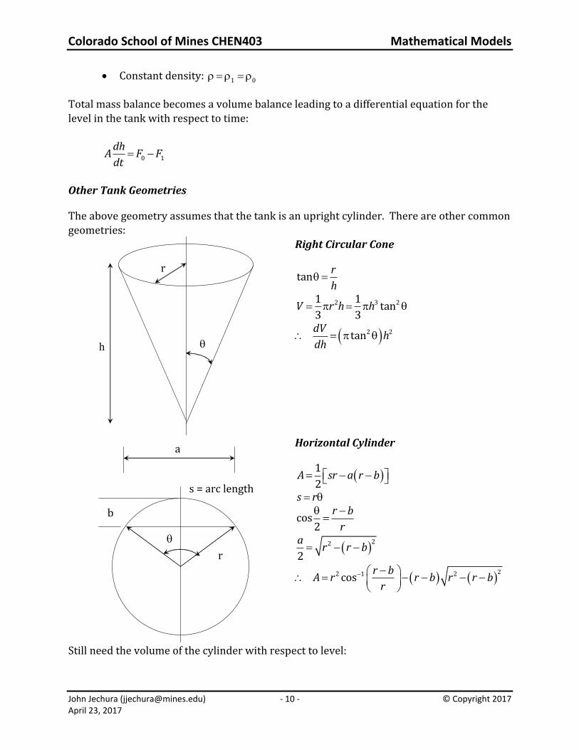
Other Tank Geometries

The above geometry assumes that the tank is an upright cylinder. There are other common geometries:

h

r

Right Circular Cone

tanr

h

2 3 21 1tan

3 3V r h h

2 2tandV

hdh

b

r

s = arc length

a

Horizontal Cylinder

1

2A sr a r b

s r cos

2

r b

r

22

2

ar r b

22 1 2cosr b

A r r b r r br

Still need the volume of the cylinder with respect to level:



22 1 2

22 2 1 2

cos

cos

r hLr L r h r r h if h r

rV

h rr L Lr L h r r h r if h r

r

The amazing part is that the derivative is the same for both halves:

2 2dV

L h r hdh

Sphere. Using similar definitions are for the horizontal cylinder:

2

23

13

3

2 12

3 3

h r h if h r

V

r r h r h if h r

and, again, the derivative is the same for both halves:

2dV

h r hdh

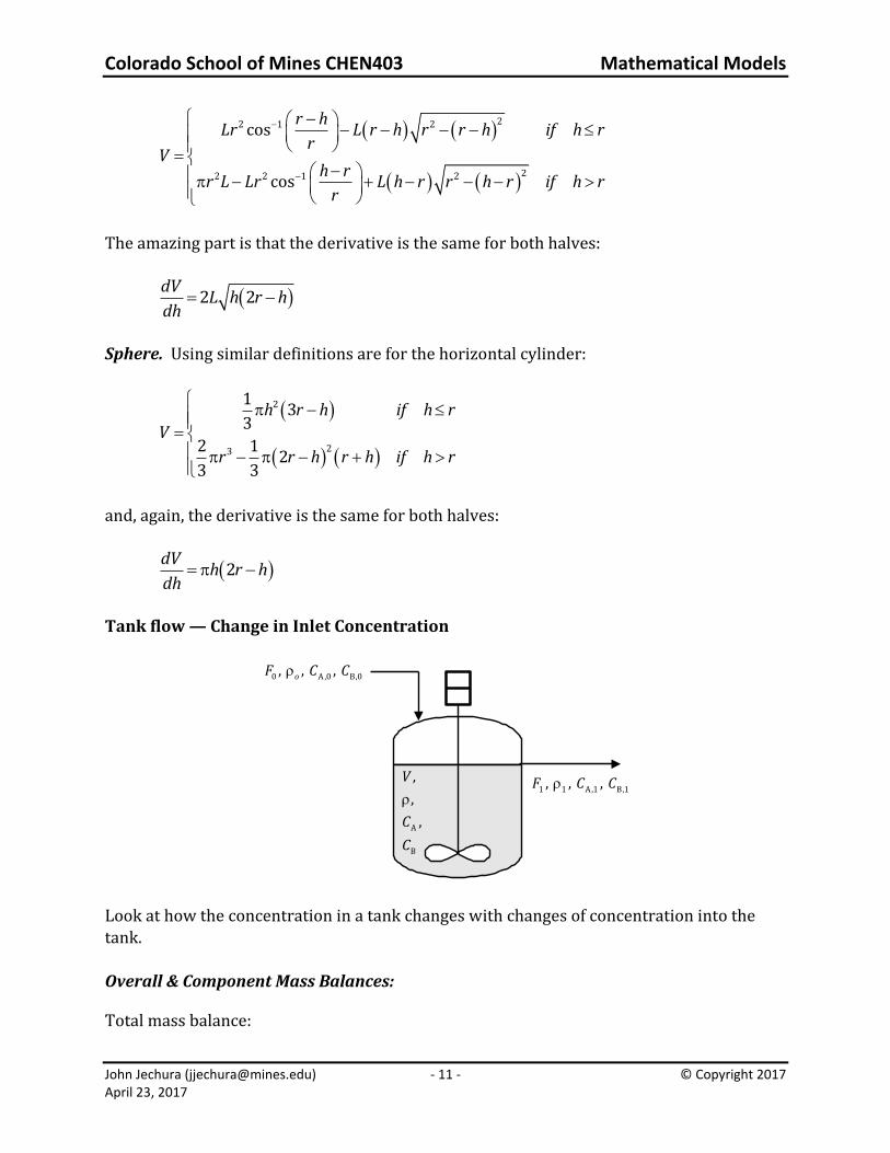
Tank flow — Change in Inlet Concentration

0 A ,0 B,0, , , oF C C

1 1 A ,1 B,1, , , F C C

A

B

,

,

,

V

C

C

Look at how the concentration in a tank changes with changes of concentration into the tank. Overall & Component Mass Balances:

Total mass balance:



: :


d VF F

dt

0 0 1

dV F F

dt

What have we assumed here? Constant volume overflow (& well-mixed). If we assume constant density: 0 1 1 00 F F F F .

Component Material Balance:

We can deal with multi-component mixtures with the concept of concentrations or mole/mass fractions.

• Concentration gives the amount of the component per unit volume. This is multiplied by the volumetric flow rate to get the flux of the component.

• Mole/mass fraction gives the fraction of the total amount corresponding to the component. This must be multiplied by the overall molar/mass density and the volumetric flow rate to get the flux of the component.

Using Concentration

Total mole balance using concentration:

A

A, A: :


d NC F C F

dt (no chemical reaction & well-mixed)

A

A ,0 0 A 1

d C VC F C F

dt

AA ,0 0 A 1

dCV C F C F

dt (constant volume)

What have we assumed here? Well-mixed, no chemical reaction, & constant volume overflow. If we assume constant density:

0A A0 A ,0 A A ,0 A

FdC dCV F C C C C

dt dt V

Using Mass Fraction

Total mass balance using mass fraction (A ):



, ,: :

A

A i A ji inlet j outlet

d mm m

dt (no chemical reaction & well-mixed)

,: :

A

A i i i A ji inlet j outlet

d VF F

dt

,: :

A

A i i i A ji inlet j outlet

dV F F

dt (constant volume)

,: :

AA i i A j

i inlet j outlet

dV F F

dt (constant density)

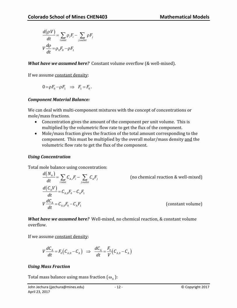
Tank Flow — Chemical Reaction

Let’s assume we have an isothermal, constant volume CSTR with a chemical reaction:

1A Bk The inlet stream has no B in it. The molar balances will be:

A0 A0 0 A 1 A

dCV F C F C k C V

dt

B0 B 1 A

dCV F C k C V

dt

To determine BC t we could first solve for AC t from the first equation & then plug it into the 2nd equation. However, if the reaction is actually

1

2

A Bk

k

then the molar balances will be:

A0 A0 0 A 1 A 2 B

dCV F C F C k C V k C V

dt

B0 B 1 A 2 B

dCV F C k C V k C V

dt



Now the equations are coupled. Some additional manipulation must be done to separate the BC t terms from the AC t terms & visa versa. From the 2nd equation:

0 2BA B

1 1

1 F k VdCC C

k dt k V

and (assuming 0F constant):

2

0 2A B B2

1 1

1 F k VdC d C dC

dt k dt k V dt

Substituting these expressions into the 1st equation gives an expression in just BC , not AC :

20 2 0 2B B B

0 A0 0 1 B 2 B21 1 1 1

1 1F k V F k Vd C dC dCV F C F k V C k C V

k dt k V dt k dt k V

2

0 1 0 20 2 0 1B B B0 A0 B 2 B2

1 1 1 1

F k V F k VF k V F k Vd C dC dCVF C C k C V

k dt k dt k dt k V

20 1 0 20 1 2B B

2 B 0 A021 1 1

2 F k V F k VF k V k Vd C dCVk V C q C

k dt k dt k V

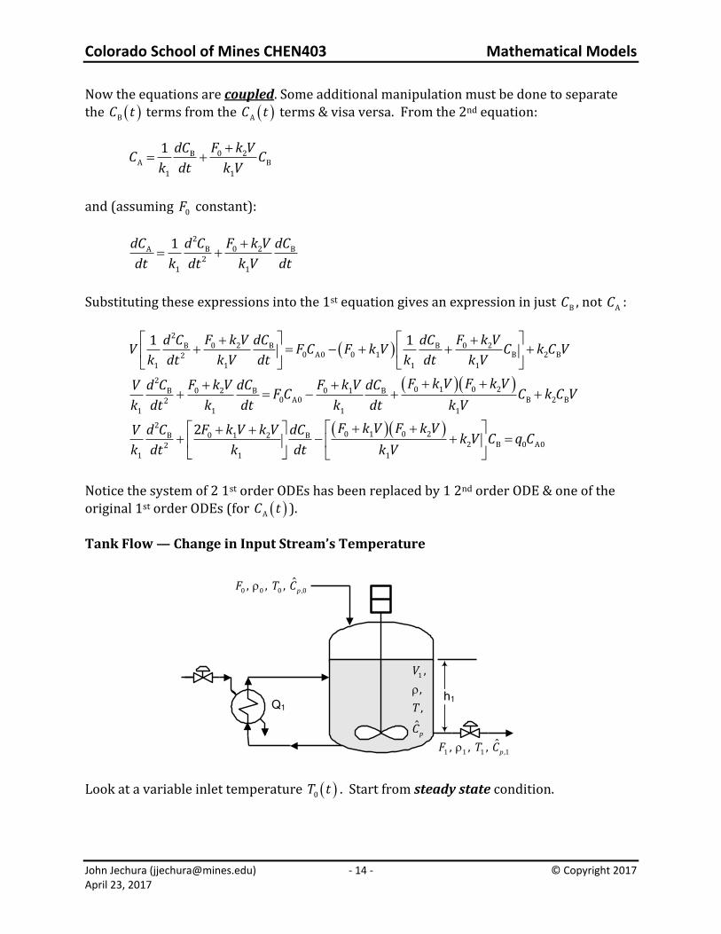
Notice the system of 2 1st order ODEs has been replaced by 1 2nd order ODE & one of the original 1st order ODEs (for AC t ). Tank Flow — Change in Input Stream’s Temperature

Q1

h1

1 1 1 ,1ˆ, , , pF T C

0 0 0 ,0ˆ, , , pF T C

1 ,

,

,

ˆp

V

T

C

Look at a variable inlet temperature 0T t . Start from steady state condition.



State Variables:

• Densities • Temperatures

• Flow rates Initial state:

Steady State total mass balance:

: :


d VF F

dt (well-mixed)

0 0 1 10 F F (steady state)

Note that this also implies that 0 0 1 1 0F F w for any ( )T . Steady state energy balance:

: :

ˆˆ ˆ

i i i j si inlet j outlet

d HVF H F H Q W

dt (well-mixed)

0 0 0 1 1 1 1ˆ ˆ0 F H F H Q (steady state)

0 0 0 0 0 1 1 1 1

ˆ ˆˆ ˆ0 p ref ref p ref refm C T T H m C T T H Q

0 0 1 1ˆ0 pm C T T Q (constant heat capacity & reference enthalpy)

11 0

0ˆ

p

QT T

m C

Transient solutions

After change, total mass balance:

1

0 0 1 1 0 1

d VF F m m

dt (well-mixed)

What does this assume? Well mixed. Energy balance:

1 1

0 0 0 1 1 1 1

ˆˆ ˆ

d VHF H F H Q

dt (well-mixed)



1 1

1 1 0 0 0 1 1 1 1

ˆˆ ˆ ˆd V dH

H V F H F H Qdt dt

(chain rule)

1 1 1

1 1 0 0 0 1 1 1 1

1

ˆˆ ˆ ˆd V dH dT

H V F H F H Qdt dT dt

(chain rule)

1 1

1 1 0 0 0 1 1 1 1ˆˆ ˆ ˆ

p

d V dTH VC F H F H Q

dt dt (definition of heat capacity)

1 1

1 1 0 0 1 1 1ˆˆ ˆ ˆ

p

d V dTH VC m H m H Q

dt dt

11 0 1 1 0 0 1 1 1

ˆˆ ˆ ˆp

dTH m m VC m H m H Q

dt (derivative from mass balance)

11 0 0 1 1

ˆ ˆ ˆp

dTVC m H H Q

dt (mathematical manipulation)

Note that this expression does not depend upon assumptions of constant volume or constant density!

11 0 0 1 1

ˆ ˆp p

dTVC m C T T Q

dt (constant ˆ

pC & reference state)

Can do some additional math. We could normalize the form of the ODE so that the coefficient on the time derivative is 1; in this class, however, we will normally want the

coefficient on the variable without the derivative to be 1:

1 1 10 1

0 0ˆ

p

V dT QT T

m dt m C

1 1 11 0

0 0

ˆ

ˆ ˆp

p p

VC dT QT T

dtm C m C

Notice that the term 1 0/V m has units of time. This can be thought of as a characteristic time constant for the system. Note — Even though the derivation of the ODE does not depend upon whether the system has constant volume and/or density, the integration with time will depend upon this! What if the heat input is described by Newton’s law?

Let’s assume 1 sQ UA T T . Then the ODE becomes:

11 0 0 1

ˆ ˆp p s

dTVC m C T T UA T T

dt



11 0 0 0 1

ˆ ˆ ˆp p s p

dTVC m C T UAT m C UA T

dt

1 011 0

0 0 0

ˆ ˆ

ˆ ˆ ˆp p

s

p p p

VC m CdT UAT T T

dtm C UA m C UA m C UA

.

The form of the solution is the same, but the characteristic time constant is now

1 0ˆ ˆ/p pVC m C UA & is dependent upon heating parameters.

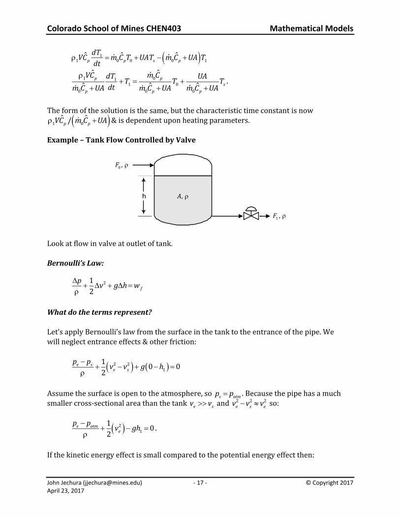
Example – Tank Flow Controlled by Valve

h

1 , F

0 , F

, A

Look at flow in valve at outlet of tank. Bernoulli’s Law:

21

2f

pv g h w

What do the terms represent? Let’s apply Bernoulli’s law from the surface in the tank to the entrance of the pipe. We will neglect entrance effects & other friction:

2 21

10 0

2e s

e s

p pv v g h

Assume the surface is open to the atmosphere, so s atmp p . Because the pipe has a much smaller cross-sectional area than the tank e sv v and 2 2 2

e s ev v v so:

21

10

2e atm

e

p pv gh

.

If the kinetic energy effect is small compared to the potential energy effect then:



21 1 1

10

2e atm e atm

e e atm

p p p pv gh gh p p gh

.

It is normally assumed that at the valve outlet the kinetic energy effect is what creates

the pressure drop, so:

2 2 2 2 21 1

02 2

e vv e v ev e v v

p pp p p pv v v v

If v atmp p , then:

21 1

22 2e atm

v v

p pv gh v gh

The flow rate through a valve is v v vF A v which means that:

1 12v v vF A gh C h where 2v vC A g .

Opening and closing the valve will change vA and hence vC . Total mass balance reduces to volume balance for constant density:

0 1 0 1

d V dVF F F F

dt dt

0 v

dhA F C h

dt

This is a non-linear ODE. Sometimes we can get an analytical solution for this particular ODE. For example, for a step change in flow such that 0inF t F from *

0F :

0 0

0

h t

hv

Adh dt

F C h

0

2

0

y

yv

Ad y t

F C y

00

2y

yv

Aydy t

F C y

0

002

2 ln

y

v

v v y

FyA F C y t

C C



0 0 02

0 0

2 ln v

v v v

y y F F C yA t

C C F C y

0 0 02

0 0

2 ln v

v v v

h h F F C hA t

C C F C h

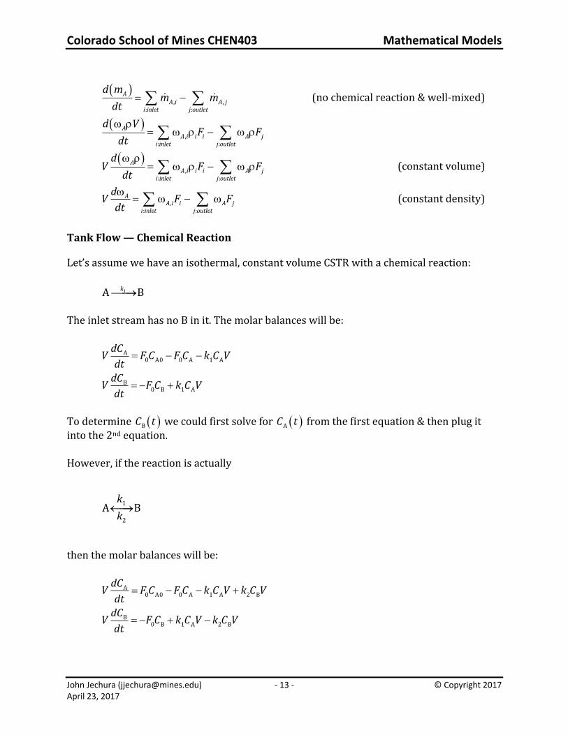
If the inlet flow is more complicated or if this equation is part of a larger set of equations, there is no guarantee that an analytical solution exists. Example: Chemical Reaction

F0

F1

Tcoil

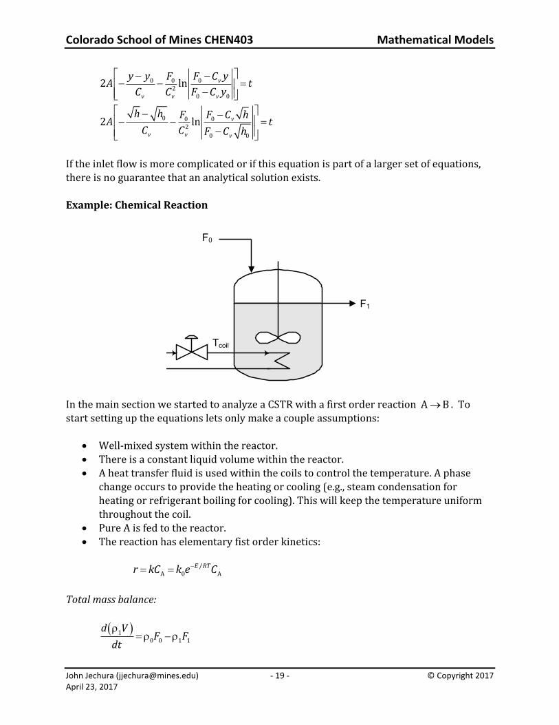
In the main section we started to analyze a CSTR with a first order reaction A B . To start setting up the equations lets only make a couple assumptions:

• Well-mixed system within the reactor. • There is a constant liquid volume within the reactor.

• A heat transfer fluid is used within the coils to control the temperature. A phase change occurs to provide the heating or cooling (e.g., steam condensation for heating or refrigerant boiling for cooling). This will keep the temperature uniform throughout the coil.

• Pure A is fed to the reactor. • The reaction has elementary fist order kinetics:

/A 0 A

E RTr kC k e C

Total mass balance:

1

0 0 1 1

d VF F

dt



10 0 1 1 0 1

dV F F m m

dt (Constant volume)

Mole balance on A:

A1A

A0 0 A1 1

d C VdNC F C F rV

dt dt

1/A1

A0 0 A1 1 0 A1

E RTdCV C F C F k e C V

dt (Kinetic expression)

Mole balance on B:

B1B

B1 1

d C VdNC F rV

dt dt

1/B1

B1 1 0 A1

E RTdCV C F k e C V

dt (Kinetic expression)

Energy balance:

1 1

0 0 0 1 1 1 1

ˆˆ ˆ

coil

d VHF H F H UA T T

dt

1 1

0 0 0 1 1 1 1

ˆˆ ˆ

coil

d HV F H F H UA T T

dt (Constant volume)

1 11 1 0 0 0 1 1 1 1

ˆˆ ˆ ˆ

coil

dH dV H V F H F H UA T T

dt dt (Chain rule)

11 1 0 0 1 1 0 0 0 1 1 1 1

ˆˆ ˆ ˆ

coil

dHV H F F F H F H UA T T

dt (Mass balance)

11 0 0 1 0 0 0 1

ˆˆ ˆ

coil

dHV F H F H UA T T

dt (Cancel like terms)

11 0 0 0 1 1

ˆˆ ˆ

coil

dHV F H H UA T T

dt (A little algebra)



11 1 0 0 0 1 1

ˆ ˆ ˆp coil

dTVC F H H UA T T

dt (Chain rule & ˆ

pC definition)

This energy balance equation is general and has the same form whether there is a heat of reaction or not. So, where is the heat of reaction? (Or heats of mixing, or temperature dependent heat capacities, or composition dependent heat capacities for that matter.) It was noted before that the heat of reaction is embedded in the difference in the enthalpies,

0 1ˆ ˆH H ; this is all well and good to say, but it doesn’t really help in the practical matter of

setting up the energy balance equation to relate all of the relevant temperatures. To simplify the math, let’s make two other assumptions:

• The heat capacity is constant with respect to temperature (though not necessarily with respect to composition).

• The enthalpies mix ideally (i.e., no heat of mixing effects). With these assumptions the enthalpies can be expressed as:

0 0 0 0ˆˆ ˆ

p ref refH C T T H

1 1 1 1ˆˆ ˆ

p ref refH C T T H

and the energy balance is:

11 1 0 0 0 0 0 1 1 1 1

ˆ ˆ ˆˆ ˆp p ref ref p ref ref coil

dTVC F C T T H C T T H UA T T

dt

11 1 0 0 0 0 1 1 0 0 0 1 1

ˆ ˆ ˆ ˆ ˆp p ref p ref ref ref coil

dTVC F C T T C T T F H H UA T T

dt.

The heat of reaction is still embedded in the term relating the specific enthalpy values at the reference conditions of temperature ( refT ) and composition. Notice that assuming the heat capacity is not composition dependent does not affect this reference state term, it only simplifies the first term relating the net flow of enthalpy to the system; if we assume no composition dependency then 0 1

ˆ ˆ ˆp p pC C C and:

11 0 0 0 1 0 0 0 1 1

ˆ ˆ ˆ ˆ ˆp p ref p ref ref ref coil

dTVC F C T T C T T F H H UA T T

dt

11 0 0 0 1 0 0 0 1 1

ˆ ˆ ˆ ˆp p ref ref coil

dTVC F C T T F H H UA T T

dt.



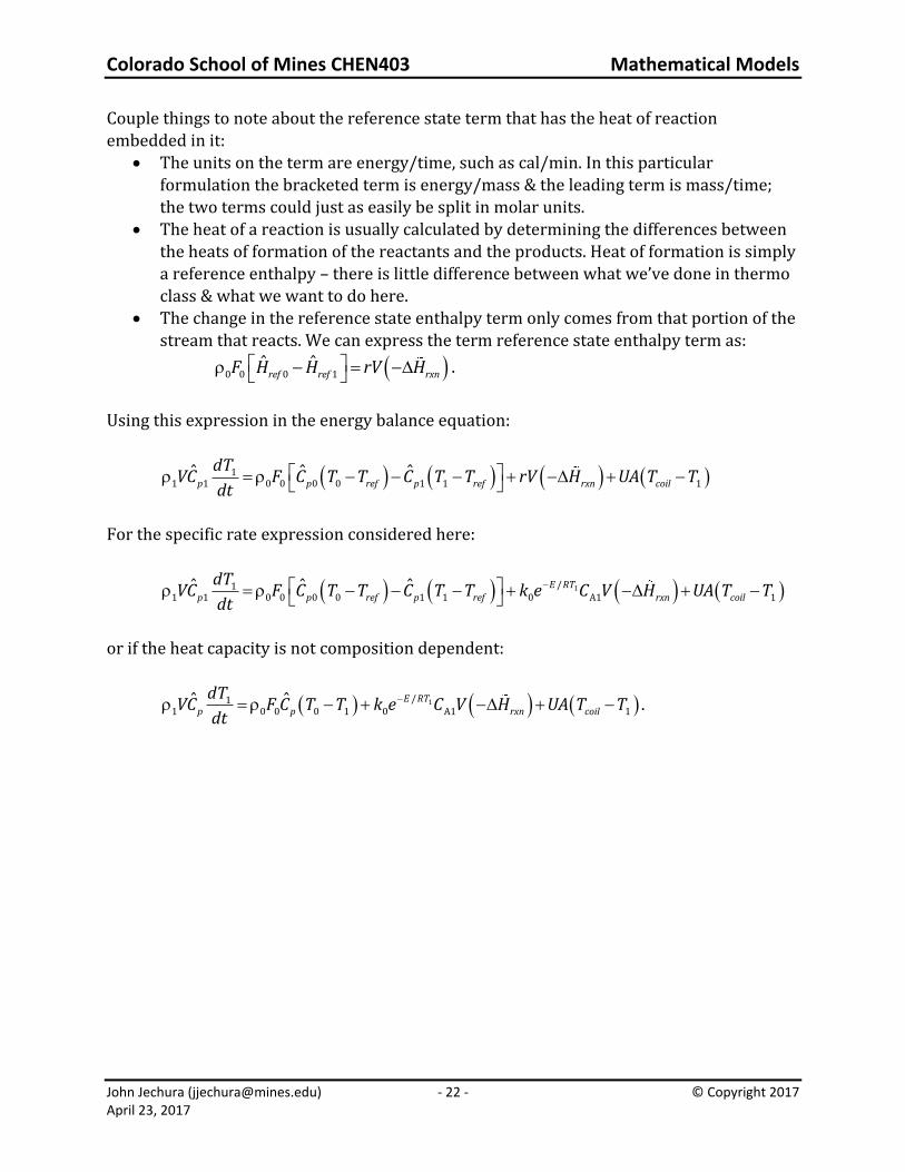
Couple things to note about the reference state term that has the heat of reaction embedded in it:

• The units on the term are energy/time, such as cal/min. In this particular formulation the bracketed term is energy/mass & the leading term is mass/time;

the two terms could just as easily be split in molar units. • The heat of a reaction is usually calculated by determining the differences between

the heats of formation of the reactants and the products. Heat of formation is simply a reference enthalpy – there is little difference between what we’ve done in thermo class & what we want to do here.

• The change in the reference state enthalpy term only comes from that portion of the stream that reacts. We can express the term reference state enthalpy term as:

0 0 0 1

ˆ ˆref ref rxnF H H rV H .

Using this expression in the energy balance equation:

11 1 0 0 0 0 1 1 1

ˆ ˆ ˆp p ref p ref rxn coil

dTVC F C T T C T T rV H UA T T

dt

For the specific rate expression considered here:

1/11 1 0 0 0 0 1 1 0 A1 1

ˆ ˆ ˆ E RT

p p ref p ref rxn coil

dTVC F C T T C T T k e C V H UA T T

dt

or if the heat capacity is not composition dependent:

1/1

1 0 0 0 1 0 A1 1ˆ ˆ E RT

p p rxn coil

dTVC F C T T k e C V H UA T T

dt.

Documents

Colorado School of Mines CHEN403 Mathematical Models ...inside.mines.edu/~jjechura/ProcessDynamics/02_HeatMaterialBalance... · Setting up the Mathematical Model Review of Heat &