Embed Size (px)
Citation preview
1
The RKHS Approach to Minimum Variance
Estimation Revisited: Variance Bounds,
Sufficient Statistics, and Exponential Families
Alexander Jung, Member, IEEE, Sebastian Schmutzhard, and Franz Hlawatsch, Fellow, IEEE
Abstract—The mathematical theory of reproducing kernelHilbert spaces (RKHS) provides powerful tools for minimumvariance estimation (MVE) problems. Here, we extend theclassical RKHS-based analysis of MVE in several directions. Wedevelop a geometric formulation of five known lower bounds onthe estimator variance (Barankin bound, Cramér–Rao bound,constrained Cramér–Rao bound, Bhattacharyya bound, andHammersley-Chapman-Robbins bound) in terms of orthogonalprojections onto a subspace of the RKHS associated with agiven MVE problem. We show that, under mild conditions,the Barankin bound (the tightest possible lower bound on theestimator variance) is a lower semi-continuous function of theparameter vector. We also show that the RKHS associated with anMVE problem remains unchanged if the observation is replacedby a sufficient statistic. Finally, for MVE problems conformingto an exponential family of distributions, we derive novel closed-form lower bounds on the estimator variance and show that areduction of the parameter set leaves the minimum achievablevariance unchanged.
Index Terms—Minimum variance estimation, exponentialfamily, reproducing kernel Hilbert space, RKHS, Cramér–Rao bound, Barankin bound, Hammersley–Chapman–Robbinsbound, Bhattacharyya bound, locally minimum variance unbi-ased estimator.
I. INTRODUCTION
We consider the problem of estimating the value g(x) of a
known deterministic function g(·) evaluated at an unknown
nonrandom parameter vector x ∈ X , where the parameter
set X is known. The estimation of g(x) is based on an
observed vector y, which is modeled as a random vector
with an associated probability measure [1] µyx or, as a special
case, an associated probability density function (pdf) f(y;x),both parametrized by x ∈ X . More specifically, we study the
problem of minimum variance estimation (MVE), where one
aims at finding estimators with minimum variance under the
constraint of a prescribed bias. Our treatment of MVE will
A. Jung and F. Hlawatsch are with the Institute of Telecommunica-tions, Vienna University of Technology, A-1040 Vienna, Austria (e-mail:{ajung,fhlawats}@nt.tuwien.ac.at). S. Schmutzhard is with the NumericalHarmonic Analysis Group, Faculty of Mathematics, University of Vienna,A-1090 Vienna, Austria (e-mail: [email protected]). Thiswork was supported in part by the Austrian Science Fund under GrantsS10602-N13 and S10603-N13 within the National Research Network Signaland Information Processing in Science and Engineering and in part by theWiener Wissenschafts-, Forschungs- und Technologiefonds (WWTF) underGrant MA 07-004.
Copyright (c) 2014 IEEE. Personal use of this material is permitted.However, permission to use this material for any other purposes must beobtained from the IEEE by sending a request to [email protected].
be based on the mathematical framework and methodology of
reproducing kernel Hilbert spaces (RKHS).
A. State of the Art and Motivation
The RKHS approach to MVE was introduced in the seminal
papers [2] and [3]. On a general level, the theory of RKHS
yields efficient methods for high-dimensional optimization
problems. These methods are popular, e.g., in machine learn-
ing [4], [5]. For the MVE problem considered here, the
optimization problem is the minimization of the estimator
variance subject to a bias constraint. The RKHS approach to
MVE enables a consistent and intuitive geometric treatment
of the MVE problem. In particular, the determination of
the minimum achievable variance (or Barankin bound) and
of the locally minimum variance estimator reduces to the
calculation of the squared norm and isometric image of a
specific vector—representing the prescribed estimator bias—
that belongs to the RKHS associated with the estimation
problem. This reformulation is interesting from a theoretical
perspective; in addition, it may also be the basis for an efficient
computational evaluation. Furthermore, a wide class of lower
bounds on the minimum achievable variance (and, in turn,
on the variance of any estimator) is obtained by performing
projections onto subspaces of the RKHS. Again, this enables
an efficient computational evaluation of these bounds.
A specialization to estimation problems involving sparsity
constraints was presented in [6]–[8]. For certain special cases
of these sparse estimation problems, the RKHS approach al-
lows the derivation of closed-form expressions of the minimum
achievable variance and the corresponding locally minimum
variance estimators. The RKHS approach has also proven to
be a valuable tool for the analysis of estimation problems
involving continuous-time random processes [2], [3], [9].
B. Contribution and Outline
The main contributions of this paper concern an RKHS-
theoretic analysis of the performance of MVE, with a focus
on lower variance bounds, sufficient statistics, and observa-
tions conforming to an exponential family of distributions.
First, we give a geometric interpretation of some well-known
lower bounds on the estimator variance. The tightest of these
bounds, i.e., the Barankin bound, is proven to be a lower
semi-continuous function of the parameter vector x under
mild conditions. We then analyze the role of a sufficient
Copyright 2014 IEEE IEEE Trans. Inf. Theory, vol. 60, no. 7, July 2014, pp. 4050–4065
2
statistic from the RKHS viewpoint. In particular, we prove
that the RKHS associated with an estimation problem re-
mains unchanged if the observation y is replaced by any
sufficient statistic. Furthermore, we characterize the RKHS
for estimation problems with observations conforming to an
exponential family of distributions. It is found that this RKHS
has a strong structural property, and that it is explicitly related
to the moment-generating function of the exponential family.
Inspired by this relation, we derive novel lower bounds on the
estimator variance, and we analyze the effect of parameter set
reductions. The lower bounds have a particularly simple form.
The remainder of this paper is organized as follows. In
Section II, basic elements of MVE are reviewed and the
RKHS approach to MVE is summarized. In Section III, we
present an RKHS-based geometric interpretation of known
variance bounds and demonstrate the lower semi-continuity of
the Barankin bound. The effect of replacing the observation
by a sufficient statistic is studied in Section IV. In Section V,
the RKHS for exponential family-based estimation problems
is investigated, novel lower bounds on the estimator variance
are derived, and the effect of a parameter set reduction is
analyzed. We note that the proofs of most of the new results
presented can be found in the doctoral dissertation [10] and
will be referenced in each case.
C. Notation and Basic Definitions
We will use the shorthand notations N , {1, 2, 3, . . .},
Z+ , {0, 1, 2, . . .}, and [N ] , {1, 2, . . . , N}. The open ball
in RN with radius r > 0 and centered at xc is defined as
B(xc, r) ,{
x∈RN∣
∣‖x−xc‖2< r}
. We call x ∈ X ⊆ RN
an interior point if B(x, r) ⊆ X for some r>0. The set of all
interior points of X is called the interior of X and denoted
X o. A set X is called open if X = X o.
Boldface lowercase (uppercase) letters denote vectors (ma-
trices). The superscript T stands for transposition. The kth
entry of a vector x and the entry in the kth row and lth column
of a matrix A are denoted by (x)k = xk and (A)k,l = Ak,l,
respectively. The kth unit vector is denoted by ek, and the
identity matrix of size N ×N by IN . The Moore-Penrose
pseudoinverse [11] of a rectangular matrix A ∈ RM×N is
denoted by A†.
A function f(·) : D→R, with D⊆RN, is said to be lower
semi-continuous at x0∈D if for every ε>0 there is a radius
r> 0 such that f(x) ≥ f(x0) − ε for all x ∈ B(x0, r). (This
definition is equivalent to lim infx→x0 f(x) ≥ f(x0), where
lim infx→x0 f(x) , supr>0
{
infx∈D∩ [B(x0,r)\{x0}] f(x)}
[12], [13].) The restriction of a function f(·) : D → R to
a subdomain D′ ⊆ D is denoted by f(·)∣
∣
D′. Given a multi-
index p = (p1 · · · pN )T ∈ ZN+ , we define the partial derivative
of order p of a real-valued function f(·) : D → R, with
D ⊆ RN, as
∂pf(x)∂xp , ∂p1
∂xp1k
· · · ∂pN
∂xpNN
f(x) (if it exists) [13],
[14]. Similarly, for a function f(· , ·) : D × D → R and
two multi-indices p1,p2 ∈ ZN+ , we denote by
∂p1∂p2f(x1,x2)
∂xp11 ∂x
p22
the partial derivative of order (p1,p2), where f(x1,x2) is
considered as a function of the “super-vector” (xT1 xT
2 )T of
length 2N . Given a vector-valued function φ(·) : RM → RN
and p ∈ ZN+ , we denote the product
∏Nk=1
(
φk(y))pk
by
φp(y).The probability measure of a random vector y taking on
values in RM is denoted by µy [1], [15]–[17]. We consider
probability measures that are defined on the measure space
given by all M -dimensional Borel sets on RM [1, Sec. 10].
The probability measure assigns to a measureable set A ⊆ RM
the probability
P{y ∈ A} ,
∫
RM
IA(y′) dµy(y′) =
∫
A
dµy(y′) ,
where IA(·) : RM → {0, 1} denotes the indicator function
of the set A. We will also consider a family of probability
measures {µyx}x∈X parametrized by a nonrandom parameter
vector x ∈ X . We assume that there exists a dominating
measure µE , so that we can define the pdf f(y;x) (again
parametrized by x) as the Radon-Nikodym derivative of the
measure µyx with respect to the measure µE [1], [15]–[17].
(In general, we will choose for µE the Lebesgue measure
on RM.) We refer to both the set of measures {µy
x}x∈X
and the set of pdfs {f(y;x)}x∈X as the statistical model.
Given a (possibly vector-valued) deterministic function t(y),the expectation operation is defined by [1]
Ex{t(y)} ,
∫
RM
t(y′) dµyx(y
′) =
∫
RM
t(y′) f(y′;x) dy′,
where the subscript in Ex indicates the dependence on the
parameter vector x parametrizing µyx(y) and f(y;x).
II. FUNDAMENTALS
A. Review of MVE
It will be convenient to denote a classical (frequentist)
estimation problem by the triple E =(
X , f(y;x),g(·))
,
consisting of the parameter set X ⊆ RN, the statistical model
{f(y;x)}x∈X , with y ∈ RM, and the parameter function
g(·) : X → RP . Note that our setting includes estimation
of the parameter vector x itself, which is obtained when
g(x) = x. The result of estimating g(x) from y is an estimate
g ∈ RP, which is derived from y via a deterministic estimator
g(·) : RM → RP, i.e., g = g(y). We assume that any estimator
is a measurable mapping from RM to R
P [1, Sec. 13]. A
convenient characterization of the performance of an estimator
g(·) is the mean squared error (MSE) defined as
ε , Ex
{
‖g(y)− g(x)‖22}
=
∫
RM
‖g(y)− g(x)‖22 f(y;x) dy.
We will write ε(g(·);x) to explicitly indicate the dependence
of the MSE on the estimator g(·) and the parameter vector
x. Unfortunately, for a general estimation problem E =(
X , f(y;x),g(·))
, there does not exist an estimator g(·) that
minimizes the MSE simultaneously for all parameter vectors
x ∈ X [18], [19]. This follows from the fact that minimizing
the MSE at a given parameter vector x0 always yields zero
MSE; this is achieved by the estimator g0(y) = g(x0), which
completely ignores the observation y.
A popular rationale for the design of good estimators is
MVE. This approach is based on the MSE decomposition
ε(g(·);x) = ‖b(g(·);x)‖22 + v(g(·);x) , (1)
3
with the estimator bias b(g(·);x) , Ex{g(y)}−g(x) and the
estimator variance v(g(·);x) , Ex
{
‖g(y) − Ex{g(y)}‖22
}
.
In MVE, one fixes the bias for all parameter vectors, i.e.,
b(g(·);x)!= c(x) for all x ∈ X , with a prescribed bias
function c(·) : X → RP, and considers only estimators with
the given bias. Note that fixing the estimator bias is equivalent
to fixing the estimator mean, i.e., Ex
{
g(y)} != γ(x) for all
x∈X , with the prescribed mean function γ(x) , c(x)+g(x).The important special case of unbiased estimation is obtained
for c(x) ≡ 0 or equivalently γ(x) ≡ g(x) for all x ∈ X .
Fixing the bias can be viewed as a kind of regularization of
the set of considered estimators [15], [19], because useless
estimators like the estimator g0(y) = g(x0) are excluded.
Another justification for fixing the bias is the fact that, if a
large number of independent and identically distributed (i.i.d.)
realizations {yi}Li=1 of the vector y are observed, then, under
certain technical conditions, the bias term dominates in the
decomposition (1). Thus, in that case, the MSE is small if and
only if the bias is small; this means that the estimator has to
be effectively unbiased, i.e., b(g(·);x) ≈ 0 for all x∈X .
For a fixed “reference” parameter vector x0 ∈ X and a
prescribed bias function c(·), we define the set of allowed
estimators by
A(c(·),x0)
,{
g(·)∣
∣ v(g(·);x0) < ∞ , b(g(·);x) = c(x) ∀x∈X}
.
We call a bias function c(·) valid for the estimation problem
E = (X , f(y;x),g(·)) at x0 ∈ X if the set A(c(·),x0) is
nonempty. This means that there is at least one estimator g(·)with finite variance at x0 and whose bias equals c(·), i.e.,
b(g(·);x) = c(x) for all x∈X . From (1), it follows that for a
fixed bias c(·), minimizing the MSE ε(g(·);x0) is equivalent
to minimizing the variance v(g(·);x0). Therefore, in MVE,
one attempts to find estimators that minimize the variance
under the constraint of a prescribed bias function c(·). Let
M(c(·),x0) , infg(·)∈A(c(·),x0)
v(g(·);x0) (2)
denote the minimum (strictly speaking, infimum) variance at
x0 for bias function c(·). If A(c(·),x0) is empty, i.e., if c(·) is
not valid, we set M(c(·),x0) , ∞. Any estimator g(x0)(·) ∈A(c(·),x0) that achieves the infimum in (2), i.e., for which
v(
g(x0)(·);x0
)
= M(c(·),x0), is called a locally minimum
variance (LMV) estimator at x0 for bias function c(·) [2],
[3], [15]. The corresponding minimum variance M(c(·),x0) is
called the minimum achievable variance at x0 for bias function
c(·). The minimization problem (2) is referred to as a minimum
variance problem (MVP). By its definition in (2), M(c(·),x0)is a lower bound on the variance at x0 of any estimator with
bias function c(·), i.e.,
g(·) ∈ A(c(·),x0) ⇒ v(g(·);x0) ≥ M(c(·),x0) . (3)
In fact, M(c(·),x0) is the tightest lower bound, which is
sometimes referred to as the Barankin bound.
If, for a prescribed bias function c(·), there exists an
estimator that is the LMV estimator simultaneously at all
x0 ∈ X , then that estimator is called the uniformly minimum
variance (UMV) estimator for bias function c(·) [2], [3], [15].
For many estimation problems, a UMV estimator does not
exist. However, it always exists if there exists a complete
sufficient statistic [15, Theorem 1.11 and Corollary 1.12], [20,
Theorem 6.2.25]. Under mild conditions, this includes the
case where the statistical model corresponds to an exponential
family.
The variance to be minimized can be decomposed as
v(g(·);x0) =∑
l∈[P ]
v(gl(·);x0) ,
where gl(·) ,(
g(·))
land v(gl(·);x0) , Ex0
{[
gl(y) −
Ex0{gl(y)}]2}
for l ∈ [P ]. Moreover, g(·) ∈ A(c(·),x0)if and only if gl(·) ∈ A(cl(·),x0) for all l ∈ [P ], where
cl(·) ,(
c(·))
l. It follows that the minimization of v(g(·);x0)
in (2) can be reduced to P separate problems of minimizing
the component variances v(gl(·);x0), each involving the op-
timization of a single scalar component gl(·) of g(·) subject
to the scalar bias constraint b(gl(·);x) = cl(x) for all x∈X .
Therefore, without loss of generality, we will hereafter assume
that the parameter function g(x) is scalar-valued, i.e., P =1.
B. Review of the RKHS Approach to MVE
A powerful mathematical toolbox for MVE is provided by
RKHS theory [2], [3], [21]. In this subsection, we review basic
definitions and results of RKHS theory and its application to
MVE, and we discuss a differentiability property that will be
relevant to the variance bounds considered in Section III.
An RKHS is associated with a kernel function, which is a
function R(· , ·) : X×X → R with the following two properties
[21]:
• It is symmetric, i.e., R(x1,x2) = R(x2,x1) for all
x1,x2 ∈ X ;
• for every finite set {x1, . . . ,xD} ⊆ X , the matrix
R ∈ RD×D with entries Rm,n = R(xm,xn) is positive
semidefinite.
There exists an RKHS for any kernel function R(· , ·) : X×X→ R [21]. This RKHS, denoted H(R), is a Hilbert space
equipped with an inner product 〈· , ·〉H(R) such that, for any
x∈X ,
• R(·,x) ∈ H(R) (here, R(·,x) denotes the function
fx(x′) = R(x′,x) with a fixed x ∈ X );
• for any function f(·) ∈H(R),⟨
f(·), R(· ,x)⟩
H(R)= f(x) . (4)
Relation (4), which is known as the reproducing property,
defines the inner product 〈f, g〉H(R) for all f(·), g(·) ∈ H(R)because (in a certain sense) any f(·) ∈ H(R) can be ex-
panded into the set of functions {R(·,x)}x∈X . In particular,
consider two functions f(·), g(·) ∈ H(R) that are given as
f(·) =∑
xk∈D akR(·,xk) and g(·) =∑
x′
l∈D′ blR(·,x′
l) with
coefficients ak, bl ∈ R and (possibly infinite) sets D,D′ ⊆ X .
Then, by the linearity of inner products and (4),⟨
f(·), g(·)⟩
H(R)=∑
xk∈D
∑
x′
l∈D′
akblR(xk,x′l) .
4
1) The RKHS Associated with an MVP: Consider the
class of MVPs that is defined by an estimation problem
E =(
X , f(y;x), g(·))
, a reference parameter vector x0 ∈X ,
and all possible prescribed bias functions c(·) : X → R.
With this class of MVPs, we can associate a kernel function
RE,x0(· , ·) : X × X → R and, in turn, an RKHS H(RE,x0)[2], [3]. (Note that, as our notation indicates, RE,x0(· , ·) and
H(RE,x0) depend on E and x0 but not on g(·) or c(·).) We
assume that
P{f(y;x0) 6= 0} = 1 , (5)
where the probability is evaluated for some underlying dom-
inating measure µE . We can then define the likelihood ratio
as
ρE,x0(y,x) ,
f(y;x)
f(y;x0), if f(y;x0) 6= 0
0 , else.
(6)
We consider ρE,x0(y,x) as a random variable (since it is
a function of the random vector y) that is parametrized by
x ∈ X . Furthermore, we define the Hilbert space LE,x0 as
the closure of the linear span1 of the set of random variables{
ρE,x0(y,x)}
x∈X. The topology of LE,x0 is determined by
the inner product 〈· , ·〉RV : LE,x0 × LE,x0 → R defined by⟨
ρE,x0(y,x1), ρE,x0(y,x2)⟩
RV
, Ex0
{
ρE,x0(y,x1) ρE,x0(y,x2)}
. (7)
It can be shown that it is sufficient to define the inner product
only for the random variables{
ρE,x0(y,x)}
x∈X[2]. We will
assume that⟨
ρE,x0(y,x1), ρE,x0(y,x2)⟩
RV< ∞ , for all x1,x2 ∈ X .
(8)
The assumptions (5) and (8) (or variants thereof) are standard
in the literature on MVE [2], [3], [23], [24]. They are typi-
cally satisfied for the important and large class of estimation
problems arising from exponential families (cf. Section V).
The inner product 〈· , ·〉RV : LE,x0×LE,x0 → R can now be
interpreted as a kernel function RE,x0(· , ·) : X×X → R:
RE,x0(x1,x2) ,⟨
ρE,x0(y,x1), ρE,x0(y,x2)⟩
RV. (9)
The RKHS induced by RE,x0(· , ·) will be denoted by HE,x0 ,
i.e., HE,x0 , H(RE,x0). This is the RKHS associated with
the estimation problem E =(
X , f(y;x), g(·))
and the corre-
sponding class of MVPs at x0 ∈ X . (Note that RE,x0(· , ·) and
HE,x0 do not depend on g(·).)Assumption (5) implies that the likelihood ratio ρE,x0(y,x)
is measurable with respect to the underlying dominating
measure µE . Furthermore, ρE,x0(y,x) is the Radon-Nikodym
derivative [1], [16] of the probability measure µyx induced by
f(y;x) with respect to the probability measure µyx0
induced
by f(y;x0) (cf. [1], [22], [25]). It is important to observe
that ρE,x0(y,x) does not depend on the dominating measure
µE underlying the definition of the pdfs f(y;x). Thus, the
kernel RE,x0(· , ·) given by (9) does not depend on µE either.
1A detailed discussion of the concepts of closure, inner product, orthonor-mal basis, and linear span in the context of abstract Hilbert space theory canbe found in [2] and [22].
Moreover, under assumption (5), there exists the Radon-
Nikodym derivative of µyx with respect to µy
x0. This implies,
trivially, that µyx is absolutely continuous with respect to µy
x0,
or, equivalently, that µyx0
dominates the measures {µyx}x∈X [1,
p. 443]. Therefore, we can use the measure µyx0
as the base
measure µE for the estimation problem E .
The two Hilbert spaces LE,x0 and HE,x0 are isometric. In
fact, as proven in [2], a specific congruence (i.e., isometric
mapping of functions in HE,x0 to functions in LE,x0 ) J[·] :HE,x0 → LE,x0 is given by
J[RE,x0(·,x)] = ρE,x0(·,x) .
The isometry J[f(·)] can be evaluated for an arbitrary func-
tion f(·) ∈ HE,x0 by expanding f(·) into the elementary
functions {RE,x0(·,x)}x∈X (cf. [2]). Given the expansion
f(·) =∑
xk∈D akRE,x0(·,xk) with coefficients ak ∈ R and a
(possibly infinite) set D ⊆ X , the isometric image of f(·) is
obtained as J[f(·)] =∑
xk∈D ak ρE,x0(·,xk).
2) RKHS-based Analysis of MVE: An RKHS-based anal-
ysis of MVE is enabled by the following central result.
Consider an estimation problem E =(
X , f(y;x), g(·))
, a
fixed reference parameter vector x0 ∈ X , and a prescribed
bias function c(·) : X → R, corresponding to the prescribed
mean function γ(·) , c(·) + g(·). Then, as shown in [2] and
[3], the following holds:
• The bias function c(·) is valid for E at x0 if and only if
γ(·) belongs to the RKHS HE,x0 , i.e.,
A(c(·),x0) 6= ∅ ⇐⇒ γ(·) ∈ HE,x0 . (10)
• If the bias function c(·) is valid, the corresponding
minimum achievable variance at x0 is given by
M(c(·),x0) = ‖γ(·)‖2HE,x0− γ2(x0) , (11)
and the LMV estimator at x0 is given by
g(x0)(·) = J[γ(·)] . (12)
This result shows that the RKHS HE,x0 is equal to the set
of the mean functions γ(x) = Ex{g(y)} of all estimators g(·)with a finite variance at x0, i.e., v(g(·);x0) < ∞. Furthermore,
the problem of solving the MVP (2) can be reduced to
the computation of the squared norm ‖γ(·)‖2HE,x0and the
isometric image J[γ(·)] of the prescribed mean function γ(·),viewed as an element of the RKHS HE,x0 . This is especially
helpful if a simple characterization of HE,x0 is available. Here,
following the terminology of [3], what is meant by “simple
characterization” is the availability of an orthonormal basis
(ONB) for HE,x0 such that the inner products of γ(·) with the
ONB functions can be computed easily.
If such an ONB of HE,x0 cannot be found, the relation
(11) can still be used to derive lower bounds on the minimum
achievable variance M(c(·),x0). Indeed, because of (11),
any lower bound on ‖γ(·)‖2HE,x0induces a lower bound on
M(c(·),x0). A large class of lower bounds on ‖γ(·)‖2HE,x0can
be obtained via projections of γ(·) onto a subspace U ⊆ HE,x0 .
Denoting the orthogonal projection of γ(·) onto U by γU (·),
5
we have ‖γU(·)‖2HE,x0
≤ ‖γ(·)‖2HE,x0[22, Chapter 4] and thus,
from (11),
M(c(·),x0) ≥ ‖γU(·)‖2HE,x0
− γ2(x0) , (13)
for an arbitrary subspace U ⊆ HE,x0 . In particular, let us
consider the special case of a finite-dimensional subspace U ⊆HE,x0 that is spanned by a given set of functions ul(·) ∈HE,x0 , i.e.,
U = span{ul(·)}l∈[L] ,
{
f(·) =∑
l∈[L]
alul(·)
∣
∣
∣
∣
∣
al∈ R
}
.
(14)
Here, ‖γU(·)‖2HE,x0
can be evaluated very easily due to the
following expression [10, Theorem 3.1.8]:
‖γU (·)‖2HE,x0
= γTG†γ , (15)
where the vector γ ∈ RL and the matrix G ∈R
L×L are given
elementwise by
γl = 〈γ(·), ul(·)〉HE,x0, Gl,l′ = 〈ul(·), ul′(·)〉HE,x0
. (16)
If all ul(·) are linearly independent, then a larger number Lof basis functions ul(·) entails a higher dimension of U and,
thus, a larger ‖γU (·)‖2HE,x0
; this implies that the lower bound
(13) will be higher (i.e., tighter). In Section III, we will show
that some well-known lower bounds on the estimator variance
are obtained from (13) and (15), using a subspace U of the
form (14) and specific choices for the functions ul(·) spanning
U .
3) Regular Estimation Problems and Differentiable RKHS:
Some of the lower bounds to be considered in Section III
require the estimation problem to satisfy certain regularity
conditions.
Definition II.1. An estimation problem E =(
X , f(y;x), g(·))
satisfying (8) is said to be regular up to order m ∈ N at an
interior point x0 ∈ X o if the following holds:
• For every multi-index p ∈ ZN+ with entries pk ≤ m, the
partial derivatives∂pf(y;x)
∂xp exist and satisfy
Ex0
{(
1
f(y;x0)
∂pf(y;x)
∂xp
)2}
< ∞ ,
for all x ∈ B(x0, r) ,
where r > 0 is a suitably chosen radius such that
B(x0, r) ⊆ X .
• For any function h(·) : RM → R such that Ex{h(y)}
exists, the expectation operation commutes with partial
differentiation in the sense that, for every multi-index p ∈ZN+ with pk ≤m,
∂p
∂xp
∫
RM
h(y) f(y;x) dy
=
∫
RM
h(y)∂pf(y;x)
∂xpdy, for all x ∈ B(x0, r) , (17)
or equivalently
∂pEx{h(y)}
∂xp= Ex
{
h(y)1
f(y;x)
∂pf(y;x)
∂xp
}
,
for all x ∈ B(x0, r) , (18)
provided that the right hand side of (17) and (18) is finite.
• For every pair of multi-indices p1,p2 ∈ ZN+ with p1,k ≤
m and p2,k ≤m, the expectation
Ex0
{
1
f2(y;x0)
∂p1f(y;x1)
∂xp1
1
∂p2f(y;x2)
∂xp2
2
}
depends continuously on the parameter vectors x1,x2 ∈B(x0, r).
We remark that the notion of a regular estimation problem
according to Definition II.1 is somewhat similar to the notion
of a regular statistical experiment introduced in [17, Section
I.7].
The RKHS HE,x0 associated with a regular estimation
problem E has an important structural property, which we
will term differentiable. More precisely, we call an RKHS
H(R) differentiable up to order m if it is associated with
a kernel R(· , ·) : X × X → R that is differentiable up to a
given order m. The properties of differentiable RKHSs have
been previously studied, e.g., in [26]–[28]. As shown in [10,
Theorem 4.4.3], if E is regular up to order m at x0, then HE,x0
is differentiable up to order m.
It will be seen that, under certain conditions, the functions
belonging to an RKHS H(R) that is differentiable up to any
order are characterized completely by their partial derivatives
at any point x0 ∈ X o. This implies via (10) together with
identity (20) below that, for a regular estimation problem, the
mean function γ(x) = Ex{g(y)} of any estimator g(·) with
finite variance at x0 is completely specified by the partial
derivatives{
∂pγ(x)∂xp
∣
∣
x=x0
}
p∈ZN+
(cf. Lemma V.3 in Section
V-D).
Further important properties of a differentiable RKHS have
been reported in [9] and [27]. In particular, for an RKHS H(R)that is differentiable up to order m, and for any x0 ∈ X o and
any p ∈ ZN+ with pk ≤m, the following holds:
• The function r(p)x0 (·) : X →R defined by
r(p)x0(x) ,
∂pR(x,x2)
∂xp2
∣
∣
∣
∣
x2=x0
(19)
is an element of H(R), i.e., r(p)x0 (·) ∈ H(R).
• For any function f(·) ∈ H(R), the partial derivative∂pf(x)∂xp
∣
∣
x=x0exists.
• The inner product of r(p)x0 (·) with an arbitrary function
f(·) ∈ H(R) is given by
⟨
r(p)x0(·), f(·)
⟩
H(R)=
∂pf(x)
∂xp
∣
∣
∣
∣
x=x0
. (20)
Thus, an RKHS H(R) that is differentiable up to order m
contains the functions{
r(p)x0 (x)
}
pk≤m, and the inner products
of any function f(·) ∈ H(R) with the r(p)x0 (x) can be com-
puted easily via differentiation of f(·). This makes function
sets{
r(p)x0 (x)
}
appear as interesting candidates for a simple
characterization of the RKHS H(R). However, in general,
these function sets are not guaranteed to be complete or
6
orthonormal, i.e., they do not generally constitute an ONB. An
important exception is given by certain estimation problems Einvolving an exponential family of distributions, which will be
studied in Section V-D.
Consider an estimation problem E =(
X , f(y;x), g(·))
that
is regular up to order m∈N at x0 ∈X o. According to (10),
the mean function γ(·) of any estimator with finite variance at
x0 belongs to the RKHS HE,x0 . Since E is assumed regular
up to order m, HE,x0 is differentiable up to order m. This, in
turn, implies2 via (10) and (20) that the partial derivatives of
γ(·) at x0 exist up to order m. Therefore, for the derivation
of lower bounds on the minimum achievable variance at x0 in
the case of an estimation problem that is regular up to order mat x0, we can always tacitly assume that the partial derivatives
of γ(·) at x0 exist up to order m; otherwise the corresponding
bias function c(·) = γ(·)− g(·) would not be valid, i.e., there
would not exist any estimator with mean function γ(·) (or,
equivalently, bias function c(·)) and finite variance at x0.
III. RKHS FORMULATION OF KNOWN VARIANCE BOUNDS
Consider an estimation problem E =(
X , f(y;x), g(·))
and
an estimator g(·) with mean function γ(x) = Ex{g(y)} and
bias function c(x) = γ(x) − g(x). We assume that g(·) has
a finite variance at x0, which implies that c(·) is valid and
g(·) ∈ A(c(·),x0); hence, A(c(·),x0) is nonempty. Then,
γ(·) ∈ HE,x0 according to (10). We also recall from our
discussion further above that if the estimation problem Eis regular at x0 up to order m, then the partial derivatives∂pγ(x)∂xp
∣
∣
x=x0exist for all p ∈ Z
N+ with pk ≤m.
In this section, we will demonstrate how five known lower
bounds on the variance—Barankin bound, Cramér–Rao bound,
constrained Cramér–Rao bound, Bhattacharyya bound, and
Hammersley-Chapman-Robbins bound—can be formulated in
a unified manner within the RKHS framework. More specifi-
cally, by combining (3) with (13), it follows that the variance
of g(·) at x0 is lower bounded as
v(g(·);x0) ≥ ‖γU(·)‖2HE,x0
− γ2(x0) , (21)
where U is any subspace of HE,x0 . The five variance bounds
to be considered are obtained via specific choices of U .
A. Barankin Bound
For a (valid) prescribed bias function c(·), the Barankin
bound [23], [29] is the minimum achievable variance at x0,
i.e., the variance of the LMV estimator at x0, which we
denoted M(c(·),x0). This is the tightest lower bound on the
variance, cf. (3). Using the RKHS expression of M(c(·),x0)in (11), the Barankin bound can be written as
v(g(·);x0) ≥ M(c(·),x0) = ‖γ(·)‖2HE,x0− γ2(x0) , (22)
with γ(·) = c(·) + g(·), for any estimator g(·) with bias
function c(·). Comparing with (21), we see that the Barankin
2Indeed, it follows from (10) that the mean function γ(·) belongs to theRKHS HE,x0
. Therefore, by (20), the partial derivatives of γ(·) at x0 coincidewith well-defined inner products of functions in HE,x0
.
bound is obtained for the special choice U = HE,x0 , in which
case γU (·) = γ(·) and (21) reduces to (22).
In the literature [23], [29], the following expression of the
Barankin bound is usually considered. Let D , {x1, . . . ,xL}⊆ X with finite size L = |D| ∈ N, and let a , (a1 · · · aL)T
with al ∈ R. Then the Barankin bound can be written as [23,
Theorem 4]
v(g(·);x0)
≥ M(c(·),x0)
= supD⊆X ,L∈N,a∈AD
(
∑
l∈[L] al [γ(xl)− γ(x0)])2
Ex0
{(
∑
l∈[L] al ρE,x0(y,xl))2} , (23)
where ρE,x0(y,xl) is the likelihood ratio as defined in (6)
and AD is defined as the set of all a ∈ RL for which the
denominator Ex0
{(∑
l∈[L] al ρE,x0(y,xl))2}
does not vanish.
Note that our notation supD⊆X ,L∈N,a∈ADis intended to
indicate that the supremum is taken not only with respect to
the elements xl of D but also the number of elements (size
of D), L. We will now verify that the bound in (23) can be
obtained from our RKHS expression in (22). We will use the
following result derived in [10, Theorem 3.1.2].
Lemma III.1. Consider an RKHS H(R) with kernel R(· , ·) :X × X → R. Let D , {x1, . . . ,xL} ⊆ X with some L =|D| ∈ N, and let a , (a1 · · · aL)T with al∈R. Then the norm
‖f(·)‖H(R) of any function f(·) ∈ H(R) can be expressed as
‖f(·)‖H(R) = supD⊆X ,L∈N,a∈A′
D
∑
l∈[L] alf(xl)√
∑
l,l′∈[L] alal′R(xl,xl′),
(24)
where A′D is the set of all a ∈ R
L for which∑
l,l′∈[L] alal′
×R(xl,xl′ ) does not vanish.
We will furthermore use the fact—shown in [10, Section
2.3.5]—that M(c(·),x0) remains unchanged when the pre-
scribed mean function γ(x) is replaced by γ(x) , γ(x) + cwith an arbitrary constant c. Setting in particular c = −γ(x0),we have γ(x) = γ(x) − γ(x0) and γ(x0) = 0, and thus (22)
simplifies to
v(g(·);x0) ≥ M(c(·),x0) = ‖γ(·)‖2HE,x0. (25)
Using (24) in (25), we obtain
M(c(·),x0) = supD⊆X ,L∈N,a∈A′
D
(
∑
l∈[L] al γ(xl))2
∑
l,l′∈[L] alal′RE,x0(xl,xl′ )
= supD⊆X ,L∈N,a∈A′
D
(
∑
l∈[L] al [γ(xl)− γ(x0)])2
∑
l,l′∈[L] alal′RE,x0(xl,xl′ ).
(26)
From (9) and (7), we have RE,x0(x1,x2) = Ex0
{
ρE,x0(y,x1)×ρE,x0(y,x2)
}
, and thus the denominator in (26) becomes∑
l,l′∈[L]
alal′RE,x0(xl,xl′)
= Ex0
{
∑
l,l′∈[L]
alal′ρE,x0(y,xl)ρE,x0(y,xl′ )
}
7
= Ex0
{(
∑
l∈[L]
al ρE,x0(y,xl)
)2}
,
whence it also follows that A′D = AD. Therefore, (26) is
equivalent to (23). Hence, we have shown that our RKHS
expression (22) is equivalent to (23).
B. Cramér–Rao Bound
The Cramér–Rao bound (CRB) [18], [30], [31] is the most
popular lower variance bound. Since the CRB applies to any
estimator with a prescribed bias function c(·), it yields also a
lower bound on the minimum achievable variance M(c(·),x0)(cf. (3)).
Consider an estimation problem E =(
X , f(y;x), g(·))
that
is regular up to order 1 at x0 ∈ X o in the sense of Definition
II.1. Let g(·) denote an estimator with mean function γ(x) =Ex{g(y)} and finite variance at x0 (i.e., v(g(·);x0) < ∞).
Then, this variance is lower bounded by the CRB
v(g(·);x0) ≥ bT(x0)J†(x0)b(x0) , (27)
where b(x0) ,∂γ(x)∂x
∣
∣
x=x0and J(x0) ∈ R
N×N, known
as the Fisher information matrix associated with E , is given
elementwise by
(
J(x0))
k,l, Ex0
{
∂ log f(y;x)
∂xk
∂ log f(y;x)
∂xl
∣
∣
∣
∣
x=x0
}
. (28)
Since the estimation problem E is assumed regular up to
order 1 at x0, the associated RKHS HE,x0 is differentiable up
to order 1. This differentiability is used in the proof of the
following result [10, Section 4.4.2].
Theorem III.2. Consider an estimation problem that is regu-
lar up to order 1 at a reference parameter vector x0 ∈ X o in
the sense of Definition II.1. Then, the CRB in (27) is obtained
from (21) by using the subspace
UCR , span{
{u0(·)} ∪ {ul(·)}l∈[N ]
}
,
with the functions
u0(·) , RE,x0(· ,x0) ∈ HE,x0 ,
ul(·) ,∂RE,x0(· ,x)
∂xl
∣
∣
∣
∣
x=x0
∈ HE,x0 , l ∈ [N ] .
C. Constrained Cramér–Rao Bound
The constrained CRB [32]–[34] is an evolution of the CRB
in (27) for estimation problems E =(
X , f(y;x), g(·))
with a
parameter set of the form
X ={
x ∈RN∣
∣f(x) = 0}
, (29)
where f(·) : RN → R
Q with Q ≤ N is a continuously
differentiable function. We assume that the set X has a
nonempty interior. Moreover, we require the Jacobian matrix
F(x) , ∂ f(x)∂x
∈ RQ×N to have rank Q whenever f(x) = 0,
i.e., for every x ∈ X . This full-rank requirement implies that
the constraints represented by f(x) = 0 are nonredundant
[33]. Under these conditions, the implicit function theorem
[34, Theorem 3.3], [13, Theorem 9.28] states that for any
x0 ∈ X , with X given by (29), there exists a continuously
differentiable map r(·) from an open set O ⊆ RN−Q into a
set P ⊆ X containing x0, i.e.,
r(·) : O ⊆ RN−Q → P ⊆X , with x0∈ P . (30)
The constrained CRB in the form presented in [33] reads
v(g(·);x0) ≥ bT(x0)U(x0)(
UT(x0)J(x0)U(x0))†
×UT(x0)b(x0) , (31)
where b(x0) =∂γ(x)∂x
∣
∣
x=x0, J(x0) is the Fisher information
matrix defined in (28), and U(x0) ∈ RN×(N−Q) is any matrix
whose columns form an ONB for the null space of the Jacobian
matrix F(x0), i.e.,
F(x0)U(x0) = 0 , UT(x0)U(x0) = IN−Q .
The next result is proved in [10, Section 4.4.2].
Theorem III.3. Consider an estimation problem that is reg-
ular up to order 1 in the sense of Definition II.1. Then, for a
reference parameter vector x0 ∈ X o, the constrained CRB in
(31) is obtained from (21) by using the subspace
UCCR , span{
{u0(·)} ∪ {ul(·)}l∈[N−Q]
}
,
with the functions
u0(·) , RE,x0(· ,x0) ∈ HE,x0 ,
ul(·) ,∂RE,x0(· , r(θ))
∂θl
∣
∣
∣
∣
θ=r−1(x0)
∈ HE,x0 , l ∈ [N−Q] ,
where r(·) is any continuously differentiable function of the
form (30).
D. Bhattacharyya Bound
Whereas the CRB depends only on the first-order partial
derivatives of f(y;x) with respect to x, the Bhattacharyya
bound [35], [36] involves also higher-order derivatives. For an
estimation problem E =(
X , f(y;x), g(·))
that is regular at
x0 ∈ X o up to order m ∈ N, the Bhattacharyya bound states
that
v(g(·);x0) ≥ aT(x0)B†(x0)a(x0) , (32)
where the vector a(x0) ∈ RL and the matrix B(x0) ∈ R
L×L
are given elementwise by(
a(x0))
l,
∂plγ(x)∂xpl
∣
∣
x=x0and
(
B(x0))
l,l′, Ex0
{
1
f2(y;x0)
∂plf(y;x)
∂xpl
∂pl′f(y;x)
∂xpl′
∣
∣
∣
∣
x=x0
}
,
respectively. Here, the pl, l ∈ [L] are L distinct multi-indices
with (pl)k ≤ m.
The following result is proved in [10, Section 4.4.3].
Theorem III.4. Consider an estimation problem that is reg-
ular up to order m at a reference parameter vector x0 ∈ X o
in the sense of Definition II.1. Then, the Bhattacharyya bound
in (32) is obtained from (21) by using the subspace
UB , span{
{u0(·)} ∪ {ul(·)}l∈[L]
}
,
8
with the functions
u0(·) , RE,x0(· ,x0) ∈ HE,x0 ,(33)
ul(·) ,∂plRE,x0(· ,x)
∂xpl
∣
∣
∣
∣
x=x0
∈ HE,x0 , l ∈ [L] .
While the RKHS interpretation of the Bhattacharyya bound
has been presented previously in [3] for a specific estima-
tion problem, the above result holds for general estimation
problems. We note that the bound tends to become higher
(tighter) if L is increased in the sense that additional functions
ul(·) are used (i.e., in addition to the functions already used).
Finally, we note that the CRB subspace UCR in Theorem
III.2 is obtained as a special case of the Bhattacharyya bound
subspace UB by setting L=N , m= 1, and pl = el in (33).
E. Hammersley-Chapman-Robbins Bound
A drawback of the CRB and the Bhattacharyya bound is
that they exploit only the local structure of an estimation
problem E around a specific point x0 ∈ X o [35]. As an il-
lustrative example, consider two different estimation problems
E1 =(
X1, f(y;x), g(·))
and E2 =(
X2, f(y;x), g(·))
with the
same statistical model f(y;x) and parameter function g(·) but
different parameter sets X1 and X2. These parameter sets are
assumed to be open balls centered at x0 with different radii
r1 and r2, i.e., X1 = B(x0, r1) and X2 = B(x0, r2) with
r1 6= r2. Then the CRB at x0 for both estimation problems
will be identical, irrespective of the values of r1 and r2, and
similarly for the Bhattacharyya bound. Thus, these bounds do
not take into account a part of the information contained in
the parameter set X . The Barankin bound, on the other hand,
exploits the full information carried by the parameter set Xsince it is the tightest possible lower bound on the estimator
variance. However, the Barankin bound is difficult to evaluate
in general.
The Hammersley-Chapman-Robbins bound (HCRB) [37]–
[39] is a lower bound on the estimator variance that takes
into account the global structure of the estimation problem
associated with the entire parameter set X . It can be evaluated
much more easily than the Barankin bound, and it does not
require the estimation problem to be regular. Based on a
suitably chosen set of “test points” {x1, . . . ,xL} ⊆ X , the
HCRB states that [37]
v(g(·);x0) ≥ mT(x0)V†(x0)m(x0) , (34)
where the vector m(x0) ∈ RL and the matrix V(x0) ∈ R
L×L
are given elementwise by(
m(x0))
l, γ(xl)− γ(x0) and
(
V(x0))
l,l′
, Ex0
{
[f(y;xl)−f(y;x0)][f(y;xl′ )−f(y;x0)]
f2(y;x0)
}
,
respectively.
The following result is proved in [10, Section 4.4.4].
Theorem III.5. The HCRB in (34), with test points
{xl}l∈[L] ⊆ X , is obtained from (21) by using the subspace
UHCR , span{
{u0(·)} ∪ {ul(·)}l∈[L]
}
,
x0 x
f(x)
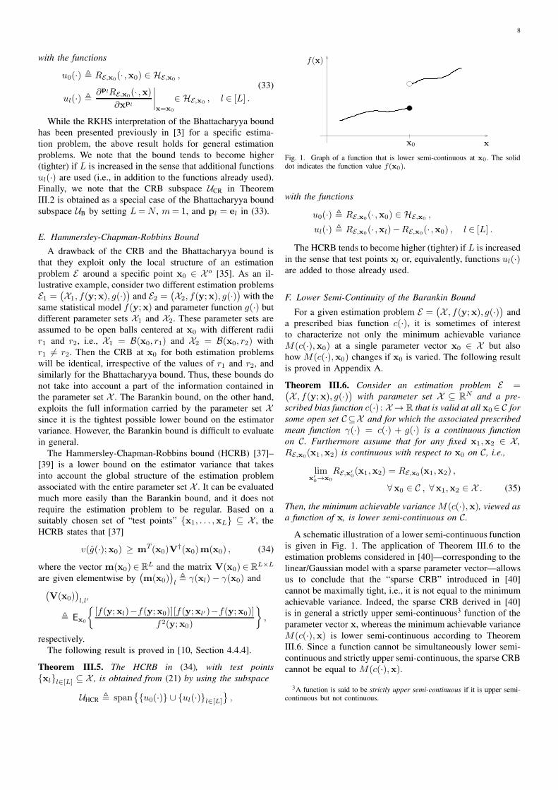
Fig. 1. Graph of a function that is lower semi-continuous at x0. The soliddot indicates the function value f(x0).
with the functions
u0(·) , RE,x0(· ,x0) ∈ HE,x0 ,
ul(·) , RE,x0(· ,xl)−RE,x0(· ,x0) , l ∈ [L] .
The HCRB tends to become higher (tighter) if L is increased
in the sense that test points xl or, equivalently, functions ul(·)are added to those already used.
F. Lower Semi-Continuity of the Barankin Bound
For a given estimation problem E =(
X , f(y;x), g(·))
and
a prescribed bias function c(·), it is sometimes of interest
to characterize not only the minimum achievable variance
M(c(·),x0) at a single parameter vector x0 ∈ X but also
how M(c(·),x0) changes if x0 is varied. The following result
is proved in Appendix A.
Theorem III.6. Consider an estimation problem E =(
X , f(y;x), g(·))
with parameter set X ⊆ RN and a pre-
scribed bias function c(·) : X → R that is valid at all x0∈ C for
some open set C⊆X and for which the associated prescribed
mean function γ(·) = c(·) + g(·) is a continuous function
on C. Furthermore assume that for any fixed x1,x2 ∈ X ,
RE,x0(x1,x2) is continuous with respect to x0 on C, i.e.,
limx′0→x0
RE,x′0(x1,x2) = RE,x0(x1,x2) ,
∀x0 ∈ C , ∀x1,x2 ∈ X . (35)
Then, the minimum achievable variance M(c(·),x), viewed as
a function of x, is lower semi-continuous on C.
A schematic illustration of a lower semi-continuous function
is given in Fig. 1. The application of Theorem III.6 to the
estimation problems considered in [40]—corresponding to the
linear/Gaussian model with a sparse parameter vector—allows
us to conclude that the “sparse CRB” introduced in [40]
cannot be maximally tight, i.e., it is not equal to the minimum
achievable variance. Indeed, the sparse CRB derived in [40]
is in general a strictly upper semi-continuous3 function of the
parameter vector x, whereas the minimum achievable variance
M(c(·),x) is lower semi-continuous according to Theorem
III.6. Since a function cannot be simultaneously lower semi-
continuous and strictly upper semi-continuous, the sparse CRB
cannot be equal to M(c(·),x).
3A function is said to be strictly upper semi-continuous if it is upper semi-continuous but not continuous.
9
IV. SUFFICIENT STATISTICS
For some estimation problems E =(
X , f(y;x), g(·))
, the
observation y ∈ RM contains information that is irrelevant to
E , and thus y can be compressed in some sense. Accordingly,
let us replace y by a transformed observation z = t(y) ∈RK,
with a deterministic mapping t(·) : RM → RK. A compression
is achieved if K<M . Any transformed observation z = t(y)is termed a statistic, and it is said to be a sufficient statistic
if it preserves all the information that is relevant to E [1],
[15]–[18], [41]. In particular, a sufficient statistic preserves the
minimum achievable variance (Barankin bound) M(c(·),x0).In the following, the mapping t(·) will be assumed to be
measurable.
For a given reference parameter vector x0 ∈ X , we
consider estimation problems E =(
X , f(y;x), g(·))
for
which there exists a dominating measure µE such that the
pdfs {f(y;x)}x∈X are well defined with respect to µE and
condition (5) is satisfied. The Neyman-Fisher factorization
theorem [15]–[18] then states that the statistic z = t(y) is
sufficient for E =(
X , f(y;x), g(·))
if and only if f(y;x)can be factored as
f(y;x) = h(t(y);x) k(y) , (36)
where h(· ;x) and k(·) are nonnegative functions and the
function k(·) does not depend on x. Relation (36) has to be
satisfied for every y ∈ RM except for a set of measure zero
with respect to the dominating measure µE .
The probability measure on RK (equipped with the system
of K-dimensional Borel sets, cf. [1, Section 10]) that is
induced by the random vector z = t(y) is obtained as µzx =
µyxt
−1 [16], [17]. According to Section II-B1, under condition
(5), the measure µyx0
dominates the measures {µyx}x∈X . This,
in turn, implies via [16, Lemma 4] that the measure µzx0
dominates the measures {µzx}x∈X , and therefore that, for each
x ∈ X , there exists a pdf f(z;x) with respect to the measure
µzx0
. This pdf is given by the following result. (Note that we
do not assume condition (8).)
Lemma IV.1. Consider an estimation problem E =(
X , f(y;x), g(·))
satisfying (5), i.e., which is such that the
Radon-Nikodym derivative of µyx with respect to µy
x0is well
defined and given by the likelihood ratio ρE,x0(y,x). Further-
more consider a sufficient statistic z = t(y) for E . Then, the
pdf of z with respect to the dominating measure µzx0
is given
by
f(z;x) =h(z;x)
h(z;x0), (37)
where the function h(z;x) is obtained from the factorization
(36).
Proof : The pdf f(z;x) of z with respect to µzx0
is defined
by the relation
Ex0
{
IA(z)f(z;x)}
= Px{z ∈ A} , (38)
which has to be satisfied for every measurable set A ⊆ RK
[1]. Denoting the pre-image of A under the mapping t(·) by
t−1(A) ,{
y∣
∣t(y) ∈ A}
⊆ RM, we have
Ex0
{
IA(z)h(z;x)
h(z;x0)
}
(a)= Ex0
{
IA(t(y))h(t(y);x)
h(t(y);x0)
}
= Ex0
{
It−1(A)(y)h(t(y);x)
h(t(y);x0)
}
(36),(6)= Ex0
{
It−1(A)(y)ρE,x0 (y,x)
}
(b)= Px{y ∈ t−1(A)}
= Px{z ∈A} , (39)
where step (a) follows from [1, Theorem 16.12] and (b) is
due to the fact that the Radon-Nikodym derivative of µyx with
respect to µyx0
is given by ρE,x0(y,x) (cf. (6)), as explained
in Section II-B1. Comparing (39) with (38), we conclude thath(z;x)h(z;x0)
= f(z;x) up to differences on a set of measure zero
(with respect to µzx0
). Note that because we require t(·) to be
a measurable mapping, it is guaranteed that the set t−1(A) ={
y∣
∣t(y) ∈A}
is measurable for any measurable set A ⊆ RK.
�
Consider next an estimation problem E =(
X , f(y;x), g(·))
satisfying (8), so that the kernel RE,x0(· , ·) exists according to
(9). Let z = t(y) be a sufficient statistic. We can then define
the modified estimation problem E ′ ,(
X , f(z;x), g(·))
,
which is based on the observation z and whose statistical
model is given by the pdf f(z;x) (cf. (37)). The following
theorem states that the RKHS associated with E ′ equals the
RKHS associated with E .
Theorem IV.2. Consider an estimation problem E =(
X , f(y;x), g(·))
satisfying (8) and a reference parameter
vector x0∈X . For a sufficient statistic z = t(y), consider the
modified estimation problem E ′ =(
X , f(z;x), g(·))
. Then, E ′
also satisfies (8) and furthermore RE′,x0(· , ·) = RE,x0(· , ·)and HE′,x0 = HE,x0 .
Proof : We have
RE,x0(x1,x2)(9),(7)= Ex0
{
ρE,x0(y,x1)ρE,x0(y,x2)}
(36),(6)= Ex0
{
h(t(y);x1)h(t(y);x2)
h2(t(y);x0)
}
(a)= Ex0
{
h(z;x1)h(z;x2)
h2(z;x0)
}
(37)= Ex0
{
f(z;x1)f(z;x2)}
(37)= Ex0
{
f(z;x1)f(z;x2)
f2(z;x0)
}
(7),(9)= RE′,x0(x1,x2) , (40)
where, as before, step (a) follows from [1, Theorem 16.12].
From (40), we conclude that if E satisfies (8) then so does E ′.
Moreover, from RE′,x0(· , ·) = RE,x0(· , ·) in (40), it follows
that HE′,x0 = H(RE′,x0) equals HE,x0 = H(RE,x0). �
Intuitively, one might expect that the RKHS associated with
a sufficient statistic should be typically “smaller” or “simpler”
than the RKHS associated with the original observation, since
in general the sufficient statistic is a compressed and “more
10
concise” version of the observation. However, Theorem IV.2
states that the RKHS remains unchanged by this compression.
One possible interpretation of this fact is that the RKHS
description of an estimation problem is already “maximally
efficient” in the sense that it cannot be reduced or simplified by
using a compressed (yet sufficiently informative) observation.
V. MVE FOR THE EXPONENTIAL FAMILY
An important class of estimation problems is defined by
statistical models belonging to an exponential family. Such
models are of considerable interest in the context of MVE
because, under mild conditions, the existence of a UMV
estimator is guaranteed. Furthermore, any estimation problem
that admits an efficient estimator, i.e., an estimator whose
variance attains the CRB, must be necessarily based on an
exponential family [15, Theorem 5.12]. In this section, we
will characterize the RKHS for this class and use it to derive
lower variance bounds.
A. Review of the Exponential Family
An exponential family is defined as the following
parametrized set of pdfs {f(y;x)}x∈X (with respect to the
Lebesgue measure on RM ) [15], [42], [43]:
f(y;x) = exp(
φT(y)u(x)−A(x))
h(y) ,
with the sufficient statistic φ(·) : RM → RQ, the parameter
function u(·) : RN → RQ, the cumulant function A(·) : RN →
R, and the weight function h(·) : RM → R. Many well-known
statistical models are special instances of an exponential family
[43]. Without loss of generality, we can restrict ourselves to an
exponential family in canonical form [15], for which Q =Nand u(x) = x, i.e.,
f (A)(y;x) = exp(
φT(y)x−A(x))
h(y) . (41)
Here, the superscript (A) emphasizes the importance of the cu-
mulant function A(·) in the characterization of an exponential
family. In what follows, we assume that the parameter space
is chosen as X ⊆N , where N ⊆ RN is the natural parameter
space defined as
N ,
{
x ∈ RN
∣
∣
∣
∣
∫
RM
exp(
φT(y)x)
h(y) dy < ∞
}
.
From the normalization constraint∫
RM f (A)(y;x)dy = 1, it
follows that the cumulant function A(·) is determined by the
sufficient statistic φ(·) and the weight function h(·) as
A(x) = log
(∫
RM
exp(
φT(y)x)
h(y) dy
)
, x ∈N .
The moment-generating function of f (A)(y;x) is defined as
λ(x) , exp(A(x)) =
∫
RM
exp(
φT(y)x)
h(y) dy , x ∈N .
(42)Note that
N ={
x ∈ RN∣
∣λ(x) < ∞}
.
Assuming a random vector y ∼ f (A)(y;x), it is known [42,
Theorem 2.2], [43, Proposition 3.1] that for any x ∈ X o and
p ∈ ZN+ , the moments Ex
{
φp(y)}
exist, i.e., Ex
{
φp(y)}
<∞, and they can be calculated from the partial derivatives of
λ(x) according to
Ex
{
φp(y)}
=1
λ(x)
∂pλ(x)
∂xp. (43)
Thus, the partial derivatives∂pλ(x)∂xp exist for any x∈X o and
p∈ZN+ . Moreover, they depend continuously on x ∈ X o [42],
[43].
B. RKHS Associated with an Exponential Family Based MVP
Consider an estimation problem E(A) ,(
X , f (A)(y;x),g(·))
with an exponential family statistical model
{f (A)(y;x)}x∈X as defined in (41), and a fixed x0 ∈ X .
Consider further the RKHS HE(A),x0. Its kernel is obtained as
RE(A),x0(x1,x2)
(9)= Ex0
{
f (A)(y;x1)f(A)(y;x2)
(f (A)(y;x0))2
}
(44)
(41)= Ex0
{
exp(
φT(y)x1 −A(x1))
exp(
φT(y)x2 −A(x2))
exp(
2[
φT(y)x0 −A(x0)])
}
= Ex0
{
exp(
φT(y)(x1+x2− 2x0)−A(x1)−A(x2)
+ 2A(x0))}
(41)= exp
(
−A(x1)−A(x2) + 2A(x0))
×
∫
RM
exp(
φT(y)(x1+x2 − 2x0))
× exp(
φT(y)x0 −A(x0))
h(y) dy
= exp(
−A(x1)−A(x2) +A(x0))
×
∫
RM
exp(
φT(y)(x1+x2 −x0))
h(y) dy
(42)=
λ(x1+x2−x0)λ(x0)
λ(x1)λ(x2). (45)
Because (44) and (45) are equal, we see that condition
(8) is satisfied, i.e., Ex0
{
f(A)(y;x1)f(A)(y;x2)
(f(A)(y;x0))2
}
< ∞ for all
x1,x2 ∈ X , if and only ifλ(x1+x2−x0) λ(x0)
λ(x1)λ(x2)< ∞ for all
x1,x2 ∈ X . Since x0 ∈ X ⊆ N , we have λ(x0) < ∞.
Furthermore, λ(x) 6= 0 for all x ∈ X . Therefore, (8) is satisfied
if and only if λ(x1 + x2 − x0) < ∞. We conclude that for
an estimation problem whose statistical model belongs to an
exponential family, condition (8) is equivalent to
x1,x2 ∈ X ⇒ x1+x2 −x0 ∈ N . (46)
Furthermore, from (45) and the fact that the partial derivatives∂pλ(x)∂xp exist for any x ∈ X o and p ∈ Z
N+ and depend
continuously on x ∈ X o, we can conclude that the RKHS
HE(A),x0is differentiable up to any order. We summarize this
finding in the following lemma.
Lemma V.1. Consider an estimation problem E(A) =(
X ,f (A)(y;x), g(·)
)
associated with an exponential family (cf.
(41)) with natural parameter space N . We assume that X ⊆ Nand that X satisfies condition (46) for some reference param-
eter vector x0 ∈ X . Then, the kernel RE(A),x0(x1,x2) and the
RKHS HE(A),x0are differentiable up to any order m.
11
Next, by combining Lemma V.1 with (20), we will derive
simple lower bounds on the variance of estimators with a
prescribed bias function.
C. Variance Bounds for the Exponential Family
If X o is nonempty, the sufficient statistic φ(·) is a complete
sufficient statistic for the estimation problem E(A), and thus
there exists a UMV estimator gUMV(·) for any valid bias
function c(·) [15, p. 42]. This UMV estimator is given by
the conditional expectation4
gUMV(y) = Ex{g0(y)|φ(y)} , (47)
where g0(·) is any estimator with bias function c(·), i.e.,
b(g0(·);x0) = c(x) for all x ∈ X . The minimum achievable
variance M(c(·),x0) is then equal to the variance of gUMV(·)at x0, i.e., M(c(·),x0) = v(gUMV(·);x0) [15, p. 89]. However,
it may be difficult to actually construct the UMV estimator via
(47) and to calculate its variance. In fact, it may be already a
difficult task to find an estimator g0(·) whose bias function
equals c(·). Therefore, it is still of interest to find simple
closed-form lower bounds on the variance of any estimator
with bias c(·).
Theorem V.2. Consider an estimation problem E(A) =(
X ,f (A)(y;x), g(·)
)
with parameter set X ⊆ N satisfying (46)
and a finite set of multi-indices {pl}l∈[L] ⊆ ZN+ . Then, at any
x0∈X o, the variance of any estimator g(·) with mean function
γ(x) = Ex{g(y)} and finite variance at x0 is lower bounded
as
v(g(·);x0) ≥ nT(x0)S†(x0)n(x0) − γ2(x0) , (48)
where the vector n(x0) ∈ RL and the matrix S(x0) ∈ R
L×L
are given elementwise by
(
n(x0))
l,∑
p≤pl
(
pl
p
)
Ex0
{
φpl−p(y)} ∂pγ(x)
∂xp
∣
∣
∣
∣
x=x0
(49)
(
S(x0))
l,l′, Ex0
{
φpl+pl′ (y)}
, (50)
respectively. Here,∑
p≤pldenotes the sum over all multi-
indices p ∈ ZN+ such that pk ≤ (pl)k for k ∈ [N ], and
(
pl
p
)
,∏N
k=1
(
(pl)kpk
)
.
A proof of this result is provided in Appendix B. This proof
shows that the bound (48) is obtained by projecting an appro-
priately transformed version of the mean function γ(·) onto the
finite-dimensional subspace U = span{
r(pl)x0 (·)
}
l∈[L]of an
appropriately defined RKHS H(R), with the functions r(pl)x0 (·)
given by (19). If we increase the set{
r(pl)x0 (·)
}
l∈[L]by adding
further functions r(p′)x0 (·) with multi-indices p′ /∈ {pl}l∈[L],
the subspace tends to become higher-dimensional and in turn
the lower bound (48) becomes higher, i.e., tighter.
The requirement of a finite variance v(g(·);x0) in Theorem
V.2 implies via (10) that γ(·) ∈ HE(A),x0. This, in turn, guaran-
tees via (20)—which can be invoked since due to Lemma V.1
4The conditional expectation in (47) can be taken with respect to themeasure µy
x for an arbitrary x ∈ X . Indeed, since φ(·) is a sufficient statistic,Ex{g0(y)|φ(y)} yields the same result for every x ∈ X .
the RKHS HE(A),x0is differentiable up to any order at x0—the
existence of the partial derivatives∂pγ(x)∂xp
∣
∣
x=x0. Note also that
the bound (48) depends on the mean function γ(·) only via
the local behavior of γ(·) as given by the partial derivatives
of γ(·) at x0 up to a suitable order.
Evaluating the bound (48) requires computation of the
moments Ex0
{
φp(y)}
. This can be done by means of message
passing algorithms [43].
For the choice L = N and pl = el, the bound (48) is closely
related to the CRB obtained for the estimation problem E(A).
In fact, the CRB for E(A) is obtained as [15, Theorem 2.6.2]
v(g(·);x0) ≥ nT(x0)J†(x0)n(x0) , (51)
with(
n(x0))
l= ∂γ(x)
∂xl
∣
∣
x=x0and the Fisher information matrix
given by
J(x0) = Ex0
{(
φ(y)−Ex0{φ(y)})(
φ(y) − Ex0{φ(y)})T}
,
i.e., the covariance matrix of the sufficient statistic vector
φ(y). On the other hand, evaluating the bound (48) for L = Nand pl = el and assuming without loss of generality5 that
γ(x0) = 0, we obtain
v(g(·);x0) ≥ nT(x0)S†(x0)n(x0) , (52)
with n(x0) as before and
S(x0) = Ex0
{
φ(y)φT (y)}
.
Thus, the only difference is that the CRB in (51) involves the
covariance matrix of the sufficient statistic φ(y) whereas the
bound in (52) involves the correlation matrix of φ(y).
D. Reducing the Parameter Set
Using the RKHS framework, we will now show that,
under mild conditions, the minimum achievable variance
M(c(·),x0) for an exponential family type estimation prob-
lem E(A) =(
X , f (A)(y;x), g(·))
is invariant to reductions
of the parameter set X . Consider two estimation problems
E =(
X , f(y;x), g(·))
and E ′ =(
X ′, f(y;x), g(·)∣
∣
X ′
)
—for
now, not necessarily of the exponential family type—that differ
only in their parameter sets X and X ′. More specifically,
E ′ is obtained from E by reducing the parameter set, i.e.,
X ′ ⊆ X . For these two estimation problems, we consider
corresponding MVPs at a specific parameter vector x0 ∈ X ′
and for a certain prescribed bias function c(·). More precisely,
c(·) is the prescribed bias function for E on the set X , while
the prescribed bias function for E ′ is the restriction of c(·) to
X ′, c(·)∣
∣
X ′. We will denote the minimum achievable variances
of the MVPs corresponding to E and E ′ by M(c(·),x0)and M ′
(
c(·)∣
∣
X ′,x0
)
, respectively. From (23), it follows that
M ′(
c(·)∣
∣
X ′,x0
)
≤ M(c(·),x0), since taking the supremum
over a reduced set can never result in an increase of the
supremum.
The effect that a reduction of the parameter set X has on the
minimum achievable variance can be analyzed conveniently
5Indeed, as we observed after Lemma III.1, the minimum achievablevariance at x0 for prescribed mean function γ(·) is equal to the minimumachievable variance at x0 for prescribed mean function γ(x) = γ(x)−γ(x0).Note that γ(x0) = 0.
12
within the RKHS framework. This is based on the following
result [21]: Consider an RKHS H(R1) of functions f(·) :D1 → R, with kernel R1(· , ·) : D1×D1 → R. Let D2 ⊆ D1.
Then, the set of functions{
f(·) , f(·)∣
∣
D2
∣
∣ f(·) ∈ H(R1)}
that is obtained by restricting each function f(·) ∈ H(R1) to
the subdomain D2 coincides with the RKHS H(R2) whose
kernel R2(· , ·) : D2 ×D2 → R is the restriction of R1(· , ·) :D1×D1→R to the subdomain D2 ×D2, i.e.,
H(R2) ={
f(·) , f(·)∣
∣
D2
∣
∣ f(·) ∈ H(R1)}
,
with R2(· , ·) , R1(· , ·)∣
∣
D2×D2. (53)
Furthermore, the norm of an element f(·) ∈ H(R2) is equal
to the minimum of the norms of all functions f(·) ∈ H(R1)that coincide with f(·) on D2, i.e.,
‖f(·)‖H(R2)= min
f(·)∈H(R1)
f(·)∣
∣
D2= f(·)
‖f(·)‖H(R1). (54)
Consider an arbitrary but fixed f(·) ∈ H(R1), and let
f(·) , f(·)∣
∣
D2. Because f(·) ∈ H(R2), we can calcu-
late ‖f(·)‖H(R2). From (54), we obtain for ‖f(·)‖H(R2)
=∥
∥f(·)∣
∣
D2
∥
∥
H(R2)the inequality
∥
∥f(·)∣
∣
D2
∥
∥
H(R2)≤ ‖f(·)‖H(R1)
, (55)
which holds for all f(·) ∈H(R1).Let us now return to the MVPs corresponding to E and E ′.
From (55) with D1 = X , D2 = X ′, H(R1) = HE,x0 , and
H(R2) = HE′,x0 , we can conclude that, for any x0 ∈ X ′,
M ′(
c(·)∣
∣
X ′,x0
) (11)=∥
∥γ(·)∣
∣
X ′
∥
∥
2
HE′,x0
− γ2(x0)
(55)
≤ ‖γ(·)‖2HE,x0− γ2(x0)
= M(c(·),x0) . (56)
Here, we also used the fact that γ(·)∣
∣
X ′= c(·)
∣
∣
X ′+ g(·)
∣
∣
X ′.
The inequality in (56) means that a reduction of the pa-
rameter set X can never result in a deterioration of the
achievable performance, i.e., in a higher minimum achievable
variance. Besides this rather intuitive fact, the result (53) has
the following consequence: Consider an estimation problem
E =(
X , f(y;x), g(·))
whose statistical model {f(y;x)}x∈X
satisfies (8) at some x0 ∈ X and moreover is contained in
a “larger” model {f(y;x)}x∈X with X ⊇ X . If the larger
model {f(y;x)}x∈X also satisfies (8), it follows from (53)
that a prescribed bias function c(·) : X → R can only
be valid for E at x0 if it is the restriction of a function
c′(·) : X → R that is a valid bias function for the estimation
problem E =(
X, f(y;x), g(·))
at x0. This holds true since
every valid bias function for E at x0 corresponds to a mean
function that is an element of the RKHS HE,x0 , which by
(53) consists precisely of the restrictions of the elements of
the RKHS HE,x0, which by (10) consists precisely of the mean
functions corresponding to bias functions that are valid for Eat x0.
For the remainder of this section, we restrict our discussion
to estimation problems E(A) =(
X , f (A)(y;x), g(·))
whose
statistical model is an exponential family model. The next re-
sult characterizes the analytic properties of the mean functions
γ(·) that belong to an RKHS HE(A),x0. A proof is provided in
Appendix C.
Lemma V.3. Consider an estimation problem E(A) =(
X , f (A)(y;x), g(·))
with an open parameter set X ⊆ Nsatisfying (46) for some x0 ∈ X . Let γ(·) ∈ HE(A),x0
be
such that the partial derivatives∂pγ(x)∂xp
∣
∣
x=x0vanish for every
multi-index p ∈ ZN+ . Then γ(x) = 0 for all x ∈ X .
Note that since HE(A),x0is differentiable at x0 up
to any order (see Lemma V.1), it contains the function
set{
r(p)x0 (x)
}
p∈ZN+
defined in (19). Moreover, by (20),
for any f(·) ∈ HE(A),x0and any p ∈ Z
N+ , there is
⟨
r(p)x0 (·), f(·)
⟩
HE(A),x0
= ∂pf(x)∂xp
∣
∣
x=x0. Hence, under the as-
sumptions of Lemma V.3, we have that if a function f(·) ∈
HE(A),x0satisfies
⟨
r(p)x0 (·), f(·)
⟩
HE(A),x0
= 0 for all p ∈ ZN+ ,
then f(·) ≡ 0. Thus, in this case, the set{
r(p)x0 (x)
}
p∈ZN+
is
complete for the RKHS HE(A),x0.
Upon combining (53) and (54) with Lemma V.3, we arrive
at the second main result of this section:
Theorem V.4. Consider an estimation problem E(A) =(
X , f (A)(y;x), g(·))
with an open parameter set X ⊆ Nsatisfying (46) for some x0∈X , and a prescribed bias function
c(·) that is valid for E(A) at x0. Furthermore consider a
reduced parameter set X1 ⊆ X such that x0 ∈ X o1 . Let
E(A)1 ,
(
X1, f(A)(y;x), g(·)
)
denote the estimation problem
that is obtained from E(A) by reducing the parameter set to
X1, and let c1(·) , c(·)∣
∣
X1. Then, the minimum achievable
variance for the restricted estimation problem E(A)1 and the
restricted bias function c1(·), denoted by M1(c1(·),x0), is
equal to the minimum achievable variance for the original
estimation problem E(A) and the original bias function c(·),i.e.,
M1(c1(·),x0) = M(c(·),x0) .
A proof of this theorem is provided in Appendix D. Note
that the requirement x0 ∈ X o1 of the theorem implies that
the reduced parameter set X1 must contain a neighborhood
of x0, i.e., an open ball B(x0, r) with some radius r > 0.
The message of the theorem is that, for an estimation problem
based on an exponential family, parameter set reductions have
no effect on the minimum achievable variance at x0 as long
as the reduced parameter set contains a neighborhood of x0.
VI. CONCLUSION
The mathematical framework of reproducing kernel Hilbert
spaces (RKHS) provides powerful tools for the analysis of
minimum variance estimation (MVE) problems. Building upon
the theoretical foundation developed in the seminal papers
[2] and [3], we derived novel results concerning the RKHS-
based analysis of lower variance bounds for MVE, of sufficient
statistics, and of MVE problems conforming to an exponential
family of distributions. More specifically, we presented an
RKHS-based geometric interpretation of several well-known
13
lower bounds on the estimator variance. We showed that
each of these bounds is related to the orthogonal projection
onto an associated subspace of the RKHS. In particular, the
subspace associated with the Cramér–Rao bound is based
on the strong structural properties of a differentiable RKHS.
For a wide class of estimation problems, we proved that the
minimum achievable variance, which is the tightest possible
lower bound on the estimator variance (Barankin bound), is
a lower semi-continuous function of the parameter vector.
In some cases, this fact can be used to show that a given
lower bound on the estimator variance is not maximally tight.
Furthermore, we proved that the RKHS associated with an
estimation problem remains unchanged if the observation is
replaced by a sufficient statistic.
Finally, we specialized the RKHS description to estimation
problems whose observation conforms to an exponential fam-
ily of distributions. We showed that the kernel of the RKHS
has a particularly simple expression in terms of the moment-
generating function of the exponential family, and that the
RKHS itself is differentiable up to any order. Using this
differentiability, we derived novel closed-form lower bounds
on the estimator variance. We also showed that a reduction of
the parameter set has no effect on the minimum achievable
variance at a given reference parameter vector x0 if the
reduced parameter set contains a neighborhood of x0.
Promising directions for future work include the practical
implementation of message passing algorithms for the efficient
computation of the lower variance bounds for exponential
families derived in Section V-C. Furthermore, in view of the
close relations between exponential families and probabilistic
graphical models [43], it would be interesting to explore the
relations between the graph-theoretic properties of the graph
associated with an exponential family and the properties of
the RKHS associated with that exponential family.
APPENDIX A
PROOF OF THEOREM III.6
We first note that our assumption that the prescribed bias
function c(·) is valid for E at every x ∈ C has two con-
sequences. First, M(c(·),x) < ∞ for every x ∈ C (cf.
our definition of the validity of a bias function in Section
II-A); second, due to (10), the prescribed mean function
γ(·) = c(·) + g(·) belongs to HE,x for every x ∈ C.
Following [2], we define the linear span of a kernel function
R(· , ·) : X ×X → R, denoted by L(R), as the set of all
functions f(·) : X → R that are finite linear combinations of
the form
f(·) =∑
l∈[L]
alR(·,xl) , with xl ∈ X , al ∈ R , L ∈ N . (57)
The linear span L(R) can be used to express the norm of any
function h(·) ∈H(R) according to
‖h(·)‖2H(R) = supf(·)∈L(R)
‖f(·)‖2H(R)>0
〈h(·), f(·)〉2H(R)
‖f(·)‖2H(R)
. (58)
This expression can be shown by combining [10, Theorem
3.1.2] and [10, Theorem 3.2.2]. We can now develop the
minimum achievable variance M(c(·),x) as follows:
M(c(·),x)(11)= ‖γ(·)‖2HE,x
− γ2(x)
(58)= sup
f(·)∈L(RE,x)
‖f(·)‖2HE,x
>0
〈γ(·), f(·)〉2HE,x
‖f(·)‖2HE,x
− γ2(x) .
Using (57) and letting D , {x1, . . . ,xL}, a , (a1 · · · aL)T,
and AD ,{
a ∈ RL∣
∣
∑
l,l′∈[L] alal′RE,x(xl,xl′) > 0}
, we
obtain further
M(c(·),x) = supD⊆X ,L∈N,a∈AD
hD,a(x) . (59)
Here, our notation supD⊆X ,L∈N,a∈ADindicates that the
supremum is taken not only with respect to the elements xl of
D but also with respect to the size of D, L= |D|; furthermore,
the function hD,a(·) : X → R is given by
hD,a(x) ,
⟨
γ(·),∑
l∈[L] alRE,x(·,xl)⟩2
HE,x
∥
∥
∑
l∈[L] alRE,x(·,xl)∥
∥
2
HE,x
− γ2(x)
=
(∑
l∈[L] al⟨
γ(·), RE,x(·,xl)⟩
HE,x
)2
∑
l,l′∈[L] alal′⟨
RE,x(·,xl)RE,x(·,xl′)⟩
HE,x
− γ2(x)
(4)=
(∑
l∈[L] alγ(xl))2
∑
l,l′∈[L] alal′RE,x(xl,xl′ )− γ2(x) .
For any finite set D = {x1, . . . ,xL} ⊆ X and any a ∈ AD , it
follows from our assumptions of continuity of RE,x(· , ·) with
respect to x on C (see (35)) and continuity of γ(x) on C that
the function hD,a(x) is continuous in a neighborhood around
any point x0 ∈ C. Thus, for any x0 ∈ C, there exists a radius
δ0 > 0 such that hD,a(x) is continuous on B(x0, δ0) ⊆ C.
We will now show that the function M(c(·),x) given by
(59) is lower semi-continuous at every x0 ∈ C, i.e., for any
x0 ∈ C and ε > 0, we can find a radius r > 0 such that
M(c(·),x) ≥ M(c(·),x0)−ε , for all x ∈ B(x0, r) . (60)
Due to (59), there must be a finite subset D0 ⊆X and a vector
a0 ∈ AD0 such that6
hD0,a0(x0) ≥ M(c(·),x0)−ε
2, (61)
for any given ε > 0. Furthermore, since hD0,a0(x) is contin-
uous on B(x0, δ0) as shown above, there is a radius r0 > 0(with r0 ≤ δ0) such that
hD0,a0(x) ≥ hD0,a0(x0)−ε
2, for all x ∈ B(x0, r0) . (62)
6Indeed, if (61) were not true, we would have hD,a(x0) < M(c(·),x0)−ε/2 for every choice of D and a. This, in turn, would imply that
supD⊆X ,L∈N,a∈AD
hD,a(x0) ≤ M(c(·),x0)−ε
2< M(c(·),x0) ,
yielding the contradiction
M(c(·),x0)(59)= sup
D⊆X ,L∈N,a∈AD
hD,a(x0) < M(c(·),x0) .
14
By combining this inequality with (61), it follows that there
is a radius r > 0 (with r ≤ δ0) such that for any x ∈ B(x0, r)we have
hD0,a0(x)(62)
≥ hD0,a0(x0)−ε
2
(61)
≥ M(c(·),x0)− ε , (63)
and further
M(c(·),x)(59)= sup
D⊆X ,L∈N,a∈AD
hD,a(x)
≥ hD0,a0(x)
(63)
≥ M(c(·),x0)− ε .
Thus, for any given ε > 0, there is a radius r > 0 (with r ≤ δ0)
such that M(c(·),x) ≥ M(c(·),x0) − ε for all x∈B(x0, r),i.e., (60) has been proved.
APPENDIX B
PROOF OF THEOREM V.2
The bound (48) in Theorem V.2 is derived by using an
isometry between the RKHS HE(A),x0and the RKHS H(R)
that is defined by the kernel
R(· , ·) : X×X → R , R(x1,x2) =λ(x1+x2 −x0)
λ(x0). (64)
It is easily verified that R(· , ·) and, thus, H(R) are differen-
tiable up to any order. Invoking [10, Theorem 3.3.4], it can be
shown that the two RKHSs HE(A),x0and H(R) are isometric
and a specific congruence J : HE(A),x0→ H(R) is given by
J[f(·)] =λ(x)
λ(x0)f(x) , f(·) ∈ HE(A),x0
. (65)
Similarly to the bound (21), we can then obtain a lower bound
on v(g(·);x0) via an orthogonal projection onto a subspace
of H(R). Indeed, with c(·) = γ(·) − g(·) denoting the bias
function of the estimator g(·), we have
v(g(·);x0)(3)
≥ M(c(·),x0)
(11)= ‖γ(·)‖2H
E(A),x0
− γ2(x0)
(a)=∥
∥J[γ(·)]∥
∥
2
H(R)− γ2(x0)
≥∥
∥
(
J[γ(·)])
U
∥
∥
2
H(R)− γ2(x0) , (66)
for an arbitrary subspace U ⊆H(R). Here, step (a) is due to
the fact that J is a congruence, and (·)U denotes orthogonal
projection onto U . The bound (48) is obtained from (66) by
choosing the subspace as U , span{
r(pl)x0 (·)
}
l∈[L], with the
functions r(pl)x0 (·) ∈ H(R) as defined in (19), i.e., r
(pl)x0 (x) =
∂plR(x,x2)
∂xpl2
∣
∣
x2=x0.
Let us denote the image of γ(·) under the isometry J by
γ(·) , J[γ(·)]. According to (65),
γ(x) =λ(x)
λ(x0)γ(x) . (67)
Furthermore, the variance bound (66) reads
v(g(·);x0) ≥ ‖γU(·)‖2H(R) − γ2(x0) .
Using (15), we obtain further
v(g(·);x0) ≥ nT(x0)S†(x0)n(x0) − γ2(x0) , (68)
where, according to (16), the entries of n(x0) and S(x0) are
calculated as follows:
(
n(x0))
l
(16)=⟨
γ(·), r(pl)x0
(·)⟩
H(R)
(20)=
∂pl γ(x)
∂xpl
∣
∣
∣
∣
x=x0
(67)=
1
λ(x0)
∂pl [λ(x)γ(x)]
∂xpl
∣
∣
∣
∣
x=x0
(a)=
1
λ(x0)
∑
p≤pl
(
pl
p
)
∂pl−pλ(x)
∂xpl−p
∂pγ(x)
∂xp
∣
∣
∣
∣
x=x0
(43)=∑
p≤pl
(
pl
p
)
Ex0
{
φpl−p(y)} ∂pγ(x)
∂xp
∣
∣
∣
∣
x=x0
(69)
(here, (a) is due to the generalized Leibniz rule for differen-
tiation of a product of two functions [13, p. 104]), and
(
S(x0))
l,l′(16)=⟨
r(pl)x0
(·), r(pl′ )x0
(·)⟩
H(R)
(20)=
∂plr(pl′ )x0 (x)
∂xpl
∣
∣
∣
∣
x=x0
(19)=
∂pl
∂xpl
{
∂pl′R(x,x2)
∂xpl′
2
∣
∣
∣
∣
x2=x0
}∣
∣
∣
∣
x=x0
(64)=
1
λ(x0)
∂pl+pl′λ(x)
∂xpl+pl′
∣
∣
∣
∣
x=x0
(43)= Ex0
{
φpl+pl′ (y)}
. (70)
Note that the application of (20) was based on the differen-
tiability of H(R). Comparing (68), (69), and (70) with (48),
(49), and (50), respectively, we conclude that the theorem is
proved.
APPENDIX C
PROOF OF LEMMA V.3
For E(A) =(
X , f (A)(y;x), g(·))
and x0 ∈ X , we consider
a function γ(·) : X → R belonging to the RKHS HE(A),x0.
The idea of the proof is to reduce the characterization of
γ(·) to that of the LMV estimator g(x0)(·) for prescribed
mean function γ(·). This estimator is guaranteed to exist since
γ(·) ∈ HE(A),x0, and it is given by g(x0)(·) = J[γ(·)] (see
(12)). Trivially, v(
g(x0)(·);x0
)
= M(c(·),x0) < ∞ and
Ex
{
g(x0)(y)} = γ(x) for all x ∈ X . For later use, we also
note that
Ex0
{(
g(x0)(y))2}
= v(
g(x0)(y);x0
)
+(
Ex0
{
g(x0)(y)})2
= M(c(·),x0) + γ2(x0)
< ∞ . (71)
For any exponential family based estimation problem
E(A) =(
X , f (A)(y;x), g(·))
, it follows from [42, Theorem
2.7] that the mean function Ex{g(·)} of any estimator g(·)
15
is analytic7 on the interior T o of the set T ,{
x ∈N∣
∣Ex{|g(y)|} <∞}
. Furthermore, T can be shown to be a
convex set [42, Corollary 2.6]. In particular, the mean function
γ(x) of the LMV estimator g(x0)(·) is analytic on the interior
T o0 of the convex set T0 ,
{
x ∈ N∣
∣Ex{|g(x0)(y)|} <∞}
. However, here we are interested in the behavior of
Ex
{
g(x0)(y)} = γ(x) on the domain X . Therefore, we will
next verify that X ⊆T0.
Using the Hilbert space Hx0 ,{
t(y)∣
∣Ex0{t2(y)} <
∞}
and associated inner product 〈t1(y), t2(y)〉RV =Ex0{t1(y)t2(y)}, we obtain for an arbitrary x ∈ X ⊆N
Ex
{∣
∣g(x0)(y)∣
∣
}
= Ex0
{
∣
∣g(x0)(y)∣
∣
f (A)(y;x)
f (A)(y;x0)
}
=⟨∣
∣g(x0)(y)∣
∣, ρE(A),x0(y,x)
⟩
RV
(a)
≤√
⟨∣
∣g(x0)(y)∣
∣,∣
∣g(x0)(y)∣
∣
⟩
RV
⟨
ρE(A),x0(y,x), ρE(A),x0
(y,x)⟩
RV
=
√
Ex0
{(
g(x0)(y))2} ⟨
ρE(A),x0(y,x), ρE(A),x0
(y,x)⟩
RV
(71),(8)< ∞ ,
where (a) follows from the Cauchy-Schwarz inequality
in the Hilbert space Hx0 . Thus, we have verified that
Ex
{∣
∣g(x0)(y)∣
∣
}
< ∞ on X , which implies that X ⊆ T0.
Moreover, we have
X ⊆ T o0 . (72)
This is implied8 by X ⊆ T0 together with the fact that (by
assumption) X is an open set.
Next, we will show that because of the analyticity of γ(·)on T o
0 , the fact that all partial derivatives of γ(·) vanish at x0
implies that γ(x)=0 for all x∈T o0 , and, in turn, by (72) that
γ(x)=0 for all x∈X . Let us consider the restrictions
γRx1(a) , γ
(
ax1 + (1−a)x0
)
, a∈(−ε, 1 + ε) , (73)
of γ(·) on line segments Rx1 ,{
ax1 + (1− a)x0
∣
∣a ∈(−ε, 1 + ε)
}
, where x1 ∈ T o0 and ε > 0. Here, ε is chosen
sufficiently small such that the vectors xa , x0 − ε(x1 − x0)and xb , x1 + ε(x1 − x0) belong to T o
0 , i.e., xa,xb ∈ T o0 .
Such an ε can always be found, since x0 ∈ T o0 (due to (72))
and x1 ∈ T o0 (by assumption). As can be verified easily, any
vector in Rx1 is a convex combination of the vectors xa and
xb, which both belong to T o0 . Therefore we have Rx1⊆T o
0 for
any x1 ∈T o0 , as the interior T o
0 of the convex set T0 is itself
7Following [14, Definition 2.2.1], we call a function f(·) : U → R definedon some open domain U ⊆ RN analytic if for every point xc ∈ U thereexists a power series
∑p∈ZN
+ap(x−xc)p converging to f(x) for every x
in some neighborhood of xc. Note that the coefficients ap may depend onxc.
8Indeed, assume that the open set X ⊆ T0 contains a vector x′ ∈ X that
does not belong to the interior T o0
. It follows that no single neighborhoodof x
′ can be contained in T0 and, thus, no single neighborhood of x′ can
be contained in X , since X ⊆ T0. However, because x′ belongs to the open
set X =X o, there must be at least one neighborhood of x′ that is contained
in X . Thus, we arrived at a contradiction, which implies that every vectorx′∈ X must belong to T o
0, or, equivalently, that X ⊆ T o
0.
a convex set [44, Theorem 6.2],9 i.e., the interior T o0 contains
any convex combination of its elements.
The function γRx1(·) : (−ε, 1+ε)→ R in (73) is the compo-
sition of the mean function γ(·) : X → R, which is analytic on
T o0 , with the vector-valued function b(·) : (−ε, 1 + ε) → T o
0
given by b(a) = ax1 + (1 − a)x0. Since each component
bl(·) of the function b(·), whose domain is the open interval
(−ε, 1 + ε), is an analytic function, the function γRx1(·) is
itself analytic [14, Proposition 2.2.8].
Since the partial derivatives of γ(·) at x0,∂pγ(x)∂xp
∣
∣
x=x0, are
assumed to vanish for every p ∈ ZN+ , the (ordinary) derivatives
of arbitrary order of the scalar function γRx1(a) vanish at a =
0 (cf. [13, Theorem 9.15]). According to [14, Corollary 1.2.5],
since γRx1(a) is an analytic function, this implies that γRx1
(a)vanishes everywhere on its open domain (−ε, 1 + ε). This, in
turn, implies that γ(·) vanishes on every line segment Rx1
with arbitrary x1∈T o0 and, thus, γ(·) vanishes everywhere on
T o0 . By (72), we finally conclude that γ(·) vanishes everywhere
on X .
APPENDIX D
PROOF OF THEOREM V.4
Because c(·) was assumed valid at x0, the corresponding
mean function γ(·) = c(·) + g(·) is an element of HE(A),x0
(see (10)). Let γ1(·) , γ(·)∣
∣
X1, and note that γ1(·) is the
mean function corresponding to the restricted bias function
c1(·), i.e., γ1(·) = c1(·) + g(·)∣
∣
X1. We have γ1(·) ∈ H
E(A)1 ,x0
due to (10), because γ1(x) is the mean function (evaluated for
x ∈ X1) of an estimator g(·) that has finite variance at x0 ∈ X o1
and whose bias function on X equals c(x). (The existence of
such an estimator g(·) is guaranteed since c(·) was assumed
valid at x0.) For the minimum achievable variance for the
restricted estimation problem, we obtain
M1(c1(·),x0)(11)= ‖γ1(·)‖
2H
E(A)1
,x0
− γ21(x0)
(54)= min
γ′(·)∈HE(A),x0
γ′(·)∣
∣
X1=γ1(·)
‖γ′(·)‖2H
E(A),x0
− γ21(x0) . (74)
However, the only function γ′(·) ∈ HE(A),x0that satisfies
γ′(·)∣
∣
X1= γ1(·) is the mean function γ(·). This is a conse-
quence of Lemma V.3 and can be verified as follows. Consider
a function γ′(·) ∈ HE(A),x0that satisfies γ′(·)
∣
∣
X1= γ1(·).
By the definition of γ1(·), we also have γ(·)∣
∣
X1= γ1(·).
Therefore, the difference γ′′(·) , γ′(·) − γ(·) ∈ HE(A),x0
satisfies γ′′(·)∣
∣
X1= γ′(·)
∣
∣
X1− γ(·)
∣
∣
X1= γ1(·) − γ1(·) = 0,
i.e., γ′′(x) = 0 for all x ∈ X1. Since x0 ∈ X o1 , this implies
that∂pγ′′(x)
∂xp
∣
∣
x=x0= 0 for all p ∈ Z
N+ . It then follows
from Lemma V.3 that γ′′(x) = 0 for all x ∈ X and, thus,
γ′(x) = γ(x) for all x ∈ X . This shows that γ(·) is the unique
9Strictly speaking, [44, Theorem 6.2] states that the relative interior of aconvex set is a convex set. However, since we assume that X is open withnonempty interior and therefore, by (72), also T0 has a nonempty interior, therelative interior of T0 coincides with the interior of T0.
16
function satisfying γ(·)∣
∣
X1= γ1(·). Therefore, we have
minγ′(·)∈H
E(A),x0
γ′(·)∣
∣
X1=γ1(·)
‖γ′(·)‖2H
E(A),x0
= ‖γ(·)‖2HE(A),x0
,
and thus (74) becomes
M1(c1(·),x0) = ‖γ(·)‖2HE(A),x0
− γ21(x0)
= ‖γ(·)‖2HE(A),x0
− γ2(x0)
(11)= M(c(·),x0) .
Here, the second equality is due to the fact that γ1(x0) =γ(x0) (because x0 ∈ X o
1 ).
REFERENCES
[1] P. Billingsley, Probability and Measure, 3rd ed. New York: Wiley,1995.
[2] E. Parzen, “Statistical inference on time series by Hilbert space methods,I.” Appl. Math. Stat. Lab., Stanford University, Stanford, CA, Tech.Rep. 23, Jan. 1959.
[3] D. D. Duttweiler and T. Kailath, “RKHS approach to detection andestimation problems – Part V: Parameter estimation,” IEEE Trans. Inf.Theory, vol. 19, no. 1, pp. 29–37, Jan. 1973.
[4] S. Smale and D.-X. Zhou, “Learning theory estimates via integraloperators and their approximations,” Constr. Approx., vol. 26, pp. 153–172, 2007.
[5] F. Cucker and S. Smale, “On the mathematical foundations of learning,”Bull. Amer. Math. Soc., vol. 39, pp. 1–49, 2002.
[6] S. Schmutzhard, A. Jung, F. Hlawatsch, Z. Ben-Haim, and Y. C. Eldar,“A lower bound on the estimator variance for the sparse linear model,” inProc. 44th Asilomar Conf. Signals, Systems, Computers, Pacific Grove,CA, Nov. 2010, pp. 1976–1980.
[7] S. Schmutzhard, A. Jung, and F. Hlawatsch, “Minimum variance esti-mation for the sparse signal in noise model,” in Proc. IEEE ISIT 2011,St. Petersburg, Russia, Jul.–Aug. 2011, pp. 124–128.
[8] A. Jung, S. Schmutzhard, F. Hlawatsch, and A. O. Hero III, “Perfor-mance bounds for sparse parametric covariance estimation in Gaussianmodels,” in Proc. IEEE ICASSP 2011, Prague, Czech Republic, May2011, pp. 4156–4159.
[9] T. Kailath, “RKHS approach to detection and estimation problems – PartI: Deterministic signals in Gaussian noise,” IEEE Trans. Inf. Theory,vol. 17, no. 5, pp. 530–549, Sep. 1971.
[10] A. Jung, “An RKHS Approach to Estimation with Sparsity Constraints,”Ph.D. dissertation, Vienna University of Technology, 2011, availableonline: arXiv:1311.5768.
[11] G. H. Golub and C. F. Van Loan, Matrix Computations, 3rd ed.Baltimore, MD: Johns Hopkins University Press, 1996.
[12] B. R. Gelbaum and J. M. Olmsted, Counterexamples in Analysis.Mineola, NY: Dover Publications, 2003.
[13] W. Rudin, Principles of Mathematical Analysis, 3rd ed. New York:McGraw-Hill, 1976.
[14] S. G. Krantz and H. R. Parks, A Primer of Real Analytic Functions,2nd ed. Boston, MA: Birkhäuser, 2002.
[15] E. L. Lehmann and G. Casella, Theory of Point Estimation, 2nd ed.New York: Springer, 1998.
[16] P. R. Halmos and L. J. Savage, “Application of the Radon-Nikodymtheorem to the theory of sufficient statistics,” Ann. Math. Statist., vol. 20,no. 2, pp. 225–241, 1949.
[17] I. A. Ibragimov and R. Z. Has’minskii, Statistical Estimation. Asymptotic
Theory. New York: Springer, 1981.[18] S. M. Kay, Fundamentals of Statistical Signal Processing: Estimation
Theory. Englewood Cliffs, NJ: Prentice Hall, 1993.
[19] Y. C. Eldar, Rethinking Biased Estimation: Improving Maximum Likeli-
hood and the Cramér–Rao Bound, ser. Foundations and Trends in SignalProcessing. Hanover, MA: Now Publishers, 2007, vol. 1, no. 4.
[20] G. Casella and R. L. Berger, Statistical Inference, 2nd ed. PacificGrove, CA: Duxbury, 2002.
[21] N. Aronszajn, “Theory of reproducing kernels,” Trans. Am. Math. Soc.,vol. 68, no. 3, pp. 337–404, May 1950.
[22] W. Rudin, Real and Complex Analysis, 3rd ed. New York: McGraw-Hill, 1987.
[23] E. W. Barankin, “Locally best unbiased estimates,” Ann. Math. Statist.,vol. 20, no. 4, pp. 477–501, 1949.
[24] C. Stein, “Unbiased estimates with minimum variance,” Ann. Math.
Statist., vol. 21, no. 3, pp. 406–415, 1950.
[25] P. R. Halmos, Measure Theory. New York: Springer, 1974.
[26] H.-W. Sun and D.-X. Zhou, “Reproducing kernel Hilbert spaces associ-ated with analytic translation-invariant Mercer kernels,” J. Fourier Anal.Appl., vol. 14, no. 1, pp. 89–101, Feb. 2008.
[27] D.-X. Zhou, “Derivative reproducing properties for kernel methods inlearning theory,” J. Comput. Appl. Math., vol. 220, no. 1–2, pp. 456–463,Oct. 2008.
[28] ——, “Capacity of reproducing kernel spaces in learning theory,” IEEE
Trans. Inf. Theory, vol. 49, pp. 1743–1752, 2003.
[29] R. McAulay and E. Hofstetter, “Barankin bounds on parameter estima-tion,” IEEE Trans. Inf. Theory, vol. 17, no. 6, pp. 669–676, Nov. 1971.
[30] H. Cramér, “A contribution to the theory of statistical estimation,” Skand.Akt. Tidskr., vol. 29, pp. 85–94, 1946.
[31] C. R. Rao, “Information and the accuracy attainable in the estimationof statistical parameters,” Bull. Calcutta Math. Soc., vol. 37, pp. 81–91,1945.
[32] P. Stoica and B. C. Ng, “On the Cramér–Rao bound under parametricconstraints,” IEEE Signal Processing Letters, vol. 5, no. 7, pp. 177–179,Jul. 1998.
[33] Z. Ben-Haim and Y. Eldar, “On the constrained Cramér–Rao bound witha singular Fisher information matrix,” IEEE Signal Processing Letters,vol. 16, no. 6, pp. 453–456, June 2009.
[34] T. J. Moore, “A Theory of Cramér–Rao Bounds for Constrained Para-metric Models,” Ph.D. dissertation, University of Maryland, 2010.
[35] J. S. Abel, “A bound on mean-square-estimate error,” IEEE Trans. Inf.
Theory, vol. 39, no. 5, pp. 1675–1680, Sep. 1993.
[36] A. Bhattacharyya, “On some analogues of the amount of informationand their use in statistical estimation,” Shankya: The Indian Journal of
Statistics (1933-1960), vol. 8, no. 1, pp. 1–14, Nov. 1946.
[37] J. D. Gorman and A. O. Hero, “Lower bounds for parametric estimationwith constraints,” IEEE Trans. Inf. Theory, vol. 36, no. 6, pp. 1285–1301,Nov. 1990.
[38] D. G. Chapman and H. Robbins, “Minimum variance estimation withoutregularity assumptions,” Ann. Math. Statist., vol. 22, no. 4, pp. 581–586,Dec. 1951.
[39] J. M. Hammersley, “On estimating restricted parameters,” J. Roy. Statist.Soc. B, vol. 12, no. 2, pp. 192–240, 1950.
[40] Z. Ben-Haim and Y. C. Eldar, “The Cramér–Rao bound for estimatinga sparse parameter vector,” IEEE Trans. Signal Processing, vol. 58, pp.3384–3389, June 2010.
[41] S. Kullback, Information Theory and Statistics. Mineola, NY: DoverPublications, 1968.
[42] L. D. Brown, Fundamentals of Statistical Exponential Families. Hay-ward, CA: Institute of Mathematical Statistics, 1986.
[43] M. J. Wainwright and M. I. Jordan, Graphical Models, ExponentialFamilies, and Variational Inference, ser. Foundations and Trends inMachine Learning. Hanover, MA: Now Publishers, 2008, vol. 1, no.1–2.
[44] R. T. Rockafellar, Convex Analysis. Princeton, NJ: Princeton Univ.Press, 1970.
Alexander Jung (S’11–M’14) received the Diplom-Ingenieur andDr. techn. degrees in electrical engineering/signal processing fromVienna University of Technology, Vienna, Austria, in 2008 and 2011,respectively. Since 2008, he has been a Research Assistant with theInstitute of Telecommunications, Vienna University of Technology.His research interests are in statistical signal processing with em-phasis on sparse estimation problems. He received several nationalawards and a Best Student Paper Award at IEEE ICASSP 2011.
Sebastian Schmutzhard received the Diplom-Ingenieur degree intechnical mathematics from the University of Innsbruck, Austriain 2008, and the Dr. rer. nat. degree in mathematics from theUniversity of Vienna, Austria in 2012. His research interests includenumerical analysis, special functions of mathematical physics, andsignal processing. He is coauthor of a paper that won a Best Student
17
Paper Award at IEEE ICASSP 2011.
Franz Hlawatsch (S’85–M’88–SM’00–F’12) received the Diplom-Ingenieur, Dr. techn., and Univ.-Dozent (habilitation) degrees inelectrical engineering/signal processing from Vienna University ofTechnology, Vienna, Austria in 1983, 1988, and 1996, respectively.Since 1983, he has been with the Institute of Telecommunications,Vienna University of Technology, where he is currently an AssociateProfessor. During 1991–1992, as a recipient of an Erwin SchrödingerFellowship, he spent a sabbatical year with the Department ofElectrical Engineering, University of Rhode Island, Kingston, RI,USA. In 1999, 2000, and 2001, he held one-month Visiting Profes-sor positions with INP/ENSEEIHT, Toulouse, France and IRCCyN,Nantes, France. He (co)authored a book, three review papers thatappeared in the IEEE SIGNAL PROCESSING MAGAZINE, about 200refereed scientific papers and book chapters, and three patents. Hecoedited three books. His research interests include signal processingfor sensor networks and wireless communications, statistical signalprocessing, and compressive signal processing.
Prof. Hlawatsch was Technical Program Co-Chair of EUSIPCO2004 and served on the technical committees of numerous IEEEconferences. He was an Associate Editor for the IEEE TRANSAC-TIONS ON SIGNAL PROCESSING from 2003 to 2007 and for theIEEE TRANSACTIONS ON INFORMATION THEORY from 2008 to2011. From 2004 to 2009, he was a member of the IEEE SPCOMTechnical Committee. He is coauthor of papers that won an IEEESignal Processing Society Young Author Best Paper Award and aBest Student Paper Award at IEEE ICASSP 2011.


![[GRA 2013 - 2014] Project Portfolio Management - Europe stocks Minimum Variance](https://img.pdfslide.us/doc/110x75/55490ef4b4c9055d458bcafa/gra-2013-2014-project-portfolio-management-europe-stocks-minimum-variance.jpg)