Broadband Minimum Variance Beamforming for …orbit.dtu.dk/files/4373217/Holfort.pdfBroadband Minimum Variance Beamforming for Ultrasound Imaging Iben Kraglund Holfort, Student Member,

General rights Copyright and moral rights for the publications made accessible in the public portal are retained by the authors and/or other copyright owners and it is a condition of accessing publications that users recognise and abide by the legal requirements associated with these rights.

• Users may download and print one copy of any publication from the public portal for the purpose of private study or research. • You may not further distribute the material or use it for any profit-making activity or commercial gain • You may freely distribute the URL identifying the publication in the public portal

If you believe that this document breaches copyright please contact us providing details, and we will remove access to the work immediately and investigate your claim.

Downloaded from orbit.dtu.dk on: Jul 13, 2018

Broadband Minimum Variance Beamforming for Ultrasound Imaging

Voxen, Iben Holfort; Gran, Fredrik; Jensen, Jørgen Arendt

Published in:IEEE Transactions on Ultrasonics Ferroelectrics and Frequency Control

Link to article, DOI:10.1109/TUFFC.2009.1040

Publication date:2009

Document VersionPublisher's PDF, also known as Version of record

Link back to DTU Orbit

Citation (APA):Holfort, I. K., Gran, F., & Jensen, J. A. (2009). Broadband Minimum Variance Beamforming for UltrasoundImaging. IEEE Transactions on Ultrasonics Ferroelectrics and Frequency Control, 56(2), 314-325. DOI:10.1109/TUFFC.2009.1040

http://dx.doi.org/10.1109/TUFFC.2009.1040

http://orbit.dtu.dk/en/publications/broadband-minimum-variance-beamforming-for-ultrasound-imaging(fe8c1112-0027-4d65-be7f-7a9af63006e9).html

0885–3010/$25.00 © 2009 IEEE

314 IEEE TransacTIons on UlTrasonIcs, FErroElEcTrIcs, and FrEqUEncy conTrol, vol. 56, no. 2, FEbrUary 2009

Abstract—A minimum variance (MV) approach for near-field beamforming of broadband data is proposed. The approach is implemented in the frequency domain, and it provides a set of adapted, complex apodization weights for each frequency subband. The performance of the proposed MV beamformer is tested on simulated data obtained using Field II. The method is validated using synthetic aperture data and data obtained from a plane wave emission. Data for 13 point targets and a circular cyst with a radius of 5 mm are simulated. The per-formance of the MV beamformer is compared with delay-and-sum (DS) using boxcar weights and Hanning weights and is quantified by the full width at half maximum (FWHM) and the peak-side-lobe level (PSL). Single emission {DS boxcar, DS Hanning, MV} provide a PSL of {−16, −36, −49} dB and a FWHM of {0.79, 1.33, 0.08} mm. Using all 128 emissions, {DS boxcar, DS Hanning, MV} provides a PSL of {−32, −49, −65} dB, and a FWHM of {0.63, 0.97, 0.08} mm. The contrast of the beamformed single emission responses of the circular cyst was calculated as {−18, −37, −40} dB. The simulations have shown that the frequency subband MV beamformer provides a significant increase in lateral resolution compared with DS, even when using considerably fewer emissions. An increase in resolution is seen when using only one single emission. Fur-thermore, the effect of steering vector errors is investigated. The steering vector errors are investigated by applying an er-ror of the sound speed estimate to the ultrasound data. As the error increases, it is seen that the MV beamformer is not as robust compared with the DS beamformer with boxcar and Hanning weights. Nevertheless, it is noted that the DS does not outperform the MV beamformer. For errors of 2% and 4% of the correct value, the FWHM are {0.81, 1.25, 0.34} mm and {0.89, 1.44, 0.46} mm, respectively.

I. Introduction

In medical ultrasound imaging, beamforming is con-ventionally carried out using the delay-and-sum (ds)

beamformer. The aim of the ds beamformer is to maxi-mize its output by delaying, weighting, and summing the individual sensor signals. The ds beamformer uses pre-defined, fixed apodization weights, which are independent of the input data. as is commonly known, an inherent compromise between the main-lobe width and the side-lobe level exists. choosing a smoothing apodization func-

tion, such as Hanning, the side-lobe level can be reduced at the expense of a lateral broadening of the main-lobe.

For decades, data-dependent, adaptive beamformers have been used in other fields of array signal processing, e.g., sonar and radar. Whereas the conventional beam-former is a passive process using predefined, fixed, data-in-dependent apodization weights, the adaptive beamformer actively updates a set of new apodization weights for each point in the image. These apodization weights are depen-dent on the input data. one of the widely used methods was originally introduced by capon in 1969 [1]. The ca-pon or minimum variance (MV) beamformer continuously updates the apodization weights, so that the variance (or power) of the weighted sensor signals is minimized under the constraint that the signal emerging from the point of interest is passed without distortion.

recently, the application of adaptive beamforming to the field of medical ultrasound imaging has become an area of increased interest. The adaptive beamformers po-tentially provide improvements of the image quality, in terms of lateral resolution and contrast. In 2002, Mann and Walker [2] introduced the linearly constrained adap-tive beamformer, also referred to as the Frost beamformer [3]. They applied the method to experimental data of a single point target and a cyst phantom using diagonal loading to ensure a well-conditioned covariance matrix. another approach to obtain a well-conditioned covariance matrix is to use spatial averaging, which was introduced to ultrasound data by sasso and cohen-bacrie in 2005 [4]. They apply the minimum variance beamformer on a simu-lated cyst. Four different adaptive beamformers were in-troduced by Viola and Walker [5], and these were applied to simulated data. synnevåg et al. [6] applied the MV beamformer to simulated and experimental ultrasound data, and they proposed a robust approach using diagonal loading. Wang et al. [7] also applied the MV beamformer as well as the MUltiple sIgnal classification (MUsIc) ap-proach. They introduce yet another approach to obtain a well-conditioned covariance matrix by averaging over several emissions from different spatial positions.

The previous work within this field is characterized by the fact that narrowband methods have been applied di-rectly on broadband ultrasound data. Instead, this paper proposes an approach for near-field, adaptive beamform-ing of broadband data. Preliminary results of this method were presented in [8]. This approach is implemented in the frequency domain, and it provides a set of adapted, complex apodization weights for each frequency subband. Whereas the conventional method and the previous imple-

Broadband Minimum Variance Beamforming for Ultrasound Imaging

Iben Kraglund Holfort, Student Member, IEEE, Fredrik Gran, and Jørgen arendt Jensen, Senior Member, IEEE

Manuscript received May 26, 2008; accepted september 6, 2008. This work was supported by grant 26-04-0024 from the danish science Foun-dation; grant 274-05-0327 from the danish research agency, the ra-diopartsfoundation, the Technical University of denmark; and by b-K Medical aps, denmark.

I. K. Holfort and J. a. Jensen are with the center for Fast Ultrasound Imaging, department of Electrical Engineering, Technical University of denmark, lyngby, denmark (e-mail: [email protected]).

F. Gran is with Gn resound a/s, ballerup, denmark.digital object Identifier 10.1109/TUFFc.2009.1040

Authorized licensed use limited to: Danmarks Tekniske Informationscenter. Downloaded on October 28, 2009 at 05:05 from IEEE Xplore. Restrictions apply.

mentations of the MV beamformer provide a single weight value for each sensor, this proposed method continuously updates a set of spatial filters for each sensor signal.

The outline of the paper is as follows: The method is presented in section II. It is validated on simulated syn-thetic aperture ultrasound data and plane wave emission data. The results are given in section III. In section IV, the degradation of the point spread function dependent on incorrect sound speed estimates is investigated. conclud-ing remarks are given in section V.

II. Method

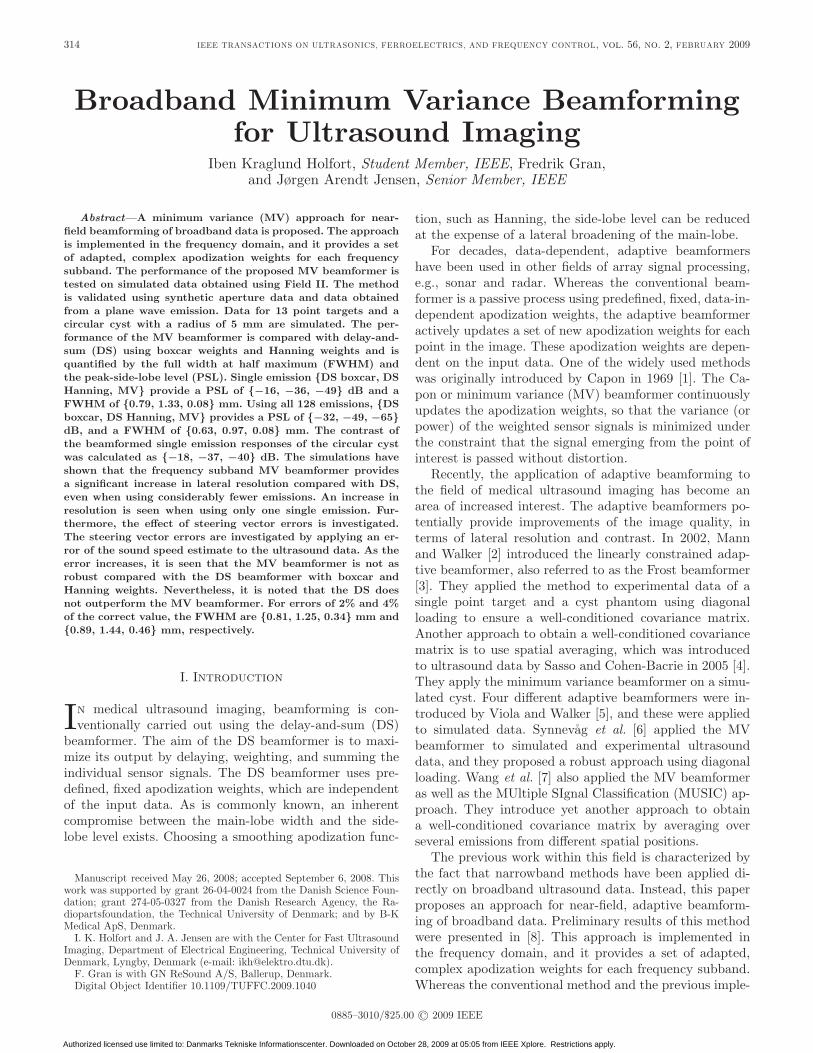
conventionally, beamforming is carried out on each of the sensor signals independently. as shown in Fig. 1, each sensor signal is delayed and weighted; and they are consecutively summed to form the beamformer output. The ds beamformer is a passive process using predefined, fixed, data-independent apodization weights. because the phase-shift can be implemented as a time-delay, the ds beamformer works for both narrowband and broadband signals.

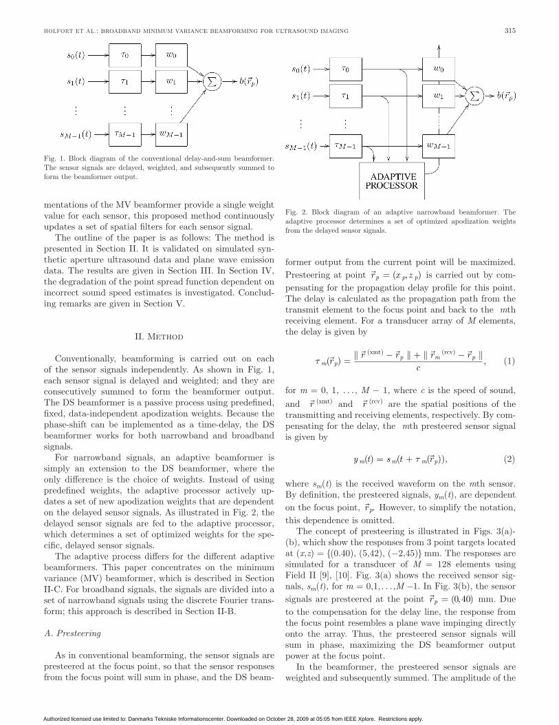
For narrowband signals, an adaptive beamformer is simply an extension to the ds beamformer, where the only difference is the choice of weights. Instead of using predefined weights, the adaptive processor actively up-dates a set of new apodization weights that are dependent on the delayed sensor signals. as illustrated in Fig. 2, the delayed sensor signals are fed to the adaptive processor, which determines a set of optimized weights for the spe-cific, delayed sensor signals.

The adaptive process differs for the different adaptive beamformers. This paper concentrates on the minimum variance (MV) beamformer, which is described in section II-c. For broadband signals, the signals are divided into a set of narrowband signals using the discrete Fourier trans-form; this approach is described in section II-b.

A. Presteering

as in conventional beamforming, the sensor signals are presteered at the focus point, so that the sensor responses from the focus point will sum in phase, and the ds beam-

former output from the current point will be maximized. Presteering at point

r x zp p p= ( , ) is carried out by com-pensating for the propagation delay profile for this point. The delay is calculated as the propagation path from the transmit element to the focus point and back to the mth receiving element. For a transducer array of M elements, the delay is given by

t m pp m pr

r r r rc

( ) ,

=- + -(xmt) (rcv)

(1)

for m = 0, 1, …, M − 1, where c is the speed of sound, and

r (xmt) and

r (rcv) are the spatial positions of the transmitting and receiving elements, respectively. by com-pensating for the delay, the mth presteered sensor signal is given by

y t s t rm m m p( ) ( ( )),= + t

(2)

where sm(t) is the received waveform on the mth sensor. by definition, the presteered signals, ym(t), are dependent on the focus point,

r p. However, to simplify the notation, this dependence is omitted.

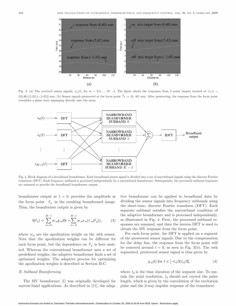
The concept of presteering is illustrated in Figs. 3(a)-(b), which show the responses from 3 point targets located at (x,z) = {(0.40), (5,42), (−2,45)} mm. The responses are simulated for a transducer of M = 128 elements using Field II [9], [10]. Fig. 3(a) shows the received sensor sig-nals, sm(t), for m = 0,1,…,M −1. In Fig. 3(b), the sensor signals are presteered at the point

r p = ( , )0 40 mm. due to the compensation for the delay line, the response from the focus point resembles a plane wave impinging directly onto the array. Thus, the presteered sensor signals will sum in phase, maximizing the ds beamformer output power at the focus point.

In the beamformer, the presteered sensor signals are weighted and subsequently summed. The amplitude of the

315HolForT ET al.: broadband minimum variance beamforming for ultrasound imaging

Fig. 1. block diagram of the conventional delay-and-sum beamformer. The sensor signals are delayed, weighted, and subsequently summed to form the beamformer output.

Fig. 2. block diagram of an adaptive narrowband beamformer. The adaptive processor determines a set of optimized apodization weights from the delayed sensor signals.


beamformer output at t = 0, provides the amplitude at the focus point

r p in the resulting beamformed image. Thus, the beamformer output is given by

b r w y w s rp m mm

M

m m m pm

M

( ) ( ) ( ( )),

= ==

-

-

-

å å00

1

0

1

t (3)

where wm are the apodization weight on the mth sensor. note that the apodization weights can be different for each focus point, but the dependence on

r p is here omit-ted. Whereas the conventional beamformer uses a set of predefined weights, the adaptive beamformer finds a set of optimized weights. The adaptive process for optimizing the apodization weights is described in section II-c.

B. Subband Beamforming

The MV beamformer [1] was originally developed for narrow-band applications. as described in [11], the adap-

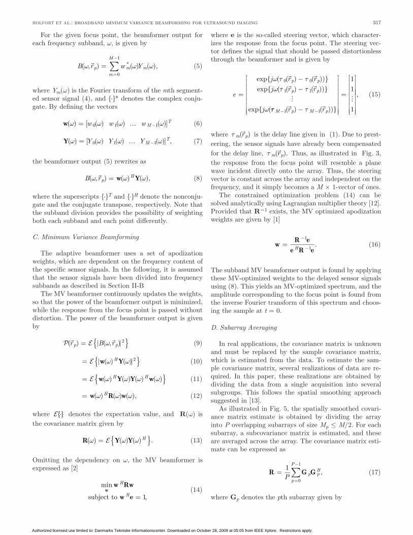
tive beamformer can be applied to broadband data by dividing the sensor signals into frequency subbands using the short-time, discrete Fourier transform (dFT). Each separate subband satisfies the narrowband condition of the adaptive beamformer and is processed independently, as illustrated in Fig. 4. First, the processed subband re-sponses are summed, and then the inverse dFT is used to obtain the MV response from the focus point.

For each focus point, the dFT is applied on a segment of the presteered sensor signals. due to the compensation for the delay line, the response from the focus point will be centered around t = 0, as seen in Fig. 3(b). The mth segmented, presteered sensor signal is thus given by

y t t t tm d d( ) [ ; ], for / /Î - 2 2 (4)

where td is the time duration of the segment size. To sus-tain the axial resolution, td should not exceed the pulse length, which is given by the convolution of the excitation pulse and the 2-way impulse response of the transducer.


Fig. 3. (a) The received sensor signals, sm(t), for m = 0,1,…,M −1. The figure shows the responses from 3 point targets located at (x,z) =

{(0,40),(5,42),(−2,45)} mm. (b) sensor signals presteered at the focus point

r p = (0, 40) mm. after presteering, the response from the focus point resembles a plane wave impinging directly onto the array.

Fig. 4. block diagram of a broadband beamformer. Each broadband sensor signal is divided into a set of narrowband signals using the discrete Fourier transform (dFT). Each frequency subband is processed independently by a narrowband beamformer. subsequently, the processed subband responses are summed to provide the broadband beamformer output.


For the given focus point, the beamformer output for each frequency subband, ω, is given by

B r w Yp m mm

M

( , ) ( ) ( ),*w w w

==

-

å0

1

(5)

where Ym(ω) is the Fourier transform of the mth segment-ed sensor signal (4), and {·}* denotes the complex conju-gate. by defining the vectors

w( ) [ ( ) ( ) ( )]w w w w= ¼ -w w w MT

0 1 1 (6)

Y( ,) [ ( ) ( ) ( )]w w w w= ¼ -Y Y YMT

0 1 1 (7)

the beamformer output (5) rewrites as

B rpH( ( (, ) ) ),w w w

= w Y (8)

where the superscripts {·}T and {·}H denote the nonconju-gate and the conjugate transpose, respectively. note that the subband division provides the possibility of weighting both each subband and each point differently.

C. Minimum Variance Beamforming

The adaptive beamformer uses a set of apodization weights, which are dependent on the frequency content of the specific sensor signals. In the following, it is assumed that the sensor signals have been divided into frequency subbands as described in section II-b

The MV beamformer continuously updates the weights, so that the power of the beamformer output is minimized, while the response from the focus point is passed without distortion. The power of the beamformer output is given by

( ) ( , )

r B rp p= { }| |w 2 (9)

= { } | |w Y( () )w wH 2 (10)

= { } w Y Y w( ( ( () ) ) )w w w wH H (11)

= w R w( ( () ) ),w w wH (12)

where {}× denotes the expectation value, and R(ω) is the covariance matrix given by

R Y Y( ) ) ) .( (w w w= { } H (13)

omitting the dependency on ω, the MV beamformer is expressed as [2]

min

,w

w

w e

RwH

Hsubject to = 1 (14)

where e is the so-called steering vector, which character-izes the response from the focus point. The steering vec-tor defines the signal that should be passed distortionless through the beamformer and is given by

e

j r r

j r r

j

p p

p p=

--

exp{ ( ( ) ( ))}

exp{ ( ( ) ( ))}

exp{ (

w t tw t t

w

0 0

1 1

tt tM p M pr r- --

é

ë

êêêêêêê

ù

û

úúúúúúú

=

é

ë

êêêêêêê

ù

û

úú

1 1

1

1

1( ) ( ))}

úúúúúú

, (15)

where t m pr( )

is the delay line given in (1). due to prest-eering, the sensor signals have already been compensated for the delay line, t m pr( ).

Thus, as illustrated in Fig. 3, the response from the focus point will resemble a plane wave incident directly onto the array. Thus, the steering vector is constant across the array and independent on the frequency, and it simply becomes a M × 1-vector of ones.

The constrained optimization problem (14) can be solved analytically using lagrangian multiplier theory [12]. Provided that R−1 exists, the MV optimized apodization weights are given by [1]

wR e

e R e=

-

-

1

1H. (16)

The subband MV beamformer output is found by applying these MV-optimized weights to the delayed sensor signals using (8). This yields an MV-optimized spectrum, and the amplitude corresponding to the focus point is found from the inverse Fourier transform of this spectrum and choos-ing the sample at t = 0.

D. Subarray Averaging

In real applications, the covariance matrix is unknown and must be replaced by the sample covariance matrix, which is estimated from the data. To estimate the sam-ple covariance matrix, several realizations of data are re-quired. In this paper, these realizations are obtained by dividing the data from a single acquisition into several subgroups. This follows the spatial smoothing approach suggested in [13].

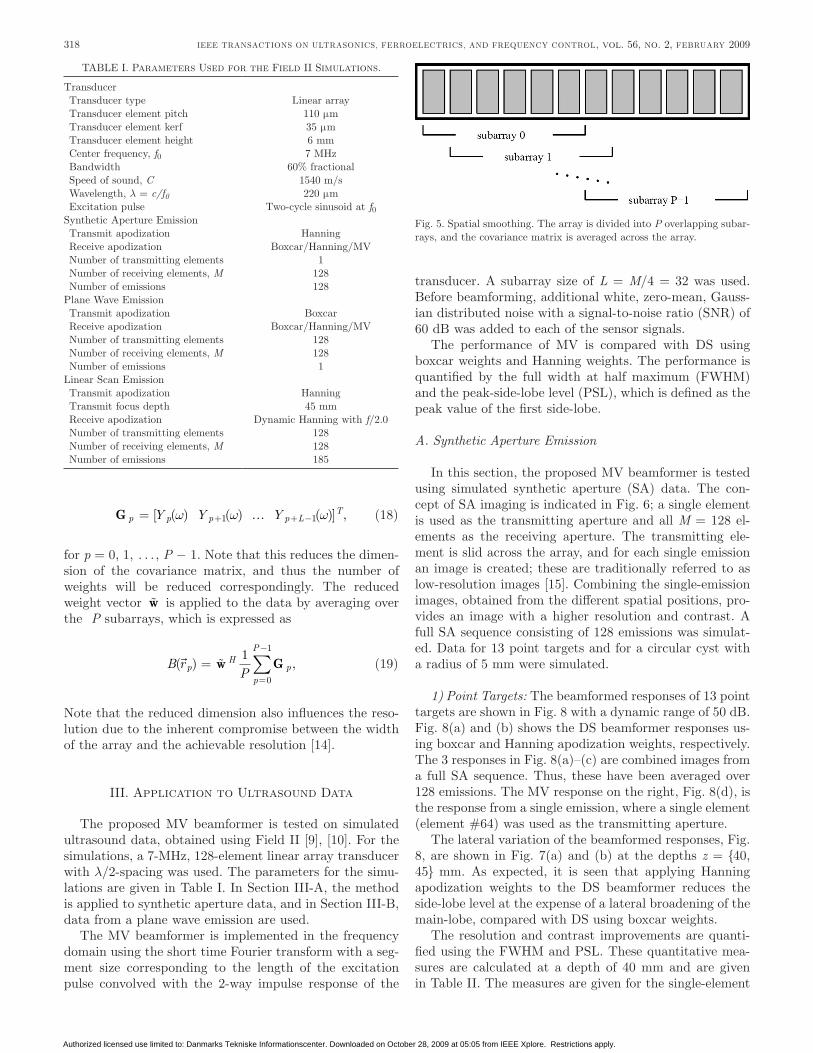
as illustrated in Fig. 5, the spatially smoothed covari-ance matrix estimate is obtained by dividing the array into P overlapping subarrays of size Mp ≤ M/2. For each subarray, a subcovariance matrix is estimated, and these are averaged across the array. The covariance matrix esti-mate can be expressed as

R G G==

-

å1

0

1

P p pH

p

P

, (17)

where Gp denotes the pth subarray given by



G p p p p LTY Y Y= ¼+ + -[ ( ) ( ) ( )] ,w w w1 1 (18)

for p = 0, 1, …, P − 1. note that this reduces the dimen-sion of the covariance matrix, and thus the number of weights will be reduced correspondingly. The reduced weight vector w is applied to the data by averaging over the P subarrays, which is expressed as

B rPp

Hp

p

P

( ) ,

==

-

åw G1

0

1

(19)

note that the reduced dimension also influences the reso-lution due to the inherent compromise between the width of the array and the achievable resolution [14].

III. application to Ultrasound data

The proposed MV beamformer is tested on simulated ultrasound data, obtained using Field II [9], [10]. For the simulations, a 7-MHz, 128-element linear array transducer with λ/2-spacing was used. The parameters for the simu-lations are given in Table I. In section III-a, the method is applied to synthetic aperture data, and in section III-b, data from a plane wave emission are used.

The MV beamformer is implemented in the frequency domain using the short time Fourier transform with a seg-ment size corresponding to the length of the excitation pulse convolved with the 2-way impulse response of the

transducer. a subarray size of L = M/4 = 32 was used. before beamforming, additional white, zero-mean, Gauss-ian distributed noise with a signal-to-noise ratio (snr) of 60 db was added to each of the sensor signals.

The performance of MV is compared with ds using boxcar weights and Hanning weights. The performance is quantified by the full width at half maximum (FWHM) and the peak-side-lobe level (Psl), which is defined as the peak value of the first side-lobe.

A. Synthetic Aperture Emission

In this section, the proposed MV beamformer is tested using simulated synthetic aperture (sa) data. The con-cept of sa imaging is indicated in Fig. 6; a single element is used as the transmitting aperture and all M = 128 el-ements as the receiving aperture. The transmitting ele-ment is slid across the array, and for each single emission an image is created; these are traditionally referred to as low-resolution images [15]. combining the single-emission images, obtained from the different spatial positions, pro-vides an image with a higher resolution and contrast. a full sa sequence consisting of 128 emissions was simulat-ed. data for 13 point targets and for a circular cyst with a radius of 5 mm were simulated.

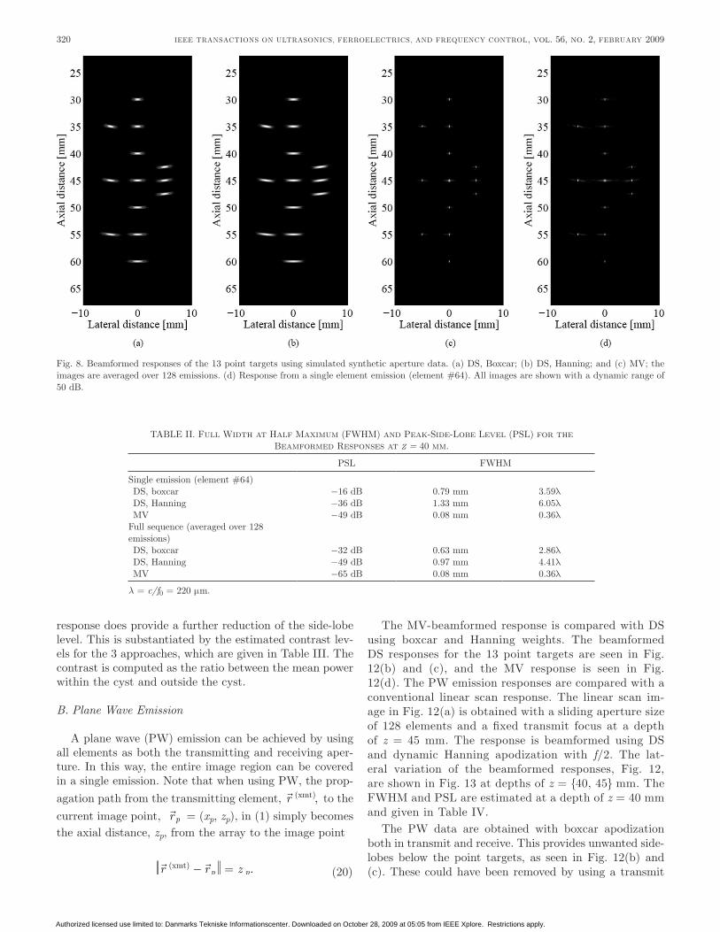
1) Point Targets: The beamformed responses of 13 point targets are shown in Fig. 8 with a dynamic range of 50 db. Fig. 8(a) and (b) shows the ds beamformer responses us-ing boxcar and Hanning apodization weights, respectively. The 3 responses in Fig. 8(a)–(c) are combined images from a full sa sequence. Thus, these have been averaged over 128 emissions. The MV response on the right, Fig. 8(d), is the response from a single emission, where a single element (element #64) was used as the transmitting aperture.

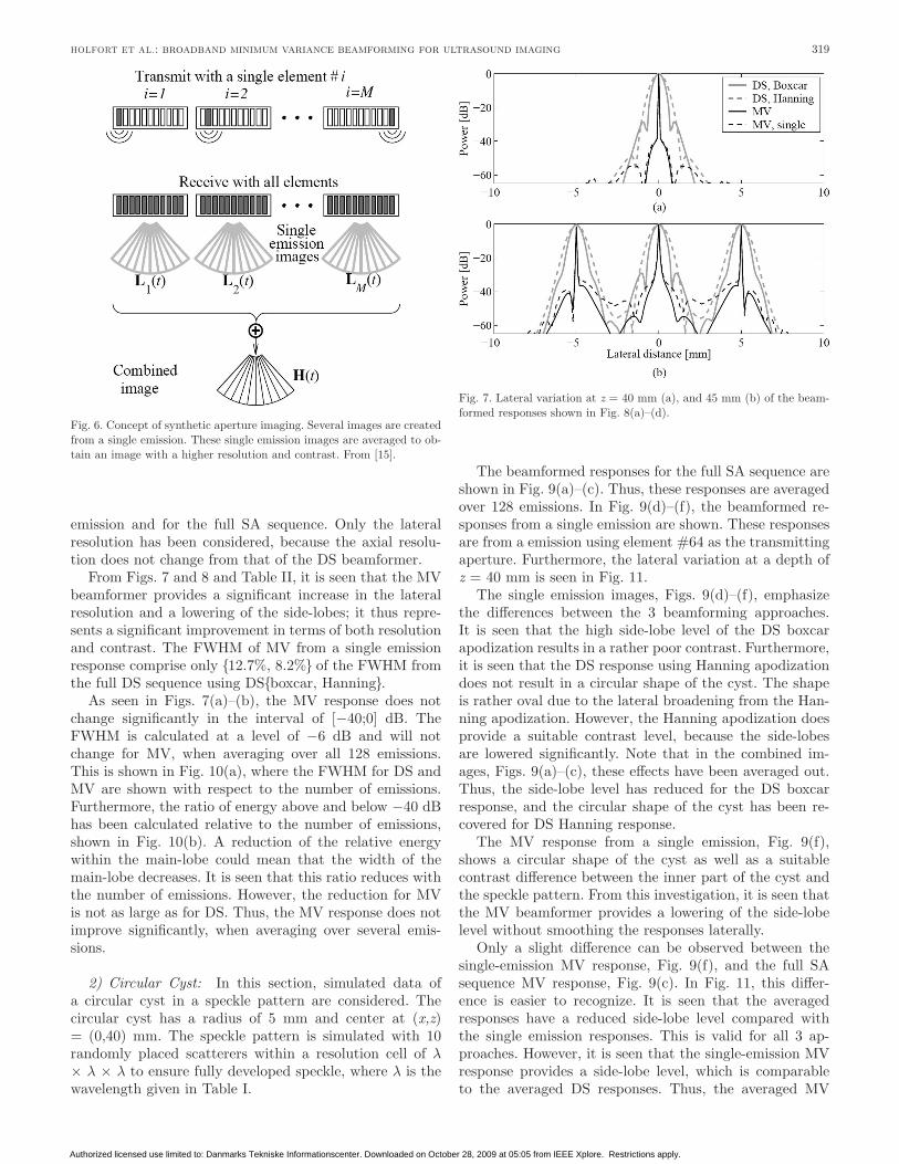
The lateral variation of the beamformed responses, Fig. 8, are shown in Fig. 7(a) and (b) at the depths z = {40, 45} mm. as expected, it is seen that applying Hanning apodization weights to the ds beamformer reduces the side-lobe level at the expense of a lateral broadening of the main-lobe, compared with ds using boxcar weights.

The resolution and contrast improvements are quanti-fied using the FWHM and Psl. These quantitative mea-sures are calculated at a depth of 40 mm and are given in Table II. The measures are given for the single-element


Fig. 5. spatial smoothing. The array is divided into P overlapping subar-rays, and the covariance matrix is averaged across the array.

TablE I. Parameters Used for the Field II simulations.

Transducer Transducer type linear array Transducer element pitch 110 μm Transducer element kerf 35 μm Transducer element height 6 mm center frequency, f0 7 MHz bandwidth 60% fractional speed of sound, C 1540 m/s Wavelength, λ = c/f0 220 μm Excitation pulse Two-cycle sinusoid at f0synthetic aperture Emission Transmit apodization Hanning receive apodization boxcar/Hanning/MV number of transmitting elements 1 number of receiving elements, M 128 number of emissions 128Plane Wave Emission Transmit apodization boxcar receive apodization boxcar/Hanning/MV number of transmitting elements 128 number of receiving elements, M 128 number of emissions 1linear scan Emission Transmit apodization Hanning Transmit focus depth 45 mm receive apodization dynamic Hanning with f/2.0 number of transmitting elements 128 number of receiving elements, M 128 number of emissions 185


emission and for the full sa sequence. only the lateral resolution has been considered, because the axial resolu-tion does not change from that of the ds beamformer.

From Figs. 7 and 8 and Table II, it is seen that the MV beamformer provides a significant increase in the lateral resolution and a lowering of the side-lobes; it thus repre-sents a significant improvement in terms of both resolution and contrast. The FWHM of MV from a single emission response comprise only {12.7%, 8.2%} of the FWHM from the full ds sequence using ds{boxcar, Hanning}.

as seen in Figs. 7(a)–(b), the MV response does not change significantly in the interval of [−40;0] db. The FWHM is calculated at a level of −6 db and will not change for MV, when averaging over all 128 emissions. This is shown in Fig. 10(a), where the FWHM for ds and MV are shown with respect to the number of emissions. Furthermore, the ratio of energy above and below −40 db has been calculated relative to the number of emissions, shown in Fig. 10(b). a reduction of the relative energy within the main-lobe could mean that the width of the main-lobe decreases. It is seen that this ratio reduces with the number of emissions. However, the reduction for MV is not as large as for ds. Thus, the MV response does not improve significantly, when averaging over several emis-sions.

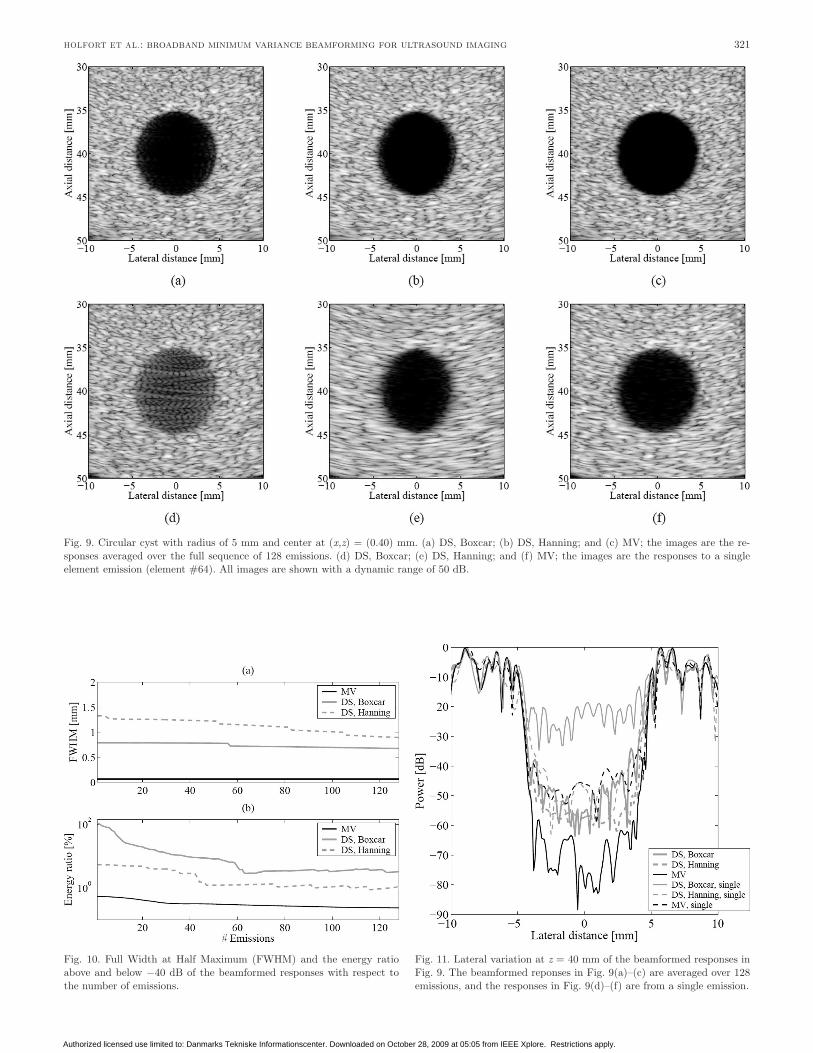
2) Circular Cyst: In this section, simulated data of a circular cyst in a speckle pattern are considered. The circular cyst has a radius of 5 mm and center at (x,z) = (0,40) mm. The speckle pattern is simulated with 10 randomly placed scatterers within a resolution cell of λ × λ × λ to ensure fully developed speckle, where λ is the wavelength given in Table I.

The beamformed responses for the full sa sequence are shown in Fig. 9(a)–(c). Thus, these responses are averaged over 128 emissions. In Fig. 9(d)–(f), the beamformed re-sponses from a single emission are shown. These responses are from a emission using element #64 as the transmitting aperture. Furthermore, the lateral variation at a depth of z = 40 mm is seen in Fig. 11.

The single emission images, Figs. 9(d)–(f), emphasize the differences between the 3 beamforming approaches. It is seen that the high side-lobe level of the ds boxcar apodization results in a rather poor contrast. Furthermore, it is seen that the ds response using Hanning apodization does not result in a circular shape of the cyst. The shape is rather oval due to the lateral broadening from the Han-ning apodization. However, the Hanning apodization does provide a suitable contrast level, because the side-lobes are lowered significantly. note that in the combined im-ages, Figs. 9(a)–(c), these effects have been averaged out. Thus, the side-lobe level has reduced for the ds boxcar response, and the circular shape of the cyst has been re-covered for ds Hanning response.

The MV response from a single emission, Fig. 9(f), shows a circular shape of the cyst as well as a suitable contrast difference between the inner part of the cyst and the speckle pattern. From this investigation, it is seen that the MV beamformer provides a lowering of the side-lobe level without smoothing the responses laterally.

only a slight difference can be observed between the single-emission MV response, Fig. 9(f), and the full sa sequence MV response, Fig. 9(c). In Fig. 11, this differ-ence is easier to recognize. It is seen that the averaged responses have a reduced side-lobe level compared with the single emission responses. This is valid for all 3 ap-proaches. However, it is seen that the single-emission MV response provides a side-lobe level, which is comparable to the averaged ds responses. Thus, the averaged MV


Fig. 6. concept of synthetic aperture imaging. several images are created from a single emission. These single emission images are averaged to ob-tain an image with a higher resolution and contrast. From [15].

Fig. 7. lateral variation at z = 40 mm (a), and 45 mm (b) of the beam-formed responses shown in Fig. 8(a)–(d).


response does provide a further reduction of the side-lobe level. This is substantiated by the estimated contrast lev-els for the 3 approaches, which are given in Table III. The contrast is computed as the ratio between the mean power within the cyst and outside the cyst.

B. Plane Wave Emission

a plane wave (PW) emission can be achieved by using all elements as both the transmitting and receiving aper-ture. In this way, the entire image region can be covered in a single emission. note that when using PW, the prop-agation path from the transmitting element,

r (xmt), to the current image point,

r p = (xp, zp), in (1) simply becomes the axial distance, zp, from the array to the image point

r r zp p(xmt) - = . (20)

The MV-beamformed response is compared with ds using boxcar and Hanning weights. The beamformed ds responses for the 13 point targets are seen in Fig. 12(b) and (c), and the MV response is seen in Fig. 12(d). The PW emission responses are compared with a conventional linear scan response. The linear scan im-age in Fig. 12(a) is obtained with a sliding aperture size of 128 elements and a fixed transmit focus at a depth of z = 45 mm. The response is beamformed using ds and dynamic Hanning apodization with f/2. The lat-eral variation of the beamformed responses, Fig. 12, are shown in Fig. 13 at depths of z = {40, 45} mm. The FWHM and Psl are estimated at a depth of z = 40 mm and given in Table IV.

The PW data are obtained with boxcar apodization both in transmit and receive. This provides unwanted side-lobes below the point targets, as seen in Fig. 12(b) and (c). These could have been removed by using a transmit


TablE II. Full Width at Half Maximum (FWHM) and Peak-side-lobe level (Psl) for the beamformed responses at z = 40 mm.

Psl FWHM

single emission (element #64) ds, boxcar −16 db 0.79 mm 3.59λ ds, Hanning −36 db 1.33 mm 6.05λ MV −49 db 0.08 mm 0.36λFull sequence (averaged over 128 emissions) ds, boxcar −32 db 0.63 mm 2.86λ ds, Hanning −49 db 0.97 mm 4.41λ MV −65 db 0.08 mm 0.36λ

λ = c/f0 = 220 μm.

Fig. 8. beamformed responses of the 13 point targets using simulated synthetic aperture data. (a) ds, boxcar; (b) ds, Hanning; and (c) MV; the images are averaged over 128 emissions. (d) response from a single element emission (element #64). all images are shown with a dynamic range of 50 db.



Fig. 10. Full Width at Half Maximum (FWHM) and the energy ratio above and below −40 db of the beamformed responses with respect to the number of emissions.

Fig. 9. circular cyst with radius of 5 mm and center at (x,z) = (0.40) mm. (a) ds, boxcar; (b) ds, Hanning; and (c) MV; the images are the re-sponses averaged over the full sequence of 128 emissions. (d) ds, boxcar; (e) ds, Hanning; and (f) MV; the images are the responses to a single element emission (element #64). all images are shown with a dynamic range of 50 db.

Fig. 11. lateral variation at z = 40 mm of the beamformed responses in Fig. 9. The beamformed reponses in Fig. 9(a)–(c) are averaged over 128 emissions, and the responses in Fig. 9(d)–(f) are from a single emission.


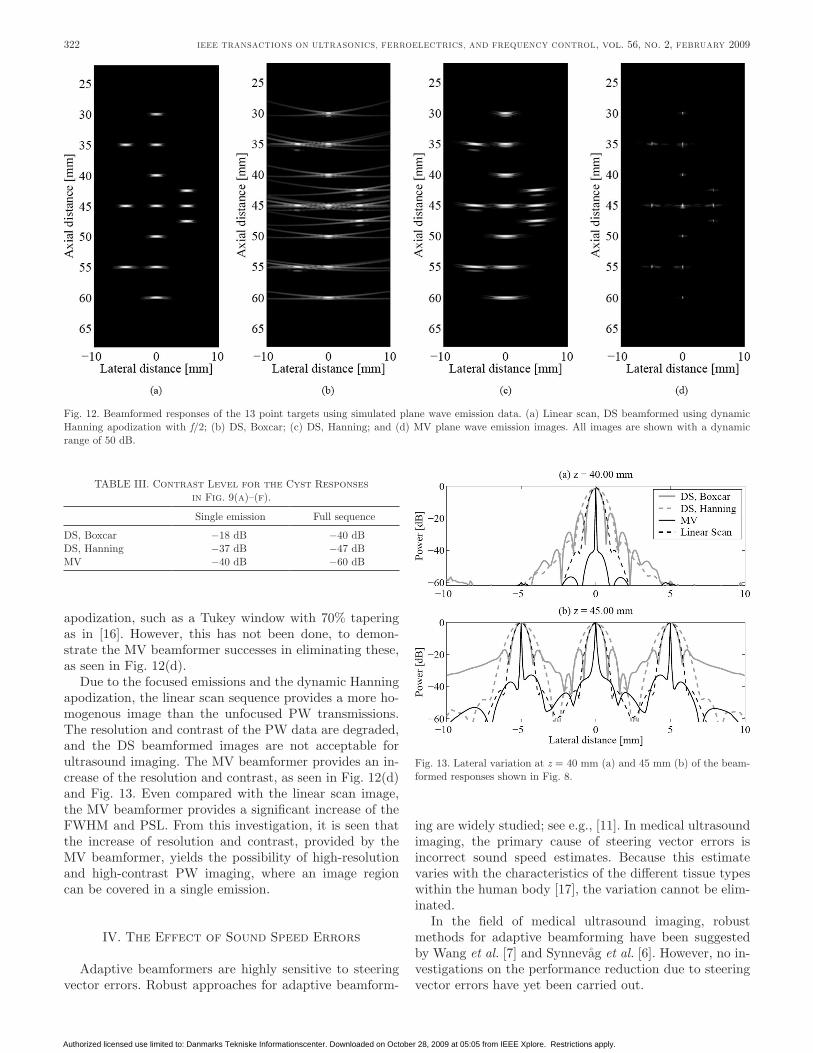
apodization, such as a Tukey window with 70% tapering as in [16]. However, this has not been done, to demon-strate the MV beamformer successes in eliminating these, as seen in Fig. 12(d).

due to the focused emissions and the dynamic Hanning apodization, the linear scan sequence provides a more ho-mogenous image than the unfocused PW transmissions. The resolution and contrast of the PW data are degraded, and the ds beamformed images are not acceptable for ultrasound imaging. The MV beamformer provides an in-crease of the resolution and contrast, as seen in Fig. 12(d) and Fig. 13. Even compared with the linear scan image, the MV beamformer provides a significant increase of the FWHM and Psl. From this investigation, it is seen that the increase of resolution and contrast, provided by the MV beamformer, yields the possibility of high-resolution and high-contrast PW imaging, where an image region can be covered in a single emission.

IV. The Effect of sound speed Errors

adaptive beamformers are highly sensitive to steering vector errors. robust approaches for adaptive beamform-

ing are widely studied; see e.g., [11]. In medical ultrasound imaging, the primary cause of steering vector errors is incorrect sound speed estimates. because this estimate varies with the characteristics of the different tissue types within the human body [17], the variation cannot be elim-inated.

In the field of medical ultrasound imaging, robust methods for adaptive beamforming have been suggested by Wang et al. [7] and synnevåg et al. [6]. However, no in-vestigations on the performance reduction due to steering vector errors have yet been carried out.


TablE III. contrast level for the cyst responses in Fig. 9(a) –(f).

single emission Full sequence

ds, boxcar −18 db −40 dbds, Hanning −37 db −47 dbMV −40 db −60 db

Fig. 12. beamformed responses of the 13 point targets using simulated plane wave emission data. (a) linear scan, ds beamformed using dynamic Hanning apodization with f/2; (b) ds, boxcar; (c) ds, Hanning; and (d) MV plane wave emission images. all images are shown with a dynamic range of 50 db.

Fig. 13. lateral variation at z = 40 mm (a) and 45 mm (b) of the beam-formed responses shown in Fig. 8.


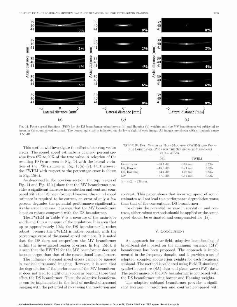
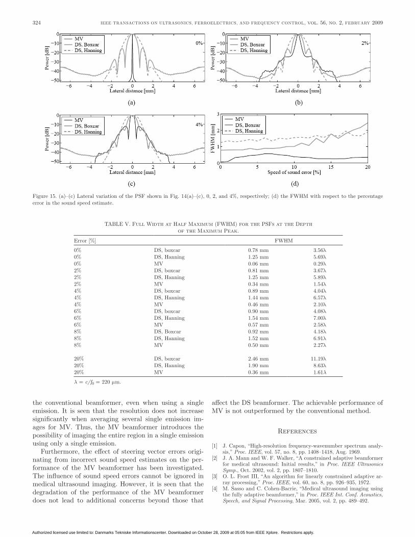
This section will investigate the effect of steering vector errors. The sound speed estimate is changed percentage-wise from 0% to 20% of the true value. a selection of the resulting PsFs are seen in Fig. 14 with the lateral varia-tion of the PsFs shown in Fig. 15(a)–(c). Furthermore, the FWHM with respect to the percentage error is shown in Fig. 15(d).

as described in the previous section, the top images of Fig. 14 and Fig. 15(a) show that the MV beamformer pro-vides a significant increase in resolution and contrast com-pared with the ds beamformer. However, the sound speed estimate is required to be correct, an error of only a few percent degrades the potential performance significantly. as the error increases, it is seen that the MV beamformer is not as robust compared with the ds beamformer.

The FWHM in Table V is a measure of the main-lobe width and thus a measure of the resolution. It is seen that up to approximately 10%, the ds beamformer is rather robust, because the FWHM is rather constant with the percentage error of the sound speed estimate. It is noted that the ds does not outperform the MV beamformer within the investigated region of errors. In Fig. 15(d), it is seen that the FWHM for the MV beamformer does not become larger than that of the conventional beamformer.

The influence of sound speed errors cannot be ignored in medical ultrasound imaging. However, it is seen that the degradation of the performance of the MV beamform-er does not lead to additional concerns beyond those that affect the ds beamformer. Thus, the adaptive beamform-er can be implemented in the field of medical ultrasound imaging with the potential of increasing the resolution and

contrast. This paper shows that incorrect speed of sound estimates will not lead to a performance degradation worse than that of the conventional ds beamformer.

To obtain the potential increase in resolution and con-trast, either robust methods should be applied or the sound speed should be estimated and compensated for [18].

V. conclusions

an approach for near-field, adaptive beamforming of broadband data based on the minimum variance (MV) beamformer has been proposed. The approach is imple-mented in the frequency domain, and it provides a set of adapted, complex apodization weights for each frequency subband. The method is validated using Field II simulated synthetic aperture (sa) data and plane wave (PW) data. The performance of the MV beamformer is compared with the ds beamformer using boxcar and Hanning weights.

The adaptive subband beamformer provides a signifi-cant increase in resolution and contrast compared with


TablE IV. Full Width at Half Maximum (FWHM) and Peak-side lobe level (Psl) for the beamformed responses

at z = 40 mm.

Psl FWHM

linear scan −40.1 db 0.82 mm 3.71λds, boxcar −16.8 db 0.71 mm 3.23λds, Hanning −34.4 db 1.28 mm 5.81λMV −57.0 db 0.12 mm 0.53λ

λ = c/f0 = 220 μm.

Fig. 14. Point spread functions (PsF) for the ds beamformer using boxcar (a) and Hanning (b) weights, and the MV beamformer (c) subjected to errors in the sound speed estimate. The percentage error is indicated on the lower right of each image. all images are shown with a dynamic range of 50 db.


the conventional beamformer, even when using a single emission. It is seen that the resolution does not increase significantly when averaging several single emission im-ages for MV. Thus, the MV beamformer introduces the possibility of imaging the entire region in a single emission using only a single emission.

Furthermore, the effect of steering vector errors origi-nating from incorrect sound speed estimates on the per-formance of the MV beamformer has been investigated. The influence of sound speed errors cannot be ignored in medical ultrasound imaging. However, it is seen that the degradation of the performance of the MV beamformer does not lead to additional concerns beyond those that

affect the ds beamformer. The achievable performance of MV is not outperformed by the conventional method.

references

[1] J. capon, “High-resolution frequency-wavenumber spectrum analy-sis,” Proc. IEEE, vol. 57, no. 8, pp. 1408–1418, aug. 1969.

[2] J. a. Mann and W. F. Walker, “a constrained adaptive beamformer for medical ultrasound: Initial results,” in Proc. IEEE Ultrasonics Symp., oct. 2002, vol. 2, pp. 1807–1810.

[3] o. l. Frost III, “an algorithm for linearly constrained adaptive ar-ray processing,” Proc. IEEE, vol. 60, no. 8, pp. 926–935, 1972.

[4] M. sasso and c. cohen-bacrie, “Medical ultrasound imaging using the fully adaptive beamformer,” in Proc. IEEE Int. Conf. Acoustics, Speech, and Signal Processing, Mar. 2005, vol. 2, pp. 489–492.


Figure 15. (a)–(c) lateral variation of the PsF shown in Fig. 14(a) –(c), 0, 2, and 4%, respectively; (d) the FWHM with respect to the percentage error in the sound speed estimate.

TablE V. Full Width at Half Maximum (FWHM) for the PsFs at the depth of the Maximum Peak.

Error [%] FWHM

0% ds, boxcar 0.78 mm 3.56λ0% ds, Hanning 1.25 mm 5.69λ0% MV 0.06 mm 0.29λ2% ds, boxcar 0.81 mm 3.67λ2% ds, Hanning 1.25 mm 5.89λ 2% MV 0.34 mm 1.54λ4% ds, boxcar 0.89 mm 4.04λ4% ds, Hanning 1.44 mm 6.57λ4% MV 0.46 mm 2.10λ6% ds, boxcar 0.90 mm 4.08λ6% ds, Hanning 1.54 mm 7.00λ6% MV 0.57 mm 2.58λ8% ds, boxcar 0.92 mm 4.18λ8% ds, Hanning 1.52 mm 6.91λ8% MV 0.50 mm 2.27λ

20% ds, boxcar 2.46 mm 11.19λ20% ds, Hanning 1.90 mm 8.63λ20% MV 0.36 mm 1.61λ

λ = c/f0 = 220 μm.


[5] F. Viola and W. F. Walker, “adaptive signal processing in medical ultrasound beamforming,” in Proc. IEEE Ultrasonics Symp., 2005, vol. 4, pp. 1980–1983.

[6] J.-F. synnevåg, a. austeng, and s. Holm, “adaptive beamforming applied to medical ultrasound imaging,” IEEE Trans. Ultrason. Fer-roelectr. Freq. Control, vol. 54, no. 8, pp. 1606–1613, aug. 2007.

[7] Z. Wang, J. li, and r. Wu, “Time-delay- and time-reversal-based robust capon beamformers for ultrasound imaging,” IEEE Trans. Med. Imaging, vol. 24, no. 10, pp. 1308–1322, oct. 2005.

[8] I. K. Holfort, F. Gran, and J. a. Jensen, “Minimum variance beam-forming for high frame-rate ultrasound imaging,” in Proc. IEEE Ultrasonics Symp., oct. 2007, pp. 1541–1544.

[9] J. a. Jensen and n. b. svendsen, “calculation of pressure fields from arbitrarily shaped, apodized, and excited ultrasound transduc-ers,” IEEE Trans. Ultrason. Ferroelectr. Freq. Control, vol. 39, pp. 262–267, Mar. 1992.

[10] J. a. Jensen, “Field: a program for simulating ultrasound systems,” Med. Biol. Eng. Comp., 10th nordic-baltic conference on biomedi-cal Imaging, vol. 4, suppl. 1, part 1, pp. 351–353, 1996b.

[11] J. li and P. stoica, Robust Adaptive Beamforming. new york: John Wiley & sons, 2006.

[12] J. s. arora, Introduction to Optimum Design. new york: McGraw-Hill, Inc., 1989.

[13] T.-J. shan and T. Kailath, “adaptive beamforming for coherent signals and interference,” IEEE Trans. Acoust. Speech. Sig. Pro., vol. 33, no. 3, pp. 527–536, Jun. 1985.

[14] d. H. Johnson and d. E. dudgeon, Array Signal Processing. Con-cepts and Techniques. Englewood cliffs, nJ: Prentice-Hall, 1993.

[15] s. I. nikolov and J. a. Jensen, “In-vivo synthetic aperture flow imaging in medical ultrasound,” IEEE Trans. Ultrason. Ferroelectr. Freq. Control, vol. 50, no. 7, pp. 848–856, 2003.

[16] J. Udesen, F. Gran, and J. a. Jensen, “Fast color flow mode imag-ing using plane wave excitation and temporal encoding,” in Proc. SPIE—Progress in Biomedical Optics and Imaging, 2005, vol. 5750, pp. 427–436.

[17] s. a. Goss, r. l. Johnston, and F. dunn, “comprehensive compila-tion of empirical ultrasonic properties of mammalian tissues,” J. Acoust. Soc. Am., vol. 64, pp. 423–457, aug. 1978.

[18] d. robinson, J. ophir, and c. chen, “Pulse-echo ultrasound speed measurements: Progress and prospects,” Ultrasound Med. Biol., vol. 17, no. 6, pp. 633–646, 1991.

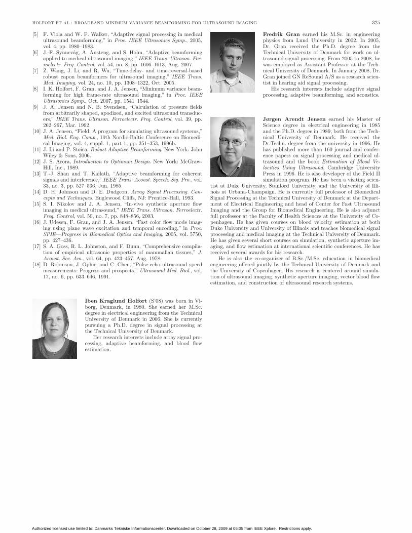
Iben Kraglund Holfort (s’08) was born in Vi-borg, denmark, in 1980. she earned her M.sc. degree in electrical engineering from the Technical University of denmark in 2006. she is currently pursuing a Ph.d. degree in signal processing at the Technical University of denmark.

Her research interests include array signal pro-cessing, adaptive beamforming, and blood flow estimation.

Fredrik Gran earned his M.sc. in engineering physics from lund University in 2002. In 2005, dr. Gran received the Ph.d. degree from the Technical University of denmark for work on ul-trasound signal processing. From 2005 to 2008, he was employed as assistant Professor at the Tech-nical University of denmark. In January 2008, dr. Gran joined Gn resound a/s as a research scien-tist in hearing aid signal processing.

His research interests include adaptive signal processing, adaptive beamforming, and acoustics.

Jørgen Arendt Jensen earned his Master of science degree in electrical engineering in 1985 and the Ph.d. degree in 1989, both from the Tech-nical University of denmark. He received the dr.Techn. degree from the university in 1996. He has published more than 160 journal and confer-ence papers on signal processing and medical ul-trasound and the book Estimation of Blood Ve-locities Using Ultrasound, cambridge University Press in 1996. He is also developer of the Field II simulation program. He has been a visiting scien-

tist at duke University, stanford University, and the University of Illi-nois at Urbana-champaign. He is currently full professor of biomedical signal Processing at the Technical University of denmark at the depart-ment of Electrical Engineering and head of center for Fast Ultrasound Imaging and the Group for biomedical Engineering. He is also adjunct full professor at the Faculty of Health sciences at the University of co-penhagen. He has given courses on blood velocity estimation at both duke University and University of Illinois and teaches biomedical signal processing and medical imaging at the Technical University of denmark. He has given several short courses on simulation, synthetic aperture im-aging, and flow estimation at international scientific conferences. He has received several awards for his research.

He is also the co-organizer of b.sc./M.sc. education in biomedical engineering offered jointly by the Technical University of denmark and the University of copenhagen. His research is centered around simula-tion of ultrasound imaging, synthetic aperture imaging, vector blood flow estimation, and construction of ultrasound research systems.



Documents

Broadband Minimum Variance Beamforming for …orbit.dtu.dk/files/4373217/Holfort.pdfBroadband Minimum Variance Beamforming for Ultrasound Imaging Iben Kraglund Holfort, Student Member,