AUGUST, 2014 BUILDING MINIMUM VARIANCE PORTFOLIOS WITH · PDF fileINNOVATIVE. GLOBAL. INDICES. AUGUST, 2014 BUILDING MINIMUM VARIANCE PORTFOLIOS WITH LOW RISK, LOW DRAWDOWNS AND STRONG

INNOVATIVE. GLOBAL. INDICES.

AUGUST, 2014

BUILDING MINIMUM VARIANCE PORTFOLIOS WITH LOW RISK, LOW DRAWDOWNS AND STRONG RETURNS By Ruben Feldman, director business development, STOXX Ltd.

STOXX LIMITED

TABLE OF CONTENTS

Introduction 4

1 Overview of minimum variance investing 5

2 Characteristics of a minimum variance portfolio (MVP) 7

3 Why minimum variance portfolios provide better risk-adjusted returns 9

4 Methodology of STOXX Minimum Variance Indices, highlighting the unique approach for the index series 11

5 A tale of two minimum variance indices 14

6 Minimum variance performance 18

7 Putting the STOXX Minimum Variance indices to use 22

8 Conclusion 27

9 Appendix 28

STOXX LIMITED

TABLE OF FIGURES

FIGURE 1: EFFICIENT FRONTIER OF FEASIBLE PORTFOLIOS. 5

FIGURE 2: ANNUAL RETURNS OF THE STOXX GLOBAL MINIMUM VARIANCE INDICES. 6

FIGURE 3: ACTIVE EXPOSURES TO STYLE FACTORS OF THE STOXX GLOBAL 1800 MINIMUM VARIANCE UNCONSTRAINED RELATIVE TO THE STOXX GLOBAL 1800. 8

FIGURE 4: DISTRIBUTION OF RETURNS FOR A LOW RISK WEIGHTED INDEX AS WELL AS AN MVP COMPARED TO THE BENCHMARK. 11

FIGURE 5: PERFORMANCE OF MINIMUM VARIANCE AND LOW RISK WEIGHTING IN EUROPE. 12

FIGURE 6: FTSE USA MINIMUM VARIANCE IS OPTIMIZED USING A HISTORICAL COVARIANCE APPROACH. THE STOXX INDICES USE A FACTOR MODEL APPROACH. 15

FIGURE 7: THE DAILY AVERAGE OF PREDICTED RISK FOR THE SAME PORTFOLIO, BUT WITH VARYING FREQUENCIES FOR THE STOXX EUROPE 600 MINIMUM VARIANCE. 17

FIGURE 8: PERFORMANCE OF MINIMUM VARIANCE IN BULL AND BEAR MARKETS. 19

FIGURE 9: ACTIVE INDUSTRY EXPOSURE OF THE GLOBAL 1800 MINIMUM VARIANCE UNCONSTRAINED RELATIVE TO THE STOXX GLOBAL 1800. 20

FIGURE 10: MINIMUM VARIANCE’S EXPOSURE TO FINANCIAL SERVICES THROUGH TIME. 21

FIGURE 11: THE EFFECT OF ADDING SATELLITE INVESTMENTS WHILE KEEPING A BETA OF 1. 23

FIGURE 12: STOXX DAILY DATA FROM JAN. 2, 2004 TO MAY 30, 2014 FOR USD GROSS RETURN VERSIONS. A RISK FREE RATE OF 0% WAS USED FOR THE SHARPE RATIO CALCULATION. 24

FIGURE 13: THE EFFECT OF ADDING A MINIMUM VARIANCE SATELLITE TO AN ALREADY DIVERSIFIED PORTFOLIO. 25

FIGURE 14: EFFICIENT FRONTIER USING THREE ASSETS: BARCLAYS CAPITAL BOND COMPOSITE INDEX, STOXX GLOBAL 1800, STOXX GLOBAL 1800 MINIMUM VARIANCE UNCONSTRAINED. 26

STOXX LIMITED

STOXX MINIMUM VARIANCE INDICES

4

Introduction

In the wake of the global financial crisis, minimum variance equity strategies quickly gained traction by capturing the attention of a risk-aware and risk-averse investment community. But minimum variance portfolios (MVPs) offer much more than just an efficient way to lower portfolio volatility. For a growing number of investors, MVPs are now seen as delivering the “best of all worlds”: low risk, low drawdowns and strong returns. While the popularity of these strategies has been markedly more pronounced in recent years, it should be recognized that minimum variance has been in the market for decades. The theory from which the strategy derives its legitimacy is Harry Markowitz’s seminal work published in 1952, which was recognized by the Nobel Prize committee in 19901. The practical importance of low volatility has been championed by R. Haugen and A. J. Heins2 since the mid-1970s, when it started to challenge the generally accepted paradigm of the Efficient Market Hypothesis of E. Fama3. Despite extensive academic research supporting the use of minimum variance, adoption of this strategy is still in the beginning stages. Important practical questions must be answered to provide clarity in the industry. With the focus on reduction of risk, it is natural to assume that there is a return trade off; however there is much academic research and increasing empirical evidence that a minimum variance portfolio provides strong historical total returns and Sharpe ratios. This evidence has seen the MVP become much more commonplace across the marketplace, with momentum growing among institutional investors, mutual funds and ETF sponsors. STOXX has partnered with Axioma to create innovative minimum variance indices that start with a representative STOXX equity index and use Axioma’s multi-factor risk models to estimate a covariance matrix and the Axioma optimization tool to construct the optimal minimum variance index. Since this paper provides an introduction to the STOXX Minimum Variance Indices, we aim to achieve three things:

i) an overview of minimum variance investing ii) the methodology for the construction and maintenance of the STOXX Minimum Variance

Indices, highlighting the unique approach for the index series iii) how investors can make use of the minimum variance concept

1 Markowitz, H. (1952), “Portfolio Selection”, The Journal of Finance, Vol. 7, No. 1 (Mar., 1952), pp. 77-91.

2 Haugen, R. A.; Heins, A. J. (1972), “On the Evidence Supporting the Existence of Risk Premiums in the Capital Market”, University of Wisconsin-

Madison. 3 E. F. Fama, (1965) “The Behavior of Stock-Market Prices” Journal of Business (January, 1965).

STOXX LIMITED


5

1 Overview of minimum variance investing

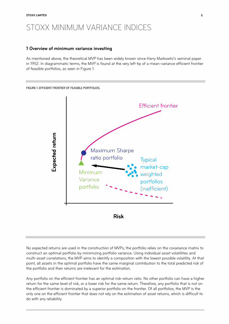
As mentioned above, the theoretical MVP has been widely known since Harry Markowtiz’s seminal paper in 1952. In diagrammatic terms, the MVP is found at the very left tip of a mean-variance efficient frontier of feasible portfolios, as seen in Figure 1.

FIGURE 1: EFFICIENT FRONTIER OF FEASIBLE PORTFOLIOS.

No expected returns are used in the construction of MVPs; the portfolio relies on the covariance matrix to construct an optimal portfolio by minimizing portfolio variance. Using individual asset volatilities and multi-asset correlations, the MVP aims to identify a composition with the lowest possible volatility. At that point, all assets in the optimal portfolio have the same marginal contribution to the total predicted risk of the portfolio and their returns are irrelevant for the estimation. Any portfolio on the efficient frontier has an optimal risk-return ratio. No other portfolio can have a higher return for the same level of risk, or a lower risk for the same return. Therefore, any portfolio that is not on the efficient frontier is dominated by a superior portfolio on the frontier. Of all portfolios, the MVP is the only one on the efficient frontier that does not rely on the estimation of asset returns, which is difficult to do with any reliability.

STOXX LIMITED


6

Although no expected returns are needed to create MVPs, there are three important inputs that are needed:

i) a forecast of variances and covariances ii) an optimization engine iii) a set of constraints that ensures the portfolio is reasonably investable

More details of the approach taken can be found in the next section. The performance characteristics of the MVP can be seen in the chart below:

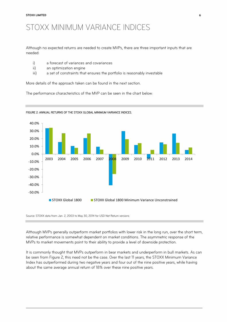
FIGURE 2: ANNUAL RETURNS OF THE STOXX GLOBAL MINIMUM VARIANCE INDICES.

Source: STOXX data from Jan. 2, 2003 to May 30, 2014 for USD Net Return versions

Although MVPs generally outperform market portfolios with lower risk in the long run, over the short term, relative performance is somewhat dependent on market conditions. The asymmetric response of the MVPs to market movements point to their ability to provide a level of downside protection. It is commonly thought that MVPs outperform in bear markets and underperform in bull markets. As can be seen from Figure 2, this need not be the case. Over the last 11 years, the STOXX Minimum Variance Index has outperformed during two negative years and four out of the nine positive years, while having about the same average annual return of 18% over these nine positive years.

-50.0%

-40.0%

-30.0%

-20.0%

-10.0%

0.0%

10.0%

20.0%

30.0%

40.0%

2003 2004 2005 2006 2007 2008 2009 2010 2011 2012 2013 2014

STOXX Global 1800 STOXX Global 1800 Minimum Variance Unconstrained

STOXX LIMITED


7

2 Characteristics of a minimum variance portfolio (MVP)

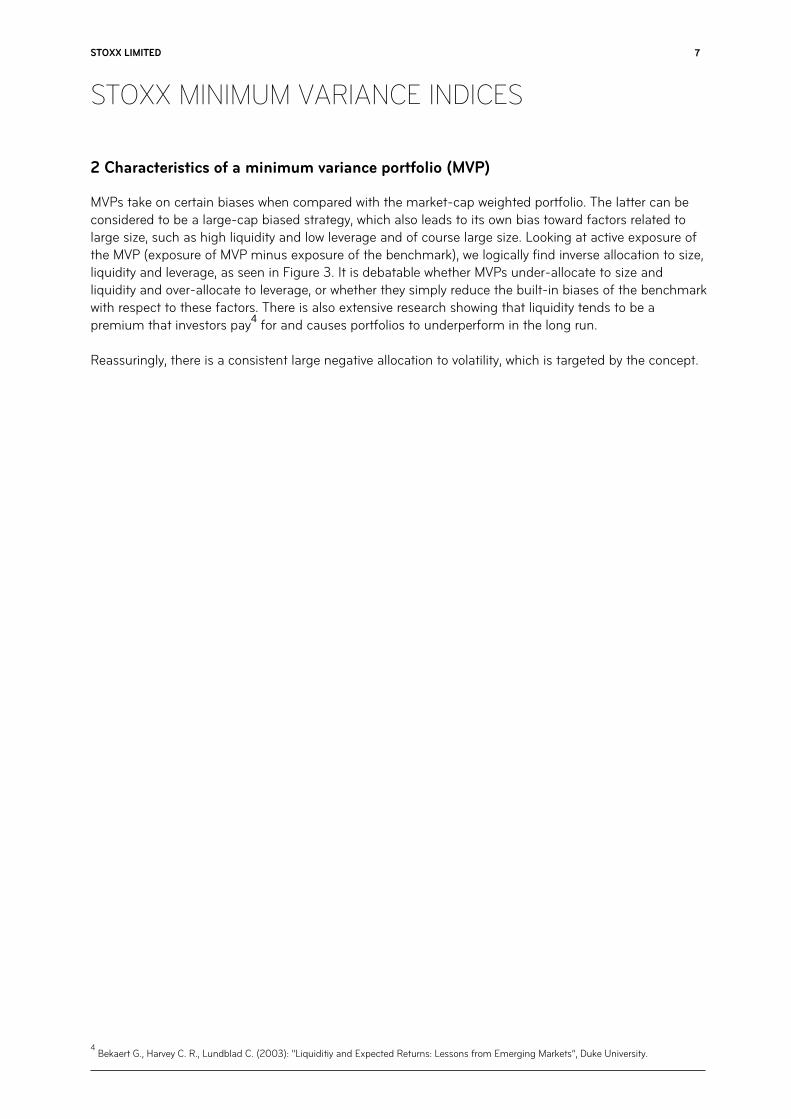
MVPs take on certain biases when compared with the market-cap weighted portfolio. The latter can be considered to be a large-cap biased strategy, which also leads to its own bias toward factors related to large size, such as high liquidity and low leverage and of course large size. Looking at active exposure of the MVP (exposure of MVP minus exposure of the benchmark), we logically find inverse allocation to size, liquidity and leverage, as seen in Figure 3. It is debatable whether MVPs under-allocate to size and liquidity and over-allocate to leverage, or whether they simply reduce the built-in biases of the benchmark with respect to these factors. There is also extensive research showing that liquidity tends to be a premium that investors pay

4 for and causes portfolios to underperform in the long run.

Reassuringly, there is a consistent large negative allocation to volatility, which is targeted by the concept.

4 Bekaert G., Harvey C. R., Lundblad C. (2003): “Liquiditiy and Expected Returns: Lessons from Emerging Markets”, Duke University.

STOXX LIMITED


8

FIGURE 3: ACTIVE EXPOSURES TO STYLE FACTORS OF THE STOXX GLOBAL 1800 MINIMUM VARIANCE UNCONSTRAINED RELATIVE TO THE

STOXX GLOBAL 1800.

Source: STOXX monthly data from Dec. 1999 to Apr. 2014. Factors shown are the standard Axioma style factors.

0.0%

0.2%

0.4%

0.6%

0.8%

1.0%

1.2%

1.4%

1.6%

1.8%

2.0%

Dec

-99

Ap

r-00

Au

g-00

Dec

-00

Ap

r-01

Au

g-01

Dec

-01

Ap

r-02

Au

g-02

Dec

-02

Ap

r-03

Au

g-03

Dec

-03

Ap

r-04

Au

g-04

Dec

-04

Ap

r-05

Au

g-05

Dec

-05

Ap

r-06

Au

g-06

Dec

-06

Ap

r-07

Au

g-07

Dec

-07

Ap

r-08

Au

g-08

Dec

-08

Ap

r-09

Au

g-09

Dec

-09

Ap

r-10

Au

g-10

Dec

-10

Ap

r-11

Au

g-11

Dec

-11

Ap

r-12

Au

g-12

Dec

-12

Ap

r-13

Au

g-13

Dec

-13

Ap

r-14

Volatility

Value

Size

Short-termmomentumMedium-termmomentumLiquidity

Leverage

Growth

Exchange ratesensitivity

-3.5%

-3.0%

-2.5%

-2.0%

-1.5%

-1.0%

-0.5%

0.0% Dec

-99

Ap

r-00

Au

g-00

Dec

-00

Ap

r-01

Au

g-01

Dec

-01

Ap

r-02

Au

g-02

Dec

-02

Ap

r-03

Au

g-03

Dec

-03

Ap

r-04

Au

g-04

Dec

-04

Ap

r-05

Au

g-05

Dec

-05

Ap

r-06

Au

g-06

Dec

-06

Ap

r-07

Au

g-07

Dec

-07

Ap

r-08

Au

g-08

Dec

-08

Ap

r-09

Au

g-09

Dec

-09

Ap

r-10

Au

g-10

Dec

-10

Ap

r-11

Au

g-11

Dec

-11

Ap

r-12

Au

g-12

Dec

-12

Ap

r-13

Au

g-13

Dec

-13

Ap

r-14

Volatility

Value

Size

Short-termmomentumMedium-termmomentumLiquidity

Leverage

Growth

Exchange ratesensitivity

STOXX LIMITED


9

3 Why minimum variance portfolios provide better risk-adjusted returns

MVPs tend to strongly outperform market-cap. weighted portfolios while reducing risk in the long term. In order to trust that this trend will continue and is not just a stroke of luck, it is important to understand the fundamental reasons for this behavior, especially as it contradicts the popular belief that more risk will lead to more returns, as per the CAPM5. First and foremost, we clarify that this behavior is not completely contradictory to the CAPM, as the market-cap weighted index is not necessarily the “market portfolio”. More work would be needed to show this in detail but that is not the focus of this paper. Therefore market-cap weighted portfolios take on some diversifiable risk which is not remunerated by any risk premium. MVPs, in theory, do not take on these risks and so benefit from lower risk while not reducing returns. However, this alone does not explain outperformance. The low volatility anomaly has been defined as “among the many candidates for the greatest anomaly in finance”

6 and many papers have been written attempting to explain the phenomenon. While it is unclear

if a ‘smoking gun’ has been discovered to explain the anomaly, there are many potential reasons that have been extensively discussed.

i) Delegated portfolio management (agency pricing) Because of the way the asset management industry is laid out, portfolio managers often have a greater utility from profit than from loss, for example, through the application of performance fees. Therefore volatile stocks are often sought out in pursuit of greater profits while somewhat neglecting the downside risk. This can lead to an overpricing of volatile assets, which causes underperformance and hence outperformance of less volatile assets.

ii) Leverage aversion

Many investors are not able to leverage. This can lead them to take on higher risk securities in order to achieve target returns. This effect also leads to overpricing volatile stocks.

iii) Tracking error focus

As managers continue to focus on tracking error as a key measurement of success, any asset that takes them away from the benchmark becomes high risk. Therefore, low risk becomes high risk and managers avoid low risk assets, leading to their underpricing as well as crowding in specific assets. This crowding effect not only increases the pricing risk of these assets but also increases their correlation.

iv) Get rich quick

Investors looking for quick returns flock to buy the most volatile assets, leading to overpricing – otherwise known as the ‘lottery ticket effect’.

5 Sharpe, William F. 1964. “Capital Asset Prices: A Theory of Market Equilibrium under Conditions of Risk”. Journal of Finance. 19:3, pp. 425-442.

6 Baker M., Bradley B., Wurgler J. (2011). ”Benchmarks as Limits to Arbitrage: Understanding the Low-Volatility Anomaly”. Financial Analyst

JournaI.

STOXX LIMITED


10

v) The winners curse/jumping on the bandwagon As certain assets achieve exceptional returns, they often get more attention, especially when these returns are quick and thus volatile. This gain in attention often increases its volatility even further as more investors trade it. Investors seeing a good performance sometimes jump on the bandwagon to benefit from a potential upside, often neglecting intrinsic values. This leads to the overpricing of increased volatility stocks.

vi) Neglect

Many high profile stocks garner media attention, while some of the more ‘boring’ assets are overlooked. These higher profile stocks tend to be more volatile as many investors trade them more often than necessary. This is another link between high volatility and overpricing.

vii) Expectations and its risk implications

Companies with higher expectations will most likely have higher volatility as investor response to results will be more severe. The higher the expectations, the higher the chance of investor disappointment.

These behaviors describe how there tends to be a strong relationship between volatility and overpricing. Furthermore, that there are reasons for risky assets to be more highly correlated with each other. MVPs seek to minimize risk. Therefore they will tend to go for lower volatility assets, while reducing allocation to those assets that are highly correlated. In doing this, MVPs select assets that may be underpriced. As this underpricing is reduced and the components become more volatile and correlated to other assets, their weight is reduced in the MVP and may even be phased out. In this process, the MVP has achieved outperformance. When looking at some of the proposed reasons why the MVP outperforms, one observes that the current structure of the market and some fairly fundamental human instincts are behind the success of this strategy. Delegated mandates, tracking error and leverage aversion are unlikely to disappear from the market any time soon. Investor behaviors such as neglect, ‘get rich quick’ and ‘jumping on the bandwagon’ are equally unlikely to vanish. Consequently, it is unlikely that the market will arbitrage away the strategy of the MVP any time soon.

STOXX LIMITED


11

4 Methodology of STOXX Minimum Variance Indices, highlighting the unique approach for the index series

As the minimum variance concept has grown in importance, indices have been created to reflect the concept and to allow benchmarking, as well as to provide cheap access to this strategy for market participants. There are two types of indices on the market:

i) Simple volatility measures ii) Optimized portfolios

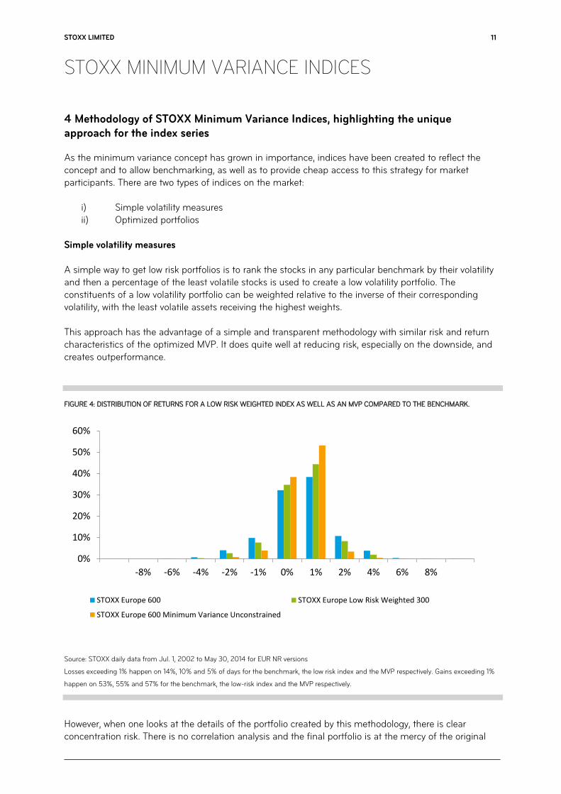
Simple volatility measures A simple way to get low risk portfolios is to rank the stocks in any particular benchmark by their volatility and then a percentage of the least volatile stocks is used to create a low volatility portfolio. The constituents of a low volatility portfolio can be weighted relative to the inverse of their corresponding volatility, with the least volatile assets receiving the highest weights. This approach has the advantage of a simple and transparent methodology with similar risk and return characteristics of the optimized MVP. It does quite well at reducing risk, especially on the downside, and creates outperformance.

FIGURE 4: DISTRIBUTION OF RETURNS FOR A LOW RISK WEIGHTED INDEX AS WELL AS AN MVP COMPARED TO THE BENCHMARK.

Source: STOXX daily data from Jul. 1, 2002 to May 30, 2014 for EUR NR versions

Losses exceeding 1% happen on 14%, 10% and 5% of days for the benchmark, the low risk index and the MVP respectively. Gains exceeding 1%

happen on 53%, 55% and 57% for the benchmark, the low-risk index and the MVP respectively.

However, when one looks at the details of the portfolio created by this methodology, there is clear concentration risk. There is no correlation analysis and the final portfolio is at the mercy of the original

0%

10%

20%

30%

40%

50%

60%

-8% -6% -4% -2% -1% 0% 1% 2% 4% 6% 8%

STOXX Europe 600 STOXX Europe Low Risk Weighted 300

STOXX Europe 600 Minimum Variance Unconstrained

STOXX LIMITED


12

benchmark composition. If a stock in the benchmark was to split into three separate but identical companies, each with the same risk, the low risk weighted portfolio would now assign a weight three times as important, without legitimate justification. This can lead to some concentration risks. In an analysis of the Powershares S&P500® Low Volatility ETF that tracks the S&P500® Low Volatility index many of these concentrations come to light:

- close to 60% of the portfolio was found to be invested in utilities and consumer staples sectors - a strong small-cap bias - A low liquidity bias

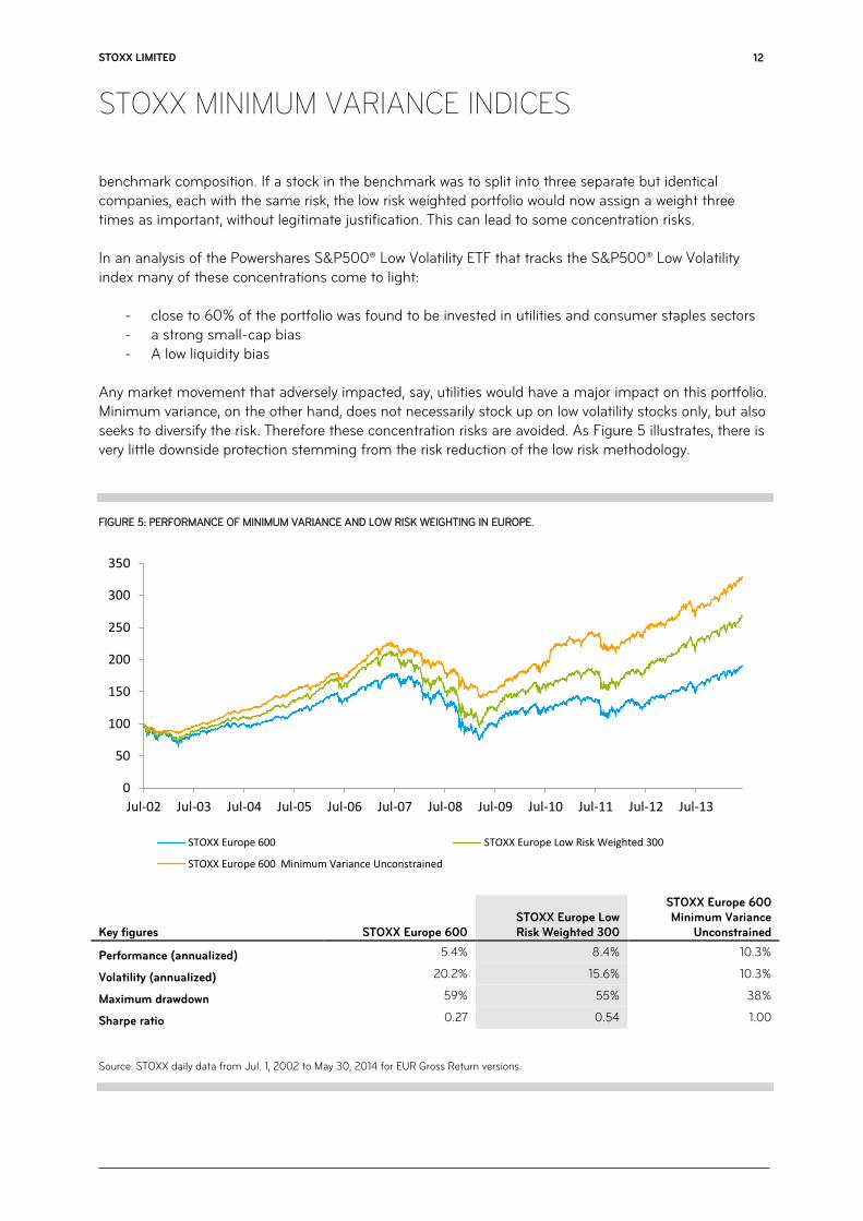
Any market movement that adversely impacted, say, utilities would have a major impact on this portfolio. Minimum variance, on the other hand, does not necessarily stock up on low volatility stocks only, but also seeks to diversify the risk. Therefore these concentration risks are avoided. As Figure 5 illustrates, there is very little downside protection stemming from the risk reduction of the low risk methodology.

FIGURE 5: PERFORMANCE OF MINIMUM VARIANCE AND LOW RISK WEIGHTING IN EUROPE.

Key figures STOXX Europe 600 STOXX Europe Low Risk Weighted 300

STOXX Europe 600 Minimum Variance

Unconstrained

Performance (annualized) 5.4% 8.4% 10.3%

Volatility (annualized) 20.2% 15.6% 10.3%

Maximum drawdown 59% 55% 38%

Sharpe ratio 0.27 0.54 1.00

Source: STOXX daily data from Jul. 1, 2002 to May 30, 2014 for EUR Gross Return versions.

0

50

100

150

200

250

300

350

Jul-02 Jul-03 Jul-04 Jul-05 Jul-06 Jul-07 Jul-08 Jul-09 Jul-10 Jul-11 Jul-12 Jul-13

STOXX Europe 600 STOXX Europe Low Risk Weighted 300

STOXX Europe 600 Minimum Variance Unconstrained

STOXX LIMITED


13

Although the low risk weighting approach does quite well at reducing risk and improving returns, it is not a genuine risk-reduction methodology, as it is subject to the composition of the benchmark. By this we mean that it may have unexpected behavior in certain markets or certain times and it cannot be counted upon to consistently reduce risk. As the results in Figures 4 and 5 suggest, minimum variance does a more consistent job at reducing risk. We see that the distribution of returns is even more desirable using a minimum variance index than a simple risk-reduction strategy. Drawdowns are smaller and occur less often for the MVP and it has a higher average return. The market-cap weighted benchmark has fatter tails.

STOXX LIMITED


14

5 A tale of two minimum variance indices

The STOXX Minimum Variance Indices provide market participants with an easy way to track MVPs in specific markets. For each market – global, regional and country-specific – two versions are made available: Constrained and Unconstrained. The Unconstrained version is optimized with minimal constraints pertaining to tradability and investability and aims to be on the efficient frontier. The Constrained version seeks to also reduce different risks: peer and benchmark risks. By making this second version more constrained to match the market index in terms of risk exposures, it reduces peer and benchmark risks while providing a much improved risk profile (and also returns, for reasons explained previously). The optimization For any minimum variance index, we start with a market-cap weighted broad index, which is supposed to cover about 90% of the market cap of the investment universe. Using this index as a starting selection universe, we apply a constrained optimization to obtain the set of weights for which the portfolio is the smallest possible (something is missing here are we saying … the set of weights which is the smallest possible for the portfolio), while satisfying all the constraints. In order to minimize risk, we must estimate it. There are generally two ways of estimating the covariance of a portfolio: simple historical covariance or using a factor model. Using the historical covariance approach, if we take the STOXX Global 1800 portfolio as an example, we need to create a matrix, C, of size 1,800 by 1,800, which shows the 1,618,200 different pairwise covariances:

Where w is the vector of weights. This is a huge number of parameters to estimate and thus will require us to go very far back in time to obtain sufficient observations to estimate all the parameters (more than 1,800 days or seven years). Furthermore, each day only provides 1,800 observations as only the concerned stocks’ time series are considered. We are therefore doing a lot with little information, yielding poor predictive power. STOXX has teamed up with Axioma to implement a superior methodology. We use Axioma’s fundamental factor model to estimate risk effectively. In this framework, the exposure of each stock to each factor is estimated by the model, and so the covariance of two stocks is determined indirectly through their individual exposures to the factors:

Where E is the matrix of exposures of the stocks to the factors, and F is the covariance matrix of the factors and S represents the residual specific variances. Note that if there are 50 relevant factors, this yields a problem of size 1,800 by 50 and not 1,800 squared as per the historical covariance approach. Thus the problem does not scale exponentially and dealing with a decent universe size is possible. Many implementations of the historical covariance approach slice the starting universe to obtain a more manageable portfolio size. However an optimal solution on a reduced universe will always yield a result that is the same or inferior.

STOXX LIMITED


15

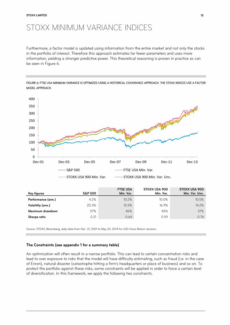
Furthermore, a factor model is updated using information from the entire market and not only the stocks in the portfolio of interest. Therefore this approach estimates far fewer parameters and uses more information, yielding a stronger predictive power. This theoretical reasoning is proven in practice as can be seen in Figure 6.

FIGURE 6: FTSE USA MINIMUM VARIANCE IS OPTIMIZED USING A HISTORICAL COVARIANCE APPROACH. THE STOXX INDICES USE A FACTOR

MODEL APPROACH.

Key figures S&P 500 FTSE USA

Min. Var. STOXX USA 900

Min. Var. STOXX USA 900

Min. Var. Unc.

Performance (ann.) 4.2% 10.2% 10.0% 10.5%

Volatility (ann.) 20.3% 15.9% 16.9% 14.2%

Maximum drawdown 57% 46% 45% 37%

Sharpe ratio 0.21 0.64 0.59 0.74

Source: STOXX, Bloomberg, daily data from Dec. 31, 2001 to May 30, 2014 for USD Gross Return versions.

The Constraints (see appendix 1 for a summary table)

An optimization will often result in a narrow portfolio. This can lead to certain concentration risks and lead to over exposure to risks that the model will have difficulty estimating, such as fraud (i.e. in the case of Enron), natural disaster (catastrophe hitting a firm’s headquarters or place of business) and so on. To protect the portfolio against these risks, some constraints will be applied in order to force a certain level of diversification. In this framework, we apply the following two constraints.

0

50

100

150

200

250

300

350

400

Dec-01 Dec-03 Dec-05 Dec-07 Dec-09 Dec-11 Dec-13

S&P 500 FTSE USA Min. Var.

STOXX USA 900 Min. Var. STOXX USA 900 Min. Var. Unc.

STOXX LIMITED


16

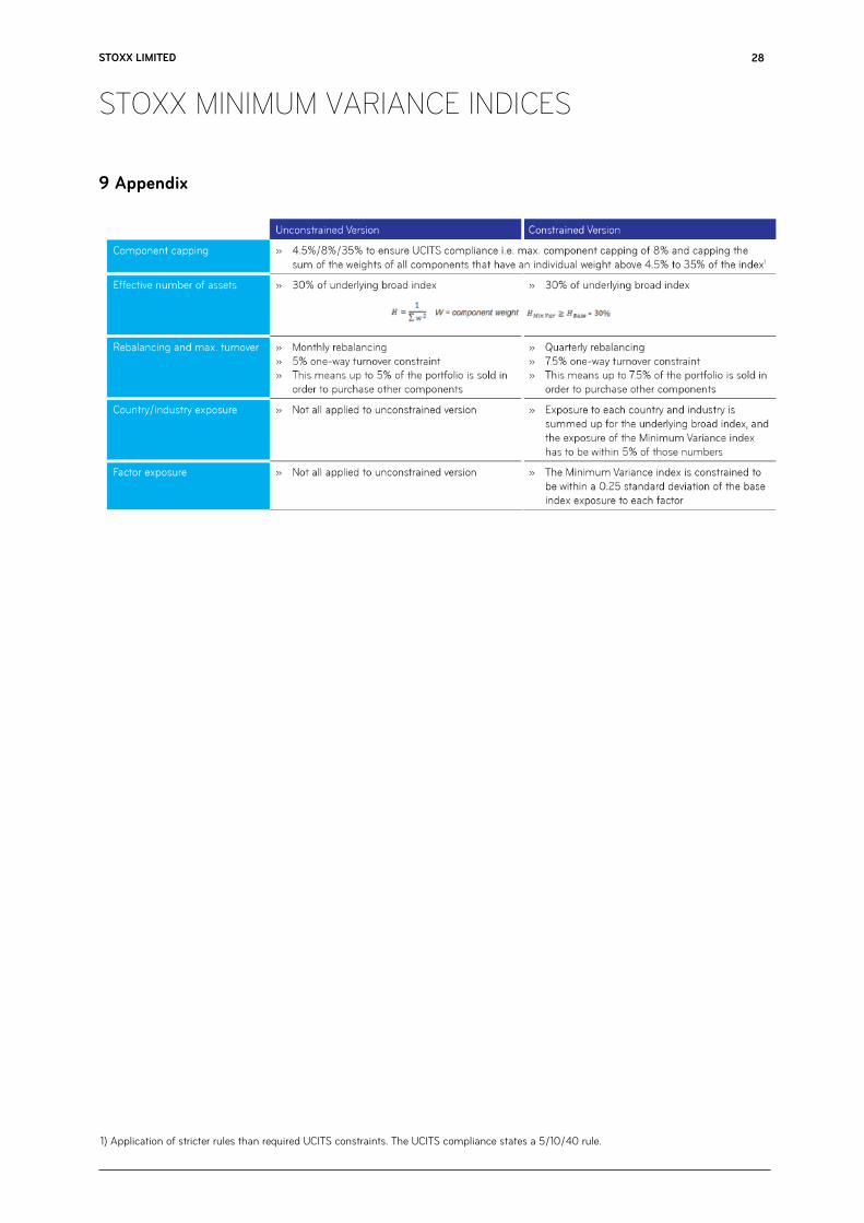
All indices comply with UCITS regulation at rebalancing; in fact the component capping applied is even stricter than UCITS requirements. Every component in the index is capped to have a maximum weight of 8%. All components with weight of at least 4.5% will not exceed 35% of the weight of the portfolio when combined. This 4.5/8/35 capping is a tougher application of the 5/10/40 standard so that compliance is very rarely breached and if there is ever a breach, it would take little trading to bring it back to compliance.

We then enforce that the minimum variance index has an effective number of assets of at least 30% of that of the base index. This is a neat (shall we say relevant) way of enforcing diversification without stating a specific number of assets (which an optimizer would just circumvent by applying insignificant

weights to additional components). This constraint is based on Hirsch-Herfindahl7 diversification, which is a well-accepted measure.

The Unconstrained index is rebalanced monthly and is allowed to have a turnover of 5% one-way (or 60% annual). The Constrained version rebalances quarterly with a 7.5% turnover (or 30% annual), in sync with the base index.

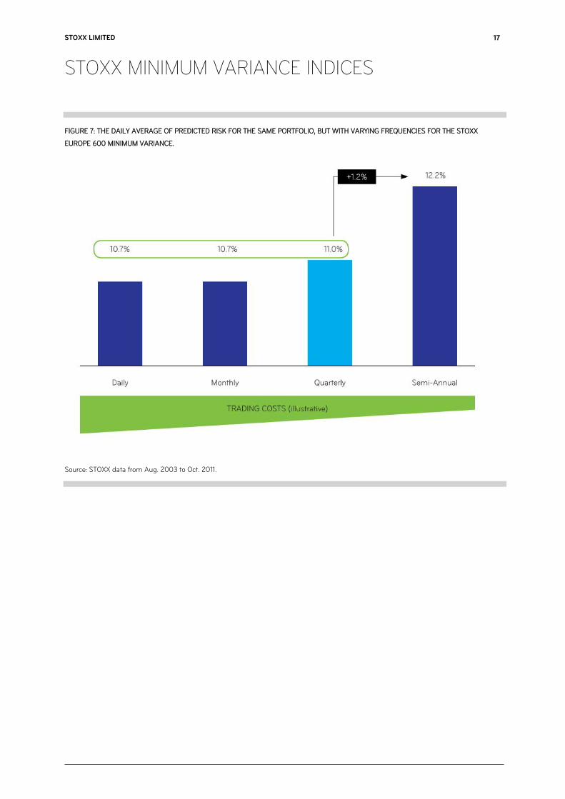
These are the only constraints applied on the Unconstrained version. In addition to these, we apply on the Constrained version relative exposure limits to countries, industries and risk factors. The Constrained minimum variance indices can only have the benchmark’s country and industry allocation +/- 5% and the style factors (all Axioma style factors except Size and Volatility) exposures have to be the same within a quarter standard deviation. Therefore, the Constrained minimum variance index takes on very similar risks as the benchmark, but to a lesser extent, and so the resulting portfolio is similar but reduced for risk (and increased for returns). Every day that the portfolio is not rebalanced, it will evolve in a non-optimal way as the weights change with market-price changes. In theory, any strategy should rebalance continuously, which is not feasible. Therefore there is a trade-off between transaction costs on one side and turnover and trading frequency on the other. There only seems to be a very significant risk increase when switching from quarterly to semi-annually and relatively minor impact switching from monthly to quarterly, as illustrated in Figure 5. Although semi-annual rebalancing is practical, the risk consequences of the choices have made STOXX choose smaller rebalancing frequencies. Furthermore it is important to remember that it is necessary to allow a certain amount of trading and turnover in order to make sure we do not lose too much of the concept’s value. On a long enough time scale without rebalancing, any portfolio becomes market-cap weighted.

7 "Herfindahl–Hirschman Index". USDOJ. Retrieved Dec. 31, 2013.

http://www.justice.gov/atr/public/guidelines/hhi.html

STOXX LIMITED


17

FIGURE 7: THE DAILY AVERAGE OF PREDICTED RISK FOR THE SAME PORTFOLIO, BUT WITH VARYING FREQUENCIES FOR THE STOXX

EUROPE 600 MINIMUM VARIANCE.

Source: STOXX data from Aug. 2003 to Oct. 2011.

STOXX LIMITED


18

6 Minimum variance performance

With all STOXX Minimum Variance Indices, we have witnessed consistent outperformance and extreme risk reduction across all regions and countries. Even in emerging markets, we have seen that there would be tremendous value in investing in minimum variance. We see a consistent picture across all markets, where the minimum variance Unconstrained index has the lowest risk of all, followed by the minimum variance index, which also significantly reduces risk. Performance-wise, the Unconstrained version is often the best performer, while both versions outperform the market systematically. Graphs and tables are attached in the appendix for all STOXX Minimum Variance indices and there are also some preliminary numbers on soon-to-come indices. An important point to note is that the performance of minimum variance is not fully defensive. In every market, minimum variance has outperformed every year the market has been down, but it has also outperformed on most positive years. As can be seen from Figure 8, minimum variance can outperform in bear and bull markets.

STOXX LIMITED


19

FIGURE 8: PERFORMANCE OF MINIMUM VARIANCE IN BULL AND BEAR MARKETS.

Source: STOXX daily data from Jan. 2, 2004 to Apr. 30, 2007 and Jun. 29, 2007 to Feb. 27, 2009 for EUR Net Return versions.

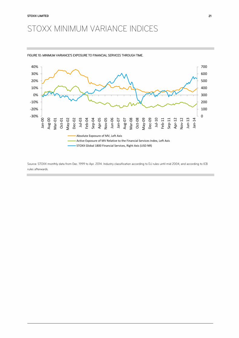
Minimum variance, seeking to minimize risk, has done very well in light of the global financial crisis. Looking at the allocation to financials before and during the crisis, we can understand the source of the outperformance. Indeed, minimum variance did not necessarily perceive individual financial stocks to become more risky, but the industry to become more correlated. Therefore the allocation to financial companies were minimized and the active allocation was negative years before the crash, as can be seen from Figures 9 and 10. In fact, looking at Figure 10, we see that the allocation to financials was at its absolute minimum when the financial index was at its peak (so at the exact time of the downfall). This means that minimum variance was poised protectively against the global financial crisis and could have served to point out that financial stocks were getting risky.

0

20

40

60

80

100

120

140

160

180

200

Jan-04 Jun-04 Nov-04 Apr-05 Sep-05 Feb-06 Jul-06 Dec-06

STOXX Global 1800

STOXX Global 1800 MinimumVariance

STOXX Global 1800 MinimumVariance Unconstrained

0

20

40

60

80

100

120

Jun-07 Sep-07 Dec-07 Mar-08 Jun-08 Sep-08 Dec-08

STOXX Global 1800

STOXX Global 1800 MinimumVariance

STOXX Global 1800 MinimumVariance Unconstrained

STOXX LIMITED


20

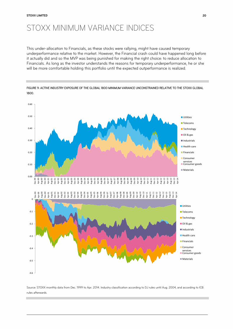
This under-allocation to Financials, as these stocks were rallying, might have caused temporary underperformance relative to the market. However, the Financial crash could have happened long before it actually did and so the MVP was being punished for making the right choice: to reduce allocation to Financials. As long as the investor understands the reasons for temporary underperformance, he or she will be more comfortable holding this portfolio until the expected outperformance is realized.

FIGURE 9: ACTIVE INDUSTRY EXPOSURE OF THE GLOBAL 1800 MINIMUM VARIANCE UNCONSTRAINED RELATIVE TO THE STOXX GLOBAL

1800.

Source: STOXX monthly data from Dec. 1999 to Apr. 2014. Industry classification according to DJ rules until Aug. 2004, and according to ICB

rules afterwards.

0.00

0.10

0.20

0.30

0.40

0.50

0.60

Dec

-99

Ap

r-00

Au

g-00

Dec

-00

Ap

r-01

Au

g-01

Dec

-01

Ap

r-02

Au

g-02

Dec

-02

Ap

r-03

Au

g-03

Dec

-03

Ap

r-04

Au

g-04

Dec

-04

Ap

r-05

Au

g-05

Dec

-05

Ap

r-06

Au

g-06

Dec

-06

Ap

r-07

Au

g-07

Dec

-07

Ap

r-08

Au

g-08

Dec

-08

Ap

r-09

Au

g-09

Dec

-09

Ap

r-10

Au

g-10

Dec

-10

Ap

r-11

Au

g-11

Dec

-11

Ap

r-12

Au

g-12

Dec

-12

Ap

r-13

Au

g-13

Dec

-13

Ap

r-14

Utilities

Telecoms

Technology

Oil & gas

Industrials

Health care

Financials

ConsumerservicesConsumer goods

Materials

-0.6

-0.5

-0.4

-0.3

-0.2

-0.1

0

Dec

-99

Ap

r-00

Au

g-00

Dec

-00

Ap

r-01

Au

g-01

Dec

-01

Ap

r-02

Au

g-02

Dec

-02

Ap

r-03

Au

g-03

Dec

-03

Ap

r-04

Au

g-04

Dec

-04

Ap

r-05

Au

g-05

Dec

-05

Ap

r-06

Au

g-06

Dec

-06

Ap

r-07

Au

g-07

Dec

-07

Ap

r-08

Au

g-08

Dec

-08

Ap

r-09

Au

g-09

Dec

-09

Ap

r-10

Au

g-10

Dec

-10

Ap

r-11

Au

g-11

Dec

-11

Ap

r-12

Au

g-12

Dec

-12

Ap

r-13

Au

g-13

Dec

-13

Ap

r-14

Utilities

Telecoms

Technology

Oil & gas

Industrials

Health care

Financials

ConsumerservicesConsumer goods

Materials

STOXX LIMITED


21

FIGURE 10: MINIMUM VARIANCE’S EXPOSURE TO FINANCIAL SERVICES THROUGH TIME.

Source: STOXX monthly data from Dec. 1999 to Apr. 2014. Industry classification according to DJ rules until mid 2004, and according to ICB

rules afterwards.

0

100

200

300

400

500

600

700

-30%

-20%

-10%

0%

10%

20%

30%

40%

Jan

-00

Au

g-0

0

Mar

-01

Oct

-01

May

-02

De

c-0

2

Jul-

03

Feb

-04

Sep

-04

Ap

r-0

5

No

v-0

5

Jun

-06

Jan

-07

Au

g-0

7

Mar

-08

Oct

-08

May

-09

De

c-0

9

Jul-

10

Feb

-11

Sep

-11

Ap

r-1

2

No

v-1

2

Jun

-13

Jan

-14

Absolute Exposure of MV, Left Axis

Active Exposure of MV Relative to the Financial Services Index, Left Axis

STOXX Global 1800 Financial Services, Right Axis (USD NR)

STOXX LIMITED


22

7 Putting the STOXX Minimum Variance indices to use

As we have observed, the MVP has become widely popular over the past few years, and it is not unreasonable to believe that risk awareness and aversion following the financial crisis have driven investors toward less risky investments. In the MVP, investors have found a product that not only lowers risk but also maintains and enhances returns over the long term, and crucially appears to be a strategy that is not easily arbitraged away. The analysis would suggest that the MVP is not just an investment to cover downside risk or for those that want to take an active ‘bet’ on the volatility of a region. But an MVP should be considered as part of an overall asset allocation for investors seeking to outperform the market or enter into better risk management. Many investors adopt a core-satellite approach to portfolio management whereby the core portfolio needs to have huge liquidity due to large amounts being managed, and satellites can have lower liquidity. In this framework, minimum variance provides an ideal investment strategy as a satellite. It benefits from a very low beta, low risk and high performance. This also means that it can be combined with a higher beta portfolio (e.g. small caps) to give an average beta in line with targets, while providing outperformance on each satellite. Looking at a practical example of this implementation in Europe, we can construct a portfolio with a beta of 1 using 60% core allocation to the market index (STOXX Europe 600) and 40% to two satellites (STOXX Europe 600 Minimum Variance Unconstrained and STOXX Europe Small 200) as shown in Figure 11.

STOXX LIMITED


23

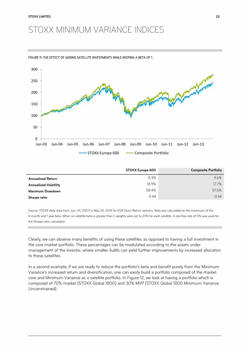
FIGURE 11: THE EFFECT OF ADDING SATELLITE INVESTMENTS WHILE KEEPING A BETA OF 1.

STOXX Europe 600 Composite Portfolio

Annualized Return 8.3% 9.6%

Annualized Volatility 18.9% 17.7%

Maximum Drawdown 58.4% 57.6%

Sharpe ratio 0.44 0.54

Source: STOXX daily data from Jun. 24, 2003 to May 30, 2014 for EUR Gross Return versions. Beta was calculated as the maximum of the

6 month and 1 year beta. When no satellite beta is greater than 1, weights were set to 20% for each satellite. A risk free rate of 0% was used for

the Sharpe ratio calculation.

Clearly, we can observe many benefits of using these satellites as opposed to having a full investment in the core market portfolio. These percentages can be modulated according to the assets under management of the investor, where smaller AuMs can yield further improvements by increased allocation to these satellites. In a second example, if we are ready to reduce the portfolio’s beta and benefit purely from the Minimum Variance’s increased return and diversification, one can easily build a portfolio composed of the market core and Minimum Variance as a satellite portfolio. In Figure 12, we look at having a portfolio which is composed of 70% market (STOXX Global 1800) and 30% MVP (STOXX Global 1800 Minimum Variance Unconstrained).

0

50

100

150

200

250

300

Jun-03 Jun-04 Jun-05 Jun-06 Jun-07 Jun-08 Jun-09 Jun-10 Jun-11 Jun-12 Jun-13

STOXX Europe 600 Composite Portfolio

STOXX LIMITED


24

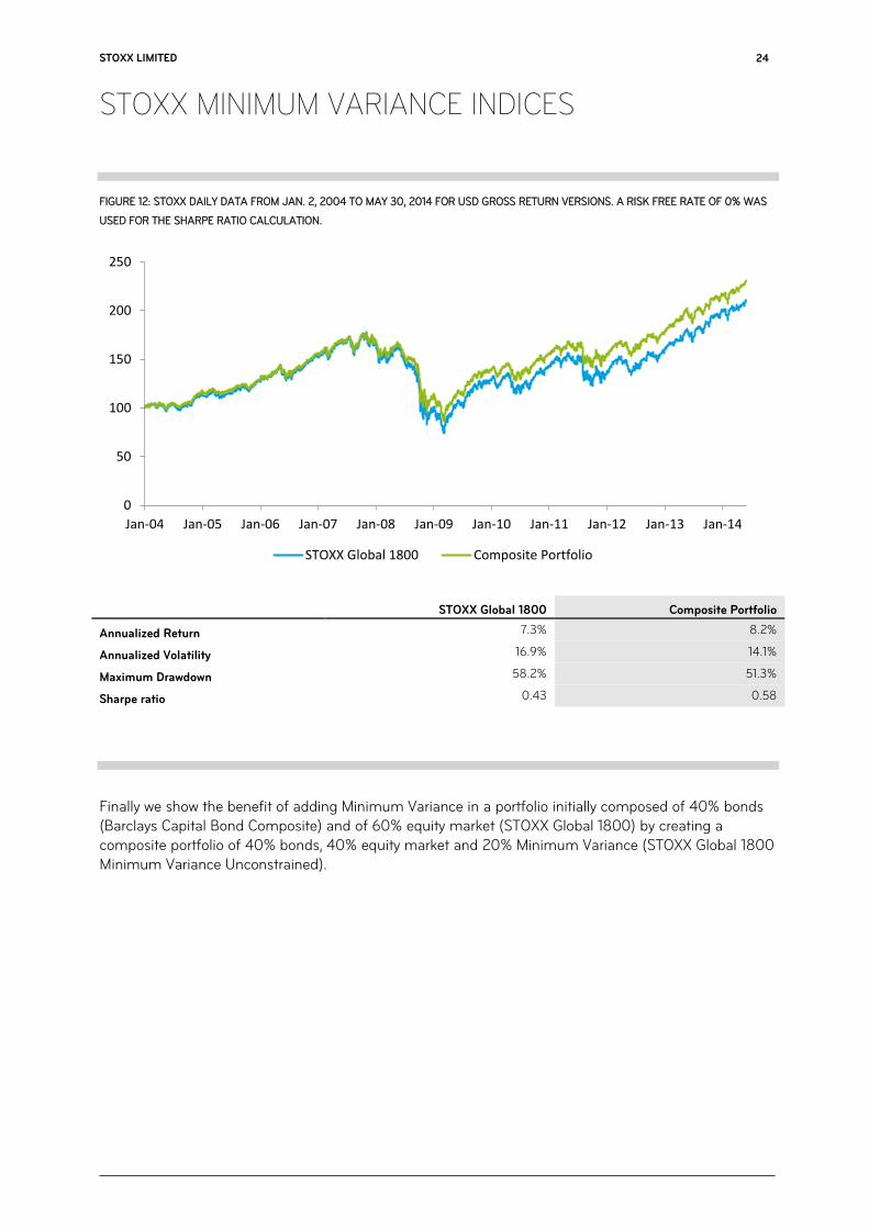
FIGURE 12: STOXX DAILY DATA FROM JAN. 2, 2004 TO MAY 30, 2014 FOR USD GROSS RETURN VERSIONS. A RISK FREE RATE OF 0% WAS

USED FOR THE SHARPE RATIO CALCULATION.

STOXX Global 1800 Composite Portfolio





Finally we show the benefit of adding Minimum Variance in a portfolio initially composed of 40% bonds (Barclays Capital Bond Composite) and of 60% equity market (STOXX Global 1800) by creating a composite portfolio of 40% bonds, 40% equity market and 20% Minimum Variance (STOXX Global 1800 Minimum Variance Unconstrained).

0

50

100

150

200

250

Jan-04 Jan-05 Jan-06 Jan-07 Jan-08 Jan-09 Jan-10 Jan-11 Jan-12 Jan-13 Jan-14

STOXX Global 1800 Composite Portfolio

STOXX LIMITED


25

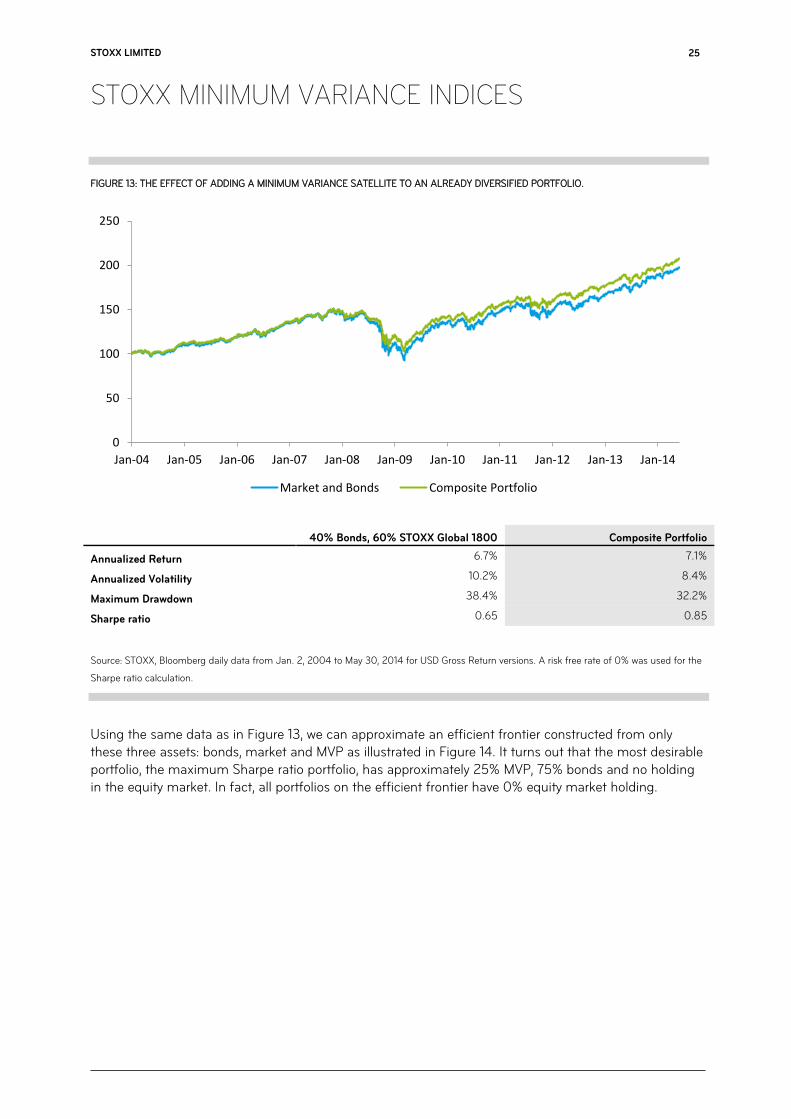
FIGURE 13: THE EFFECT OF ADDING A MINIMUM VARIANCE SATELLITE TO AN ALREADY DIVERSIFIED PORTFOLIO.

40% Bonds, 60% STOXX Global 1800 Composite Portfolio





Source: STOXX, Bloomberg daily data from Jan. 2, 2004 to May 30, 2014 for USD Gross Return versions. A risk free rate of 0% was used for the

Sharpe ratio calculation.

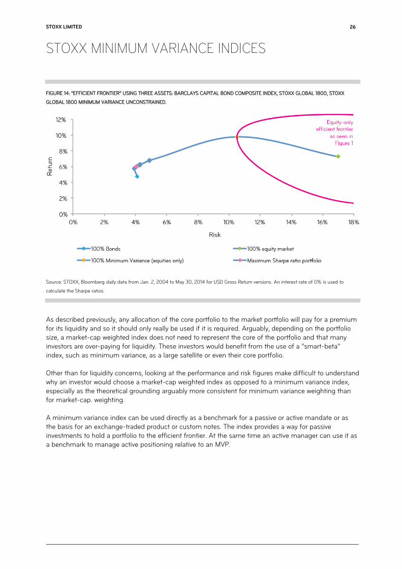
Using the same data as in Figure 13, we can approximate an efficient frontier constructed from only these three assets: bonds, market and MVP as illustrated in Figure 14. It turns out that the most desirable portfolio, the maximum Sharpe ratio portfolio, has approximately 25% MVP, 75% bonds and no holding in the equity market. In fact, all portfolios on the efficient frontier have 0% equity market holding.

0

50

100

150

200

250

Jan-04 Jan-05 Jan-06 Jan-07 Jan-08 Jan-09 Jan-10 Jan-11 Jan-12 Jan-13 Jan-14

Market and Bonds Composite Portfolio

STOXX LIMITED


26

FIGURE 14: “EFFICIENT FRONTIER” USING THREE ASSETS: BARCLAYS CAPITAL BOND COMPOSITE INDEX, STOXX GLOBAL 1800, STOXX

GLOBAL 1800 MINIMUM VARIANCE UNCONSTRAINED.

Source: STOXX, Bloomberg daily data from Jan. 2, 2004 to May 30, 2014 for USD Gross Return versions. An interest rate of 0% is used to

calculate the Sharpe ratios.

As described previously, any allocation of the core portfolio to the market portfolio will pay for a premium for its liquidity and so it should only really be used if it is required. Arguably, depending on the portfolio size, a market-cap weighted index does not need to represent the core of the portfolio and that many investors are over-paying for liquidity. These investors would benefit from the use of a “smart-beta” index, such as minimum variance, as a large satellite or even their core portfolio. Other than for liquidity concerns, looking at the performance and risk figures make difficult to understand why an investor would choose a market-cap weighted index as opposed to a minimum variance index, especially as the theoretical grounding arguably more consistent for minimum variance weighting than for market-cap. weighting. A minimum variance index can be used directly as a benchmark for a passive or active mandate or as the basis for an exchange-traded product or custom notes. The index provides a way for passive investments to hold a portfolio to the efficient frontier. At the same time an active manager can use it as a benchmark to manage active positioning relative to an MVP.

STOXX LIMITED


27

8 Conclusion

The minimum variance portfolio might be considered the “best of all worlds”: low risk, low drawdowns and long-term superior returns. As a strategy, minimum variance investing has clearly piqued the interest of a risk-aware, risk-averse investment community. The creation of minimum variance indices makes these strategies widely available to sponsors of financial instruments and as benchmarks for minimum variance strategies. However, not all minimum variance indices are created equally. To date, simple volatility weighting has proved more popular, but as we have seen such a strategy can lead to some significant issues, notably unintended concentration in sectors or risk factors. The STOXX Minimum Variance Indices put the choice into the hands of the investor. The Constrained version retains many of the characteristics of the underlying benchmark, whereas the Unconstrained version aims to generate a portfolio that most accurately represents the theoretical MVP with constraints only being applied to ensure that the portfolio remains investable.

STOXX LIMITED


28

9 Appendix

1) Application of stricter rules than required UCITS constraints. The UCITS compliance states a 5/10/40 rule.

NOTES

NOTES

NOTES

CONTACTS

Selnaustrasse 30 CH-8021 Zurich P +41 (0)58 399 5300 [email protected] www.stoxx.com Frankfurt: +49 (0)69 211 13243 Hong Kong: +852 6307 9316 London: +44 (0)20 7862 7680 Madrid: +34 (0)91 369 1229 New York: +1 212 669 6426

INNOVATIVE. GLOBAL. INDICES.

About STOXX STOXX Ltd. is a global index provider, currently calculating a global, comprehensive index family of over 6,000 strictly rules-based and transparent indices. Best known for the leading European equity indices EURO STOXX 50, STOXX Europe 50 and STOXX Europe 600, STOXX Ltd. maintains and calculates the STOXX Global index family which consists of total market, broad and blue-chip indices for the regions Americas, Europe, Asia/Pacific and sub-regions Latin America and BRIC (Brazil, Russia, India and China) as well as global markets. To provide market participants with optimal transparency, STOXX indices are classified into three categories. Regular “STOXX” indices include all standard, theme and strategy indices that are part of STOXX’s integrated index family and follow a strict rules-based methodology. The “iSTOXX” brand typically comprises less standardized index concepts that are not integrated in the STOXX Global index family, but are nevertheless strictly rules based. While indices that are branded “STOXX” and “iSTOXX” are developed by STOXX for a broad range of market participants, the “STOXX Customized” brand covers ind ices that are specifically developed for clients and do not carry the STOXX brand in the index name.

STOXX indices are licensed to more than 500 companies around the world as underlyings for Exchange Traded Funds (ETFs), futures and options, structured products and passively managed investment funds. Three of the top ETFs in Europe and 30% of all assets under management are based on STOXX indices. STOXX Ltd. holds Europe's number one and the world's number three position in the derivatives segment.

In addition, STOXX Ltd. is the marketing agent for the indices of Deutsche Boerse AG and SIX, amongst them the DAX and the SMI indices. STOXX Ltd. is part of Deutsche Boerse AG and SIX. www.stoxx.com

Documents

AUGUST, 2014 BUILDING MINIMUM VARIANCE PORTFOLIOS WITH · PDF fileINNOVATIVE. GLOBAL. INDICES. AUGUST, 2014 BUILDING MINIMUM VARIANCE PORTFOLIOS WITH LOW RISK, LOW DRAWDOWNS AND STRONG