Minimum Variance Portfolios - Northern Trust · Market turmoil has brought the topic of Minimum Variance Portfolios (MVP) ... the benefits of diversification and the concept of the

M I N I M U M V A R I A N C E P O R T F O L I O S

C h a l l e n g i n g T r a d i t i o n a l C o n c e p t s o f R i s k a n d R e w a r d

http://www.northerntrust.com/pws/jsp/display2.jsp?TYPE=landing&XML=pages/ntlanding/cis_europe&pageTimeout=600

Market turmoil has brought the topic of Minimum

Variance Portfolios (MVP) to the forefront. But when

we examined MVPs within a broad U.S. universe

and alongside the closely related Low Volatility

Portfolio (LVP) counterpart, we found ourselves

asking: are investors who employ these strategies

appropriately compensated for the relative risk

they assume?

With this paper, we work to answer this

question by studying the MVP and LVP strategies

and related academic literature; we then backtested

and compared the two strategies to a hypothetical

portfolio focused on the intersection of the highest-

quality companies offering a current dividend, the

Quality Dividend Focus (QDF) strategy. In the end,

we determined the QDF strategy is a compelling

option worth exploring.

2 of 16 | Minimum Variance Portfolio | northerntrust.com

A New Perspective on Risk and Return In our results, consistent with academic research, we found that although both genres of portfolio construction

techniques – minimum volatility and low volatility – deliver excess market return, their information ratios (IRs) are not

statistically significant. We found that both strategies force investors to assume considerable risk, relative to the market,

for which they are not compensated. Specifically, we found that these strategies have considerable relative downside

risk. Our backtest results are consistent with the academic literature on the subject, in that we found both portfolio

strategies have significant loading on the Value factor, as defined by the Fama-French-Carhart four-factor model. Finally,

we compared the backtested results of the MVP and LVP with those of a hypothetical low-volatility Quality Dividend

Focus (QDF) strategy. The low-volatility QDF backtest results showed that the strategy provides higher risk-adjusted

performance relative to the market, which is illustrated by a statistically significant IR. This indicates that, unlike the MVP

and LVP strategies, the low-volatility QDF strategy is compensated for its relative market risk.

Minimum Variance Portfolio (MVP)The concept of Modern Portfolio Theory i (MPT) has been the cornerstone of portfolio construction for academics and

practitioners alike since Harry Markowitz introduced it into finance in 1952. Every finance student learns the source of

portfolio volatility, the benefits of diversification and the concept of the efficient frontier. The portfolio of risky assets at

the starting point of the efficient frontier is known as the MVP.

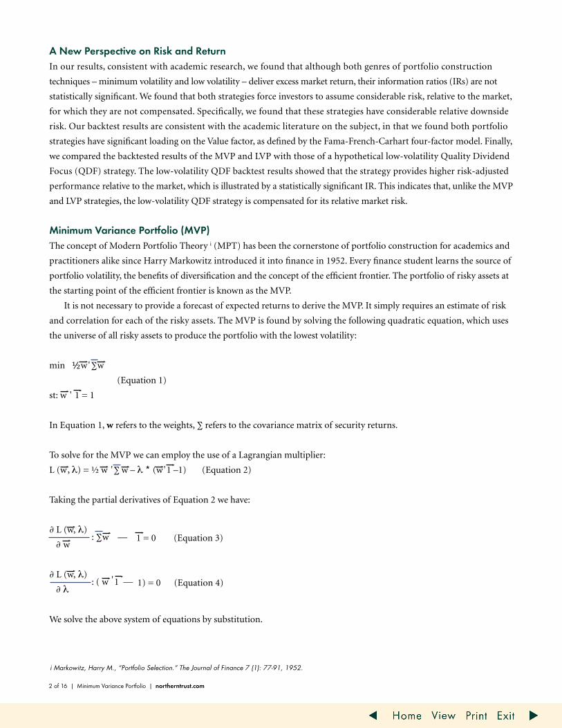
It is not necessary to provide a forecast of expected returns to derive the MVP. It simply requires an estimate of risk

and correlation for each of the risky assets. The MVP is found by solving the following quadratic equation, which uses

the universe of all risky assets to produce the portfolio with the lowest volatility:

min ½ w ' ∑ w

(Equation 1) st: w ' 1 = 1

In Equation 1, w refers to the weights, ∑ refers to the covariance matrix of security returns.

To solve for the MVP we can employ the use of a Lagrangian multiplier:

L (w , l) = ½ w ' ∑ w – l * (w ' 1 –1) (Equation 2) Taking the partial derivatives of Equation 2 we have:

∂ L (w, l) : ∑ w — 1 = 0 (Equation 3)

∂ w

∂ L (w, l) : ( w

' 1 — 1) = 0 (Equation 4)

∂ l

We solve the above system of equations by substitution.

i Markowitz, Harry M., “Portfolio Selection.” The Journal of Finance 7 (1): 77-91, 1952.


northerntrust.com | Minimum Variance Portfolio | 3 of 16

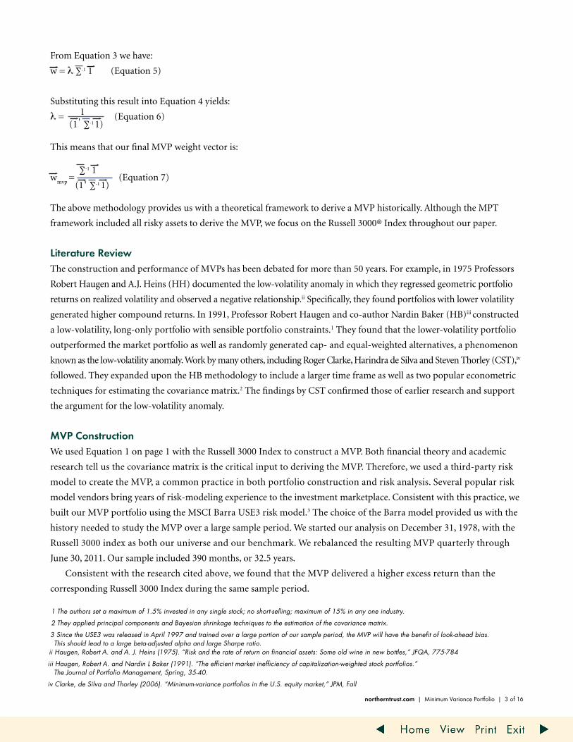
From Equation 3 we have:

w =l ∑-1 1 (Equation 5)

Substituting this result into Equation 4 yields:

l = 1 (Equation 6)

(1 ' ∑-1 1)

This means that our final MVP weight vector is:

wmvp

= ∑-1 1

(Equation 7) (1 ' ∑-1 1)

The above methodology provides us with a theoretical framework to derive a MVP historically. Although the MPT

framework included all risky assets to derive the MVP, we focus on the Russell 3000® Index throughout our paper.

Literature ReviewThe construction and performance of MVPs has been debated for more than 50 years. For example, in 1975 Professors

Robert Haugen and A.J. Heins (HH) documented the low-volatility anomaly in which they regressed geometric portfolio

returns on realized volatility and observed a negative relationship.ii Specifically, they found portfolios with lower volatility

generated higher compound returns. In 1991, Professor Robert Haugen and co-author Nardin Baker (HB)iii constructed

a low-volatility, long-only portfolio with sensible portfolio constraints.1 They found that the lower-volatility portfolio

outperformed the market portfolio as well as randomly generated cap- and equal-weighted alternatives, a phenomenon

known as the low-volatility anomaly. Work by many others, including Roger Clarke, Harindra de Silva and Steven Thorley (CST),iv

followed. They expanded upon the HB methodology to include a larger time frame as well as two popular econometric

techniques for estimating the covariance matrix.2 The findings by CST confirmed those of earlier research and support

the argument for the low-volatility anomaly.

MVP ConstructionWe used Equation 1 on page 1 with the Russell 3000 Index to construct a MVP. Both financial theory and academic

research tell us the covariance matrix is the critical input to deriving the MVP. Therefore, we used a third-party risk

model to create the MVP, a common practice in both portfolio construction and risk analysis. Several popular risk

model vendors bring years of risk-modeling experience to the investment marketplace. Consistent with this practice, we

built our MVP portfolio using the MSCI Barra USE3 risk model.3 The choice of the Barra model provided us with the

history needed to study the MVP over a large sample period. We started our analysis on December 31, 1978, with the

Russell 3000 index as both our universe and our benchmark. We rebalanced the resulting MVP quarterly through

June 30, 2011. Our sample included 390 months, or 32.5 years.

Consistent with the research cited above, we found that the MVP delivered a higher excess return than the

corresponding Russell 3000 Index during the same sample period.

1 The authors set a maximum of 1.5% invested in any single stock; no short-selling; maximum of 15% in any one industry.

2 They applied principal components and Bayesian shrinkage techniques to the estimation of the covariance matrix. 3 Since the USE3 was released in April 1997 and trained over a large portion of our sample period, the MVP will have the benefit of look-ahead bias. This should lead to a large beta-adjusted alpha and large Sharpe ratio.

ii Haugen, Robert A. and A. J. Heins (1975). “Risk and the rate of return on financial assets: Some old wine in new bottles,” JFQA, 775-784

iii Haugen, Robert A. and Nardin L Baker (1991). “The efficient market inefficiency of capitalization-weighted stock portfolios.” The Journal of Portfolio Management, Spring, 35-40.

iv Clarke, de Silva and Thorley (2006). “Minimum-variance portfolios in the U.S. equity market,” JPM, Fall



-1000%

0%

1000%

2000%

3000%

4000%

5000%

6000%

7000%

8000%

9000%

RUSSELL 3000 RELATIVEMVP

CU

MU

LATI

VE R

ETU

RN

12/3

1/78

12/3

1/79

12/3

1/80

12/3

1/81

12/3

1/82

12/3

1/83

12/3

1/84

12/3

1/85

6/30

/11

12/3

1/86

12/3

1/87

12/3

1/88

12/3

1/89

12/3

1/90

12/3

1/91

12/3

1/92

12/3

1/93

12/3

1/94

12/3

1/95

12/3

1/96

12/3

1/97

12/3

1/98

12/3

1/99

12/3

1/01

12/3

1/02

12/3

1/03

12/3

1/04

12/3

1/05

12/3

1/06

12/3

1/07

12/3

1/08

12/3

1/09

12/3

1/10

12/3

1/00

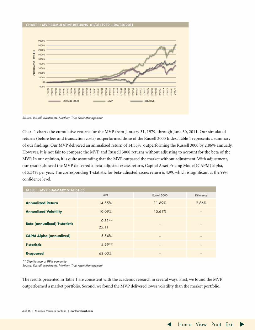
ChART 1: MVP CUMULATIVE RETURNS 01/31/1979 – 06/30/2011

Source: Russell Investments, Northern Trust Asset Management

Chart 1 charts the cumulative returns for the MVP from January 31, 1979, through June 30, 2011. Our simulated

returns (before fees and transaction costs) outperformed those of the Russell 3000 Index. Table 1 represents a summary

of our findings. Our MVP delivered an annualized return of 14.55%, outperforming the Russell 3000 by 2.86% annually.

However, it is not fair to compare the MVP and Russell 3000 returns without adjusting to account for the beta of the

MVP. In our opinion, it is quite astounding that the MVP outpaced the market without adjustment. With adjustment,

our results showed the MVP delivered a beta-adjusted excess return, Capital Asset Pricing Model (CAPM) alpha,

of 5.54% per year. The corresponding T-statistic for beta-adjusted excess return is 4.99, which is significant at the 99%

confidence level.

** Significance at 99th percentile Source: Russell Investments, Northern Trust Asset Management

The results presented in Table 1 are consistent with the academic research in several ways. First, we found the MVP

outperformed a market portfolio. Second, we found the MVP delivered lower volatility than the market portfolio.

TAbLE 1: MVP SUMMARy STATISTICSMVP Russell 3000 Difference

Annualized Return 14.55% 11.69% 2.86%

Annualized Volatility 10.09% 15.61% –

Beta (annualized) T-statistic0.51**

25.11– –

CAPM Alpha (annualized) 5.54% – –

T-statistic 4.99** – –

R-squared 63.00% – –


However, a closer look at our MVP showed some concerning trends. First, the portfolio can become fairly concentrated.

It is not uncommon to have at least 20% of the portfolio invested in a single name at any point. Having such a large

position in any one name increases the impact of an idiosyncratic shock to the portfolio out-of-sample, makes trading

more problematic as liquidity becomes an issue, and can lead to higher turnover and transaction costs.

Second, we found the portfolio had large sector biases. The MVP took on large over-weights to utilities and

telecommunication services as well as large under-weights to information technology and consumer discretionary.

Chart 2 displays a time series of sector weights for the MVP. During the late 1980s, nearly 70% of the portfolio was

invested in utilities. Currently, close to 50% of the portfolio is invested in consumer staples.

Source: Standard & Poor’s, Northern Trust Asset Management

Third, we found the MVP experienced high average annual turnover of approximately 130%. This far exceeded the rate

for the broader market as represented by the Russell 3000, which had an average annual turnover of less than 5% during

the past 10 years. Finally, we found the MVP failed to deliver a statistically significant Information Ratio (IR)4 to the

Russell 3000 Index.

Although the results presented in Table 1 appear to be impressive, the relative returns are not statistically significant.

Table 2 displays a summary of relative return and relative risk statistics. We found the realized tracking error, relative to

the Russell 3000, was 9.78% during the sample period. Although the MVP outperformed by 2.86%, the IR was only 0.29

with a T-statistic of 1.64 (not statistically significant at the 95th percentile).

4 IR =

(annual Portfolio return – annual Russell 3000 return) (annual standard deviation of excess returns)


0%

10%

20%

30%

40%

50%

60%

70%

80%

90%

100%

UTILITIES TELECOMMUNICATION SERVICES MATERIALS INFORMATION TECHNOLOGY

INDUSTRIALS HEALTH CARE FINANCIALS ENERGY CONSUMER STAPLES

CONSUMER DISCRETIONARY

SEC

TOR

WEI

GH

T

12/3

1/78

12/3

1/79

12/3

1/80

12/3

1/81

12/3

1/82

12/3

1/83

12/3

1/84

12/3

1/85

6/30

/11

12/3

1/86

12/3

1/87

12/3

1/88

12/3

1/89

12/3

1/90

12/3

1/91

12/3

1/92

12/3

1/93

12/3

1/94

12/3

1/95

12/3

1/96

12/3

1/97

12/3

1/98

12/3

1/99

12/3

1/01

12/3

1/02

12/3

1/03

12/3

1/04

12/3

1/05

12/3

1/06

12/3

1/07

12/3

1/08

12/3

1/09

12/3

1/10

12/3

1/00

ChART 2: PORTFOLIO SECTOR WEIghTS 01/31/1979 – 06/30/2011



* Not statistically significant at the 95th percentile

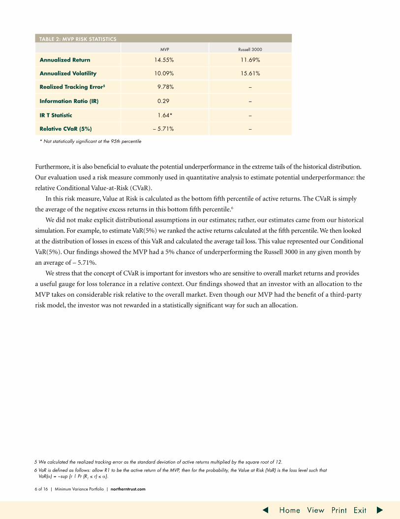
Furthermore, it is also beneficial to evaluate the potential underperformance in the extreme tails of the historical distribution.

Our evaluation used a risk measure commonly used in quantitative analysis to estimate potential underperformance: the

relative Conditional Value-at-Risk (CVaR).

In this risk measure, Value at Risk is calculated as the bottom fifth percentile of active returns. The CVaR is simply

the average of the negative excess returns in this bottom fifth percentile.6

We did not make explicit distributional assumptions in our estimates; rather, our estimates came from our historical

simulation. For example, to estimate VaR(5%) we ranked the active returns calculated at the fifth percentile. We then looked

at the distribution of losses in excess of this VaR and calculated the average tail loss. This value represented our Conditional

VaR(5%). Our findings showed the MVP had a 5% chance of underperforming the Russell 3000 in any given month by

an average of – 5.71%.

We stress that the concept of CVaR is important for investors who are sensitive to overall market returns and provides

a useful gauge for loss tolerance in a relative context. Our findings showed that an investor with an allocation to the

MVP takes on considerable risk relative to the overall market. Even though our MVP had the benefit of a third-party

risk model, the investor was not rewarded in a statistically significant way for such an allocation.

TAbLE 2: MVP RISk STATISTICS

MVP Russell 3000

Annualized Return 14.55% 11.69%

Annualized Volatility 10.09% 15.61%

Realized Tracking Error5 9.78% –

Information Ratio (IR) 0.29 –

IR T Statistic 1.64* –

Relative CVaR (5%) – 5.71% –

5 We calculated the realized tracking error as the standard deviation of active returns multiplied by the square root of 12.

6 VaR is defined as follows: allow R1 to be the active return of the MVP, then for the probability, the Value at Risk (VaR) is the loss level such that VaR(α) = −sup {r | Pr (R1 ≤ r) ≤ α}.


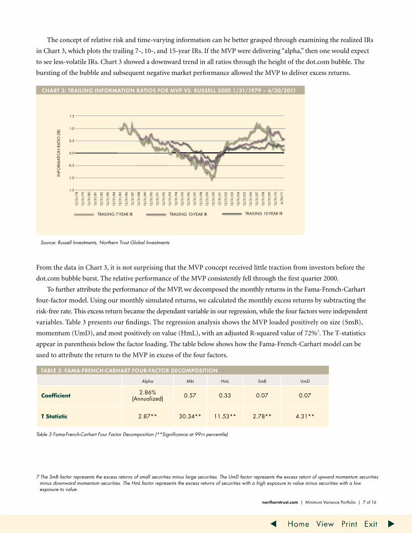
The concept of relative risk and time-varying information can be better grasped through examining the realized IRs

in Chart 3, which plots the trailing 7-, 10-, and 15-year IRs. If the MVP were delivering “alpha,” then one would expect

to see less-volatile IRs. Chart 3 showed a downward trend in all ratios through the height of the dot.com bubble. The

bursting of the bubble and subsequent negative market performance allowed the MVP to deliver excess returns.

Source: Russell Investments, Northern Trust Global Investments

From the data in Chart 3, it is not surprising that the MVP concept received little traction from investors before the

dot.com bubble burst. The relative performance of the MVP consistently fell through the first quarter 2000.

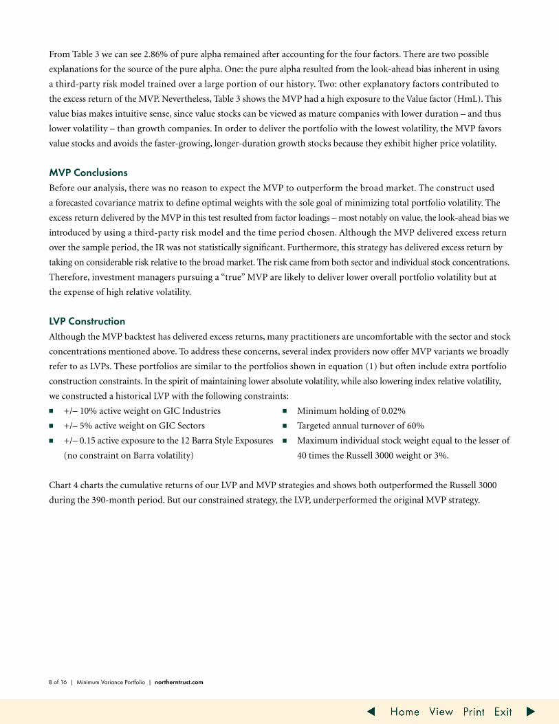
To further attribute the performance of the MVP, we decomposed the monthly returns in the Fama-French-Carhart

four-factor model. Using our monthly simulated returns, we calculated the monthly excess returns by subtracting the

risk-free rate. This excess return became the dependant variable in our regression, while the four factors were independent

variables. Table 3 presents our findings. The regression analysis shows the MVP loaded positively on size (SmB),

momentum (UmD), and most positively on value (HmL), with an adjusted R-squared value of 72%7. The T-statistics

appear in parenthesis below the factor loading. The table below shows how the Fama-French-Carhart model can be

used to attribute the return to the MVP in excess of the four factors.


-1.5

-1.0

-0.5

0.0

0.5

1.0

1.5

TRAILING 7-YEAR IR TRAILING 15-YEAR IRTRAILING 10-YEAR IR

INFO

RMA

TIO

N R

ATI

O (I

R)

12/3

1/78

12/3

1/79

12/3

1/80

12/3

1/81

12/3

1/82

12/3

1/83

12/3

1/84

12/3

1/85

6/30

/11

12/3

1/86

12/3

1/87

12/3

1/88

12/3

1/89

12/3

1/90

12/3

1/91

12/3

1/92

12/3

1/93

12/3

1/94

12/3

1/95

12/3

1/96

12/3

1/97

12/3

1/98

12/3

1/99

12/3

1/01

12/3

1/02

12/3

1/03

12/3

1/04

12/3

1/05

12/3

1/06

12/3

1/07

12/3

1/08

12/3

1/09

12/3

1/10

12/3

1/00

ChART 3: TRAILINg INFORMATION RATIOS FOR MVP VS. RUSSELL 3000 1/31/1979 – 6/30/2011

TAbLE 3: FAMA-FRENCh-CARhART FOUR-FACTOR dECOMPOSITION

Alpha Mkt HmL SmB UmD

Coefficient 2.86% (Annualized) 0.57 0.33 0.07 0.07

T Statistic 2.87** 30.34** 11.53** 2.78** 4.31**

Table 3 Fama-French-Carhart Four Factor Decomposition (**Significance at 99th percentile)

7 The SmB factor represents the excess returns of small securities minus large securities. The UmD factor represents the excess return of upward momentum securities minus downward momentum securities. The HmL factor represents the excess returns of securities with a high exposure to value minus securities with a low exposure to value.



From Table 3 we can see 2.86% of pure alpha remained after accounting for the four factors. There are two possible

explanations for the source of the pure alpha. One: the pure alpha resulted from the look-ahead bias inherent in using

a third-party risk model trained over a large portion of our history. Two: other explanatory factors contributed to

the excess return of the MVP. Nevertheless, Table 3 shows the MVP had a high exposure to the Value factor (HmL). This

value bias makes intuitive sense, since value stocks can be viewed as mature companies with lower duration – and thus

lower volatility – than growth companies. In order to deliver the portfolio with the lowest volatility, the MVP favors

value stocks and avoids the faster-growing, longer-duration growth stocks because they exhibit higher price volatility.

MVP ConclusionsBefore our analysis, there was no reason to expect the MVP to outperform the broad market. The construct used

a forecasted covariance matrix to define optimal weights with the sole goal of minimizing total portfolio volatility. The

excess return delivered by the MVP in this test resulted from factor loadings – most notably on value, the look-ahead bias we

introduced by using a third-party risk model and the time period chosen. Although the MVP delivered excess return

over the sample period, the IR was not statistically significant. Furthermore, this strategy has delivered excess return by

taking on considerable risk relative to the broad market. The risk came from both sector and individual stock concentrations.

Therefore, investment managers pursuing a “true” MVP are likely to deliver lower overall portfolio volatility but at

the expense of high relative volatility.

LVP ConstructionAlthough the MVP backtest has delivered excess returns, many practitioners are uncomfortable with the sector and stock

concentrations mentioned above. To address these concerns, several index providers now offer MVP variants we broadly

refer to as LVPs. These portfolios are similar to the portfolios shown in equation (1) but often include extra portfolio

construction constraints. In the spirit of maintaining lower absolute volatility, while also lowering index relative volatility,

we constructed a historical LVP with the following constraints:

■■ +/– 10% active weight on GIC Industries

■■ +/– 5% active weight on GIC Sectors

■■ +/– 0.15 active exposure to the 12 Barra Style Exposures

(no constraint on Barra volatility)

■■ Minimum holding of 0.02%

■■ Targeted annual turnover of 60%

■■ Maximum individual stock weight equal to the lesser of

40 times the Russell 3000 weight or 3%.

Chart 4 charts the cumulative returns of our LVP and MVP strategies and shows both outperformed the Russell 3000

during the 390-month period. But our constrained strategy, the LVP, underperformed the original MVP strategy.




**Significant at the 99% level

Table 4 displays the relative return statistics of both strategies discussed thus far. The excess return of the LVP strategy is

considerably lower than the MVP; however, the LVP has a similar IR and significantly less realized tracking error to the

Russell 3000 index. The LVP does not suffer from excessive concentration, turnover or unwanted portfolio exposures

due to the portfolio constraints outlined at the beginning of this section. The reduction in the relative risk also reduced

the CVaR by more than 2%. With the LVP strategy, there is now a 5% chance that the portfolio will underperform the

market by an average of – 3.53%, a considerable improvement over the downside risk of – 5.71% inherent in the

MVP strategy.

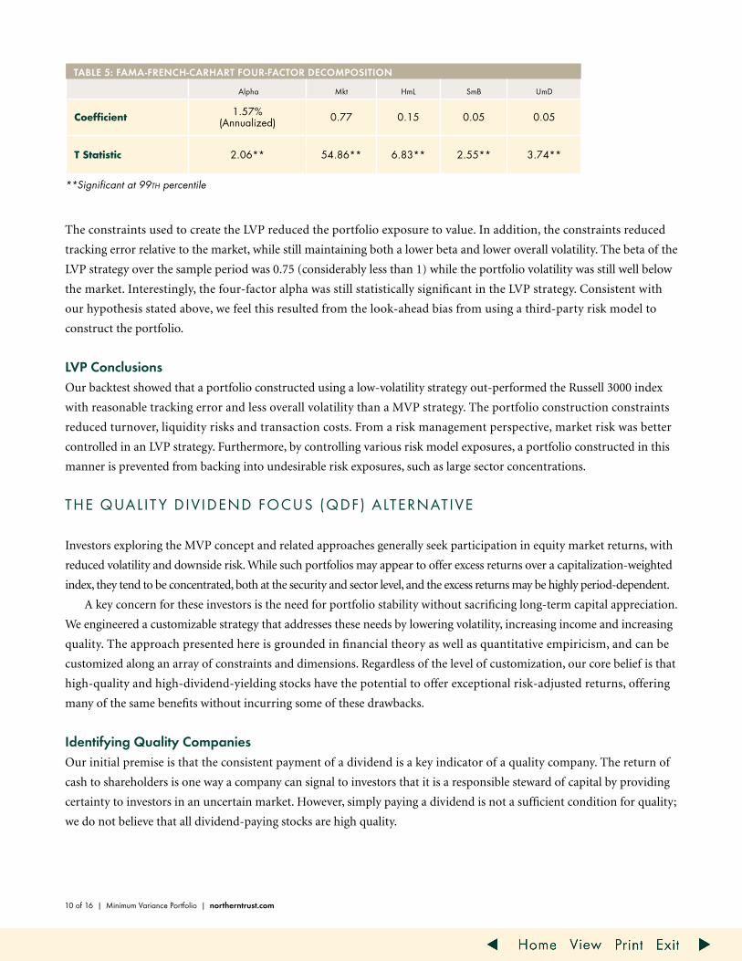
Table 5 displays the Fama-French-Carhart four-factor decomposition. Similar to the MVP analysis, we find the LVP

loads positively on all factors and most heavily on the value factor. The adjusted R-squared for this analysis is 90%.

TAbLE 4: MVP, LVP RELATIVE RETURN & RISk SUMMARy

LVP MVP Russell 3000

Annualized Return 13.30% 14.55% 11.69%

Annualized Volatility 12.61% 10.09% 15.61%

Excess Return 1.61% 2.86% –

Realized Tracking Error 5.66% 9.78% –

IR 0.28 0.29 –

IR T Statistic 1.57 1.63 –

Relative CVaR (5%) – 3.53% – 5.71% –

0

1000%

2000%

3000%

4000%

5000%

6000%

7000%

8000%

9000%

000

LVP RUSSELL 3000MVP

CU

MU

LATI

VE R

ETU

RN

12/3

1/78

12/3

1/79

12/3

1/80

12/3

1/81

12/3

1/82

12/3

1/83

12/3

1/84

12/3

1/85

6/30

/11

12/3

1/86

12/3

1/87

12/3

1/88

12/3

1/89

12/3

1/90

12/3

1/91

12/3

1/92

12/3

1/93

12/3

1/94

12/3

1/95

12/3

1/96

12/3

1/97

12/3

1/98

12/3

1/99

12/3

1/01

12/3

1/02

12/3

1/03

12/3

1/04

12/3

1/05

12/3

1/06

12/3

1/07

12/3

1/08

12/3

1/09

12/3

1/10

12/3

1/00

ChART 4: CUMULATIVE RETURNS 01/31/1979 – 06/30/2011



The constraints used to create the LVP reduced the portfolio exposure to value. In addition, the constraints reduced

tracking error relative to the market, while still maintaining both a lower beta and lower overall volatility. The beta of the

LVP strategy over the sample period was 0.75 (considerably less than 1) while the portfolio volatility was still well below

the market. Interestingly, the four-factor alpha was still statistically significant in the LVP strategy. Consistent with

our hypothesis stated above, we feel this resulted from the look-ahead bias from using a third-party risk model to

construct the portfolio.

LVP ConclusionsOur backtest showed that a portfolio constructed using a low-volatility strategy out-performed the Russell 3000 index

with reasonable tracking error and less overall volatility than a MVP strategy. The portfolio construction constraints

reduced turnover, liquidity risks and transaction costs. From a risk management perspective, market risk was better

controlled in an LVP strategy. Furthermore, by controlling various risk model exposures, a portfolio constructed in this

manner is prevented from backing into undesirable risk exposures, such as large sector concentrations.

THE QUALIT y DIVIDEND FoCUS (QDF) ALTERNATIVE

Investors exploring the MVP concept and related approaches generally seek participation in equity market returns, with

reduced volatility and downside risk. While such portfolios may appear to offer excess returns over a capitalization-weighted

index, they tend to be concentrated, both at the security and sector level, and the excess returns may be highly period-dependent.

A key concern for these investors is the need for portfolio stability without sacrificing long-term capital appreciation.

We engineered a customizable strategy that addresses these needs by lowering volatility, increasing income and increasing

quality. The approach presented here is grounded in financial theory as well as quantitative empiricism, and can be

customized along an array of constraints and dimensions. Regardless of the level of customization, our core belief is that

high-quality and high-dividend-yielding stocks have the potential to offer exceptional risk-adjusted returns, offering

many of the same benefits without incurring some of these drawbacks.

Identifying Quality CompaniesOur initial premise is that the consistent payment of a dividend is a key indicator of a quality company. The return of

cash to shareholders is one way a company can signal to investors that it is a responsible steward of capital by providing

certainty to investors in an uncertain market. However, simply paying a dividend is not a sufficient condition for quality;

we do not believe that all dividend-paying stocks are high quality.

TAbLE 5: FAMA-FRENCh-CARhART FOUR-FACTOR dECOMPOSITION

Alpha Mkt HmL SmB UmD

Coefficient 1.57% (Annualized) 0.77 0.15 0.05 0.05

T Statistic 2.06** 54.86** 6.83** 2.55** 3.74**

**Significant at 99th percentile



Among dividend-paying stocks, we further delineate quality by using a quantitative model that qualifies a company’s

ability to sustain its indicated dividend. Our Quality Score (QS) methodology assigns each dividend-paying firm a

quality rank based upon firm profitability, management efficiency and cash levels.

We measure the profitability of each firm to assess its competitive advantage. Our hypothesis is that a firm with a

competitive advantage relative to its peer group can deliver excess return to enterprise holders through higher profitability,

greater cash flows and thus increased dividends. One important factor in the analysis is the firm’s return on equity

(ROE), which typically negatively correlates with the stock’s dividend yield. Although one may argue that a firm with

a high ROE should retain earnings and reinvest for subsequent growth, our research shows firms with high ROEs,

dividend payments and moderate investment are more likely to sustain and grow their dividends over time. Thus, they

display attributes of a quality company.

Management efficiency is another important factor in our analysis. Our hypothesis is that a quality firm has prudent

investment management and will act on the behalf of enterprise holders through judicious use of capital. Our research

shows that firms with overly aggressive management may over-deploy capital. By overextending capital and entering

into excessive commitments, these firms are less likely to deliver positive, incremental return to enterprise holders. Since

capital expenditures can be difficult to cancel once started, firms that over-expand often fail to have the flexibility to

strategically maneuver in volatile markets. For example, many homebuilders over extrapolated the housing boom into

perpetuity, leading to an over-deployment of capital and increase in financial leverage. As the economy and housing

market began to weaken, firms that over-aggressively deployed capital found it difficult to sustain free cash flow. With an

economic shock to their top-line growth and increased capital cost structure, margins quickly turned negative, and these

firms struggled to meet their financial obligations. Another signal of overly aggressive management is a firm’s use of

external financing. History has taught us that companies can over-extrapolate the synergies and cost advantages associated

with expansions and acquisitions. The companies that are very aggressive in this dimension often find it difficult to

sustain dividend payments when their margins are under pressure. Thus, a quality company is one that uses leverage in

a prudent and conservative manner.

The third factor we use to measure quality is the level of cash needed to sustain the indicated dividend. Our hypothesis

is that quality companies have more than enough cash on hand to meet their debt obligations and day-to-day liquidity

needs, as well as sustain their indicated dividends. Also, our research shows that companies that pay dividends and have

a healthy amount of cash on their balance sheets tend to increase their dividends in the subsequent year.

Thus, even though investing in high-dividend-yielding stocks can add value, the notion of quality also forms a

cornerstone of the QDF methodology. We believe – and our research supports – that engineering a portfolio that tilts

toward high-quality and high-dividend-yielding stocks can be key to delivering positive risk-adjusted returns.




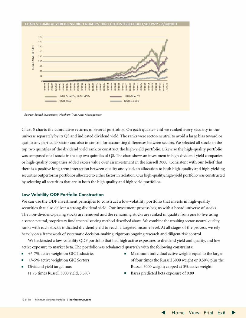
Chart 5 charts the cumulative returns of several portfolios. On each quarter-end we ranked every security in our

universe separately by its QS and indicated dividend yield. The ranks were sector-neutral to avoid a large bias toward or

against any particular sector and also to control for accounting differences between sectors. We selected all stocks in the

top two quintiles of the dividend yield rank to construct the high-yield portfolio. Likewise the high-quality portfolio

was composed of all stocks in the top two quintiles of QS. The chart shows an investment in high-dividend-yield companies

or high-quality companies added excess value over an investment in the Russell 3000. Consistent with our belief that

there is a positive long-term interaction between quality and yield, an allocation to both high-quality and high-yielding

securities outperforms portfolios allocated to either factor in isolation. Our high-quality/high-yield portfolio was constructed

by selecting all securities that are in both the high quality and high yield portfolios.

Low Volatility QdF Portfolio ConstructionWe can use the QDF investment principles to construct a low-volatility portfolio that invests in high-quality

securities that also deliver a strong dividend yield. Our investment process begins with a broad universe of stocks.

The non-dividend-paying stocks are removed and the remaining stocks are ranked in quality from one to five using

a sector-neutral, proprietary fundamental scoring method described above. We combine the resulting sector-neutral quality

ranks with each stock’s indicated dividend yield to reach a targeted income level. At all stages of the process, we rely

heavily on a framework of systematic decision-making, rigorous ongoing research and diligent risk control.

We backtested a low-volatility QDF portfolio that had high active exposures to dividend yield and quality, and low

active exposure to market beta. The portfolio was rebalanced quarterly with the following constraints:

■■ +/–7% active weight on GIC Industries

■■ +/–5% active weight on GIC Sectors

■■ Dividend yield target max

(1.75 times Russell 3000 yield, 3.5%)

■■ Maximum individual active weights equal to the larger

of four times the Russell 3000 weight or 0.50% plus the

Russell 3000 weight; capped at 3% active weight.

■■ Barra predicted beta exposure of 0.80

ChART 5: CUMULATIVE RETURNS: hIgh QUALITy/ hIgh yIELd INTERSECTION 1/31/1979 – 6/30/2011

0

50

100

150

200

250

300

350

400

450

0

0

0

0

0

0

0

0

0

0

0

0

0

0

0

0

0

0

0

0

HIGH QUALITY/ HIGH YIELD HIGH QUALITY

CU

MU

LATI

VE R

ETU

RN

HIGH YIELD RUSSELL 3000

12/3

1/78

12/3

1/79

12/3

1/80

12/3

1/81

12/3

1/82

12/3

1/83

12/3

1/84

12/3

1/85

6/30

/11

12/3

1/86

12/3

1/87

12/3

1/88

12/3

1/89

12/3

1/90

12/3

1/91

12/3

1/92

12/3

1/93

12/3

1/94

12/3

1/95

12/3

1/96

12/3

1/97

12/3

1/98

12/3

1/99

12/3

1/01

12/3

1/02

12/3

1/03

12/3

1/04

12/3

1/05

12/3

1/06

12/3

1/07

12/3

1/08

12/3

1/09

12/3

1/10

12/3

1/00




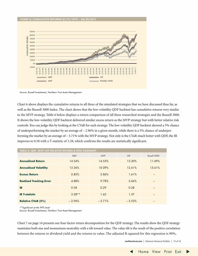
Chart 6 above displays the cumulative returns to all three of the simulated strategies that we have discussed thus far, as

well as the Russell 3000 Index. The chart shows that the low-volatility QDF backtest has cumulative returns very similar

to the MVP strategy. Table 6 below displays a return comparison of all three researched strategies and the Russell 3000.

It shows the low-volatility QDF backtest delivered similar excess return as the MVP strategy but with better relative risk

controls. You can judge this by looking at the CVaR for each strategy. The low-volatility QDF backtest showed a 5% chance

of underperforming the market by an average of – 2.96% in a given month, while there is a 5% chance of underper-

forming the market by an average of – 5.71% with the MVP strategy. Not only is the CVaR much better with QDF, the IR

improves to 0.58 with a T-statistic of 3.28, which confirms the results are statistically significant.

**Significant at the 99% level Source: Russell Investments, Northern Trust Asset Management

Chart 7 on page 14 presents our four-factor return decomposition for the QDF strategy. The results show the QDF strategy

maintains both size and momentum neutrality with a tilt toward value. The value tilt is the result of the positive correlation

between the returns to dividend yield and the returns to value. The adjusted R-squared for this regression is 90%,

-1000%

0%

1000%

2000%

3000%

4000%

5000%

6000%

7000%

8000%

9000%

QDF LVP

CU

MU

LATI

VE R

ETU

RN

MVP RUSSELL 3000

12/3

1/78

12/3

1/79

12/3

1/80

12/3

1/81

12/3

1/82

12/3

1/83

12/3

1/84

12/3

1/85

6/30

/11

12/3

1/86

12/3

1/87

12/3

1/88

12/3

1/89

12/3

1/90

12/3

1/91

12/3

1/92

12/3

1/93

12/3

1/94

12/3

1/95

12/3

1/96

12/3

1/97

12/3

1/98

12/3

1/99

12/3

1/01

12/3

1/02

12/3

1/03

12/3

1/04

12/3

1/05

12/3

1/06

12/3

1/07

12/3

1/08

12/3

1/09

12/3

1/10

12/3

1/00

ChART 6: CUMULATIVE RETURNS 01/31/1979 – 06/30/2011

TAbLE 6: QdF, MVP, LVP RELATIVE RETURN & RISk SUMMARy

QDF MVP LVP Russell 3000

Annualized Return 14.54% 14.55% 13.30% 11.69%

Annualized Volatility 13.36% 10.09% 12.61% 15.61%

Excess Return 2.85% 2.86% 1.61% –

Realized Tracking Error 4.88% 9.78% 5.66% –

IR 0.58 0.29 0.28 –

IR T-statistic 3.28** 1.63 1.57 –

Relative CVaR (5%) – 2.96% – 5.71% – 3.53% –



which implies that 90% of the variation in the QDF return is accounted for by the four-factor model. The QDF strategy

is rewarded with a statistically significant alpha of 2.61% per annum in the four-factor decomposition.

Low Volatility QdF ConclusionsUsing the low-volatility QDF strategy to create a low-volatility portfolio creates statistically significant beta-adjusted

excess returns. Although the strategy has the same goal of low beta and low volatility, it generates more consistent and

statistically significant results by explicitly favoring a combination of high quality and high-dividend-yielding stocks.

This is quite remarkable, given that the market beta for the QDF strategy is near 0.85.

ConclusionsOne of the central conclusions of the CAPM is the Separation Theorem, which states that investors with utility for

higher risk than the market portfolio offers can leverage their portfolios to achieve higher portfolio risk. Likewise,

investors who desire less risk can simply hold more of the risk-free asset to reduce portfolio risk. Therefore, if reducing

volatility is a goal, then one can simply allocate more toward fixed income. This can even be accomplished synthetically

to avoid large transactions costs associated with inter-asset class movements.

However, assuming an investor’s goal is to maintain equity exposure without adjusting asset allocation, then several

alternative strategies we have reviewed can reduce portfolio risk. The Low Volatility Portfolio (LVP) offers an attractive

proposition for lowering overall beta and portfolio volatility. Although the LVP offers less in excess returns, it dominates

the true Minimum Volatility Portfolio (MVP) in several important ways:

■■ First, it solves the individual stock and sector concentration problems.

■■ Second, it explicitly attempts to control the portfolio turnover and thus controls for transaction costs.

■■ Finally, by adding benchmark relative constraints, the LVP has mitigated relative market losses as defined by CVaR.

Although the LVP represents an improvement over the MVP, it’s important for investors to realize that an allocation

to an LVP strategy does not represent a free lunch. Specifically, we do not believe the LVP’s outperformance should be

interpreted as a source of alpha. Its outperformance has come at the expense of large relative tracking error for which the

investor is not rewarded.

For those investors who seek excess return with lower volatility, we believe the low-volatility QDF strategy represents

a better investment alternative than the naïve MVP or LVP strategies. The QDF strategy is designed to deliver a customized

high-quality portfolio that emphasizes income and capital growth. Our research shows the low-volatility QDF backtest

generates statistically significant relative returns while simultaneously lowering portfolio volatility. Compared to the

MVP and LVP backtest results, the low-volatility QDF delivers similar Fama-French-Carhart adjusted alpha, better

relative risk statistics and a statistically significant information ratio (IR).

TAbLE 7 QdF: FAMA-FRENCh-CARhART FOUR-FACTOR dECOMPOSITION

Alpha Mkt HML SMB UMD

Coefficient 2.61% (Annualized) 0.84 0.22 0.00 – 0.01

T Statistic 3.81** 30.34** 11.34** 0.08 – 1.12

**Significance at the 99th percentile Source: Russell Investments, Northern Trust Asset Management


For informational purposes only. The preceding is intended for institutional or professional investors only. Information is confidential and may not be duplicated in any form or disseminated without the prior consent of Northern Trust. The information does not constitute investment advice or a recommendation to buy or sell any security and is subject to change without notice. All material has been obtained from sources believed to be reliable, but the accuracy, completeness and interpretation cannot be guaranteed. The views expressed are those of the authors as of the date noted and not necessarily of the Corporation and are subject to change based on market or other conditions without notice. Past performance is no guarantee of future results. Returns of the indexes also do not typically reflect the deduction of investment management fees, trading costs or other expenses. It is not possible to invest directly in an index. Indexes are the property of their respective owners, all rights reserved.

northerntrust.com

Q32149 (2/12)



Documents

Minimum Variance Portfolios - Northern Trust · Market turmoil has brought the topic of Minimum Variance Portfolios (MVP) ... the benefits of diversification and the concept of the