Embed Size (px)
Citation preview
EVALUATION OF MINIMUM VARIANCE ESTIMATORS FOR SIGNAL
DERIVATIVES IN REAL NOISE ENVIRONMENTS
R. W. Snelsire
Distribution of this report is provided in the interestof information exchange. Responsibility for the contentsresides in the author and the organization that preparedit.
Prepared Under Research Grant NGR-41-001-024
by
Clemson UniversityClemson, South Carolina 29631 .,,
(N sA-cR} 1214 6 ) EVALUATION OF MINIMUM 9VARIANCE ESTIMATORS FOR SIGNAL DERIVATIVES N72-2999|IN REAL NOISE ENVIRONMENTS R.W. Snelsire(Clemson Univ.) [19721 37 p CSCL 01B U s
Unclas16149
Langley Research CenterNational Aeronautics and Space Agency
37
https://ntrs.nasa.gov/search.jsp?R=19720022349 2020-03-11T19:35:12+00:00Z
EVALUATION OF MINIMUM VARIANCE ESTIMATORS FOR SIGNAL
DERIVATIVES IN REAL NOISE ENVIRONMENTS
R. W. Snelsire
Distribution of this report is provided in the interestof information exchange. Responsibility for the contentsresides in the author and the organization that preparedit.
Prepared Under Research Grant NGR-41-OO1-024
by
Clemson UniversityClemson, South Carolina 29631
for
Langley Research CenterNational Aeronautics and Space Agency
ST
4 e -
TABLE OF CONTENTS
I. Introduction . . . . . . . . . . . . . .
II. Optimal Filters . . . . . . . . . . . .
Estimates of the Rate of Change of State
Comparison of Kalman and Martin Filters
III. Noise Analysis . . . . . . . . . . . . .
The Power Spectrum Function . . . . . .
The Autocorrelation Function . . . . . .
The First Order Density Function . . . .
Summary of Results . . . . . . . . . . .
IV. Evaluation of Filters for Aircraft Use . . ..
V. Summary . . . . . . . . . . . . . . . . . . .
..R............. . 34
N-
2
5
8
. . . . . . 9
. . . . . . I10
. . . . . . 18
. . . . . . 18
. . . . . . 27
28
33
. . . 1
VI. References . . . . . . . .
I. Introduction:
Economic operation of aircraft depends heavily upon aircraft landing under
all weather conditions. Profit or loss is determined by the time required for
landing, especially for short haul aircraft. This condition is well known, as
is evident by the existence and efforts of organizations such as RTCA (Radio
Technical Commission for Aeronautics) and ARINC (Aeronautics Radio, Inc.).
As noted by Mr. Lynn L. Hisk (Hughes Aircraft) "Commuters (short distance
passenger aircraft) cannot make the grade financially unless they can maintain
an on-time, all-weather operation . . that does not appear practical within
the context of present navigation and ATC (air traffic control) systems."
Boeing's D. Clifford pointed out that an AFM (automatic flight management)
system could be realized only with "precise position and velocity information."
Precise velocity information, especially rate of change of altitude, is
difficult to obtain. In this report a filter is developed which gives the
optimum estimate of the rate of change of the state of a system. The actual
noise environment in which the filter will operate is then determined and the
operation of the filter simulated in this environment.
I
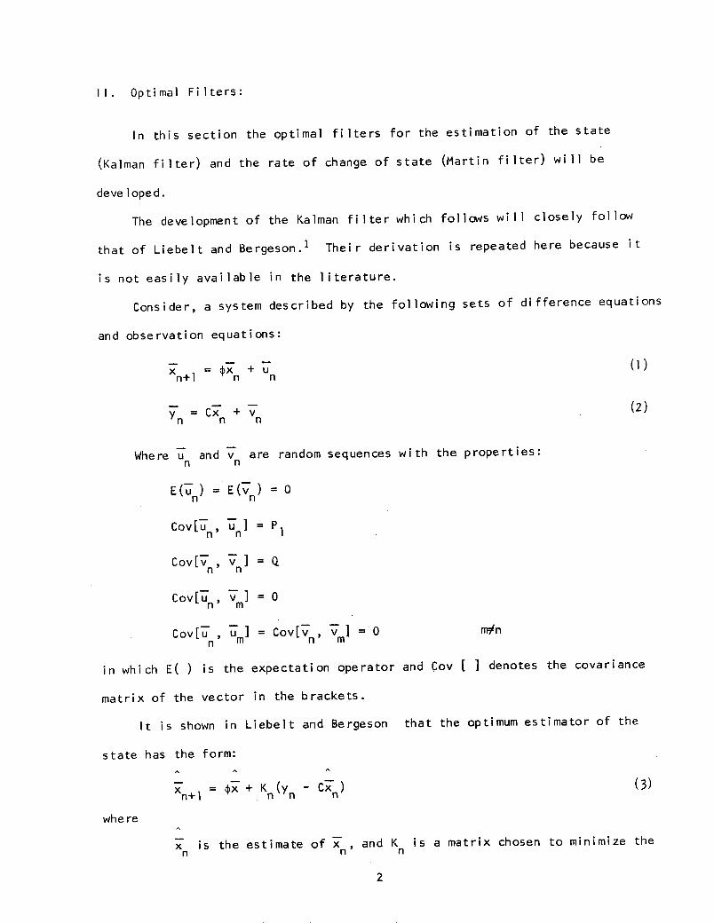
II. Optimal Filters:
In this section the optimal filters for the estimation of the state
(Kalman filter) and the rate of change of state (Martin filter) will be
developed.
The development of the Kalman filter which follows will closely follow
that of Liebelt and Bergeson.l Their derivation is repeated here because it
is not easily available in the literature.
Consider, a system described by the following sets of difference equations
and observation equations:
Xn+l --n x ny Cx + v
y =; Cxn + vn n n
Where un and vn are random sequences with the properties:
n nE(un)= E(Vn) =O
Cov[u, Un] = P
n n
Cov[u, nVm]
Cov[u , u ] = Cov[v vm] =0 mrnn m n' m
in which E( ) is the expectation operator and Cov [ ] denotes
matrix of the vector in the brackets.
It is shown in Liebelt and Bergeson that the optimum est
state has the form:
x-n+l X + Kn (Y - Cx)n~~l n n n
(1)
(2)
the covariance
imator of the
(3)
where
x is the estimate of x , and K is a matrix chosen to minimize then n n
2
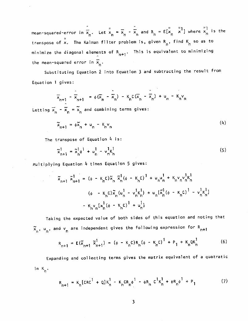
mean-squared-error in x Let x = x - x and R = E[x x ] where x is then n n n n
transpose of x. The Kalman filter problem is, given R , find K so as ton ~ n
minimize the diagonal elements of Rn+1 . This is equivalent to minimizing
the mean-squared error in xnn
Substituting Equation 2 into Equation 3 and subtracting the result from
Equation 1 gives:
x+ - x+1 =(Xn -x) -KC( -x) +u -Kyxn+l n+l n n n nn (n n n n n
Letting xn- x
nx and combining terms gives:
n n n(4)
Xn+l Xn + Un Knvn
The transpose of Equation 4 is:
n+l n n nn
Multiplying Equation 4 times Equation 5 gives:
xn+l xn+l = ( K - K n C) + K uv + Kn
1 (U' 1 1 -1 1 In n nn n n n n
Kn vnExn (4
- KnC)I + un]
Taking the expected value of both sides of this equation and noting that
x, un, and vn are independent gives the following expression for Rn+1
Rn+l = E(n+l Xn +l) = ( - KC)R n ( 1 + P + K K1 (6)
Expanding and collecting terms gives the matrix equivalent of a quatratic
in Kn
R1 + KCRn 1 + P1R Kn[CRC1 + Q]-K CR R C K +RR + P (7)n+l n n n n n n n 1
3
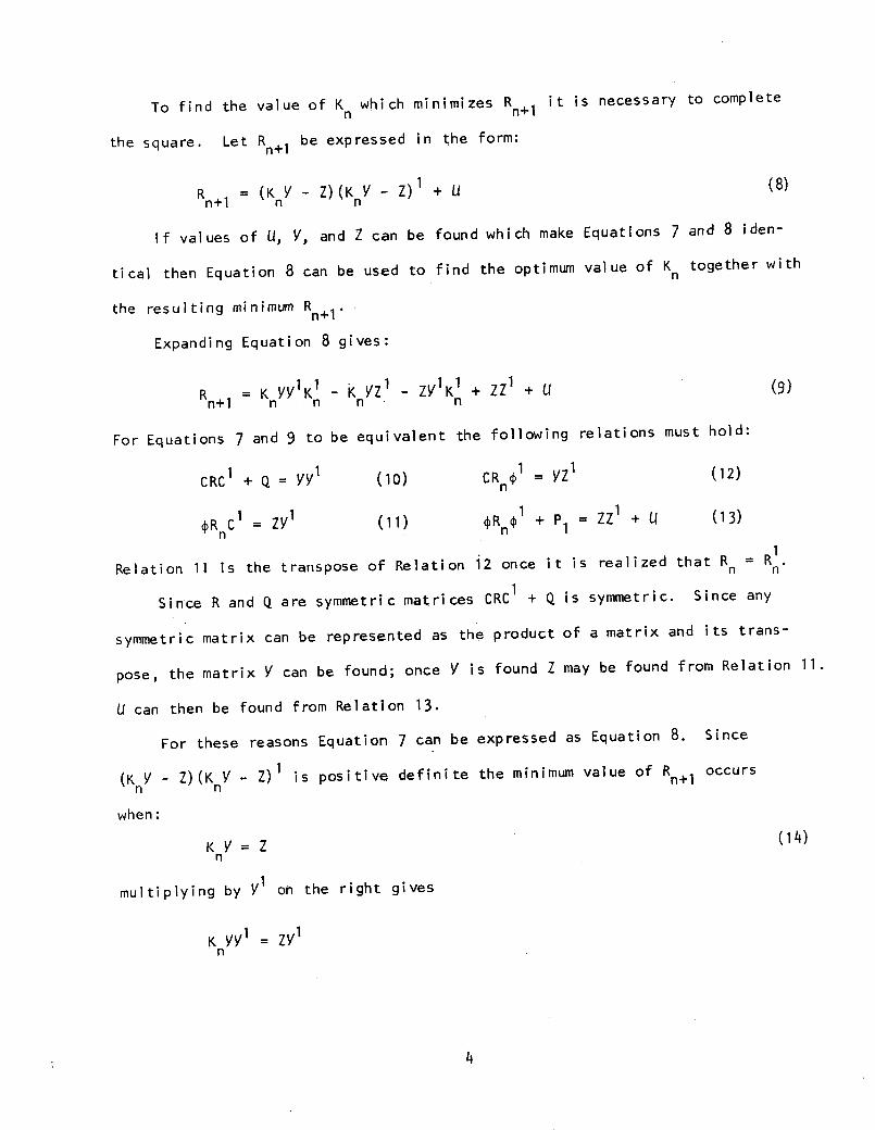
To find the value of K which minimizes Rn+l it is necessary to complete
the square. Let Rn+1 be expressed in the form:
Rn+1 = (KnY - Z)(KnY - Z)I + U
If values of U, YV, and Z can be found which make Equations 7
tical then Equation 8 can be used to find the optimum value of K
the resulting minimum Rn+1 .
Expanding Equation 8 gives:
(8)
and 8 iden-
together with
Rn+ = K -YY K1 ZYK + ZZ + Un+i n n n n
For Equations 7 and 9 to be equivalent the following relations must hold:
CRC1 + Q = YY1 (10) CR n1 = yZ1 (12)n
C1 = 1n
(11) pRn l + P1 = ZZ1 + Un I
1Relation 11 is the transpose of Relation i2 once it is realized that R = R
n n
Since R and Q are symmetric matrices CRC 1 + Q is symmetric. Since any
symmetric matrix can be represented as the product of a matrix and its trans-
pose, the matrix Y can be found; once Y is found Z may be found from Relation 11.
U can then be found from Relation 13.
For these reasons Equation 7 can be expressed as Equation 8. Since
(K Y - Z)(K Y - Z)1 is positive definite the minimum value of Rn+l occurs
when:
(14)KY= Zn
multiplying by Y1 on the right gives
K yyl = ZY1n
4
(9)
(13)
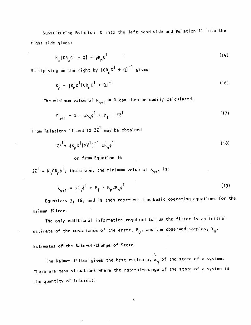
Substituting Relation 10 into the left hand side and Relation 11 into the
right side gives:
Kn[CR C + ] 1 = R C n n n
Multiplying on the right by [CR C1 + Q] gives
Kn = RnCI[CR C1 + Q] I
n n n
The minimum value of Rn+1 = U can then be easily calculated.
Rn+1
= U = Rnl + P1 - Z 1n+l nI
From Relations 11 and 12 ZZ1 may be obtained
ZZ = fRnC [yY ] CRnln n
(15)
(16)
(17)
(18)
or from Equation 16
ZZ = K CRnpl, therefore, the minimum value of Rn+1 is:n n n+1
R R =Rn + P K CR (19)
Equations 3, 16, and 19 then represent the basic operating equations for the
Kalman filter.
The only additional information required to run the filter is an initial
estimate of the covariance of the error, Ro, and the observed samples, Ynn
Estimates of the Rate-of-Change of State
The Kalman filter gives the best estimate, xn of the state of a system.
There are many situations where the rate-of-change of the state of a system is
the quantity of interest.
5
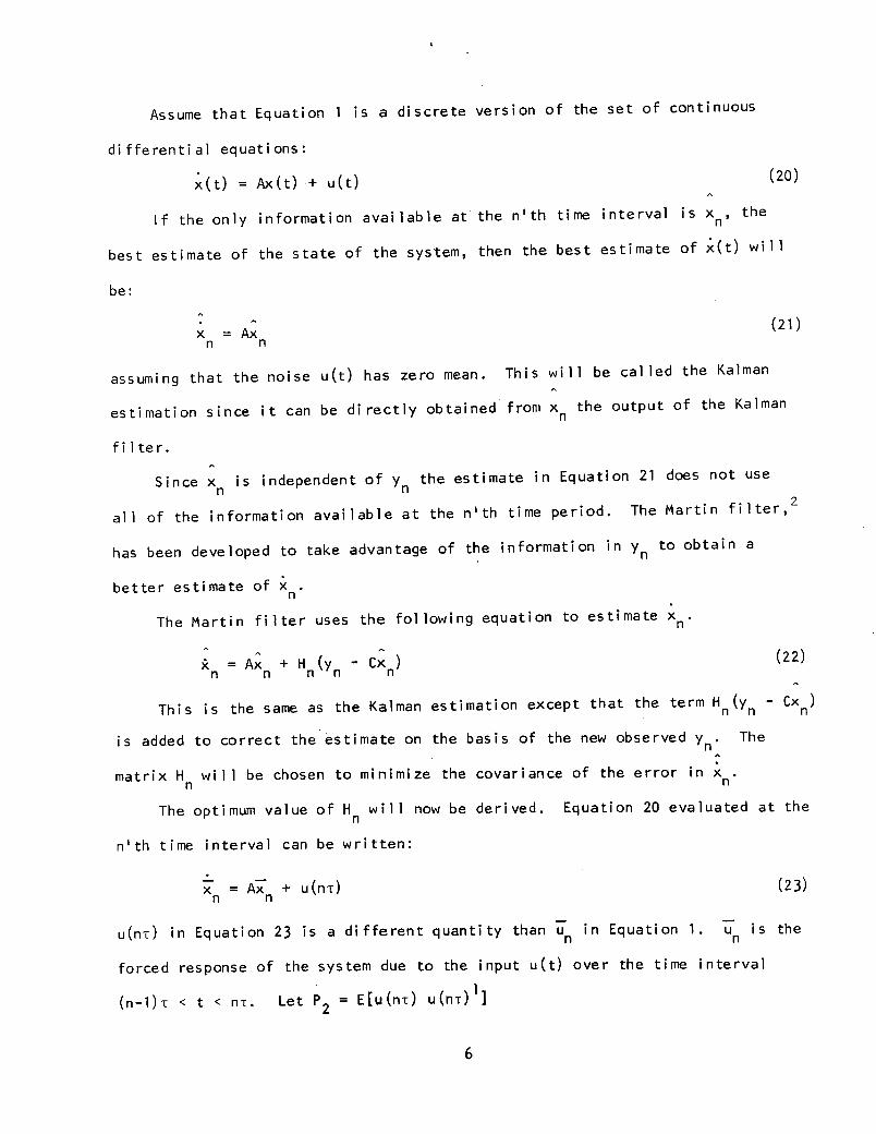
Assume that Equation 1 is a discrete version of the set of continuous
differential equations:
x(t) = Ax(t) + u(t) (20)
If the only information available at the n'th time interval is xn, the
best estimate of the state of the system, then the best estimate of x(t) will
be:
x = Ax (21)n n
assuming that the noise u(t) has zero mean. This will be called the Kalman
estimation since it can be directly obtained from xn the output of the Kalman
filter.
Since xn is independent of yn the estimate in Equation 21 does not use
all of the information available at the n'th time period. The Martin filter,2
has been developed to take advantage of the information in Yn to obtain a
better estimate of xn
The Martin filter uses the following equation to estimate xn
An = Axn + Hn(Yn CXn) (22)
This is the same as the Kalman estimation except that the term H (yn - Cx )
is added to correct the estimate on the basis of the new observed Yn. The
matrix H will be chosen to minimize the covariance of the error in x.n n
nThe optimum value of Hn will now be derived. Equation 20 evaluated at the
n'th time interval can be written:
Xn = Axn + u(nT) (23)
u(nr) in Equation 23 is a different quantity than un in Equation 1. u is then n
forced response of the system due to the input u(t) over the time interval
(n-l)T < t < nT. Let P2 = E[u(nT) u(nT)l]2
6
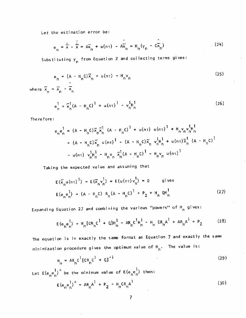
Let the estimation error be:
e x - x = Ax + u(nT) - A = H(yn n (24)n n n
Substituting yn from Equation 2 and collecting terms gives:
en = (A - H C) + u(n) - H v (25)
where x = x - xn n n
1 -1 1 1 1 1e = xn(A - H C) + u(nT) - v H (26)
nn n n
The re fore:
e e = (A - HC x xn (A -H C) 1 + u(nt) u(n-r) + Hvv H1nn n nn n n n nn
+ (A - H C) u(nT) - (A - H C)x v H1 + u(nT)3n (A - HC)n n n n nn n n
- u(nt) v1H 1 Hvn (A - H C) - H v u(nT)an n n n n
Taking the expected value and assuming that
1 1 1E(x u(nT) ) = E(xnv ) = E(u(nT)v ) = O gives
n nn n
E(ene) = (A - H C) R (A - HnC) + P + Hn QH (27)
Expanding Equation 27 and combining the various "powers" of Hngives:
E(enen) = H [CRC + Q]H - AR C H H CR A + AR A + P (28)nn n n n n n n n n 2
The equation is in exactly the same format as Equation 7 and exactly the same
minimization procedure gives the optimum value of Hn. The value is:
H = AR C [CR C + Q] (29)n n n
Let E(ene ) be the minimum value of E(ene ) then:
E(ene) = AR A + P - H CR A (30)En n n 2 n n
7
Comparison of Kalman and Martin Filters
Since the Martin filter can be reduced to the Kalman filter, Equation 21,
by letting Hn = O. The covariance of the error for the Kalman filter may be
obtained from Equation 30 by letting Hn O. Thus
(Kalan filter) Ee = A + P2 (31)(Kalman filter) E(ene AR A n
Letting A be the difference between Equations 31 and 30 gives:
A = H CR A1 (32)n n n
A is then the improvement in the covariance of the error caused by using
the Martin instead of the Kalman filter. In each application A will have to
be evaluated to see if the reduction in error is sufficient to justify the
additional complexity of the Martin filter.
The effectiveness of the Martin filter in estimating the rate of descent
of an aircraft is a function of the noise characteristics of the signals from
the pitch gyro and the radar altimeter. The next section of this report is
devoted to a study of these noises.
8
III. Noise Analysis:
In this section statistical characteristics of the measurement noise are
determined using real data determined during flight. The noise data was ob-
tained from NASA Guidance and Control Branch, Ames Research Center, Moffet
Field, California. A C8A, STOL aircraft was flown over level ground and
through several landings. The outputs of the pitch gyroscope and radar
altimeter were recorded on an Ampex FR-1300 seven channel FM tape recorder.
In the development of both the Kalman and Martin filters it was assumed
that the measurement noises were uncorrelated. That is E(vnvm) = 0 if nfm.
This is equivalent to saying that the autocorrelation function R(T) = 0 for
all T > T, where To is the time interval for the discrete Kalman filter.
Thus, it was necessary to obtain R(T) for both the altimeter and pitch gyroscope
noise. The power spectrum of the noise was obtained to determine if periodic
signals such as power supply hum were present in the noise. Any such periodic
noise must be filtered out if R(T) is to approach zero as T tends to infinity.
In both the Kalman and Martin filters quadratic loss functions of the form
E(x x ) are minimized. It is well known that the optimum filter is not depen-
dent on the shape of the loss function if the noise is Gaussian. For this
reason the first order density function was obtained to determine if the noise
was Gaussian.
The only measurement noise parameters actually used in either filter are
the diagonal elements of the Q matrix. These are the variances of the altimeter
noise and the pitch gyroscope noise. These were obtained by evaluating R(-) at
T = 0 and as a check were obtained from the density functions.
The signals of the altimeter and pitch gyroscope were recorded by an on-
board, FM tape recorder. They contain the real values of the altitude and pitch
9
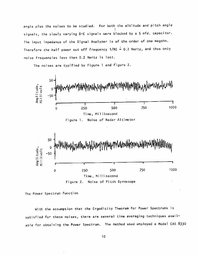
angle plus the noises to be studied. For both the altitude and pitch angle
signals, the slowly varying D-C signals were blocked by a 5 mfd. capacitor.
The imput impedance of the Signal Analyzer is of the order of one megohm.
Therefore the half power cut off frequency 1/RC = 0.2 Hertz, and thus only
noise frequencies less than 0.2 Hertz is lost.
The noises are typified by Figure 1 and Figure 2.
50-
ac0 01
-- = -50
I I I I I0 250 500 750 1000
Time, Millisecond
Figure 1. Noise of Radar Altimeter
50
4-J 0
., -50
Q.-
0 250 500 750 1000
Time, Millisecond
Figure 2. Noise of Pitch Gyroscope
The Power Spectrum Function
With the assumption that the Ergodicity Theorem for Power Spectrums is
satisfied for these noises, there are several time averaging techniques avail-
able for obtaining the Power Spectrum. The method used employed a Model CAS 8330
10
Signal Analyzer and a specialized hybrid computing system. The Algorithm and
the curves are presented in Figures 3, 4, and 5. In the curves only relative
amplitudes are given.
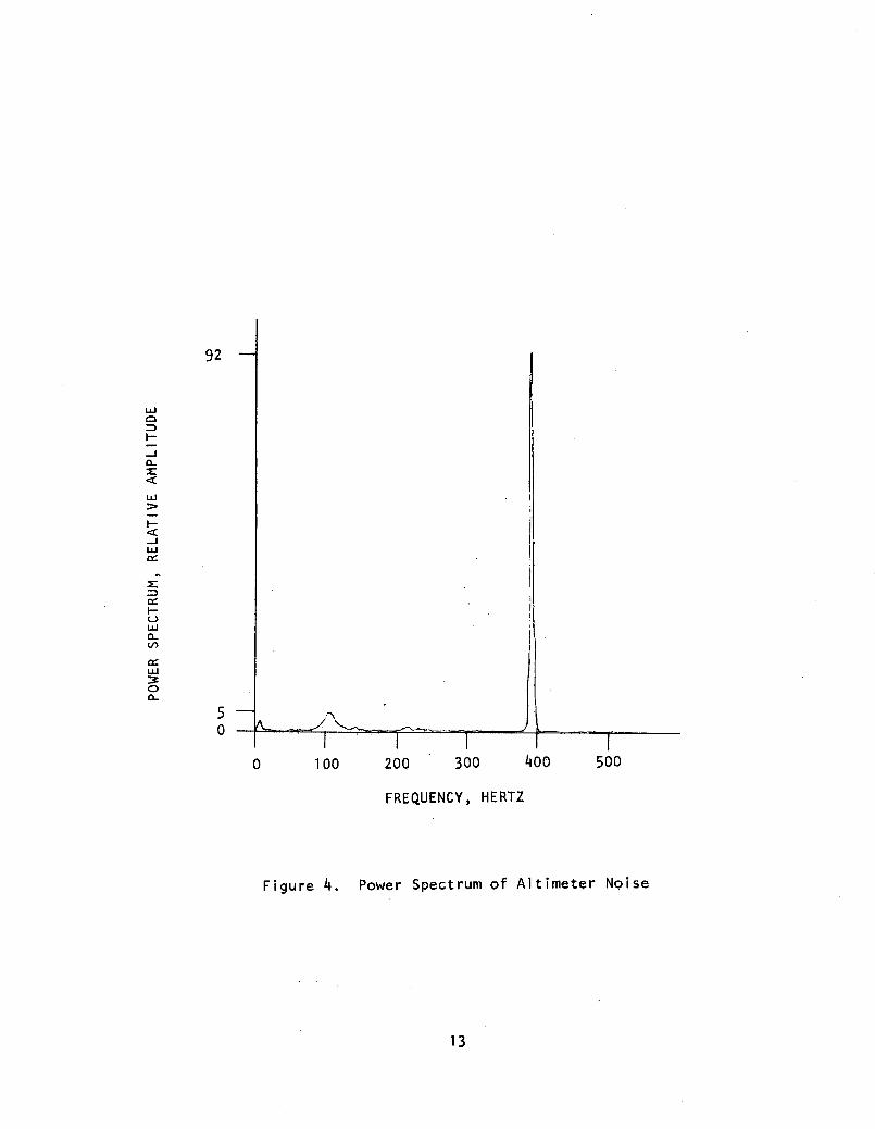
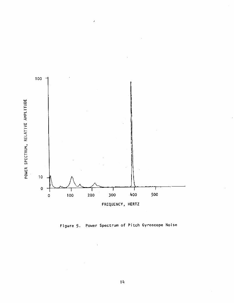
From Figure 4 and Figure 5 it is clear that the power spectra of both
noises have significant components at 400 Hz and negligible components at
frequencies larger than 400 Hz. Since the FM tape recorder and the aircraft
instruments were all driven from the 400 Hz power available in the aircraft
it is not possible to determine if this large 400 Hz component was present
in the altimeter and pitch gyro outputs, or was introduced by the FM tape
recorder. In any case it can easily be removed. Before the autocorrelation
function, R(rT), was calculated the 400 Hz component was removed with an electron-
ic low-pass filter which suppressed it 40 d.b.
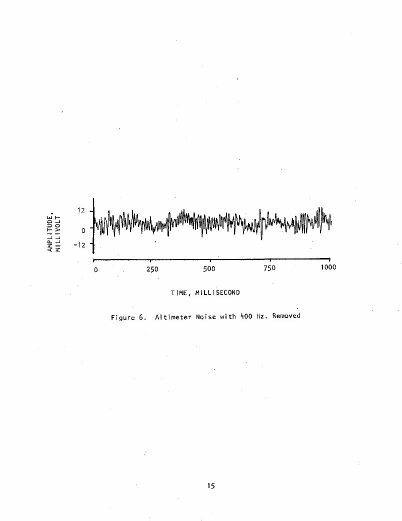
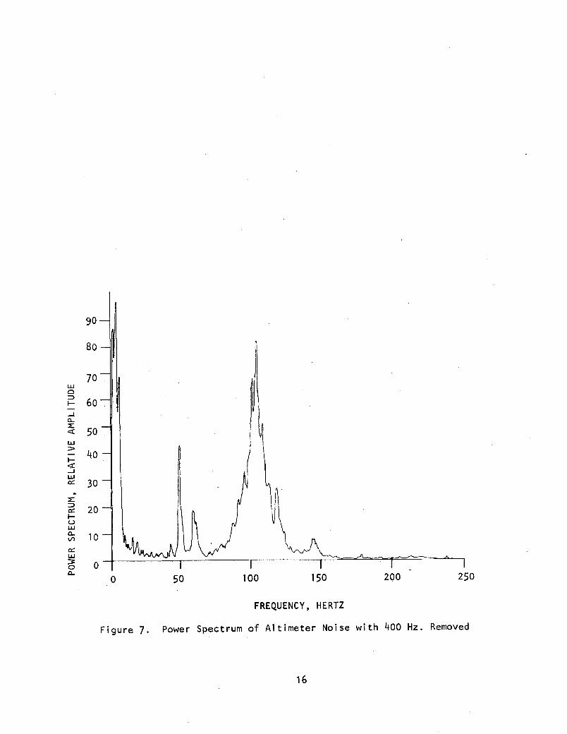
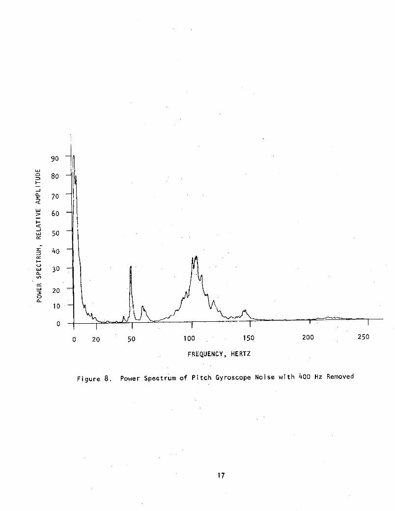
These filtered noises, are typified in Figure 6 and Figure 9. Their power
spectrums are shown in Figure 7 and Figure 8.
11
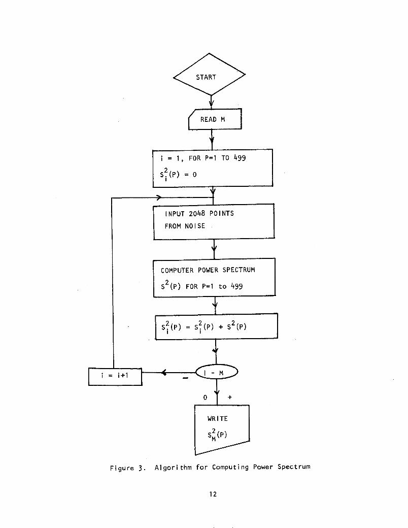
Figure 3. Algorithm for Computing Power Spectrum
12
INPUT 2048 POINTS
FROM NOISE
COMPUTER POWER SPECTRUM
S (P) FOR P=1 to 499
92
LU
-
ii
-
V3
i:i
LUw0
a-
50
0 100 200 300 400 500
FREQUENCY, HERTZ
Figure 4. Power Spectrum of Altimeter Noise
13
100
10
0
0 100 200 300 400 500
FREQUENCY, HERTZ
Figure 5. Power Spectrum of Pitch Gyroscope Noise
14
I-
-JCLi
I--LJ
_I
L)
a-w
W
0
a-
:wC)
CL
12Lul--
I-r
'-> o
-M -12<~-
. , I .. · 1
0 250 500 750 1000
TIME, MILLISECOND
Figure 6. Altimeter Noise with 400 Hz. Removed
15
90
80
70
6o- 60
50w
30-
20 -
Q-
w
1 30
n-
Q~~K_0 50 100 150 200 250
FREQUENCY, HERTZ
Figure 7. Power Spectrum of Altimeter Noise with 400 Hz. Removed
16
90
o 80 -
X 70
w60
50
40 -
L 30a-
20
0 10
0 20 50 100 150 200 250
FREQUENCY, HERTZ
Figure 8. Power Spectrum of Pitch Gyroscope Noise with 400 Hz Removed
17
12
30-
E d ~E -12
JI ... I 'I I ,
0 250 500 750 1000
Time, Millisecond
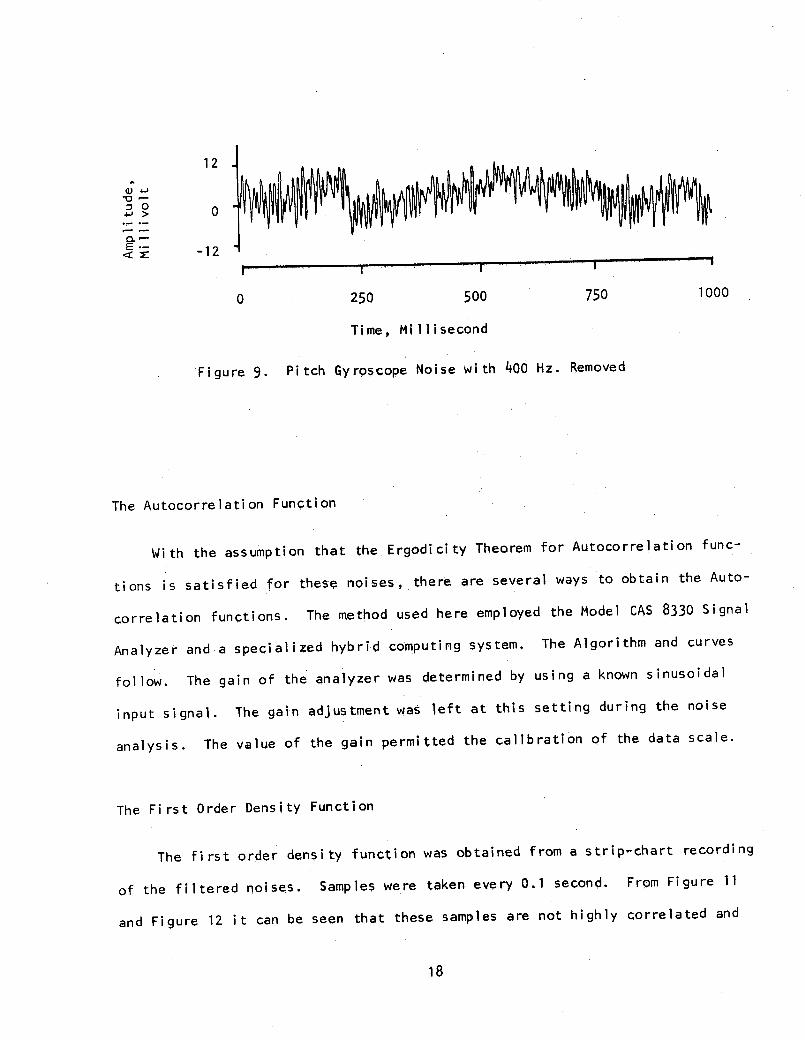
Figure 9. Pitch Gyroscope Noise with 400 Hz. Removed
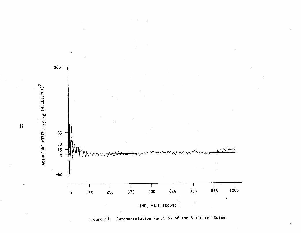
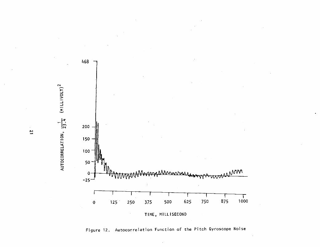
The Autocorrelation Function
With the assumption that the Ergodicity Theorem for Autocorrelation func-
tions is satisfied for these noises, there are several ways to obtain the Auto-
correlation functions. The method used here employed the Model CAS 8330 Signal
Analyzer and a specialized hybrid computing system. The Algorithm and curves
follow. The gain of the analyzer was determined by using a known sinusoidal
input signal. The gain adjustment was left at this setting during the noise
analysis. The value of the gain permitted the calibration of the data scale.
The First Order Density Function
The first order density function was obtained from a strip-chart recording
of the filtered noises. Samples were taken every 0.1 second. From Figure 11
and Figure 12 it can be seen that these samples are not highly correlated and
18
START
READ T, ,. N
Ii = i+l
"F
+I C(P) = C(P) + Ci(P)
D . i-N
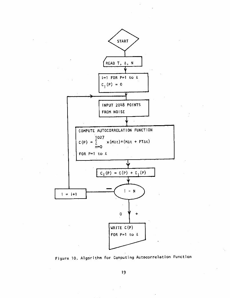
Figure 10. Algorithm for Computing Autocorrelation Function
19
i=l FOR P=1 to 2
C i(P) = 0
1INPUT 2048 POINTS
FROM NOISE
COMPUTE AUTOCORRELATION FUNCTION
'1027C(P) = I x(MAt)*(MAt + PTAt)
m=O
FOR P=1 to 9
I
I
0
cA
~~
~~
~~
~~
~~
-~~
~4
EL
, OL
0 0
-Z
C(
LI
CC
o cZ
?, -
~~
~0
Li
U)
0
0 LA
O
~~
~~
nO
0%
D~
~u
c~
~~
~~
J I~
~~
~
I~
~ ~
~ ~
~~
, c
20
o 0
0 0
o uL
0 U
.
000U-0C)
r-U-N
0w()C
O-0
-
IE.
wl
I-oL
Lu?
O
-c)
-L
n
(-4
Lfl
N
-014
's
onI
z(llOA
I111W)
£'Z 'N
O)I£V
13d30 fLnv
z Iniiw
21
£)00Utn-C ac4
CL4J c.a-4.,.c 0L
0)
LL
co%D
-:r
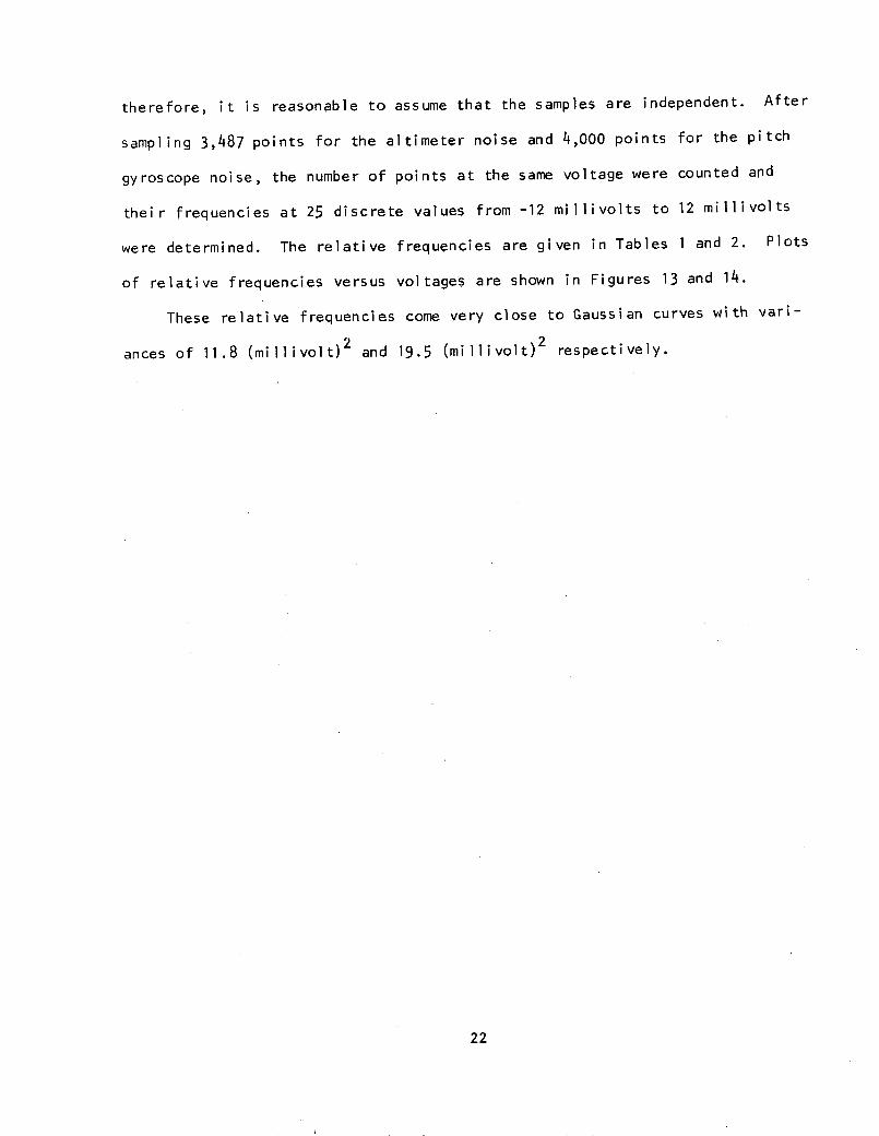
therefore, it is reasonable to assume that the samples are independent. After
sampling 3,487 points for the altimeter noise and 4,000 points for the pitch
gyroscope noise, the number of points at the same voltage were counted and
their frequencies at 25 discrete values from -12 millivolts to 12 millivolts
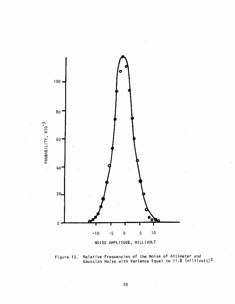
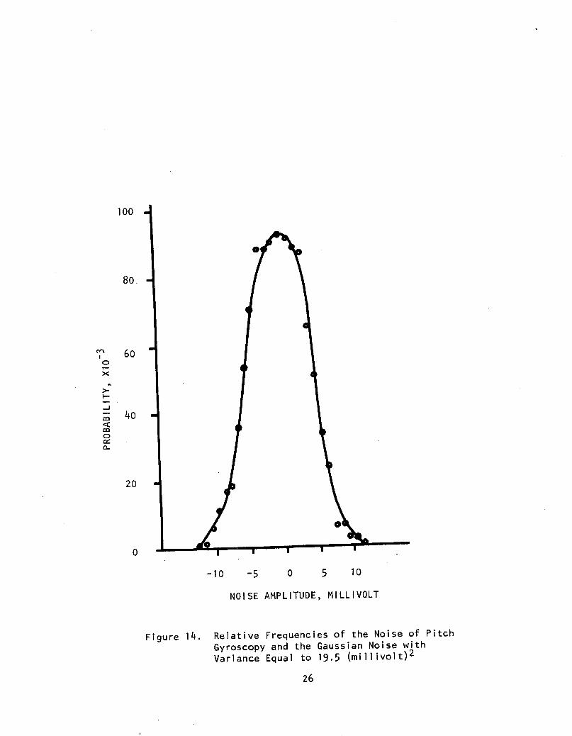
were determined. The relative frequencies are given in Tables 1 and 2. Plots
of relative frequencies versus voltages are shown in Figures 13 and 14.
These relative frequencies come very close to Gaussian curves with vari-
ances of 11.8 (millivolt)2 and 19.5 (millivolt)2 respectively.
22
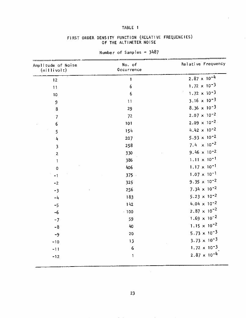
TABLE 1
FIRST ORDER DENSITY FUNCTION (RELATIVE FREQUENCIES)OF THE ALTIMETER NOISE
Number of Samples = 3487
Amplitude of Noise No. of Relative Frequency(millivolt) Occurrence
2.87 x 10- 4
1.72 x 10⁻³
1.72 x 10⁻³
3.16 x 10⁻³
8.36 x 10⁻³
2.07 x 10⁻²
2.09 x 10⁻²
4.42 x 10- 2
5.93 x 10⁻²
7.4 x 10⁻²
9.46 x 10⁻²
1.11 x 10⁻¹
1.17 x 10-'1
1.07 x 10'1
9.35 x 10⁻²
7.34 x 10⁻²
5.23 x 10- 2
4.04 x 10'2
2.87 x 10⁻²
1.69 x 10⁻²
1.15 x 10'2
5.73 x 10⁻³
3.73 x 10⁻³
1.72 x 10⁻³
2.87 x 10- 4
12
11
10
9
8
7
6
5
4
3
2
1
0
-1
-2
-3
-4
-5
-6
-7
-8
-9
-10
-11
-12
1
6
6
11
29
72
101
154
207
258
330
386
406
375
325
256
183
1 42
100
59
40
20
13
6
1
23
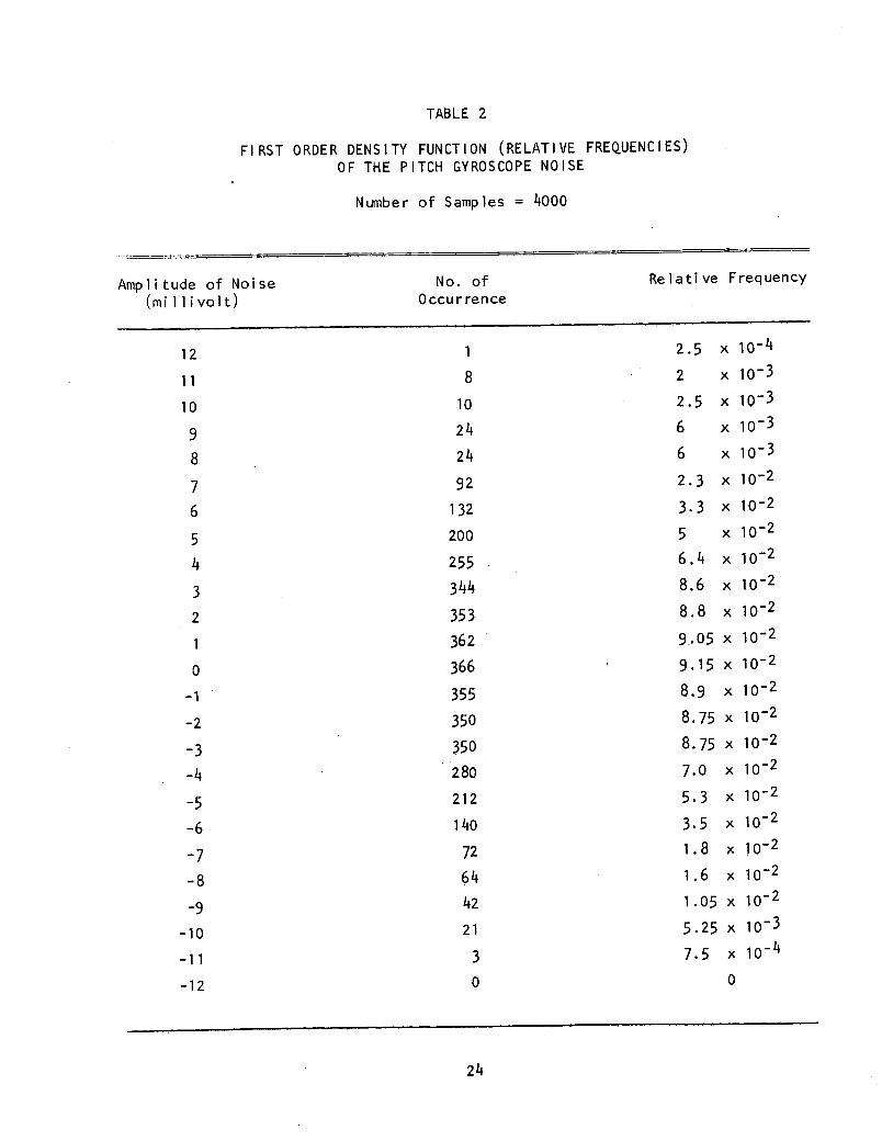
TABLE 2
FIRST ORDER DENSITY FUNCTION (RELATIVE FREQUENCIES)OF THE PITCH GYROSCOPE NOISE
Number of Samples = 4000
Amplitude of Noise No. of Relative Frequency(millivolt) Occurrence
12
11
10
98
76
5
4
32
1
0
-1
-2
-3
-4
-5
-6
-7
-8
-9
-10
-11
-12
1
8
10
24
24
92
132
200
255
344
353
362
366
355
350
350
280
212
140
72
64
42
21
3
0
2.5
2
2.5
6
6
2.3
3.3
5
6.4
8.6
8.8
9.05
9.15
8.9
8.75
8.75
7.0
5.3
3.51.8
1.6
1.05
5.25
7.5
x 10-4
x 10-3
x 10-3
x 10-3
x 10-3
x 10-2
x 10-2
x 10-2
x 10-2
x 10-2
x 10-2
x 10-2
x 10-2
x 10-2
x 10-2
x 10-2
x 10-2
x 10-2
x 10- 2
x 10-2
x 10 - 2
x 10-3
x 10- 4
0
100
80
0
> '60"
4o
2O.
0
-10 -5 0 5 10
NOISE AMPLITUDE, MILLIVOLT
Figure 13. Relative Frequencies of the Noise of Altimeter andGaussian Noise with Variance Equal to 11.8 (millivolt)2
25
100
80.
2 60060
4o
2020
-10 -5 0 5 10
NOISE AMPLITUDE, MILLIVOLT
Figure 14. Relative Frequencies of the Noise of PitchGyroscopy and the Gaussian Noise withVariance Equal to 19.5 (millivolt)2
26
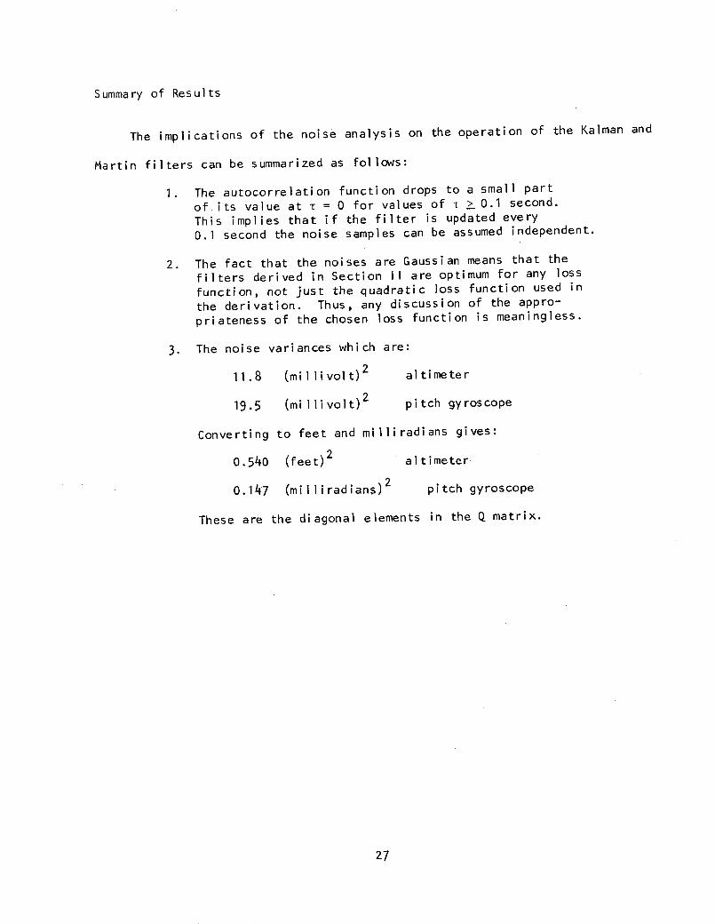
Summary of Results
The implications of the noise analysis on the operation of the Kalman and
Martin filters can be summarized as follows:
1. The autocorrelation function drops to a small partof.its value at T = 0 for values of T > 0.1 second.This implies that if the filter is updated every0.1 second the noise samples can be assumed independent.
2. The fact that the noises are Gaussian means that thefilters derived in Section II are optimum for any lossfunction, not just the quadratic loss function used inthe derivation. Thus, any discussion of the appro-priateness of the chosen loss function is meaningless.
3. The noise variances which are:
11.8 (millivolt)2 altimeter
19.5 (millivolt)2 pitch gyroscope
Converting to feet and milliradians gives:
0.540 (feet)2 altimeter
0.147 (milliradians)2 pitch gyroscope
These are the diagonal elements in the Q matrix.
27
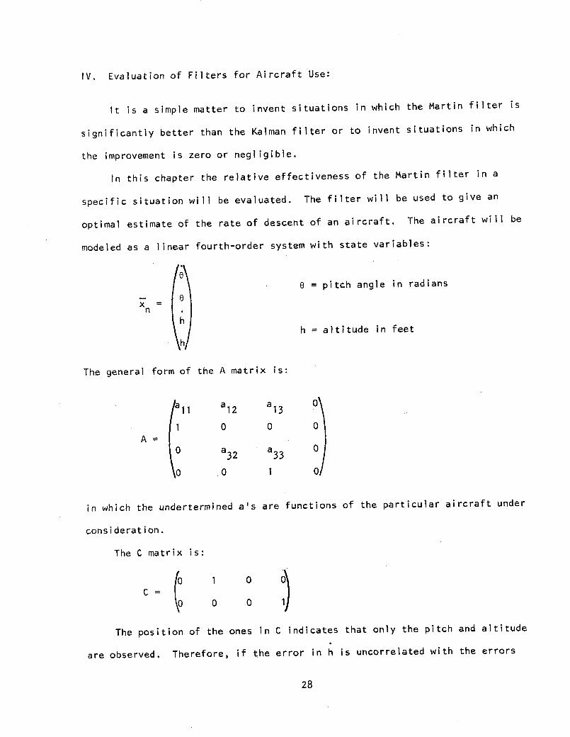
IV. Evaluation of Filters for Aircraft Use:
It is a simple matter to invent situations in which the Martin filter is
significantly better than the Kalman filter or to invent situations in which
the improvement is zero or negligible.
In this chapter the relative effectiveness of the Martin filter in a
specific situation will be evaluated. The filter will be used to give an
optimal estimate of the rate of descent of an aircraft. The aircraft will be
modeled as a linear fourth-order system with state variables:
e = pitch angle in radians
x =n
h = altitude in feet
The general form of the A matrix is:
all a12 aO3
0 0 0A=
o a3 2
a 0O a32 a33
o0 1 0
in which the undertermined a's are functions of the particular aircraft under
consideration.
The C matrix is:
1 0
0 0 1
The position of the ones in C indicates that only the pitch and altitude
are observed. Therefore, if the error in h is uncorrelated with the errors
28
in both e and h, 7 n will give no information about h, and the Martin filter
will give the same estimate of h as the Kalman filter.
In terms of matrices this implies that if R is diagonal then the fourth
row in H will have all zero terms and no correction in the Kalman estimaten
of h will occur. Multiplying the matrices in H and keeping track of the
zeros in C and Rn
shows that this is true if R is diagonal. Ro0 the initial
Rn, can reasonably be assumed diagonal since there is no reason that errors
in 3, 0, h, and h should be correlated. R will not be diagonal in generaln
since errors in one state variable will propagate into the other state vari-
ables through the action of the 9 matrix.
Thus it is to be expected that the Martin filter will not be a significant
improvement until sufficient time has passed for Rn to develop significant
terms.
If P = 0 then R will tend to zero as time increases and it is possiblen
that no time interval will exist in which the Martin filter is a significant
improvement over the Kalman filter.
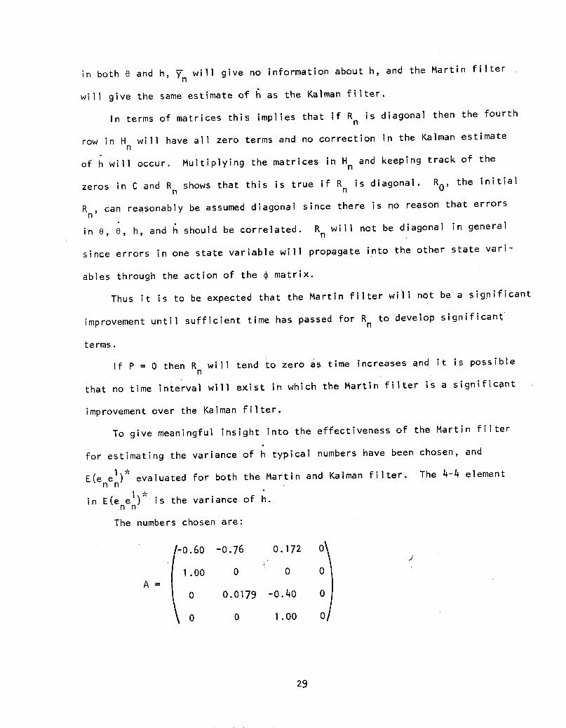
To give meaningful insight into the effectiveness of the Martin filter
for estimating the variance of h typical numbers have been chosen, and
E(ene ) evaluated for both the Martin and Kalman filter. The 4-4 element
in E(ene ) is the variance of h.
The numbers chosen are:
-0.60 -0.76 0.172 0
1.00 0 0 0A=
0 0.0179 -0.40 0
0 0 1.00 0
29
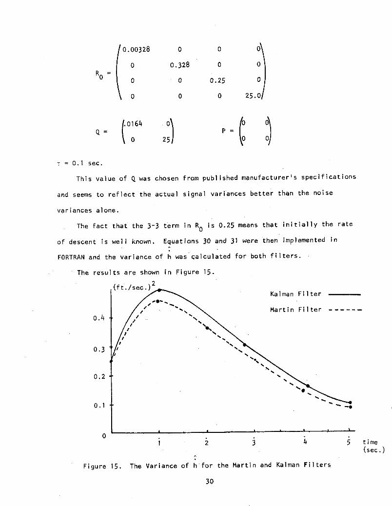
0.00328
0RO =
0
0
0
0.328
0
0
0
0
0.25
0
O
25.0
Q (°0164
0 25
T = 0.1 sec.
This value of Q was chosen from published manufacturer's specification!
and seems to reflect the actual signal variances better than the noise
variances alone.
The fact that the 3-3 term in RO is 0.25 means that initially the rate
of descent is well known. Equations 30 and 31 were then implemented in
FORTRAN and the variance of h was calculated for both filters.
The results are shown in Figure 15.
,(ft./sec.)2.
0.4
0.3
0.2
0.1
01 2
S5
Kalman Filter
Martin Filter
i4
Figure 15. The Variance of h for the Martin and Kalman Filters
30
time(sec.)
P =
From Figure 15 it can be seen that for t > 2 seconds the Martin filter
is approximately 12 percent better than the Kalman filter. For t > 5 both
filters are so accurate that there is no reason to implement the more com-
plex Martin filter. If P1 $ 0 then R would not approach 0 and the 12
percent improvement of the Martin filter would continue to be important
for all times.
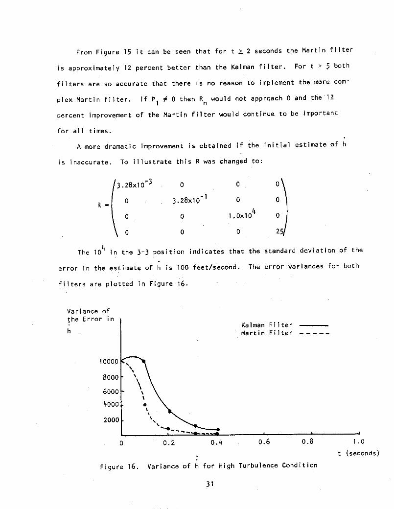
A more dramatic improvement is obtained if the initial estimate of h
is inaccurate. To illustrate this R was changed to:
3.28xlO03
R= 0
0
0
0
3.28xl QO 1
0
0
0
0
1 0x104
0
0
0
0
25
The 104 in the 3-3 position indicates that the standard deviation of the
error in the estimate of h is 100 feet/second. The error variances for both
filters are plotted in Figure 16.
Variance ofthe Error in
h
10000
8000
6000
4000
Kalman FilterMartin Filter
0 0.2 0.4 0.6 0.8
Figure 16. Variance of h for High Turbulence Condition
31
1.0
t (seconds)
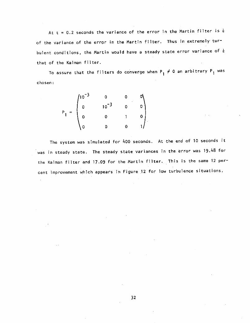
At t = 0.2 seconds the variance of the error in the Martin filter is ¼
of the variance of the error in the Martin filter. Thus in extremely tur-
bulent conditions, the Martin would have a steady state error variance of ¼
that of the Kalman filter.
To assure that the filters do converge when P1 # 0 an arbitrary P1 was
chosen:
-3
0 10- 3 0 0P
=
0 1 01 0 0 1
0 0 0 1
The system was simulated for 400 seconds. At the end of 10 seconds it
was in steady state. The steady state variances in the error was 19.48 for
the Kalman filter and 17.09 for the Martin filter. This is the same 12 per-
cent improvement which appears in Figure 12 for low turbulence situations,
32
V. Summary:
The purpose of this grant was the development of a digital filter for the
optimal estimation of the rate of descent of aircraft. A filter, called the
Martin filter, was developed which gives the optimum estimate of the rate of
change of the state of the system. In situations where the error variances
are small the Martin filter will have an error variance of 88 percent of the
Kalman filter. If the error variances are large, such as in very turbulent
air, it will produce error variance of 25 percent of those produced by the
Kalman filter. These error variances are approximate. More accurate results
will not be possible until more data on the P matrix caused by various tur-
bulence conditions is known.
33
VI. References:
1. Liebelt, P. B. and J. E. Bergeson, "The Generalized Least Square andWiener Theories with Applications to Trajectory Prediction," BoeingDocument No. DZ-90167, May 1962.
2. Martin, J. C., "Minimum Variance Estimates of Signal Derivatives,"NASA Research Grant NGR-41-001-24, December 1970.
34