COLGATE UNIVERSITY

The Impact of Age on Baseball Players’

Performance How Was this Altered During the Steroid Era

Nikolas Ahrendt Furnald

Advised by Professor Michael E. O’Hara

4/16/2012

Keywords: Baseball, (Price) Elasticity of Demand, First differences, Sports Economics

JEL codes: L83

This project addresses the impact of age on player performance in baseball. Building on

prior literature, this paper is the first on the impact of aging in baseball to use Wins Above

Replacement. On top of this, this study examines the impact of the steroid era on aging. This

paper finds that steroid era allowed players to peak at a higher level as well as an older age

(29.057 versus 27.655).

1

1 Introduction

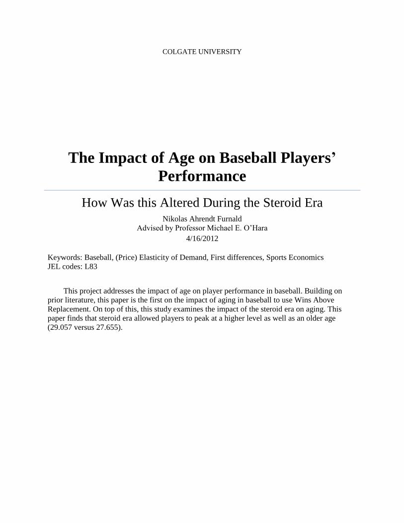
In 2010, Major League Baseball had revenues of $7 billion in one season and this month

the Los Angeles Dodgers were purchased for $2.15 billion. These two figures are just examples

of the various statistics that one can draw on to demonstrate the massive amount of money that is

involved in Major League baseball, especially today. Building on this idea, as one can see from

Table 1, three of the five largest contracts ever were signed this offseason. When looking at these

massive deals, an important aspect to consider is the age of the players involved in the deal and

the length of the contract. While all of these players are at the peak of careers when these

contracts are signed, it is very important for a Major League general manager to additionally

consider the value that they will be able to get out of their players during the final years of these

contracts.

The objective of this project is to further the understanding of how age impacts a baseball

player’s performance. More specifically, the goal of this paper is to look at a new variable, Wins

Above Replacement1 (WAR) as a measure of performance whereas older studies uses statistics

that only look at one portion of a player’s contribution to his team, since most studies in this field

only focus on offensive statistics.

This paper specifically investigates whether the steroid era changed this aging curve. The

steroid era is defined as the period from 1994-2004, where there is a great deal of evidence that a

1 Win Above Replace is an all-encompassing statistic which incorporates all aspect of a player’s value to his team. A

more detailed explanation of this statistic is on page six.

Name Length Value Date Age

Alex Rodriguez 10 $275 million 12/13/2007 31

Alex Rodriguez 10 $252 million 2001 25

Albert Pujols 10 $240 million 1/5/2012 32

Prince Fielder 9 $213 million 1/25/2012 27

Joey Votto 10 $225 million 4/2/2012 28

Table 1: Largest Contracts in MLB History

2

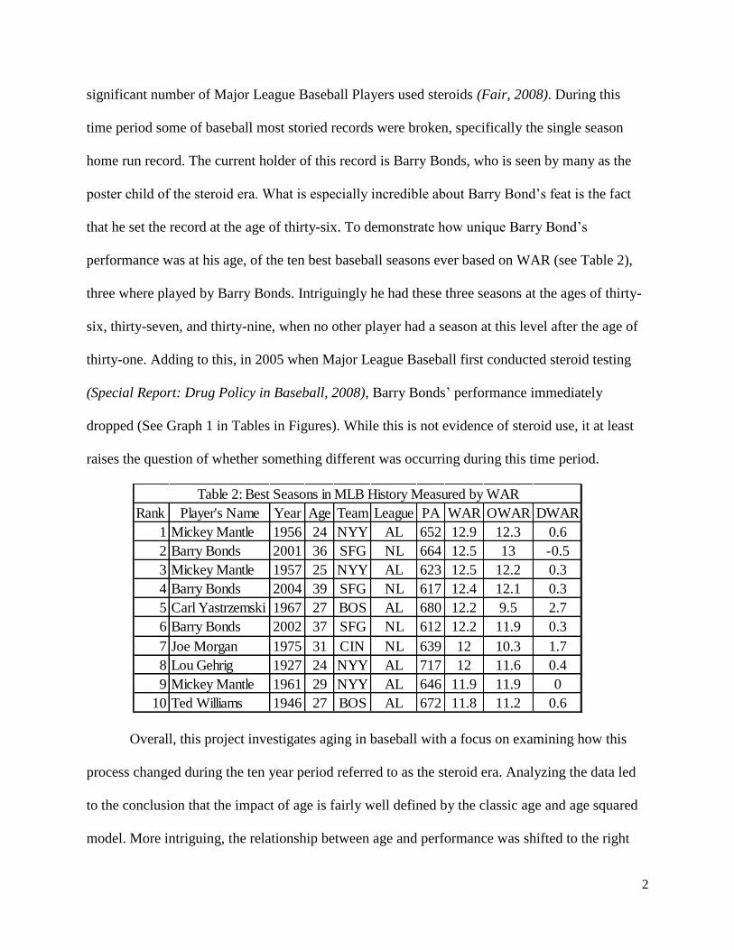
significant number of Major League Baseball Players used steroids (Fair, 2008). During this

time period some of baseball most storied records were broken, specifically the single season

home run record. The current holder of this record is Barry Bonds, who is seen by many as the

poster child of the steroid era. What is especially incredible about Barry Bond’s feat is the fact

that he set the record at the age of thirty-six. To demonstrate how unique Barry Bond’s

performance was at his age, of the ten best baseball seasons ever based on WAR (see Table 2),

three where played by Barry Bonds. Intriguingly he had these three seasons at the ages of thirty-

six, thirty-seven, and thirty-nine, when no other player had a season at this level after the age of

thirty-one. Adding to this, in 2005 when Major League Baseball first conducted steroid testing

(Special Report: Drug Policy in Baseball, 2008), Barry Bonds’ performance immediately

dropped (See Graph 1 in Tables in Figures). While this is not evidence of steroid use, it at least

raises the question of whether something different was occurring during this time period.

Overall, this project investigates aging in baseball with a focus on examining how this

process changed during the ten year period referred to as the steroid era. Analyzing the data led

to the conclusion that the impact of age is fairly well defined by the classic age and age squared

model. More intriguing, the relationship between age and performance was shifted to the right

Rank Player's Name Year Age Team League PA WAR OWAR DWAR

1 Mickey Mantle 1956 24 NYY AL 652 12.9 12.3 0.6

2 Barry Bonds 2001 36 SFG NL 664 12.5 13 -0.5

3 Mickey Mantle 1957 25 NYY AL 623 12.5 12.2 0.3

4 Barry Bonds 2004 39 SFG NL 617 12.4 12.1 0.3

5 Carl Yastrzemski 1967 27 BOS AL 680 12.2 9.5 2.7

6 Barry Bonds 2002 37 SFG NL 612 12.2 11.9 0.3

7 Joe Morgan 1975 31 CIN NL 639 12 10.3 1.7

8 Lou Gehrig 1927 24 NYY AL 717 12 11.6 0.4

9 Mickey Mantle 1961 29 NYY AL 646 11.9 11.9 0

10 Ted Williams 1946 27 BOS AL 672 11.8 11.2 0.6

Table 2: Best Seasons in MLB History Measured by WAR

3

and upward, as player’s bodies began to deteriorate at a faster rate because the aging process

became more drastic during the steroid era.

2 Literature Review: Background in Baseball Economics

The majority of economic research done on baseball has focused on labor markets,

because there is a large amount of data availability on performance (Scully, 1974). Often

economists use baseball as a place to test their labor markets theories. When discussing these

theories, baseball economic studies need to use a statistic which represents a player’s

performance for his team.

Batting average, denoted AVG, is used in most studies on position players, yet it is not a

good proxy for player performance. Economists see this statistic as volatile (Bradbury, 2007)

because it is dependent on aspects of the game that are out of a player’s control including the

opponent’s defensive ability (Bradbury, 2011). As a result, AVG does a poor job predicting

future performance and even shows a weak correlation with runs scored by a team (Bradbury,

2011). Due to these findings, baseball economists have shifted their focus to other statistics such

as on-base percentage plus slugging percentage (OPS) for hitter, a statistic has been shown to be

strongly correlated with actual runs and is a better predictor of future performance (Sommers,

1992).

Another area which has been discussed is the impact of fielding abilities on a player’s

value to his team. Unfortunately, most studies do not consider fielding since most defensive

statistics are not considered a good proxy for a player’s performance (Bradbury, 2011). A good

example of a defensive statistic with this issue is errors2. Since errors are subjective and are

2 An Error is a mistake by a fielder that allows a batter to reach base, a runner to advance an extra base, or allows an

at bat to continue after the batter should have been put out. This statistic is based on the judgment of the official

scorer (Baseball Reference).

4

based solely on a player’s ability to field balls hit directly to him, this statistic does not fully

represent a player’s defensive ability (Bradbury, 2011). Even though these older statistics have

issues, prior research has discussed the importance of fielding to understanding the value of a

player, and in particular on comparing the performance of players at different positions

(Bradbury, 2011).

Moving onward, another area of baseball economics literature is on understanding the

aging process. The majority of work on this area has used a fairly simple age and aged squared

model (Scully G. , 1974): a player will develop skills and increase performance at a diminishing

rate until a certain age, when the effect of growing older will begin to take a toll on the player’s

body, after which a player’s performance will begin decline (Bradbury, 2011).

The most debated topic in baseball aging papers is that players that go below the

replacement level of performance end their careers. Since studies try to track the performance of

players over an extended career, they usually remove any player who does not meet the set level

of career at-bats. This creates a sampling bias as the players who have extended careers are of a

higher level of talent. As a result, a big factor in determining the impact of age on a player’s

performance is which players to include the study (Berna Demiralp, 2010). One way is to find

every player’s individual peak year and then average this number. Unfortunately, this method

would lead to earlier peaks, because players suffer from non-age related injuries. Another

method is to look just at players who have long careers and assume that the effect of aging is the

same for both high-level and marginal players (Berna Demiralp, 2010). As a result, this debate is

an important aspect of creating this project’s dataset.

A major development in sports economics over the last two decades is the use of

performance enhancing drugs. A variety of economic papers has been written on the subject (for

5

example Evans-Brown & McVeigh March 2009, Fisher 2008, and Thurston 1990). The most

important to this paper is an article headlined “Builds Muscles, Shrinks Careers”. This article

quotes Dr. James Andrews, the most renowned orthopedist in baseball, to establish the concept

that steroids increase an athlete’s muscle mass, but cause longer-term issues that could lead

athlete’s career to be shortened (Manning, 2002).

Moving from general sports to the specific focus of baseball, there is a vast amount that

has been written on the steroid era3. To begin digging into this literature, the issue of why a

player would use steroids has been looked at by a variety of papers. For example, Evan

Osborne’s (2005) Performance-Enhancing Drugs: An Economic Analysis looked at the financial

advantage of a baseball player to use steroids and Grossman et al. (2007) Steroids and Major

League Baseball used game theory to approach this same dilemma. On top of this, the impact of

the steroid era on home runs has also been extensively covered by (Tobin, 2007), (Petersen,

Jung, & Eugene, 2008), (Winfree, 2007), and (Vany, 2010). Finally, Schmotzer et al. (2008)

looked at whether players implicated in the Mitchell Report performed above other players

during the steroid era, finding that known steroid users did have an advantage over other players

all else equal.

Intriguingly, there is less literature on how the aging of players was affected by the

steroid era. The most helpful paper on this topic is Ray Fair’s (2005) Estimated Age Effects in

Baseball which adds to the literature by creating a model that looked at peak age and how

performance deviates from this high point by age. His most intriguing result was that, of players

who performed a standard deviation above their expected level of performance for four seasons

after the age of 28 (peak age of the study), 14 of the 17 examples played all of these seasons after

3 The steroid era is referred to as the period from 1994-2004 where there is a great deal of evidence that a significant

number of Major League Baseball Players used steroids (Fair, 2008).

6

19904. Since Fair’s study does not include any direct information about steroid users, he can only

claim that this would be consistent with steroids.

An additional paper on this subject is Paul Sommer’s (2007) The Changing Performance

Profile in the Major League, 1996-2006. This paper attempts to find the number of seasons of

major league experience it takes for a player to reach his peak. The paper does this by examining

5 different seasons over the past fifty years (1966, 1976, 1986, 1996, and 2006) to see how this

has changed over time. The paper concludes that players reach their peak after more seasons

during the steroid era than ever before. A major issue that is not addressed in this paper is

discussing the standard errors of these peak year measurements or the problems with finding the

standard errors of peak year by dividing the coefficient on years squared by negative two times

the coefficient on years (Plassmann & Khanna, 2007).

3 Basic Models/Theoretical Basis

As an overview, the basic concept is to determine the impact of age on the value that a

player brings to his team. To begin, this study looks at the impact of age on a player’s

performance measured by WAR, discussed in greater depth below. The basic model that will be

used to evaluate the correlation between aging and performance is a quadratic relationship with

age. In addition, this project also includes a dummy and interaction terms to investigate whether

aging changed during the steroid era.

4 While the early 1990s is not considered part of the steroid era, there is evident that steroid use began to be

prevalent in the late 1980s.

7

3.1 Wins above Replacement or WAR

To deal with the fielding issues and address the greater goal of finding a statistic which

incorporates a greater portion of what value a player adds to their team, this study uses a statistic

referred to as Wins above Replacement, or WAR, as a proxy for a player’s performance. WAR is

an all-encompassing statistic which compares the number of wins that a player adds to his team

over a replacement level player at the same position.5 Importantly, this statistic incorporates a

defensive metric, Total Zone, which evaluates not only a player’s ability to cleanly field balls hit

in the player’s direction, but also evaluates range. Finally, this statistic represents the marginal

value which a player brings to a team in comparison to the marginal value of other players at his

same position, expressed in wins. To do this, the WAR statistic sets replacement value to each

position, each year and adds or subtracts this amount from a player’s performance level. Thus,

WAR shows the number of wins a team gains from having a specific player at a position

(Forman, 2010).

This statistic has already been used in Diamond Dollars: The Economics of Winning in

Baseball by Vince Gennaro (2007) to help create a better measure of a player’s value. However,

no economist has used WAR as a proxy for players’ performance in a study addressing aging.

Of the various WAR statistics, this project uses Baseball Reference’s WAR instead of

either Baseball Prospectus’s or Fangraph’s6. A main issue with WAR is the major dispute over

the value of a replacement level player (Bradbury, 2011). In theory, a replacement level player is

a player available in a team’s farm system or via free agency. Some economists have argued that

Baseball Prospectus does not value replacement level players high enough; for example, their

5 A replacement level player is either a triple A player or a free agent who is paid the Major League minimum.

6 Baseball Reference, Baseball Prospectus, and Fangraph are three of the most well-known site to find baseball

statistics.

8

2004 replacement team would only win 24 games (Gennaro, 2007). Since they have attempted to

change this for seasons since this period, there would be issues with comparing WAR before and

after this time period. In a similar fashion, Fangraph WAR uses two completely different

measures of defensive performance changing in 2002 as a result of an increase in technology

(Slowinski, 2010 )7. As a result, Baseball Reference is logical choice.

3.2 Data

The data for this project comes from Baseball Reference’s database, specifically their

player valuation section. This project only includes players who began their careers after 1920,

because the spitball was banned in 1920 and many baseball experts believe that this

fundamentally changed the game of baseball (Fair, 2008).

On top of this, the project uses a minimum of 5,000 at-bats8. This number comes from 10

seasons of 500 at-bats, which is close to the number required to compete for the batting title each

season, 502, but is a rounder number. Using only players with 5,000 at-bats is standard in this

kind of literature (Berna Demiralp, 2010). Since this dataset includes only seasons up to 2011, if

a player had not accumulated 5,000 at-bats by the end of this season they were not included in

the dataset. The decision only to include player with this number of at-bats, as discussed in the

literature review, is very important to determining how the results of this paper can be

interpreted.

This method of removing players who have spent less time in Major League Baseball is

important due to the fact that player with short-lived careers would likely skew the results. The

7 Fangraph uses Total Zone for its older data, but changes to Ultimate Zone Rating, UZR, in 2002. UZR is a more

advanced defensive statistic which includes a more detailed breakdown of where a ball is hit and how long it takes

to reach where it lands. 8 An at-bat is a player’s turn at batting that does not result in a walk, hit batsman, or a sacrifice. Note: In agreement

with the literature, this study uses at-bats as a cut-off for the dataset, but uses plate-appearance from here on.

9

reason that players with limited experience would skew the results is the fact that they would

likely experience an earlier peak in their careers. Since younger players are on average given a

greater opportunity to succeed, they have more opportunities to play in the Major League. If one

of these players is at roughly the replacement level, but has a great first season where he

performs above his talent level followed by two year below his talent level, the player could very

well be sent down to the minor leagues and never play another game again. This is an issue

because such a player would have had his peak season at a younger age and then experience a

decline that was not connected with actual aging, but would be picked-up as being part of the

aging process by a regression. Without accounting for such a situation, the study would be biased

toward a younger peak age that would not reflect the impact of aging on player performance.

In addition, since this study’s primary goal is to improve the way that teams are able to

evaluate high-level free-agents who will likely play at least ten full major league seasons

anyway9, removing this bias is likely more important than the negative effects of potentially not

understanding the aging process of lower level Major League players.

An additional potential bias that this study deals with is the impact of season ending

injuries very early in a season or late-season call-ups early in a players career,10

both of which

would not likely be the best representation of a player’s ability. To deal with this, the dataset

does not include any season with less than 50 plate appearances11

. To put this into perspective, if

a player has a little over three plate appearances per game, which would be below average, for

sixteen games, they would still be included in this dataset. Thus, if a player is able to be in 10%

9 A player does not reach free agency until they have completed six full season of play.

10 In September of each year the Major League rosters limit is expanded from twenty-five to the full forty man roster

and many times younger players will get their first few plate appearances in the Major Leagues (Bowden, 2011). 11

A plate appearance is a player’s turn at the plate including walks, hit bats man, and sacrifices.

10

of his team’s game during a season, then he would still qualify to be in this study. Only players

with abnormally short seasons are removed.

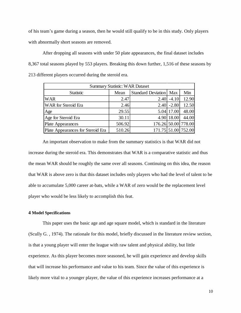
After dropping all seasons with under 50 plate appearances, the final dataset includes

8,367 total seasons played by 553 players. Breaking this down further, 1,516 of these seasons by

213 different players occurred during the steroid era.

An important observation to make from the summary statistics is that WAR did not

increase during the steroid era. This demonstrates that WAR is a comparative statistic and thus

the mean WAR should be roughly the same over all seasons. Continuing on this idea, the reason

that WAR is above zero is that this dataset includes only players who had the level of talent to be

able to accumulate 5,000 career at-bats, while a WAR of zero would be the replacement level

player who would be less likely to accomplish this feat.

4 Model Specifications

This paper uses the basic age and age square model, which is standard in the literature

(Scully G. , 1974). The rationale for this model, briefly discussed in the literature review section,

is that a young player will enter the league with raw talent and physical ability, but little

experience. As this player becomes more seasoned, he will gain experience and develop skills

that will increase his performance and value to his team. Since the value of this experience is

likely more vital to a younger player, the value of this experience increases performance at a

Statistic Mean Standard Deviation Max Min

WAR 2.47 2.40 -4.10 12.90

WAR for Steroid Era 2.46 2.40 -2.80 12.50

Age 29.55 5.04 17.00 48.00

Age for Steroid Era 30.11 4.90 18.00 44.00

Plate Appearances 506.92 176.26 50.00 778.00

Plate Appearances for Steroid Era 510.26 171.75 51.00 752.00

Summary Statistic: WAR Dataset

11

diminishing rate. Furthermore, a player’s physical ability will increase more rapidly at the

beginning of his career before he arrives at the peak of his athletic maturity. His physical ability

will then begin to deteriorate at some point due to the rigors of Major League Baseball’s 160

game season, resulting in the player’s career beginning to experience a decline in performance.

This will likely happen at an increasing rate resulting in a player’s performance declining by a

greater amount each season. This study chose to look at age versus the other measures discussed

in the literature review (career plate appearances, years since first season, and seasons) since the

impact of steroid will likely impact age specifically as the drugs will allow older player to

recover more quickly and maintain peak athletic conditions at an older age.

Next, to deal with the steroid era portion of the model, the paper uses a dummy variable

for any season that was played by a player from 1994 to 2004, which is generally considered the

steroid era by the literature (Fair, 2008)12

. Since this paper’s goal is not to address whether or not

players used steroids, but to investigate whether aging during this period was different as

individual-level data on which specific players’ actually used of steroids is not an issue.

The model also includes a few variables to control for disparity that might impact player

performance. The most important variable was a dummy for whether the designated hitter rule

was in effect.13

This rule would likely decrease player’s WAR as managers might use the

designated hitter position for full time players that are too old to play in the field anymore, but

still might be an asset to the team with their bat. This would have a negative impact on WAR

first because, these players would not accumulate defensive statistics and since designated hitters

take a large negative replacement value. Since the designated hitter rule only impacts player in

12

The first official steroid testing in Major League Baseball with players names released for failed tests was

implemented before the 2005 season (Special Report: Drug Policy in Baseball, 2008). 13

Beginning in 1973, the American League implemented a rule that a player who was not playing another position

could bat for the pitcher.

12

the American League and not the National League, this model includes a dummy variable for if a

season was played for an American League team as well as an interaction term between this

American League dummy and the designated hitter dummy.

The last variable which was included was a dummy of whether the season happened

before the pitcher’s mound was lowered in 1969 after the “year of the pitcher.”14

By including

this dummy, we can remove any impact that playing with the higher mound and non-

standardized mound height might have had an impact on player performance both offensively as

well as defensively.

Finally, to estimate the coefficients, a panel regression model was used. In this model

player fixed-effects were used in order to remove the difference in talent level between players.

In contrast, this model does not use year fixed-effects due to the fact that this would remove

much of the variation that this paper is looking for between the years in the steroid era and all

other times in baseball history. Additionally, since age increases by one with each year, there is a

massive amount of correlation between age and any type of linear year model.

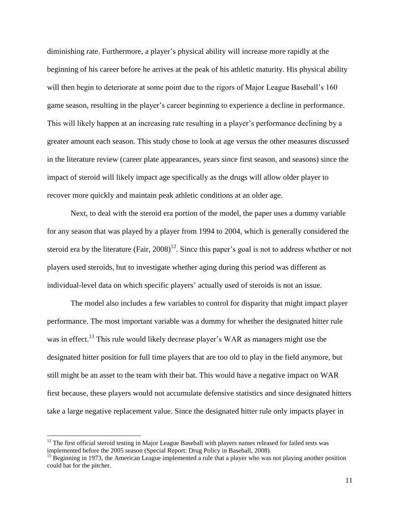
The main model is:

14

In 1968, hitters had one of the worst years in history. As a result of his fear that fans might lose interest in the

game, the commissioner of Major League Baseball created a rule that standardized the higher of the pitcher’s mound

as well as lowered the mound (Leggett, 1969).

13

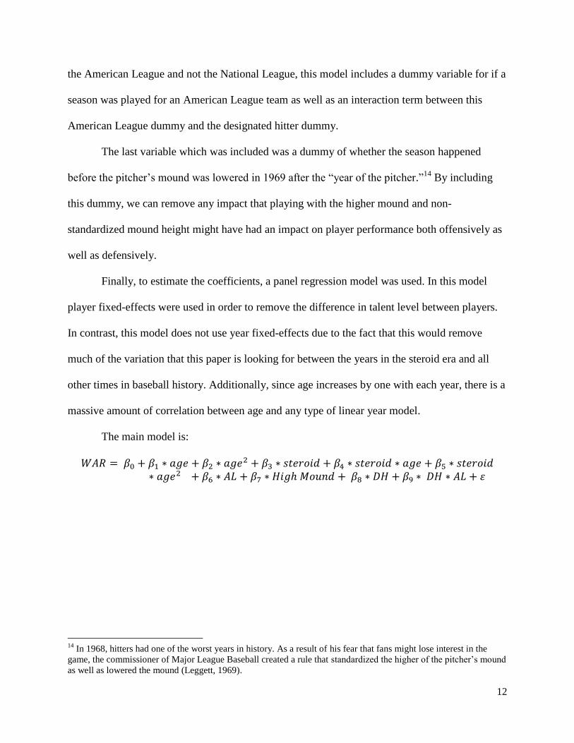
4.1 Regression Results

The first result of the regression (see Regression Table 1 below) was that the same basic

age and age squared relationship from other literature (Scully G. , 1974) was significant at a 1%

confidence level for all four of the models. This fact along with further tests discussed in the

robustness checking section demonstrates that the impact of age on Wins above Replacement

follows this form.

Moving onto our most important results, the steroid terms are all significant when they

are added to the model. An interesting aspect of these results is the fact that just including a

dummy for the steroid era, as seen in Model 2, is only significant at a 10% confidence level,

REGRESSION TABLE 1: Impact of Age on WAR

(1) (2) (3) (4)

war war war war

Age 1.516*** 1.515*** 1.512*** 1.435***

[0.045] [0.045] [0.045] [0.050]

Age Squared -0.027*** -0.027*** -0.027*** -0.026***

[0.001] [0.001] [0.001] [0.001]

Steroid 0.134* -1.403*** -8.342***

[0.069] [0.413] [1.997]

Steroid*Age 0.051*** 0.520***

[0.013] [0.133]

Steroid*Age Squared -0.008***

[0.002]

American League 0.363*** 0.363*** 0.367*** 0.359***

[0.130] [0.130] [0.130] [0.130]

DHrule -0.172 -0.169 -0.106 -0.100

[0.133] [0.133] [0.134] [0.133]

AL*DHrule -0.532*** -0.533*** -0.538*** -0.540***

[0.143] [0.143] [0.143] [0.143]

highMound 0.046 0.043 -0.008 -0.023

[0.127] [0.126] [0.127] [0.127]

_cons -17.883*** -17.875*** -17.713*** -16.590***

[0.673] [0.672] [0.673] [0.743]

N 8367 8367 8367 8367

R^2: within 0.2053 0.2057 0.2071 0.2084

R^2: between 0.0062 0.007 0.0107 0.013

R^2: overall 0.0963 0.0969 0.0976 0.0979

Notes: The model is a panel regression models. The dependent variable is WAR, wins above

replacement. Player fixed effects have been added to all specificitons. Standard errors are in

brackets. * denotes significance at a 10%, ** at 5% and *** at 1%.

14

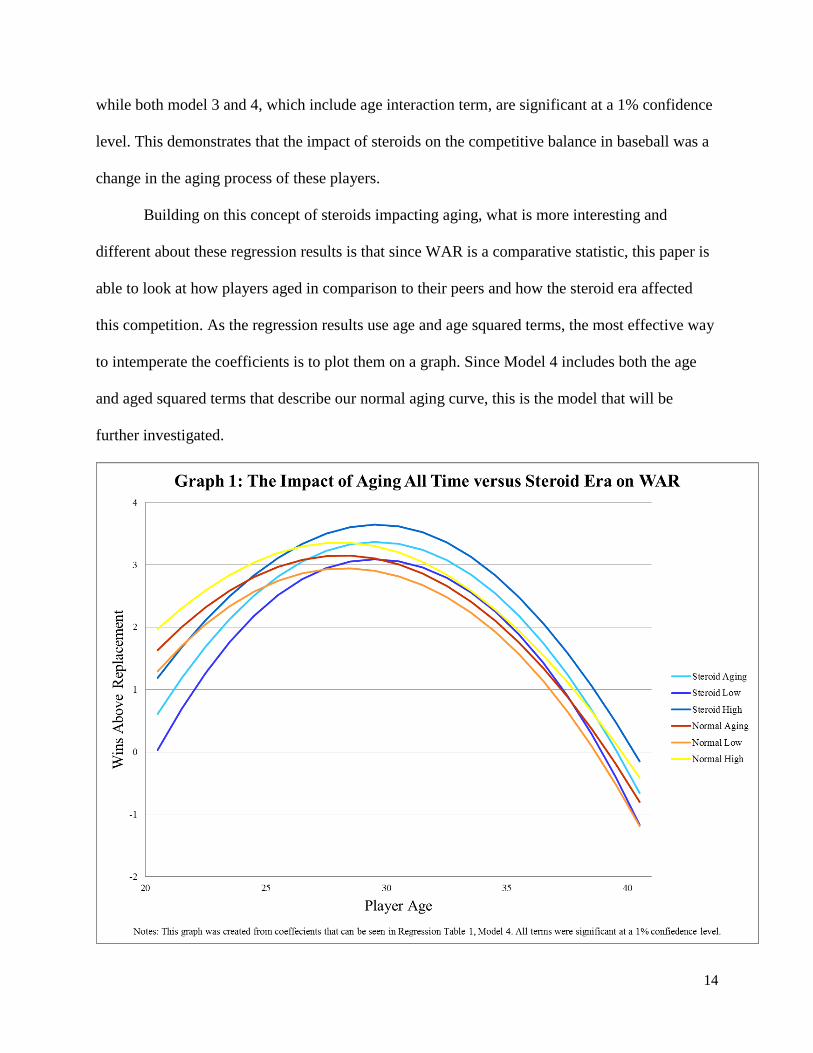
while both model 3 and 4, which include age interaction term, are significant at a 1% confidence

level. This demonstrates that the impact of steroids on the competitive balance in baseball was a

change in the aging process of these players.

Building on this concept of steroids impacting aging, what is more interesting and

different about these regression results is that since WAR is a comparative statistic, this paper is

able to look at how players aged in comparison to their peers and how the steroid era affected

this competition. As the regression results use age and age squared terms, the most effective way

to intemperate the coefficients is to plot them on a graph. Since Model 4 includes both the age

and aged squared terms that describe our normal aging curve, this is the model that will be

further investigated.

15

The most striking result from the graph (see Graph 1) is the fact that the peak age of

players shifted to the right during the steroid era, or players reached their peak at an older age

during this time period. To quantify this, during the steroid era players reached their peak at an

average age of 29.057 versus 27.655 for all other years, these ages are statistically different at a 1%

confidence level. 15

In addition, the players seem to be able to reach a higher peak on average

than they were able to reach a higher number of wins above replacement at this peak than before

the steroid era.

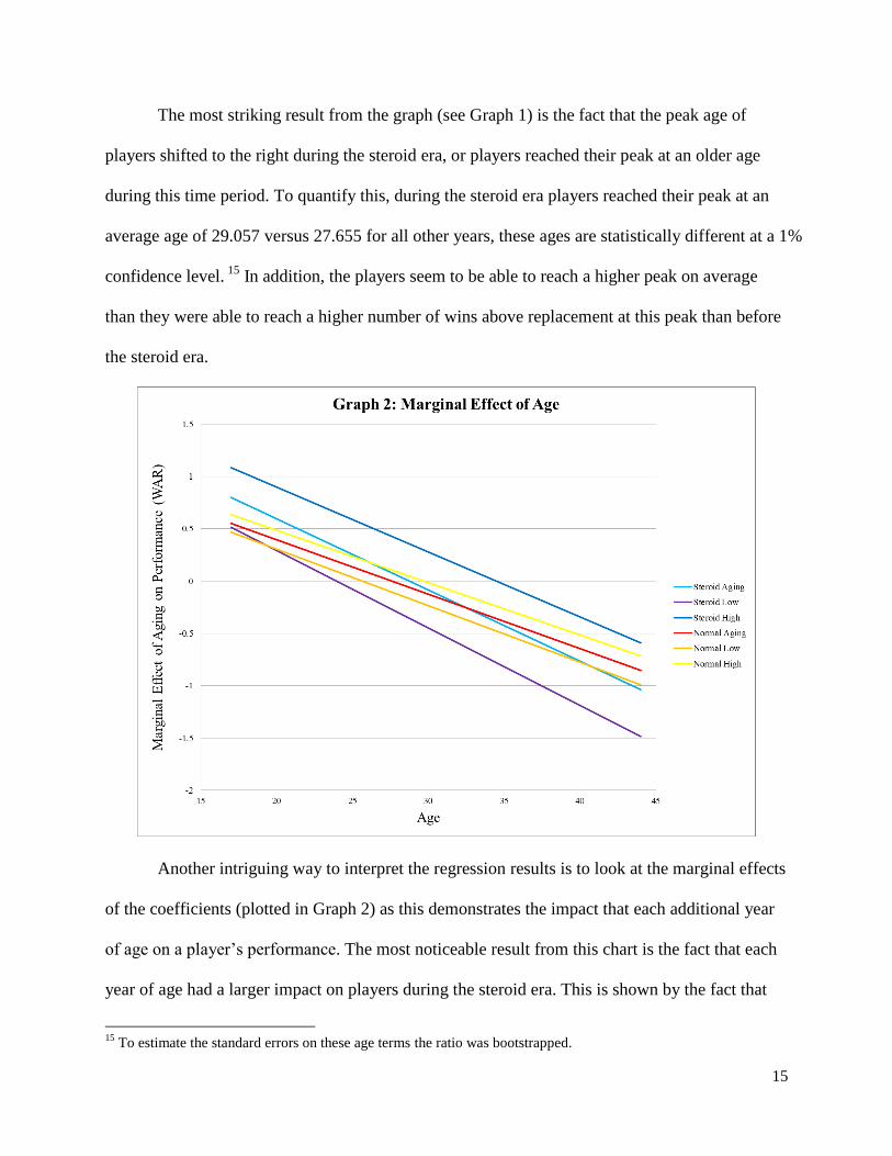
Another intriguing way to interpret the regression results is to look at the marginal effects

of the coefficients (plotted in Graph 2) as this demonstrates the impact that each additional year

of age on a player’s performance. The most noticeable result from this chart is the fact that each

year of age had a larger impact on players during the steroid era. This is shown by the fact that

15

To estimate the standard errors on these age terms the ratio was bootstrapped.

16

the marginal effects of aging has larger slope during the steroid era. This means that the aging

process during the steroid era was more drastic than any other time in baseball history.

To expand on this idea, for older player, this means that the impact of aging on their

performance was more dramatic, which is in agreement with most literature on the negative

effects of steroids (Manning, 2002). In general, the use of steroids in excess leads to such large

muscles that extra stress being placed on joints. As a result, there is an increase in joint and

ligament injuries (Manning, 2002). Dr. James Andrew of Birmingham, Alabama who is

considered to be one of the top sports medicine professionals in the world said in the article

discussed in the literature review, “We see four to five times increased incidence in tendon and

muscle ruptures in my practice compared to what we saw 10 years ago (note this quote is from

2002)… Not only do they pull them, but they tear them in two.”

17

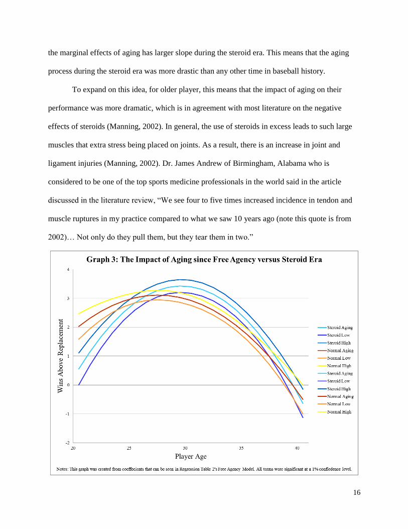
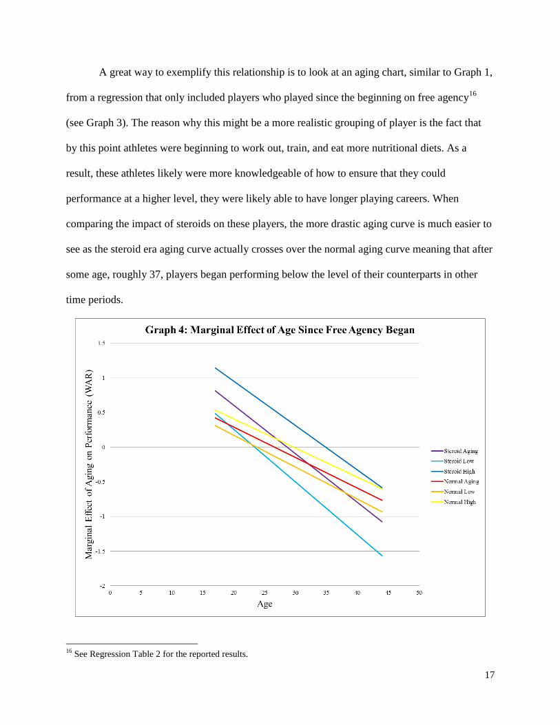
A great way to exemplify this relationship is to look at an aging chart, similar to Graph 1,

from a regression that only included players who played since the beginning on free agency16

(see Graph 3). The reason why this might be a more realistic grouping of player is the fact that

by this point athletes were beginning to work out, train, and eat more nutritional diets. As a

result, these athletes likely were more knowledgeable of how to ensure that they could

performance at a higher level, they were likely able to have longer playing careers. When

comparing the impact of steroids on these players, the more drastic aging curve is much easier to

see as the steroid era aging curve actually crosses over the normal aging curve meaning that after

some age, roughly 37, players began performing below the level of their counterparts in other

time periods.

16

See Regression Table 2 for the reported results.

18

An intriguing consequence of the steroid era is that players began their careers at a lower

level than other time periods. To begin with, by this point in time the number of teenage Major

League Baseball players was much smaller than in the earlier years of baseball and thus it would

make sense that the average player during this time period would be below the replacement level

before the age of 20. In addition, the steroid era allowed the elite players from the generation

before to be able to perform at a higher level than any other time in baseball history and they

were able to do this at an older age than ever before. Since WAR is a comparative statistic, the

fact that the last generation was still able to play at a higher level for a longer period of time

means that these younger players would likely need to wait longer for the opportunity to play and

once they received this opportunity, they would likely initially perform at comparatively a lower

level. Adding to this idea is that players who did use steroid for a longer period of time would

likely be able to build up their strength to a point where they would have a competitive

advantage over the younger players. To build on this concept, the minor leagues implemented a

steroid testing policy much earlier than the major leagues (Schmidt, 2010). Thus, these younger

players would be less likely to be on steroids and if they were then they would have been on

them for a shorter period of time.

Finally, to review the control in the model, the designated hitter rule dummy comes out

insignificant in all of the models, but the designated hitter interaction term with American

League comes out negatively significant. This is in agreement with the idea that was expressed in

the model specification portion that the designated hitter rule would have little impact on the

players in the National League. In addition, the negative coefficient is also in agreement with the

paper’s prediction because position would potentially decrease WAR as the player who plays

19

this position would have a very low replacement level, would not accumulate defensive statistics,

and in most cases an older slugger at the end of his career, thus likely close to replacement level.

4.2 Robustness Checking

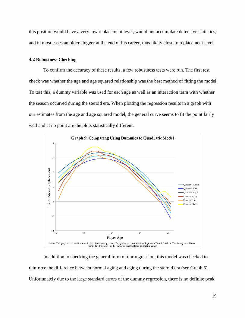
To confirm the accuracy of these results, a few robustness tests were run. The first test

check was whether the age and age squared relationship was the best method of fitting the model.

To test this, a dummy variable was used for each age as well as an interaction term with whether

the season occurred during the steroid era. When plotting the regression results in a graph with

our estimates from the age and age squared model, the general curve seems to fit the point fairly

well and at no point are the plots statistically different.

In addition to checking the general form of our regression, this model was checked to

reinforce the difference between normal aging and aging during the steroid era (see Graph 6).

Unfortunately due to the large standard errors of the dummy regression, there is no definite peak

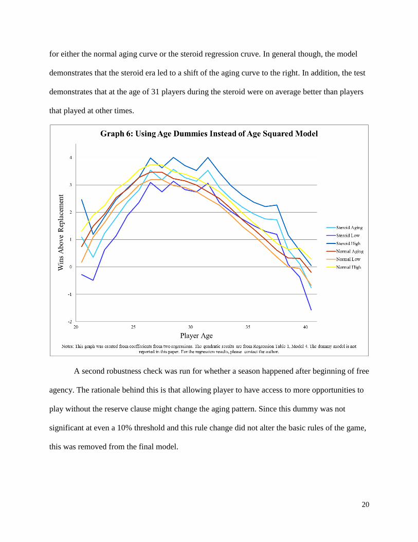
20

for either the normal aging curve or the steroid regression cruve. In general though, the model

demonstrates that the steroid era led to a shift of the aging curve to the right. In addition, the test

demonstrates that at the age of 31 players during the steroid were on average better than players

that played at other times.

A second robustness check was run for whether a season happened after beginning of free

agency. The rationale behind this is that allowing player to have access to more opportunities to

play without the reserve clause might change the aging pattern. Since this dummy was not

significant at even a 10% threshold and this rule change did not alter the basic rules of the game,

this was removed from the final model.

21

The third major issue brought up after the potential issue of free agency or looking just at

the modern area was the fact that with the advent of the designated hitter rule in baseball, teams

were able to play an older player at this position without having to worry about the player’s

defensive ability. Unfortunately, due to the fact that these players potentially might not have

been able to continue to play if there was no designated hitter rule, this could lead to some bias

issues. To test this, the study ran the main regression dropping all 383 season played by a

designated hitter. When season of designated hitters was dropped, the results did not change (see

Regression Table 2) demonstrating that a bias of older player playing designated hitters is not a

bias driving our results.

REGRESSION TABLE 2: Impact of Age on WAR Robustness Checking

All Free Agency No DH No Combined No Bonds

war war war war war

age 1.435*** 1.170*** 1.446*** 1.497*** 1.428***

[0.050] [0.078] [0.092] [0.086] [0.050]

agesq -0.026*** -0.022*** -0.026*** -0.027*** -0.026***

[0.001] [0.001] [0.002] [0.001] [0.001]

steroid -8.342*** -13.030*** -9.769*** -7.966*** -8.697***

[1.997] [2.249] [2.493] [2.456] [1.994]

steroidage 0.520*** 0.834*** 0.620*** 0.498*** 0.546***

[0.133] [0.149] [0.167] [0.164] [0.133]

steroidAgesq -0.008*** -0.013*** -0.009*** -0.007*** -0.008***

[0.002] [0.002] [0.003] [0.003] [0.002]

AL 0.359*** -0.179** 0.324* 0.359* 0.359***

[0.130] [0.083] [0.185] [0.195] [0.129]

DHrule -0.100 - -0.110 -0.081 -0.095

[0.133] - [0.171] [0.176] [0.133]

ALDHrule -0.540*** - -0.382* -0.560*** -0.540***

[0.143] - [0.198] [0.207] [0.142]

highMound -0.023 - -0.042 -0.019 -0.027

[0.127] - [0.173] [0.174] [0.127]

_cons -16.590*** -12.735*** -16.794*** -17.512*** -16.503***

[0.743] [1.177] [1.328] [1.242] [0.743]

N 8367 4718 7984 7896 8345

R^2: within 0.2084 0.2079 0.2079 0.2026 0.2091

R^2: between 0.013 0.0363 0.0363 0.0105 0.0111

R^2: overall 0.0979 0.1068 0.1068 0.0957 0.1013

Notes: The model is a cross-sectional time-series regression models. Standard errors are in

brackets. * denotes significance at a 10%, ** at 5% and *** at 1%.

22

A further potentially issue that was tested was the fact that players who were trading took

a one for the value of their American League Dummy if they began their season in the American

League. Since 471 of the 8367 seasons played included trades and whether a player changed

league during the trade was not recorded, these 471 seasons were removed to test if they were

affect the results. Since these results do not change the impact of aging on player performance,

the final regression included these seasons.

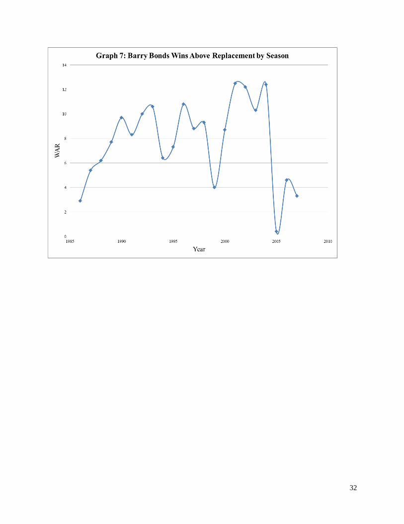
Yet another test was removing just Barry Bonds from this dataset because his late career

performance is consider an extreme outlier (see Graph 7 in Tables and Figures) and is a major

point of discussion in the literature (Tobin, 2007). As soon in the motivation portion of this paper,

Barry Bonds had three of the best seasons in Major League History at an age six year older than

any other player in the top fifteen. Interesting the next best season for a player over the age of

thirty-five is the twenty-ninth best season ever played at the age of thirty-eight by Barry Bonds

himself. It takes until the fifty-eigth best season ever by Ted Williams at the age of thirty-eight

for any other player to have a season of this caliber after thirty-five. In this check, the results did

not differ significantly from the main model (see Regression Table 2).

An additional test was using a dummy variable for the various ways which Total Zone17

is calculated was also tested, since the method has changed over time as the amount of

information on play by play recording of baseball games has varied. This was done due to

possibility that using a different measure of Total Zone might systematically change the

defensive portion the WAR statistic. However, when testing this variable, it was only significant

17

Total Zone is a method for measuring a player’s defensive contribution to their team. This method calculates a

league averages of the percent of the time that a ball is fielded if hit in a specific direction and then compare this to

an individual players percentage fielded. If a player’s fields a greater percentage than the league average, then they

are consider an above average fielder.

23

for offensive WAR and not defensive WAR. As a result, this likely is picking up something

besides the changes in Total Zone and as a result this was not included in the final model.

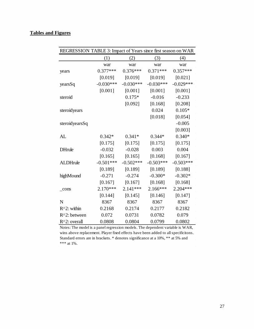
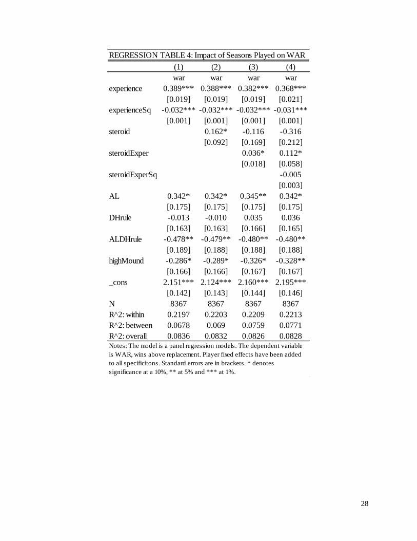
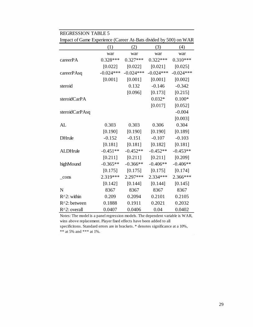
Finally, to test other methods of approaching the issue of aging, this study also tested

years of experience, years since first season, and career at-bats because both Sommers (August

2008) and Bradbury (2011) suggested that the aging process for Major League Player is

potentially better modeled using another measure than just player age. All of these different

models of the aging process similarly showed the same type of aging process as our basic age

and age squared model, but they only showed the impact of the steroid era at a 10% significance

level (see regression tables 3-5 in Tables and Figures). Even so, the significant term was an

increase in player performance as the player gained experience, demonstrating the initial increase

in performance due to steroids. Since these models do not show the same level of significance as

the age model, the age model was used for the main regression. Additionally, since only the age

model showed the relationship with steroids changing over time, this study concludes that the

effect of steroids is directly related to the age of a player versus their playing time. This is

important since it points to the steroid era’s damatise specifically the aging process of players.

5 Conclusions

This paper demonstrates that players aged differently during the steroid era than in any

time period beforehand. Importantly, the impact of the steroid era follows the basic expectations

from the literature on the subject, since players reach higher levels during the peak of their

career, but their ability diminishes at a faster rate during this period. Unfortunately, since there is

no comprehensive individual-level dataset on which players used steroids, this paper cannot

prove whether this impact is due to steroids or something else about the era.

24

Further work that can be done on this area could focus on how aging effects positions

differently and how the steroid era specifically impacted aging at these different positions. In

addition, testing semi-parametric models, which would not require any specific form could help

address any further question of whether the general age and age squared model is the proper

specification for aging in baseball.

Most importantly, one specific area which would benefit from further investigation would

be how players are aging in the current or post-steroid era. Unfortunately this cannot be done for

at least a few more seasons due to the requirements of this data set, 5,000 career at-bats. Since

this number means a player must have played in roughly 10 seasons of major league baseball, the

post-steroid era section of our dataset is currently filled only with players who are older, and

using such a dataset would lead to selection bias issues.

This further work is especially important so that Major League Baseball team’s

management can properly identify how aging is currently affecting player as well as how aging

impact players at different positions. This is important due to the size of the investment that

teams will be making in large free agent signings. As studies continued to be conducted, teams

will be able to make more accurate predictions of the level of performance they will get from

their star free agent signings.

25

Works Cited 1956, M. d. (2008, January 10). Sean Smith .

Advances in the economics of sport. (1992). Greenwich, Conn.: JAI Press.

2008, A. F. (2008). An Economic Analysis of the Effects of Steroids on Season Best Performances in

Track and Field. Retrieved March 9, 2012, from http://digitalcommons.iwu.edu/econ_honproj/86.

Alexander M Petersen, W.-S. J. (2008). On the Distrubution of Career Longevity and the Evolution of

home-run prowess in Professional Baseball. A Letters Journal Exploring the Frontiers of Physics.

Berna Demiralp, C. C. (2010). The effects of age, experience and managers upon baseball performance.

Springer Science+Business Media, LLC.

Bradbury, J. (2007). The Baseball Economist: The Real Game Exposed. New York, N.Y.: Dutton.

Bradbury, J. (2011). Hot stove economics : understanding baseball's second season. Copernicus Books:

New York.

Bradbury, J. (January 11, 2010). How Do Baseball Players Age? Investiageting the Age-27 Theory.

http://www.baseballprospectus.com/article.php?articleid=9933.

Brian J Schmotzer, J. S. (July 2008). Did Steroid Use Enhance the Performance of the Mitchell Batters?

The Effect of Alleged Performance Enhancing Drug Use on Offensive Performance from 1995 to

2007. Journal of Quantitative Analysis in Sports, Volume 4, Issue 3, Pages 1–14.

Butenko, S., Gil-Lafuente, J., & Pardalos, P. M. (2010). Optimal Strategies in Sports Economics and

Management. New York: Heidelberg: Springer.

Carter, D. M. (2011). Money games : profiting from the convergence of sports and entertainment.

Stanford, Calif.: Stanford Business Books.

Cockcroft, T. H. (February 23, 2009). Getting Beyond the “Steriod Era”. ESPN.com,

http://sports.espn.go.com/fantasy/baseball/flb/story?page=mlbdk2k9steroids.

Evans-Brown, J. M. (March 2009). Anabolic Steroids. Retrieved March 9, 2012, from

http://www.smmgp.org.uk/download/others/other055.pdf.

Fair, R. C. (2008, October). Estimated Age Effects in Baseball. Journal of Quantitative Analysis in

Sports, Vol. 4: Iss. 1, Article 1.

Fizel, J. (2006). Handbook of Sports Economics Research. Armonk, N.Y.: M.E. Sharpe.

Fort, R. D. (2006). Sports economics . Upper Saddle River, N.J.: Pearson Prentice Hall.

Gennaro, V. (2007). Diamond dollars : the economics of winning in baseball. Hingham, MA: Maple

Street Press.

Hakes, C. T. (2007). Pay, productivity and aging in Major League Baseball. Munich Personal RePEc

Archive, http://mpra.ub.uni-muenchen.de/4326/1/MPRA_paper_4326.pdf.

Jane, W.-J. (2010). Raising Salary or redistributing it: A Panel Analysis of Major League Baseball.

Economics Letters, pp. 297-99.

Jazayerli, R. (October 13, 2011). Doctoring the Numbers, Starting them Young Part 1 .

http://www.baseballprospectus.com/article.php?articleid=15295.

Jewell, R. T., McPherson, M. A., & Molina, D. J. (2004). Testing the Determinants of Income

Distribution in Major League Baseball. Economic Inquiry, 469-482.

John Fizel, E. G. (1999). Sports economics : current research. Westport, Conn.: Praeger.

Katie Stankiewicz, '. (2009). Length of Contracts and the Effect on the Performance of MLB Players.

Honors Projects, http://digitalcommons.iwu.edu/econ_honproj/103.

Lewis, R. F. (2010). Smart ball : marketing the myth and managing the reality of major league baseball.

Jackson, Mississippi: University Press of Mississippi.

Lichtman, M. (December 21, 2009). How do Baseball Players Age? (Part 1).

http://www.hardballtimes.com/main/article/how-do-baseball-players-age-part-1/.

Manning, A. (2002, July 8). Build Muscles, Shrinks Careers. USA Today, p. 3C.

Mark J. Eschenfelder, M. L. (2007). Economics of sport. Morgantown, WV: Fitness Information

Technology.

26

Mitchell Grossman, T. K. (n.d.). Steroids and Major League Baseball. Retrieved March 9, 2012, from

http://faculty.haas.berkeley.edu/rjmorgan/mba211/steroids%20and%20major%20league%20base

ball.pdf

Onge, J. M., Rogers, R. G., & Krueger, P. M. (2008). Major League Baseball Players' Life Expectancies.

Social Science Quarterly, 817-830.

Osborne, E. (2005, June). Performance-Enhancing Drugs: An Economic Analysis. Retrieved March 9,

2012, from www.wright.edu/~eosborne/research/steroids.doc.

Osbrone, E. (2005). Performance-Enhancing Dugs: An Economics Analysis. ?

Pelton, K. (2010, February 2). Rethinking NBA Aging: Chaos or order?

http://basketballprospectus.com/article.php?articleid=896.

Rockerbie, D. W. (June 2009). Strategic Free Agency in Baseball. Journal of Sports Economics, pp. 278-

91.

Scully, G. (1974). Pay Performance and Major League Baseball. The American Economic Review, 915-

930.

Scully, G. W. (1995). The market structure of sports. Chicago, IL: University of Chicago Press.

Smith, S. (2008 , March 25). Measuring defense for players back to 1956 (Part 2).

http://www.hardballtimes.com/main/article/measuring-defense-for-players-back-to-1956-part-2/.

Sommers, P. (August 2008). The Changing Hitting Performance in Major League Baseball,1966-2006.

Journal of Sports Economics, v. 9, iss. 4, pp. 435-40.

Sommers, P. M. (1992). Diamonds are forever: The business of baseball. Washington, D.C.: Brookings

Institution.

Surdam, D. G. (2010). The ball game biz : an introduction to the economics of professional team sports.

Jefferson, N.C.: McFarland & Co.

Thurston, J. (1990). Chemical Warfare: Battling Steroids in Athletics. Marquette Sports Law Review.

Tobin, R. G. (2007, August). On the Potential of Chemical Bonds: Possible Effects of Steroids on Home

Run Production in Baseball. Retrieved March 9, 2012, from

http://scitation.aip.org/journals/doc/AJPIAS-ft/vol_76/iss_1/15_1.html.

Vany, A. D. (2010). Steroids and Home Runs. Retrieved March 9, 2012, from

www.arthurdevany.com/downloads/20100226/download

Winfree, J. D. (2007, August 23). The Law of Genius and Home Runs Refuted. Retrieved March 9, 2012,

from http://www-personal.umich.edu/~jdinardo/lawsofgenius.pdf

27

Tables and Figures

REGRESSION TABLE 3: Impact of Years since first season on WAR

(1) (2) (3) (4)

war war war war

years 0.377*** 0.376*** 0.371*** 0.357***

[0.019] [0.019] [0.019] [0.021]

yearsSq -0.030*** -0.030*** -0.030*** -0.029***

[0.001] [0.001] [0.001] [0.001]

steroid 0.175* -0.016 -0.233

[0.092] [0.168] [0.208]

steroidyears 0.024 0.105*

[0.018] [0.054]

steroidyearsSq -0.005

[0.003]

AL 0.342* 0.341* 0.344* 0.340*

[0.175] [0.175] [0.175] [0.175]

DHrule -0.032 -0.028 0.003 0.004

[0.165] [0.165] [0.168] [0.167]

ALDHrule -0.501*** -0.502*** -0.503*** -0.503***

[0.189] [0.189] [0.189] [0.188]

highMound -0.271 -0.274 -0.300* -0.302*

[0.167] [0.167] [0.168] [0.168]

_cons 2.170*** 2.141*** 2.166*** 2.204***

[0.144] [0.145] [0.146] [0.147]

N 8367 8367 8367 8367

R^2: within 0.2168 0.2174 0.2177 0.2182

R^2: between 0.072 0.0731 0.0782 0.079

R^2: overall 0.0808 0.0804 0.0799 0.0802Notes: The model is a panel regression models. The dependent variable is WAR,

wins above replacement. Player fixed effects have been added to all specificitons.

Standard errors are in brackets. * denotes significance at a 10%, ** at 5% and

*** at 1%.

28

REGRESSION TABLE 4: Impact of Seasons Played on WAR

(1) (2) (3) (4)

war war war war

experience 0.389*** 0.388*** 0.382*** 0.368***

[0.019] [0.019] [0.019] [0.021]

experienceSq -0.032*** -0.032*** -0.032*** -0.031***

[0.001] [0.001] [0.001] [0.001]

steroid 0.162* -0.116 -0.316

[0.092] [0.169] [0.212]

steroidExper 0.036* 0.112*

[0.018] [0.058]

steroidExperSq -0.005

[0.003]

AL 0.342* 0.342* 0.345** 0.342*

[0.175] [0.175] [0.175] [0.175]

DHrule -0.013 -0.010 0.035 0.036

[0.163] [0.163] [0.166] [0.165]

ALDHrule -0.478** -0.479** -0.480** -0.480**

[0.189] [0.188] [0.188] [0.188]

highMound -0.286* -0.289* -0.326* -0.328**

[0.166] [0.166] [0.167] [0.167]

_cons 2.151*** 2.124*** 2.160*** 2.195***

[0.142] [0.143] [0.144] [0.146]

N 8367 8367 8367 8367

R^2: within 0.2197 0.2203 0.2209 0.2213

R^2: between 0.0678 0.069 0.0759 0.0771

R^2: overall 0.0836 0.0832 0.0826 0.0828Notes: The model is a panel regression models. The dependent variable

is WAR, wins above replacement. Player fixed effects have been added

to all specificitons. Standard errors are in brackets. * denotes

significance at a 10%, ** at 5% and *** at 1%.

29

REGRESSION TABLE 5

Impact of Game Experience (Career At-Bats divided by 500) on WAR

(1) (2) (3) (4)

war war war war

careerPA 0.328*** 0.327*** 0.322*** 0.310***

[0.022] [0.022] [0.021] [0.025]

careerPAsq -0.024*** -0.024*** -0.024*** -0.024***

[0.001] [0.001] [0.001] [0.002]

steroid 0.132 -0.146 -0.342

[0.096] [0.173] [0.215]

steroidCarPA 0.032* 0.100*

[0.017] [0.052]

steroidCarPAsq -0.004

[0.003]

AL 0.303 0.303 0.306 0.304

[0.190] [0.190] [0.190] [0.189]

DHrule -0.152 -0.151 -0.107 -0.103

[0.181] [0.181] [0.182] [0.181]

ALDHrule -0.451** -0.452** -0.452** -0.453**

[0.211] [0.211] [0.211] [0.209]

highMound -0.365** -0.366** -0.406** -0.406**

[0.175] [0.175] [0.175] [0.174]

_cons 2.319*** 2.297*** 2.334*** 2.366***

[0.142] [0.144] [0.144] [0.145]

N 8367 8367 8367 8367

R^2: within 0.209 0.2094 0.2101 0.2105

R^2: between 0.1888 0.1911 0.2021 0.2032

R^2: overall 0.0407 0.0406 0.04 0.0402

Notes: The model is a panel regression models. The dependent variable is WAR,

wins above replacement. Player fixed effects have been added to all

specificitons. Standard errors are in brackets. * denotes significance at a 10%,

** at 5% and *** at 1%.

30

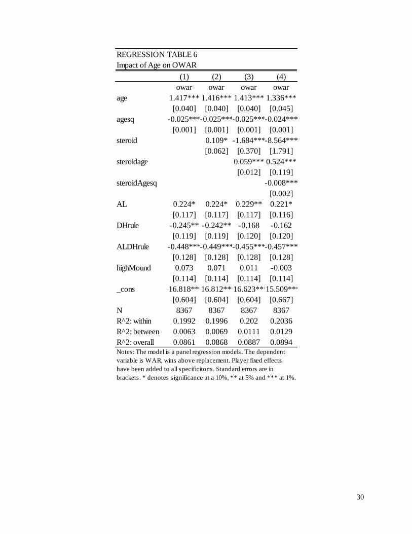
REGRESSION TABLE 6

Impact of Age on OWAR

(1) (2) (3) (4)

owar owar owar owar

age 1.417*** 1.416*** 1.413*** 1.336***

[0.040] [0.040] [0.040] [0.045]

agesq -0.025***-0.025***-0.025***-0.024***

[0.001] [0.001] [0.001] [0.001]

steroid 0.109* -1.684***-8.564***

[0.062] [0.370] [1.791]

steroidage 0.059*** 0.524***

[0.012] [0.119]

steroidAgesq -0.008***

[0.002]

AL 0.224* 0.224* 0.229** 0.221*

[0.117] [0.117] [0.117] [0.116]

DHrule -0.245** -0.242** -0.168 -0.162

[0.119] [0.119] [0.120] [0.120]

ALDHrule -0.448***-0.449***-0.455***-0.457***

[0.128] [0.128] [0.128] [0.128]

highMound 0.073 0.071 0.011 -0.003

[0.114] [0.114] [0.114] [0.114]

_cons -16.818***-16.812***-16.623***-15.509***

[0.604] [0.604] [0.604] [0.667]

N 8367 8367 8367 8367

R^2: within 0.1992 0.1996 0.202 0.2036

R^2: between 0.0063 0.0069 0.0111 0.0129

R^2: overall 0.0861 0.0868 0.0887 0.0894Notes: The model is a panel regression models. The dependent

variable is WAR, wins above replacement. Player fixed effects

have been added to all specificitons. Standard errors are in

brackets. * denotes significance at a 10%, ** at 5% and *** at 1%.

31

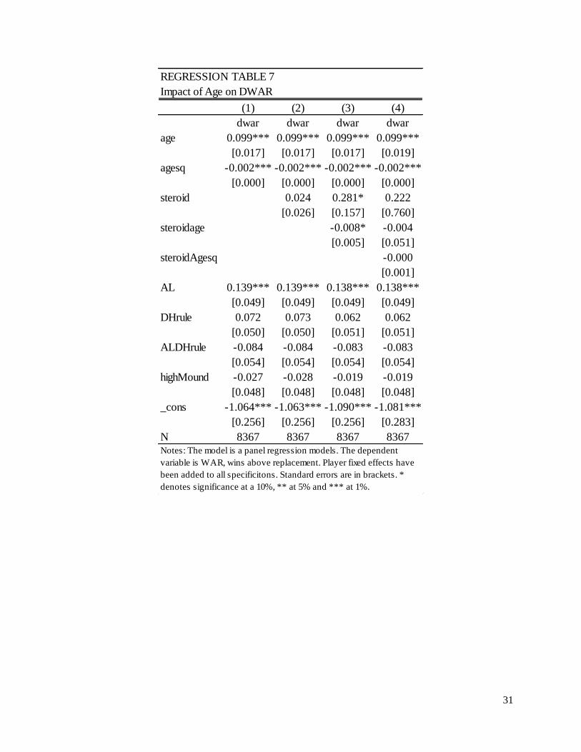
REGRESSION TABLE 7

Impact of Age on DWAR

(1) (2) (3) (4)

dwar dwar dwar dwar

age 0.099*** 0.099*** 0.099*** 0.099***

[0.017] [0.017] [0.017] [0.019]

agesq -0.002*** -0.002*** -0.002*** -0.002***

[0.000] [0.000] [0.000] [0.000]

steroid 0.024 0.281* 0.222

[0.026] [0.157] [0.760]

steroidage -0.008* -0.004

[0.005] [0.051]

steroidAgesq -0.000

[0.001]

AL 0.139*** 0.139*** 0.138*** 0.138***

[0.049] [0.049] [0.049] [0.049]

DHrule 0.072 0.073 0.062 0.062

[0.050] [0.050] [0.051] [0.051]

ALDHrule -0.084 -0.084 -0.083 -0.083

[0.054] [0.054] [0.054] [0.054]

highMound -0.027 -0.028 -0.019 -0.019

[0.048] [0.048] [0.048] [0.048]

_cons -1.064*** -1.063*** -1.090*** -1.081***

[0.256] [0.256] [0.256] [0.283]

N 8367 8367 8367 8367Notes: The model is a panel regression models. The dependent

variable is WAR, wins above replacement. Player fixed effects have

been added to all specificitons. Standard errors are in brackets. *

denotes significance at a 10%, ** at 5% and *** at 1%.

32