1

Estimating the Value of Major League Baseball Players

Brian Fields* East Carolina University

Department of Economics Masters Paper July 26, 2001

Abstract

This paper examines whether Major League Baseball players are paid their marginal revenue product. A two-step estimation technique is used with data from 1990 to 1999. First, I estimate a regression relating team revenues to the team’s winning percentage and other explanatory variables. The second regression estimates the relationship between winning percentage and team statistics. Given the estimates from these two models I can calculate player marginal revenue product by first predicting how his statistics will affect the team’s winning percentage and then relating the impact on winning percentage on team revenue. The results indicate that professional baseball players are underpaid in marginal earnings per dollar of marginal revenue product. Players were paid more of their marginal product after the 1994-95 strike and older players appear to receive a salary closer to their marginal products than younger players.

* The author would like to thank Dr. Ed Schumacher for his help and guidance in all phases of this paper

2

I. Introduction It is often debated whether or not professional baseball players are worth the large

salaries they receive. Recent deals such as Alex Rodriguez’s $125 million contract with

Texas and Manny Ramirez’s $96 million contract with Boston have caused many to

speculate that baseball players are paid more than they are worth. A recent report from

the Independent Members of the Commissioner’s Blue Ribbon Panel on Baseball

Economics concluded that from 1995-99 only three teams (Cleveland, Colorado, and

New York Yankees) achieved profitability (Levin et al. 2000). These factors have

resulted in arguments for revenue sharing, a tax on clubs with payrolls over a fixed

threshold, and other measures to attempt to lower players’ salaries.

Baseball is a game of statistics that has proven to be an interesting labor market

for economists, providing detailed measures of individual productivity. Unlike other

professions, there are lots of data on individual performance and productivity. In

addition, the fact that baseball players’ marginal revenue products are relatively

independent, makes it easier to separate a particular player’s contribution to his team

(Krautman 369). Thus, one can potentially estimate a players’ marginal revenue product

and compare it to his actual salary.

The purpose of this paper is to analyze pay-performance results of Major League

Baseball players in a refined Scully model. I follow the work of MacDonald and

Reynolds (1994) using data from 1990-1999, and examine whether professional baseball

players are paid their marginal revenue product. The paper also examines if there was a

significant change after the 1994-95 strike. The next section provides some background

on labor relations in baseball. Section III provides a literature review. The team model

3

and marginal revenue product equations are in section IV with the data, variables, and

descriptive statistics in section V. The last two sections provide the results and the

conclusion.

II. Background From 1879 to Major League Baseball’s first collective labor agreement in 1968,

various kinds of reserve clauses restricted the player’s freedom of negotiation with the

owner of the contract. The player’s baseball services were bound to one team until that

player’s rights were transferred. These contracts also were a privately and socially

efficient means to finance player development and the inevitable failure of most minor

league players to produce in the majors (MacDonald and Reynolds 1994). MacDonald

states that the usual presumption is that the reserve clause kept salaries below those that

might prevail in a more competitive environment. After 1968, compensation rules were

modified but considerable controversy existed over the economic impact of the

compensation scheme. In 1986-87, Major League Baseball players were grouped into

three contract environments: ‘rookies’ in years 1-2 subject to a team reserve clause and

ineligible for salary arbitration and free agency; intermediate players in years 3-6 eligible

for final-offer salary arbitration but not free agency; and senior players after 6 years

eligible for either final-offer salary arbitration or free agency. (MacDonald and Reynolds

1994). Free agency allows players to negotiate freely with any team.

Baseball does not have any form of salary cap, although it does have a luxury tax

on teams that annually spend beyond a certain amount on salaries. The first discussion of

salary cap in baseball negotiations occurred in 1989-90. The owners proposed a cap that

would limit the amount of salary any team could pay to players. Those with six years of

4

experience would still be free agents. However, a team would not sign them if doing so

would put the team over the salary cap. Also part of the owners’ proposal was a

guarantee to the players of 43 percent of revenue from ticket sales and broadcast

contracts, which was about 82 percent of owners’ total revenue (Staudohar 1998).

The purpose of the proposed salary cap was to protect teams in small markets

from having their talented free agents brought up by big market teams. In theory, teams

in large cities would be unable to dominate the free agent market because the cap would

limit the players they could sign. Also, because teams spend large sums in developing

young players, a salary cap would allow them to retain more of their young players

because free agency opportunities would be more limited (Staudohar 1998).

On December 31, 1993, baseball’s 4-year collective bargaining agreement

expired. Baseball, as other sports, had its big market and small-market teams and

economic disparities between clubs. Baseball teams share money from the sale of

national broadcast rights equally but kept all sales from local broadcast rights. As a

result, the owners decided to share some of their local revenues, but only if the players

accepted the salary cap. The owners also proposed to share their revenues with the

players, 50-50. Depending on the players’ share under the 50-50 split, no team could

have a payroll of more than 110 percent or less than 84 percent of the average payroll for

all teams. The Major League Baseball Players Association (MLBPA) rejected the salary

cap and other major proposals. This set the stage for a strike that began on August 12,

1994 and lasted for 232 days – the longest strike ever in professional sports. In the end

MLBPA accepted a modified version of the luxury tax. The early returns indicate that it

5

is having little if any effect on average player salaries (Staudohar 1998), although results

in this paper suggest there has been a significant effect.

III. Literature review

A number of previous studies have examined the marginal revenue product of

professional baseball players. The pioneering econometric study on pay versus

performance of Major League Baseball was provided by Scully (1974). While Scully’s

approach has undergone much scrutiny, it remains one of the primary methods of

estimating a player’s MRP. A number of studies have modified Scully’s basic model,

used more recent data, and improved estimation procedures. Scully (1974) estimates

MRP in a two equation model. The first is a team revenue function which relates team

revenues to the team win-loss record and the principal market characteristics of the area

in which the team plays. Then he estimates a production function, relating team output

and win-loss percentage to a number of team inputs. Scully’s results show that players

were paid only 10-20% of their marginal revenue product in data for the 1968-69

seasons. Scully found that the economic loss of professional baseball players under the

reserve clause is of considerable magnitude (Scully 1974).

Krautman (1999) revisits the Scully technique for estimating the MRP of

professional baseball players. Using a sample of available free agents from 1990-1993,

he attempts to show that the Scully technique is sensitive to the manner in which

marginal product is measured. The approach estimates the market return on performance

from a regression of free agent wages on performance. These market returns are then

applied to the performance of reserve-clause players, giving estimates their market

6

values. Krautman’s results indicate that the average apprentice (less than three years of

Major League experience) receives about 25% of his MRP and the typical journeyman

(more than three, but less than six, year of Major League experience) receives a salary

that is essentially commensurate with his value (Krautman 1999).

MacDonald and Reynolds (1994) examine if the new contractual system of free

agency and final-offer arbitration brought salaries into line with marginal revenue

products. Using public data for the 1986-87 seasons, they include all players, both hitters

and pitchers, who were on a major league roster as of August 31, 1986 and August 31,

1987. First, they analyze whether any economic evidence of owner collusion exist during

the 1986-87 period. Secondly, they use a systematic analysis of final-offer arbitration in

baseball – established three years before free agency – and find it has a stronger

independent effect on salaries than the much publicized free agency. Last, they test the

‘superstars’ model of Rosen (1981) and find the salaries of the very highest paid players

in Major League baseball disproportionately exceed their relative productivity advantage,

as the ‘superstars’ model predicts. They find that major league salaries do generally

coincide with the estimated marginal revenue products. Experienced players are paid in

accord with their productivity; however, young players are paid less than their marginal

revenue product, on average (MacDonald and Reynolds 1994).

Thus, the previous literature seems to agree that, on average, more experienced

players are paid a wage approximately equal to their marginal product while younger

players appear to be paid a wage significantly less than their marginal product. These

previous studies have used data from a few seasons and from the early 90’s or earlier. To

7

my knowledge, no previous studies have utilized data over multiple seasons or as recent

as the mid to late 90’s.

IV. Team Model and Marginal Revenue Product Employing one more unit of labor generates additional income for the firm

because of the added output that is produced and sold. Thus, the marginal income

generated with a unit of input is the multiplication of two quantities: the change in

physical output produced (marginal product) and the marginal revenue generated per unit

of physical output. Thus, the additional income created from hiring an additional worker

is termed the marginal revenue product (MRP). In theory, a firm would be willing to pay

a worker a wage up to his MRP. In a competitive labor market we would expect workers

to be paid a wage equal to their MRP.

The players’ marginal revenue product in baseball is the ability or performance

that he contributes to the team and the effect of that performance on team revenue (Scully

1974). This effect can be direct or indirect. Ability contributes to team performance and

victories raise gate receipts and broadcast revenues. Therefore a players’ market worth

can be defined as the amount of team revenue produced by his contribution to attracting

paying fans to see and hear the team compete (Scully 1974).

Ignoring special appeal for ‘superstars’, a player’s MRP essentially is based on

each player’s contribution to significant team performance variables, the effect of these

performance variables on winning percentage, and, in turn, the effect of winning

percentage on team revenue. I also assume that the team production function is linear

and is written as:

8

eOUTCONTNATLGERARCWINPCT ++++++= 543210 βββββα (1)

where WINPCT = percentage of games won by a team RC = Total team runs created for the season

ERA = teams earned run average per 9-inning game NATLG = 1 if team is in the National League, 0 otherwise

CONT = 1 if team finished within 5 games of first place in the division, 0 otherwise OUT = 1 if team finished 20 or more games out of first place in the division, 0 otherwise

As described below, runs created is a useful measure of offensive production

because it not only gives weight to hitting and slugging averages, but also to offensive

production like walks, stolen bases, sacrifices, and similar efforts. ERA is the best overall

defensive measure because it reflects a pitcher’s ability to prevent runs from scoring.

ERA is also a good defensive measure for team pitching, although it does not account for

errors. However, more than just team hitting and pitching performance can determine

winning. One or two runs win many games during the season. In this instance, pitching

and hitting performance will make less difference in the outcome. The two dummy

variables CONT and OUT, introduced by Scully (1974), adjust for these factors. The

variable CONT captures team morale (hustle, quality of managerial and on the field

decision making) which will substantially determine which team wins a higher share of

these close games. The variable OUT captures the disheartenment of loosing and

bringing up players from the minor leagues. The variable NATLG is specified to

compensate for quality of play. The American League has a designated hitter to bat in

place of the pitcher. This substitution, not allowed in the National League, should

increases runs created in the American League.

The second team equation explains variation in team revenue as a linear function

of WINPCT and team characteristics, and is given as:

eYEARTEAMNATLGWINPCTTOTREV +++++= 21210 γγσσα (2)

9

. where TOTREV = total team operating revenues in millions

WINPCT = team winning percentage NATLG = 1 if team is in National League, 0 otherwise

TEAM = vector of team dummies YEAR = vector of year dummies (1990-1999)

The hypothesis is that fan attendance and thus, TOTREV, is positively affected by

team wins. Fans respond to teams that win. The partial coefficient of TOTREV with

respect to WINPCT is a measure of marginal revenue across teams. To adjust for the

quality of play the NATLG dummy is created. Team dummy variables adjust for inter-

team differences such as area size, TV contracts, and other team specific fixed effects.

The year dummies capture differences in revenue across years. I use the estimations

from these two equations to calculate predicted MRP for individual players.

V. DATA, VARIABLE CREATION, AND DESCRIPTIVE STATISTICS 1. Data

The data used in this project come from a number of sources. Team revenue from

1990-97 were obtained from Rodney Fort at Washington State University

(http://users.pullman.com/rodfort/). Team revenues in 1998 were obtained from the July

2000 Report of the Independent Members of the Commissioner’s Blue Ribbon Panel on

Baseball Economics. The team revenues of 1999 were obtained in Forbes magazine.

Rodney Fort also provided individual players’ salaries data. Team and individual

statistics were obtained from The Baseball Archive at Baseball1.com. Previous research

in this area has utilized data from only a single year or pair of years. This paper is unique

in that it uses data over the entire 1990-99 period yielding much larger sample sizes than

previous studies. After merging together individual salaries and statistics by year for

10

each team between 1990-99, the data set contains 7,047 observations. Salaries and

revenues have been adjusted to 1999 real dollars.

2. Variable Creation

Because hitters and pitchers differ in the kinds of variables used to measure

individual performance, two different measures are used. For hitters, individual

performance is measured by Runs Created (RC). Runs Created is calculated by:

( )WalksAtBatsTotalBasesWalksHitsRC

++= *

This formula reflects two important aspects in scoring runs in baseball. The number of

hits and walks of a team reflect the team’s ability to get runners on base. The number of

total bases of a team reflects the team’s ability to move runners that are already on base.

This runs created formula can be used at an individual level to compute the number of

runs that a player creates for his team. Baseball researchers have proposed ‘runs created’

measures to remove situation dependency (Grabiner). In other words, runs created allows

a player to be evaluated for what he does, not for what his teammates or manager do.

MacDonald and Reynolds (1994) view runs scored as the best offensive production

variable. The problem with runs scored is that unless the batter hits a home run or steals

home, he needs his teammates’ contribution to actually score a run, and he cannot do

much to cause them to get hits once he is on base. Thus, if you bat in front of the best

home-run hitters in the league, you will score a lot of runs, whether or not you have a

good ability to score runs. Runs scored measures team offense very well, but it creates a

problem when trying to measure individual contributions. RBI’s are commonly used as a

measure of player’s offense, mainly because they are the only statistics easily available

11

that look like a complete measure. RBI’s however measure a lot of things that are not the

player’s own contribution. You cannot drive in runners who are not on base (except

home runs), but your own batting doesn’t put them there. If you bat behind good players

you will get a lot of chances. In fact, leagues leaders in RBI are much more likely to be

the players who batted with the most teammates on base or in scoring position (not the

batter’s contribution) than those who hit the best with runners on base or in scoring

position. Thus RBI’s are a better measure of who had the most chances to drive in

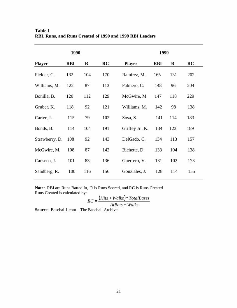
runners than who was the best at driving in runners (Grabiner ). Table 1 compares the

Runs Created (RC), RBI, and RUNS of the top ten RBI producers in 1990 and 1999. RBI

hitters usually bat third or fourth in the batting order and are hitting with people on base.

For example, in 1990 Ryne Sandberg had more Runs than RBI’s, and that is probably

because he hit second and was driven in by other good hitters. It is clear that RBI’s and

Runs scored are not the only determinants of Runs Created. As Bonds and Sandberg

indicate, on base percentage and speed can increase your runs created. Runs Created

shows more of the complete player in offensive characteristics.

For pitchers, individual performance is measured by Earned Run Average (ERA).

Earned run average is calculated by:

chedInningsPitEarnedRunsERA 9*=

ERA measures the average number of runs per nine innings pitched. For example, a

pitcher with an ERA of 3.65 means that the pitcher gives up 3.65 earned runs per nine

innings. An earned run is a run scored without any errors. In contrast, Scully (1974) and

others claim a pitchers strikeout-walk ratio is the best measure of performance. The

purpose of a pitcher, however, is to stop the other team from scoring. This could come in

12

the form of strikeouts, ground balls, or fly balls. According to Zimbalist (199) and

MacDonald (1994), ERA is highly significantly related to winning percentage and they

argue it is the preferred pitching statistic.

3. Descriptive Characteristics

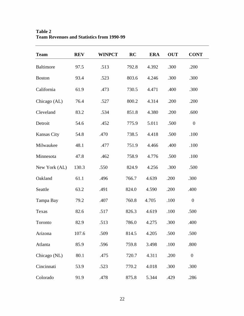
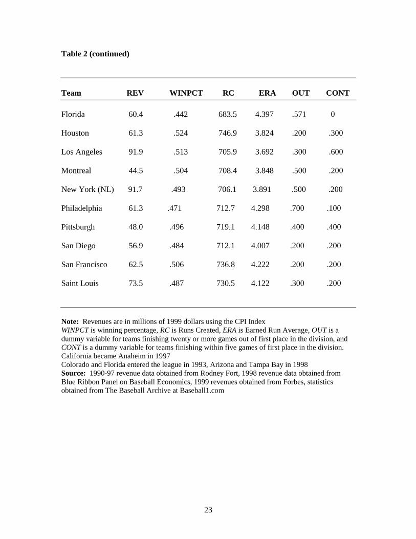
The descriptive statistics for team revenues over the 1990-99 period are given in

Table 2. The New York Yankees had the largest average revenue of 130 million dollars,

as well as the best winning percentage of .550. Colorado had the most runs created

(875.794) as well as the highest ERA at 5.344. Many give credit to the runs scored in

Colorado to the elevation and thin air. Demonstrating the saying that pitching wins

games, Atlanta had the lowest ERA at 3.498 and was also within 5 games of first 80% of

the time.

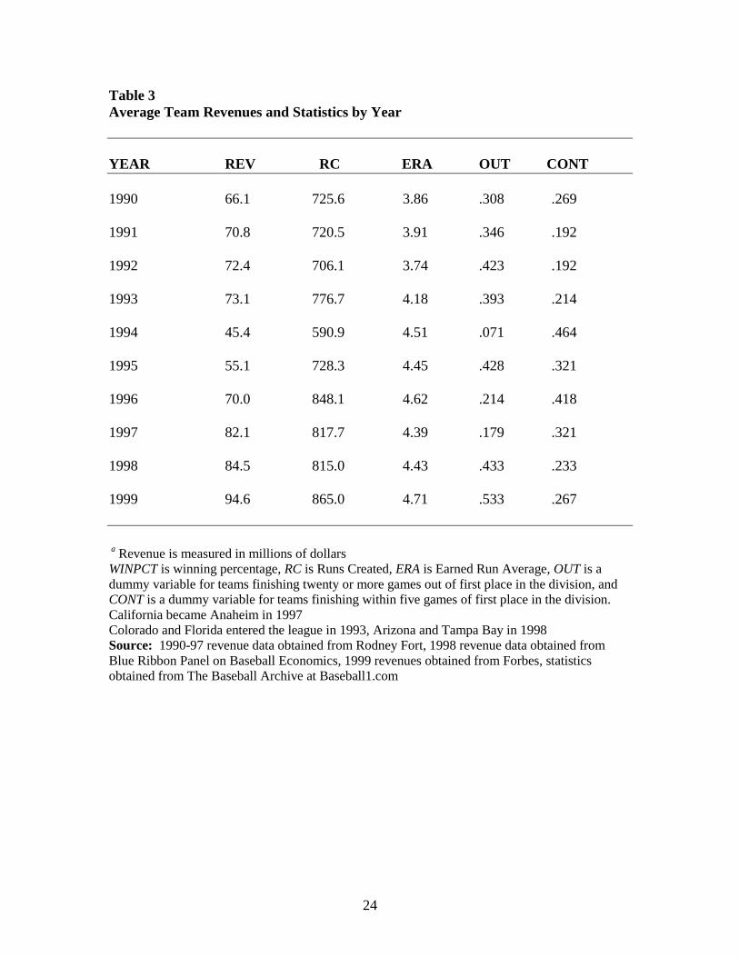
Table 3 shows the statistics for average team revenues and statistics over the ten-

year period. 1999 had the largest average revenue of $95 million and the strike shortened

year of 1994 had the lowest average revenue of $45 million. Runs created saw a great

increase in 1996 and has remained pretty steady since. ERA has seen a steady increase

over the years, partly due to the increased offensive production the game has achieved

over the years.

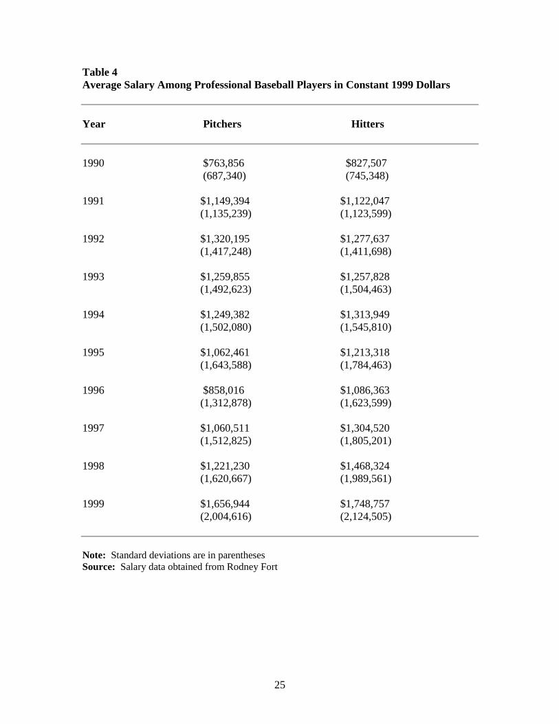
The average salary among professional baseball players is shown in Table 4.

Pitcher and hitter average real salaries remain pretty constant over the ten year span. As

the real salaries increase, the standard deviation also increases. This suggests that there

are some of the players that are making much more as the average real salaries increase.

As expected, the average real salaries were greatest in 1999 and lowest in 1990 and 1996.

13

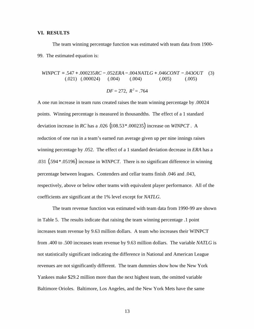
VI. RESULTS

The team winning percentage function was estimated with team data from 1900-

99. The estimated equation is:

OUTCONTNATLGERARCWINPCT 043.046.004.052.000235.547. −+−−+= (3)

(.021) (.000024) (.004) (.004) (.005) (.005)

DF = 272, 2R = .764 A one run increase in team runs created raises the team winning percentage by .00024

points. Winning percentage is measured in thousandths. The effect of a 1 standard

deviation increase in RC has a .026 ( )000235.*53.108 increase on WINPCT . A

reduction of one run in a team’s earned run average given up per nine innings raises

winning percentage by .052. The effect of a 1 standard deviation decrease in ERA has a

.031 ( )05196.*594. increase in WINPCT. There is no significant difference in winning

percentage between leagues. Contenders and cellar teams finish .046 and .043,

respectively, above or below other teams with equivalent player performance. All of the

coefficients are significant at the 1% level except for NATLG.

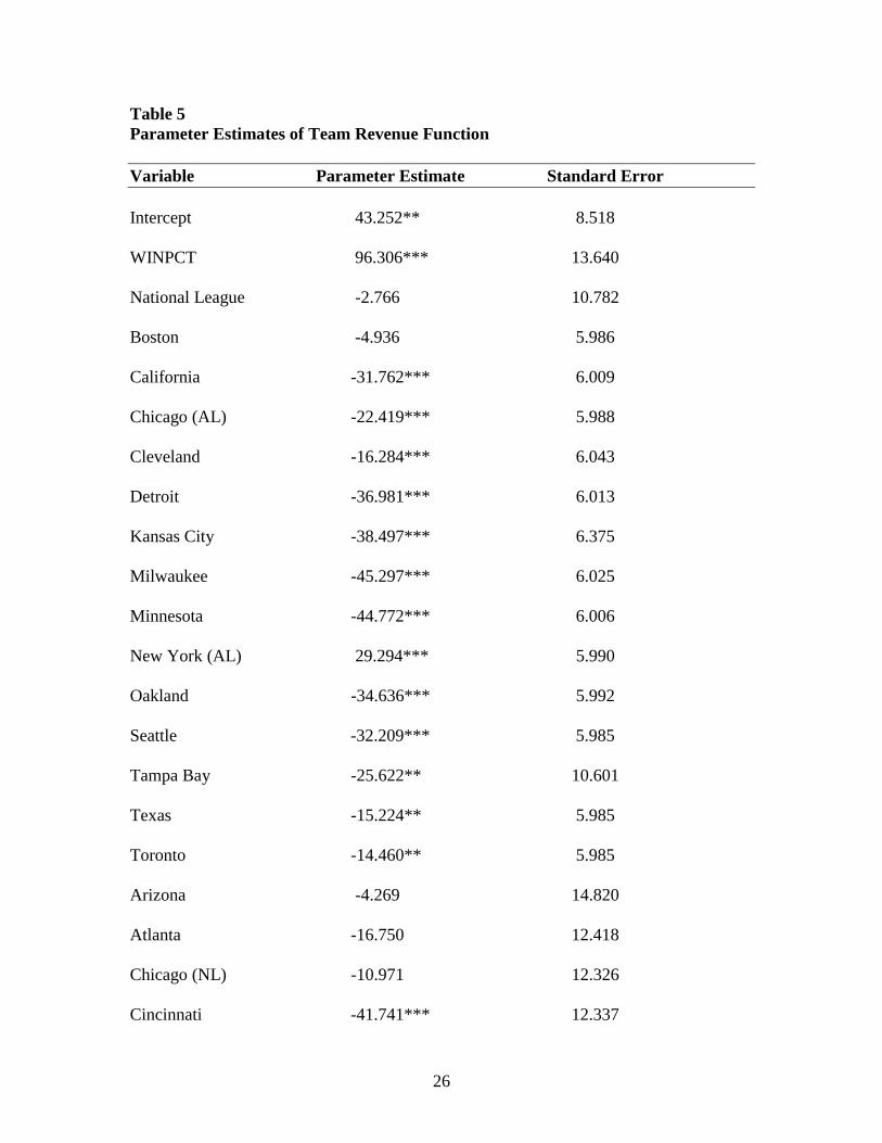
The team revenue function was estimated with team data from 1990-99 are shown

in Table 5. The results indicate that raising the team winning percentage .1 point

increases team revenue by 9.63 million dollars. A team who increases their WINPCT

from .400 to .500 increases team revenue by 9.63 million dollars. The variable NATLG is

not statistically significant indicating the difference in National and American League

revenues are not significantly different. The team dummies show how the New York

Yankees make $29.2 million more than the next highest team, the omitted variable

Baltimore Orioles. Baltimore, Los Angeles, and the New York Mets have the same

14

revenues with the other teams making anywhere from $10-$49 million dollars less than

Baltimore. The year dummies show that the year of the strike (1994-95) had an effect on

team revenues. Team revenues were considerably lower the years of the strike, but

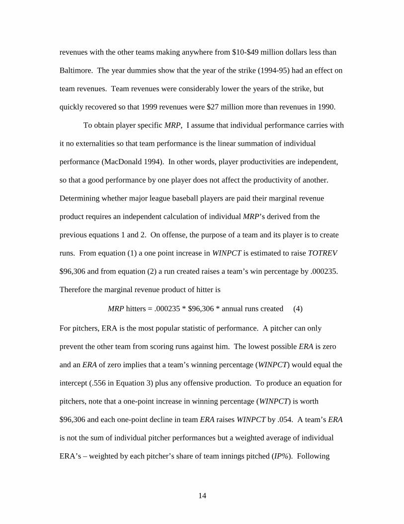
quickly recovered so that 1999 revenues were $27 million more than revenues in 1990.

To obtain player specific MRP, I assume that individual performance carries with

it no externalities so that team performance is the linear summation of individual

performance (MacDonald 1994). In other words, player productivities are independent,

so that a good performance by one player does not affect the productivity of another.

Determining whether major league baseball players are paid their marginal revenue

product requires an independent calculation of individual MRP’s derived from the

previous equations 1 and 2. On offense, the purpose of a team and its player is to create

runs. From equation (1) a one point increase in WINPCT is estimated to raise TOTREV

$96,306 and from equation (2) a run created raises a team’s win percentage by .000235.

Therefore the marginal revenue product of hitter is

MRP hitters = .000235 * $96,306 * annual runs created (4) For pitchers, ERA is the most popular statistic of performance. A pitcher can only

prevent the other team from scoring runs against him. The lowest possible ERA is zero

and an ERA of zero implies that a team’s winning percentage (WINPCT) would equal the

intercept (.556 in Equation 3) plus any offensive production. To produce an equation for

pitchers, note that a one-point increase in winning percentage (WINPCT) is worth

$96,306 and each one-point decline in team ERA raises WINPCT by .054. A team’s ERA

is not the sum of individual pitcher performances but a weighted average of individual

ERA’s – weighted by each pitcher’s share of team innings pitched (IP%). Following

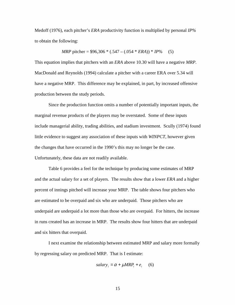
15

Medoff (1976), each pitcher’s ERA productivity function is multiplied by personal IP%

to obtain the following:

MRP pitcher = $96,306 * (.547 – (.054 * ERA)) * IP% (5)

This equation implies that pitchers with an ERA above 10.30 will have a negative MRP.

MacDonald and Reynolds (1994) calculate a pitcher with a career ERA over 5.34 will

have a negative MRP. This difference may be explained, in part, by increased offensive

production between the study periods.

Since the production function omits a number of potentially important inputs, the

marginal revenue products of the players may be overstated. Some of these inputs

include managerial ability, trading abilities, and stadium investment. Scully (1974) found

little evidence to suggest any association of these inputs with WINPCT, however given

the changes that have occurred in the 1990’s this may no longer be the case.

Unfortunately, these data are not readily available.

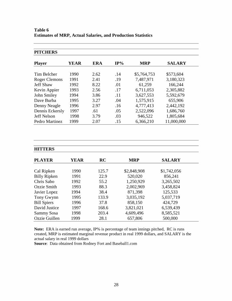
Table 6 provides a feel for the technique by producing some estimates of MRP

and the actual salary for a set of players. The results show that a lower ERA and a higher

percent of innings pitched will increase your MRP. The table shows four pitchers who

are estimated to be overpaid and six who are underpaid. Those pitchers who are

underpaid are underpaid a lot more than those who are overpaid. For hitters, the increase

in runs created has an increase in MRP. The results show four hitters that are underpaid

and six hitters that overpaid.

I next examine the relationship between estimated MRP and salary more formally

by regressing salary on predicted MRP. That is I estimate:

iii eMRPsalary ++= µα (6)

16

where salary i is the salary of player i and iMRP is the estimated MRP. If baseball

players are paid their marginal revenue products and the estimate of MRP is accurate, the

estimate of µ should be equal to one: a one-dollar increase in MRP should result in a

one-dollar increase in salary. To the extent there is measurement error in the estimate of

MRP, estimates of µ will be biased downward.

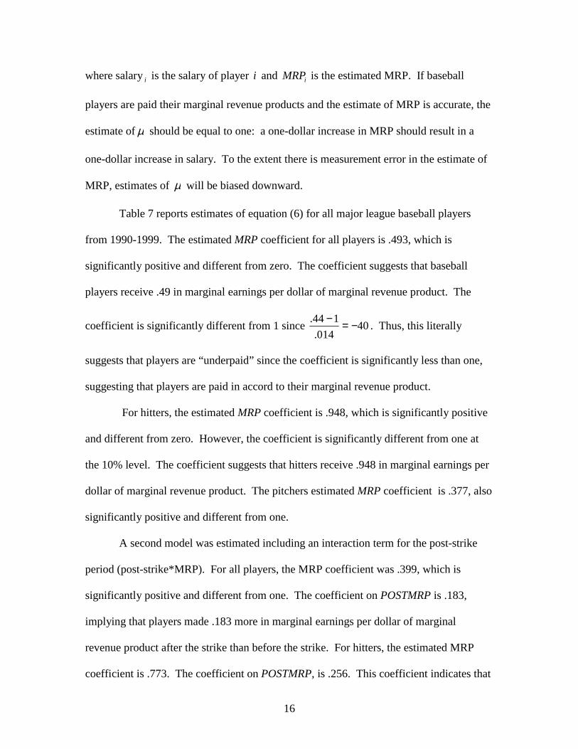
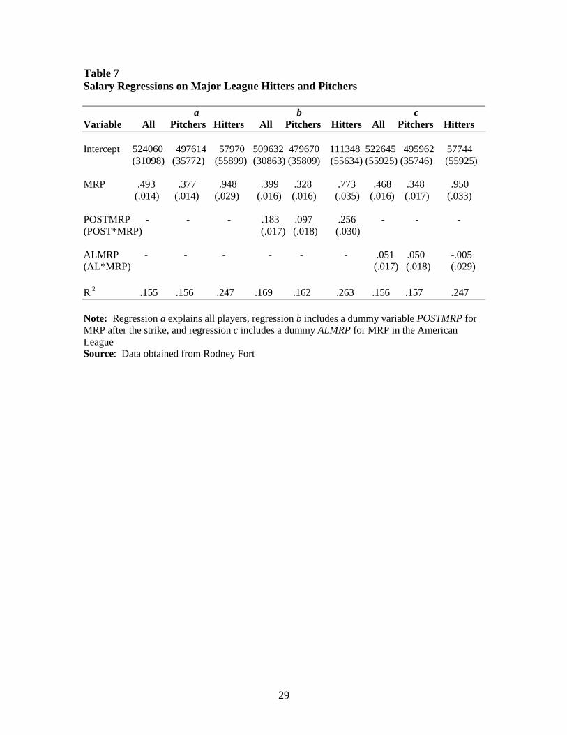
Table 7 reports estimates of equation (6) for all major league baseball players

from 1990-1999. The estimated MRP coefficient for all players is .493, which is

significantly positive and different from zero. The coefficient suggests that baseball

players receive .49 in marginal earnings per dollar of marginal revenue product. The

coefficient is significantly different from 1 since 40014.

144. −=− . Thus, this literally

suggests that players are “underpaid” since the coefficient is significantly less than one,

suggesting that players are paid in accord to their marginal revenue product.

For hitters, the estimated MRP coefficient is .948, which is significantly positive

and different from zero. However, the coefficient is significantly different from one at

the 10% level. The coefficient suggests that hitters receive .948 in marginal earnings per

dollar of marginal revenue product. The pitchers estimated MRP coefficient is .377, also

significantly positive and different from one.

A second model was estimated including an interaction term for the post-strike

period (post-strike*MRP). For all players, the MRP coefficient was .399, which is

significantly positive and different from one. The coefficient on POSTMRP is .183,

implying that players made .183 more in marginal earnings per dollar of marginal

revenue product after the strike than before the strike. For hitters, the estimated MRP

coefficient is .773. The coefficient on POSTMRP, is .256. This coefficient indicates that

17

hitters received .256 more in marginal earnings per dollar of marginal revenue product

after the strike than before the strike. For pitchers, the estimated MRP coefficient is

.328 and is significant. The estimated POSTMRP coefficient is .097. Pitchers received

.097 more in marginal earnings per dollar of marginal revenue product after the strike.

Therefore the strike played a big role in the increase of major league players’ salaries, or

at least increased the correlation between salary and MRP.

The next regression included an interaction term including American

League*MRP (ALMRP). All players had a MRP coefficient of .468. The coefficient on

ALMRP was .051, which is significantly different from zero. Therefore players in the

American League make .051 more per dollar of marginal revenue product. Pitchers have

a MRP coefficient of .348 and a ALMRP coefficient of .050, which is significantly

different from zero. Hitters have a MRP coefficient of .950, which is not significantly

different from one, and an ALMRP coefficient of -.005. The coefficients on ALMRP

show that pitching is more valued in the American League or that there is a higher

premium placed on a given ERA.

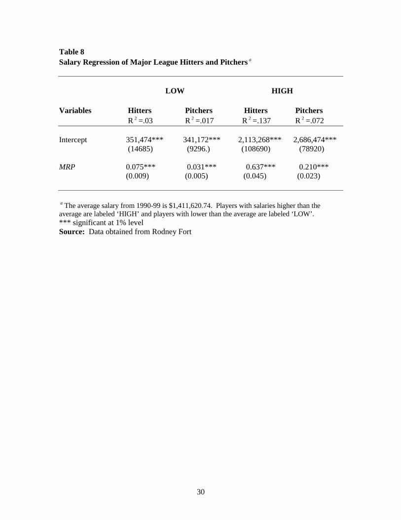
The final salary regressions are run with hitters and pitchers who have salaries

above and below the average salary of $1,400,000. The results are found in Table 8.

Beginning with the upper salary bracket, hitters have an estimated MRP coefficient of

.637, which is significant. Hitters making above the average salary receive .637 more in

marginal earnings per dollar of marginal revenue product. This coefficient suggests that

hitters above the average salary are underpaid. Hitters who make below the average

salary have an estimated MRP coefficient of .075. This suggests that hitters making

below the average salary are much underpaid. For pitchers, the estimated MRP

18

coefficient is .210 and significant for those making above the average salary. Pitchers

making below the average salary have an estimated MRP coefficient of .031. This

estimate is significant. Pitchers below the average salary only make .03 earnings per

dollar of marginal revenue product, indicating that they are greatly underpaid. These

results show that both tiers of major league baseball players are greatly underpaid, but,

consistent with previous research, younger players are paid a salary that is well below

their contribution to team revenues as compared to older players.

VII. Conclusion The purpose of this study is to determine if professional baseball players are paid

accordingly to their marginal product. Estimating a team revenue regression and a

winning percentage regression I calculate a player’s marginal revenue product. The

results indicate that professional baseball players are underpaid as compared to their

contributions to team revenues. Players were paid closer to their marginal product post-

strike and MRP’s were about the same between leagues.

The goal of a well-designed sports league is to produce sufficient competitive

balance. By this standard, Major League Baseball is not now well designed. What

makes its current economic structure weak in the long run is that, year after year, too

many clubs know in spring training that they have no realistic hope of reaching

postseason play. This structure is negatively affecting the ability of most clubs to

increase revenues and achieve operating stability. Too many clubs in low-revenue

markets can only expect to compete for postseason berths if ownership is willing to incur

staggering operating losses to subsidize a competitive player payroll (Levin et al. 2000).

19

If my MRP estimates are reasonable, there must be some explanations as to why

owners are underpaying players as compared to his marginal revenue product. If my

MRP estimates are correct, then exploitation of the players exists. The owners can

misgauge a player’s worth. This could lead to the underestimating of player expectations

by the owners. These could easily lead to the underpayment of professional baseball

players. If my MRP estimates are wrong, it could be the result of econometric bias.

Another problem could be the use of wrong variables. Runs Created and ERA may not

be the best statistic to measure offensive and pitching performance.

The Blue Ribbon Panel on Baseball Economics describes how the league needs to

keep salaries low. They make suggestions to help out owners relative to the players. My

results suggest the opposite. My results indicate that the league needs to raise the

salaries. If my estimates are correct, the focus should be on helping players, relative to

the owners, to help them receive their marginal revenue product.

20

References

Grabiner, David, “The Sabermetric Manifesto,” The Baseball Archive, www.baseball.com. Krautman, Anthony C., “What’s Wrong with Scully-Estimates of a Player’s Marginal

Revenue Product,” Economic Inquiry, Vol. 37, No.2, April 1999, 369-381 Levin, Richard C., George J. Mitchell, Paul A. Volcker, and George F. Will, The Report

of the Independent Members of the Commissioner’s Blue Ribbon Panel on Baseball Economics, July 2000

MacDonald, Don N. and Morgan O. Reynolds, “Are Baseball Players Paid their

Marginal Products?” Managerial and Decision Economics, Vol. 15, 1994, 443-457

Scully, Gerald W. “Pay and Performance in Major League Baseball,” The American

Economic Review, Vol. 64, No. 6, December 1974, 915-930 Staudohar, Paul D. “Salary Caps in Professional Team Sports,” Compensation and

Working Conditions, Spring 1998, 3-9 Zimbalist, Andrew. “Salaries and Performance: Beyond the Scully Model,” Diamonds

are Forever, The Business of Baseball. Sommers, Washington, D.C., 1992, 109-133

21

Table 1 RBI, Runs, and Runs Created of 1990 and 1999 RBI Leaders

1990 1999 Player RBI R RC Player RBI R RC Fielder, C. 132 104 170 Ramirez, M. 165 131 202 Williams, M. 122 87 113 Palmero, C. 148 96 204 Bonilla, B. 120 112 129 McGwire, M 147 118 229 Gruber, K. 118 92 121 Williams, M. 142 98 138 Carter, J. 115 79 102 Sosa, S. 141 114 183 Bonds, B. 114 104 191 Griffey Jr., K. 134 123 189 Strawberry, D. 108 92 143 DelGado, C. 134 113 157 McGwire, M. 108 87 142 Bichette, D. 133 104 138 Canseco, J. 101 83 136 Guerrero, V. 131 102 173 Sandberg, R. 100 116 156 Gonzlales, J. 128 114 155 Note: RBI are Runs Batted In, R is Runs Scored, and RC is Runs Created Runs Created is calculated by:

( )WalksAtBatsTotalBasesWalksHitsRC

++= *

Source: Baseball1.com – The Baseball Archive

22

Table 2 Team Revenues and Statistics from 1990-99 Team REV WINPCT RC ERA OUT CONT Baltimore 97.5 .513 792.8 4.392 .300 .200 Boston 93.4 .523 803.6 4.246 .300 .300 California 61.9 .473 730.5 4.471 .400 .300 Chicago (AL) 76.4 .527 800.2 4.314 .200 .200 Cleveland 83.2 .534 851.8 4.380 .200 .600 Detroit 54.6 .452 775.9 5.011 .500 0 Kansas City 54.8 .470 738.5 4.418 .500 .100 Milwaukee 48.1 .477 751.9 4.466 .400 .100 Minnesota 47.8 .462 758.9 4.776 .500 .100 New York (AL) 130.3 .550 824.9 4.256 .300 .500 Oakland 61.1 .496 766.7 4.639 .200 .300 Seattle 63.2 .491 824.0 4.590 .200 .400 Tampa Bay 79.2 .407 760.8 4.705 .100 0 Texas 82.6 .517 826.3 4.619 .100 .500 Toronto 82.9 .513 786.0 4.275 .300 .400 Arizona 107.6 .509 814.5 4.205 .500 .500 Atlanta 85.9 .596 759.8 3.498 .100 .800 Chicago (NL) 80.1 .475 720.7 4.311 .200 0 Cincinnati 53.9 .523 770.2 4.018 .300 .300 Colorado 91.9 .478 875.8 5.344 .429 .286

23

Table 2 (continued) Team REV WINPCT RC ERA OUT CONT Florida 60.4 .442 683.5 4.397 .571 0 Houston 61.3 .524 746.9 3.824 .200 .300 Los Angeles 91.9 .513 705.9 3.692 .300 .600 Montreal 44.5 .504 708.4 3.848 .500 .200 New York (NL) 91.7 .493 706.1 3.891 .500 .200 Philadelphia 61.3 .471 712.7 4.298 .700 .100 Pittsburgh 48.0 .496 719.1 4.148 .400 .400 San Diego 56.9 .484 712.1 4.007 .200 .200 San Francisco 62.5 .506 736.8 4.222 .200 .200 Saint Louis 73.5 .487 730.5 4.122 .300 .200 Note: Revenues are in millions of 1999 dollars using the CPI Index WINPCT is winning percentage, RC is Runs Created, ERA is Earned Run Average, OUT is a dummy variable for teams finishing twenty or more games out of first place in the division, and CONT is a dummy variable for teams finishing within five games of first place in the division. California became Anaheim in 1997 Colorado and Florida entered the league in 1993, Arizona and Tampa Bay in 1998 Source: 1990-97 revenue data obtained from Rodney Fort, 1998 revenue data obtained from Blue Ribbon Panel on Baseball Economics, 1999 revenues obtained from Forbes, statistics obtained from The Baseball Archive at Baseball1.com

24

Table 3 Average Team Revenues and Statistics by Year YEAR REV RC ERA OUT CONT 1990 66.1 725.6 3.86 .308 .269 1991 70.8 720.5 3.91 .346 .192 1992 72.4 706.1 3.74 .423 .192 1993 73.1 776.7 4.18 .393 .214 1994 45.4 590.9 4.51 .071 .464 1995 55.1 728.3 4.45 .428 .321 1996 70.0 848.1 4.62 .214 .418 1997 82.1 817.7 4.39 .179 .321 1998 84.5 815.0 4.43 .433 .233 1999 94.6 865.0 4.71 .533 .267 a Revenue is measured in millions of dollars WINPCT is winning percentage, RC is Runs Created, ERA is Earned Run Average, OUT is a dummy variable for teams finishing twenty or more games out of first place in the division, and CONT is a dummy variable for teams finishing within five games of first place in the division. California became Anaheim in 1997 Colorado and Florida entered the league in 1993, Arizona and Tampa Bay in 1998 Source: 1990-97 revenue data obtained from Rodney Fort, 1998 revenue data obtained from Blue Ribbon Panel on Baseball Economics, 1999 revenues obtained from Forbes, statistics obtained from The Baseball Archive at Baseball1.com

25

Table 4 Average Salary Among Professional Baseball Players in Constant 1999 Dollars Year Pitchers Hitters 1990 $763,856 $827,507 (687,340) (745,348) 1991 $1,149,394 $1,122,047 (1,135,239) (1,123,599) 1992 $1,320,195 $1,277,637 (1,417,248) (1,411,698) 1993 $1,259,855 $1,257,828 (1,492,623) (1,504,463) 1994 $1,249,382 $1,313,949 (1,502,080) (1,545,810) 1995 $1,062,461 $1,213,318 (1,643,588) (1,784,463) 1996 $858,016 $1,086,363 (1,312,878) (1,623,599) 1997 $1,060,511 $1,304,520 (1,512,825) (1,805,201) 1998 $1,221,230 $1,468,324 (1,620,667) (1,989,561) 1999 $1,656,944 $1,748,757 (2,004,616) (2,124,505) Note: Standard deviations are in parentheses Source: Salary data obtained from Rodney Fort

26

Table 5 Parameter Estimates of Team Revenue Function Variable Parameter Estimate Standard Error Intercept 43.252** 8.518

WINPCT 96.306*** 13.640

National League -2.766 10.782

Boston -4.936 5.986

California -31.762*** 6.009

Chicago (AL) -22.419*** 5.988

Cleveland -16.284*** 6.043

Detroit -36.981*** 6.013

Kansas City -38.497*** 6.375

Milwaukee -45.297*** 6.025

Minnesota -44.772*** 6.006

New York (AL) 29.294*** 5.990

Oakland -34.636*** 5.992

Seattle -32.209*** 5.985

Tampa Bay -25.622** 10.601

Texas -15.224** 5.985

Toronto -14.460** 5.985

Arizona -4.269 14.820

Atlanta -16.750 12.418

Chicago (NL) -10.971 12.326

Cincinnati -41.741*** 12.337

27

Table 5 (continued) Variable Parameter Estimate Standard Error Colorado .109 12.615

Florida -27.950** 12.629

Houston -34.481*** 12.338

Los Angeles -2.816 12.332

Montreal -49.302*** 12.328

New York (NL) -1.098 12.326

Philadelphia -29.318** 12.327

Pittsburgh -45.050*** 12.327

San Diego -34.972*** 12.326

San Francisco -31.527** 12.329

Saint Louis -18.689 12.326

1991 4.672 3.712

1992 6.273* 3.712

1993 6.358* 3.655

1994 -21.286*** 3.655

1995 -11.636*** 3.655

1996 3.340 3.655

1997 15.439*** 3.655

1998 17.284*** 3.648

1999 27.436*** 3.648

Note: *, **, *** indicate significance at the 90%, 95%, and 99* levels, respectively Dependent variable is annual team revenue in millions of 1990 dollars Source: 90-97 revenues-Rodney Fort, 1998 revenues-Blue Ribbon Panel, 1999 revenues-Forbes

28

Table 6 Estimates of MRP, Actual Salaries, and Production Statistics

PITCHERS Player YEAR ERA IP% MRP SALARY Tim Belcher 1990 2.62 .14 $5,764,753 $573,604 Roger Clemons 1991 2.41 .19 7,487,971 3,180,323 Jeff Shaw 1992 8.22 .01 61,259 166,244 Kevin Appier 1993 2.56 .17 6,711,053 2,305,882 John Smiley 1994 3.86 .11 3,627,553 5,592,679 Dave Burba 1995 3.27 .04 1,575,915 655,906 Denny Neagle 1996 2.97 .16 4,777,413 2,442,192 Dennis Eckersly 1997 .61 .05 2,522,096 1,686,760 Jeff Nelson 1998 3.79 .03 946,522 1,805,684 Pedro Martinez 1999 2.07 .15 6,366,210 11,000,000

HITTERS PLAYER YEAR RC MRP SALARY Cal Ripken 1990 125.7 $2,848,908 $1,742,056 Billy Ripken 1991 22.9 520,020 856,241 Chris Sabo 1992 55.2 1,250,929 3,265,502 Ozzie Smith 1993 88.3 2,002,969 3,458,824 Javier Lopez 1994 38.4 871,398 125,533 Tony Gwynn 1995 133.9 3,035,192 5,037,719 Bill Spiers 1996 37.8 858,150 424,729 David Justice 1997 168.6 3,821,021 6,539,439 Sammy Sosa 1998 203.4 4,609,496 8,585,521 Ozzie Guillen 1999 28.1 657,806 500,000 Note: ERA is earned run average, IP% is percentage of team innings pitched, RC is runs created, MRP is estimated marginal revenue product in real 1999 dollars, and SALARY is the actual salary in real 1999 dollars Source: Data obtained from Rodney Fort and Baseball1.com

29

Table 7 Salary Regressions on Major League Hitters and Pitchers a b c Variable All Pitchers Hitters All Pitchers Hitters All Pitchers Hitters Intercept 524060 497614 57970 509632 479670 111348 522645 495962 57744 (31098) (35772) (55899) (30863) (35809) (55634) (55925) (35746) (55925) MRP .493 .377 .948 .399 .328 .773 .468 .348 .950 (.014) (.014) (.029) (.016) (.016) (.035) (.016) (.017) (.033) POSTMRP - - - .183 .097 .256 - - - (POST*MRP) (.017) (.018) (.030) ALMRP - - - - - - .051 .050 -.005 (AL*MRP) (.017) (.018) (.029) R 2 .155 .156 .247 .169 .162 .263 .156 .157 .247 Note: Regression a explains all players, regression b includes a dummy variable POSTMRP for MRP after the strike, and regression c includes a dummy ALMRP for MRP in the American League Source: Data obtained from Rodney Fort

30

Table 8 Salary Regression of Major League Hitters and Pitchers a LOW HIGH Variables Hitters Pitchers Hitters Pitchers R 2 =.03 R 2 =.017 R 2 =.137 R 2 =.072 Intercept 351,474*** 341,172*** 2,113,268*** 2,686,474*** (14685) (9296.) (108690) (78920) MRP 0.075*** 0.031*** 0.637*** 0.210*** (0.009) (0.005) (0.045) (0.023) a The average salary from 1990-99 is $1,411,620.74. Players with salaries higher than the average are labeled ‘HIGH’ and players with lower than the average are labeled ‘LOW’. *** significant at 1% level Source: Data obtained from Rodney Fort