Temperature differences between the hemispheres and ice age

ClickHere

for

FullArticle

Temperature differences between the hemispheres and ice ageclimate variability

J. R. Toggweiler1 and David W. Lea2

Received 4 March 2009; revised 1 December 2009; accepted 7 January 2010; published 15 June 2010.

[1] The Earth became warmer and cooler during the ice ages along with changes in the Earth’s orbit, but theorbital changes themselves are not nearly large enough to explain the magnitude of the warming andcooling. Atmospheric CO2 also rose and fell, but again, the CO2 changes are rather small in relation to thewarming and cooling. So, how did the Earth manage to warm and cool by so much? Here we argue that, forthe big transitions at least, the Earth did not warm and cool as a single entity. Rather, the south warmedinstead at the expense of a cooler north through massive redistributions of heat that were set off by theorbital forcing. Oceanic CO2 was vented up to the atmosphere by the same redistributions. The north thenwarmed later in response to higher CO2 and a reduced albedo from smaller ice sheets. This form of north‐south displacement is actually very familiar, as it is readily observed during the Younger Dryas interval13,000 years ago and in the various millennial‐scale events over the last 90,000 years.

Citation: Toggweiler, J. R., and D. W. Lea (2010), Temperature differences between the hemispheres and ice age climatevariability, Paleoceanography, 25, PA2212, doi:10.1029/2009PA001758.

1. Introduction

[2] Ice cores from Antarctica have produced two kinds ofrecords. Records from the center of Antarctic extend back650,000 years and cover six long cycles [Petit et al., 1999;Siegenthaler et al., 2005]. Records from the coast areshorter in time but resolve more of the variability over thelast 90,000 years [Indermühle et al., 2000; Monnin et al.,2001; EPICA Community Members, 2006; Ahn and Brook,2008]. Both kinds of records show that Antarctica warmedand cooled along with the level of CO2 in the atmosphere.The problem is that the relationship between Antarctictemperatures and atmospheric CO2 has been interpreted verydifferently over the two time scales.[3] Figure 1 [from Ahn and Brook, 2008] exemplifies

the shorter records. Temperature and CO2 records fromAntarctica (Figures 1b and 1c) are shown along with recordsfrom Greenland in the Northern Hemisphere. The Antarcticrecords feature a series of “millennial‐scale events,” iden-tified by the labels A1–A7, in which the temperatures inAntarctica and the level of CO2 in the atmosphere rise andfall together over some 5000–10,000 years.[4] During the millennial events, Greenland cools while

Antarctica warms, and vice versa. The CO2 increases alsolag slightly behind the warmings in Antarctica, as shown inmore detail by Ahn and Brook [2007]. Thus, the greenhouseeffect from atmospheric CO2 clearly did not make Green-

land or Antarctica warmer and cooler over the millennialtime scale, and a mechanism is needed to explain why thetemperatures in Antarctica rose and fell along with atmo-spheric CO2.[5] The long records from the center of Antarctica are

better known [Petit et al., 1999; Siegenthaler et al., 2005];two such records are reproduced in section 5. They featurebig transitions every 100,000 years or so in which Antarc-tica warms by up to 10°C while the level of CO2 in theatmosphere rises by up to 100 ppm. Figure 1 includes themost recent big transition, which took place between 10,000and 20,000 years ago.[6] One expects the warming and cooling from atmo-

spheric CO2 to be a global phenomenon, and indeed thewhole Earth seems to warm and cool together over the longertime scales. Hence, it is natural to assume that the CO2‐temperature relationship in the long records from Antarcticais causal, i.e., that the increases in atmospheric CO2 warmedAntarctica and the rest of the planet [Genthon et al., 1987;Lorius et al., 1990; Hansen et al., 2007]. But the samerelationship is seen during the millennial events, and theCO2‐temperature relationship during the millennial events isclearly not causal. Can two such disparate views both becorrect?[7] A close look shows that Antarctica and the polar north

did not warm and cool at the same times; the two hemi-spheres became warm together over the longer cycles butonly after the big transitions in Antarctica had alreadyoccurred. Both kinds of transitions, millennial and longterm, seem to involve displacements of heat that allow thesouth to warm at the expense of the north. The displace-ments over the longer cycles are simply larger versions ofthe millennial displacements. Atmospheric CO2 rises andfalls via the displacements that warm and cool the south.

1Geophysical Fluid Dynamics Laboratory, NOAA, Princeton, NewJersey, USA.

2Department of Earth Science and Marine Science Institute,University of California, Santa Barbara, California, USA.

Copyright 2010 by the American Geophysical Union.0883‐8305/10/2009PA001758

PALEOCEANOGRAPHY, VOL. 25, PA2212, doi:10.1029/2009PA001758, 2010

PA2212 1 of 14

http://dx.doi.org/10.1029/2009PA001758

[8] For the purposes of this paper, the phrase “big tran-sitions” is an explicit reference to the abrupt warmings andCO2 increases seen in the Antarctic ice cores. “Termina-tions” refer to the demise of the northern ice sheets. The ageof a termination is the time when the northern ice sheets arewasting away most rapidly.

2. North‐South Temperature DifferencesDuring the Millennial Events

[9] The millennial‐scale events in Antarctica (Figure 1)were initiated by inputs of fresh water that weakened themeridional overturning circulation in the Atlantic (hereafterAMOC) [Bond et al., 1993; Blunier et al., 1998]. Theweakened overturning cooled the North Atlantic and initi-ated an out‐of‐phase warming in the Southern Hemisphere.Broecker [1998] called this out‐of‐phase relationship the“bipolar seesaw.”[10] According to Broecker [1998], the ocean’s over-

turning is maintained by the downward mixing of heatacross the thermocline, which allows old lighter water to bedisplaced upward by younger denser waters flowing into theinterior from the poles. If the production of denser water isreduced in one hemisphere it must increase in the other tocompensate. From this perspective, the seesaw should makeone hemisphere warmer and then the other. This is not quitewhat we see, however.[11] The Northern Hemisphere is systematically warmer

than the Southern Hemisphere, especially in the sectorcontaining the Atlantic Ocean (Figure 2). So, when thesouth warms during the millennial events, the temperature

Figure 1. Millennial‐scale events recorded in ice core records from Greenland and Antarctica over the last90,000 years. (a) Proxy for air temperature over Greenland. (b) Proxy for air temperature over Antarctica.(c) Atmospheric CO2 recorded in Antarctica. (d) Atmospheric methane fromGreenland (green) and Antarc-tica (brown). Vertical bars denote Heinrich stadials H3–H6. Blue labels A1–A7 denote millennial‐scaleevents in which the level of CO2 in the atmosphere increases while Antarctica warms [Blunier andBrook, 2001]. Greenland warms abruptly as Antarctica cools after warm peaks A1–A7. From Ahn andBrook [2008, Figure 1]. Reprinted with permission from AAAS.

Figure 2. Zonally averaged sea surface temperature (SST)plotted as a departure from the mean SST for each latitude.The bold blue curve is derived from observed SSTs in theAtlantic Ocean. The green curve is derived from observedSSTs over the whole ocean. The red curve represents theSST difference between two model simulations, one with acircumpolar channel and an interhemispheric overturning cir-culation and one without. From Toggweiler and Bjornsson[2000, Figure 11]. Observed SSTs are averages of theupper 50 m in the Levitus [1982] climatology.

TOGGWEILER AND LEA: ICE AGE CLIMATE VARIABILITY PA2212PA2212

2 of 14

difference between the hemispheres is actually flattened oreven reversed. When Greenland is warm and Antarctica iscold after the millennial events, the north‐south temperaturedifference is enhanced.[12] This asymmetry is due to the Antarctic Circumpolar

Current (ACC) and the westerly winds that drive the ACCaround Antarctica. The ACC circles the globe in an east‐west channel that lies along the southern edge of the west-erly wind belt in the Southern Hemisphere. The stress fromthe westerlies on the ocean draws old deep water up to thesurface from the interior. New deep water sinks in the NorthAtlantic to compensate for the water drawn up by the windsin the south [Toggweiler and Samuels, 1995].[13] The ACC’s channel limits the poleward flow toward

Antarctica to depths below 2000 m. Thus, the winds overthe channel draw water from the middle depths of the oceanup to the surface and push it away to the north. As theupwelled water moves northward it takes up solar heat thatwould otherwise warm Antarctica and carries this heatacross the equator into the North Atlantic [Crowley, 1992;Toggweiler and Bjornsson, 2000]. This leads to a coolersouth and a warmer north.[14] So what made Antarctica warmer and cooler over

time? According to Toggweiler et al. [2006], the southernwesterlies at the Last Glacial Maximum (LGM) werelocated well to the north of the ACC. In this position, thewesterlies were not in a good position to draw middepthwater to the surface around Antarctica. As a result, the oceanaround Antarctica was very cold and was capped by a low‐salinity surface layer and a thick layer of sea ice. Accordingto Anderson et al. [2009], this began to change when aninput of icebergs and meltwater to the North Atlantic sup-pressed the AMOC and cooled the Northern Hemisphere ina way that caused the Intertropical Convergence Zone(ITCZ) and the trade winds in the tropics to shift to thesouth. The southern westerlies then shifted to the southalong with the trades. This shift put the southern westerliessquarely over the ACC, where they began drawing warmerand saltier middepth water to the surface. These warmishmiddepth waters displaced the near‐freezing surface watersaround Antarctica, melted back the sea ice, and warmed thecontinent.[15] The warmish middepth water was also high in CO2

that had been respired from sinking particles. So, southernwesterlies that were more squarely over the ACC drew moreCO2‐rich water to the surface, which then vented from theocean up to the atmosphere. This is how the temperatures inAntarctica and the level of CO2 in the atmosphere managedto rise together during the big transitions.

3. ITCZ, AMOC, and Precessional Cycle

[16] The precession of the Earth’s axis tends to make thesummers in one hemisphere warmer and cooler every23,000 years; summers in the opposite hemisphere arecooler and warmer in an antiphase way. Thus, precessionalcycles, like the millennial events, alter the temperaturecontrast between the hemispheres. The main new ideataken up in this paper is that precessional cycles andmillennial events are related and that they come together

every 100,000 years or so to produce to produce a giantmillennial event, which features an outsized warming ofAntarctica. Section 6 describes why these events are sounusual, but first an important distinction needs to be maderegarding the ways that themillennial events and precessionalcycles alter the north‐south contrast.[17] The ITCZ is a band of convection and enhanced

precipitation that is positioned above the warmest oceanwaters in the tropics. Because the Northern Hemisphere issystematically warmer than the Southern Hemisphere, theITCZ is generally found north of the equator. This leads to awell known asymmetry in the trade winds that flank theITCZ. During a typical year the northern trades are well tothe north of the equator between 10°N and 20°N, while thesouthern trades extend up to the equator from the south.During El Nino years, the ITCZ shifts toward the equatorfrom the north and the asymmetry is reduced. This causesthe southern trades to shift off the equator to the south andleads to especially warm temperatures along the equator inthe eastern equatorial Pacific.[18] The warming at the end of the last ice age took the

form of two steps [Monnin et al., 2001] in which Antarcticawarmed, cooled slightly for a couple thousand years, andthen warmed again. The two steps occurred during Heinrichstadial 1 (HS1) and the Younger Dryas (YD), times whenthe overturning circulation in the Atlantic (the AMOC) wassuppressed and the winters around the North Atlantic wereextremely cold [Denton et al., 2005]. Our claim, followingAnderson et al. [2009], is that a colder North Atlantic causedthe ITCZ and the trade winds to shift from their usualnorthern positions toward the equator and the south. Thesouthward displacement in the tropics then led to a morepoleward position for the westerly band further south.[19] The warm summers produced by the precessional

cycles have a similar effect that can be seen quite clearly inthe monsoons. In this case, the increased summer insolationwarms the land more than the adjacent ocean and causes theITCZ over the land to shift into the hemisphere that isreceiving more insolation [Wang et al., 2006]. Timmermannet al. [2007] show that the same sort of response extendsover the ocean. When the insolation is more intense duringnorthern summers, the SSTs north of the equator are warmerthan normal and the ITCZ and trade winds are shifted morestrongly into the Northern Hemisphere. When the insolationis more intense during southern summers, the temperaturecontrast across the equator is relatively flat and the ITCZand trade winds are shifted toward the equator and the south(Figure 3).[20] Lisiecki et al. [2008] show that the AMOC seems to

be stronger when the insolation during southern summers ismore intense, i.e., the AMOC is stronger when the north iscooler, which is opposite to the situation during the mil-lennial events. A widely used indicator of the strength of theAMOC over time is the changing d13C of the shells ofbenthic foraminifera from middepth Atlantic cores. A morepositive d13C is interpreted to reflect a greater input ofnorthern water that fills the middle depths of the Atlanticand pushes out the lighter bottom waters from Antarctica.Lisiecki et al. show that the d13C in middepth Atlantic cores


3 of 14

is more positive when the insolation during southernsummers is more intense.[21] The phasing identified by Lisiecki et al. [2008] is

supported by oceanic temperature changes in the middlelatitudes of the Southern Hemisphere. Barrows et al. [2007]have compiled SST proxies from four subantarctic cores andfind that SSTs are cooler between 130,000 and 70,000 yearsago when the insolation would otherwise have favoredwarmer summers. Antarctica is cooler at the same times[Kawamura et al., 2007]. The simplest explanation for thecooling at 45°S is that a stronger AMOC is carrying moreSouthern Hemisphere heat into the Northern Hemisphere atthese particular times. A stronger AMOC at these times isconsistent with Lisiecki et al.’s d13C results.[22] The reason why the AMOC responds to the preces-

sional forcing in this way is not entirely clear. The explana-tion to be entertained here is that the southern westerlies arestronger or more poleward shifted when the ITCZ is closer tothe equator, as they appear to be during the millennial events.But the AMOC, rather than being suppressed, is spun upinstead. This makes for an important distinction regarding theproperties measured in the Antarctic ice cores.[23] Figure 4 is a schematic illustration of the ocean’s

overturning circulation. During the millennial events, the redcirculation in Figure 4 (the AMOC) cannot spin up becauseit is being actively suppressed. Thus, in this case, polewardshifted westerlies spin up the deeper blue circulation insteadand draw middepth water from the blue domain up to thesurface right around Antarctica. The level of CO2 in theatmosphere increases along with the temperatures in Ant-arctica because a stronger blue circulation reduces the

accumulation of CO2 in the ocean’s interior from sinkingparticles [Ito and Follows, 2005; Toggweiler et al., 2006].[24] When the westerlies shift poleward in response to the

precessional forcing, and the AMOC is not suppressed, thered circulation appears to spin up instead. Antarctica doesnot warm in this case because southern heat is beingtransported to the Northern Hemisphere. Atmospheric CO2

does not increase either because the red circulation isenhanced in relation to the blue.

4. Evidence for Changes in Winds

[25] Haug et al. [2001] found that the inputs of titaniumand iron to sediments of the Cariaco Basin (11°N) on thecontinental shelf north of Venezuela were sharply reducedduring the Younger Dryas. They interpreted these reducedinputs as evidence for lower rainfall over northernmostSouth America (6°N–10°N) that was caused by a shift of theITCZ out of the 6°–10° band toward the south. Less rainfallover South America led to less river runoff and less titaniumand iron in Cariaco Basin sediments. Lea et al. [2003] showthat the surface waters over the Cariaco Basin were 3°C–4°Ccooler during HS1 and the YD and call for a rapid southwardshift of the ITCZ and the northern trades to explain thecooling. Similar ITCZ shifts seem to have occurred during allthe other millennial events [Peterson et al., 2000].[26] Haug et al. [2001] also found that the ITCZ and the

trade winds were shifted northward during the early Holocenewhen the northern summer insolation was at a maximum. The

Figure 4. Diagram illustrating the ocean’s overturning cir-culation and its relationship to atmospheric CO2. The over-turning is reduced to two components, a northern sourcedcirculation (red) and a deeper southern sourced circulation(blue). Both circulations are closed via upwelling withinthe box labeled DP/ACC (Drake Passage/Antarctic Circum-polar Current). Nutrient supply via the red circulation givesrise to CO2 uptake from the atmosphere and sinking parti-cles (brown squiggly lines), from which CO2 is respired inthe interior. CO2 accumulates in the blue domain when aweak blue circulation impedes the venting of respired CO2

back up to the atmosphere. The level of CO2 in the atmo-sphere rises when the blue circulation is strong in relationto the red. From Toggweiler et al. [2006].

Figure 3. Sea surface temperature difference between 5°N–12°N and 5°S–12°S in the eastern equatorial Pacific over thelast 140,000 years in response to orbitally induced insolationchanges. Result of a model simulation. The north is warm-est in relation to the south when the closest approach of theEarth to the Sun (perihelion) occurs during northern sum-mer. The SST difference is close to zero when the perihe-lion occurs in southern summer. From Timmermann et al.[2007, Figure 4].


4 of 14

ITCZ and the trades have since shifted back toward theequator as the insolation is stronger now during southernsummers than during northern summers. This supports theidea that the ITCZ responds in similar ways to changes in thetemperature contrast across the equator, whether by the pre-cessional forcing or the millennial events.[27] In a study of the sediment composition at ODP site

1233, Lamy et al. [2007] found that the surface waters offthe coast of Chile warmed rather abruptly during HS1 andthe YD in a way that is similar to the two warming steps inAntarctica. ODP site 1233 is located at 41°S in the transitionzone between warm subtropical waters and the cooler watersalong the northern edge of the ACC. Lamy et al. argued thata poleward shift of the westerlies at these times displaced thecooler ACC waters to the south and brought about thewarming off Chile. As with the ITCZ records above, similarwarmings occurred off the coast of Chile during all the othermillennial events [Kaiser et al., 2005].[28] Anderson et al. [2009] show that the poleward shift

of the westerlies extended into the zone around Antarctica.Anderson et al. discovered two pulses of opal deposition inthe region south of the Antarctic Polar Front (53°S–62°S)that took place during HS1 and the YD. The rate of opalburial during the two pulses was about five times larger thanthe rate of burial during the LGM (just prior to the twopulses). This points to a massive change in upwelling thatincreased the delivery of silica up to the surface, whichAnderson et al. attribute to poleward shifted westerlies. Therate of opal burial during the two pulses is twice the rate ofburial at the core top, which means that the upwellingaround Antarctica was greater during HS1 and the YD thanit is now. This is significant because it suggests that thesouthern westerlies were stronger or closer to Antarcticaduring HS1 and the YD when winters in the NorthernHemisphere were especially cold.

5. North‐South Differences Over Glacial‐Interglacial Cycles

[29] The big glacial‐interglacial cycles were originallydiscovered in the d18O variations of ocean‐dwelling fora-minifera and these variations were found to evolve over timewith a sawtooth‐like shape [Broecker and van Donk, 1970].The classic sawtooth is actually an amalgam, however, ofdistinctly different patterns that come from the north andsouth. This is seen quite readily in Figure 5 [from Kawamuraet al., 2007]. Figure 5 includes two records from the south andtwo from the north.[30] The temperature record from Antarctica (orange

curve) is plotted in Figure 5a along with the summerinsolation at 65°N (red curve). The second record from thetop (Figure 5b) is atmospheric CO2. The two records atthe bottom (Figures 5c and 5d) depict the volume of ice inthe northern ice sheets. Figure 5c is a record of sea level.Figure 5d is a proxy for ice volume, inverted to match the sealevel curve, which was derived from benthic d18O recordswith the temperature effect on d18O removed.[31] The marine isotope stages are labeled above and

below the Antarctic temperature curve at the top. The warm

interglacials, stages 1, 5, 7, and 9, fall during the first halvesof the longer cycles, while the cold glacial intervals,stages 2–4, 6, and 8, fall during the second halves. Hays etal. [1976] pointed out years ago that the eccentricity of theEarth’s orbit and the amplitude of the precessional forcingtend to be greater during the interglacials than during theglacials. Thus, the red insolation curve in Figure 5 isobserved to swing up and down more strongly during thefirst halves of the longer cycles.[32] Isotope stages 5, 7, and 9 have been subdivided into

substages a, b, c, d, and e to mark the times when the pre-cessional forcing is especially strong and weak. As a pointof clarification, the substage labels usually refer to themaxima and minima in foraminiferal d18O records [Tzedakiset al., 2004]. Kawamura et al. [2007] applied the labels tomaxima and minima in the Antarctic air temperature recordinstead, which generally coincide with maxima and minimain northern summer insolation. This makes the individualsubstages slightly older but does so in a way that is moreuseful in the analysis here.[33] The most striking feature of the temperature pattern

in Antarctica is the way that warm temperatures are frontloaded into the first half of each cycle. In this regard, a bigwarm peak leads off each cycle during the “e” substages ofstages 5, 7, and 9. Antarctica is then cold during the secondhalf of each cycle when temperatures remain close to theglacial minimum. The same basic pattern is seen in the CO2

record: large CO2 increases occur during the e substages andlow and relatively flat CO2 levels extend through the glacialstages 2–4, 6, and 8.[34] The ice volume records (Figure 5d) are quite different

in this regard. The corresponding “a,” “c,” and “e” peaks inthe north are delayed by about 5000–10,000 years withrespect to the peaks in the south. More importantly, thee peaks in ice volume do not stand out like they do inAntarctica, which means that most of the buildup of ice andmost of the drop in sea level is limited to the second halvesof the longer cycles, i.e., stages 2–4, 6, and 8. Also, unlikethe situation in the south, where the second half tempera-tures remained low and constant, the build up of ice in thenorth continues right up to the next termination.[35] The two hemispheres therefore do not warm and cool

together. This general point has been made before [Crowley,1992] and is seen in the lead of Antarctic temperatures andtropical SSTs over d18O [e.g., Hays et al., 1976; Imbrie etal., 1992; Shackleton, 2000; Lea et al., 2000]. Our concernhere is less with the southern lead than with what it impliesabout the temperature contrast between the hemispheres.[36] Antarctica is warmest on the terminations when the

ice sheets in the north are melting back but are still fairlylarge and are still keeping the north relatively cool. Duringglacial onsets, Antarctica has cooled to its glacial minimumlevel by the ends of stages 5, 7, and 9 when the northern icesheets are just starting to grow. Thus, terminations are timeswith the smallest temperature difference between thehemispheres. Glacial onsets, delineated by the isotope stageboundaries 5/4, 7/6, and 9/8, are the times with the largesttemperature difference. This would appear to be no accident:the biggest climate transitions seem to occur when the


5 of 14

temperature differences between the hemispheres are mostextreme.

6. Terminations as Giant Millennial Events

[37] Areas of the Northern Hemisphere that are stronglyinfluenced by the northern ice sheets should be warmest

about a quarter cycle after the insolation maximum when theice sheets have reached a minimum size and are no longermelting back [Imbrie et al., 1992]. In the stage designationsused in Figure 5, areas sensitive to northern ice shouldtherefore be warmest at the ends of the a, c, and e intervals.Antarctica is warmest a half cycle earlier. Antarctica iswarm when perihelion, the closest approach of the Earth to

Figure 5. Comparison of (a and b) the temporal variability in Antarctic air temperature and atmosphericCO2 with (c and d) sea level and northern ice volume over the last 340,000 years. Red curve in Figure 5ais the summer insolation at 65°N. The warmest intervals in Antarctica tend to be front loaded within the firsthalves of the longer cycles while the second halves remain almost uniformly cold. Northern ice volume, incontrast, remains low during the first halves of the longer cycles and then builds up gradually through thesecond halves. Antarctic records are from Dome Fuji ice core [Kawamura et al., 2007]. Sea level curve inFigure 5c is from Thompson and Goldstein [2005]. Ice volume curves in Figure 5d are from Waelbroecket al. [2002] and Bintanja et al. [2005]. Reprinted by permission from Macmillan Publishers Ltd: Nature[Kawamura et al., 2007, Figure 2], copyright 2007.


6 of 14

the Sun, occurs during northern summers, i.e., at the midpoints of the a, c, and e intervals [Kawamura et al., 2007].[38] So, why should Antarctica care about the insolation

during northern summers? Huybers and Denton [2008] haveargued that the temperature over Antarctica responds to theduration of southern summers, which is longer when thepeak insolation during southern summers is at a minimum.Timmermann et al. [2009] argue that the austral springinsolation triggers an early retreat of Southern Ocean sea icethat initiates warming in Antarctica. These approaches,however, do not explain why SSTs at 45°S, thousands ofkilometers away from Antarctica, are warmer [Barrows etal., 2007]. The argument favored here is that the warmertemperatures at 45°S are due to a weakening of the influenceof the southern westerlies on the AMOC. According tosection 3, the AMOC (red circulation) should be weakerduring the a, c, and e intervals when the insolation isstronger during northern summers. A weaker AMOC leavesthe Southern Ocean warmer and the North Atlantic cooler.[39] This approach leads to a natural explanation for why

the e intervals stand out in the south. The e peaks occurimmediately after the second halves of the longer cycles.Atmospheric CO2 was low and the summer insolation overthe ice sheets was relatively weak during the second halvesand the northern ice sheets become very large. The e peaksbegin to develop as the summer insolation becomes strongagain for the first time in 40,000 or 50,000 years. Becausethe production of meltwater varies as the product of icesheet size and the strength of the insolation, an extraordinaryamount of meltwater is generated as the e intervals getunderway. The extraordinary melting shuts down theAMOC and makes the North Atlantic extraordinarily cold[Denton et al., 2005].[40] The extraordinary melting and cooling in the north

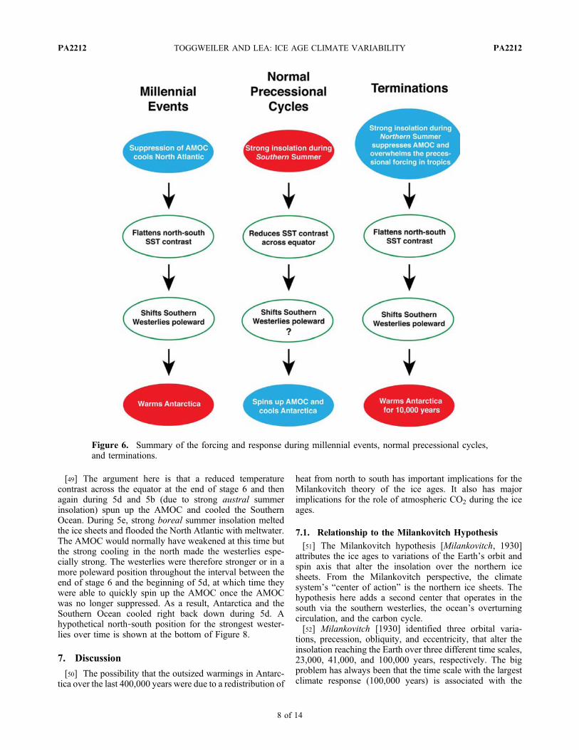
then produces an extraordinary change in the southernwesterlies, which leads to an extraordinary increase inupwelling that one sees directly in the opal accumulationaround Antarctica [Anderson et al., 2009]. The shift in thewesterlies melts back the sea ice and warms the oceanaround Antarctica and causes a lot of CO2 to be released upto the atmosphere at the same time. In this way, the e peaksseen in the Antarctic ice cores are a direct reflection of theextraordinary melting and cooling that took place around theNorth Atlantic in response to the strong summer insolationin the Northern Hemisphere.[41] This concept is summarized in Figure 6, which

summarizes the forcing and response during millennialevents, precessional cycles, and terminations. The phases ofthe three factors have been set so that each factor gives riseto a reduced SST contrast between the hemispheres.[42] First, consider Figure 6 (middle), which describes the

forcing and response when the insolation during northernsummers is at a minimum and the insolation during southernsummers is at a maximum. This describes the situationbefore and after the e intervals. The insolation forcing in thiscase spins up the AMOC (red circulation) and helps coolAntarctica by transporting southern heat into the NorthernHemisphere.[43] Millennial events in Figure 6 (left) lead to the

opposite outcome. A cooler North Atlantic reduces the

temperature contrast between the hemispheres and shifts thesouthern westerlies poleward, but in this case the AMOC(red circulation) is actively suppressed by the freshwatercoming into the North Atlantic. So, the poleward shiftedwesterlies spin up the blue circulation instead. The oceanaround Antarctica warms, Antarctica warms, and CO2 fromthe blue domain is vented up to the atmosphere.[44] Terminations (Figure 6, right) are basically giant

millennial events that are forced by precession. A key ele-ment of our hypothesis is that the freshening and cooling ofthe North Atlantic is so great at these times that it over-whelms the normal response from the precessional forcing.Thus, the temperature contrast between the hemispheres isreduced instead of enhanced and the southern westerliesshift toward Antarctica rather than away from Antarctica.[45] Strong evidence in support of this hypothesis was

compiled years ago by Crowley [1992]. Figure 7 (top) [fromCrowley, 1992, Figure 7]. It compares SSTs from the sub-antarctic zone of the Southern Ocean with SSTs from theNorth Atlantic during the latter part of stage 6 and the firstpart of stage 5. SSTs in the Southern Ocean reach theirinterglacial maximum at 130 kyr B.P. at the same time thatSSTs in the North Atlantic hit their minimum. Thus, theentire interval of southern warming takes place while theNorth Atlantic is cooling. The cooling in the NorthAtlantic, meanwhile, occurs while the insolation duringnorthern summers is ramping up from its minimum about140,000 years ago to its maximum about 128,000 years ago.[46] In Figure 7 (bottom), a proxy for the strength of the

AMOC (in the sense of Lisiecki et al. [2008]) is added,which shows that the middepth d13C reaches its minimumvalue with respect to the rest of the ocean at the same timethat the North Atlantic was coldest and Antarctica waswarmest [Mix and Fairbanks, 1985]. Similar informationfrom the North Atlantic appears in the work by Oppo et al.[1997].[47] Crowley interpreted these changes in terms of the

AMOC switching off and on. He assumed that higher levelsof atmospheric CO2 caused the warming in the south, and hewas most interested in using the suppression of the AMOCbefore 130 kyr and the spin up of the AMOC after 130 kyrto explain the delayed warming in the north. We argue herethat the southern westerlies shifted toward Antarctica whenthe summer insolation began melting back the northern icesheets just after 135 kyr. The poleward shifted westerliesthen warmed the south and brought about the CO2 increase.The CO2 increase was therefore a consequence of themechanism that warmed Antarctica and was not the cause ofthe warming.[48] This hypothesis can also explain why Antarctica and

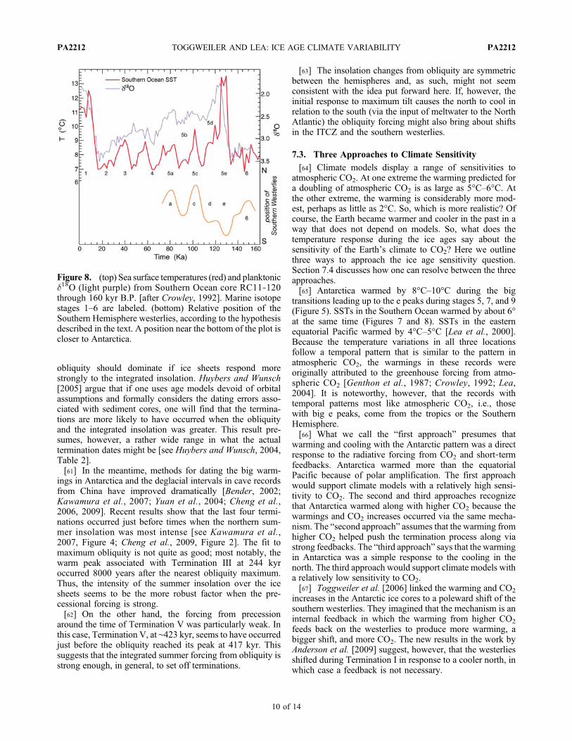
the Southern Ocean warm and cool in such an extreme waybefore, during, and after terminations. Figure 8 [also fromCrowley, 1992] compares SST and d18O records fromRC11‐120, the Southern Ocean core used in Figure 7. TheSST record from RC11‐120 is noteworthy for its intense butbrief interglacials that are limited to stages 1, 5e, and 7e[Hays et al., 1976; Imbrie et al., 1992]. The brief inter-glacials show that the Southern Ocean warmed dramaticallyduring 5e but then cooled off again almost as dramaticallyduring 5d.


7 of 14

[49] The argument here is that a reduced temperaturecontrast across the equator at the end of stage 6 and thenagain during 5d and 5b (due to strong austral summerinsolation) spun up the AMOC and cooled the SouthernOcean. During 5e, strong boreal summer insolation meltedthe ice sheets and flooded the North Atlantic with meltwater.The AMOC would normally have weakened at this time butthe strong cooling in the north made the westerlies espe-cially strong. The westerlies were therefore stronger or in amore poleward position throughout the interval between theend of stage 6 and the beginning of 5d, at which time theywere able to quickly spin up the AMOC once the AMOCwas no longer suppressed. As a result, Antarctica and theSouthern Ocean cooled right back down during 5d. Ahypothetical north‐south position for the strongest wester-lies over time is shown at the bottom of Figure 8.

7. Discussion

[50] The possibility that the outsized warmings in Antarc-tica over the last 400,000 years were due to a redistribution of

heat from north to south has important implications for theMilankovitch theory of the ice ages. It also has majorimplications for the role of atmospheric CO2 during the iceages.

7.1. Relationship to the Milankovitch Hypothesis

[51] The Milankovitch hypothesis [Milankovitch, 1930]attributes the ice ages to variations of the Earth’s orbit andspin axis that alter the insolation over the northern icesheets. From the Milankovitch perspective, the climatesystem’s “center of action” is the northern ice sheets. Thehypothesis here adds a second center that operates in thesouth via the southern westerlies, the ocean’s overturningcirculation, and the carbon cycle.[52] Milankovitch [1930] identified three orbital varia-

tions, precession, obliquity, and eccentricity, that alter theinsolation reaching the Earth over three different time scales,23,000, 41,000, and 100,000 years, respectively. The bigproblem has always been that the time scale with the largestclimate response (100,000 years) is associated with the

Figure 6. Summary of the forcing and response during millennial events, normal precessional cycles,and terminations.


8 of 14

weakest forcing (from the eccentricity of the orbit), whilethe strongest forcing (from precession and obliquity) operatesover time scales that exhibit less climate variability [Hays etal., 1976]. The extraordinary southern warming during the epeaks is a major reason why the response over 100,000 yearsis so large.[53] Our extension to the Milankovitch hypothesis says

that orbitally induced changes in the polar north and in thetropics activate the southern center by altering the temper-ature contrast between the hemispheres. The southern centerthen makes the temperatures in Antarctica rise and fall alongwith the level of atmospheric CO2.[54] The southern center also reddens the forcing from the

north to produce more variability over 100,000 years. If thelevel of atmospheric CO2 responded only to the westerlies, itwould rise and fall back in the sameway that the temperaturesin Antarctica fall back after the e peaks in Figure 5. But thelevel of CO2 does not fall back in the same way, as it lagsbehind the temperature changes, especially after the e peaks.

This is because the venting of CO2 from the deep ocean up tothe atmosphere brings about massive changes in the burial ofCaCO3 that boost the overall CO2 response and redden itsvariability out to a longer time scale [Broecker and Peng,1987; Toggweiler, 2008].[55] According to Toggweiler [2008], the CaCO3 effect on

atmospheric CO2 has an internal time scale that is similar to,but independent of, the eccentricity time scale. As such, thevariability in the south operates in the same frequency bandas the modulation of the precessional cycle (via the eccen-tricity cycle). The oceanic CO2 system “learns” about thisaspect of the orbital forcing through its response to themelting during the first strong precessional cycle.[56] These complementary time scales allow the northern

ice sheets and the oceanic CO2 system to generate a com-plementary kind of variability in each other: lower CO2

helps make the ice sheets very large over 50,000 years at atime when the Earth’s orbit is more circular and the pre-cessional forcing is weak (in the sense of Hays et al. [1976]and Shackleton [2000]), and the extraordinary input ofmeltwater from the large ice sheets causes CO2 to be ventedup to the atmosphere when the precessional forcing becomesstrong again.[57] Our sense is that neither of these quantities, ice volume

or CO2, would exhibit much 100,000 year variabilitywithout the variability of the other. The venting of CO2 upto the atmosphere needs the meltwater from large ice sheets,and large ice sheets need a reddened CO2 time scale thatcan keep atmospheric CO2 low for 50,000 years. The100,000 year cycle is a phenomenon that developed when theice sheets and CO2 system began “talking” back and forthover their common time scale.

7.2. Role of Obliquity

[58] Millennial events were not part of the originalMilankovitch hypothesis but are invoked by Anderson et al.[2009] to help explain Termination I. The claim made hereis that terminations are giant millennial events forced byprecession. This argument works best as an explanation forTerminations II, III, and IV, which occurred during timeswhen the precessional forcing was particularly strong, butmakes less sense for Terminations I and V when the preces-sional forcing was not very strong. To be more complete, theargument needs to incorporate the tilt (obliquity) of theEarth’s axis.[59] The tilt of the Earth’s axis is greater around the last

five terminations in a way that would have produced warmsummers in the vicinity of the northern ice sheets at roughlythe right times. This led Huybers [2006] to argue thatobliquity is, in fact, more important during the ice ages thanprecession. According to Huybers and Wunsch [2005],precession appears to be more important only because thechronologies in marine d18O records were tuned to maxi-mize responses in the precession and eccentricity bands.[60] The critical distinction is whether ice sheets respond

more strongly to the intensity of the summer insolation orthe insolation integrated over the summer season [Huybers,2006]. The forcing from precession should dominate if icesheets respond more strongly to the intensity of the insola-tion around the summer solstice, while the forcing from

Figure 7. (top) Comparison of northern and southern seasurface temperatures during marine isotope stages 5d and5e and the last part of stage 6 [after Crowley, 1992]. Theplot shows SSTs from North Atlantic core V30‐97 (boldblue curve) (41°N) [CLIMAP Project Members, 1984] andSSTs from Southern Ocean core RC11‐120 (red curve) (44°S)[Hays et al., 1976]. (bottom) The d13C difference (bold greencurve) between V30‐97 (North Atlantic) and V19‐30 (easternequatorial Pacific) has been added as a measure of NADWstrength [Mix and Fairbanks, 1985].


9 of 14

obliquity should dominate if ice sheets respond morestrongly to the integrated insolation. Huybers and Wunsch[2005] argue that if one uses age models devoid of orbitalassumptions and formally considers the dating errors asso-ciated with sediment cores, one will find that the termina-tions are more likely to have occurred when the obliquityand the integrated insolation was greater. This result pre-sumes, however, a rather wide range in what the actualtermination dates might be [see Huybers and Wunsch, 2004,Table 2].[61] In the meantime, methods for dating the big warm-

ings in Antarctica and the deglacial intervals in cave recordsfrom China have improved dramatically [Bender, 2002;Kawamura et al., 2007; Yuan et al., 2004; Cheng et al.,2006, 2009]. Recent results show that the last four termi-nations occurred just before times when the northern sum-mer insolation was most intense [see Kawamura et al.,2007, Figure 4; Cheng et al., 2009, Figure 2]. The fit tomaximum obliquity is not quite as good; most notably, thewarm peak associated with Termination III at 244 kyroccurred 8000 years after the nearest obliquity maximum.Thus, the intensity of the summer insolation over the icesheets seems to be the more robust factor when the pre-cessional forcing is strong.[62] On the other hand, the forcing from precession

around the time of Termination V was particularly weak. Inthis case, Termination V, at ∼423 kyr, seems to have occurredjust before the obliquity reached its peak at 417 kyr. Thissuggests that the integrated summer forcing from obliquity isstrong enough, in general, to set off terminations.

[63] The insolation changes from obliquity are symmetricbetween the hemispheres and, as such, might not seemconsistent with the idea put forward here. If, however, theinitial response to maximum tilt causes the north to cool inrelation to the south (via the input of meltwater to the NorthAtlantic) the obliquity forcing might also bring about shiftsin the ITCZ and the southern westerlies.

7.3. Three Approaches to Climate Sensitivity

[64] Climate models display a range of sensitivities toatmospheric CO2. At one extreme the warming predicted fora doubling of atmospheric CO2 is as large as 5°C–6°C. Atthe other extreme, the warming is considerably more mod-est, perhaps as little as 2°C. So, which is more realistic? Ofcourse, the Earth became warmer and cooler in the past in away that does not depend on models. So, what does thetemperature response during the ice ages say about thesensitivity of the Earth’s climate to CO2? Here we outlinethree ways to approach the ice age sensitivity question.Section 7.4 discusses how one can resolve between the threeapproaches.[65] Antarctica warmed by 8°C–10°C during the big

transitions leading up to the e peaks during stages 5, 7, and 9(Figure 5). SSTs in the Southern Ocean warmed by about 6°at the same time (Figures 7 and 8). SSTs in the easternequatorial Pacific warmed by 4°C–5°C [Lea et al., 2000].Because the temperature variations in all three locationsfollow a temporal pattern that is similar to the pattern inatmospheric CO2, the warmings in these records wereoriginally attributed to the greenhouse forcing from atmo-spheric CO2 [Genthon et al., 1987; Crowley, 1992; Lea,2004]. It is noteworthy, however, that the records withtemporal patterns most like atmospheric CO2, i.e., thosewith big e peaks, come from the tropics or the SouthernHemisphere.[66] What we call the “first approach” presumes that

warming and cooling with the Antarctic pattern was a directresponse to the radiative forcing from CO2 and short‐termfeedbacks. Antarctica warmed more than the equatorialPacific because of polar amplification. The first approachwould support climate models with a relatively high sensi-tivity to CO2. The second and third approaches recognizethat Antarctica warmed along with higher CO2 because thewarmings and CO2 increases occurred via the same mecha-nism. The “second approach” assumes that the warming fromhigher CO2 helped push the termination process along viastrong feedbacks. The “third approach” says that the warmingin Antarctica was a simple response to the cooling in thenorth. The third approach would support climate models witha relatively low sensitivity to CO2.[67] Toggweiler et al. [2006] linked the warming and CO2

increases in the Antarctic ice cores to a poleward shift of thesouthern westerlies. They imagined that the mechanism is aninternal feedback in which the warming from higher CO2

feeds back on the westerlies to produce more warming, abigger shift, and more CO2. The new results in the work byAnderson et al. [2009] suggest, however, that the westerliesshifted during Termination I in response to a cooler north, inwhich case a feedback is not necessary.

Figure 8. (top) Sea surface temperatures (red) and planktonicd18O (light purple) from Southern Ocean core RC11‐120through 160 kyr B.P. [after Crowley, 1992]. Marine isotopestages 1–6 are labeled. (bottom) Relative position of theSouthern Hemisphere westerlies, according to the hypothesisdescribed in the text. A position near the bottom of the plot iscloser to Antarctica.


10 of 14

[68] New observations by Cheng et al. [2009] show thatnorthern cooling and ITCZ shifts also occurred duringTerminations II, III, and IV. This is seen in a series of d18Oanomalies in cave records from central China, which Chenget al. [2009] call Weak Monsoon Intervals (WMIs). TheWMIs are very well dated and are found to be contempo-raneous with the warmings in Antarctica and rising CO2.[69] The melting history of the northern ice sheets is

recorded in the d18O variations in deep‐sea cores, which arenot very well dated. Given the strong link between theWMIs and northern cooling during Terminations I–IV,Cheng et al. [2009] shift the chronology for core ODP 980from the North Atlantic [McManus et al., 1999] so that ice‐rafted debris (IRD) in the core during Termination II linesup with WMI II in China. This is important because the IRDin ODP 980 is found within the same interval in which thebenthic d18O in the core is falling toward its interglacialvalues. Cheng et al.’s [2009] modified chronology puts themidpoint of Termination II at 133 kyr, a time when thesummer insolation over the ice sheets was only halfway toits maximum level. The modified chronology also makes themelting of the northern ice sheets contemporaneous with thewarmings and the CO2 increases in the south.[70] The Cheng et al. [2009] chronology makes a strong

statement in support of the second approach, in whichwarming from higher CO2 helps push the termination pro-cess along via strong feedbacks. It is at variance with tra-ditional thinking (and the basis for the original chronologyfor core ODP 980), which puts Termination II at 128 kyr B.P.when the summer insolation was at its peak. The insolationis not as strong at 133 kyr as it is at 128 kyr. So, a termi-nation at 133 kyr requires atmospheric CO2 to do more ofthe work. Cheng et al. [2009, p. 252] conclude that “risinginsolation and rising CO2, generated with multiple positivefeedbacks, drove the termination.”[71] Cheng et al.’s [2009] early termination date implies

that relatively small increases in atmospheric CO2 generatedenough warming to be instrumental in melting back thenorthern ice sheets and, through the melting, were able topush the CO2 mechanism along in the south. This seemsproblematic: how can higher CO2 be critical in melting backthe northern ice sheets and be caused by the melting at thesame time? Can the feedback possibly be this strong?[72] The mechanism outlined in this paper lends itself to

the third approach. From this perspective, the two hemi-spheres are fundamentally out of synch. The brief warmintervals in Antarctica during Terminations II, III, and IVare not interglacials in the usual sense. Rather they are de-glacial intervals that develop when the orbital forcing be-gins melting the ice sheets in the north. The cooling in thenorth and the displacement of heat from north to southaccount for all the warming in Antarctica during the bigtransitions. Atmospheric CO2 is critical in melting back theice sheets after the level of CO2 has reached its peak, notbefore.[73] From this perspective, atmospheric CO2 is important

mainly because of the duration of its cycle. According toRoe [2006], the precession of the Earth’s axis generates thelargest insolation anomalies and has the biggest impact on

the ice sheets. These anomalies, however, can only act onthe ice sheets for 10,000 years at a time. The forcing due toCO2 is weak in comparison, but a low level of atmosphericCO2 had 40,000–50,000 years to operate on the ice sheetsduring the second halves of the longer cycles. The Earthcooled during the ice ages mainly via the albedo effect ofthe northern ice sheets, which was brought about, in part,by the sustained low level of CO2 during the second halvesof the longer cycles.

7.4. Fates of the Three Approaches

[74] The increases in atmospheric CO2 during the bigtransitions in Antarctica are known to lag several hundredyears behind the warmings [Fischer et al., 1999; Caillon etal., 2003]. This is a big problem for the first approach abovebecause higher CO2 cannot be the cause of the warmings ifit lags behind. Proponents of the first approach are leftarguing that the error on the lag is large enough that the leadmight be zero [Hansen et al., 2007]. Of equal significance isthe fact that the brief warm intervals in Antarctica duringTerminations II, III, and IV are more sharply peaked in timethan the CO2 peaks. This is a problem for both the first andsecond approaches because the observed CO2 variations,such as they are, cannot give rise to warmings that are moresharply peaked. It makes more sense to say that the warmpeaks were caused in their entirety by something else.[75] Logic aside, the fate of the third approach rests ulti-

mately with the melting chronology. If the northern icesheets had indeed melted back halfway by 133 kyr, asargued by Cheng et al. [2009], the third approach, theapproach put forward here, is clearly wrong.[76] The question is: how does one anchor the chronology

of the d18O records in marine sediments? Cheng et al.[2009] do it by linking the IRD in ODP 980 to the WMIsin China. We would do it differently. Marine records fromthe tropics and Southern Hemisphere have well defined SSTmaxima that occur thousands of years before the minima ind18O in the same cores (Figure 8) [Lea et al., 2000; Barrowset al., 2007]. We would anchor these SST maxima to thewarm peaks in Antarctica. The WMIs in China come to anend at the same time as the warm peaks in Antarctica and so,by our estimation, the WMIs come to an end along with thewarm southern SSTs. The minima in oceanic d18O thencome along thousands of years later. This means that thenorthern ice sheets continued to melt for thousands of yearsafter the WMIs, as one would expect from the traditionalchronology for ODP 980.[77] This is the pattern seen during Termination I, which

is absolutely dated. WMI I lasts from 17.5 to 10.6 kyr[Cheng et al., 2009]; Antarctica is warmest at 11 ky[Kawamura et al., 2007]; Southern Ocean and tropicalPacific SSTs are warmest between 10 and 11 kyr[Labracherie et al., 1989; Stott et al., 2004]; and thenorthern ice sheets disappear by 6–7 kyr, 4000–5000 yearslater [Lambeck and Chappell, 2001]. The sea level high-stand at the end of the Termination II has also been inde-pendently dated at 122 to 115 kyr (Figure 5) [Thompson andGoldstein, 2005]. A highstand at this time is consistent withthe assumptions here and the traditional termination date of128 kyr.


11 of 14

[78] It seems to us that the meltwater that produced theWMIs came from the initial melting of the northern icesheets. The combination of a suppressed AMOC and icesheets that were still very large gave rise to the sea ice coverover the North Atlantic that produced the extraordinarynorthern cooling and the WMIs. The northern cooling andthe WMIs ended about halfway through the terminationswhen the ice sheets had become smaller and the warmingfrom atmospheric CO2 was at a maximum.[79] Temperature changes in the topics offer another

objective way to assess the climate sensitivity. SSTs in thetropical Indian and Pacific Oceans typically increase byabout 3°C between the LGM and late Holocene (as seen incore 806B in the work by Lea et al. [2000] and in the worksby Stott et al. [2002], Visser et al. [2003], Saraswat et al.[2005], Stott et al. [2007], and Xu et al. [2008]). Threedegrees is a fair amount of warming for a 100 ppm CO2

increase [Broccoli and Manabe, 1987]. Given the remote-ness of these areas from the northern ice sheets, however,most of the 3° warming might conceivably be due to higherCO2.[80] In this regard, the 4°–5° warming in TR163‐19 from

the eastern equatorial Pacific [Lea et al., 2000] is atypical.Yet, the SST record from TR163‐19 has prominent e peaksand, as such, is highly correlated in time with atmosphericCO2 [Lea, 2004]. We would argue that the extra warmingand the SST‐CO2 correlation in TR163‐19 make sense:shifts of the ITCZ have a particularly large effect on SSTs inthe eastern equatorial Pacific, and shifts of the ITCZ are partof the mechanism that makes atmospheric CO2 go up anddown [Anderson et al., 2009]. Thus, much of the 4°–5°warming, like the warming in Antarctica, can be explainedby a north‐south displacement of the ITCZ.[81] The best measure of the warming due to CO2 should

be the portion of the glacial‐interglacial SST change that iscommon to the whole region. The compilation of PacificSST records by Tachikawa et al. [2009] shows that SSTsbegan rising earlier south of the equator than north of theequator. Thus, Tachikawa et al.’s intratropical differencessuggest that much of the 3° warming in the tropics was not

due to CO2 [Stott et al., 2007]. They lend support instead tothe idea that the two hemispheres were out of synch.

8. Conclusions

[82] The whole Earth did not warm and cool togetherduring the big transitions of the ice ages. The south warmed,in particular, while the north remained cold. The north alsobecame very cold toward the ends of the glacial stages longafter the south had reached its glacial minimum. The bigtransitions took place when a resurgent precessional cycleproduced inputs of meltwater to the North Atlantic thatlasted for thousands of years. The meltwater inputs suppressedthe AMOC, flattened the temperature contrast between thehemispheres, and produced a redistribution of heat from northto south that warmed Antarctica and the Southern Ocean. Thesame factors caused the level of CO2 in the atmosphere to risealong with the temperatures in Antarctica.[83] Atmospheric CO2 was important during the ice ages

because it varied with such a long time scale. The long timescale allowed the oceanic CO2 system and northern icesheets to interact in ways that gave rise to large temperaturechanges in the Earth’s polar regions. The long time scalealso allowed the variability in northern ice volume toenhance the variability in atmospheric CO2, and vice versa.Without the long time scale for CO2, the overall level ofclimate variability during the ice ages would have beenmuch smaller.

[84] Acknowledgments. The work of Nick Shackleton (1937–2006)foreshadows much of what is presented here. His insight was to see that theNorthern and Southern Hemispheres and atmospheric CO2 contributed tothe distinctive 100,000 year variability in marine d18O records in differentways [Shackleton, 2000]. Although largely unappreciated, subsequent icecore records and sea level reconstructions have supported his view. For allthe dedication and painstaking attention to detail that led him to find andput forward this perspective, the authors would like to dedicate this paper toNick Shackleton. The authors would like to acknowledge Dick Wetheraldand Eric Galbraith for their internal reviews of the original manuscript.Frank Lamy, Lorraine Lisiecki, Valerie Masson‐Delmotte, George Denton,and Jeff Severinghaus also made valuable suggestions. The authors wouldalso like to thank Peter Huybers for his formal reviews and for his inputregarding the obliquity cycle.

ReferencesAhn, J., and E. J. Brook (2007), AtmosphericCO2 and climate from 65 to 30 ka B.P., Geo-phys. Res. Lett., 34, L10703, doi:10.1029/2007GL029551.

Ahn, J., and E. J. Brook (2008), AtmosphericCO2 and climate on millennial time scalesduring the last glacial period, Science, 322,83–85, doi:10.1126/science.1160832.

Anderson, R. F., S. Ali, L. Bradtmiller, M. Q.Fleisher, and L. H. Burckle (2009), Wind‐driven upwelling in the Southern Ocean andthe deglacial rise of atmospheric CO2, Science,323, 1443–1448, doi:10.1126/science.1167441.

Barrows, T. T., S. Juggins, P. De Deckker,E. Calvo, and C. Pelejero (2007), Long‐termsea surface temperature and climate changein the Australian–New Zealand region, Paleo-ceanography, 22, PA2215, doi:10.1029/2006PA001328.

Bender, M. L. (2002), Orbital tuning chronologyfor the Vostok climate record supported bytrapped gas composition, Earth Planet. Sci.

Lett., 204, 275–289, doi:10.1016/S0012-821X(02)00980-9.

Bintanja, R., R. S.W. van deWal, and J. Oerlemans(2005), Modelled atmospheric temperaturesand global sea levels over the past million years,Na tu r e , 437 , 125–128 , do i : 10 . 1038 /nature03975.

Blunier, T., and E. J. Brook (2001), Timing ofmillennial‐scale climate change in Antarcticaand Greenland during the last glacial period,Science, 291, 109–112, doi:10.1126/science.291.5501.109.

Blunier, T., et al. (1998), Asynchrony of Antarcticand Greenland climate change during the lastglac ia l per iod, Nature , 394 , 739–743,doi:10.1038/29447.

Bond, G., W. Broecker, S. Johnsen, J. McManus,L. Labeyrie, J. Jouzel, and G. Bonani (1993),Correlations between climate records fromNorth Atlantic sediments and Greenland ice,Nature, 365, 143–147, doi:10.1038/365143a0.

Broccoli, A. J., and S. Manabe (1987), The influ-ence of continental ice, atmospheric CO2, andland albedo on the climate of the Last GlacialMaximum, Clim. Dyn., 1, 87–99, doi:10.1007/BF01054478.

Broecker, W. S. (1998), Paleocean circulationduring the last deglaciation: A bipolar see-saw?, Paleoceanography, 13(2), 119–121,doi:10.1029/97PA03707.

Broecker, W. S., and T.‐H. Peng (1987), Therole of CaCO3 compensation in the glacial‐interglacial atmospheric CO2 change, GlobalB i o g e o c h em . C y c l e s , 1 ( 1 ) , 1 5 – 2 9 ,doi:10.1029/GB001i001p00015.

Broecker, W. S., and J. van Donk (1970), Inso-lation changes, ice volumes, and the 18Orecord in deep‐sea cores, Rev. Geophys., 8,169–198, doi:10.1029/RG008i001p00169.

Caillon, N., et al. (2003), Timing of atmosphericCO2 and Antarctic temperature changes acrossTermination III, Science, 299, 1728–1731,doi:10.1126/science.1078758.


12 of 14

Cheng, H., et al. (2006), A penultimate glacialmonsoon record from Hulu Cave and two‐phase glacial terminations, Geology, 34(3),217–220, doi:10.1130/G22289.1.

Cheng, H., et al. (2009), Ice age terminations,Science, 326, 248–252, doi:10.1126/science.1177840.

CLIMAP Project Members (1984), The lastinterglacial ocean, Quat. Res., 21, 123–224.

Crowley, T. J. (1992), North Atlantic DeepWater cools the Southern Hemisphere, Paleo-ceanography, 7(4), 489–497, doi:10.1029/92PA01058.

Denton, G. H., R. B. Alley, G. C. Comer, andW. S. Broecker (2005), The role of seasonalityin abrupt climate change, Quat. Sci. Rev., 24,1159–1182, doi:10.1016/j.quascirev.2004.12.002.

EPICA Community Members (2006), One‐to‐one coupling of glacial climate variabilityin Greenland and Antarctica, Nature, 444,195–198, doi:10.1038/nature05301.

Fischer, H., et al. (1999), Ice core records ofatmospheric CO2 around the last three glacialterminations, Science , 283 , 1712–1714,doi:10.1126/science.283.5408.1712.

Genthon, G., J.M. Barnola, D. Raynaud, C. Lorius,J. Jouzel, N. I. Barkov, Y. S. Korotkevich, andV. M. Kotlyakov (1987), Vostok ice core:Climate response to CO2 and orbital forcingchanges over the last climate cycle, Nature,329, 414–418, doi:10.1038/329414a0.

Hansen, J., M. Sato, P. Kharecha, G. Russell,D. W. Lea, and M. Siddall (2007), Climatechange and trace gases, Philos. Trans. R.Soc. Ser. A, 365, 1925–1954, doi:10.1098/rsta.2007.2052.

Haug, G., K. A. Hughen, D. M. Sigman, L. C.Peterson, and U. Röhl (2001), Southwardmigration of the Intertropical ConvergenceZone through the Holocene, Science, 293,1304–1308, doi:10.1126/science.1059725.

Hays, J. D., J. Imbrie, and N. J. Shackleton(1976), Variations in the Earth’s orbit: Pace-maker of the ice ages, Science, 194, 1121–1132, doi:10.1126/science.194.4270.1121.

Huybers, P. (2006), Early Pleistocene glacialcycles and the integrated summer insolationforcing, Science, 313, 508–511, doi:10.1126/science.1125249.

Huybers, P., and G. Denton (2008), Antarctictemperature at orbital time scales controlledby local summer duration, Nat. Geosci., 1,787–792, doi:10.1038/ngeo311.

Huybers, P., and C. Wunsch (2004), A depth‐derived Pleistocene age model: Uncertaintyestimates, sedimentation variability, and non-linear climate change, Paleoceanography, 19,PA1028, doi:10.1029/2002PA000857.

Huybers, P., and C. Wunsch (2005), Obliquitypacing of the late Pleistocene glacial termina-tions, Nature, 434, 491–494, doi:10.1038/nature03401.

Imbrie, J., et al. (1992), On the structure andorigin of major glaciation cycles: 1. Linearresponses to Milankovitch forcing, Paleocea-nography, 7(6), 701–738, doi:10.1029/92PA02253.

Indermühle, A., E. Monnin, B. Stauffer, T. F.Stocker, and M. Wahlen (2000), AtmosphericCO2 concentrations from 60 to 20 kyr BP fromthe Taylor Dome ice core, Antarctica, Geo-p h y s . R e s . L e t t . , 2 7 ( 5 ) , 7 3 5 – 7 3 8 ,doi:10.1029/1999GL010960.

Ito, T., and M. J. Follows (2005), Preformedphosphate, soft tissue pump and atmospheric

CO 2 , J . M a r . R e s . , 6 3 , 8 1 3 – 8 3 9 ,doi:10.1357/0022240054663231.

Kaiser, J., F. Lamy, and D. Hebbeln (2005), A70‐kyr sea surface temperature record offsouthern Chile (Ocean Drilling Program Site1233), Paleoceanography, 20, PA4009,doi:10.1029/2005PA001146.

Kawamura, K., et al. (2007), Northern Hemi-sphere forcing of climate cycles in Antarcticaover the past 360,000 years, Nature, 448,912–916, doi:10.1038/nature06015.

Labracherie, M., D. Labeyrie, J. Duprat, E. Bard,M. Arnold, J.‐J. Pichon, and J.‐C. Duplessy(1989), The last deglaciation in the SouthernOcean, Paleoceanography, 4(6), 629–638,doi:10.1029/PA004i006p00629.

Lambeck, K., and J. Chappell (2001), Sea levelchange through the last glacial cycle, Science,292, 679–686, doi:10.1126/science.1059549.

Lamy, F., J. Kaiser, H. W. Arz, D. Hebbeln,U. Ninnemann, O. Timm, A. Timmermann,and J. R. Toggweiler (2007), Modulation ofthe bipolar seesaw in the Southeast Pacificduring Termination 1, Earth Planet. Sci. Lett.,259, 400–413, doi:10.1016/j.epsl.2007.04.040.

Lea, D. W. (2004), The 100,000‐yr cycle in tropo-spheric SST, greenhouse forcing, and climate sen-sitivity, J. Clim., 17, 2170–2179, doi:10.1175/1520-0442(2004)017<2170:TYCITS>2.0.CO;2.

Lea, D.W., D. K. Pak, andH. J. Spero (2000), Cli-mate impact of Late Quaternary equatorialPacific sea surface temperature variations,Science, 289, 1719–1724, doi:10.1126/science.289.5485.1719.

Lea, D. W., D. K. Park, L. C. Peterson, and K. A.Hughen (2003), Synchroneity of tropical andhigh‐latitude Atlantic temperatures over the lastglacial termination, Science, 301, 1361–1364,doi:10.1126/science.1088470.

Levitus, S. (1982), Climatological atlas of theworld ocean, NOAA Prof. Pap. 13, 173 pp.,U.S. Gov. Print. Off., Washington, D. C.

Lisiecki, L. E., M. E. Raymo, and W. B. Curry(2008), Atlantic overturning responses to latePleistocene climate forcings, Nature, 456,85–88, doi:10.1038/nature07425.

Lorius, C., J. Jouzel, D. Raynaud, J. Hansen, andH. Le Treut (1990), The ice core record: Cli-mate sensitivity and future greenhouse warm-ing, Nature, 347, 139–145, doi:10.1038/347139a0.

McManus, J. F., D. W. Oppo, and J. L. Cullen(1999), A 0.5‐million‐year record ofmillennial‐scale climate variability in the NorthAtlantic, Science, 283, 971–975, doi:10.1126/science.283.5404.971.

Milankovitch, M. (1930), Mathematische Klima-lehre und Astronomische Theorie der Klimasch-wankungen, 176 pp., Gebruder Borntraeger,Berlin.

Mix, A. C., and R. G. Fairbanks (1985), NorthAtlantic surface‐ocean control of Pleistocenedeep‐ocean circulation, Earth Planet. Sci.Lett., 73, 231–243, doi:10.1016/0012-821X(85)90072-X.

Monnin, E., et al. (2001), Atmospheric CO2concentrations over the last glacial termina-tion, Science, 291, 112–114, doi:10.1126/science.291.5501.112.

Oppo, D. W., M. Horowitz, and S. J. Lehman(1997), Marine core evidence for reduced deepwater production during Termination II fol-lowed by a relatively stable substage 5e (Ee-mian), Paleoceanography, 12(1), 51–63,doi:10.1029/96PA03133.

Peterson, L. C., G. H. Haug, K. A. Hughen, andU. Röhl (2000), Rapid changes in the hydro-logic cycle of the tropical Atlantic during thelast glacial , Science , 290 , 1947–1951,doi:10.1126/science.290.5498.1947.

Petit, J. R., et al. (1999), Climate and atmo-spheric history of the past 420,000 years fromthe Vostok ice core, Antarctica, Nature, 399,429–436, doi:10.1038/20859.

Roe, G. (2006), In defense of Milankovitch, Geo-phys. Res. Lett., 33, L24703, doi:10.1029/2006GL027817.

Saraswat, R., R. Nigam, S.Weldeab, A.Mackensen,and P. D. Naidu (2005), A first look at past seasurface temperatures in the equatorial IndianOcean from Mg/Ca in foraminifera, Geophys.Res . Le t t . , 32 , L24605 , do i :10 .1029 /2005GL024093.

Shackleton, N. J. (2000), The 100,000‐yr cycleidentified and found to lag temperature, carbondioxide, and orbital eccentricity, Science, 289,1897–1902, doi:10.1126/science.289.5486.1897.

Siegenthaler, U., et al. (2005), Stable carboncycle‐climate relationship during the latePleistocene, Science , 310 , 1313–1317,doi:10.1126/science.1120130.

Stott, L., C. Poulsen, S. Lund, and R. Thunell(2002), Super ENSO and global climate oscil-lations at millennial time scales, Science, 297,222–226, doi:10.1126/science.1071627.

Stott, L., et al. (2004), Decline of surface temper-ature and salinity in the western tropicalPacific Ocean in the Holocene epoch, Nature,431, 56–59, doi:10.1038/nature02903.

Stott, L., A. Timmermann, and R. Thunell(2007), Southern Hemisphere and deep‐seawarming led deglacial atmospheric CO2 riseand tropical warming, Science, 318, 435–438, doi:10.1126/science.1143791.

Tachikawa, K., L. Vidal, C. Sonzogni, andE. Bard (2009), Glacial/interglacial sea surfacetemperature changes in the southwest Pacificover the last 360 ka, Quat. Sci. Rev., 28,1160–1170.

Thompson, W. G., and S. L. Goldstein (2005),Open system coral ages reveal persistent sub-orbital sea‐level cycles, Science, 308, 401–404, doi:10.1126/science.1104035.

Timmermann, A., S. J. Lorenz, S.‐I. An,A. Clement, and S.‐P. Xie (2007), Effect oforbital forcing on the mean climate and vari-ability of the tropical Pacific, J. Clim., 20,4147–4159, doi:10.1175/JCLI4240.1.

Timmermann, A., O. Timm, L. Stott, andL. Menviel (2009), The roles of CO2 and orbitalforcing in driving Southern Hemispheric tem-perature variations during the last 21,000 yr,J. Clim. , 22 , 1626–1640, doi:10.1175/2008JCLI2161.1.

Toggweiler, J. R. (2008), Origin of the 100,000‐yrtimescale in Antarctic temperatures and atmo-spheric CO2, Paleoceanography, 23, PA2211,doi:10.1029/2006PA001405.

Toggweiler, J. R., and H. Bjornsson (2000), DrakePassage and paleoclimate, J. Quat. Sci., 15(4),319–328, doi:10.1002/1099-1417(200005)15:4<319::AID-JQS545>3.0.CO;2-C.

Toggweiler, J. R., and B. Samuels (1995), Effectof Drake Passage on the global thermohalinecirculation, Deep Sea Res., Part I, 42(4), 477–500, doi:10.1016/0967-0637(95)00012-U.

Toggweiler, J. R., J. L. Russell, and S. R. Carson(2006), Midlatitude westerlies, atmosphericCO2, and climate change during the ice ages,


13 of 14

Paleoceanography, 21, PA2005, doi:10.1029/2005PA001154.

Tzedakis, P. C., K. H. Roucoux, L. de Abreu,and N. J. Shackleton (2004), Duration of foreststages in southern Europe and interglacial cli-mate variability, Science, 306, 2231–2235,doi:10.1126/science.1102398.

Visser, K., R. Thunnell, and L. Stott (2003),Magnitude and timing of temperature changein the Indo‐Pacific warm pool during deglaci-ation, Nature, 421, 152–155, doi:10.1038/nature01297.

Waelbroeck, C., et al. (2002), Sea‐level anddeep water temperature changes derived from

benthic foraminifera isotopic records, Quat.Sci. Rev., 21, 295–305, doi:10.1016/S0277-3791(01)00101-9.

Wang, X., A. S. Auler, R. L. Edwards, H. Cheng,E. Ito, and M. Solheid (2006), Interhemisphericanti‐phasing of rainfall during the last glacialperiod, Quat. Sci. Rev., 25 , 3391–3403,doi:10.1016/j.quascirev.2006.02.009.

Xu, J., A. Holbourn, W. Kuhnt, Z. Jian, andH. Kawamura (2008), Changes in the thermo-cline structure of the Indonesian outflow duringTerminations I and II, Earth Planet. Sci. Lett.,273, 152–162, doi:10.1016/j.epsl.2008.06.029.

Yuan, D., et al. (2004), Timing, duration, andtransitions of the last interglacialAsianmonsoon,Science, 304, 575–578, doi:10.1126/science.1091220.

D. W. Lea, Department of Earth Science,University of California, Santa Barbara, CA93106, USA. ([email protected])J. R. Toggweiler, Geophysical Fluid Dynamics

Laboratory, NOAA, PO Box 308, Princeton, NJ08542, USA. ([email protected])


14 of 14

Documents

Temperature differences between the hemispheres and ice age