Embed Size (px)
Citation preview

Study of 34mCl beam production at the National Superconducting Cyclotron Laboratory.
By
Olalekan Abdulqudus Shehu
Approved by:
Benjamin Crider (Major Professor)Jeff Allen WingerDipangkar Dutta
Henk F. Arnoldus (Graduate Coordinator)Rick Travis (Dean, College of Arts & Sciences)
A ThesisSubmitted to the Faculty ofMississippi State University
in Partial Fulfillment of the Requirementsfor the Degree of Master of Science
in Nuclear Physicsin the Department of Physics and Astronomy
Mississippi State, Mississippi
August 2020

ProQuest Number:
All rights reserved
INFORMATION TO ALL USERSThe quality of this reproduction is dependent on the quality of the copy submitted.
In the unlikely event that the author did not send a complete manuscript and there are missing pages, these will be noted. Also, if material had to be removed,
a note will indicate the deletion.
Published by ProQuest LLC (
ProQuest
). Copyright of the Dissertation is held by the Author.
All Rights Reserved.This work is protected against unauthorized copying under Title 17, United States Code
Microform Edition © ProQuest LLC.
ProQuest LLC789 East Eisenhower Parkway
P.O. Box 1346Ann Arbor, MI 48106 - 1346
28028510
28028510
2020

Copyright by
Olalekan Abdulqudus Shehu
2020

Name: Olalekan Abdulqudus Shehu
Date of Degree: August 7, 2020
Institution: Mississippi State University
Major Field: Nuclear Physics
Major Professor: Benjamin Crider
Title of Study: Study of 34mCl beam production at the National Superconducting CyclotronLaboratory.
Pages of Study: 82
Candidate for Degree of Master of Science
The success ofmany experiments at rare-isotope facilities, such as theNational Superconducting
Cyclotron Laboratory (NSCL), depends on achieving a level of statistics that is partly driven by
the overall number of nuclei produced in the beam. One such future study at the NSCL requires
maximizing the beam content of 34mCl. To prepare for this 34mCl study, an initial measurement
to determine the 34mCl yields and overall beam purity was performed at the NSCL by utilizing
a V-decay experimental station. Isotopes delivered to the experimental station were identified
using standard time of flight and energy loss techniques. To explore ways of maximizing 34mCl
production, 6 different beam energy settings that selected different rigidities for isotopic selection
and altered its entrance angles before the beamwent into the fragment separator, were utilized. The
absolute intensity of the peak energies associated with the decay of 34mCl (1177, 2127, and 3304
keV) were determined, as well as the overall number of 34Cl atoms delivered, thereby enabling
34mCl yield and beam purity determinations for each beam setting.

Key words: V decay, isomeric state, W rays

DEDICATION
This thesis is dedicated to my parents Mr. Usman Shehu and Mrs. Nimot Shehu.
ii

ACKNOWLEDGEMENTS
First, I would like to thank my advisor, Dr. Benjamin Crider, for his guidance and support
over the past two years and for facilitating my participation in many experiments, particularly this
project. His mentorship throughout my graduate studies at the Mississippi State University has
helped me position myself in line with what I hope to accomplish in the long run, including the
next chapter of my career. His approachability and availability, despite numerous commitments
made it easy for me to focus and work efficiently while balancing my coursework and research. It
has been an absolute joy working with you. Thank you.
I would also like to acknowledge my guidance thesis committee, Dr. Jeff Allen Winger and Dr.
Dipangkar Dutta for their advice, input and availability.
I wish to express my gratitude to Calem Hoffman and Tom Ginter at the National Supercon-
ducting Cyclotron Laboratory (NSCL) for providing essential information and direction pertaining
to my analysis as well as giving inputs to my thesis.
I also want to thank the National Science Foundation (NSF) for providing the financial support
to carryout this work. This work was supported by the National Science Foundation under Grant
No. PHY 1848177 (CAREER).
I would like to give a special thanks to Timilehin Ogunbeku for being a friend and an available
member of my research group despite his relocation to Michigan. His courteous and friendly
nature made my settling down in the Mississippi State University environment an easy one. I
iii

appreciate your reassuring words when I was discouraged and your assistance in obtaining some
of the results presented in this thesis. I also wish to thank Yongchi Xiao for his tremendous help in
the completion of my analysis. This thesis would be incomplete without both their contributions.
I would be remiss to not acknowledge my fellow graduate students, Daniel Solomon Araya,
Sapan Luitel, Udeshika Perera and Nuwan Chaminda. I really did enjoy our hangouts and long
talks and I am grateful for the camaraderie among us. I truly value our friendship and it has been a
pleasure meeting you all. I wish to thank Daniel Solomon Araya in particular, for a friendship that
has helped me through all my exams and for being the best office mate. He provided me with sage
advice and direction. Thank you.
Finally, my heartfelt thanks to my parents and siblings, for their incessant love, encouraging
words and prayers.
iv

TABLE OF CONTENTS
DEDICATION . . . . . . . . . . . . . . . . . . . . . . . . . . . . . . . . . . . . . . . . ii
ACKNOWLEDGEMENTS . . . . . . . . . . . . . . . . . . . . . . . . . . . . . . . . . . iii
LIST OF TABLES . . . . . . . . . . . . . . . . . . . . . . . . . . . . . . . . . . . . . . vii
LIST OF FIGURES . . . . . . . . . . . . . . . . . . . . . . . . . . . . . . . . . . . . . . viii
LIST OF SYMBOLS, ABBREVIATIONS, AND NOMENCLATURE . . . . . . . . . . . xi
CHAPTER
I. INTRODUCTION . . . . . . . . . . . . . . . . . . . . . . . . . . . . . . . . . . 1
1.1 The atomic nucleus . . . . . . . . . . . . . . . . . . . . . . . . . . . . . 11.2 Binding energy . . . . . . . . . . . . . . . . . . . . . . . . . . . . . . . 21.3 The nuclear shell model . . . . . . . . . . . . . . . . . . . . . . . . . . 31.4 Nuclear deformation . . . . . . . . . . . . . . . . . . . . . . . . . . . . 81.5 Goals of the experiment . . . . . . . . . . . . . . . . . . . . . . . . . . 9
II. RADIOACTIVE DECAY . . . . . . . . . . . . . . . . . . . . . . . . . . . . . . 11
2.1 Radioactive decay law . . . . . . . . . . . . . . . . . . . . . . . . . . . 112.2 V decay . . . . . . . . . . . . . . . . . . . . . . . . . . . . . . . . . . . 13
2.2.1 V+ decay . . . . . . . . . . . . . . . . . . . . . . . . . . . . . . . 142.2.2 V- decay . . . . . . . . . . . . . . . . . . . . . . . . . . . . . . . 152.2.3 Electron capture . . . . . . . . . . . . . . . . . . . . . . . . . . . 15
2.3 V-decay selection rules . . . . . . . . . . . . . . . . . . . . . . . . . . . 162.4 W-ray decay . . . . . . . . . . . . . . . . . . . . . . . . . . . . . . . . . 192.5 W-ray interaction with matter . . . . . . . . . . . . . . . . . . . . . . . . 20
2.5.1 Photoelectric absorption . . . . . . . . . . . . . . . . . . . . . . 202.5.2 Compton scattering . . . . . . . . . . . . . . . . . . . . . . . . . 212.5.3 Pair production . . . . . . . . . . . . . . . . . . . . . . . . . . . 22
2.6 Internal conversion . . . . . . . . . . . . . . . . . . . . . . . . . . . . . 232.7 Bateman equations . . . . . . . . . . . . . . . . . . . . . . . . . . . . . 24
v

III. FACILITIESAND INFRASTRUCTUREFORPERFORMINGE16032AEXPER-IMENT . . . . . . . . . . . . . . . . . . . . . . . . . . . . . . . . . . . . . . . 26
3.1 National Superconducting Cyclotron Laboratory (NSCL) . . . . . . . . . 263.2 Cyclotrons . . . . . . . . . . . . . . . . . . . . . . . . . . . . . . . . . 27
3.2.1 Cyclotron radiofrequency (RF) . . . . . . . . . . . . . . . . . . . 283.2.2 Coupled Cyclotron Facility . . . . . . . . . . . . . . . . . . . . . 29
3.3 Primary beam and reaction target . . . . . . . . . . . . . . . . . . . . . 303.3.1 Fragmentation process for producing exotic nuclei with large N/Z
ratio . . . . . . . . . . . . . . . . . . . . . . . . . . . . . . . . . 313.4 A1900 fragment separator . . . . . . . . . . . . . . . . . . . . . . . . . 333.5 Ion implantation into a CeBr3 scintillator . . . . . . . . . . . . . . . . . 363.6 Segmented Germanium Array (SeGA) detector . . . . . . . . . . . . . . 37
IV. EXPERIMENTAL RESULTS . . . . . . . . . . . . . . . . . . . . . . . . . . . 38
4.1 The decay of 34Cl . . . . . . . . . . . . . . . . . . . . . . . . . . . . . . 384.2 Determining the amount of 34mCl in the beam . . . . . . . . . . . . . . . 41
4.2.1 Detection setup characterization . . . . . . . . . . . . . . . . . . 414.2.1.1 SeGA energy calibration . . . . . . . . . . . . . . . . . . . 424.2.1.2 SeGA Absolute Efficiency Calibration . . . . . . . . . . . 434.2.1.3 Deadtime correction . . . . . . . . . . . . . . . . . . . . . 49
4.2.2 Beam settings clarification . . . . . . . . . . . . . . . . . . . . . 494.2.3 Time cuts on SeGA spectrum . . . . . . . . . . . . . . . . . . . . 544.2.4 Branching ratio and efficiency corrections. . . . . . . . . . . . . . 594.2.5 Absolute numbers of 34mCl ions implanted . . . . . . . . . . . . . 59
4.3 Identifying implanted 34Cl ions . . . . . . . . . . . . . . . . . . . . . . 624.3.1 Particle identification using ΔE and ToF information . . . . . . . . 624.3.2 Determining time of flight . . . . . . . . . . . . . . . . . . . . . 634.3.3 Determining the number of 34Cl for each beam setting . . . . . . . 634.3.4 Graphical cuts on the PID spectrum . . . . . . . . . . . . . . . . 71
4.3.4.1 Determining transmission efficiency to the CeBr3 implanta-tion detector. . . . . . . . . . . . . . . . . . . . . . . . . . 71
4.4 Isomeric ratio of 34Cl . . . . . . . . . . . . . . . . . . . . . . . . . . . . 75
V. CONCLUSION . . . . . . . . . . . . . . . . . . . . . . . . . . . . . . . . . . . 76
REFERENCES . . . . . . . . . . . . . . . . . . . . . . . . . . . . . . . . . . . . . . . . 78
vi

LIST OF TABLES
2.1 V decay selection rules for allowed and forbidden transitions . . . . . . . . . . . . 173.1 Fundamental properties of A1900 . . . . . . . . . . . . . . . . . . . . . . . . . . 344.1 Parameters used in Eq. 4.5 to calculate the W-ray detector efficiency of SeGA. . . . 494.2 Four beam setting indicating information obtained from A1900 beam line savesets.
Bd 1,2,3,4 refers to the magnetic rigidity of the D1, D2, D3 and D4 superconductingdipole magnet. D1 and D2 were set to same Bd value and D3 and D4 were set to thesame Bd value. . . . . . . . . . . . . . . . . . . . . . . . . . . . . . . . . . . . . 51
4.3 Time window for beam settings in nanoseconds. . . . . . . . . . . . . . . . . . . . 534.4 Raw W-ray peak areas for each 34mCl W ray along with W-ray detector efficiency for
all beam settings and their associated uncertainties. . . . . . . . . . . . . . . . . . 584.5 Branching ratios for the 34mCl W-ray energies . . . . . . . . . . . . . . . . . . . . 594.6 Absolute number of 34mCl determined from each W ray for all beam settings and
their associated uncertainties. These were determined using Eq. 4.8 . . . . . . . . 604.7 Weighted average number of implanted 34mCl for each beam setting and their asso-
ciated uncertainties. . . . . . . . . . . . . . . . . . . . . . . . . . . . . . . . . . 624.8 Number of 34Cl isotope implanted into CeBr3 for each beam setting. . . . . . . . . 724.9 Transmission efficiency from thefirst PINdetector to theCeBr3 implantation detector
for each beam setting. . . . . . . . . . . . . . . . . . . . . . . . . . . . . . . . . 734.10 Isomeric state content ratio of each beam setting in 34Cl. . . . . . . . . . . . . . . 75
vii

LIST OF FIGURES
1.1 (Left) First ionization energies of the atomic elements from hydrogen (Z=1) tonobelium (Z=102). (Right) Differences in neutron separation energy for even-evennuclei and their even-odd neighbors . . . . . . . . . . . . . . . . . . . . . . . . . 4
1.2 Nuclear shell structure considering the infinite well potential (Left) and harmonicoscillator potential (Right) . . . . . . . . . . . . . . . . . . . . . . . . . . . . . . 6
1.3 Wood-Saxon potential is the spectrum labeled WS. The spectrum labeled WS+LSincludes the spin-orbit term . . . . . . . . . . . . . . . . . . . . . . . . . . . . . 7
2.1 Decay rate of a nuclei as a function of its half-life . . . . . . . . . . . . . . . . . . 122.2 Compton-scattered electron energy as a function of scattering angle for several W-ray
energy . . . . . . . . . . . . . . . . . . . . . . . . . . . . . . . . . . . . . . . . . 222.3 Linear attenuation coefficient of NaI showing contributions from photoelectric ab-
sorption, Compton scattering and pair production . . . . . . . . . . . . . . . . . . 233.1 A two dee cyclotron . . . . . . . . . . . . . . . . . . . . . . . . . . . . . . . . . 273.2 Layout of the coupled cyclotron facility consisting of K500 and K1200 cyclotrons,
the A1900 fragment separator and the experimental vaults N2-N6 and S1-S3 . . . 303.3 Atomic nuclei landscape indicating stable and exotic nuclei . . . . . . . . . . . . . 323.4 Detailed picture of A1900 showing superconducting dipole magnet D1-D4 and
24 quadrupole magnets housed in 8 cryostats . . . . . . . . . . . . . . . . . . . . 333.5 Wedge degrader shown in image2. A degrader slows down the beam particles
depending on their charge and velocity differences. At the second stage, the differentisotopes are now separated . . . . . . . . . . . . . . . . . . . . . . . . . . . . . . 35
4.1 Decay scheme the of �c = 0+ ground state of 34Cl, which has an half life of 1.5266(4)s and decays to the �c = 0+ ground state of 34S with a branching ratio of 100 % . . 39
4.2 Decay scheme of 34mCl, �c = 3+, which has an half life of 31.99(3) minutes anddecays through internal transition (44.6(6)%) and V+ decay (55.4(6)%) . . . . . . . 40
4.3 Setting 1 34Cl ion normalized implantation depth distribution inside the CeBr3. . . 454.4 Setting 2 34Cl ion normalized implantation depth distribution inside the CeBr3. . . 454.5 Setting 3 34Cl ion normalized implantation depth distribution inside the CeBr3. . . 464.6 Setting 4 34Cl ion normalized implantation depth distribution inside the CeBr3. . . 464.7 Setting 5 34Cl ion normalized implantation depth distribution inside the CeBr3. . . 474.8 Setting 6 34Cl ion normalized implantation depth distribution inside the CeBr3. . . 474.9 Simulated W-ray efficiency - Setting 1-6 . . . . . . . . . . . . . . . . . . . . . . . 48
viii

4.10 (a) (Top)Plot of calibrated energy of raw events in SeGA vs the time stamp of eachevent in nanoseconds. The 6 vertically dense count area indicates that the experimentutilized 6 beam settings. (b) (Bottom)A spectrum showing counts vs time stamp ofeach event in SeGA. The red vertical lines are an indication of beam window. Forexample; the first line from the left is the beam on for the first setting, and the secondred line is the beam on for the next beam setting. . . . . . . . . . . . . . . . . . . 52
4.11 Fitted W peaks (1177 keV, 2127 keV, 3304 keV, respectively) of 34mCl for BeamSetting 1 . . . . . . . . . . . . . . . . . . . . . . . . . . . . . . . . . . . . . . . 55
4.12 Fitted W peaks (1177 keV, 2127 keV, 3304 keV, respectively) of 34mCl for BeamSetting 2 . . . . . . . . . . . . . . . . . . . . . . . . . . . . . . . . . . . . . . . 55
4.13 Fitted W peaks (1177 keV, 2127 keV, 3304 keV, respectively) of 34mCl for BeamSetting 3 . . . . . . . . . . . . . . . . . . . . . . . . . . . . . . . . . . . . . . . 56
4.14 Fitted W peaks (1177 keV, 2127 keV, 3304 keV, respectively) of 34mCl for BeamSetting 4 . . . . . . . . . . . . . . . . . . . . . . . . . . . . . . . . . . . . . . . 56
4.15 Fitted W peaks (1177 keV, 2127 keV, 3304 keV respectively) of 34mCl for Beam Setting 5 574.16 Fitted W peaks (1177 keV, 2127 keV, 3304 keV, respectively) of 34mCl for Beam
Setting 6 . . . . . . . . . . . . . . . . . . . . . . . . . . . . . . . . . . . . . . . 574.17 (a)Particle identification plot for Beam Setting 1 showing ions implanted into the
CeBr3 implantation detector. On the x-axis is the time of flight while on the y-axisis the energy loss. (b) Graphical cut used to determine the total number of 34Cl forthis setting. . . . . . . . . . . . . . . . . . . . . . . . . . . . . . . . . . . . . . . 65
4.18 (a)Particle identification plot for Beam Setting 2 showing ions implanted into theCeBr3 implantation detector. On the x-axis is the time of flight while on the y-axisis the energy loss. (b) Graphical cut used to determine the total number of 34Cl forthis setting. . . . . . . . . . . . . . . . . . . . . . . . . . . . . . . . . . . . . . . 66
4.19 (a)Particle identification plot for Beam Setting 3 showing ions implanted into theCeBr3 implantation detector. On the x-axis is the time of flight while on the y-axisis the energy loss. (b) Graphical cut used to determine the total number of 34Cl forthis setting. . . . . . . . . . . . . . . . . . . . . . . . . . . . . . . . . . . . . . . 67
4.20 (a)Particle identification plot for Beam Setting 4 showing ions implanted into theCeBr3 implantation detector. On the x-axis is the time of flight while on the y-axisis the energy loss. (b) Graphical cut used to determine the total number of 34Cl forthis setting. . . . . . . . . . . . . . . . . . . . . . . . . . . . . . . . . . . . . . . 68
4.21 (a)Particle identification plot for Beam Setting 5 showing ions implanted into theCeBr3 implantation detector. On the x-axis is the time of flight while on the y-axisis the energy loss. (b) Graphical cut used to determine the total number of 34Cl forthis setting. . . . . . . . . . . . . . . . . . . . . . . . . . . . . . . . . . . . . . . 69
4.22 (a)Particle identification plot for Beam Setting 6 showing ions implanted into theCeBr3 implantation detector. On the x-axis is the time of flight while on the y-axisis the energy loss. (b) Graphical cut used to determine the total number of 34Cl forthis setting. . . . . . . . . . . . . . . . . . . . . . . . . . . . . . . . . . . . . . . 70
ix

4.23 (a)CeBr3 implantation spectrum showing the PSPMT dynode energy. (b) PINspectrum showing the energy loss in the PIN detector. The transmission efficiencyto the implantation detector will be the ratio of number at the top right corner in (a)to the number at the top right corner in (b). . . . . . . . . . . . . . . . . . . . . . 74
x

LIST OF SYMBOLS, ABBREVIATIONS, AND NOMENCLATURE
SeGA Segmented Germanium Array
CeBr3 Cerium Bromide
NSCL National Superconducting Cyclotron Laboratory
PAC Program Advisory Committee
log 5 C Comparative half life
MeV Mega-electron volt
Z Atomic number
DC Direct current
RF Radiofrequency
CCF Coupled Cyclotron Facility
enA Electrical nano amperes
PPS Particles Per Second
PIN p-n type semiconductor
ToF Time of flight
TKE Total kinetic energy
TAC Time-to-Amplitude-Converter
PID Particle identification
PSPMT Position Sensitive Photo-Multiplier Tube
MCA Multi-channel analyzer
keV Kilo-electron volt
NIST National Institute of Standard and Technology
SRM Standard Reference Material
xi

GEANT4 Toolkit for the simulation of the passage of particles through matter
ISOL Isotope Separation On Line
xii

CHAPTER I
INTRODUCTION
1.1 The atomic nucleus
The atomic nucleus is the dense center of an atom consisting of protons and neutrons, which
make up the class of particles known as nucleons. Given that protons are positively charged, it would
seem impossible to confine any number of protons within a small volume. The electromagnetic
interaction between these positively charged particles should cause them to repel. However, there
is force that counteracts the repulsive electromagnetic interaction, thereby enabling a bound system
of nucleons to survive. This force is called the strong force [1].
The atomic nucleus was discovered in 1911 by Ernest Rutherford [2], based on Geiger-Marsden
gold foil experiment [3]. While there are nearly 300 stable nuclei, there are certain numbers of
protons and neutrons, called “magic" numbers (see Sec. 1.3), which have enhanced stability when
compared to other nearby nuclei. For a nucleus with too many neutrons or protons, excess energy
in the core of the atom gets out of balance. Atoms with such excess energy are called radionuclides
which follow some process of radioactive decay to become more stable. Radioactive decay also
know as radioactivity is the characteristic behavior of unstable nuclei spontaneously decaying to
different nuclei and emitting radiation in the form of particles or high energy photons.
The discovery of radioactivity took place over several years beginning with the detection of
X-rays by Wilhelm Conrad Röentgen while conducting experiments on the effect of cathode rays.
1

He placed an experimental electric tube upon a book beneath which was a photographic plate.
Later, he used the plate in his camera and was puzzled upon developing it, to find the outline
of a key on the plate. He searched through the same book and discovered a key between the
pages. The “strange“ light from the glass tube had penetrated the pages of the book; thus, X-rays
were discovered [4]. Following the discovery of X-rays, Henri Becquerel in 1896 used natural
fluorescent minerals to study the properties of X-rays. This process involved exposing potassium
uranyl sulfate to sunlight and then placing it on a photographic plate wrapped in black paper. In
this hypothesis, he believed that the uranium will absorb the sun’s energy and then emit X-rays,
but his experiment failed due to an overcast sky in Paris. For some reason, Becquerel decided to
develop his photographic plate anyway by placing it in a dark drawer. Surprisingly, the images were
strong and clear proving that radiation was emitted from the uranium without an external source
of energy such as the sun. Becquerel had discovered radioactivity [5]. Not long after, French
physicists Pierre and Marie Curie extracted uranium from uranium ores and found the leftovers
still showed radioactivity. This led to the discovery of polonium and radium. Marie Curie coined
the term radioactivity for the spontaneous emission of ionizing rays by certain atoms. Marie and
Pierre Curie were awarded half the Nobel Prize in recognition for the joint research on radiation.
The other half was awarded to Henri Becquerel for his spontaneous radioactive discovery [6].
1.2 Binding energy
In order to quantify which nuclei decay and why, one property that can be utilized is the so-
called “binding energy“ of the nucleus. Binding energy (BE) of a nucleus is the energy required to
2

separate the nucleus of an atom into protons and neutrons. The general expression for the binding
energy requires Einstein’s famous relationship equating rest mass to energy given by
� = <22 (1.1)
where < is the rest mass and 2 is the speed of light. The rest mass is used to determine the binding
energy of a nucleus [7]. Another important quantity is the average energy used to remove a single
nucleon from a nucleus. This quantity is called the binding energy per nucleon, and is represented
by
�� =�b�
(1.2)
where �b is the binding energy and � is the number of nucleons [7].
At the nuclear level, the nuclear binding energy is the energy required to separate the components
of the nucleus by overcoming the strong nuclear force. The nuclear binding energy is given by
�b(�/ -N) = [/"H + #"n − " (�/ -N)]22 (1.3)
where / is the atomic number, "H is the mass of the hydrogen nucleus (proton), # is the neutron
number, "n is the neutron mass, " (�/-N) is the atomic mass of the given nucleus [8].
In general, for a nucleus to be bound, the binding energy needs to be positive according to
Eq. 1.3. The more stable a nucleus, the higher the binding energy. Radioactivity decay therefore
occurs when a more tightly bound nucleus can be obtained.
1.3 The nuclear shell model
In the course of the study of atomic nuclei, the idea of a shell structure began to emerge.
This shell structure is analogous to the shell structure of an electrons orbital in an atom, but also3

has several differences. One way to illustrate the shell structure phenomenon in atoms is with
ionization energy, which is the energy required to remove the most loosely bound electron. The
ionization energy as a function of atomic number, Z, exhibited discontinuities as shown in Fig. 1.1
(left). The discovery of these discontinuities proved that the atom existed in electronic shells [1].
The discontinuities emerged from the underlying shell structure. In the process of filling electrons
in orbital shells, the energy is reduced considerably when the next electron is placed in a higher
energy orbital.
Figure 1.1: (Left) First ionization energies of the atomic elements from hydrogen (Z=1) to nobelium
(Z=102). (Right) Differences in neutron separation energy for even-even nuclei and their even-odd
neighbors. Figure from Ref. [8].
In the nuclear system, trends in the nuclear mass and binding energy have proved increased
stability for nuclei associated with "magic" numbers corresponding to when the proton or neutron
number equals 2, 8, 20, 28, 50, 82 and 126. Therefore, making the nuclear shell model analogous
to the atomic shell model. These numbers led to the development of the shell model, where the
4

magic numbers corresponds to the filling of major nuclear shells [1]. To compare to the ionization
energy in atoms, we can utilize the neutron separation energy ((n), which is the energy required to
remove a single neutron from the nucleus. The neutron separation energy is defined as
(n(#) = �b(�/ -N) − �(�−1/ -N-1) = [" (�−1
/ -N-1) − " (�/ -N) + "n]22 (1.4)
Here �b(�/ -N) is represented by Eq. 1.3. Similarities between the neutron separation energy and
the atomic ionization energy are apparent due to the neutron separation energy showing periodicity,
suggesting a nuclear shell structure.
The nuclear shell structure can be corroborated by describing the even # nuclei and their # + 1
neighbors in terms of the change in (n:
4(n = (n(#) − (n(# + 1) = [" (�−1/ -N-1 + " (�−1
/ -N+1) − 2" (�/ -N))]22 (1.5)
Fig. 1.1 (Right) shows the differences in neutron separation energy for even-even nuclei and their
even-odd neighbors up to fermium (/=100). Similar to the electron ionization energy, the observed
discontinuities underscores the neutron magic numbers [8].
The ability of the nuclear shell model to describe the observed behavior depends on the choice
of the potential which confines the protons and neutrons within the nucleus. Historically, theorists
tried to reproduce the magic numbers by utilizing several mathematical formalisms [1, 8]. A
harmonic oscillator potential was first considered. Solving the Schrödinger equation describes the
energy levels of a harmonic oscillator potential as shown in Fig. 1.2 (Right). The lowest shell
closures at 2, 8, and 20 were reproduced correctly by the harmonic oscillator potential but the
higher level shell closures were in disagreement. This is because it had an unrealistic potential (V
5

→ ∞) at the boundary of the nucleus [1]. Similar issues come up when considering the infinite
well potential (see Fig. 1.2) (Left).
Figure 1.2: Nuclear shell structure considering the infinite well potential (Left) and harmonic
oscillator potential (Right). Figure from Ref. [1].
The Woods-Saxon potential was considered next because it provides a much better approxima-
tion at A = ' (nucleons near the surface of a nucleus). It takes the form
+ (A) = −+0
1 + exp[ (A−')0]
(1.6)
where A is the distance from the center of the nucleus, ' is the mean nuclear radius (1.25 fm
A1/3), 0 is the surface thickness of the nucleus and +0 is the depth of the potential. Typical values
for the Wood Saxon potential depth are Vo ∼ 50 MeV. As shown in Fig. 1.3 (Left), this potential
reproduces the magic numbers 2, 8 and 20, but fails for numbers beyond.
6

Figure 1.3: Wood-Saxon potential is the spectrum labeled WS. The spectrum labeled WS+LS
includes the spin-orbit term. Figure from Ref. [9].
In the 1940’s, it was discovered that adding a spin-orbit potential to the Wood-Saxon potential
allowed the theory to reproduce all of the observed magic numbers [10, 11]. The spin-orbit
potential is represented by
+ so = + so(A)®; · ®B (1.7)
where + so(A) is a radially dependent strength constant, ®; is the orbital angular momentum and ®B is
the intrinsic nucleon spin. The term ®; · ®B describes the orbital motion and nuclear spin interactions,
and leads to a removal of the ;-degeneracy states, or a splitting of states with ;>0. This results
is shown in Fig. 1.3 (right) [1, 8]. Additionally, the spin-orbit splitting increases with angular
momentum causing the higher- 9 state to be pushed into a group of states from a lower shell. This
is how the higher magic numbers are obtained.
7

From Fig. 1.3, the 2S+1Lj spectroscopic notation is used to describe the energy levels where S
is the spin, L is the orbital angular momentum and j is the total angular momentum. The number
of nucleons a shell can hold is 2j+1. For example, 0P3/2 has a spin of -1/2, has a L=1, and a total
of 4 nucleons. The sd region adds 6, 4, 2 number of nucleons respectively to the existing magic
number of 8. Following this filling, there is a shell gap before moving into the fp region. The fp
region begins its filling with 8 nucleons, therefore leaving a shell gap. Finally the fp shell fills up
with a 4, 6, 2 nucleon numbers corresponding to 1P3/2, 0f5/2, and 1P1/2. The isotope of interest
34Cl, which has 17 protons and 17 neutrons, would have its ground state in the fp region.
1.4 Nuclear deformation
Nuclear deformation is a central concept to understanding nuclear structure [12]. Since an
understanding about the forces that shape the nucleus is incomplete, no theory has succeeded
to explain the properties of the nuclear structure wholly. Nuclear deformation depends on the
Coulomb force, the nuclear force and the shell effects. The atomic nucleus exhibits spherical,
quadrupole and higher-order multipole deformations [13].
Nuclei having deformation generally are classified into prolate, oblate, and triaxial. Prolate and
oblate nuclei are axially symmetric. This means the appearance is unchanged if rotated around an
axis. If the third axis of the nucleus is longer than the others, the nucleus is prolate and if it is
shorter, the nucleus is oblate. All three axes are different for triaxial nuclei [13].
The deformation of a nucleus impacts many observables. Beyond direct effects of impacting
level energies and transition strengthswithin excited states of a nucleus, deformation can also impact
cross-sections relevant to astrophysical processes such as the rapid proton capture nucleosynthesis
8
process which will be defined later in Sec. 1.5. One example is the enhancement of (n, W) cross
sections for many nuclei on the s-process and r-process path due to dipole deformation that can
affect the overall trajectory of these processes [14].
1.5 Goals of the experiment
The physics motivation of the experiment 16032A is to study the 34mCl yields and overall beam
purity at the NSCL. The application of this knowledge will be used for an experiment in studying
the single-neutron occupancies of the excitation energies between analog states of mirror nuclei
(atomic nuclei that contains a number of protons and a number of neutron that are interchanged)
which is called the Mirror Energy Difference (MED). MED’s probe the charge independence and
symmetry of nuclear strong force. This measurement will be focused on the high MEDs states of
35Cl and 35Ar. The states of interest can be populated with an high probability by adding a neutron
into the isomeric state of 34Cl. 34g,mCl (3,?W) reaction is further required to populate the states
of interest. The 34g,mCl (3,?W) reaction begins with a 34Cl beam hitting a deuterium (Proton +
neutron) target. This results in a 36Ar compound nucleus for a very brief amount of time(∼ 10−22
s). Then the 36Ar emits a proton and W-ray energies and the final reaction is left with the 35Cl
isotope. The isomeric state of 34Cl, which has Jc = 3+, is required to enhance the probability for
the population of the higher spin 35Cl excited states of interest and this thesis aims to measure the
isomeric state yield in a beam of 34Cl produced at the NSCL.
The study of 34Cl also plays an important role in the rp-process (rapid-proton capture) nucle-
osynthesis. The rp-process nucleosynthesis is the process responsible for the generation of many
heavy elements present in the universe. The rp-process consists of consecutive proton capture
9

onto seed nuclei to produce heavier elements [15]. Uncertainties in the rates for both the ground
and isomeric state of 34Cl, translate into uncertainties in 34S production which is an important
observable in preosolar grains. Presolar grains are solid grains that started at a time before the sun
was formed. The majority of these grains are condensed in the outflow of asymptotic giant branch
stars and supernovae [16].
An interesting feature of 34Cl is that it has a low-lying, long-lived isomer, which can complicate
its interpreted impact in the aforementioned applications. This isomer, typically labeled as 34mCl
(denoting its characterization as a "meta-stable" state) behaves differently from other isotopes in
astrophysical environments. Specifically, the assumption of thermal equilibrium in computing the
temperature-dependent V-decay rates can fail below certain temperatures [17]. Therefore, the study
of the nuclear structure of 34Cl is crucial in understanding the nuclear reaction codes to calculate
the nucleosynthesis that occurs in hot stellar environments.
10
CHAPTER II
RADIOACTIVE DECAY
There are different forms by which nuclei emit radiation to remove excess energy. The types
that are primarily relevant to the nuclei of interest in this work will be discussed here: V decay and
W decay. This chapter also goes into details about the physics governing the decay law, selection
rules and the Bateman equation.
2.1 Radioactive decay law
A universal law that describes the statistical behavior of a large number of unstable nuclei is
called the radioactive decay law. For an unstable nucleus to release particles, they must overcome
the strong nuclear force holding the nucleons together. This implies that the rate of decay varies
for different nuclei, which depends on the properties of these individual nuclei such as the number
of nucleons, the filling of shells and subshells, and the energy difference between the initial and
final states, to name a few.
The radioactive decay law states that the probability per unit time that a decay occurs in the
nucleus is a constant denoted by _, and it is independent of time. Considering # to be the total
number of nuclei in a sample and 3# to be the change in number of nuclei in the sample in a time
3C. The rate at which radioactive nuclei decay is proportional to the decay constant and can be
written as
11
3#
3C= −_# (2.1)
The constant _ varies amongst different nuclei thereby causing different observed decay rates.
Solving this first-order differential equation yields the number of nuclei # , at time C, which is an
exponential function in time given by
# (C) = #0 exp -_t (2.2)
where #0 is the number of nuclei at time C=0. Eq. 2.2 is the law of radioactive decay.
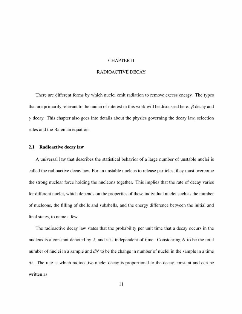
Radioactive decay can also be measured in terms of the half-life. An isotope’s half-life is the
time required for the number of atoms in a radioactive isotope to decay into half its initial value.
Fig. 2.1 shows a theoretical graph of the number of nuclei present as a function of time.
Figure 2.1: Decay rate of a nuclei as a function of its half-life. Figure from Ref. [18].
12
As shown in Fig. 2.1, the number of nuclei that has not yet decayed diminishes with the number
of half-life’s that passes. Depending on the decay mode and the relative competition between
available decay modes, half-life’s can range from approximately 10−15 seconds to many times
the age of the universe (double V decay has half-life’s on the order of 1024 years or more). The
relationship between half-life and the decay constant _, is given by
)1/2 =ln 2_
(2.3)
Another common way to refer to radioactive decay is using activity, which is the disintegration
per second of an unstable nuclei. The activity does not depend on the type of decay, but it depends
on the number of decays per second. The units are given by:
• Becquerel : 1Bq = 1 disintegration per second.
• Curie : 1Ci = 3.7 × 10¹⁰ Bq.
• Rutherford : 106 nuclei decays per second.
Activity is just the rate of decay, Eq. 2.1 can be combined with the radioactive decay law to
express the activity as
�(C) = _# (C) = �0 exp -_t (2.4)
Activity is proportional to the number of radioactive nuclei and inversely proportional to the
half-life.
2.2 V decay
V decay occurs when a neutron transforms into a proton or vice-verse. During this process the
mass number remains unchanged but the atomic number changes. There are three distinct V decay
13

processes called V+, V- and Electron Capture (EC). In general, these three processes transmute
more exotic parent nuclei to less exotic daughter nuclei.
2.2.1 V+ decay
In V+ decay, a proton-rich nucleus converts a proton into a neutron by emitting a positron (V+)
and an electron neutrino (Ee) [19]:
�/X# → �
/−1 Y#+1 + V+ + Ee +&V+ (2.5)
The &V+ energy value of this reaction is given by
&V+ = [" (�, /) − " (�, / − 1) − 2<e]22 (2.6)
where " (�, /) is the mass of the nucleus with � nucleons and / protons, <e is the mass of the
electron and 2 is the speed of light. According to Eq. 2.6, the total energy is shared between the
positron, neutrino, and the recoiling daughter nucleus. It also requires that the mass difference
between the parent and the daughter nucleus must be greater than 2me22 = 1.022 MeV [19] for V+
decay to occur. Since positron decay requires energy, it cannot occur in an isolated proton because
the mass of the neutron is greater than the mass of the proton. Additionally, because the positron
does not exist for a long period of time in the presence of matter, it interacts with an electron in
its surrounding environment leading to annihilation. The masses of both positron and electron
convert to electromagnetic energy forming two 511-keV W rays in opposite directions [20]. Typical
values for QV+ are ∼ 2 MeV - 4 MeV [19].
14

2.2.2 V- decay
In V- decay, a neutron-rich nucleus converts a neutron into proton by emitting an electron (V-)
and an electron antineutrino (Ee) [19]:
�/X# → �
/+1 Y#−1 + V- + Ee +&V- (2.7)
The &V- energy value of this reaction is given by
&V- = [" (�, /) − " (�, / + 1)]22 (2.8)
The decay energy is shared between the electron, antineutrino and the recoiling daughter nucleus.
The antineutrino like the neutrino, has no charge or significant mass, and does not readily interact
with matter. Similarly, the total energy released is the difference between the excitation energies
of the initial and final states. Typical values for Eq. 2.8 near stability is ∼0.5 MeV - 2 MeV [19].
2.2.3 Electron capture
Electron capture is like V+ decay in the sense that a proton captures an atomic electron, typically
from the innermost shell or K shell:
�/X# + 4- → �
/−1 Y#+1 + Ee +&EC (2.9)
The &EC energy value is given by,
&EC = [" (�, /) − " (�, / − 1)]22 (2.10)
After a proton captures an electron, the electron shell is left with a vacancy and the process is
accompanied by emission of a neutrino. Electron fill the lower lying shells which leads to emission
of X-rays [20]. Depending on the final state of the daughter nucleus and the binding energy, the15

neutrino is emitted with precise energy [19], with neutrino getting approximately all of the&-value
[21]. Though it is possible that neutrinos have some mass, it is very small and has a neutral
charge. Therefore, the neutrino escapes undetected from most experimental apparatuses due to the
low weak interaction cross section; therefore, the identification of electron capture decay must be
followed by tracking the secondary emission of X-rays or Auger electrons.
In general, if &EC < 1.022 MeV (2me), V+ is not feasible, only electron capture can occur. If
QEC > 1.022 MeV (2me), both electron capture and V+ can occur. If it is a stripped nucleus (no
electrons), electron capture is impossible. If QEC < 1.022 MeV (2me) and it is a stripped nucleus,
the nucleus becomes stable and cannot decay [21].
In the process of V decay, due to the energy taken away by the neutrino, there is a continuous
energy distribution for electron or positron, depending on the reaction (&) energy. This V energy
spectrum can be described by Fermi theory of V decay. In Fermi theory
_if =2cℏ|" if |2df (2.11)
where _if is the transition probability, |" if| is the matrix element for the reaction and df is the
density of final states [22].
2.3 V-decay selection rules
Angular momentum and parity conservation has to be satisfied for a V-decay transition to take
place. This gives rise to selection rules that determine whether a particular transition between an
initial and final state, both with specified spin and parity, is allowed, and, if so, what mode of decay
is likely [23]. The two emitted particles, an electron and a neutrino, have a spin of 1/2 and carry
orbital angular momentum. The orientation of electron and neutrino plays an important role in16

the selection rules. If the spin of the two particles are antiparallel (↑↓), the coupled total spin is
(V=0. This system undergoes a Fermi decay. Whereas, when the two emitted particles are aligned
parallel (↑↑ or ↓↓), (V=1. This is called a Gamow-Teller decay.
The rules for addition of angular momentum vectors implies that
| 9N1 − 9eE | ≤ 9N2 ≤ 9N1 + 9eE (2.12)
where 9N1 is the nucleus spin before decay, 9N2 is the nucleus spin after decay and 9eE is the
combined angular momentum of electron and antineutrino [25].
From Table. 2.1, allowed V decay requires that both electron and neutrino carry no orbital
angular momentum (Δ; = 0), and has no change in nuclear parity (Δc = 0). In allowed Fermi decay,
there is no change in parity and orbital angular momentum and ΔJ = 0.
In an allowed Gamow-Teller transition, the electron and neutrino carry off a unit of angular
momentum. Thus,
9N1 = 9N2 + 1 (2.13)
Table 2.1: V decay selection rules for allowed and forbidden transitions. Table from Ref. [24].
Transition type Δc Δ; Δ J log 5 C
Superallowed No 0 0 2.9 - 3.7
Allowed No 0 0,1 4.4 - 6.0
First forbidden Yes 1 0, 1, 2 6 - 10
Second forbidden No 2 1, 2, 3 10 - 13
Third forbidden Yes 3 2, 3, 4 ≥ 15
17

| �N2 − 1 |≥ �N1 ≥| �N2 + 1 | −→ Δ� = 0, 1 (2.14)
Similarly, there is no change in parity between final and initial state. The majority of transitions
are mixed Fermi and Gamow-Teller decays, since Δ� = 0 is allowed in both Fermi and Gamow
Teller allowed transition. In the special case when there is a transition from a spin 0+ state to spin
0+ state (�N1 = �N2 = 0), only Fermi decay is possible and it is called a "superallowed" V decay
[25]. The ground state of the nucleus of interest, 34Cl, follows a supperallowed V decay into the
ground state of 34S.
Allowed V decay is prohibited when the initial and final states have opposite parities. However,
such decays can occur with less probability compared to allowed V decay. These are called
forbidden transition type (Δ; ≥ 0) [19]. The degree of forbiddingness is dependent on Δ;. Decays
of Δ;=1 are called first forbidden decays, second forbidden decays has Δ;=2 [25]. Table. 2.1
summarizes the selection rules for forbidden and allowed V decay transitions.
The log 5 C value, also termed the comparative half-life, is a method for comparing the V decay
probabilities in different nuclei. The log 5 C value can also represent differences between the final
and initial state. Approximate values of log 5 V- can be calculated from
log 5 V- = 4.0 log �max + 0.78 + 0.02/ − 0.005(/ − 1);>6�max (2.15)
where �max is the energy difference inMeV of the mother and daughter final state in atomic number
/ of the V daughter [26]. The C in log 5 C is the partial half life for the decay to a specific state in
the daughter nucleus. Therefore, the partial half life for decay populating a specific state 8 in the
daughter is given by [27]
)1/2partial, i =
)1/2total
�'i(2.16)
18

where �'i is the branching ratio to the daughter state i. This ratio defines the constant rate for a
particular decay branch to the total set of possible decay branches.
2.4 W-ray decay
When a nucleus is in an excited state, it can release the energy in the form of electromagnetic
radiation (photon) in a process called W-ray decay. This energy ranges from keV to MeV. During
this decay process, there is no change in the proton number and mass number. Most V decays are
accompanied by a W ray because the daughter nucleus is left in an excited state. The level schemes
and interconnecting transitions of a radionuclide can be identified by using W-ray spectroscopy.
Similar to a V decay, the conservation of angular momentum has to be taken into consideration
in a W-ray decay process. The initial and final states have a definite angular momentum and parity.
Thus, the angular momentum (!) carried by the photon ranges from
| (� i − �f) |ℏ ≤ ! ≤ (� i + �f)ℏ → ! = ;ℏ → ; ≥ 1 (2.17)
where � i and �f are initial and final nuclear spins respectively [19].
In addition to a change in angular momentum, a change in parity between the initial and final
states will be associated with a W-ray transition. For an electric type transition the change in parity
is
Δc = (−1); (2.18)
while for a magnetic transition the change in parity is
Δc = (−1);−1 (2.19)
19

While W rays have an intrinsic spin of one (Δ; ≥ 1), some transitions are forbidden (Δ; = 0) like the
decay from 0+→0+.
2.5 W-ray interaction with matter
A study of interaction of W rays with matter is necessary to understand what reactions occur
in a detector after a decay. There are 3 major types of W-ray interactions with matter; namely the
photoelectric absorption, Compton scattering and pair production.
2.5.1 Photoelectric absorption
The photoelectric absorption involves the interaction of a W ray with an inner shell electron.
The W ray interacts with the electron in such a way that all its energy is transferred to the electron,
and thus the W-ray energy is fully absorbed. The majority of the W-ray energy is transfered to the
freed electron as kinetic energy while some is used to overcome the binding energy of the electron.
The energy of the released photoelectron �e is given by
�e = �W − �b (2.20)
where �W is W-ray energy and �b is electron binding energy. A small amount of recoil energy
remains with the atom to conserve momentum. In a radiation detector, photoelectric absorption
results in a full energy peak because the W ray gives up all its energy [28].
The probability of photoelectric absorption depends on the atomic number of the atom, electron
binding energy, and the W-ray energy. The more tightly bound the electron, the higher the proba-
20

bility. Therefore, the K-shell electrons are mostly affected. The probability is given approximately
by
g ∼ /4
�3 (2.21)
where g is the photoelectric mass attenuation coefficient [28].
2.5.2 Compton scattering
A W-ray photon can also interact by losing part of its energy to an electron, with the remainder
of its energy emitted as a new lower energy photon. To absorb recoil energy, conservation of
momentum and energy allows only a partial transfer when the electron is not tightly bound enough.
The kinetic energy of the electron is given as:
�e = �W − �′ (2.22)
where �e is the scattered electron energy, �W is the incident W-ray energy, and �′ is the scattered
W-ray energy [28]. The scattered W-ray energy can be written as function of scattering angle and
incident W-ray energy as
�′W =�W
1 + (1 − cos \) �W<022
(2.23)
where <0c2 is the electron rest mass (511 keV) and \ is the angle between incident and scattered
W rays.
Fig. 2.2 shows Compton-scattered electron energies as a function of scattering angle and W ray
energy. The sharp discontinuity corresponds to the maximum energy that can be transfered in a
single scattering. In a detector, the detector medium stops the scattered electron and the detector
produces an output pulse that is proportional to the energy lost by the incident W ray [28].
21

Figure 2.2: Compton-scattered electron energy as a function of scattering angle for several W-ray
energy. Figure from Ref. [28].
2.5.3 Pair production
Pair production is a process by which a photon is converted to an electron-positron pair. This
event converts energy into mass using Einstein’s relation (E = mc2) because the photon has no
rest mass. Any W ray totaling at least 1.022 MeV (two electron rest masses) can appear as the
kinetic energy of the pair and the recoil emitting nucleus, with the probability for pair production
increasing significantly above 1.1 MeV as shown in Fig. 2.3.
After the photon conversion, the positron combines with a free electron and both particles
annihilate. The entire mass of these two particles is then converted into two W-ray energies of
0.511 MeV each, and these W rays may or may not escape the detector. If one or both of these two
W rays escapes the detector, given enough statistics, one can see single and double escape peaks in
the energy spectrum at 0.511 MeV and 1.022 MeV below the photopeak, respectively.
22
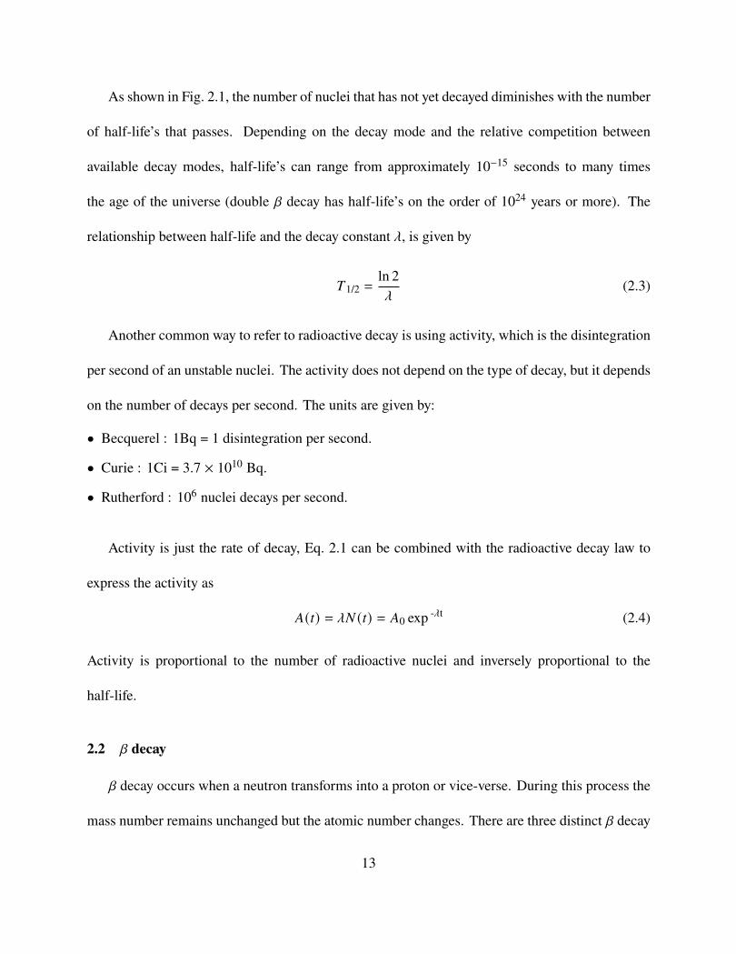
Figure 2.3: Linear attenuation coefficient of NaI showing contributions from photoelectric absorp-
tion, Compton scattering and pair production. Figure from Ref. [28].
Pair production is impossible for W-ray energies less than 1.022 MeV. The probability of pair
production is approximately proportional to the square of the atomic number [28].
2.6 Internal conversion
Internal conversion occurs when an excited nucleus interacts electromagnetically with an orbital
electron, and ejects it [8]. The vacancy created by the ejected electron is filled by an orbital electron,
which results in X-ray or Auger electron emission. The high speed electron should not be confused
with the V particle because the electron is not created during the decay process, but is a preexisting
atomic electron [29]. The kinetic energy of the emitted electron is given as
� IC = � transition − �electron binding energy (2.24)
where � transition = � i - � f is the energy difference between the initial and final state [8].
23

This mode of decay also occurs and competes with W-ray decay as a deexcitation process in
unstable nuclei. Due to this, many radioactive nuclei could emit both W rays and internal conversion
electrons. The degree to which this occurs is expressed as the total internal conversion coefficient
(U), which is the ratio of the rate of emission of internal conversion electrons to the rate of emission
of W rays:
U =#e#W
(2.25)
where #e and #W are the number of internal conversion electrons and W-ray photons, respectively,
in each time interval for a given energy decay transition. The internal conversion coefficient can
vary between 0 and∞ [29].
There is a special case of internal conversion between 0+ states called an E0 transition. In such
transitions, W rays cannot be emitted as explained in Sec. 2.4, but a transition can proceed through
internal conversion [29].
2.7 Bateman equations
The first order differential equations used in describing activities in a decay chain, based on the
initial abundance and decay rates can be described by the Bateman equations [30]. The first, or
parent, decay has its rate of decay governed by its decay constant. The second, or daughter decay,
has to then account for the growth in activity due to the decay of the parent as well as its own decay
due to its decay constant. Similar arguments are made for each subsequent member for the decay
chain. Therefore, for a series of radioactive decays of n-nuclide’s in a linear chain, the Bateman
equations are derived as
3#13C
= −_1#1 (2.26)
24

3# i3C
= _i-1# i-1 − _i# i; (8 = 2...=) (2.27)
where _i is the decay constant of the 8th nuclide. Taking into account that there are no concentrations
in all daughter nuclei at time zero, the initial conditions are specified as
#1(0) ≠ 0; # i(0) = 0; 8 > 1 (2.28)
Therefore, the nth nuclide concentration after a time C is given by the Bateman equation
#n(C) =#1(0)_n
=∑8=1
_iUi exp[−_iC] (2.29)
where
Ui =
=∏9=1; 9≠8
_j
(_j − _i)(2.30)
[30]. Eq. 2.30 can only be calculated if all decay constants are different, otherwise it goes to
infinity. The presence of infinity in the sum means it will not converge [30].
While the Bateman equations will be used in later analysis, the results of this subsequent
analysis are likely to be less precise than the results presented in this work due to needing to
develop a time binning for the fitting of our results, thereby reducing the count in our analyzed
photopeaks. The Bateman equation application to the data is left as a future project and will be
briefly described in Chapter 5.
25

CHAPTER III
FACILITIES AND INFRASTRUCTURE FOR PERFORMING E16032A EXPERIMENT
In this chapter, the experiment 16032A which was carried out at the National Superconducting
Cyclotron Laboratory (NSCL) is described. Sec. 3.1 begins with a general description of the NSCL
at Michigan State University (MSU). A description of the cyclotrons working principle is given in
Sec. 3.2. Sec. 3.3 describes the primary beam and reaction target used for isotope production. A
detailed description of the A1900 fragment separator is introduced in Sec. 3.4.
3.1 National Superconducting Cyclotron Laboratory (NSCL)
The experiment 16032A was carried out at the National Superconducting Cyclotron Labora-
tory (NSCL) at Michigan State University (MSU). The facility produces rare isotope beams at a
wide range of energies through projectile fragmentation [31, 32]. Sec. 3.3.1 discusses projectile
fragmentation in some detail. The NSCL utilizes two superconducting cyclotrons coupled together
(the K500 and the K1200), which also gives it the common name of the Coupled Cyclotron Facility
(CCF). A diverse array of experimental devices are available for conducting experiments [33].
In this experiment, a 34Cl beam was produced using an Ar16+ primary beam at 150 MeV/u via
fragmentation in an ∼1.2 mm thick Be target. The 34Cl was identified through its Time of Flight
(ToF) between a scintillator at the image 2 (i2) focal plane of the A1900 fragment separator and
26

a 65 `m Silicon PIN diode detector positioned near the experimental end station, and the energy
loss measured using the same Si PIN detector.
3.2 Cyclotrons
A cyclotron is a device that accelerates particles to high velocities using a magnetic field and
a time varying electric field. The cyclotron was originally developed by Ernest Lawrence in 1930.
Cyclotrons are generally composed of "dees", which is a set of "D" shaped hollow conductors. A
image of a two dee cyclotron is shown in Fig. 3.1.
Figure 3.1: A two dee cyclotron. Figure from Ref. [34].
To accelerate a particle, the cyclotron uses hollow metallic electrodes (dees) to which a time
varying radiofrequency (RF) electric potential is applied resulting in an electric field between the
dees in the gap. The time varying electric field accelerates the particles in the azimuthal \ direction
and the DC magnetic field bends the beam particle around a closed orbit about the I direction. The
potential changes every half a cycle as the particles move, but it is constant with respect to each
dee. Thus, the electric field inside cavity of the dee remains zero. This then requires the frequency
27

of the voltage source to be equal to the cyclotron frequency of the particle [34] as described in the
next section.
3.2.1 Cyclotron radiofrequency (RF)
Acceleration of ions is dependent on the RF potential applied to the dees [35] as mentioned
in Sec. 3.2. To derive an equation for the cyclotron frequency by looking at the interaction of a
charge particle with a magnetic field, the force on a charged particle as a result of circular motion
is considered and given by
®�mag = @ ®E× ®� (3.1)
where ®�mag is the magnetic force acting on a charged particle with charge @ moving inside a
magnetic field �. The Newton’s second law statement that describes the centripetal force that
makes the particle move in a curved path is given by
®�cent = −(<E2
A)= (3.2)
where ®�cent is the centripetal force, < is mass of the particle and = is perpendicular to the trajectory
[36]. The RF frequency is based on Eq. 3.1 and Eq. 3.2 where ®E and ®� must be perpendicular to
each other. Equating Eq. 3.1 to Eq. 3.2 gives
@ |� |<
=E
A= lRF (3.3)
Eq. 3.3 yields the magnetic field for closed orbits, where lRF is constant for a given particle.
A measure of the particle coupling strength to the magnetic field can be given by the magnetic
28
rigidity, �d, which is the magnet bending strength for a given radius and energy [37]. It is given
by:
�d =?
@=<E
@(3.4)
where ? is the momentum, @ is the charge, E is the velocity, and < is the mass . The unit for
magnetic rigidity is Tesla-meters [37].
3.2.2 Coupled Cyclotron Facility
In 1999, the NSCL upgraded to the Coupled Cyclotron Facility (CCF), see Fig. 3.2, to help
provide substantial beam intensity for ions and increased energies. Before the coupling of the
cyclotrons, the K500 and K1200 individually accelerated heavy-ion beams. The new facility
couples the K500 and K1200 to produce ion beams from Hydrogen to Uranium ranging from 200
MeV/u to 90 MeV/u [38]. The "K" in K500 and K1200 indicates the maximum kinetic energy
that a Hydrogen (proton) beam can be accelerated to in MeV. The "K" comes from multi-particle
cyclotrons where the energy from an ion of charge & and mass mo is given non-relativistically by
[39]
� = &2
�(3.5)
As shown in Fig. 3.2, the CCF houses both the K500 and K1200 cyclotrons. The basic require-
ments of the cyclotrons are to produce and transport rare isotope beams between two cyclotrons and
match six-dimensional phase space to ensure efficient injection into the K1200 cyclotron [31, 40].
The production of rare isotopes initially begins with a stable beam (like 40Ca) which is accelerated
by the K500 cyclotron to velocities of ∼0.2c.
29

Figure 3.2: Layout of the coupled cyclotron facility consisting of K500 and K1200 cyclotrons, the
A1900 fragment separator and the experimental vaults N2-N6 and S1-S3. Image from Ref. [40].
The high energy beam then passes through the K1200 cyclotron carbon stripper foil thereby
removing electrons and increasing its charge state to maximize its energy in the final stage of
acceleration. The primary beam strikes a production target, thereby resulting in the creation of
several isotope species. Before the rare isotopes are delivered into any of the 8 experimental
vaults (labeled S1-S3 and N2-N6 in Fig. 3.2), the A1900 separates incoming isotopes according to
magnetic rigidity. The A1900 fragment separator will be discussed in detail in Sec. 3.4.
3.3 Primary beam and reaction target
In the experiment 16032A carried out at NSCL, the ion of interest 34Cl, was created with a
primary beam of Ar16+ at 150 MeV/u. The Ar16+ beam was initially accelerated to 13 MeV/u in
the K500 cyclotron with a charge state of +74 and was further accelerated to 150 MeV/u in the
K1200 cyclotron with a charge state of +184. The Ar16+ beam was then fragmented by an ∼1.2mm
30

Be thick target. Beryllium is a commonly used production target due to its relatively large nuclear
number density [40].
3.3.1 Fragmentation process for producing exotic nuclei with large N/Z ratio
Exotic nuclei are short-lived nuclei that have large proton/neutron ratios as compared to the
stable nuclei found in nature. Exotic nuclei are difficult to produce and study because of the
simultaneous production of contaminant species and low production cross sections [41].
Fig. 3.3 shows the layout of the nuclear landscape in which the proton and neutron numbers are
drawn on the vertical and horizontal axis, respectively. The blue squares indicate stable isotopes
which form our universe while the yellow squares indicate the exotic nuclei which have been
observed experimentally. For the medium-mass nuclei below Z=20 and N=28, the magics numbers
are shown at 2, 8, 20 and 28. The most predominant ways of producing exotic nuclei are Isotope
Separation On Line (ISOL) and in-flight separation using heavier ions (fragmentation technique)
[42]. The latter will be discussed because of its relevance to the experiment 16032A.
In the fragmentation technique, a high energy beam is fragmented by hitting a target nucleus
which is typically 9Be. The production of exotic nuclei depends on its distance from the stability
line. The ion’s Coulomb deflection and nuclear recoil are small so that the large initial velocity
can focus all the products into a narrow cone. The mass, charge, and velocity distributions of
the products can be described by two models; namely the microscopic nucleon-nucleon scattering
model and the macroscopic abrasion framework [43].
31

Figure 3.3: Atomic nuclei landscape indicating stable and exotic nuclei. Figure adapted from
Ref. [44].
The microscopic nucleon-nucleon scattering model is best utilized for beam energies below
100 MeV/u. The microscopic nucleon-nucleon scattering model predicts many features of the
collision such as the total elastic cross-section and the mean free path of individual nucleons in
the target. Conversely, in the macroscopic abrasion framework, the target causes shearing off of
particles from the projectile nucleus, leaving the rest of the projectile to move at nearly the initial
beam velocity, carrying along some excitation energy and small downshift in velocity [43].
In the cases where the masses of the fragments are close to but smaller than that of the initial
nucleus, the fragment is maximized and the mass fragments follow an exponential decrease with
32

respect to the projectile mass number. The isotonic distribution produces neutron numbers that
are much lower than stability. Also, the isotonic distribution is almost Gaussian. Only lower mass
fragments are expected to be produced. For example, when proton-rich nuclei are close to stability,
they are best produced with the heavier N∼Z projectiles. On the other hand, neutron-rich nuclei
are produced with neutron-rich beam [43].
At the NSCL, after fragmentation, the nuclei of interest are then separated using the A1900
fragment separator.
3.4 A1900 fragment separator
The A1900 fragment separator is a high acceptance magnetic fragment separator that utilizes
four 45◦ superconducting, iron-dominated dipole magnets, labeled D1-D4 in Fig. 3.4, with a 3m
radius and 24 superconducting large-bore quadrapole magnets housed in 8 cryostat used to focus
the beam [40, 45].
Figure 3.4: Detailed picture of A1900 showing superconducting dipole magnet D1-D4 and
24 quadrupole magnets housed in 8 cryostats. Figure from Ref. [40].
The quadrupoles focus the beam in one direction, either x or y, therefore several quadrupoles
are used [45]. Table 3.1 shows the fundamental properties of the A1900 fragment separator.
33

Table 3.1: Fundamental properties of A1900. Table from Ref. [40].
Parameter A1900
Momentum acceptance (%) 5
Maximum rigidity (Tm) 6
Resolving power 2915
Dispersion (<</%) 59.5
Solid angle [msr] 8
Fig. 3.4 gives a detailed pictorial description of the A1900 fragment separator. The fragments
are initially produced after a primary beam hits a target. The mixture of primary and secondary
beams ions is then bent by the D1 and D2 dipoles to separate a secondary beam according to its
magnetic rigidity, Bd, given by Eq. 3.4. The beam components are separated by the dipoles by
choosing particles within a narrow range of magnetic rigidity [46].
Following the fragmentation filtering from D1 and D2, the ions go into image2 (Fig. 3.5).
Image2 is positioned halfway along the A1900 fragment separator where the beam is focused so
that a narrow cut can be made on the magnetic rigidity to select a subset of the fragmentation
particles in the beam. As the beam passes through image2, it becomes separated spatially based
on its Bd value.
34

Figure 3.5: Wedge degrader shown in image2. A degrader slows down the beam particles
depending on their charge and velocity differences. At the second stage, the different isotopes
are now separated. Figure from Ref. [47].
35

AnAl degrader is placed at the image2 to assist with desired isotope selection. The Al degrader
is added as a way to differentially change the velocity (rigidity) so that a second selection at the focal
plane gives further separation. As shown in Fig. 3.5, in order to keep the achromatic (colorless)
condition unchanged for the isotope of interest, the degrader is made to be wedged shape. The
wedge shape is necessary to make the beam nearly monoenergetic. The degrader is wedge shape
because the energy loss in the degrader depends on the particle velocity. The wedge is thicker
at the higher velocity end while it is thinner at the lower velocity end [46, 47]. The degrader’s
energy loss is proportional to Z2/v2, meaning energy loss depends on the different number of
protons in the ions. After the degrader, a second Bd selection occurs on ions with different Z
but similar mass-charge ratios. Then a slit with a 5% maximum acceptance is located after the
degrader to control the overall momentum acceptance X?
?[32]. The second pair of dipoles, D3
and D4, compensate for the dispersion from the first pair of dipoles, as well as the magnification
from selecting a momentum cut. The choice of primary beam, target, degrader material, degrader
thickness, and apertures in the fragment separators are parameters adjusted to control the intensity
and purity of the rare isotope beam [48].
3.5 Ion implantation into a CeBr3 scintillator
The CeBr3 implantation detector system is a fast scintillator detector with pixelated output used
in the experiment 16032A. It is capable of detecting high energy fragmentation ions, enabling
correlation of the implanted ions to subsequent decays within the detector, and provides sub-
nanosecond time resolution. The Position Sensitive Photo-Multiplier Tube (PSPMT) is coupled
to the thick CeBr3 implantation detector (49mm × 49mm × 3mm). The implantation scintillator
36

system consists of a 16 × 16 pixelated PSPMT which has 256 anodes used to determine the inter-
action position and timing between pixels, and a single dynode used for full-energy determination
and timing information.
3.6 Segmented Germanium Array (SeGA) detector
The Segmented Germanium Array (SeGA) detector is primarily used for W-ray spectroscopy
at the NSCL. Its has an excellent energy resolution for W-ray spectroscopy and it allows for
the separation of closely spaced W-ray energies. The SeGA detector detects a coincident W ray
emission if a V decay populates the daughter nucleus in an excited state. The configuration used
for the SeGA is called a "beta-SeGA" configuration which consist of two concentric rings of 8
detectors that places the CeBr3 detector at the center in order to maximize SeGA detector efficiency.
The nominal energy resolution of the SeGA detector, stated in terms of the Full Width at Half
Maximum (FWHM), is 0.13% at 662 keV and the nominal efficiency of the array in the "beta
SeGA" configuration is 4.48% at 662 keV.
37

CHAPTER IV
EXPERIMENTAL RESULTS
In this chapter, a complete analysis of the experiment 16032A is presented. The chapter begins
with the types of decay, energy levels, decay modes and decay schemes of 34Cl. The following
section goes further into determining the number of implanted 34mCl through data analysis. It then
ends on the analysis of implanted 34Cl ions and PID (Particle Identification) plots.
4.1 The decay of 34Cl
Earlier experiments have been performed on 34Cl and a great deal was previously known about
this isotope. These studies have been of paramount importance for understanding the evolution of
nuclear structure in the 34Cl region. There are two different decay possibilities in 34Cl, namely V
decay and internal transition.
The decay scheme shown in Fig. 4.1 represents the V+ decay at the �c = 0+ ground state of 34Cl,
which has a half life of 1.5266(4) s and decays to the �c = 0+ ground state of 34S with a branching
ratio of 100%. From Eq. 2.10, the Q value of this decay is 5491.634(43) keV [49, 50].
38

Figure 4.1: Decay scheme of the �c = 0+ ground state of 34Cl, which has an half life of 1.5266(4)
s and decays to the �c = 0+ ground state of 34S with a branching ratio of 100%. Figure adapted
from Ref. [49].
The decay scheme shown in Fig. 4.2 represents the evaluated data pertaining to the decay of
the �c = 3+ isomeric state of 34Cl. This state, 34mCl (see Fig. 4.2), which has a half-life of 31.99(3)
minutes, has a 44.6(6)% probability for an internal transition of EW = 146 keV to occur and a
55.4(6)% probability for a V+ decay to occur. The V+ decay results in the following three most
intense W rays in the daughter nucleus, 34S:
• 1176.650(20) keV = 2+2 → 2+1
• 2127.499(20) keV = 2+1 → 0+1
• 3304.031(20) keV = 2+2 → 0+1
39
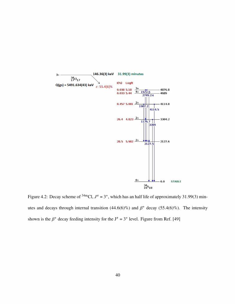
Figure 4.2: Decay scheme of 34mCl, �c = 3+, which has an half life of approximately 31.99(3) min-
utes and decays through internal transition (44.6(6)%) and V+ decay (55.4(6)%). The intensity
shown is the V+ decay feeding intensity for the Jc = 3+ level. Figure from Ref. [49]
40

These 3 intense W rays has a known absolute intensities of 14.09(24)%, 42.80(8)% and
12.29(22)% respectively [50]. All other W rays, such as 1572.57(5) keV, 1987.19(3) keV, e.t.c,
have a very small absolute intensity and the discussion on the analysis excludes them from consid-
eration towards the final results [49, 50].
Also, based on the relatively high-density of CeBr3 implantation detector when compared to
other common scintillator materials and the ongoing analysis to determining the SeGA absolute
efficiency of the 146 keV W ray energy, the remainder of this report ignores the 146-keV W ray.
4.2 Determining the amount of 34mCl in the beam
The following sections will describe efforts taken to determine the overall fraction of 34mCl in
the 34Cl beam delivered to the experimental end station. The beginning of the section discusses
ways in which the SeGA detector was calibrated in order to determine the absolute amount of
34mCl and 34Cl in the beam. The section follows up with the clarification of six beam settings used
to select 34Cl ions momentum distribution, branching ratios, and efficiency corrections.
4.2.1 Detection setup characterization
In order to determine the total number of 34mCl, the absolute number of the W rays which were
emitted by the source is needed. Hence, the number of observed W rays divide by the absolute
efficiency of the detector array is also needed. Therefore, energy and efficiency measurement
of the SeGA detectors is crucial, as well as a proper deadtime measurement. To explore ways
of maximizing 34mCl production, 6 different beam settings were utilized and the resultant W-ray
production of the delivered ions were analyzed.
41

4.2.1.1 SeGA energy calibration
The SeGA detectors shows linear response to incident W rays between tens of keV and tens
of MeV range. Therefore, it is possible to make a linear calibration using some very strong
characteristic background W rays. These W-ray energies include [51]
• 510.999(15) keV, associated with annihilation of positrons and electrons
• 788.744(8) keV, W-radiation of 138La found in LaBr3 detectors used in the setup
• 1435.795(10) keV, W-radiation of 138La found in LaBr3 detectors used in the setup
• 1460.820(5) keV, W-radiation of 40K from surroundings
When a W ray hits the detector, after the digitization and evaluation by the pixie-16 module, the
channel number of the Multi Channel Analyzer (MCA) storing the amplitude of the incident W ray
is proportional to its energy. Therefore, a linear relation between the incident W-ray energy and the
MCA channel number can be given as:
� = 0� + 1 (4.1)
where � is the W ray energy, 0 is the slope, � is the channel number storing the amplitude of the
W ray in the MCA and 1 is the intercept. The energy scale calibration for experiment 16032A was
set to 1 keV/channel.
Previous experiments calibration parameters for SeGA were initially used in the experi-
ment 16032A SeGA calibration, with the initial assumption that the physical conditions (bias
voltage, temperature, e.t.c) for operations on SeGA are the same. Therefore, we write this in the
form of
�′ = 00� + 10 (4.2)
42

where �′ is the current reading of W-ray energy. The response of SeGA experiences changes over
time because of the fluctuation of vault room temperature. Therefore, a second round of calibration
is given by the relation:
� = 01�′ + 11 (4.3)
where � is the desired reading of the W-ray energy. From Eq. 4.2 and Eq. 4.3:
� = 0100� + 0110 + 11 (4.4)
where 0 = 0100 is the slope and b = 0110 + 11 is the slope.
4.2.1.2 SeGA Absolute Efficiency Calibration
The thick CeBr3 implantation detector prevents direct measurement of the absolute efficiency
because the detector hinders the placement of National Institute of Standard and Technology
(NIST) calibrated source at the implant position. This therefore requires simulation of the actual
experimental conditions. The absolute efficiency calibration performed on SeGA further requires
extraction of relative and absolute W-ray intensities. Data were taken with a NIST-calibrated
Standard Reference Material (SRM) comprised of 125Sb, 154Eu, 155Eu [32] located on the face of
the CeBr3 (this gives the best ability to reproduce the effects of the CeBr3 crystal at least on one
side of the SeGA array). Since this source is over 20 years old, the 125Sb, which has a half-life of
2.76(25) years, has largely decayed away, leaving only 154Eu and 155Eu for use in the efficiency
determination.
A simulation was designed to replicate the material (both sensitive detector and non-sensitive
materials) as well as the geometric configuration found in our experimental setup. The simulation
was performed with the GEANT4 toolkit for the simulation of the passage of particles through43

matter. The isotropic cylindrical volume (button source) for the SRM was reproduced in the
simulation to refine the materials present for both the upstream and downstream sides of our SeGA
array in the V-SeGA configuration (8 detectors upstream and 8 detectors downstream of the thick
CeBr3 implantation scintillator). LISE++ was used [52] to determine the depth profile for the
source and implantation data in the CeBr3.
Six beam settings were utilized in the experiment 16032A, so ion implantation had to be carried
out for each settings as the implantation profiles and depth distributions informed the creation of
the volume source and its positioning inside the CeBr3 detector. Fig. 4.3 - Fig. 4.8 displays the 34Cl
ion depth distribution taken for experiment 16032A. A detailed description of the beam settings
used is described in Sec. 4.2.2. Fig. 4.3 - Fig. 4.8 were generated using the LISE++ code [32]
with parameters set to replicate the experimental beam settings while also illustrating the full 3
mm (3000 `m) thickness of the CeBr3 detector.
The efficiency simulation was run for eleven W-ray energy values ranging from 100 keV to 4000
keV with the isotropic volume source emitting one million mono-energetic W rays. The simulated
W-ray results for each beam settings is plotted on a log-log scale as shown in Fig. 4.9.
The simulated log-log scale enabled a sixth order polynomial to be used for interpolation. The
log-log fit scale is the best way of describing the simulated W-ray efficiency for ease of fitting
compatibility.
The simulated data points were fit using a linear least-squares fit to the sixth order polynomial
function of the form
� 5 5 [�W] (%) = 100 × 10[0(G)6+1(G)5+2(G)4+3 (G)3+4(G)2+ 5 (G)+6] (4.5)
44

Figure 4.3: Setting 1 34Cl ion normalized implantation depth distribution inside the CeBr3.
Figure 4.4: Setting 2 34Cl ion normalized implantation depth distribution inside the CeBr3.
45

Figure 4.5: Setting 3 34Cl ion normalized implantation depth distribution inside the CeBr3.
Figure 4.6: Setting 4 34Cl ion normalized implantation depth distribution inside the CeBr3.
46

Figure 4.7: Setting 5 34Cl ion normalized implantation depth distribution inside the CeBr3.
Figure 4.8: Setting 6 34Cl ion normalized implantation depth distribution inside the CeBr3.
47

Figure 4.9: Simulated W-ray efficiency - Setting 1-6
where G=log10(�W) and �W is the W-ray energy in keV. The resulting parameter for this six different
depth profiles are given in Table 4.1. The absolute efficiencies obtained from these fit curves for
the three W rays of interest could then be used in out analysis.
A 5% uncertainty was assigned to all efficiency calculations across each energy for all the
beam settings based on the comparison of the simulation with the SRM data because at lower
48

Table 4.1: Parameters used in Eq. 4.5 to calculate the W-ray detector efficiency of SeGA.
Parameter Setting 1 Setting 2 Setting 3 Setting 4 Setting 5 Setting 6
a 0.082342 0.077462 0.083441 0.083492 0.077335 0.078313
b -0.078313 -1.358550 -1.398310 -1.397500 -1.357770 -1.363430
c 8.915530 8.927450 8.914120 8.990000 8.920660 8.915310
d -26.211300 -26.537900 -26.143000 -26.120600 -26.527700 -26.471700
e 30.040000 29.545400 30.106400 30.445800 29.752300 29.882500
f 7.336700 11.758000 6.586340 5.202560 10.867700 10.020500
g -30.276100 -35.575300 -29.387400 -27.909800 -34.593100 -33.640100
energies, they had the largest uncertainties which is less than 5%. Therefore, a 5% uncertainty was
implemented on all parameters as a conservative approach.
4.2.1.3 Deadtime correction
Dead time is the shortest time interval between two pulses, so that both can be recorded as
separate pulses [53]. The dead-time correction was determined using internal live-time scalers,
as the ratio of accepted triggers to total triggers for each channel of the Digital Data Acquisition
System (DDAS) [32]. The count rates for different runs were low enough so that the deadtime
correction was not significant.
4.2.2 Beam settings clarification
Four A1900 settings were used to select 34Cl ions from the momentum distribution, with
two of the beam settings (Setting 5 and Setting 6) altering the angle of the beam going into the
49

A1900 fragment separator. The momentum acceptance was 0.5% in all beam settings. The 34Cl
momentum distribution settings includes
• 1st slice up: rigidity of the A1900 between the target and wedge is set at 0.75% above"LISE++ optimum"
• 1st slice down: rigidity after target is 0.75% below "LISE++ optimum"
• 2nd slice down: rigidity after target is 1.25% below "LISE++ optimum"
• 3rd slice down: rigidity after target is 1.75% below "LISE++ optimum"
"LISE++ optimum" is the rigidity value that LISE++ predicts for the peak of the fragment’s
distribution in rigidity. No measurement was taken close to "LISE++ optimum" because the
rigidity of the Ar16+ primary beam overlapped with the "LISE++ optimum" setting. The angle
measurements were made using the 1st slice up setting for the A1900. The angle on the beam was
implemented by utilizing a horizontal steering magnet and a horizontal dipole magnet between the
K1200 cyclotron and the A1900 target to put the beam at as large of a horizontal angle as allowed
by the 4-inch diameter beam pipe without losing a noticeable fraction of the beam. The beam
from the K1200 enters the A1900 target by passing roughly from west to east. A positive angle is
defined when the beam is north of the optic axis upstream from the target and south of the optic
axis downstream (east) from the target. The angle measurement is an approximate value based
on where the beam hit viewers along the beamline near the target position. Table 4.2 shows the
34Cl momentum distribution beam settings from the A1900 beam line savesets and how they were
handled within the collected experimental data set.
All beam settings of the A1900 fragment separator utilized an Ar16+ primary beam at 149.31
MeV/u and a 566.89 mg/cm2 9Be production target. Similarly, all settings used a 150 mg/cm2 Al
degrader.50

Table 4.2: Four beam setting indicating information obtained from A1900 beam line savesets. Bd
1,2,3,4 refers to the magnetic rigidity of the D1, D2, D3 and D4 superconducting dipole magnet.
D1 and D2 were set to same Bd value and D3 and D4 were set to the same Bd value.
Beam setting Setting title Bd 1,2 (Tm) Bd 3,4(Tm)
1 1st slice up 3.3484 3.2277
2 1st slice down 3.2985 3.1750
3 2nd slice down 3.2819 3.1570
4 3rd slice down 3.2653 3.1389
5 1st slice up -minus 3◦ at the A1900 target 3.3484 3.2277
6 1st slice up -plus 3◦ at the A1900 target 3.3484 3.2277
The beam setting difference can be visualized from Fig. 4.10 (a) which shows a plot of the raw
events in SeGA vs the time stamp of each event in nanoseconds. Also, projections were taken on
the SeGA time axis of Fig. 4.10 (a) to clarify the view on 6 beam settings, which is shown in Fig.
4.10 (b).
The red line on Fig. 4.10 (b) from the left indicates when the beam was turned on for the first
beam setting. In this setting, the beam rate gradually reduced. The primary beam is turned off
when a sharp drop in activity is observed. Therefore, the red vertical lines brackets the beam-on
periods. It might seem that the beam was abruptly turned on and off at the third beam setting, but
this is just an indication of drop in beam rate. The time spent in each beam setting is approximately
3.09 hrs, 1.82 hrs, 3.07 hrs, 3.67 hrs, 1.63 hrs, and 2.26 hrs respectively. Also, the binning effects
shown in Fig. 4.10(b) did not impact the final results.
51

Figure 4.10: (a) (Top)Plot of calibrated energy of raw events in SeGA vs the time stamp of each
event in nanoseconds. The 6 vertically dense count area indicates that the experiment utilized 6
beam settings. (b) (Bottom)A spectrum showing counts vs time stamp of each event in SeGA. The
red vertical lines are an indication of beam window. For example; the first line from the left is the
beam on for the first setting, and the second red line is the beam on for the next beam setting.
52

In general, the beam time on and off for each settings is shown in Table 4.3.
Table 4.3: Time window for beam settings in nanoseconds.
Beam setting 1 2 3 4 5 6
Beam on (ns) (×1013) 0.046 1.160 1.830 2.950 4.290 4.890
Beam off (ns) (×1013) 1.158 1.815 2.934 4.271 4.878 5.703
53

4.2.3 Time cuts on SeGA spectrum
Following the beam on and beam off time plot (see Fig. 4.10(b)) that indicates the different
settings used, we then projected out the W-ray singles spectra for each of the six settings, thus
allowing us to compare the results. This enabled the comparison of the W peak area corresponding
to the three primary lines from 34mCl decay for each beam setting plots showing each peak presented
in Fig. 4.11 - Fig. 4.16.
The strong 1177, 2127 and 3303-keV W rays are observed as expected. Observation of these
gamma rays indicates the presence of 34mCl in the beam. The areas of these peaks of interest were
then fitted in each spectrum, as they are the known peaks associated with 34mCl (see Fig. 4.2). A
W-ray photopeak has a shape described by a Gaussian distribution given by
5 (G) = 1f√
2cexp(−1
2( G − `f)2) (4.6)
where ` is the center of the distribution and f is the characteristic width. This Gaussian fit was
performed on top of a linear background. A single Gaussian fit has five parameters; two to describe
the linear background and three to describe the peak (a, ` and f). The number of counts is
determined using
� = 0f√
2c → f =�,�"
2√
2 ln 2(4.7)
where 0 is the height of the peak and f is the characteristic width which is related to the Full Width
at Half Maximum (FWHM).
Table 4.4 shows the W-ray peak areas for each W ray for all beam settings along with their
associated uncertainties.54

Figure 4.11: Fitted W peaks (1177 keV, 2127 keV, 3304 keV, respectively) of 34mCl for Beam Setting
1
Figure 4.12: Fitted W peaks (1177 keV, 2127 keV, 3304 keV, respectively) of 34mCl for Beam Setting
2
55

Figure 4.13: Fitted W peaks (1177 keV, 2127 keV, 3304 keV, respectively) of 34mCl for Beam Setting
3
Figure 4.14: Fitted W peaks (1177 keV, 2127 keV, 3304 keV, respectively) of 34mCl for Beam Setting
4
56

Figure 4.15: Fitted W peaks (1177 keV, 2127 keV, 3304 keV respectively) of 34mCl for Beam Setting
5
Figure 4.16: Fitted W peaks (1177 keV, 2127 keV, 3304 keV, respectively) of 34mCl for Beam Setting
6
57

Table 4.4: Raw W-ray peak areas for each 34mCl W ray along with W-ray detector efficiency for all
beam settings and their associated uncertainties.
Beam setting Energy (keV) Area (Num. of counts) Efficiency
1 1177 2.40(17) × 103 3.23(16)%
2127 5.14(12) × 103 2.28(11)%
3304 9.08(63) × 102 1.64(8)%
2 1177 3.77(16) × 103 3.22(16)%
2127 8.02(15) × 103 2.27(11)%
3304 14.20(64) × 102 1.64(8)%
3 1177 4.72(19) × 103 3.24(16)%
2127 9.73(16) × 103 2.28(11)%
3304 16.80(69) × 102 1.63(8)%
4 1177 6.45(22) × 103 3.22(16)%
2127 14.46(20) × 103 2.30(11)%
3304 26.51(89) × 102 1.64(8)%
5 1177 2.38(15) × 103 3.20(16)%
2127 4.99(12) × 103 2.27(11)%
3304 8.73(58) × 102 1.62(8)%
6 1177 3.87(18) × 103 3.20(16)%
2127 8.30(17) × 103 2.28(11)%
3304 15.46(74) × 102 1.65(8)%
58
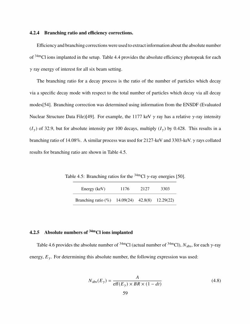
4.2.4 Branching ratio and efficiency corrections.
Efficiency and branching correctionswere used to extract information about the absolute number
of 34mCl ions implanted in the setup. Table 4.4 provides the absolute efficiency photopeak for each
W ray energy of interest for all six beam setting.
The branching ratio for a decay process is the ratio of the number of particles which decay
via a specific decay mode with respect to the total number of particles which decay via all decay
modes[54]. Branching correction was determined using information from the ENSDF (Evaluated
Nuclear Structure Data File)[49]. For example, the 1177 keV W ray has a relative W-ray intensity
(�W) of 32.9, but for absolute intensity per 100 decays, multiply (�W) by 0.428. This results in a
branching ratio of 14.08%. A similar process was used for 2127-keV and 3303-keV. W rays collated
results for branching ratio are shown in Table 4.5.
Table 4.5: Branching ratios for the 34mCl W-ray energies [50].
Energy (keV) 1176 2127 3303
Branching ratio (%) 14.09(24) 42.8(8) 12.29(22)
4.2.5 Absolute numbers of 34mCl ions implanted
Table 4.6 provides the absolute number of 34mCl (actual number of 34mCl), #abs, for each W-ray
energy, �W. For determining this absolute number, the following expression was used:
#abs(�W) =�
eff (�W) × �' × (1 − 3C)(4.8)
59

Table 4.6: Absolute number of 34mCl determined from each W ray for all beam settings and their
associated uncertainties. These were determined using Eq. 4.8
Beam setting Energy (keV) Absolute number of 34mCl in beam
1 1177 5.28(47) × 105
2127 5.26(31) × 105
3304 4.51(40) × 105
2 1177 8.31(56) × 105
2127 8.24(46) × 105
3304 7.04(49) × 105
3 1177 10.32(68) × 105
2127 9.95(55) × 105
3304 8.36(56) × 105
4 1177 14.22(89) × 105
2127 14.70(81) × 105
3304 13.13(82) × 105
5 1177 5.27(43) × 105
2127 5.13(30) × 105
3304 4.39(37) × 105
6 1177 8.60(60) × 105
2127 8.49(48) × 105
3304 7.64(55) × 105
60

where � is the observed number of counts in the W-ray singles spectrum, eff(�W) is the absolute
photopeak efficiency from Eq. 4.5, �' is the branching ratio given in Table 4.5 and 3C is the dead
time for data collection. The deadtime is ignored in this analysis (3C∼0). To determine #abs for
the 1176-keV W ray with Beam Setting 1, the number of counts in the 1176-keV peak is 2.40(17)
× 103 from Table 4.4, the absolute photopeak efficiency at 1176 keV is 3.23(16)% from Table 4.4,
the branching ratio for the 1176-keV W ray is 14.09(24)% from Table 4.5 are combined to give
#abs(1177 :4+) = 2.40(17) × 103
0.0323(16) × 0.1409(24) = 5.28(37) × 105 (4.9)
Similarly, #abs(2127 keV) for Beam Setting 1 is
#abs(2127 :4+) = 5.14(12) × 103
0.0228(11) × 0.428(8) = 5.26(14) × 105 (4.10)
Finally, #abs(3303 keV) for Beam Setting 1 is
#abs(3304 :4+) = 9.08(63) × 102
0.0164(8) × 0.1228(22) = 4.51(31) × 105 (4.11)
The same routine is followed for each of the fitted W rays, with Table 4.6 giving the results.
From Table 4.6, we can see that the results for the yield of 34mCl ions are consistent when utilizing
the 1177 keV and 2127 keV W rays. However, it is also evident that the 3304 keV W-ray provides
a systematically low absolute yield compared to the other W rays. One possible explanation is an
underestimation of its overall intensity produced from the decay of 34mCl. Despite its systematic
lower value, we still averaged it in with the other measured W-ray results to deduce an overall yield
for the 34mCl within each beam. The weighted average of the 34mCl absolute yield for each beam
settings is then listed in Table 4.7.61

Table 4.7: Weighted average number of implanted 34mCl for each beam setting and their associated
uncertainties.
Beam setting Number of implanted 34mCl ions
1 5.04(24) × 105
2 7.84(41) × 105
3 9.46(60) × 105
4 14.01(48) × 105
5 4.93(26) × 105
6 8.25(31) × 105
4.3 Identifying implanted 34Cl ions
This section describes how the 34Cl ions were identified using particle identification and the
total number of implanted ions was measured. Section 4.3.1 discusses particle identification and
ToF information using a Time to Amplitude Converter (TAC) device. Following the discussion of
particle identification, the final results for the total number of 34Cl is presented.
4.3.1 Particle identification using ΔE and ToF information
In the experiment 16032A, electrons were completely removed from the ions in the K1200 cy-
clotron, thereby making the ions fully stripped. This resulted in Q = Z for all charged particles.
Therefore the general Bd-ΔE-ToF-TKE techniques common to particle identification can be re-
duced to consider only Bd-ΔE-ToF. This technique involves the recorded energy loss (ΔE) of an
ion in the PIN detector and the ToF between the image2 scintillator in the A1900 fragment sep-
62

arator and the first silicon PIN detector. Since the ToF is explicitly proportional to �&and Δ� is
proportional to Z2, the identification of each particle can be obtained through a plot of Δ� vs. ToF
[32]. This experiment utilized 3 silicon PIN detectors for particle identification, with only one of
these primarily used for the analysis and the two others serving as redundant backups in case of a
failure.
4.3.2 Determining time of flight
An ion’s ToF is determined by the first PIN detector and the image2 scintillator. In the
experiment 16032A, the PIN detector is approximately one meter in front of the implantation
detector while the image2 scintillator is at the center of the A1900 fragment separator. A Time-
to-Amplitude-Converter (TAC) is used to record the time of flight signal. A TAC is a device that
receives input signals on its start and stop terminals, and generates an amplitude pulse based on
the time delay between the two input signals. Based on this limitation that the TAC is dead for a
relatively long amout of time if it receives a start with no stop, the start signal comes from the PIN
detector and the stop signal comes from the image2 scintillator. To output a positive TAC time
difference, a signal delay is placed on the image2 scintillator.
4.3.3 Determining the number of 34Cl for each beam setting
In order to determine the isomer ratio of 34mCl to 34Cl for each beam setting, the number of
implanted 34Cl ion had to be determined using particle identification. If the half-life is short com-
pared to the overall implantation rate, the particle identification can be determined by correlating
each implanted ion into the CeBr3 detector to its decay, then looking at its subsequent decay. An
implant is detected by both the CeBr3 implantation detector and the first PIN detector while a decay
63

is detected by only the CeBr3 implantation detector. However, the number of 34Cl ions could not be
determined by plotting its V-delayed W spectrum because 34Cl has a very long half-life of 31.99(3)
minutes compared to the overall implantation rate.
In place of using the implantation and PIN detector to determine the implanted 34Cl ions, the
A1900 PID plot was referenced for particle identification. The counting of the passage of heavy
ions through the A1900 fragment separator is based on an event-by-event basis by utilizing the
cyclotron RF and a 528 `m Si PIN diode detector for ToF and 4E determinations.
As discussed in Sec. 3.5, the experiment 16032A utilized a 49mm × 49mm × 3mm thick CeBr3
implantation detector coupled with a PSPMT for detection of V-decay electrons. The implantation
depth distributions for each beam setting using LISE++ are presented in Fig. 4.3 - Fig. 4.8.
Utilizing the techniques developed in Section 4.3.1, the PID plot for six beam settings showing
ions implanted into the CeBr3 implantation detector are displayed in Fig. 4.17 - Fig. 4.22. The
plots were generated by using the ions energy loss in the first PIN detector and information on ToF
between the image2 scintillator and the first PIN detector.
The PID plot for Beam Setting 1 (Fig. 4.17) indicates that 32P, 33S and 34Cl ions were implanted
into the CeBr3 implantation detector. As discussed earlier, 34Cl could not be determined using a
V-delayed W spectrum because it has a long half life of 31.99(3) minutes compared to the overall
implantation rate.
The half-life of 32P (T1/2 = 14.268(5) days) is too long for correlation of an implanted 32P ion to
its decay to occur. Also, there is no V-delayed W-ray spectrum for 33S because it is a stable isotope
that does not decay.
64

Figure 4.17: (a)Particle identification plot for Beam Setting 1 showing ions implanted into the
CeBr3 implantation detector. On the x-axis is the time of flight while on the y-axis is the energy
loss. (b) Graphical cut used to determine the total number of 34Cl for this setting.
65

Figure 4.18: (a)Particle identification plot for Beam Setting 2 showing ions implanted into the
CeBr3 implantation detector. On the x-axis is the time of flight while on the y-axis is the energy
loss. (b) Graphical cut used to determine the total number of 34Cl for this setting.
66
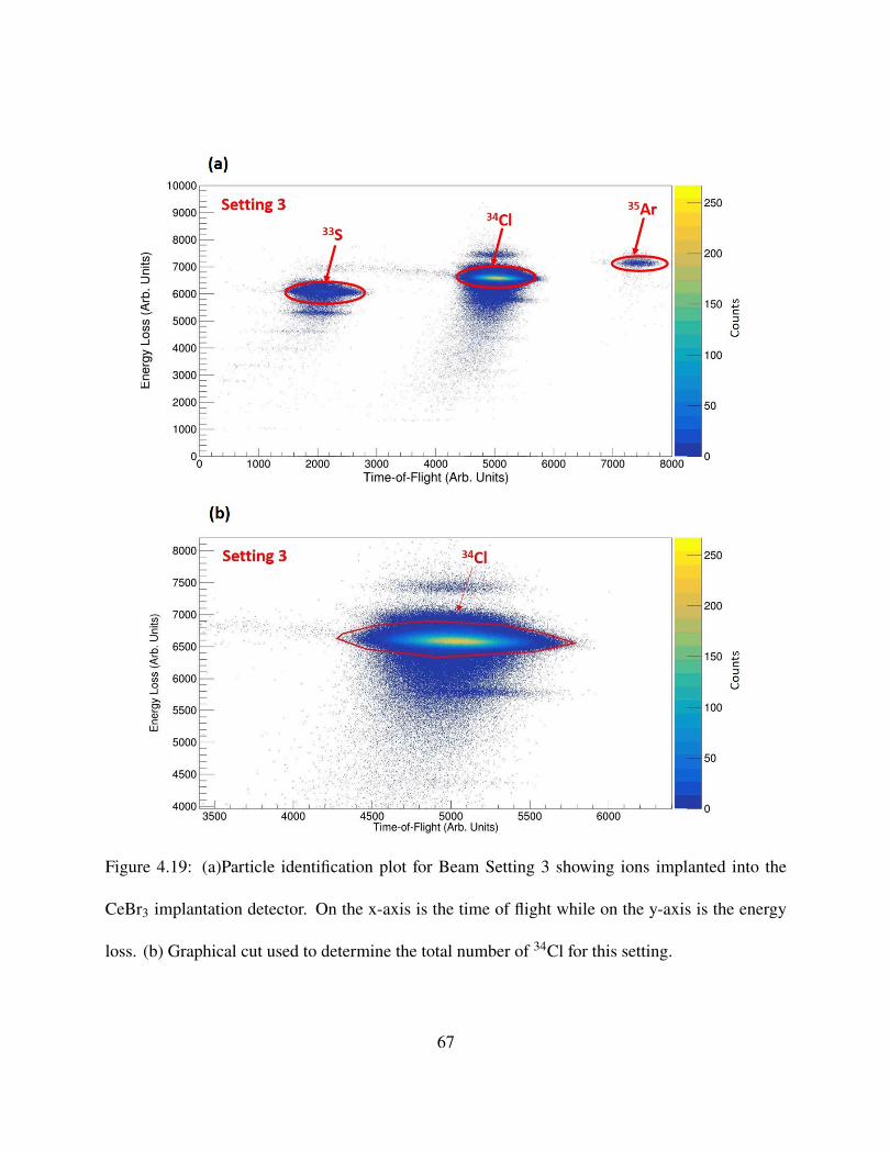
Figure 4.19: (a)Particle identification plot for Beam Setting 3 showing ions implanted into the
CeBr3 implantation detector. On the x-axis is the time of flight while on the y-axis is the energy
loss. (b) Graphical cut used to determine the total number of 34Cl for this setting.
67
Figure 4.20: (a)Particle identification plot for Beam Setting 4 showing ions implanted into the
CeBr3 implantation detector. On the x-axis is the time of flight while on the y-axis is the energy
loss. (b) Graphical cut used to determine the total number of 34Cl for this setting.
68

Figure 4.21: (a)Particle identification plot for Beam Setting 5 showing ions implanted into the
CeBr3 implantation detector. On the x-axis is the time of flight while on the y-axis is the energy
loss. (b) Graphical cut used to determine the total number of 34Cl for this setting.
69

Figure 4.22: (a)Particle identification plot for Beam Setting 6 showing ions implanted into the
CeBr3 implantation detector. On the x-axis is the time of flight while on the y-axis is the energy
loss. (b) Graphical cut used to determine the total number of 34Cl for this setting.
70

Beam Setting 2 and 3 PID plots (Fig. 4.18 and Fig. 4.19 respectively) display 33S and 34Cl
ion implantation. Beam Setting 3 plot additionally shows 35Ar was implanted into the CeBr3
implantation detector. The 35Ar could not be determined from a V-delayed W-ray spectrum because
98.23% of the time it decays from its ground state, Jc = 0+, to the ground state of 35Cl, without
emission of a W ray. Effort was made to find 35Ar in the correlated W-ray spectra since it has an
half-life of 1.7756(10) s, but the next highest order from intensity in 35Ar was too small (�abs =
0.249%) to be observed in the V-delayed W-ray spectrum. Beam Setting 4 indicates 33S, 34Cl and
35Ar. Lastly, Beam Setting 5 and 6 all show 32P, 33S and 34Cl was implanted into the detector.
4.3.4 Graphical cuts on the PID spectrum
To determine the total number of 34Cl ions implanted in the setup, a conservative approach was
taken by applying a large graphical cut as shown in Fig. 4.17 - Fig. 4.22. These large graphical
cuts was used as a compromise to maximize the number of 34Cl ions that were included in the
final result. The number of implanted 34Cl ion was then determined by taking the integrals of the
large graphical cuts. The uncertainties was estimated from the square root of the integral of the
graphical cut. There is an ongoing analysis to quantify the consistency of the graphical cuts used
in Fig. 4.17 - Fig. 4.22.
In conclusion, the number of 34Cl ions implanted into the CeBr3 detector during experi-
ment 16032A for each beam setting is shown in Table 4.8.
4.3.4.1 Determining transmission efficiency to the CeBr3 implantation detector.
The PID plots shown in Fig. 4.17 - Fig. 4.22 display ions which were detected by either the
first PIN detector or both the CeBr3 and the first PIN detector. This means that not all ions that
71

Table 4.8: Number of 34Cl isotope implanted into CeBr3 for each beam setting.
Beam Setting Number of Implanted 34Cl ions
1 1.7709(13) × 106
2 2.2355(15) × 106
3 1.7449(13) × 106
4 2.6679(16) × 106
5 1.7377(13) × 106
6 2.3482(15) × 106
were detected by the PIN detector will finally be implanted into the CeBr3. Only ions that implant
in our CeBr3 implantation detector could have W rays emitted from their decay observed in the
SeGA spectra. The transmission efficiency is then required to determine the overall probability that
ions passing through the PIN detectors subsequently implant into the CeBr3 implantation detector.
Transmission efficiency of the CeBr3 is the probability that ions detected in the PIN detector are
also implanted into the CeBr3 detector.
To determine the transmission efficiency for Beam Setting 1, the total counts of the PSPMT
dynode energy (indicating a signal in the CeBr3 implantation detector) was determined in coinci-
dence with a signal in the PIN detector and a PIN energy condition that excludes the possibility of
light ions that are unlikely to implant (see Fig. 4.23(a) and Table 4.9). Then, the number of counts
in the first PIN energy spectrum with the same energy condition so as to exclude the possibility
of light ions was also determined (see Fig. 4.23(b) and Table 4.9). Therefore, the transmission
efficiency to the CeBr3 implantation detector was determined by dividing the total counts of the
72

PSPMT dynode energy by the integrated PIN energy spectrum counts. Table 4.9 shows the trans-
mission efficiency of each beam setting. As expected, the transmission is very high (∼ 100%)
because the PIN detector is located very close to the CeBr3 implantation detector (approximately
1 meter upstream).
Table 4.9: Transmission efficiency from the first PIN detector to the CeBr3 implantation detector
for each beam setting.
Beam Setting CeBr3 counts PIN counts Transmission efficiency (%)
1 3.1490 × 10⁶ 3.1540 × 10⁶ 99.84
2 2.6790 × 10⁶ 2.6840 × 10⁶ 99.81
3 2.0400 × 10⁶ 2.0440 × 10⁶ 99.80
4 4.9160 × 10⁶ 4.9250 × 10⁶ 99.82
5 3.3210 × 10⁶ 3.3280 × 10⁶ 99.79
6 4.0380 × 10⁶ 4.0460 × 10⁶ 99.80
73

Figure 4.23: (a)CeBr3 implantation spectrum showing the PSPMT dynode energy. (b) PIN spec-
trum showing the energy loss in the PIN detector. The transmission efficiency to the implantation
detector will be the ratio of number at the top right corner in (a) to the number at the top right
corner in (b).
74

4.4 Isomeric ratio of 34Cl
From Table 4.7, Table 4.8 and Table 4.9, the isomeric state content ratio of 34Cl for Beam
Setting 1 is calculated as follow:
Number of ions of 34mCl implantedNumber of overall ions in the 34Cl beam
÷ Transmission efficiency
=5.04(24) × 105
1.7709(13) × 106 ÷ 0.9984 = 28.5(14)%(4.12)
By following similar pattern, Table 4.10 represents the final result for the isomeric state content ratio
of each Beam Setting for 34Cl. Since the number of 34mCl is divided by the number of implanted
34Cl ions, any fluctuations in beam intensity from the cyclotrons are normalized between the
different beam settings.
Table 4.10: Isomeric state content ratio of each beam setting in 34Cl.
Beam setting Isomeric content ratio of 34Cl beam
1 28.5(14)%
2 35.2(19)%
3 54.3(34)%
4 52.6(18)%
5 28.4(15)%
6 35.2(13)%
75

CHAPTER V
CONCLUSION
One of the main motivation for this experiment was to determine the Beam Setting to maximize
production of 34mCl. By maximizing the production of 34mCl, the highest abundant isomeric ratio
will be used to study the single neutron occupancies in high Mirror Energy Difference for 35Cl.
The importance of this measurement helps with the testing of single-particle aspects of the MED
states by extracting single neutron overlaps. Sec. 1.5 gives a detailed description for the motivation
of this experiment.
From the final result of the isomeric ratio of 34Cl for the six Beam Settings shown in Table 4.10,
Beam Setting 3 and Beam Setting 4 produces the highest isomer ratio of 54.3(34)% and 52.6(18)%
respectively. These settings has been recommended for use at the NSCL to study the single neutron
occupancy in 35Cl.
The result presented in this work does not include an analysis using the Batemann equation.
The time binning of the spectra for Bateman equation analysis has been developed. Ongoing
analysis is being done to fit the Bateman equation, which requires proper determination of both
the production and decay rates. Low statistics has made the analysis challenging thus far and we
currently lack full beam intensity information to perform the analysis accurately. We hope to have
the information soon.
76

Another future project focuses on building a better consistency for normalizing the graphical
cuts used to determine the final purities (Fig. 4.17 - Fig. 4.22). While conservative cuts were utilized
within uncertainty between one another, the differences in overall ToF between each A1900 setting
means a more exact normalization should be utilized. We will be working with the A1900 group
at the NSCL to finalize this aspect of the analysis.
77

REFERENCES
[1] J. I. Prisciandaro, Beta Decay Studies of 69Ni and 58V: Development of subshell gapswithin the N= 28-50 shell. PhD thesis, PhD thesis, Michigan State University, 2001.https://publications.nscl.msu.edu/thesis/Prisciandaro_2001_131.pdf.
[2] E. Rutherford, “LXXIX. The scattering of U and V particles by matter andthe structure of the atom,” The London, Edinburgh, and Dublin Philosophi-cal Magazine and Journal of Science, vol. 21, no. 125, pp. 669–688, 1911.http://mrmackenzie.co.uk/podpress_trac/feed/3110/0/Rutherford-paper.pdf.
[3] H. Gegier and E. Marsden, “On a diffuse reflection of the U-particles,” Pro-ceedings of the Royal Society of London. Series A, Containing Papers of aMathematical and Physical Character, vol. 82, no. 557, pp. 495–500, 1909.http://web.ihep.su/dbserv/compas/src/geiger09/eng.pdf.
[4] A. S. Panchbhai et al., “Wilhelm Conrad Röntgen and the discovery of X-rays:Revisited after centennial,” Journal of Indian academy of oral medicine and ra-diology, vol. 27, no. 1, p. 90, 2015. http://www.jiaomr.in/article.asp?issn=0972-1363;year=2015;volume=27;issue=1;spage=90;epage=95;aulast=Panchbhai.
[5] P.Gasparini, “History of radioactivity,” inUraniumgeochemistry, mineralogy, geology, explo-ration and resources, pp. 1–3, Springer, 1984. https://link.springer.com/chapter/10.1007/978-94-009-6060-2_1.
[6] N. Fröman, “Marie and Pierre Curie and the discovery of polonium and ra-dium,” Palestra na royal swedish academy of sciences, em Estocolmo, Sué-cia, 1996. https://www.nobelprize.org/prizes/uncategorized/marie-and-pierre-curie-and-the-discovery-of-polonium-and-radium-2/?print=1&guid=on.
[7] R. H. Paul Peter Urone, College physics. Opentextbc, 2012.https://opentextbc.ca/universityphysicsv3openstax/chapter/nuclear-binding-energy.
[8] H. L. Crawford, Evolution of nuclear shell structure: V-decay and isomeric prop-erties of nuclei in and near the fp shell. Michigan State University, 2010.https://groups.nscl.msu.edu/nscl_library/Thesis/Crawford,%20Heather.pdf.
[9] S. R. Stroberg, Single-particle structure of neutron-rich silicon isotopes and thebreakdown of the N= 28 shell closure. Michigan State University, 2014.https://pdfs.semanticscholar.org/2d5f/8567374a73b8842cbd809180cacbf6e41bf3.pdf.
78

[10] O. Haxel, J. H. D. Jensen, and H. E. Suess, “On the "magic num-bers"in nuclear structure,” Physical Review, vol. 75, no. 11, p. 1766, 1949.https://link.aps.org/pdf/10.1103/PhysRev.75.1766.2.
[11] M. G. Mayer, “On closed shells in nuclei. II,” Physical Review, vol. 75, no. 12, p. 1969, 1949.https://link.aps.org/pdf/10.1103/PhysRev.75.1969.
[12] A. Bohr and B. Mottelson, “Nuclear Structure. vol. 2. Nuclear Deformations,” 1975.
[13] G. K.K, Studies of shape changes of deformed nuclei and its effects oncluster emission. Department of physics, University of Calicut, 2012.https://shodhganga.inflibnet.ac.in/handle/10603/88449.
[14] M. R. Mumpower, T. Kawano, J. L. Ullmann, M. Krtička, and T. M. Sprouse, “Estimationof M 1 scissors mode strength for deformed nuclei in the medium-to heavy-mass region bystatistical Hauser-Feshbach model calculations,” Physical Review C, vol. 96, no. 2, p. 024612,2017. https://journals.aps.org/prc/abstract/10.1103/PhysRevC.96.024612.
[15] L. Bildsten, “Thermonuclear burning on rapidly accreting neutron stars,” inNATO Advanced Science Institutes (ASI) Series C, vol. 515, p. 419, 1998.https://ui.adsabs.harvard.edu/abs/1998ASIC..515..419B/abstract.
[16] C. Iliadis, A. Champagne, J. José, S. Starrfield, and P. Tupper, “The effectsof thermonuclear reaction-rate variations on nova nucleosynthesis: A sensitivitystudy,” The astrophysical Journal supplement series, vol. 142, no. 1, p. 105, 2002.https://iopscience.iop.org/article/10.1086/341400/meta.
[17] P. Banerjee, G. W. Misch, S. K. Ghorui, and Y. Sun, “Effective stellar V-decay rates of nucleiwith long-lived isomers: Al 26 and Cl 34,” Physical Review C, vol. 97, no. 6, p. 065807,2018. https://journals.aps.org/prc/abstract/10.1103/PhysRevC.97.065807.
[18] OpenStax, College Physics. Open Stax, 2012.
[19] G. T. S. Walter Loveland, David J. Morissey, Modern nuclear chem-istry. John Wiley and Sons, Inc., Hoboken, New Jersey, 2006.https://www.academia.edu/32900226/Modern_Nuclear_Chemistry_2nd_ed_-_Walter_D._Loveland_et_al._Wiley_2017_.
[20] G. Gilmore, Practical gamma-ray spectroscopy. John Wiley & Sons, 2011.https://www.tandfonline.com/doi/pdf/10.3109/00016925909173730.
[21] L. G. S. D. G. Sarantites, Introduction to the atomic nucleus. Washington, St Louis, 2012.http://chemistry.wustl.edu/ dgs/chem436/Lectures/Chem-436-Lecture_notes.pdf.
[22] hyperphysics, hyperphysic. Scilinks, 2001. http://hyperphysics.phy-astr.gsu.edu/hbase/quantum/fermi2.html#c1.
79
[23] W. Meyerhof, Elements of nuclear physics. McGraw-Hill, New York, 1967.https://ocw.mit.edu/courses/nuclear-engineering/22-101-applied-nuclear-physics-fall-2006/lecture-notes/lec22.pdf.
[24] D. J. Morrissey, G. T. Seaborg, and W. D. Loveland,Modern Nuclear Chemistry. John Wiley& Sons, 2006.
[25] L. van Dommelen, Quantum mechanics for engineers. Dommelen, 2004.http://www.eng.fsu.edu/ dommelen/quantum/style_a/index.html.
[26] G. Friedlander, J. W. Kennedy, E. S. Macias, and J. M. Miller, Nuclear and radiochemistry.John Wiley & Sons, 1981.
[27] K. S. Krane, D. Halliday, et al., Introductory nuclear physics. John Wiley & Sons, Inc., NewYork, 1987.
[28] G. Nelson and D. Reilly, “Gamma-ray interactions with matter,” Passive nondestructiveanalysis of nuclear materials, pp. 27–42, 1991. http://www.sciencemadness.org/lanl1_a/lib-www/la-pubs/00326397.pdf.
[29] S. N. Liddick, Beta-decay Studies of Neutron-rich Nuclides and the Possibility of an N: 34Subshell Closure. PhD thesis, Michigan State University. Department of Chemistry, 2004.http://publications.nscl.msu.edu/thesis/Liddick_2004_195.pdf.
[30] J. Cetnar, “General solution of Bateman equations for nuclear trans-mutations,” Annals of Nuclear Energy, vol. 33, no. 7, pp. 640–645,2006. https://www.sciencedirect.com/science/article/pii/S0306454906000284?c-asa_token=F_7tcitHUZkAAAAA:KouI8XR0e76YKqcUYnYA6XM7zNRXIn6L96bm-sxcNqstx6vXbz0qFNqxmRgUaN8WAAuxzGReyt_lu.
[31] A. Gade and B. Sherrill, “NSCL and FRIB at Michigan State University: Nuclearscience at the limits of stability,” Physica Scripta, vol. 91, no. 5, p. 053003, 2016.https://iopscience.iop.org/article/10.1088/0031-8949/91/5/053003/pdf.
[32] C. J. Prokop, Shape coexistence in the neutron-rich nickelisotopes near N= 40. Michigan State University, 2016.https://pdfs.semanticscholar.org/a66f/4c1bd570c96af242332694eec3f79842e477.pdf.
[33] D.Morrissey, “The coupled cyclotron project at theNSCL,”NuclearPhysics A, vol. 616, no. 1-2, pp. 45–55, 1997. https://www.sciencedirect.com/science/article/pii/S0375947497000730.
[34] C. T. Ramsell, Experimental study of an ion cyclotron resonance accelerator. PhDthesis, Michigan State University. Department of Physics and Astronomy, 2000.https://ieeexplore.ieee.org/stamp/stamp.jsp?arnumber=792423.
80

[35] J. Bin, Z. Zhen-Lu, Z. Tian-Jue, X. Jian-Sheng, W. Xiu-Long, Y. Zhi-Guo, H. Shi-Gang, andX. Le, “Theoretical and Practical study onRFModel Cavity of 100mevH-Cyclotron,”ChinesePhysics C, vol. 32, no. S1, pp. 160–162, 2008. http://cpc.ihep.ac.cn/article/id/97e18b16-cd0d-42f0-be93-c4c9e9ac5a94.
[36] P. K. Sigg, “RF for cyclotrons,” 2006. https://cds.cern.ch/record/1005053/files/p231.pdf.
[37] S. M. Lund, “Accelerator physics.” Exotic beam summer school, Michigan State university,National Super Conducting Laboratory (NSCL), 2016.
[38] B.-M. Sherrill, “Scientific opportunities with the NSCL coupled cyclotron facil-ity,” Progress of Theoretical Physics Supplement, vol. 146, pp. 60–69, 2002.https://academic.oup.com/ptps/article/doi/10.1143/PTPS.146.60/1864439.
[39] A. W. Chao, K. H. Mess, et al., Handbook of accel-erator physics and engineering. World scientific, 2013.https://books.google.com/books?hl=en&lr=&id=W4C6CgAAQBAJ&oi=fnd&pg=PR-5&dq=Handbook+of+accelerator+physics+and+engineering&ots=696Y_H244C&sig-=woigLpWaE_lZKqz35_wyJRnqFRA.
[40] M. Mocko, Rare isotope production. PhD thesis, MichiganState University. Department of Physics and Astronomy, 2006.https://groups.nscl.msu.edu/nscl_library/Thesis/Mocko,%20Michal.pdf.
[41] P. van Duppen, “Noyaux exotiques: production propriétés et spécificités,” 1997.https://cel.archives-ouvertes.fr/cel-00652717/document.
[42] S. Paschalis, “Studies of exotic nuclei: state-of-the-art experimental tools and techniques,”in Journal of Physics: Conference Series, vol. 599, p. 012032, IOP Publishing, 2015.https://iopscience.iop.org/article/10.1088/1742-6596/599/1/012032/pdf.
[43] D. J. Morrissey and B. M. Sherrill, “Radioactive nuclear beam facilities based on projec-tile fragmentation,” Philosophical Transactions of the Royal Society of London. Series A:Mathematical, Physical and Engineering Sciences, vol. 356, no. 1744, pp. 1985–2006, 1998.https://royalsocietypublishing.org/doi/pdf/10.1098/rsta.1998.0260.
[44] T. Otsuka, “Exotic nuclei and nuclear forces,” Physica Scripta, vol. 2013, no. T152, p. 014007,2013. https://iopscience.iop.org/article/10.1088/0031-8949/2013/T152/014007/pdf.
[45] D. . J. Morrissey, B. Sherrill, M. Steiner, A. Stolz, and I. Wiedenhoever, “Commissioningthe A1900 projectile fragment separator,” Nuclear Instruments and Methods in Physics Re-search Section B: Beam Interactions with Materials and Atoms, vol. 204, pp. 90–96, 2003.https://www.sciencedirect.com/science/article/pii/S0168583X02018955.
[46] K. M. McElroy, “Measurement of fragment transmission in the A1900 fragment separator,”https://pdfs.semanticscholar.org/54b9/37247076336583001e296f0e4f56f30bffe7.pdf.
81

[47] T. Baumann, “Minicourse on experimental techniques at the NSCL fragment separators,”2001. https://people.nscl.msu.edu/ baumann/frs_lecture.pdf.
[48] A. Stolz, T. Baumann, T. Ginter, D. Morrissey, M. Portillo, B. Sherrill, M. Steiner,and J. Stetson, “Production of rare isotope beams with the NSCL fragment sep-arator,” Nuclear Instruments and Methods in Physics Research Section B: BeamInteractions with Materials and Atoms, vol. 241, no. 1-4, pp. 858–861, 2005.https://www.sciencedirect.com/science/article/pii/S0168583X0501339X.
[49] B. S. Ninel Nica, “Electron capture decay of 34Cl,” 2012.https://www.nndc.bnl.gov/nudat2/decaysearchdirect.jsp?nuc=34CL&unc=nds.
[50] N. Nica and B. Singh, “Nuclear data sheets for A= 34,” Nu-clear data sheets, vol. 113, no. 6-7, pp. 1563–1733, 2012.https://www.sciencedirect.com/science/article/pii/S0090375212000488.
[51] K. Heyde and J. L. Wood, “Shape coexistence in atomic nuclei,” Reviews of Modern Physics,vol. 83, no. 4, p. 1467, 2011. https://link.aps.org/pdf/10.1103/RevModPhys.83.1467.
[52] O. Tarasov and D. Bazin, “LISE++: Exotic beam production with fragment sep-arators and their design,” Nuclear Instruments and Methods in Physics ResearchSection B: Beam Interactions with Materials and Atoms, vol. 376, pp. 185–187, 2016.https://www.sciencedirect.com/science/article/pii/S0168583X1600224X?casa_token=G-o0KWEVBJ6UAAAAA:tkupTPZ7L6fwcavNsxiXoDZlCJoaZwx4DEeSAPAfAN3MpG-WO4ja1Vz7hPaYnPaCQ3tVHWeUpqf1T.
[53] C. Meeks and P. Siegel, “Dead time correction via the time se-ries,” American Journal of Physics, vol. 76, no. 6, pp. 589–590, 2008.https://aapt.scitation.org/doi/pdf/10.1119/1.2870432.
[54] H. J. J. Cleaves, Branching Ratio. Springer Berlin Heidelberg, 2011.https://doi.org/10.1007/978-3-642-11274-4_206.
82