Studyof mass sensitive parametersfor AMIGA and AERA ...personalpages.to.infn.it/~bertaina/tesi-scaricate/... · Studyof mass sensitive parametersfor AMIGA and AERA cosmicraydetectors

Study of mass sensitive parameters for AMIGA and AERA cosmic ray detectors

Relatori: Prof. Bertaina Mario Edoardo

Dr. Haungs Andreas

Corelatore: Mr. Stuani Pereira Luiz Augusto

1Daniele Proverbio - a.a. 2015/16 - UNITO

A.A. 2015/2016Università degli Studi di Torino – Dipartimento di Fisica

Luglio 2016

Candidato: Proverbio Daniele

Where: Karlsruhe Institute of TechnologyErasmus Traineeship Project

Karlsruhe, Baden-Württemberg, Germany

KIT – Campus North


Who

The Institut für Kernphysik Group

Add photo


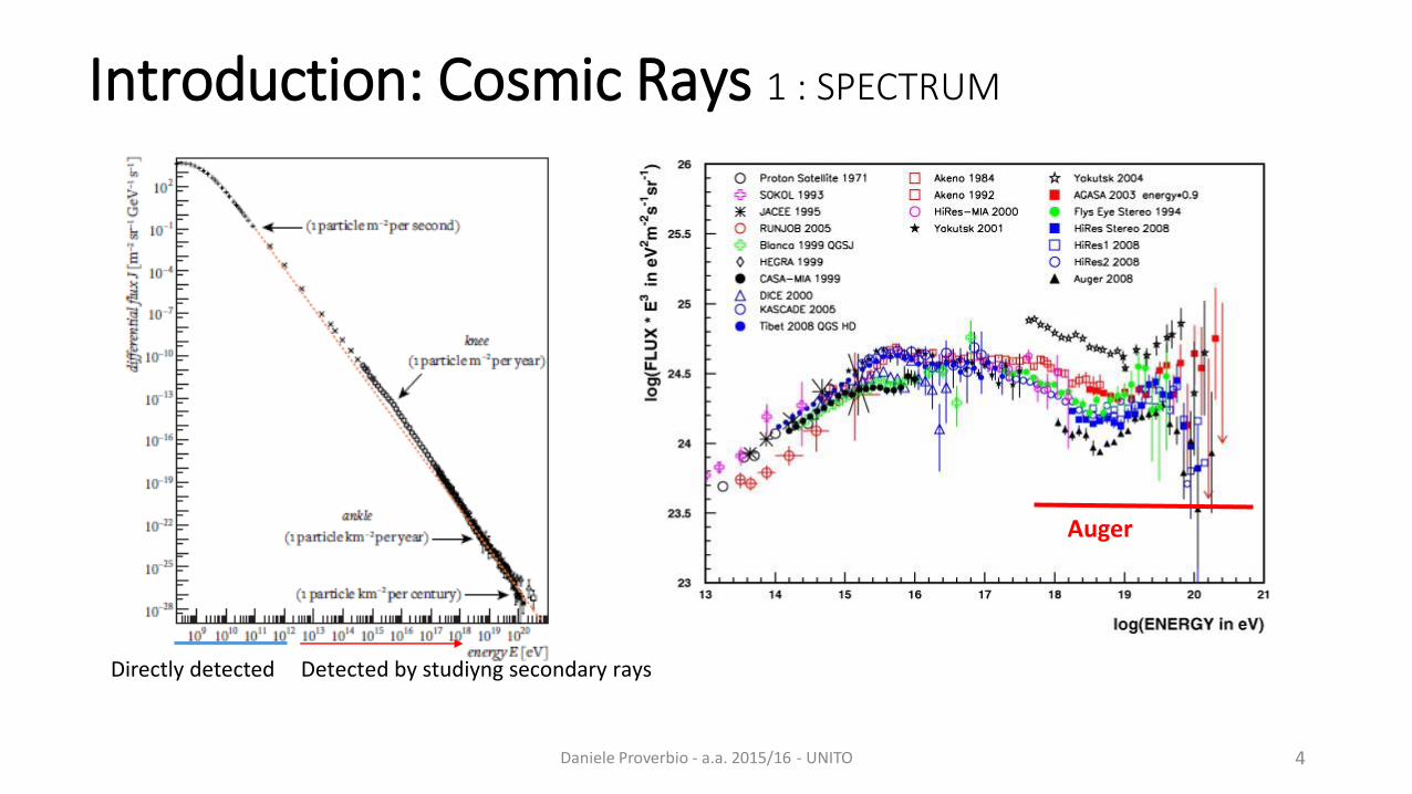
Introduction: Cosmic Rays 1 : SPECTRUM

4

Directly detected Detected by studiyng secondary rays

Auger

Daniele Proverbio - a.a. 2015/16 - UNITO

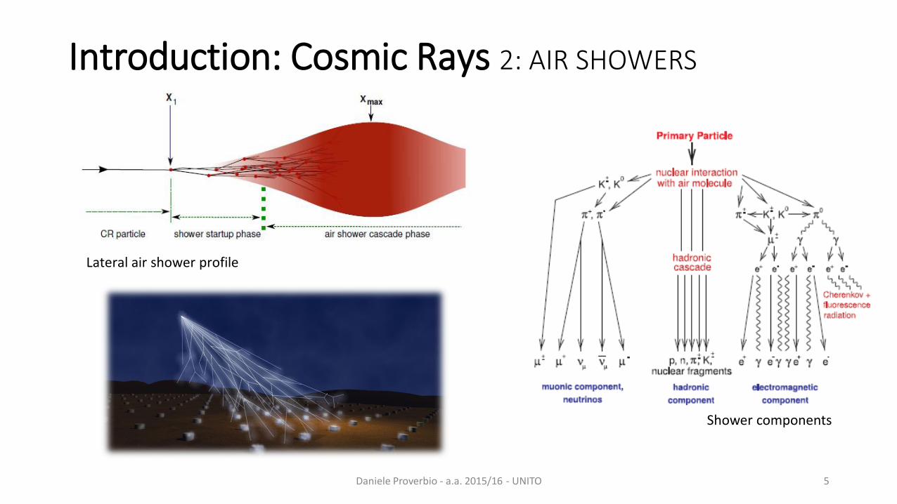
Introduction: Cosmic Rays 2: AIR SHOWERS

5

Lateral air shower profile

Shower components


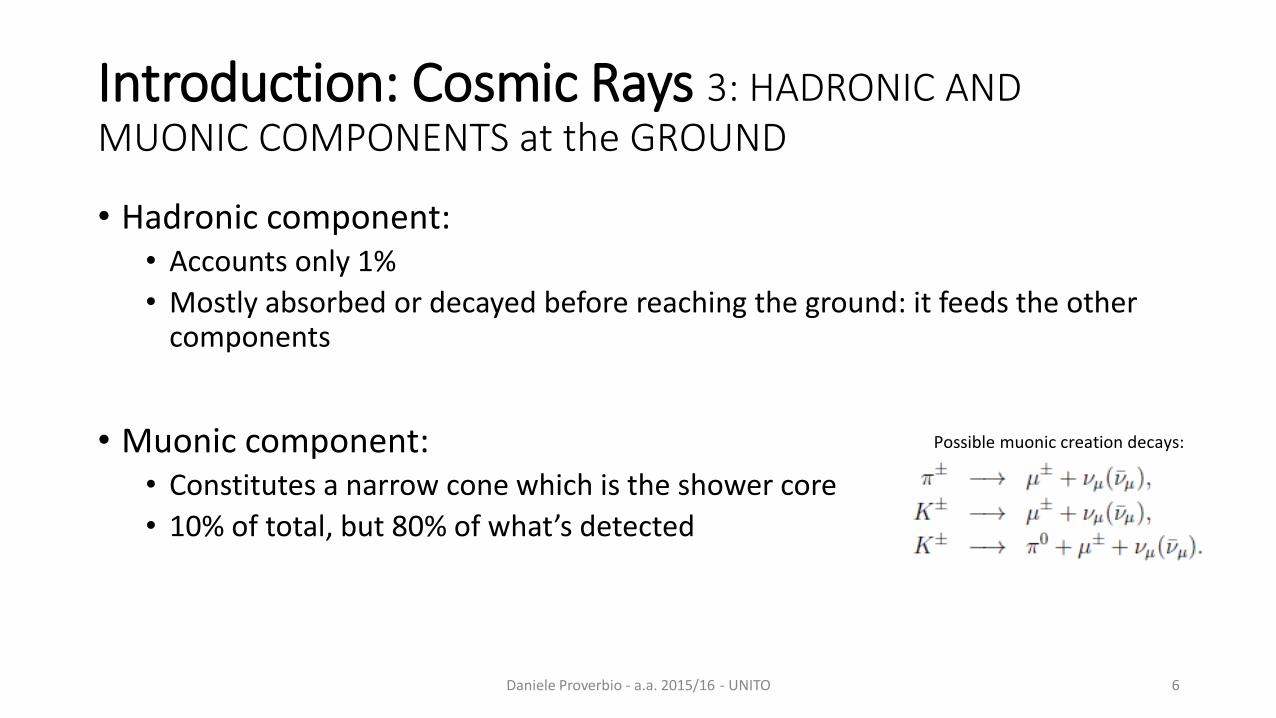
Introduction: Cosmic Rays 3: HADRONIC AND MUONIC COMPONENTS at the GROUND

• Hadronic component:• Accounts only 1%

• Mostly absorbed or decayed before reaching the ground: it feeds the othercomponents

• Muonic component:• Constitutes a narrow cone which is the shower core

• 10% of total, but 80% of what’s detected

6

Possible muonic creation decays:


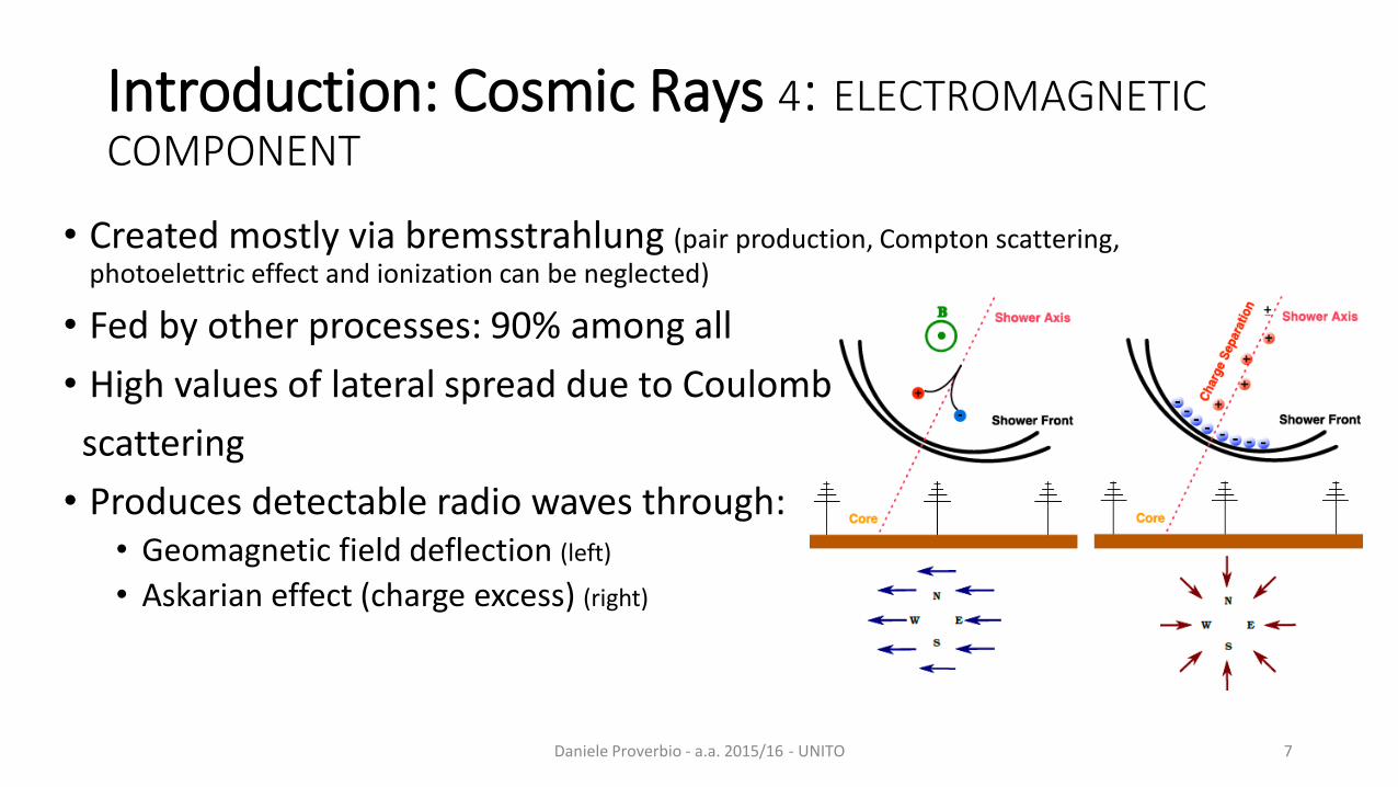
Introduction: Cosmic Rays 4: ELECTROMAGNETIC COMPONENT

• Created mostly via bremsstrahlung (pair production, Compton scattering, photoelettric effect and ionization can be neglected)

• Fed by other processes: 90% among all

• High values of lateral spread due to Coulomb

scattering

• Produces detectable radio waves through:• Geomagnetic field deflection (left)

• Askarian effect (charge excess) (right)


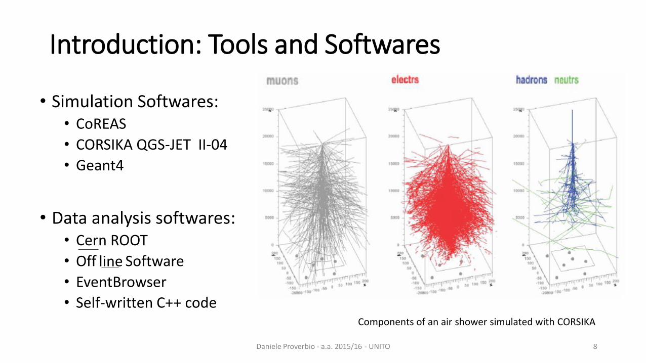
Introduction: Tools and Softwares

• Simulation Softwares:• CoREAS

• CORSIKA QGS-JET II-04

• Geant4

• Data analysis softwares:• Cern ROOT

• Off Software

• EventBrowser

• Self-written C++ code

8

line

Components of an air shower simulated with CORSIKA


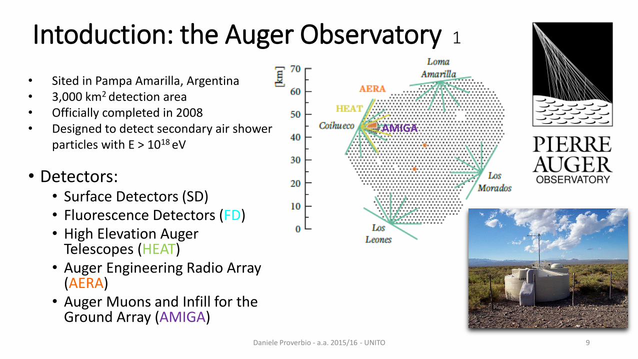
Intoduction: the Auger Observatory 1


• Sited in Pampa Amarilla, Argentina• 3,000 km2 detection area• Officially completed in 2008• Designed to detect secondary air shower

particles with E > 1018 eV

• Detectors:• Surface Detectors (SD) • Fluorescence Detectors (FD)• High Elevation Auger

Telescopes (HEAT)• Auger Engineering Radio Array

(AERA)• Auger Muons and Infill for the

Ground Array (AMIGA)

AMIGA

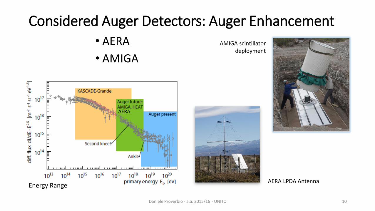
Considered Auger Detectors: Auger EnhancementAERA•

AMIGA•

Daniele Proverbio - a.a. 2015/16 - UNITO 10

AERA

Energy RangeAERA LPDA Antenna

AMIGA scintillatordeployment

GoalCombine AERA and AMIGA • measurements

Look for • correlations between Erad and Nμ

Combine • results with simulations

Study• mass estimator parameters

11

Exploit combined measurementsto figure out the mass composition of primary cosmic rays

using mass estimators

Here we start Daniele Proverbio - a.a. 2015/16 - UNITO

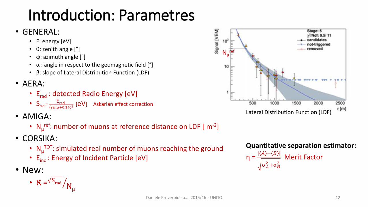
Introduction: ParametresGENERAL:•

E: • energy [eV]

• θ: zenith angle [°]

• φ: azimuth angle [°]

• α : angle in respect to the geomagnetic field [°]

• β: slope of Lateral Distribution Function (LDF)

AERA:•• Erad : detected Radio Energy [eV]

• Srad = Erad

𝑠𝑖𝑛α+0.14 2 [eV] Askarian effect correction

AMIGA:•• Nμ

ref: number of muons at reference distance on LDF [ m-2]

CORSIKA:•• Nμ

TOT: simulated real number of muons reaching the ground• Einc : Energy of Incident Particle [eV]

New:•

• ℵ = ൗSrad

Nμ

12

Offline LDF fit


Quantitative separation estimator:

η = |⟨𝐴⟩−⟨𝐵⟩|

σ𝐴2+σ𝐵

2Merit Factor

Lateral Distribution Function (LDF)

Nμref

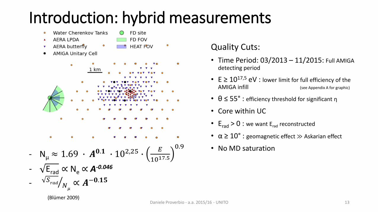
Introduction: hybrid measurements


- Nμ ≈ 1.69 ∙ 𝑨𝟎.𝟏 ∙ 102,25 ∙𝐸

1017.5

0.9

- Erad ∝ Ne ∝ A-0.046

- ൗ𝑆𝑟𝑎𝑑 𝑁𝜇∝ 𝑨−𝟎.𝟏𝟓

(Blümer 2009)

Quality Cuts:

• Time Period: 03/2013 – 11/2015: Full AMIGA detecting period

• E ≥ 1017,5 eV : lower limit for full efficiency of the AMIGA infill (see Appendix A for graphic)

• θ ≤ 55° : efficiency threshold for significant η

• Core within UC

• Erad > 0 : we want Erad reconstructed

• α ≥ 10° : geomagnetic effect ≫ Askarian effect

• No MD saturation

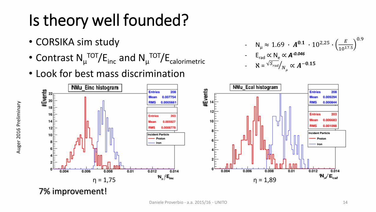
Is theory well founded?• CORSIKA sim study

• Contrast NμTOT/Einc and Nμ

TOT/Ecalorimetric

• Look for best mass discrimination


η = 1,75 η = 1,89

7% improvement!

- Nμ ≈ 1.69 ∙ 𝑨𝟎.𝟏 ∙ 102,25 ∙𝐸

1017.5

0.9

- Erad ∝ Ne ∝ A-0.046

- ℵ = ൗ𝑆𝑟𝑎𝑑 𝑁𝜇

∝ 𝑨−𝟎.𝟏𝟓

Au

ger

2016

Pre

limin

ary

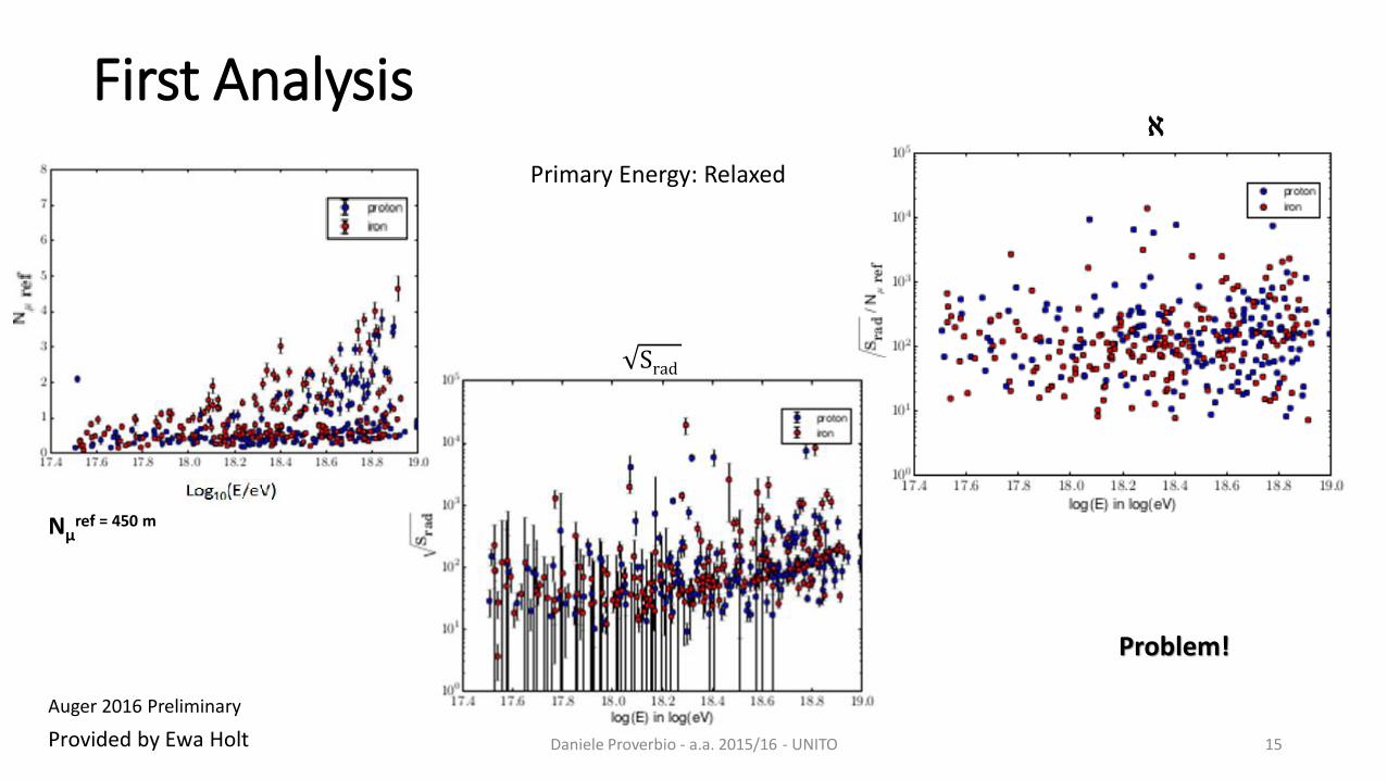
First Analysis


Primary Energy: Relaxed

Provided by Ewa Holt

Nμref = 450 m

Srad

ℵ

Problem!

Auger 2016 Preliminary

Work Plan

• DEBUGGING: look for the reason(s) why the masscomposition estimation is failing

• IMPROVING: overcome the problem and get the correctparameters

• ANALYSING: re-try the analysis with the correctedparameters and evaluate the massdiscrimination power

• GOING FURTHER


Looking for unexpected features: DEBUGGING

Mass • separation fails: causes?Different• methods or bias from CoRSIKA QSG-JET II-04 (Shower simulation) to Offline (Detectors’ reconstruction)?

Reference • distance fixed at r0 = 450 m: is it ok?

• Erad behavior?

Therefore• : Compare • simulations with reconstructions, applying quality cuts and contrasting main parameters (namely Nµ

ref vs NµTOT and Erad vs Einc)

Compare • r0 with literature.


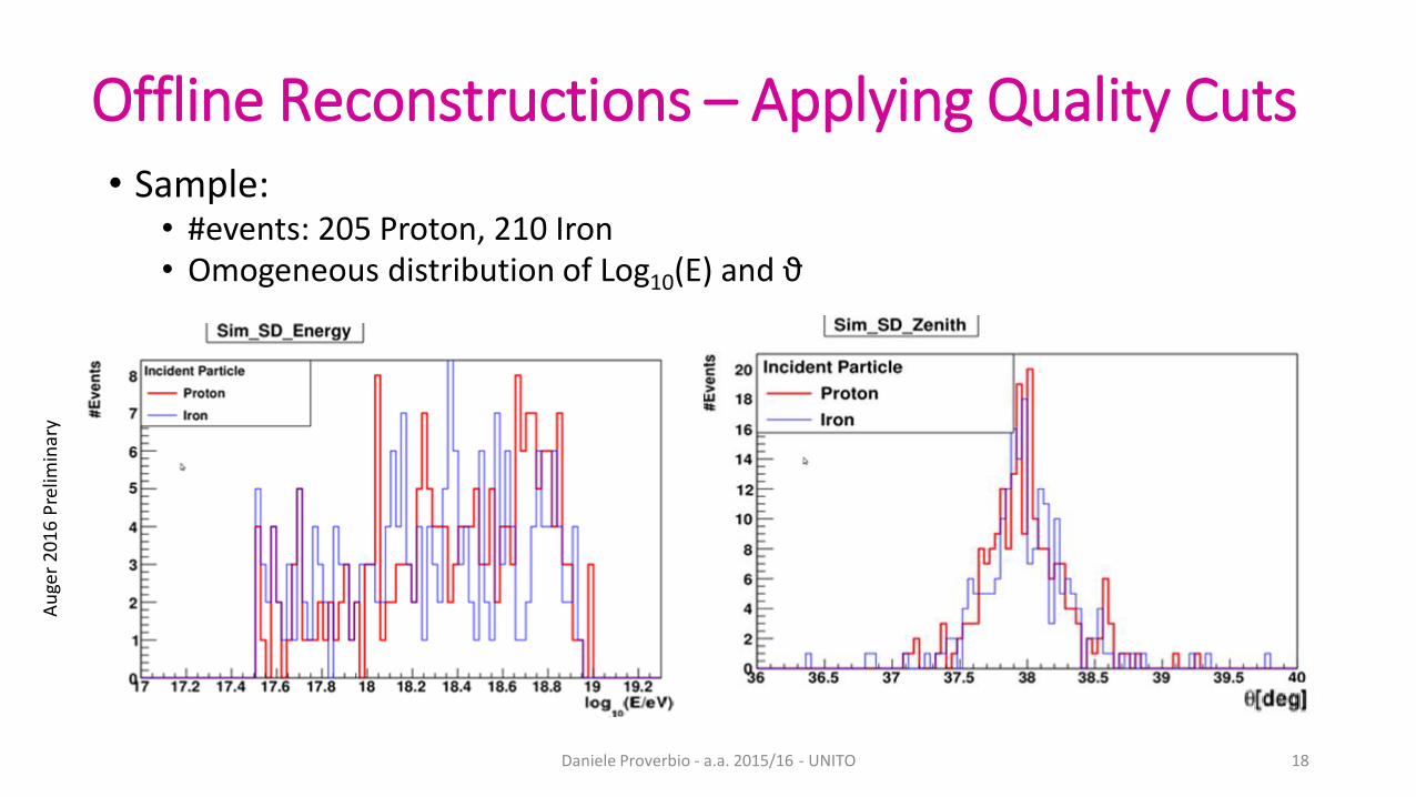
Offline Reconstructions – Applying Quality Cuts• Sample:

• #events: 205 Proton, 210 Iron• Omogeneous distribution of Log10(E) and ϑ


Au

ger

2016

Pre

limin

ary

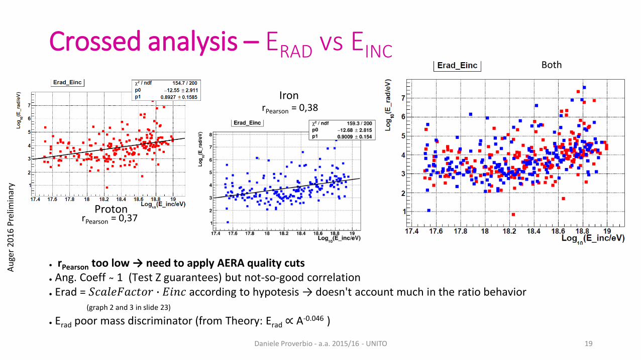
Crossed analysis – ERAD vs EINC


Proton

Iron

● rPearson too low → need to apply AERA quality cuts● Ang. Coeff ̴ 1 (Test Z guarantees) but not-so-good correlation● Erad = 𝑆𝑐𝑎𝑙𝑒𝐹𝑎𝑐𝑡𝑜𝑟 ∙ 𝐸𝑖𝑛𝑐 according to hypotesis → doesn't account much in the ratio behavior

(graph 2 and 3 in slide 23)

● Erad poor mass discriminator (from Theory: Erad ∝ A-0.046 )

Both

rPearson = 0,37

rPearson = 0,38

Au

ger

2016

Pre

limin

ary

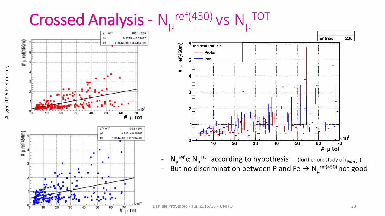
Crossed Analysis - Nµref(450) vs Nµ

TOT


- Nµref α Nµ

TOT according to hypothesis (further on: study of rPearson)

But no discrimination between P and Fe - → Nμref(450) not good

Au

ger

2016

Pre

limin

ary

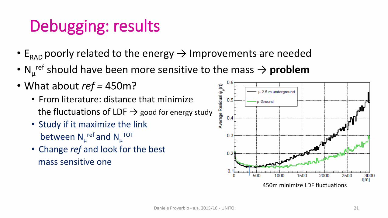
Debugging: results

• ERAD poorly related to the energy → Improvements are needed

• Nµref should have been more sensitive to the mass → problem

What• about ref = 450m?From • literature: distance that minimize

the fluctuations of LDF → good for energy study

Study• if it maximize the link

between Nµref and Nµ

TOT

Change • ref and look for the best

mass sensitive one


450m minimize LDF fluctuations

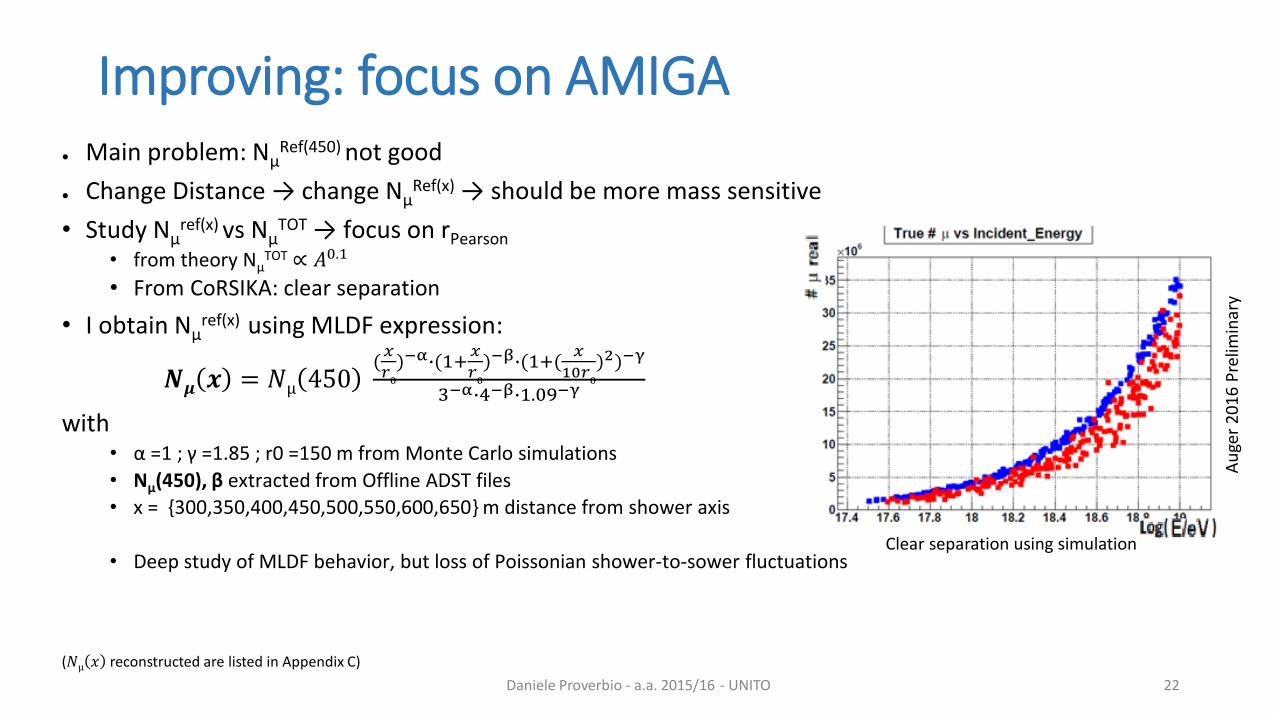
Improving: focus on AMIGAMain problem: N● μ

Ref(450) not good

Change Distance ● → change NμRef(x) → should be more mass sensitive

Study• Nµref(x) vs Nµ

TOT → focus on rPearsonfrom theory N• µ

TOT ∝ 𝐴0.1

From • CoRSIKA: clear separation

I • obtain Nµref(x) using MLDF expression:

𝑵𝝁 𝒙 = 𝑁μ 450(𝑥

𝑟0

)−α∙(1+𝑥

𝑟0

)−β∙(1+(𝑥

10𝑟0

)2)−γ

3−α∙4−β∙1.09−γ

withα =• 1 ; γ =1.85 ; r0 =150 m from Monte Carlo simulations

• Nμ(450), β extracted from Offline ADST files

x = {• 300,350,400,450,500,550,600,650} m distance from shower axis

Deep• study of MLDF behavior, but loss of Poissonian shower-to-sower fluctuations


(𝑁μ 𝑥 reconstructed are listed in Appendix C)

Clear separation using simulation

Au

ger

2016

Pre

limin

ary

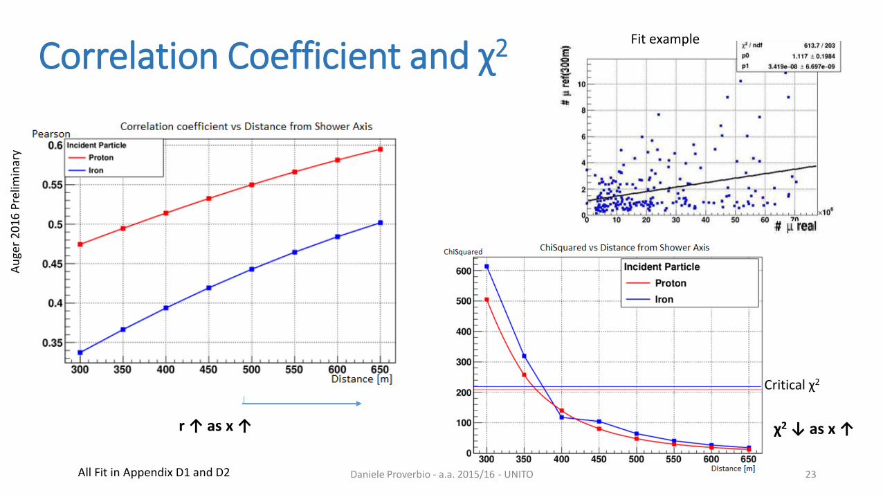
Correlation Coefficient and χ2


Critical χ2

r ↑ as x ↑ χ2 ↓ as x ↑

All Fit in Appendix D1 and D2

Fit example

Au

ger

2016

Pre

limin

ary

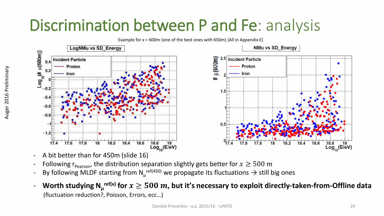
Discrimination between P and Fe: analysis


Example for x = 600m (one of the best ones with 650m) [All in Appendix E]

A bit - better than for 450m (slide 16)Following- rPearson, the distribution separation slightly gets better for 𝑥 ≥ 500 𝑚By - following MLDF starting from Nμ

ref(450) we propagate its fluctuations → still big ones

Worth - studying Nμref(x) for 𝒙 ≥ 𝟓𝟎𝟎𝒎, but it’s necessary to exploit directly-taken-from-Offline data

(fluctuation reduction?, Poisson, Errors, ecc…)

Au

ger

2016

Pre

limin

ary

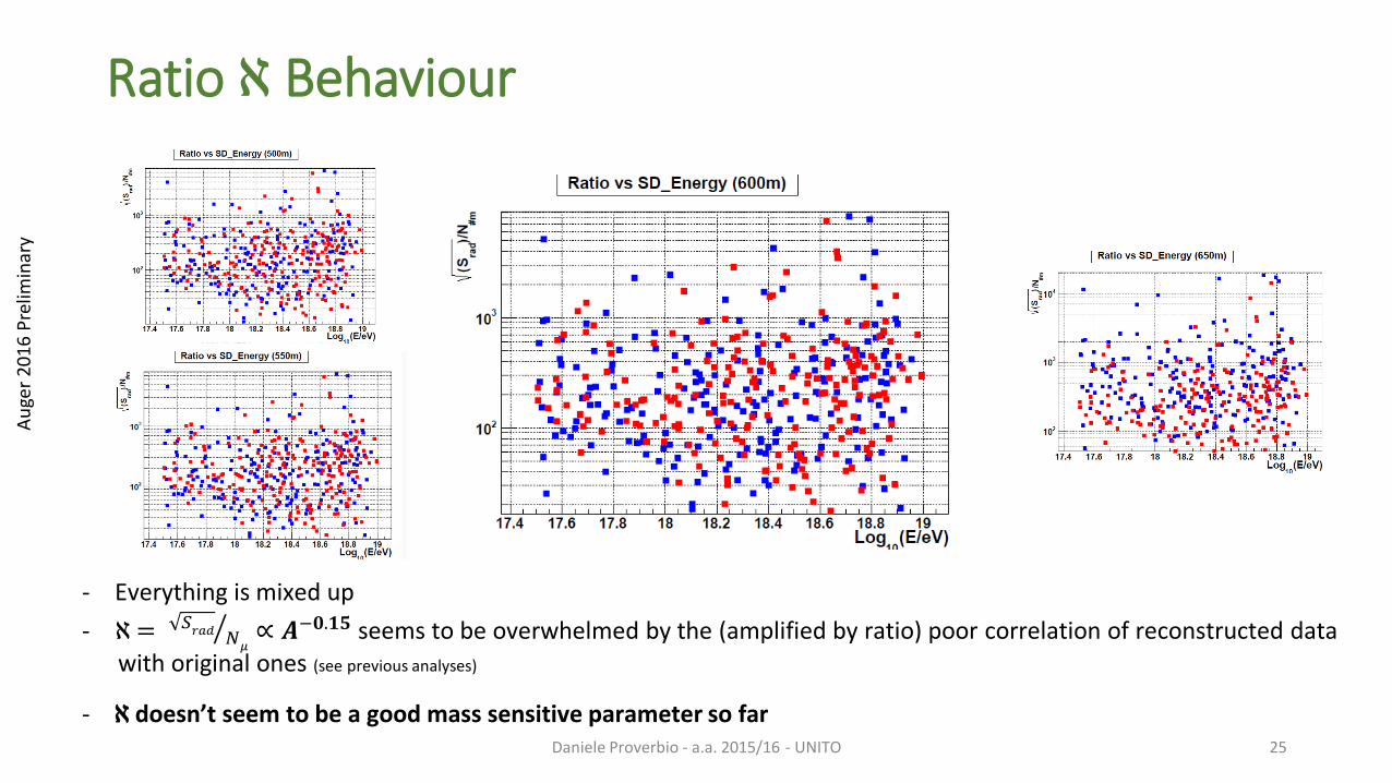
Ratio ℵ Behaviour


Everything - is mixed up

- ℵ = ൗ𝑆𝑟𝑎𝑑 𝑁𝜇∝ 𝑨−𝟎.𝟏𝟓 seems to be overwhelmed by the (amplified by ratio) poor correlation of reconstructed data

with original ones (see previous analyses)

- ℵ doesn’t seem to be a good mass sensitive parameter so far

Au

ger

2016

Pre

limin

ary

Conclusions: mass estimationNecessary• to change ref → Nμ

ref > 500m ;

As• seen from simulations, ℵ = ൗ𝑆𝑟𝑎𝑑 𝑁

𝜇is worth studying, but it must be

improved

Suggested• improvements:• Erad → AERA quality cuts, noise packages

• Nμref

Consider• data directly extracted from Offline

Change• ref and determine the most sensitive one crossing rPearson, χ2 results and real MLDFfluctuation and μ detection

Consider• other AMIGA parameters e.g. 300

+∞𝑀𝐿𝐷𝐹 𝑑𝑥

Other• strategies


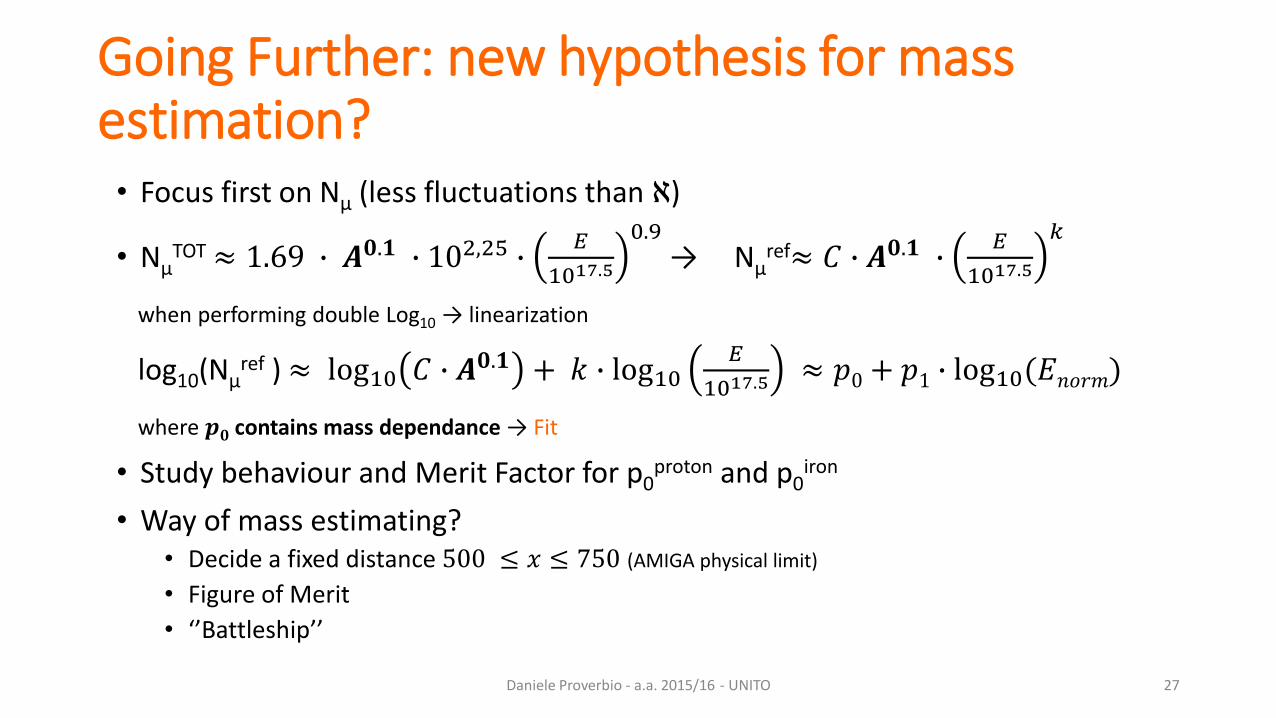
Going Further: new hypothesis for mass estimation?


• Focus first on Nμ (less fluctuations than ℵ)

• NμTOT ≈ 1.69 ∙ 𝑨𝟎.𝟏 ∙ 102,25 ∙

𝐸

1017.5

0.9→ Nμ

ref≈ 𝐶 ∙ 𝑨𝟎.𝟏 ∙𝐸

1017.5

𝑘

when performing double Log10 → linearization

log10(Nμref ) ≈ log10 𝐶 ∙ 𝑨𝟎.𝟏 + 𝑘 ∙ log10

𝐸

1017.5≈ 𝑝0+ 𝑝1 ∙ log10(𝐸𝑛𝑜𝑟𝑚)

where 𝒑𝟎 contains mass dependance → Fit

• Study behaviour and Merit Factor for p0proton and p0

iron

• Way of mass estimating?• Decide a fixed distance 500 ≤ 𝑥 ≤ 750 (AMIGA physical limit)

• Figure of Merit

• ‘’Battleship’’

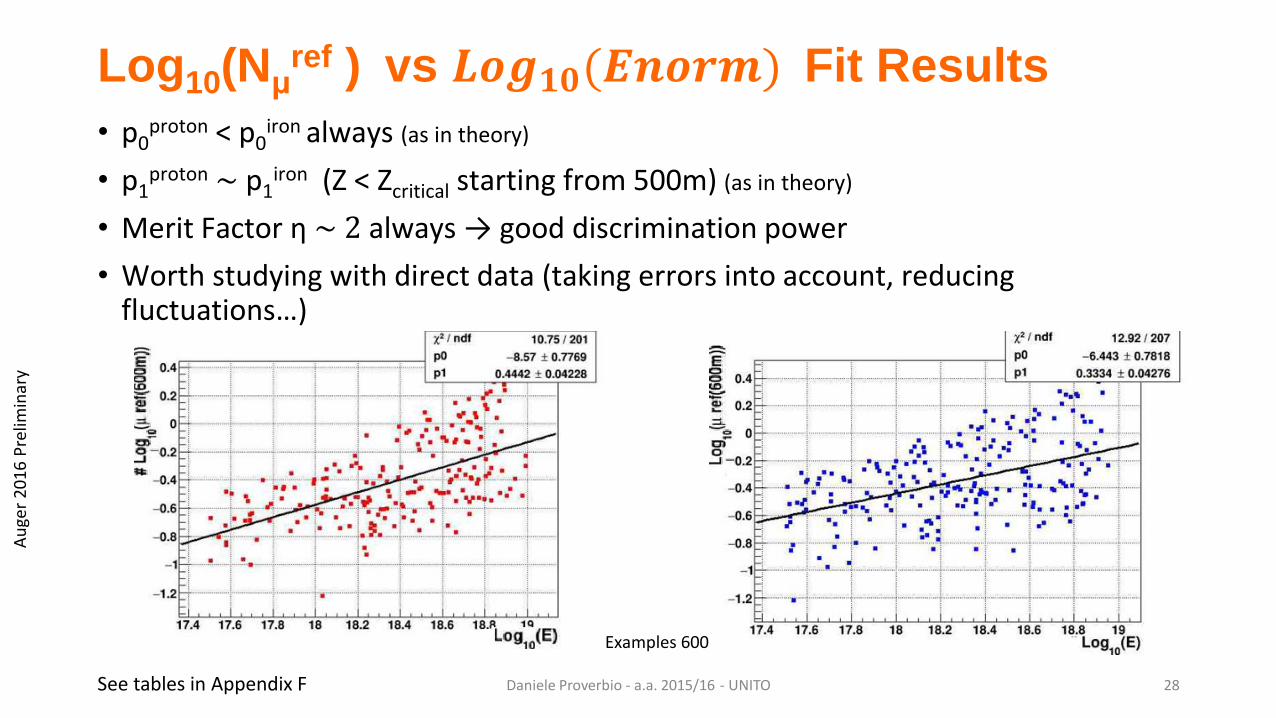
Log10(Nμref ) vs 𝑳𝒐𝒈𝟏𝟎(𝑬𝒏𝒐𝒓𝒎) Fit Results

• p0proton < p0

iron always (as in theory)

• p1proton ~ p1

iron (Z < Zcritical starting from 500m) (as in theory)

Merit• Factor η ~ 2 always → good discrimination power

Worth • studying with direct data (taking errors into account, reducingfluctuations…)


Fit Examples 600m

See tables in Appendix F

Au

ger

2016

Pre

limin

ary

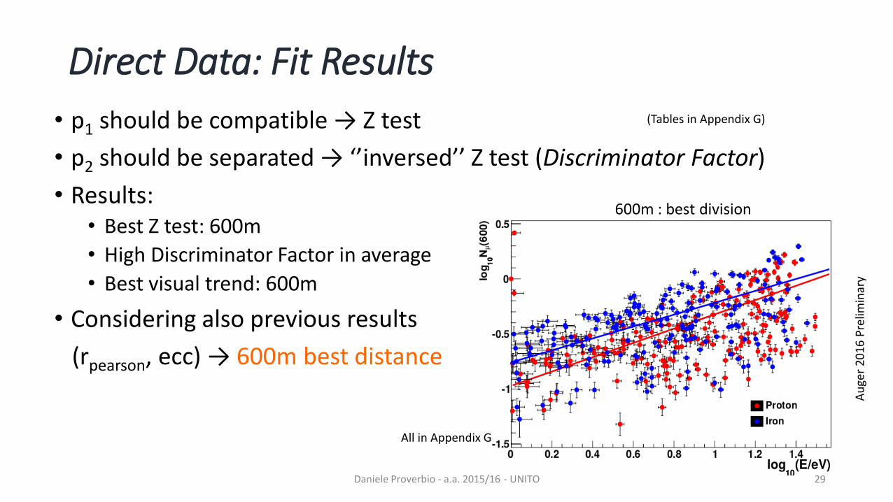
Direct Data: Fit Results

• p1 should be compatible → Z test

• p2 should be separated → ‘’inversed’’ Z test (Discriminator Factor)

• Results:• Best Z test: 600m

• High Discriminator Factor in average

• Best visual trend: 600m

• Considering also previous results

(rpearson, ecc) → 600m best distance


All in Appendix G

600m : best division

(Tables in Appendix G)

Au

ger

2016

Pre

limin

ary

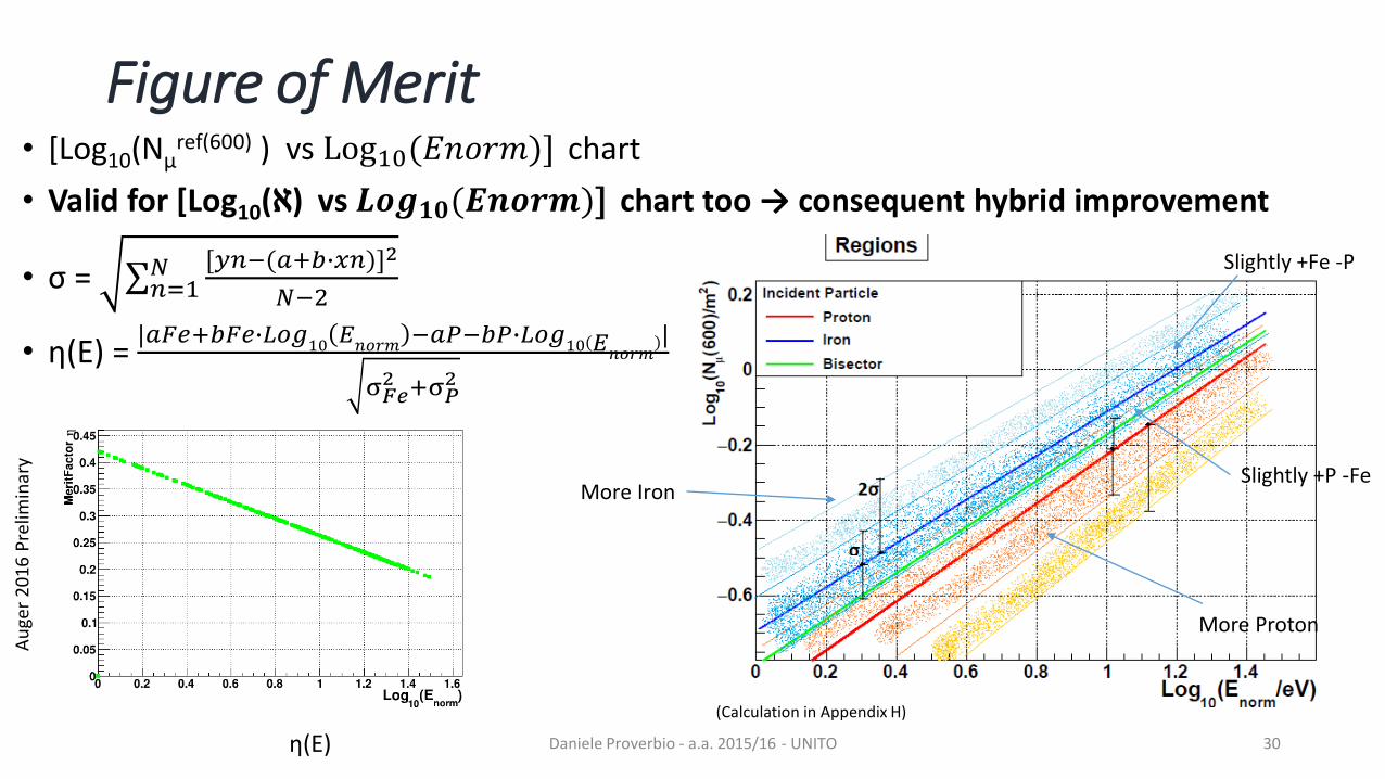
Figure of Merit• [Log10(Nμ

ref(600) ) vs Log10(𝐸𝑛𝑜𝑟𝑚)] chart

• Valid for [Log10(ℵ) vs 𝑳𝒐𝒈𝟏𝟎(𝑬𝒏𝒐𝒓𝒎)] chart too → consequent hybrid improvement

• σ = σ𝑛=1𝑁 [𝑦𝑛−(𝑎+𝑏∙𝑥𝑛)]2

𝑁−2

• η(E) = |𝑎𝐹𝑒+𝑏𝐹𝑒∙𝐿𝑜𝑔

10𝐸𝑛𝑜𝑟𝑚

−𝑎𝑃−𝑏𝑃∙𝐿𝑜𝑔10 𝐸𝑛𝑜𝑟𝑚

|

σ𝐹𝑒2 +σ𝑃

2


(Calculation in Appendix H)

Slightly +Fe -P

Slightly +P -FeMore Iron

More Proton

η(E)

Au

ger

2016

Pre

limin

ary

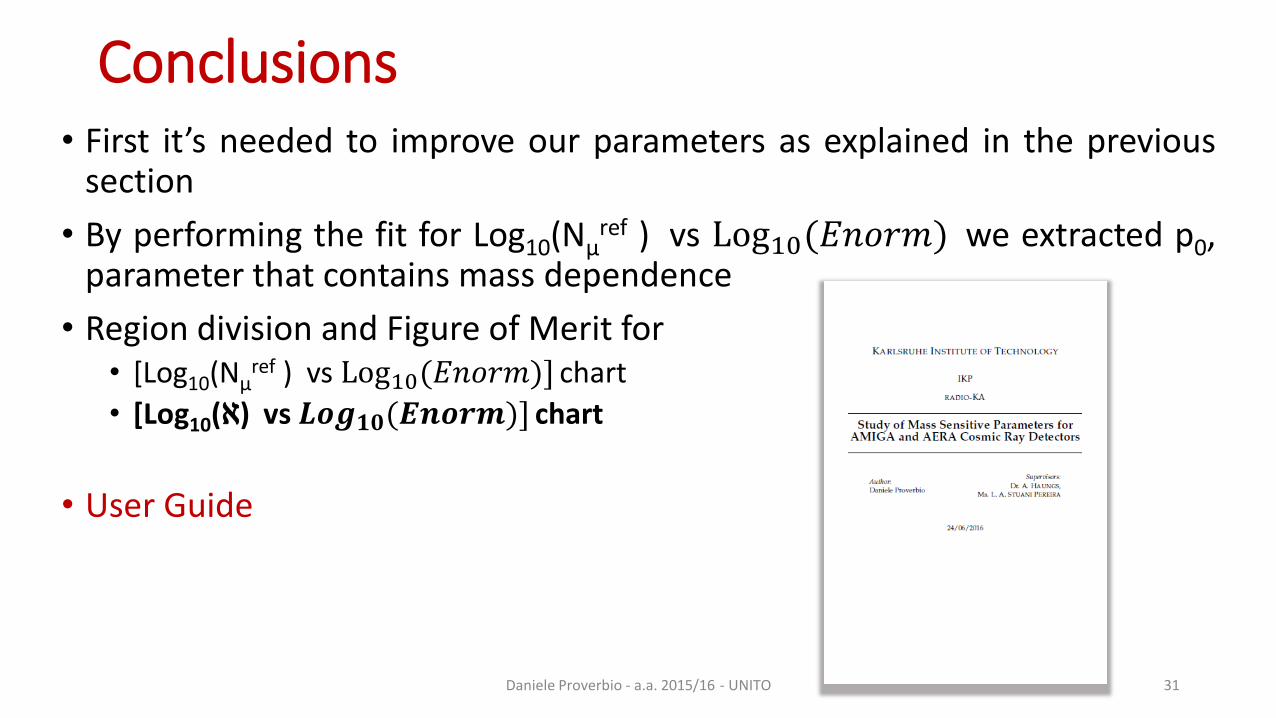
Conclusions• First it’s needed to improve our parameters as explained in the previous

section

• By performing the fit for Log10(Nμref ) vs Log10(𝐸𝑛𝑜𝑟𝑚) we extracted p0,

parameter that contains mass dependence

• Region division and Figure of Merit for• [Log10(Nμ

ref ) vs Log10(𝐸𝑛𝑜𝑟𝑚)] chart

• [Log10(ℵ) vs 𝑳𝒐𝒈𝟏𝟎(𝑬𝒏𝒐𝒓𝒎)] chart

• User Guide


Thanks for your attention


Appendix and Credits


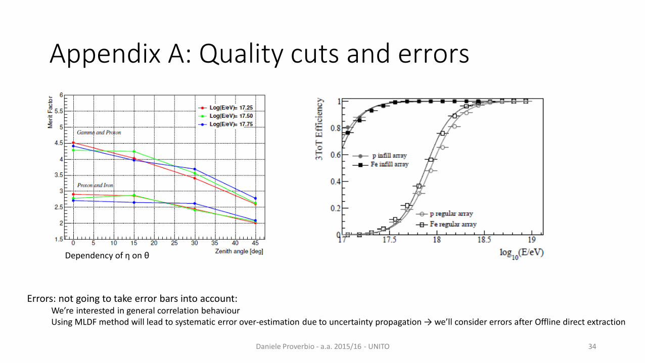
Appendix A: Quality cuts and errors


Dependency of η on θ

Errors: not going to take error bars into account:We’re interested in general correlation behaviourUsing MLDF method will lead to systematic error over-estimation due to uncertainty propagation → we’ll consider errors after Offline direct extraction

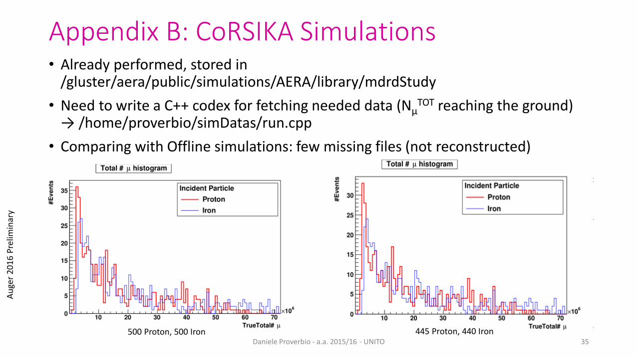
Appendix B: CoRSIKA Simulations• Already performed, stored in

/gluster/aera/public/simulations/AERA/library/mdrdStudy

• Need to write a C++ codex for fetching needed data (NµTOT reaching the ground)

→ /home/proverbio/simDatas/run.cpp

• Comparing with Offline simulations: few missing files (not reconstructed)

Daniele Proverbio - a.a. 2015/16 - UNITO 35500 Proton, 500 Iron 445 Proton, 440 Iron

Au

ger

20

16

Pre

limin

ary

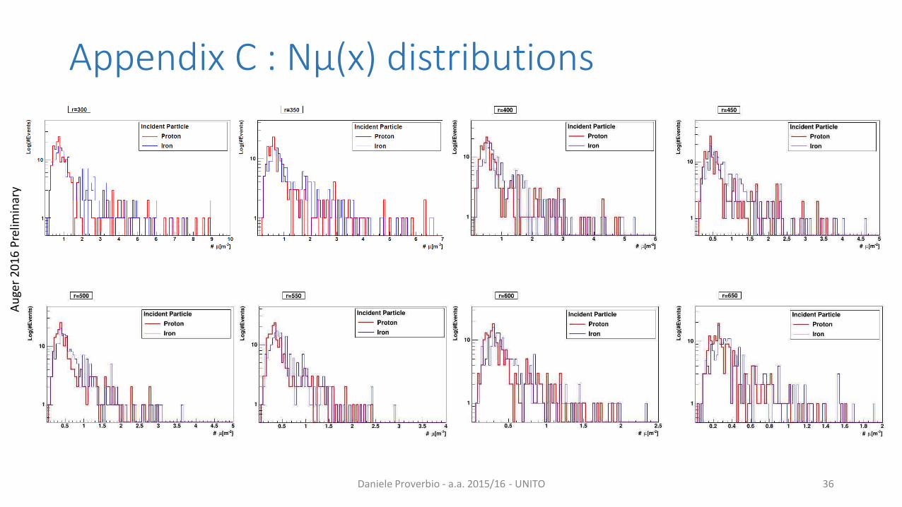
Appendix C : Nμ(x) distributions


Au

ger

2016

Pre

limin

ary

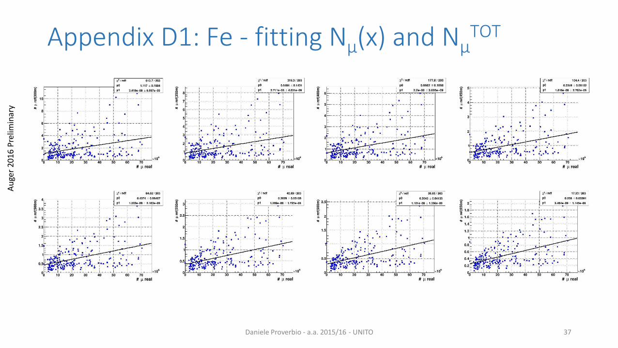
Appendix D1: Fe - fitting Nμ(x) and NμTOT


Au

ger

2016

Pre

limin

ary

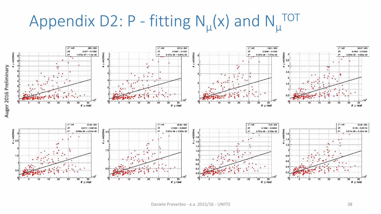
Appendix D2: P - fitting Nμ(x) and NμTOT


Au

ger

2016

Pre

limin

ary

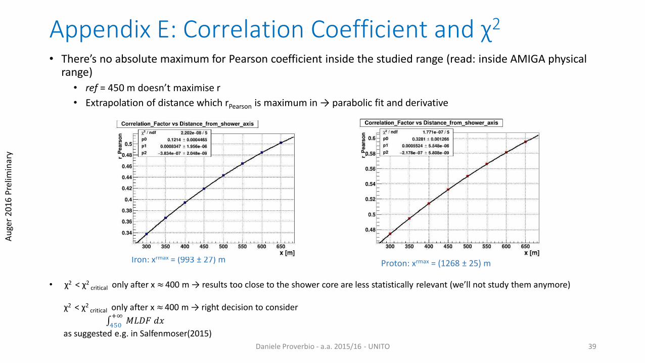
Appendix E: Correlation Coefficient and χ2

• There’s no absolute maximum for Pearson coefficient inside the studied range (read: inside AMIGA physicalrange)

• ref = 450 m doesn’t maximise r

• Extrapolation of distance which rPearson is maximum in → parabolic fit and derivative


Iron: xrmax = (993 ± 27) m Proton: xrmax = (1268 ± 25) m

• χ2 < χ2 critical only after x ≈400 m → results too close to the shower core are less statistically relevant (we’ll not study them anymore)

χ2 < χ2 critical only after x ≈400 m → right decision to consider

450+∞

𝑀𝐿𝐷𝐹 𝑑𝑥

as suggested e.g. in Salfenmoser(2015)

Au

ger

2016

Pre

limin

ary

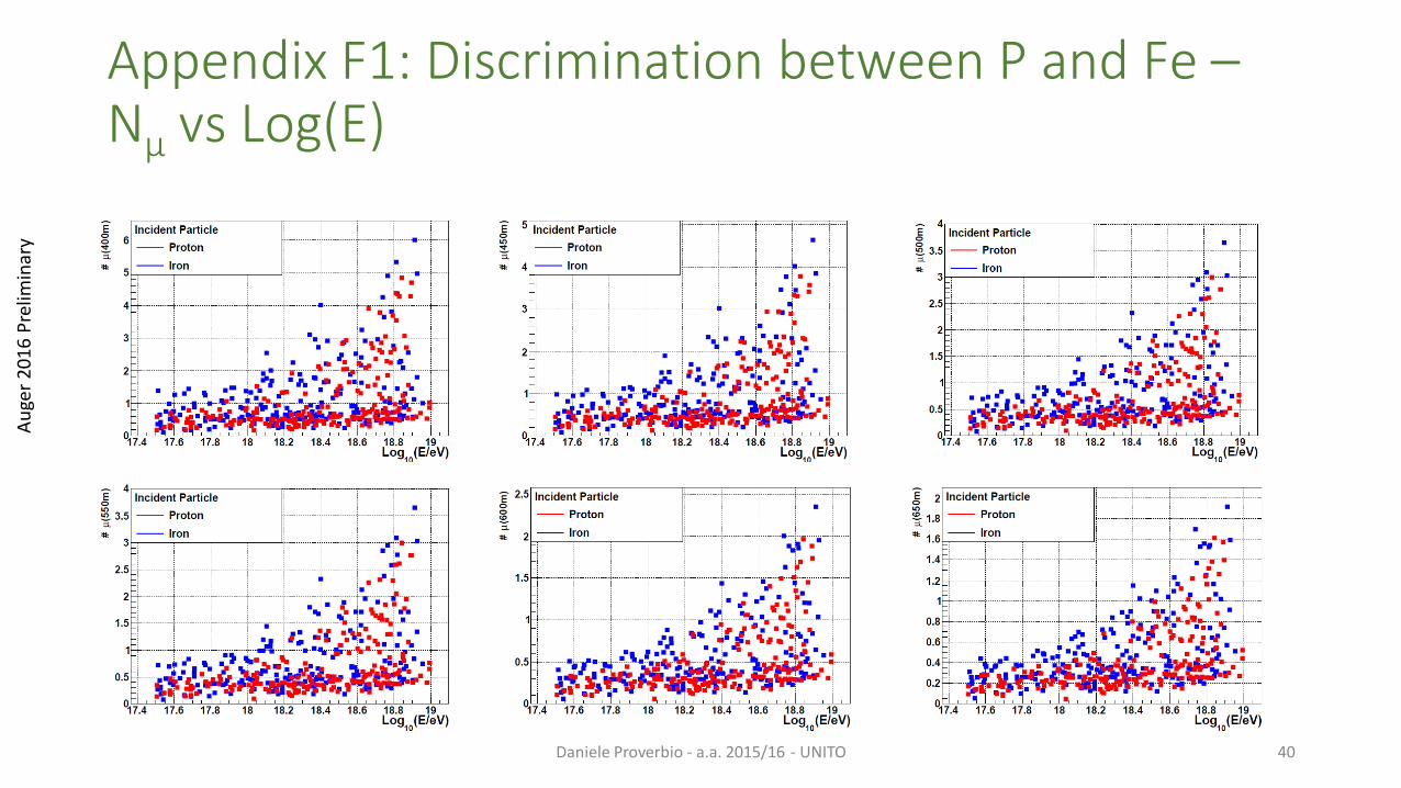
Appendix F1: Discrimination between P and Fe –Nμ vs Log(E)


Au

ger

2016

Pre

limin

ary

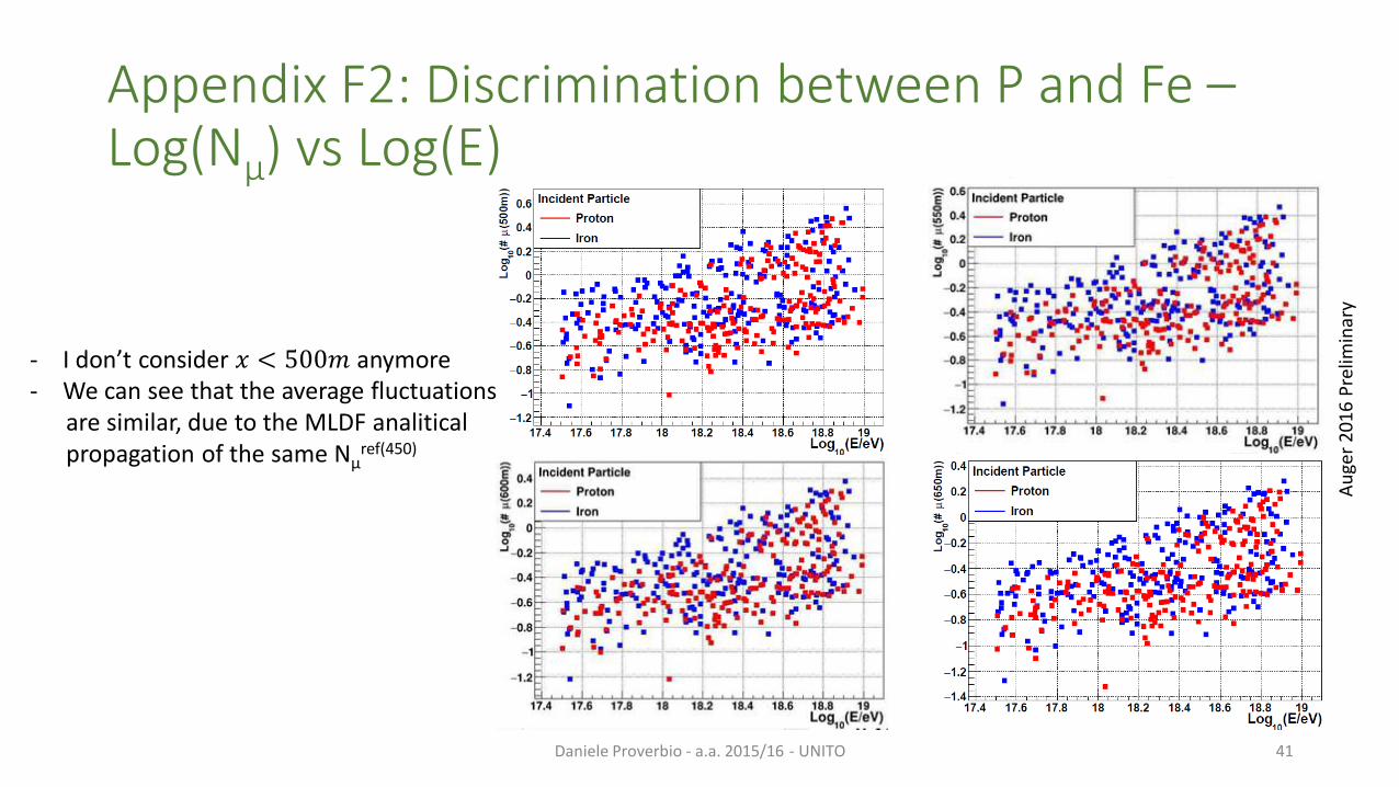
Appendix F2: Discrimination between P and Fe –Log(Nμ) vs Log(E)


- I don’t consider 𝑥 < 500𝑚 anymore- We can see that the average fluctuations

are similar, due to the MLDF analiticalpropagation of the same Nμ

ref(450)

Au

ger

2016

Pre

limin

ary

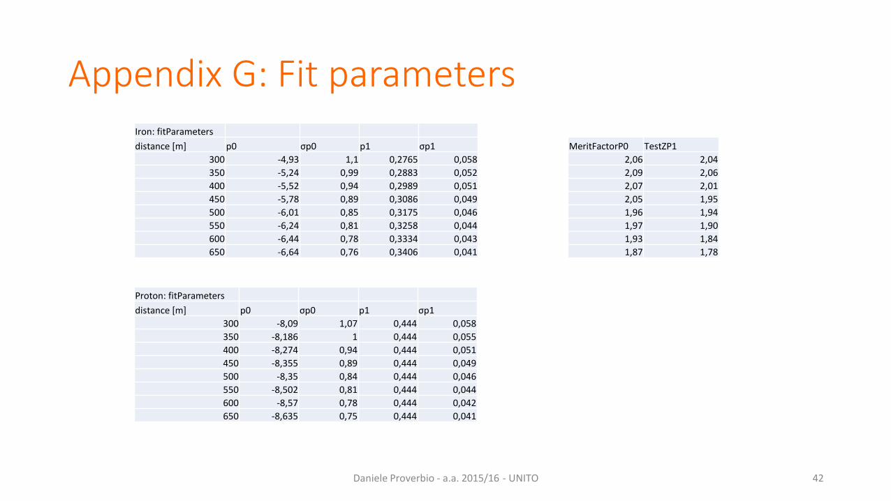
Appendix G: Fit parameters


Proton: fitParameters

distance [m] p0 σp0 p1 σp1

300 -8,09 1,07 0,444 0,058

350 -8,186 1 0,444 0,055

400 -8,274 0,94 0,444 0,051

450 -8,355 0,89 0,444 0,049

500 -8,35 0,84 0,444 0,046

550 -8,502 0,81 0,444 0,044

600 -8,57 0,78 0,444 0,042

650 -8,635 0,75 0,444 0,041

Iron: fitParameters

distance [m] p0 σp0 p1 σp1

300 -4,93 1,1 0,2765 0,058

350 -5,24 0,99 0,2883 0,052

400 -5,52 0,94 0,2989 0,051

450 -5,78 0,89 0,3086 0,049

500 -6,01 0,85 0,3175 0,046

550 -6,24 0,81 0,3258 0,044

600 -6,44 0,78 0,3334 0,043

650 -6,64 0,76 0,3406 0,041

MeritFactorP0 TestZP1

2,06 2,04

2,09 2,06

2,07 2,01

2,05 1,95

1,96 1,94

1,97 1,90

1,93 1,84

1,87 1,78

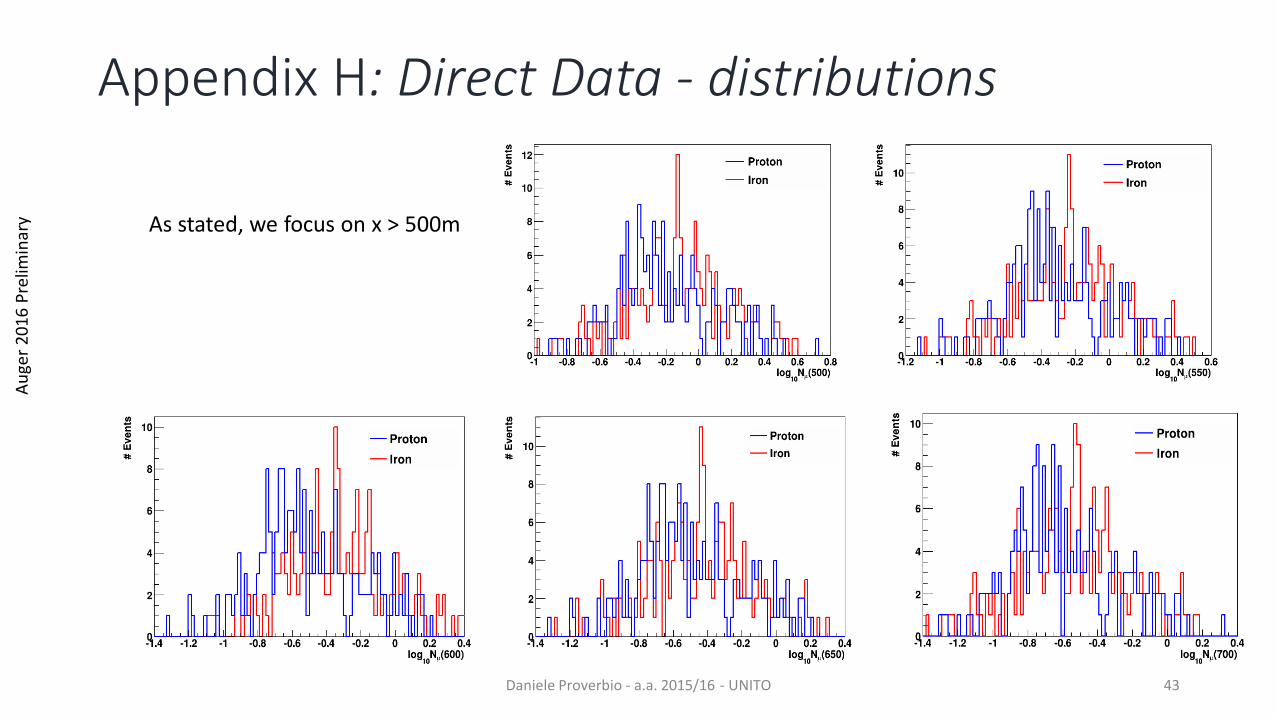
Appendix H: Direct Data - distributions


As stated, we focus on x > 500m

Au

ger

2016

Pre

limin

ary

Appendix I1: Direct Data: Fit


Best

Au

ger

2016

Pre

limin

ary

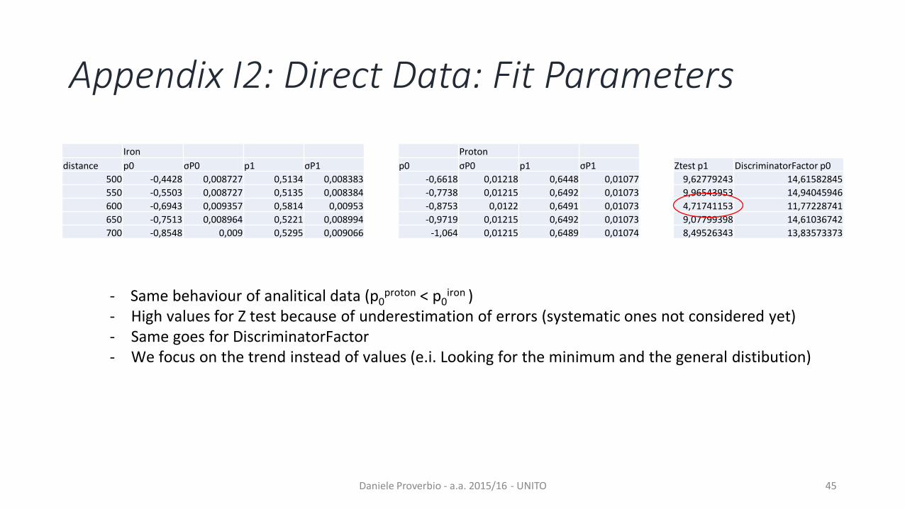
Appendix I2: Direct Data: Fit Parameters

Iron

distance p0 σP0 p1 σP1

500 -0,4428 0,008727 0,5134 0,008383

550 -0,5503 0,008727 0,5135 0,008384

600 -0,6943 0,009357 0,5814 0,00953

650 -0,7513 0,008964 0,5221 0,008994

700 -0,8548 0,009 0,5295 0,009066


Proton

p0 σP0 p1 σP1

-0,6618 0,01218 0,6448 0,01077

-0,7738 0,01215 0,6492 0,01073

-0,8753 0,0122 0,6491 0,01073

-0,9719 0,01215 0,6492 0,01073

-1,064 0,01215 0,6489 0,01074

Ztest p1 DiscriminatorFactor p0

9,62779243 14,61582845

9,96543953 14,94045946

4,71741153 11,77228741

9,07799398 14,61036742

8,49526343 13,83573373

- Same behaviour of analitical data (p0proton < p0

iron )High - values for Z test because of underestimation of errors (systematic ones not considered yet)Same- goes for DiscriminatorFactorWe- focus on the trend instead of values (e.i. Looking for the minimum and the general distibution)

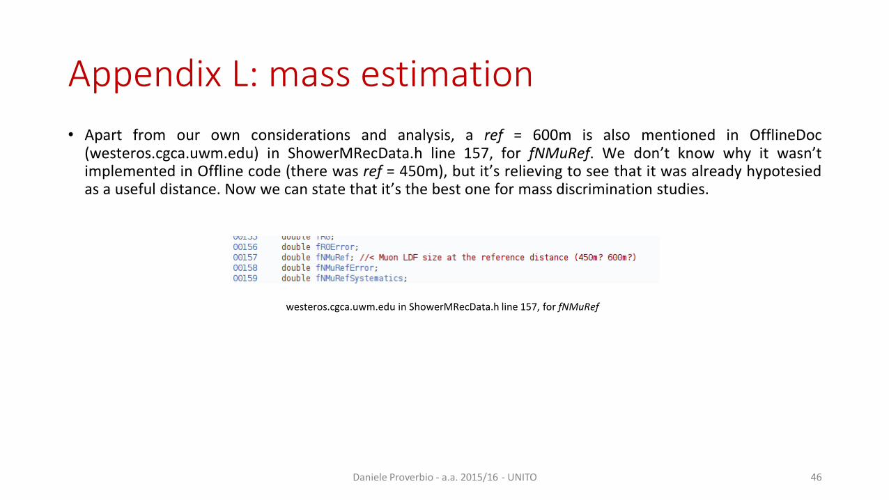
Appendix L: mass estimation

Apart• from our own considerations and analysis, a ref = 600m is also mentioned in OfflineDoc(westeros.cgca.uwm.edu) in ShowerMRecData.h line 157, for fNMuRef. We don’t know why it wasn’timplemented in Offline code (there was ref = 450m), but it’s relieving to see that it was already hypotesiedas a useful distance. Now we can state that it’s the best one for mass discrimination studies.


westeros.cgca.uwm.edu in ShowerMRecData.h line 157, for fNMuRef

Image Credits• [2] Germany Map: https://goo.gl/eWnZNi

• [2] KIT Map: http://goo.gl/ikdJ4a

• [2] Castle: http://goo.gl/0LZdZy

• [4] Spectrum 1: Jansen (2016)

• [4] Spectrum 2: http://goo.gl/qu8VzW

• [5] Air shower profile: Niechciol (2011)

• [5] Shower components: Fuhrmann (2012)

• [7] Electromagnetic effects: Quader Dorosti Hasankiadeh & The Pierre Auger Collaboration, Radio Detection of air shower at the Pierre AugerObservatory, KIT

• [8] Simulated showers: Klepser (2006)

• [9] Pierre Auger Overlook: http://goo.gl/L9sOKq

• [9] Tank in foreground: https://goo.gl/9qrvLG

• [10] LPDA: Neuser (2010)

• [10] AMIGA energy frame: Garilli(2013)

• [10] AMIGA deployment: Niechciol (2011)

• [13] Hybrid measurements: Pierre Auger Collaboration (2016)

• [15] Ewa Holt’s Plots

• [21] MLDF fluctuations: Tapia (2015)

• [34] AMIGA efficiency: Pierre Auger Collaboration (2011)

• [34] Merit Factor Graphic: Tapia (2013)


Essential Bibliography• P. Abreu & al., Advanced functionality for radio analysis in the Offline software framework of the Pierre Auger Observatory, Nuclear Instruments and Methods in

Physics Research A635, 2011, 92–102

• A. A. Al-Rubaiee & al., Study of Cherenkov Light Lateral Distribution Function around the Knee Region in Extensive Air Showers, arXiv:1505.02757 [physics.gen-ph] 6 May 2015

• AugerWiki, The AMIGA extension for the Offline Framework (https://goo.gl/m4EmGK)

• D. Atri, Hadronic interaction models and the angular distribution of cosmic ray muons, arXiv:1309.5874v1 [astro-ph.HE] 23 Sep 2013

• J. Blümer, R. Engel & J. R. Hörandel, Cosmic rays from the knee to the highest energies, Elesevier B.V., 2009, doi:10.1016/j.ppnp.2009.05.002

• I. M. Brancus & al., Features of muon arrival time distributions of high energy EAS at large distances from the shower axis, J. Phys. G: Nucl. Part. Phys. 29 (2003) 453–473

• G.Garilli, Study of the performances of the AMIGA muon detectors of the Pierre Auger Observatory, Università degli Studi di Catania, PhD Thesis, 2013

• K. Greisen, Cosmic Ray Showers, Annu. Rev. Nucl. Sci. 1960.10:63-108. (downloaded from www.annualreviews.org)

• A. Haungs for KASCADE Collaboration, Multifractal moment analysis of the core of PeV air shower for the estimate of the cosmic ray composition, Karlsruhe (arXiv: 10.1.1.8.4816)

• J. R. Hörandel, A review of experimental results at the knee, arXiv:astro-ph/0508014v1 31 Jul 2005

• T. Huege, CoREAS 1.0 User’s Manual, 2013

• S. Jansen, Radio for the Masses - Cosmic ray mass composition measurements in the radio frequency domain, Radboud University Nijmegen, 2016

• K.H. Kampert & M.l Unger, Measurements of the Cosmic Ray Composition with Air Shower Experiments, arXiv:1201.0018v2 [astro-ph.HE] 19 Feb 2012

• S. Klepser, CORSIKA: Extensive Air ShowerSimulation, Humboldt-Universität zu Berlin, 2006

• D. Kostunin & al., Reconstruction of air-shower parameters for large-scale radio detectors using the lateral distribution, arXiv:1504.05083v2 [astro-ph.HE] 18 Dec2015

• J. Neuser, Radio Measurement of Extensive Air Showers at the Pierre Auger Observatory, Bergischen Universität Wuppertal, 2010


Essential Bibliography• B. Sc. M. Niechciol, Muon counter simulation studies for the AMIGA enhancement of the Pierre Auger Observatory, Universität Siegen, 2011

• Pierre Auger Collaboration, Energy Estimation of Cosmic Rays with the Engineering Radio Array of the Pierre Auger Observatory, arXiv:1508.04267v1 [astro-ph.HE] 18 Aug 2015

• Pierre Auger collaboration, Prototype muon detectors for the AMIGA component of the Pierre Auger Observatory, doi:10.1088/1748-0221/11/02/P02012

• Pierre Auger Collaboration, The Pierre Auger Observatory V: Enhancements, 32ND International Cosmic Ray Conference, Beijing 2011

• Pierre Auger Collaboration and J.G. Gonzalez, The Offline Software of the Pierre Auger Observatory: Lessons Learned, arXiv:1208.2154v1 [astro-ph.IM] 10 Aug 2012

• Pierre Auger Collaboration and F. Schröder, Radio detection of high-energy cosmic rays with the Auger Engineering Radio Array, arXiv:1601.00462v1 [astro-ph.IM] 4 Jan 2016

• Pierre Auger Collaboration & F. Suarez, The AMIGA muon detectors of the Pierre Auger Observatory: overview and status, 33RD International cosmic ray conference, Rio de Janeiro 2013

• Pierre Auger Collaboration and E. Varela, The low-energy extensions of the Pierre Auger Observatory, Journal of Physics: Conference Series 468 (2013), doi:10.1088/1742-6596/468/1/012013

• D. Ravignani & A. D. Supanitsky, A new method for reconstructing the muon lateral distribution with an array of segmented counters, arXiv:1411.7649v1 [astro-ph.IM] 27 Nov 2014

• D. Ravignani, A. D. Supanitsky, D. Melo, and B. Wundheiler, A method to reconstruct the muon lateral distribution with an array of segmented counters with time resolution, arXiv:1510.01266v1 [astro-ph.IM] 5 Oct 2015

• L. Salfenmoser, E. Holt, F. Schröder & A. Haungs, A First Combined Analysis of AMIGA and AERA Measurements, GAP 2015-004

• A. D. Supanitsky & al., Underground Muon Counters as a Tool for Composition Analyses, arXiv:0804.1068v2 [astro-ph] 13 Oct 2008

• A. Tapia & al., Study of the chemical composition of high energy cosmic rays using the muon LDF of EAS between 1017.25 eV and 1017.75 eV, arXiv:1501.02217v1 [astro-ph.HE] 9 Jan 2015

• A. Tapia & al., The lateral shower age parameter as an estimator of chemical composition, 33ND International cosmic ray conference, Rio de Janeiro, 2013, arXiv:1309.3536v1 [astro-ph.HE] 13 Sep 2013

• J. Vícha, Analysis of Air Showers with respect to Primary Composition of Cosmic Rays, GAP-2016-025 (2015)


Documents

Studyof mass sensitive parametersfor AMIGA and AERA ...personalpages.to.infn.it/~bertaina/tesi-scaricate/... · Studyof mass sensitive parametersfor AMIGA and AERA cosmicraydetectors