Studyof the preheating phase of chaotic inﬂation

Study of the preheating phase of chaotic inflation

Paul R. Anderson,1,* Carmen Molina-Parıs,2,+ David Evanich,1 and Gregory B. Cook1,‡

1Department of Physics, Wake Forest University, Winston-Salem, North Carolina 27109, USA2Department of Applied Mathematics, School of Mathematics, University of Leeds, Leeds LS2 9JT, United Kingdom

(Received 8 January 2008; published 10 October 2008)

Particle production and its effects on the inflaton field are investigated during the preheating phase of

chaotic inflation using a model consisting of a massive scalar inflaton field coupled to N massless quantum

scalar fields. The effects of spacetime curvature and interactions between the quantum fields are ignored.

A large N expansion is used to obtain a coupled set of equations including a backreaction equation for the

classical inflaton field. Previous studies of preheating using these equations have been done. Here the first

numerical solutions to the full set of equations are obtained for various values of the coupling constant and

the initial amplitude of the inflaton field. States are chosen so that initially the backreaction effects on the

inflaton field are small and the mode equations for the quantum fields take the form of Mathieu equations.

Potential problems relating to the parametric amplification of certain modes of the quantum fields are

identified and resolved. A detailed study of the damping of the inflaton field is undertaken. Some

predictions of previous studies are verified and some new results are obtained.

DOI: 10.1103/PhysRevD.78.083514 PACS numbers: 98.80.Cq, 04.62.+v

I. INTRODUCTION

In all inflationary models there must be a period afterinflation in which a substantial amount of particle produc-tion occurs in order to repopulate the universe with matterand radiation. At the end of this process it is crucial that theuniverse reheats to a temperature that is not too large andnot too small [1]. If the temperature is too large, there areproblems with the creation of monopoles and domain wallsthat have not been observed, and if the temperature is toolow there can be problems with baryogenesis [2]. Thus, toassess the viability of a particular model of inflation, it isnecessary to obtain an accurate picture of the amount ofparticle production that occurs and the rate that it occurs at.This phase of particle production after inflation is usuallycalled reheating [3,4].

Both the mechanism for inflation and the way in whichreheating occurs are different for different inflationarymodels. In both new inflation [5] and chaotic inflation[6], inflation is due to a classical scalar field called theinflaton field. When inflation is over, this field oscillates intime as it effectively ‘‘rolls back and forth’’ in its potential[6–8]. The coupling of this classical field to various quan-tum fields, and in some cases to its own quantum fluctua-tions, results in the production of particles which arethermalized by their mutual interactions. The backreactionof the quantum fields on the classical inflaton field causesits oscillations to damp [1].

The original particle production calculations for newinflation and chaotic inflation [9] were done using pertur-

bation theory. The damping of the inflaton field was takeninto account through the use of a dissipative term that wasadded to its wave equation. Later, the mode equations forthe quantum fields coupled to the inflaton field weresolved, and it was found that the time dependent part ofthe modes can, in some cases, undergo parametric ampli-fication due to the periodic behavior of the inflaton field[10–12]. Since the rate of particle production is extremelyrapid in this case and the particles do not have time tothermalize while it is occurring, this initial phase of theparticle production process was dubbed ‘‘preheating’’ [10].The process of preheating is interesting because particle

production occurs very rapidly with the result that quantumeffects are large and the backreaction on the inflaton field isimportant. This pushes the semiclassical approximation,which is what is typically used in these calculations, to thelimit. In fact, to take such large effects into account it isnecessary to go beyond the ordinary loop expansion. TheHartree approximation and the large N expansion are twoways in which such effects have been treated [13,14].The original calculations of preheating [10,11] involved

solving the mode equations for the quantum fields in thepresence of a background inflaton field which obeyed aclassical scalar field wave equation. Later estimates of theeffects of the quantized fields on the inflaton field weremade using a variety of techniques [15–20]. InRefs. [21,22] the first fully nonlinear calculations of clas-sical inflaton decay were carried out by means of statisticalfield theory lattice numerical simulations. The numericalsimulations in [21] and the later ones in [23–28] wereimplemented by means of the lattice code LATTICEASY

[29]. These simulations are important for the study of thedevelopment of equilibrium after preheating, when scat-tering effects cannot be neglected [23]. Recently, the same

*[email protected][email protected]‡[email protected]

PHYSICAL REVIEW D 78, 083514 (2008)

1550-7998=2008=78(8)=083514(18) 083514-1 � 2008 The American Physical Society

http://dx.doi.org/10.1103/PhysRevD.78.083514

type of calculation has been used to investigate the possi-bility that nonequilibrium dynamics, such as that of para-metric resonance during preheating, can produce non-Gaussian density perturbations [30].

The full set of coupled equations relating the inflatonfield to the quantum fields were solved numerically forboth the Hartree approximation with a single massivescalar field with a quartic self-coupling and the OðNÞmodel using a largeN expansion truncated at leading order.The OðNÞ model consists of N identical massive scalarfields each with a quartic self-coupling and a quadraticcoupling to every other field. As a result there are Ninflaton fields in this model. The first set of calculationswere done in a Minkowski spacetime background [13,31]and then followed by radiation and matter dominatedFriedmann-Robertson-Walker backgrounds [32]. As thefields have an energy-momentum tensor associated withthem, the expansion of the universe is also affected. Thiswas taken into account in Ref. [33]. A numerical calcula-tion in the context of the SU(2) Higgs model was done inRef. [34]. A calculation within the context of the OðNÞmodel that takes scattering of the produced particles intoaccount was done in Ref. [35]. Numerical calculations inmodels with two scalar fields, with backreaction effectstaken into account using the Hartree approximation, weredone in Ref. [36].

There are some potential problems with using the OðNÞmodel as a model for chaotic inflation. One is that it resultsin N inflaton fields rather than the single inflaton field thatis usually postulated. Another is that the fields have aquartic self-coupling as well as couplings to each other.There is evidence from the WMAP III data [37] that ifchaotic inflation occurred, the inflaton field is a massivescalar field with no quartic self-coupling. Finally, in theOðNÞ model or in a model in which the primary quantumfluctuations come from the inflaton field, the quantumfields are massive with the same mass as the inflaton field.However, in a realistic situation there would also be mass-less or effectively massless fields coupled to the inflatonfield.

A possibly more realistic model for chaotic inflationconsists of a single classical inflaton field coupled tovarious quantum fields, including its own quantum fluctu-ations. This is the type of model considered by Kofman,Linde, and Starobinsky [10,11,15]. They used solutions ofthe mode equations of the quantum fields to estimate boththe amount of particle production that would occur invarious cases and the amount of damping of the inflatonfield that occurs due to the backreaction of the quantumfields on it.

In this paper we consider a model similar to the one usedby Kofman, Linde, and Starobinsky, henceforth referred toas KLS, in their analysis of preheating in chaotic inflation[15]. The inflaton field is a classical massive scalar fieldwith minimal coupling to the scalar curvature. It has no

quartic or higher order self-coupling. But it is coupled to Nidentical massless quantized scalar fields with arbitrarycurvature coupling �. As discussed in Sec. II, in the largeN limit, the system effectively reduces to one consisting ofa classical inflaton field coupled to one quantized masslessscalar field with arbitrary curvature coupling. The effectsof quantum fluctuations of the inflaton field come in at nextto leading order so we do not take them into account.We investigate some of the details of the preheating

process by numerically integrating both the mode equa-tions for the quantized field and the backreaction equationfor the inflaton field. These are the first solutions to the fullset of coupled equations relating the inflaton field to thequantum field that have been obtained for this model. Tosimplify the calculations we ignore interactions betweenthe created particles. Calculations that have taken suchinteractions into account [21,22,26,27,35] indicate thatthey can be ignored during the first stages of preheatingbut eventually become important. Another simplification isthat, as a first step, we work in a Minkowski spacetimebackground. It has previously been shown that the expan-sion of the universe can significantly affect the evolution ofthe inflaton field during preheating if this field is of Planckscale or larger at the onset of inflation [15]. This in turn cansubstantially affect the details of the particle creation pro-cess. Thus, some of our results will not be relevant for mostmodels of chaotic inflation. However, for the rapid damp-ing phase which occurs in many models, the amplitude ofthe inflaton field changes rapidly on time scales which aresmall compared to the Hubble time. Thus, it should bepossible to ignore the expansion of the universe during thisphase [15].If, for the model we are considering, one neglects the

backreaction effects of the quantized fields on the inflatonfield, then the inflaton field undergoes simple harmonicmotion with a frequency equal to its mass. As shown inSec. III, this means that the time dependent part of themodes of the quantized field obey a Mathieu equation.Thus, parametric amplification will occur for modes incertain energy bands. There is an infinite number of thesebands, and some occur for arbitrarily large values of theenergy. This could, in principle, result in divergences ofquantities such as h 2i, with the quantum field. Forexample, if the contribution to the mode integral in h 2i[see Eq. (2.11)] for each band of modes undergoing para-metric amplification was the same at a given time, thenh 2i would diverge. Another issue that must be addressedis that even if h 2i is finite, one must be certain that allsignificant contributions to it are accounted for when mak-ing numerical computations; in other words, one must becertain that no important bands are missed. These issuesare addressed in Sec. III.When the backreaction of the quantized fields is in-

cluded in the wave equation for the inflaton field, then, asexpected, the inflaton field’s amplitude damps as the am-

ANDERSON, MOLINA-PARIS, EVANICH, AND COOK PHYSICAL REVIEW D 78, 083514 (2008)

083514-2

plitudes of some of the modes of the quantized field grow.KLS predicted that if all the instability bands are narrowthen the damping is relatively slow, while if one or more ofthe instability bands are wide then there is a period of rapiddamping. We find this to be correct, and for a Minkowskispacetime background, we find a more precise criterionwhich determines whether a phase of rapid damping willoccur. In cases where there is rapid damping, we find asecond criterion that must be satisfied before it takes place.In a Minkowski spacetime background, this latter criterionexplains the differences that are observed in the time that ittakes for the period of rapid damping to begin.

In their study of the rapid damping phase, KLS gave acriterion for when the damping should cease and used it topredict how much damping should occur. We find some-thing similar except that the amount of damping that isobserved to occur is larger than they predict. We also findthat the rapid damping actually occurs in two phasesseparated by a short time. An explanation for this is pro-vided in Sec. IVD.

If most of the damping occurs gradually then it isobserved that the frequency of the oscillations of theinflaton field changes slowly as its amplitude is damped.There is also a significant transfer of energy away from theinflaton field as would be expected. However, if most of thedamping occurs rapidly then during the rapid dampingphase the frequency of the oscillations of the inflaton fieldincreases significantly. As a result there is less energypermanently transferred away from the inflaton field thanmight be otherwise expected. This result was seen previ-ously in the classical lattice simulation of Prokopec andRoos [22].

No significant further damping of the amplitude of theinflaton field was observed to occur after the rapid dampingphase in all cases in which such a phase occurs. Instead,both the amplitude and frequency of the inflaton field wereobserved to undergo periodic modulations and a significantamount of energy was continually transferred away fromand then back to the inflaton field. However, the actualevolution of the inflaton field after the rapid damping phaseis likely to be very different because interactions that weare neglecting are expected to be important during thisperiod [21–23,26,27,35].

In Sec. II the details of our model are given and thecoupled equations governing the inflaton field and thequantum fields are derived. In Sec. III a detailed study ismade of parametric amplification and the bands thatundergo parametric amplification, in order to address theissues discussed above relating to the finiteness of certainquantities and the potential accuracy of numerical compu-tations of these quantities. In Sec. IV some of our numeri-cal solutions to the coupled equations governing the modesof the quantum field and the behavior of the inflaton fieldare presented and discussed. Our results are summarized inSec. V. In the Appendix we provide the details of therenormalization and covariant conservation of the

energy-momentum tensor for the system under considera-tion. Throughout this paper we use units such that @ ¼ c ¼G ¼ 1. The metric signature is ð� þþþÞ.

II. THE MODEL

We consider a single inflaton field � and N identicalscalar fields �j, that represent the quantum matter fields

present during the inflationary phase. We assume that theinflaton field is massive (with mass m) and minimallycoupled to the scalar curvature, R, and that the quantumscalar fields are massless with arbitrary coupling � to thescalar curvature. We also assume that the interaction be-tween the classical inflaton and the quantummatter fields isgiven by g2�2�2

j=2. We study the dynamics of � and �j

in a Minkowski spacetime background and denote themetric by ��.

The action for the system is given by

S½�;�j� ¼ � 1

2

Zd4xð��r��r��þm2�2Þ

� 1

2

XNj¼1

Zd4xð��r��jr��j þ g2�2�2

j Þ:

(2.1)

One can divide the fields into classical and quantum parts

by writing � ¼ �c þ � and �j ¼ with h�i ¼ �c and

h�ji ¼ 0. Then if the inflaton field is rescaled so that�c !ffiffiffiffiN

p�c it is possible to carry out a large N expansion1 using

the closed time path formalism [39]. The result to leadingorder is that the system is equivalent to a two field systemwith the classical inflaton field �c coupled to a single

quantized field , henceforth referred to simply as � and , respectively. The equations of motion for these fields are

ð�hþm2 þ g2h 2iBÞ� ¼ 0; (2.2a)

ð�hþ g2�2Þ ¼ 0; (2.2b)

where h 2iB is the bare (unrenormalized) expectation valueof 2. Restricting to the case of a homogeneous classicalinflaton field in Minkowski spacetime, the equation ofmotion simplifies to

€�ðtÞ þ ðm2 þ g2h 2iBÞ�ðtÞ ¼ 0: (2.3)

Equation (2.2b) is separable and the quantum field ðxÞ canthen be expanded as

ðx; tÞ ¼Z d3k

ð2�Þ3=2 ½akeik�xfkðtÞ þ ayke

�ik�xf�kðtÞ�:(2.4)

The time dependent modes, fkðtÞ, satisfy the following

1The expansion here is similar in nature to one that was carriedout for quantum electrodynamics with N fermion fields inRef. [38].

STUDY OF THE PREHEATING PHASE OF CHAOTIC . . . PHYSICAL REVIEW D 78, 083514 (2008)

083514-3

ordinary differential equation,

€f kðtÞ þ ½k2 þ g2�2ðtÞ�fkðtÞ ¼ 0; (2.5)

and the Wronskian (normalization) condition

fkd

dtf�k � f�k

d

dtfk ¼ i: (2.6)

The WKB approximation for these modes is useful bothfor renormalization and for fixing the state of the field. It isobtained by writing

fkðtÞ ¼ 1ffiffiffiffiffiffiffiffiffiffiffiffiffiffi2WkðtÞ

p exp

��i

Z t

t0

dt0Wkðt0Þ�: (2.7)

Substitution of Eq. (2.7) into Eq. (2.5) gives

W2k ¼ k2 þ g2�2 � 1

2

� €Wk

Wk

� 3

2

_W2k

W2k

�: (2.8)

One solves this equation by iteration. Upon each iterationone obtains a WKB approximation which is higher by twoorders than the previous one. Note that the order dependsboth upon the number of time derivatives and on the power

of g. The zeroth order approximation is just Wð0Þk ¼ k,

while the second order approximation is

Wð2Þk ¼ kþ g2�2

2k; (2.9)

and the fourth order one is

Wð4Þk ¼ kþ g2�2

2k� g4�4

8k3� g2

4k3ð� €�þ _�2Þ: (2.10)

Equation (2.3) for the inflaton field involves the quantityh 2iB. Using (2.4) one finds

h 2iB ¼ 1

2�2

Z þ1

0dkk2jfkðtÞj2: (2.11)

This quantity is divergent and must be regularized. We usethe method of adiabatic regularization [40–43] which, forfree scalar fields in Robertson-Walker spacetimes, has beenshown to be equivalent to the covariant scheme of pointsplitting [44,45].

In adiabatic regularization the renormalization counter-terms are obtained by using a WKB approximation for themodes of the quantized field [42–47]. One works with amassive field and then takes the zero mass limit at the endof the calculation. Expressions for the renormalized valuesof both h 2i and the expectation value of the energy-momentum tensor hT��i for a system similar to the one

we are using2 have been obtained in Ref. [47]. Some details

of the renormalization procedure are given in theAppendix. The result for our system is

h 2iren ¼ 1

2�2

Z �

0dkk2

�jfkðtÞj2 � 1

2k

�

þ 1

2�2

Z þ1

�dkk2

�jfkðtÞj2 � 1

2kþ g2�2

4k3

�þ h 2ian; (2.12a)

h 2ian ¼ � g2�2

8�2

�1� log

�2�

M

��; (2.12b)

where � is a lower limit cutoff that is placed in the integralsthat are infrared divergent andM is an arbitrary parameterwith dimensions of mass which typically appears when themassless limit is taken [46,47]. In principle, the value ofMshould be fixed by observations. For simplicity, we set itequal to the mass of the inflaton field,m, in the calculationsbelow. Note that the value of h 2iren is actually indepen-dent of the value of the infrared cutoff �.It is useful for both the analytic and numerical calcu-

lations to scale the mass of the inflaton field, m, out of theproblem. This can be done by defining new dimensionlessvariables as follows:

�t ¼ mt; (2.13a)

�� ¼ �

m; (2.13b)

�k ¼ k

m; (2.13c)

�fk ¼ffiffiffiffim

pfk; (2.13d)

�M ¼ M

m; (2.13e)

�� ¼ �

m: (2.13f)

If one substitutes h 2iren for h 2iB in Eq. (2.3), writesEqs. (2.3), (2.5), (2.6), and (2.12) in terms of the dimen-sionless variables, rescales h 2iren so that h 2iren !m�2h 2iren, and then drops the bars, the equation for theinflaton field [Eq. (2.3)] becomes

€�ðtÞ þ ½1þ g2h 2iren��ðtÞ ¼ 0; (2.14)

while Eqs. (2.5), (2.6), and (2.12) remain the same. Thesefour equations in terms of the dimensionless variables arethe ones that are solved in the following sections.

III. BACKGROUND FIELD APPROXIMATION

In the background field approximation the wave equa-tion for the inflaton field is solved without taking intoaccount the backreaction effects of the quantum fields onthe inflaton field. However, the effect of the inflaton fieldon the mode equations for the quantum fields is taken intoaccount. For our model the wave equation for the inflatonfield (2.14) then is a simple harmonic oscillator equation,and the mode equation (2.5) is a Mathieu equation.

2In Ref. [47], if the scale factor, aðtÞ, is set equal to 1, thecoupling of the inflaton field to the scalar curvature is set to zero,the coupling constant � is set equal to 2g2, the mass of thequantum field is set to zero, and the ��3=3! term in the equationof motion for the � field is dropped; then the two systems areequivalent.


083514-4

It is well known that for the Mathieu equation there areregions in parameter space for which there are solutionswhich grow exponentially due to a process called para-metric amplification. For the mode equation (2.5) the lastterm is proportional to g2�2

0, with �0 the amplitude of the

oscillations of the inflaton field. Thus, for a given g2�20, it

is the parameter k which determines which modes undergoparametric amplification. There are bands of values of k forwhich this occurs and we shall call them instability bands.The instability band which contains the smallest values ofk will be called the first band.

For a given value of g2�20 there is an infinite number of

instability bands, some of which contain modes with arbi-trarily large values of k. In principle, this could lead todivergences in quantities such as h 2iren and the expecta-tion value of the energy-momentum tensor, hT��iren. Thereason is that, as can be seen from Eq. (2.12a), the renor-malization counterterms do not undergo any exponentialgrowth, while bands of modes with arbitrarily large valuesof k do. One might also be concerned that, even if h 2irenand hT��iren are finite, in order to compute them one must

take into account modes in instability bands with arbi-trarily large values of k. This is clearly not possible forpurely numerical computations, which must necessarilyinclude only a finite number of modes and for which theremust be an ultraviolet cutoff. In this section we use knownproperties of solutions to theMathieu equation to show thatboth h 2iren and hT��iren are finite at any finite time. We

also address the question of how to make sure that thecontributions of all of the instability bands which contrib-ute significantly to h 2iren and hT��iren are included in

numerical calculations of these quantities.

The Mathieu equation

In the background field approximation, without loss ofgenerality (due to time translation invariance), we can takethe solution to Eq. (2.14) to be

�ðtÞ ¼ �0 cosðtÞ: (3.1)

The mode equation is then

€f kðtÞ þ ½k2 þ g2�20cos

2ðtÞ�fkðtÞ ¼ 0: (3.2)

Using the identity

cos 2ðtÞ ¼ 12½1þ cosð2tÞ�; (3.3)

the mode equation can be put into a standard form for theMathieu equation[48]

d2fkðtÞdt2

þ ½a� 2q cosð2tÞ�fkðtÞ ¼ 0; (3.4)

with

a ¼ k2 þ 12g

2�20; (3.5a)

q ¼ �14g

2�20: (3.5b)

Floquet’s theorem applies to the Mathieu equation [49].It implies the existence of two solutions of Eq. (3.4) of theform

f1ðtÞ ¼ e�th1ðtÞ; (3.6)

f2ðtÞ ¼ e��th2ðtÞ; (3.7)

where h1ðtÞ and h2ðtÞ are periodic functions of period 2�,and � is, in general, a complex number [49]. If � has anonvanishing real part, it is easy to see that one solutionwill grow exponentially at late times.Our goal is to find which ranges of values of k lead to

exponentially growing modes. This can be accomplishedby first fixing the value of q and then finding the values ofthe parameter a for which the Mathieu equation has solu-tions with � ¼ 0. Those values of a which correspond toeven solutions are traditionally labeled ar, and those whichcorrespond to odd solutions are labeled br, with r a positiveinteger. The pattern of instability and stability regions inthe ða; qÞ plane is symmetric about q ¼ 0. Thus, for sim-plicity we shall consider q > 0 in what follows, eventhough q < 0 for the equations we are concerned with[see Eq. (3.5b)]. For q > 0, it is found that �2 > 0 forvalues of a which are between ar and br for the same valueof r [48]. Further, one has the relation a0 < b1 < a1 <b2 < . . . .For the purpose of assessing the contribution of unstable

modes with large values of k to Eq. (2.12), it is necessary toknow both the range of values of k in the unstable bandsand the maximum value of � in a band containing largevalues of k. The ranges of k in the large r limit are given bythe relation [50]

ar � br ¼ O

�qr

rr�1

�: (3.8)

Thus, for fixed q, the width of the unstable bands in theða; qÞ plane becomes arbitrarily small for bands with largevalues of r and therefore becomes arbitrarily small forlarge values of k. This means that for unstable modes atlarge values of k to contribute significantly to the integralsin Eq. (2.12), it would be necessary that these modes growmuch faster than the unstable modes in bands with smallervalues of k, which are wider.An approximation to the value of � in unstable bands is

[48]

�2r ¼ ðar þ br � 2a� 4r2Þ

2

�ffiffiffiffiffiffiffiffiffiffiffiffiffiffiffiffiffiffiffiffiffiffiffiffiffiffiffiffiffiffiffiffiffiffiffiffiffiffiffiffiffiffiffiffiffiffiffiffiffiffiffiffiffiffiffiffiffiffiffiffiffiffiffiffiffiffiffiffiffiffiffiffiffiffiffiffiffiffiffiffiffiffiffiffiffiffiffiffiffiffiffiffiffiffia2r � 2arbr � 8r2ðar þ br � 2aÞ þ b2r þ 16r4

p2

;

(3.9)


083514-5

where the boundaries of the unstable band of index r aregiven by the pair of eigenvalues br and ar with ar > br.Some details of the derivation of this approximation can befound in Ref. [51]. Note that there are two possible solu-tions for�r for fixed values of r and a. Given that for larger the instability bands become narrower, and that br � a �ar, it is easy to show that for large r only the plus sign gives�2r > 0. It is also easy to show that

j2a� ar � brj � 4r2; (3.10)

and thus that

�r ’ ½ðar � aÞða� brÞ�1=22r

: (3.11)

For this approximation the maximum value of �r is at themidpoint between br and ar. Since, for large r the width ofthe band, ar � br, gets very small [see Eq. (3.8)], it is clearthat the maximum value of� in a band is smaller for bandswith very large values of k than for bands with smallervalues of k.

The relative contribution of unstable modes to the inte-gral in Eq. (2.12) at a given time t depends in part on howmuch they have grown compared to unstable modes inlower bands. It is clear from the above analysis that modesin higher bands grow significantly slower than those inlower bands. Also for a given time t, there will be somevalue, k ¼ K, for which unstable bands with larger valuesof k have not grown much at all. This, coupled with the factthat the widths of the unstable bands get narrower at largervalues of k, means that at any given time t the modes inbands with k > K will not contribute significantly to themode integral in Eq. (2.12). Thus, h 2iren and hT��iren arefinite.

From the above analysis it should be clear that in nu-merical computations it is possible to obtain a good ap-proximation to h 2iren and hT��iren by putting in a cutoff atsome large value of k. Since the location of the bands atsmall values of k can be determined using standard tech-niques [48], then one simply needs to use a high enoughdensity of modes so that those bands with smaller values ofk are adequately covered.

The maximum value of � occurs for the first unstableband which has the smallest values of k. Once the modes inthis band have become sufficiently large, they make themajor contribution to h 2iren and hT��iren.

IV. BACKREACTION ON THE INFLATON FIELD

A. Initial conditions

A FORTRAN program was written to simultaneouslysolve the mode equations for the field, compute thequantity h 2iren, and solve the equation for the inflatonfield � in terms of the dimensionless variables (2.13). Forthis program to run, initial values must be given for � andits first time derivative, as well as each mode function fk

and its first time derivative. Since the inflaton field is in itsrapid oscillation phase, what is important is the initialamplitude of its oscillations. This is most easily obtained

by starting with �ð0Þ ¼ �0 and _�ð0Þ ¼ 0.The initial values for the mode functions of the field

are determined by the state of the field. As the quantumfield is coupled to the inflaton field, there is no preferredvacuum state. Instead, one can use an adiabatic vacuumstate. Such states have been discussed in detail for cosmo-logical spacetimes [52]. They are based on the WKBapproximation for the modes. It is necessary to choose astate that is of adiabatic order two or higher for the renor-malized value of h 2i to be finite. For the renormalizedenergy-momentum tensor hT��i to be finite, it is necessaryto have at least a fourth order adiabatic state. For such astate, in the large k limit,

jfkj2 ! 1

2k� g2�2

4k3þ 3g4�4

16k5þ g2ð _�2 þ� €�Þ

8k5þOðk�6Þ:

(4.1)

Although the large k behavior of an adiabatic state of agiven order is constrained by requiring that renormaliza-tion of the energy-momentum tensor be possible, there areno such constraints on modes with smaller values of k.Thus, one can construct fourth order adiabatic states thatwould give virtually any value for h 2iren or hT��iren at

some initial time t. However, if the value of g2h 2iren is toolarge at the beginning of preheating, then backreactioneffects will be important immediately. In fact, ifg2h 2iren � 1, then backreaction effects are so stronginitially that parametric amplification is unlikely to occur.If g2h 2iren 1, backreaction effects will be important, butit is possible that parametric amplification might still oc-cur. On the other hand, if g2h 2iren � 1 at the onset ofpreheating, then backreaction effects are not importantinitially and parametric amplification will occur. Sinceour goal is to study the preheating process in detail, werestrict attention to this latter case.A natural way to construct a fourth order adiabatic state

is by using a fourth order WKB approximation to fix the

initial values of the modes, fk, and their derivatives, _fk, forall values of k. For the numerical calculations done in thispaper, the state used was an adiabatic vacuum state with

fkðt ¼ 0Þ ¼ffiffiffiffiY

2

s; (4.2a)

_fkðt ¼ 0Þ ¼ � iffiffiffiffiffiffi2Y

p ; (4.2b)

Y ¼ 1

�0

þ g2�0€�0

4�50

; (4.2c)

�0 ¼ffiffiffiffiffiffiffiffiffiffiffiffiffiffiffiffiffiffiffiffiffiffik2 þ g2�2

0

q: (4.2d)

It is easy to show that this is a fourth order adiabatic state


083514-6

by recalling that _�ð0Þ ¼ 0. The initial values have beenchosen in part to make it possible to analytically computethe initial value of h 2iren, and in part so that theWronskian condition (2.6) is satisfied exactly. For thefourth order adiabatic state that we are using, at the initialtime t ¼ 0

g2h 2ðt ¼ 0Þiren ¼ g2 €�0

48�2�0

� g4�20

16�2

�1� log

�g2�2

0

M2

��:

(4.3)

Using this initial value for g2h 2iren one finds that the

initial value for €�ðtÞ is€�ðt ¼ 0Þ ¼ 1

1þ g2

48�2

��1þ g4�2

0

16�2

�1� log

�g2�2

0

M2

��0:

(4.4)

Thus, whether backreaction effects are important initiallydepends on the values of both�0 and g. For the values of g

considered here, g2

48�2 � 1. From Eq. (4.4) it can be seen

that backreaction effects for the states we are consideringare likely to be important if

g2ðg2�20Þ * 16�2: (4.5)

As an example, for realistic models of chaotic inflation,KLS [15] chose

m ¼ 10�6Mp; �0 ¼Mp

5m: (4.6)

The values they used for g range from10�4 to 10�1. Forg ¼ 10�4, g2�2

0 ¼ 400, while for g ¼ 10�1, g2�20 ¼ 4

108. Applying the criterion (4.5) one finds that our fourthorder adiabatic states result in significant backreactioninitially for these values of m and �0 if g * 8 10�3.

B. Parametric amplification with backreaction

If the initial conditions are such that g2h 2iren � 1, thenexamination of Eq. (2.14) shows that there is no significantbackreaction at early times, and the solution of the inflatonfield will be approximately equal to Eq. (3.1). When,primarily through parametric amplification of certainmodes, g2h 2iren 1, one expects backreaction effects tobe important and to make the amplitude of the oscillationsof the inflaton field, �, decrease. It has been observed inthe numerical computations that h 2iren oscillates about anaverage value which changes in time. The effective mass ofthe inflaton field can be defined in terms of this averagevalue:

m2eff ¼ 1þ g2h 2iren: (4.7)

It is clear that an increase in m2eff results in an increase of

the frequency of oscillations of �. This should happenslowly at first, so one would expect the basic character ofthe mode equation (2.5) to be a Mathieu equation, except

that the effective value of q would change [15]. A zerothorder WKB analysis of the solutions to Eq. (2.14) showsthat the effective frequency of oscillations can be approxi-mated by

!eff � 1

t2 � t1

Z t2

t1

dtffiffiffiffiffiffiffiffiffiffiffiffiffiffiffiffiffiffiffiffiffiffiffiffiffiffiffiffi1þ g2h 2iren

q; (4.8)

with t1 < t < t2 for some time interval t2 � t1 equal to orlarger than an oscillation period of the inflaton field. Aderivation similar to that at the beginning of Sec. III thenshows that

aeff � k2

!2eff

þ 2qeff ; (4.9a)

qeff � g2A2

4!2eff

; (4.9b)

where A is the amplitude of the inflaton field and we havedefined qeff so that it is positive.3 As the inflaton fieldevolves, A will tend to slowly decrease and !eff will tendto slowly increase. Thus, the resulting changes in theinstability bands should be small enough that there wouldbe no problem in having enough modes to accuratelydetermine the primary contributions to h 2iren. Our nu-merical work described below seems to bear this out.Once the backreaction is significant, it is possible for the

character of the equation to change substantially. If �varies in a periodic manner, then it is still possible forparametric amplification to occur due to Floquet’s theorem[49]. It would be difficult in this more complicated situ-ation to analyze the behavior of the solutions to the extentthat solutions to the Mathieu equation have been analyzed.However, it seems quite likely that, as for the Mathieuequation, the most important instability bands will be atrelatively small values of k, and that if an instability band isextremely narrow, then it probably will not have a largeeffect on h 2iren for a very long time. It is likely thatinteractions which are neglected in our model will beimportant on such long time scales [21–23,26,27,35].

C. Some numerical results

Since the mode equation (2.5) depends on g2�2 and theequation of motion of the inflaton field (2.14) depends ong2h 2iren, one would expect that the effects of the values ofg and g2�2

0 decouple, at least to some extent. As can be

seen in Figs. 1 and 2 this is the case, with the quantity g2�20

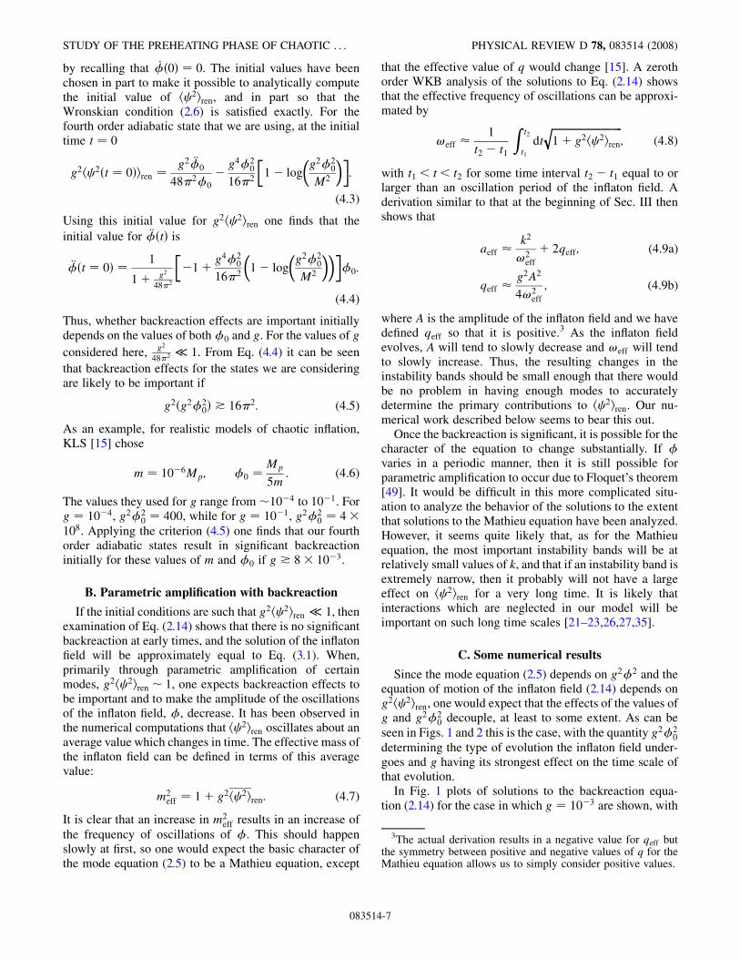
determining the type of evolution the inflaton field under-goes and g having its strongest effect on the time scale ofthat evolution.In Fig. 1 plots of solutions to the backreaction equa-

tion (2.14) for the case in which g ¼ 10�3 are shown, with

3The actual derivation results in a negative value for qeff butthe symmetry between positive and negative values of q for theMathieu equation allows us to simply consider positive values.


083514-7

g2�20 ranging from 35 to 1. For the first two plots most of

the damping occurs over a very short period. After that, thefield does not appear to damp significantly. Instead, itcontinues to oscillate but with a much higher frequencythan before. The envelope of its oscillations also oscillates

but with a much smaller frequency. This behavior has beenobserved for all cases investigated with g2�2

0 * 2.Conversely, for the plot on the bottom (g2�2

0 ¼ 1), it isclear that the damping is much slower and occurs over amuch longer period of time. This behavior is a verification

FIG. 2. The evolution of the inflaton field for g2�20 ¼ 10. The plot on the left is for g ¼ 10�2 and the one on the right is for 10�3.

FIG. 1. The evolution of the inflaton field for g ¼ 10�3. From left to right the top plots are for g2�20 ¼ 35 and 10. The bottom plot is

for g2�20 ¼ 1.


083514-8

of the prediction by KLS [15] that a period of rapid damp-ing would occur for g2�2

0 � 1 and that only relatively

slow damping occurs for g2�20 � 1. A detailed analysis of

the evolution of the inflaton field is given in Sec. IVD.In Fig. 2 plots of solutions to the backreaction equation

for the case in which g2�20 ¼ 10 and g ¼ 10�2 and 10�3

are shown. The amount of damping does not appear todepend in any strong way upon the value of the couplingconstant g. The amount of time it takes for significantdamping to begin is longer for the smaller value of g.This is easily explained by the fact that initiallyg2h 2iren � 1, so that only negligible damping of theinflaton field occurs at early times. During this period themode equations, and thus the growth of h 2iren, is approxi-mately independent of the value of g. Significant back-reaction begins to occur when g2h 2iren 1, and this willobviously take longer for smaller values of g, since h 2irenwill have to grow larger before it can occur.

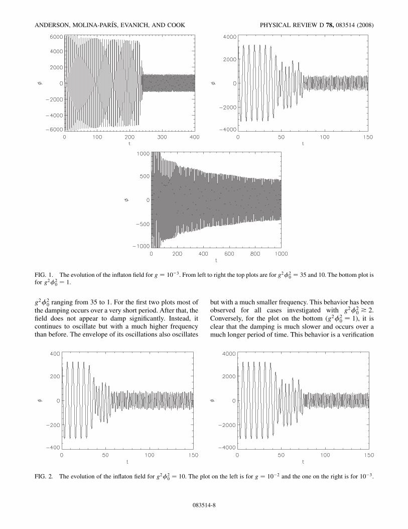
The natural explanation for what is happening in all ofthese cases is that particle production occurs and the back-reaction of the produced particles on the inflaton fieldcauses its amplitude to be damped. However, if this pictureis correct, then one would expect that a significant amountof energy would be transferred from the inflaton field to themodes of the quantum field. To check this, one can com-pute the time evolution of the energy density of the inflatonfield. Since the gravitational background is Minkowskispacetime, the energy density is conserved as is shownexplicitly in the Appendix. As is also shown in theAppendix, the energy density can be broken into twodifferent contributions. The first one is the energy densitythe inflaton field would have if there was no interaction(g ¼ 0). It is given by

� ¼ 12ð _�2 þm2�2Þ: (4.10)

The other contribution is the energy density of the quantum

field shown in Eq. (A6c). It contains terms that would bethere if there was no interaction along with terms thatexplicitly depend on the interaction. This split is usefulbecause almost all of the energy is initially in the inflatonfield, and thus, one can clearly see how much has beentransferred to the quantum field and to the interactionbetween the two fields as time goes on.In Fig. 3 the left-hand plot shows the evolution of the

energy density of the inflaton field for the case g ¼ 10�3

and g2�20 ¼ 1. Comparison with the bottom plot in Fig. 1

shows that as the inflaton field is damped, a large portion ofits energy is permanently transferred away from it.For all cases investigated in which rapid damping of the

inflaton field occurs, it was found that much less energy ispermanently transferred away from the inflaton field thanone might expect, given the amount by which its amplitudehas been damped. This effect was seen previously in theclassical lattice simulation of Prokopec and Roos [22]. Anexample is the case g ¼ 10�3, g2�2

0 ¼ 10 for which the

evolution of the energy density of the inflaton field isshown in the plot on the right panel of Fig. 3.Comparison with the top right plot of Fig. 2 shows thatafter the rapid damping has finished, the inflaton fieldpermanently loses some energy because the maximum ofits energy density is lower than before, but more than halfof the original energy is transferred back and forth betweenthe inflaton field, the quantum field, and the interactionbetween the two. However, it is important to note that incases in which rapid damping occurs, our results cannot betrusted after the rapid damping phase has finished because,as previously mentioned, there is evidence that the inter-actions we neglect become important [21–23,26,27,35].Another effect that was observed to occur in all cases in

which the inflaton field undergoes rapid damping is anextreme sensitivity to initial conditions. If the initial con-ditions are changed by a small amount, then initially the

FIG. 3. The evolution of the energy density of the inflaton field, �. Both plots are for g ¼ 10�3. The one on the left is for g2�20 ¼ 1

and the one on the right is for g2�20 ¼ 10.


083514-9

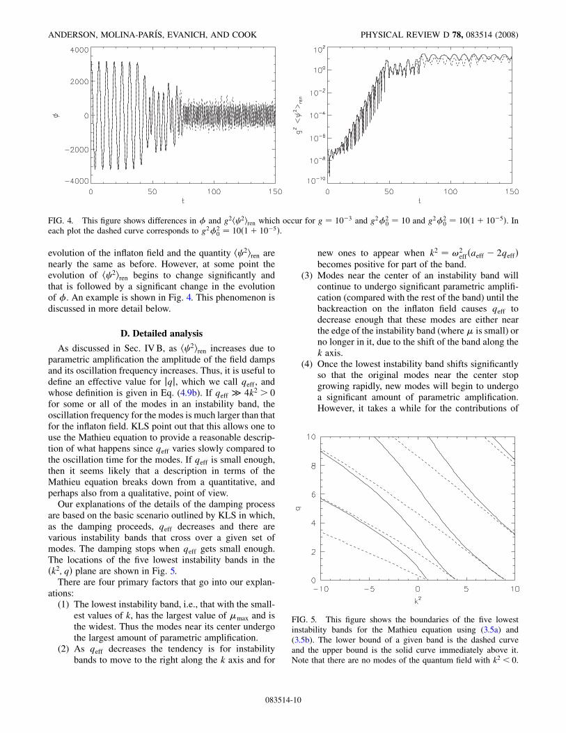
evolution of the inflaton field and the quantity h 2iren arenearly the same as before. However, at some point theevolution of h 2iren begins to change significantly andthat is followed by a significant change in the evolutionof �. An example is shown in Fig. 4. This phenomenon isdiscussed in more detail below.

D. Detailed analysis

As discussed in Sec. IVB, as h 2iren increases due toparametric amplification the amplitude of the field dampsand its oscillation frequency increases. Thus, it is useful todefine an effective value for jqj, which we call qeff , andwhose definition is given in Eq. (4.9b). If qeff � 4k2 > 0for some or all of the modes in an instability band, theoscillation frequency for the modes is much larger than thatfor the inflaton field. KLS point out that this allows one touse the Mathieu equation to provide a reasonable descrip-tion of what happens since qeff varies slowly compared tothe oscillation time for the modes. If qeff is small enough,then it seems likely that a description in terms of theMathieu equation breaks down from a quantitative, andperhaps also from a qualitative, point of view.

Our explanations of the details of the damping processare based on the basic scenario outlined by KLS in which,as the damping proceeds, qeff decreases and there arevarious instability bands that cross over a given set ofmodes. The damping stops when qeff gets small enough.The locations of the five lowest instability bands in theðk2; qÞ plane are shown in Fig. 5.

There are four primary factors that go into our explan-ations:

(1) The lowest instability band, i.e., that with the small-est values of k, has the largest value of �max and isthe widest. Thus the modes near its center undergothe largest amount of parametric amplification.

(2) As qeff decreases the tendency is for instabilitybands to move to the right along the k axis and for

new ones to appear when k2 ¼ !2effðaeff � 2qeffÞ

becomes positive for part of the band.(3) Modes near the center of an instability band will

continue to undergo significant parametric amplifi-cation (compared with the rest of the band) until thebackreaction on the inflaton field causes qeff todecrease enough that these modes are either nearthe edge of the instability band (where� is small) orno longer in it, due to the shift of the band along thek axis.

(4) Once the lowest instability band shifts significantlyso that the original modes near the center stopgrowing rapidly, new modes will begin to undergoa significant amount of parametric amplification.However, it takes a while for the contributions of

FIG. 4. This figure shows differences in � and g2h 2iren which occur for g ¼ 10�3 and g2�20 ¼ 10 and g2�2

0 ¼ 10ð1þ 10�5Þ. Ineach plot the dashed curve corresponds to g2�2

0 ¼ 10ð1þ 10�5Þ.

FIG. 5. This figure shows the boundaries of the five lowestinstability bands for the Mathieu equation using (3.5a) and(3.5b). The lower bound of a given band is the dashed curveand the upper bound is the solid curve immediately above it.Note that there are no modes of the quantum field with k2 < 0.


083514-10

these new modes to the value of h 2iren to becomesignificant compared with that of the modes whichwere previously near the center of the first instabilityband, and have now stopped undergoing significantparametric amplification.

In what follows we first discuss the case in which nosignificant amount of rapid damping occurs. For the casesin which rapid damping does occur, the pre-rapid damping,rapid damping, and post-rapid damping phases are dis-cussed separately.

1. g2�20 & 1

KLS predict and we observe that there is no significantamount of rapid damping for g2�2

0 & 1. However, the

details are different because they consider an expandinguniverse. In the Minkowski spacetime case, as can be seen

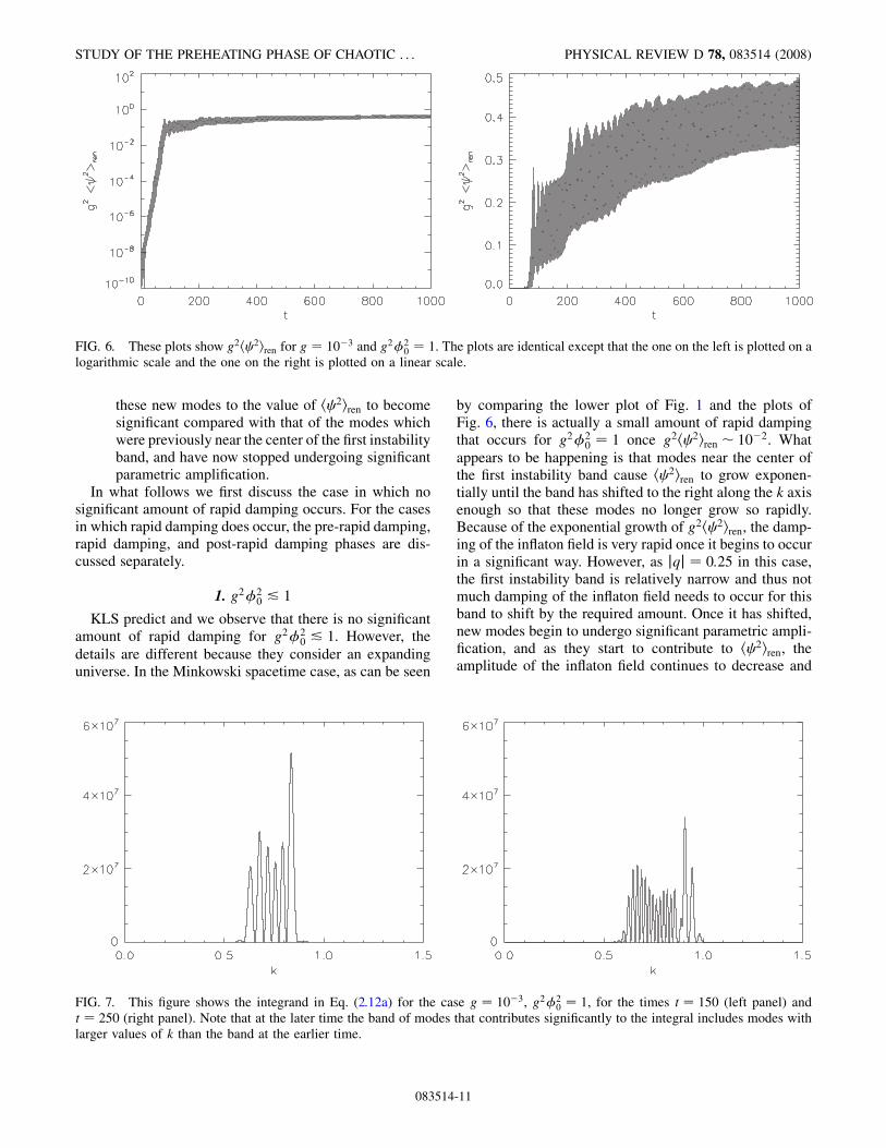
by comparing the lower plot of Fig. 1 and the plots ofFig. 6, there is actually a small amount of rapid dampingthat occurs for g2�2

0 ¼ 1 once g2h 2iren 10�2. What

appears to be happening is that modes near the center ofthe first instability band cause h 2iren to grow exponen-tially until the band has shifted to the right along the k axisenough so that these modes no longer grow so rapidly.Because of the exponential growth of g2h 2iren, the damp-ing of the inflaton field is very rapid once it begins to occurin a significant way. However, as jqj ¼ 0:25 in this case,the first instability band is relatively narrow and thus notmuch damping of the inflaton field needs to occur for thisband to shift by the required amount. Once it has shifted,new modes begin to undergo significant parametric ampli-fication, and as they start to contribute to h 2iren, theamplitude of the inflaton field continues to decrease and

FIG. 7. This figure shows the integrand in Eq. (2.12a) for the case g ¼ 10�3, g2�20 ¼ 1, for the times t ¼ 150 (left panel) and

t ¼ 250 (right panel). Note that at the later time the band of modes that contributes significantly to the integral includes modes withlarger values of k than the band at the earlier time.

FIG. 6. These plots show g2h 2iren for g ¼ 10�3 and g2�20 ¼ 1. The plots are identical except that the one on the left is plotted on a

logarithmic scale and the one on the right is plotted on a linear scale.


083514-11

the position of the instability band continues to moveslowly to the right along the k axis. One can see evidenceof this shift by comparing plots of the integrand for h 2irenat two different times, as is done in Fig. 7.

As the inflaton field continues to damp and qeff contin-ues to decrease, the value of � at the center of the bandshould also be decreasing. Thus, the time scale for the newmodes undergoing parametric amplification to contributesignificantly to the damping increases and the rate ofdamping decreases.

2. g2�20 * 2

For g2�20 * 2 rapid damping has occurred in every case

that has been numerically investigated. However, the timesat which the rapid damping occurs, and the details relatingto both how the rapid damping occurs and how muchdamping there is, vary widely. To understand the reasonsfor this, it is useful to break the discussion up into the pre-rapid damping, rapid damping, and post-rapid dampingphases.

a. Pre-rapid damping phase.—Since g2h 2iren � 1 ini-tially for all cases considered in this paper, there is nosignificant amount of backreaction on the inflaton field atfirst. Therefore, parametric amplification of the modes nearthe center of the first instability band, i.e., the one whichencompasses the smallest values of k, occurs and thecontribution of these modes quickly dominates all othercontributions to h 2iren.4 (As mentioned previously this isin contrast to the case of an expanding universe where theexpansion causes a decrease in the amplitude of the in-flaton field and thus in qeff .) As before, h 2iren growsexponentially until it becomes of order 10�2, at whichpoint significant damping of the inflaton field begins tooccur. What happens next is observed to depend upon thelocation on the k axis of the first instability band.

(1) If k2 < 0 for a significant fraction of the band andk2 > 0 for a significant fraction, then the inflatonfield goes directly into the rapid damping phasewhich is discussed next. A good example of this isthe case g2�2

0 ¼ 10 which is shown in Fig. 4. The

average value of g2h 2i increases exponentially un-til it gets large enough to significantly affect theinflaton field and cause the first phase of rapiddamping to occur. Thus there is no significantamount of gradual damping that occurs before therapid damping phase.

(2) If k2 > 0 for most or all of the band, then as qeffdecreases, the shift in the band causes the modesnear the center to stop increasing rapidly in ampli-tude. In that case the exponential increase in h 2iren

ceases. At this point there are two possibilities thathave been observed:

(a) If the decrease in qeff has resulted in k2 > 0 for partor all of an instability band in the ða; qÞ plane forwhich previously k2 < 0, then the modes which arenow in that band will begin to increase in amplitudeexponentially and will do so at a faster rate thanmodes in what was previously the first instabilityband.

(b) If the decrease in qeff is not large enough for a newinstability band to appear, then slow damping willstart to occur due to parametric amplification ofthose modes that are now near the center of the firstinstability band but which were not close to it be-fore. As they become large enough to have an effect,qeff will gradually decrease and the slow dampingwhich occurs is of the type discussed for the g2�2

0 &1 case. Eventually qeff will become small enoughthat an instability band that previously had k2 < 0will now encompass k2 ¼ 0 and parametric ampli-fication will occur, again at a faster rate than thatwhich is occurring in what was previously the firstinstability band. The modes will grow exponentiallyuntil rapid damping begins. This is what happens forg2�2

0 ¼ 35. A careful examination of the first plot in

Fig. 1 shows the gradual damping phase followed bythe rapid damping phase.

b. Rapid damping phase.—In the rapid damping phase,as mentioned previously, KLS point out that a Minkowskispacetime approximation is valid, and they suggest that thevalue of qeff should decrease until it reaches about 1=4, atwhich point there are only narrow instability bands, so therapid growth of g2h 2iren ceases, as does the fast dampingof the inflaton field. They predict that the ratio of theamplitude of the inflaton field after the rapid damping tothat before the rapid damping is

�A

A0

�KLS

¼�

4

g2A20

�1=4; (4.11)

with A the amplitude of the inflaton field � after the rapiddamping, and A0 the amplitude just before the rapid damp-ing begins. We consistently find that after the rapid damp-ing has finished qeff & 10�2. This is significantly smallerthan the value of 1=4 that they predict. As a result, theamount of damping which the inflaton field undergoes ismuch larger than the amount predicted by KLS. After therapid damping, the value of qeff is observed to vary peri-odically as the envelope and frequency of the oscillationsof the inflaton field change in time.A careful examination of the plots showing the evolution

of � indicates that the rapid damping always seems tooccur in two different phases separated by a short time.After the first phase the field is damped by a significantamount, but qeff is still large enough that significant para-metric amplification can occur for modes in the lowest

4Of course, if initially k2 > 0 for only a small part of the firstinstability band, then the modes in this band may make acomparable or even smaller contribution to h 2i than the modesin the second instability band at early times.


083514-12

instability band. As it is occurring, but before it gets largeenough to have a significant effect on g2h 2iren, the inflatonfield does not undergo any more noticeable damping. Oncethere is enough of an effect, the second phase of rapiddamping takes place, and after it is over, qeff becomessmall enough so that no more significant damping appearsto occur even after a large number of oscillations of theinflaton field.

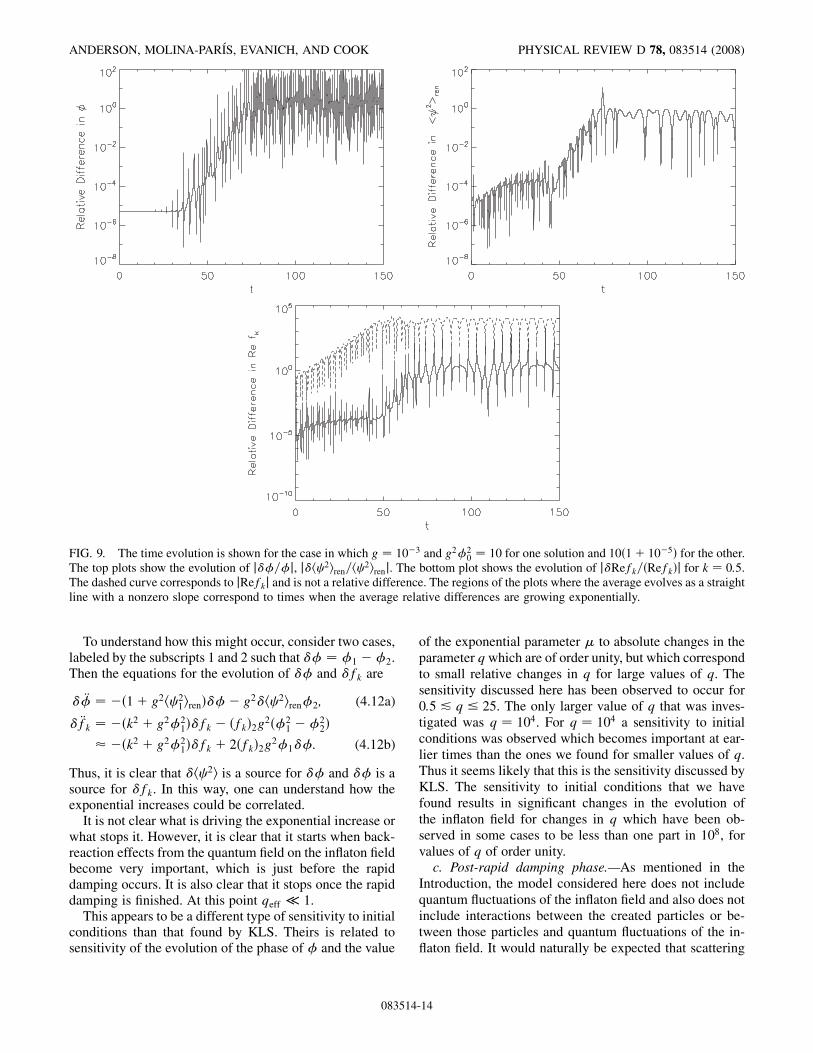
It is during this period, begun by the first rapid dampingof the inflaton field and finished by the second, that theextreme sensitivity to initial conditions that we have foundseems to manifest. A useful way to study the sensitivity isto look at the time evolution of the quantities �, g2h 2iren,and fk for two cases in which the initial data are almost butnot quite identical. For the cases discussed here, �0 isdifferent by a small amount, which then generates smallchanges in the initial values of the modes fk and thus ing2h 2iren. If the relative differences in the quantities

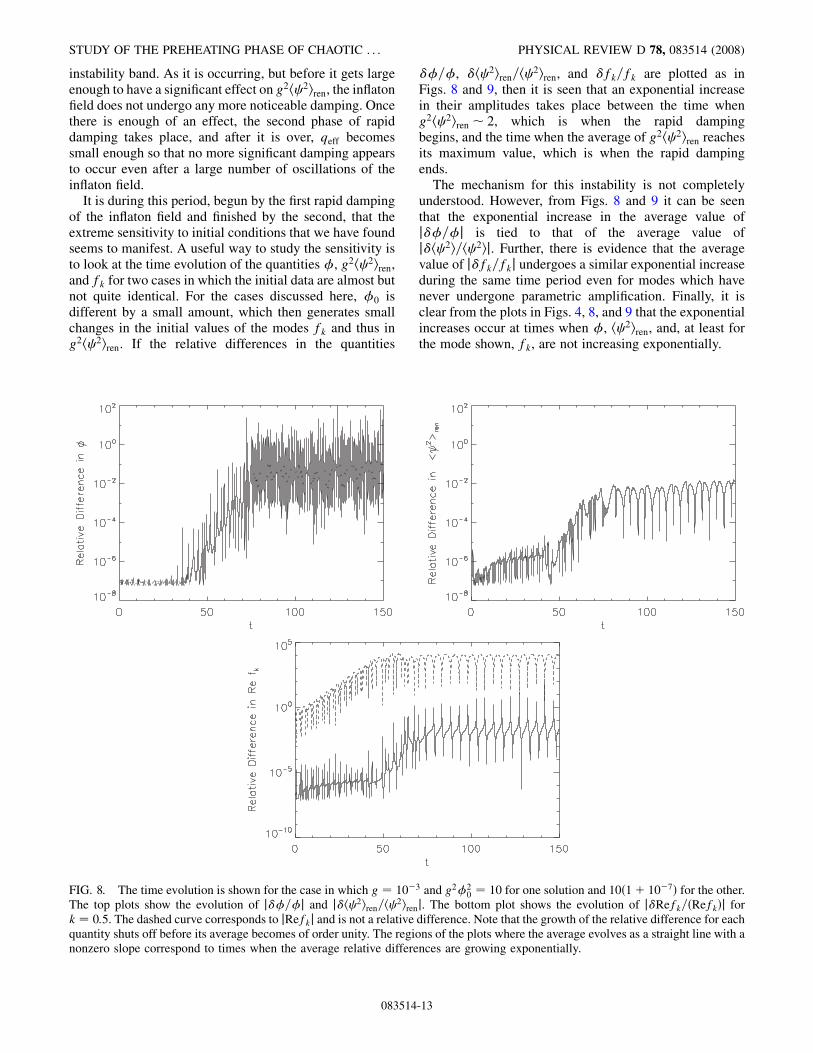
�=�, h 2iren=h 2iren, and fk=fk are plotted as inFigs. 8 and 9, then it is seen that an exponential increasein their amplitudes takes place between the time wheng2h 2iren 2, which is when the rapid dampingbegins, and the time when the average of g2h 2iren reachesits maximum value, which is when the rapid dampingends.The mechanism for this instability is not completely

understood. However, from Figs. 8 and 9 it can be seenthat the exponential increase in the average value ofj�=�j is tied to that of the average value ofjh 2i=h 2ij. Further, there is evidence that the averagevalue of jfk=fkj undergoes a similar exponential increaseduring the same time period even for modes which havenever undergone parametric amplification. Finally, it isclear from the plots in Figs. 4, 8, and 9 that the exponentialincreases occur at times when �, h 2iren, and, at least forthe mode shown, fk, are not increasing exponentially.

FIG. 8. The time evolution is shown for the case in which g ¼ 10�3 and g2�20 ¼ 10 for one solution and 10ð1þ 10�7Þ for the other.

The top plots show the evolution of j�=�j and jh 2iren=h 2irenj. The bottom plot shows the evolution of jRefk=ðRefkÞj fork ¼ 0:5. The dashed curve corresponds to jRefkj and is not a relative difference. Note that the growth of the relative difference for eachquantity shuts off before its average becomes of order unity. The regions of the plots where the average evolves as a straight line with anonzero slope correspond to times when the average relative differences are growing exponentially.


083514-13

To understand how this might occur, consider two cases,labeled by the subscripts 1 and 2 such that � ¼ �1 ��2.Then the equations for the evolution of � and fk are

€� ¼ �ð1þ g2h 21irenÞ�� g2h 2iren�2; (4.12a)

€fk ¼ �ðk2 þ g2�21Þfk � ðfkÞ2g2ð�2

1 ��22Þ

� �ðk2 þ g2�21Þfk þ 2ðfkÞ2g2�1�: (4.12b)

Thus, it is clear that h 2i is a source for � and � is asource for fk. In this way, one can understand how theexponential increases could be correlated.

It is not clear what is driving the exponential increase orwhat stops it. However, it is clear that it starts when back-reaction effects from the quantum field on the inflaton fieldbecome very important, which is just before the rapiddamping occurs. It is also clear that it stops once the rapiddamping is finished. At this point qeff � 1.

This appears to be a different type of sensitivity to initialconditions than that found by KLS. Theirs is related tosensitivity of the evolution of the phase of � and the value

of the exponential parameter � to absolute changes in theparameter qwhich are of order unity, but which correspondto small relative changes in q for large values of q. Thesensitivity discussed here has been observed to occur for0:5 & q � 25. The only larger value of q that was inves-tigated was q ¼ 104. For q ¼ 104 a sensitivity to initialconditions was observed which becomes important at ear-lier times than the ones we found for smaller values of q.Thus it seems likely that this is the sensitivity discussed byKLS. The sensitivity to initial conditions that we havefound results in significant changes in the evolution ofthe inflaton field for changes in q which have been ob-served in some cases to be less than one part in 108, forvalues of q of order unity.c. Post-rapid damping phase.—As mentioned in the

Introduction, the model considered here does not includequantum fluctuations of the inflaton field and also does notinclude interactions between the created particles or be-tween those particles and quantum fluctuations of the in-flaton field. It would naturally be expected that scattering

FIG. 9. The time evolution is shown for the case in which g ¼ 10�3 and g2�20 ¼ 10 for one solution and 10ð1þ 10�5Þ for the other.

The top plots show the evolution of j�=�j, jh 2iren=h 2irenj. The bottom plot shows the evolution of jRefk=ðRefkÞj for k ¼ 0:5.The dashed curve corresponds to jRefkj and is not a relative difference. The regions of the plots where the average evolves as a straightline with a nonzero slope correspond to times when the average relative differences are growing exponentially.


083514-14

due to these interactions would become important at somepoint and that they would lead to the thermalization of theparticles. Various studies which have taken such interac-tions into account [21,22,26,27,35] indicate that scatteringeffects will become important at intermediate times. Insome cases this may occur before the rapid damping phasehas ended [22,27]. Once the scattering becomes importantthe evolution should change significantly from that foundusing our model.

Nevertheless, it is of some interest to see what happensin our model at late times because of the insight it givesinto the effects of particle production in the context of thesemiclassical approximation. First, since quantum fluctua-tions of the inflaton field are ignored, one would expect thatthe damping of the inflaton field is due to the production ofparticles of the quantum fields. However, in the semiclas-sical approximation when the classical field is rapidlyvarying, different definitions of particle number can givedifferent answers [52]. Even if one has a good definition,the particles may not behave like ordinary particles. This isthe case here, as can be seen in the right-hand plot of Fig. 3.Recall that in Minkowski spacetime the total energy den-sity is conserved. Then it is clear from the plot that, afterthe rapid damping phase, most of the energy is transferredback and forth between the inflaton field and the quantumfield. Thus, the created particles have an energy densitythat is very different from what they would have if theinflaton field was slowly varying.

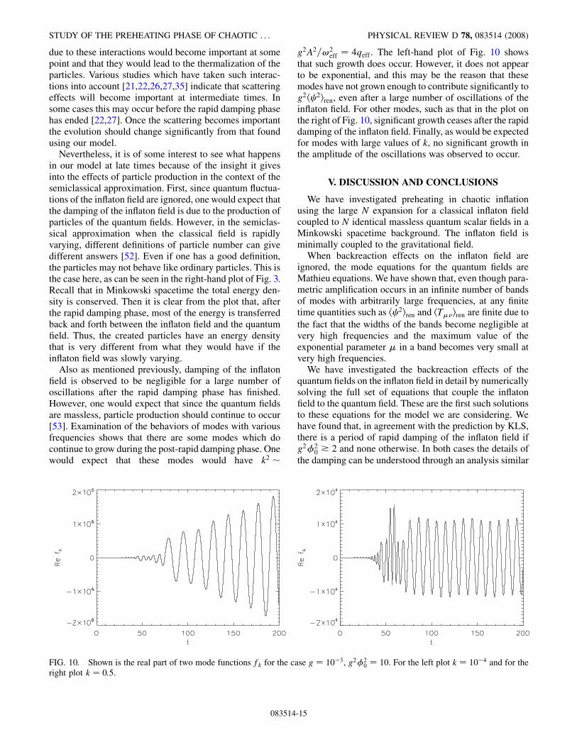
Also as mentioned previously, damping of the inflatonfield is observed to be negligible for a large number ofoscillations after the rapid damping phase has finished.However, one would expect that since the quantum fieldsare massless, particle production should continue to occur[53]. Examination of the behaviors of modes with variousfrequencies shows that there are some modes which docontinue to grow during the post-rapid damping phase. Onewould expect that these modes would have k2

g2A2=!2eff ¼ 4qeff . The left-hand plot of Fig. 10 shows

that such growth does occur. However, it does not appearto be exponential, and this may be the reason that thesemodes have not grown enough to contribute significantly tog2h 2iren, even after a large number of oscillations of theinflaton field. For other modes, such as that in the plot onthe right of Fig. 10, significant growth ceases after the rapiddamping of the inflaton field. Finally, as would be expectedfor modes with large values of k, no significant growth inthe amplitude of the oscillations was observed to occur.

V. DISCUSSION AND CONCLUSIONS

We have investigated preheating in chaotic inflationusing the large N expansion for a classical inflaton fieldcoupled to N identical massless quantum scalar fields in aMinkowski spacetime background. The inflaton field isminimally coupled to the gravitational field.When backreaction effects on the inflaton field are

ignored, the mode equations for the quantum fields areMathieu equations. We have shown that, even though para-metric amplification occurs in an infinite number of bandsof modes with arbitrarily large frequencies, at any finitetime quantities such as h 2iren and hT��iren are finite due tothe fact that the widths of the bands become negligible atvery high frequencies and the maximum value of theexponential parameter � in a band becomes very small atvery high frequencies.We have investigated the backreaction effects of the

quantum fields on the inflaton field in detail by numericallysolving the full set of equations that couple the inflatonfield to the quantum field. These are the first such solutionsto these equations for the model we are considering. Wehave found that, in agreement with the prediction by KLS,there is a period of rapid damping of the inflaton field ifg2�2

0 * 2 and none otherwise. In both cases the details of

the damping can be understood through an analysis similar

FIG. 10. Shown is the real part of two mode functions fk for the case g ¼ 10�3, g2�20 ¼ 10. For the left plot k ¼ 10�4 and for the

right plot k ¼ 0:5.


083514-15

to that done by KLS; this analysis involves studying theway in which the instability bands change as the inflatonfield damps. For g2�2

0 * 2 the situation depends upon the

locations of the instability bands, and therefore, there aredifferent ways in which the damping proceeds. For g2�2

0 &1 there is a brief period in which the amplitude of theinflaton field is rapidly damped but only by a very smallamount. This is followed by a long period of slow damp-ing. Thus, we distinguish this from the cases in which theinflaton field is rapidly damped by a significant amount.

The analysis by KLS shows that significant differencesin the evolution occur for realistic values of the initialconditions and parameters when the expansion of the uni-verse is taken into account. However, in cases where rapiddamping of the inflaton field occurs, it is possible to neglectthis expansion during the rapid damping phase. We findthat during the rapid damping phase there is more dampingof the inflaton field than was predicted originally by KLS.We also find that the rapid damping occurs in two burstsseparated by a period of time which is generally longerthan the time it takes for each period of rapid damping tooccur. Finally, we find that there is an extreme sensitivity toinitial conditions which manifests in significant changes inthe evolution of the inflaton field and the modes of thequantum fields during the period of rapid damping. Thiscan occur for changes in the initial amplitude of the in-flaton field as small as, or even smaller than, one part in108. This sensitivity is not well understood. Since it occursfor values of g2�2

0 * 2, it would seem to be different than

the one discussed by KLS, which only occurs for largevalues of g2�2

0.

ACKNOWLEDGMENTS

P. R. A. would like to thank L. Ford and B. L. Hu forhelpful conversations. We would like to thank L. Kofman,I. Lawrie, A. Linde, and A.A. Starobinsky for helpfulcomments regarding the manuscript. P. R.A. and C.M.-P.would like to thank the T8 group at Los Alamos NationalLaboratory for hospitality. They would also like to thankthe organizers of the Peyresq 5 Meeting for hospitality.P. R.A. would like to thank the Racah Institute of Physicsat Hebrew University, the Gravitation Group at theUniversity of Maryland, and the Department ofTheoretical Physics at the Universidad de Valencia forhospitality. P. R. A. acknowledges the Einstein Center atHebrew University, the Forchheimer Foundation, and theSpanish Ministerio de Educacion y Ciencia for financialsupport. C.M.-P. would like to thank the Department ofTheoretical Physics at the Universidad de Valencia forhospitality and the Leverhulme Trust for support. Thisresearch has been partially supported by Grant No. PHY-0070981, No. PHY-0555617, and No. PHY-0556292 fromthe National Science Foundation. Some of the numericalcomputations were performed on the Wake Forest

University DEAC Cluster with support from an IBMSUR grant and the Wake Forest University ISDepartment. Computational results were supported bystorage hardware awarded to Wake Forest Universitythrough an IBM SUR grant.

APPENDIX: RENORMALIZATION ANDCONSERVATION OF THE ENERGY-MOMENTUM

TENSOR

In this appendix the renormalization and conservation ofthe energy-momentum tensor for the system we are con-sidering are discussed. As discussed in Sec. II, at leadingorder in a large N expansion, the system is equivalent to amassive classical scalar field coupled to a single masslessquantum field. That in turn is equivalent to the systemdiscussed in Ref. [47], if the scale factor aðtÞ is set equalto 1, the coupling of the inflaton field to the scalar curvatureis set to zero, the coupling constant � is set equal to 2g2, themass of the quantum field is set to zero, and the ��3=3!term in the equation of motion for the � field is dropped.Because of this, we will use several results from Ref. [47]in what follows.We start with the quantum field theory in terms of bare

parameters. The bare equations of motion for the homoge-neous classical inflaton field and the quantum field modesare given in Eqs. (2.3) and (2.5), and an expression for thequantity h 2iB is given in Eq. (2.11). It is assumed through-out that (i) the inflaton field is homogeneous and thusdepends only on the time t and that (ii) the quantum field is in a homogeneous and isotropic state so that h 2idepends only on time, and hT��i, when expressed in terms

of the usual Cartesian components, is diagonal and de-pends only on time.The total bare energy-momentum tensor of the system is

given by [47]

TB�� ¼ TC;B�� þ hT��iQ;B; (A1a)

TC;B�� ¼ @��@�� 1

2��

��@��@��m2B

2��

2;

(A1b)

hT��iQ;B ¼ ð1� 2�BÞh@� @� iþ

�2�B � 1

2

��

��h@� @� i� 2�Bh @�@� i þ 2�B��h h i

� g2B�2

2��h 2i: (A1c)

We first show that the total energy-momentum tensor iscovariantly conserved. Since it is diagonal and dependsonly on time, the conservation equation in Minkowskispacetime is trivially satisfied for all of the componentsof TB��, except for T

Btt . This component has the explicit

form


083514-16

TC;Btt ¼ 1

2_�2 þm2

B

2�2; (A2a)

hTttiQ;B ¼ 1

4�2

Z þ1

0dkk2½j _fkj2 þ ðk2 þ g2B�

2Þjfkj2�:(A2b)

The conservation condition is

@tTBtt ¼ 0: (A3)

It is easy to show, making use of the equations of motionfor �ðtÞ and fkðtÞ, that

@tTC;Btt ¼ �g2B� _�h 2iB; (A4a)

@thTttiQ;B ¼ g2B�_�h 2iB; (A4b)

with h 2iB given by Eq. (2.11). This implies that the totalbare energy-momentum tensor is covariantly conserved.

Renormalization is accomplished through the method ofadiabatic regularization [40–43]. The details are given inRef. [47]. The result for h 2iB is

h 2iren ¼ h 2iB � h 2iad¼ 1

2�2

Z �

0dkk2

�jfkðtÞj2 � 1

2k

�

þ 1

2�2

Z þ1

�dkk2

�jfkðtÞj2 � 1

2kþ g2R�

2

4k3

�þ h 2ian; (A5a)

h 2ian ¼ � g2�2

8�2

�1� log

�2�

M

��: (A5b)

For the energy-momentum tensor

hTttiren ¼ TCtt þ hTttiQren ¼ TCtt þ hTttiQB � hTttiQad; (A6a)

with

TCtt ¼ 1

2_�2 þm2

2�2; (A6b)

hTttiQren ¼ 1

4�2

Z þ1

0dkk2½j _fkj2 þ ðk2 þ g2�2Þjfkj2�

� 1

4�2

Z �

0dkk2

�kþ g2�2

2k

�� 1

4�2

Z þ1

�dkk2

�kþ g2�2

2k� g4�4

8k3

�þ hTttiQan;

(A6c)

hTttiQan ¼ �g4�4

32�2

�1� log

�2"

M

��: (A6d)

We note that in Minkowski spacetime the bare and theadiabatic energy density of the quantum field do not de-pend on the value of the coupling � of the quantum field tothe scalar curvature. Thus, the renormalized value of theenergy density does not depend on �.Using Eqs. (A5) and (A6), and the equations of motion

for � and fk, it is easy to derive the following identities:

@tTCtt ¼ �g2� _�h 2iren; (A7a)

@thTttiQB ¼ g2� _�h 2iB; (A7b)

@thTttiQad ¼ g2� _�h 2iad: (A7c)

They can be used to show that

@thTttiren ¼ @thTttiC þ @thTttiQB � @thTttiQad¼ g2� _�½�h 2iren þ h 2iB � h 2iad� ¼ 0:

(A8)

[1] A. Linde, Lect. Notes Phys. 738, 1 (2008); R. H.Brandenberger, arXiv:hep-ph/0101119.

[2] E.W. Kolb, A.D. Linde, and A. Riotto, Phys. Rev. Lett.77, 4290 (1996).

[3] A. D. Dolgov and A.D. Linde, Phys. Lett. 116B, 329(1982); L. F. Abbott, E. Farhi, and M.B. Wise, Phys.Lett. 117B, 29 (1982).

[4] L. A. Kofman, arXiv:astro-ph/9605155.[5] A. Linde, Phys. Lett. 108B, 389 (1982); 114B, 431 (1982);

116B, 340 (1982); 116B, 335 (1982); A. Albrecht and P. J.Steinhardt, Phys. Rev. Lett. 48, 1220 (1982).

[6] A. D. Linde, Particle Physics and Inflationary Cosmology(Harwood, Chur, Switzerland, 1990).

[7] E.W. Kolb and M. S. Turner, The Early Universe(Addison-Wesley, Redwood, CA, 1990), Chap. 8.

[8] J. H. Traschen and R.H. Brandenberger, Phys. Rev. D 42,2491 (1990).

[9] L. F. Abbott, E. Farhi, and M. B. Wise, Phys. Lett. 117B,29 (1982); A. Albrecht, P. J. Steinhardt, M. S. Turner, andF. Wilczek, Phys. Rev. Lett. 48, 1437 (1982); A. D.Dolgov and A.D. Linde, Phys. Lett. 116B, 329 (1982);A. D. Dolgov and D. P. Kirilova, Yad. Fiz. 51, 273 (1990)[Sov. J. Nucl. Phys. 51, 172 (1990)].

[10] L. A. Kofman, A.D. Linde, and A.A. Starobinsky, Phys.Rev. Lett. 73, 3195 (1994).

[11] L. A. Kofman, A.D. Linde, and A.A. Starobinsky, Phys.Rev. Lett. 76, 1011 (1996).

[12] A. Dolgov and K. Freese, Phys. Rev. D 51, 2693 (1995); Y.Shtanov, J. H. Traschen, and R.H. Brandenberger, Phys.Rev. D 51, 5438 (1995); R. Allahverdi and B.A.Campbell, Phys. Lett. B 395, 169 (1997).

[13] D. Boyanovsky, H. J. de Vega, R. Holman, D. S. Lee, andA. Singh, Phys. Rev. D 51, 4419 (1995).

[14] See, for example, S. A. Ramsey and B. L. Hu, Phys. Rev. D


083514-17

56, 661 (1997), and references therein.[15] L. Kofman, A. Linde, and A.A. Starobinsky, Phys. Rev. D

56, 3258 (1997).[16] D. Boyanovsky and H. J. de Vega, Phys. Rev. D 47, 2343

(1993); D. Boyanovsky, M. D’Attanasio, H. J. de Vega, R.Holman, and D. S. Lee, String Gravity and Physics at thePlanck Energy Scale, Vol. 476, Proceedings of the NATOAdvanced Study Institute, Erice, Italy, 1995, edited byN.G. Sanchez and A. Zichichi (Kluwer AcademicPublishers, Dordrecht; Boston, 1996).

[17] D. Boyanovsky, M. D’Attanasio, H. J. de Vega, R.Holman, D. S. Lee, and A. Singh, arXiv:hep-ph/9505220.

[18] D. Boyanovsky, R. Holman, and S. P. Kumar, Phys. Rev. D56, 1958 (1997).

[19] D. Boyanovsky, M. D’Attanasio, H. J. de Vega, R.Holman, and D. S. Lee, Phys. Rev. D 52, 6805 (1995).

[20] F. Finelli and R. Brandenberger, Phys. Rev. Lett. 82, 1362(1999).

[21] S. Y. Khlebnikov and I. I. Tkachev, Phys. Rev. Lett. 77,219 (1996); arXiv:hep-ph/9603378; I. Tkachev, S.Khlebnikov, L. Kofman, and A.D. Linde, Phys. Lett. B440, 262 (1998).

[22] T. Prokopec and T.G. Roos, Phys. Rev. D 55, 3768(1997).

[23] G. N. Felder and L. Kofman, Phys. Rev. D 63, 103503(2001).

[24] S. Y. Khlebnikov and I. I. Tkachev, Phys. Rev. Lett. 79,1607 (1997).

[25] M. Desroche, G.N. Felder, J.M. Kratochvil, and A. Linde,Phys. Rev. D 71, 103516 (2005).

[26] D. I. Podolsky, G. N. Felder, L. Kofman, and M. PelosoPhys. Rev. D 73, 023501 (2006).

[27] J. F. Dufaux, G.N. Felder, L. Kofman, M. Peloso, and D.Podolsky, J. Cosmol. Astropart. Phys. 07 (2006) 006.

[28] G. N. Felder and L. Kofman, Phys. Rev. D 75, 043518(2007).

[29] G. N. Felder and I. I. Tkachev, Comput. Phys. Commun.178, 929 (2008).

[30] A. Chambers and A. Rajantie, Phys. Rev. Lett. 100,041302 (2008).

[31] D. Boyanovsky, H. J. de Vega, R. Holman, and J. F. J.Salgado, Phys. Rev. D 54, 7570 (1996).

[32] D. Boyanovsky, D. Cormier, H. J. de Vega, R. Holman, A.Singh, and M. Srednicki, Phys. Rev. D 56, 1939 (1997).

[33] S. A. Ramsey and B. L. Hu, Phys. Rev. D 56, 678(1997).

[34] J. Baacke, K. Heitmann, and C. Patzold, Phys. Rev. D 55,7815 (1997).

[35] J. Berges and J. Serreau, Phys. Rev. Lett. 91, 111601(2003).

[36] Y. Jin and S. Tsujikawa, Classical Quantum Gravity 23,353 (2006).

[37] D. N. Spergel et al. (WMAP), Astrophys. J. Suppl. Ser.170, 377 (2007); J. Lesgourgues and W. Valkenburg, Phys.Rev. D 75, 123519 (2007); J. Lesgourgues, A. A.Starobinsky, and W. Valkenburg, J. Cosmol. Astropart.Phys. 01 (2008) 010.

[38] F. Cooper, S. Habib, Y. Kluger, E. Mottola, J. P. Paz, andP. R. Anderson, Phys. Rev. D 50, 2848 (1994).

[39] K. c. Chou, Z. b. Su, B. l. Hao, and L. Yu, Phys. Rep. 118,1 (1985); R.D. Jordan, Phys. Rev. D 33, 444 (1986); E.Calzetta and B. L. Hu, Phys. Rev. D 35, 495 (1987).

[40] L. Parker, Ph.D. thesis, Harvard University, 1966 (XeroxUniversity Microfilms, Ann Arbor, Michigan, No. 73-31244), pp. 140–171 and App. CI.

[41] Ya. B. Zel’dovich and A.A. Starobinsky, Zh. Eksp. Teor.Fiz. 61, 2161 (1971) [Sov. Phys. JETP 34, 1159 (1971)].

[42] L. Parker and S.A. Fulling, Phys. Rev. D 9, 341 (1974);S. A. Fulling and L. Parker, Ann. Phys. (N.Y.) 87, 176(1974); S. A. Fulling, L. Parker, and B.-L. Hu, Phys. Rev.D 10, 3905 (1974).

[43] T. S. Bunch, J. Phys. A 13, 1297 (1980).[44] N. D. Birrell, Proc. R. Soc. A 361, 513 (1978).[45] P. R. Anderson and L. Parker, Phys. Rev. D 36, 2963

(1987).[46] P. R. Anderson and W. Eaker, Phys. Rev. D 61, 024003

(1999).[47] C. Molina-Parıs, P. R. Anderson, and S. A. Ramsey, Phys.

Rev. D 61, 127501 (2000).[48] N.W. McLachlan, Theory and Application of Mathieu

Functions (Dover, New York, 1961).[49] J. Mathews and R. L. Walker, Mathematical Methods of

Physics (Addison-Wesley, London, 1973).[50] M. Abramowitz and I. A. Stegun, Handbook of

Mathematical Functions (Dover, New York, 1972).[51] David Evanich, Master thesis, Wake Forest University,

2006 (unpublished).[52] See, for example, N. D. Birrell and P. C.W. Davies,

Quantum Fields in Curved Space (Cambridge UniversityPress, Cambridge, England, 1982), and references con-tained therein.

[53] L. Ford (private communication).


083514-18

Documents

Studyof the preheating phase of chaotic inﬂation