Embed Size (px)
Citation preview

Basic Introduction to STELLAII
Dr. Richard Palmer
Professor of Civil and Environmental Engineering
Box 352700
University of Washington
Seattle, Washington 98195-2700
(206) 685-2658
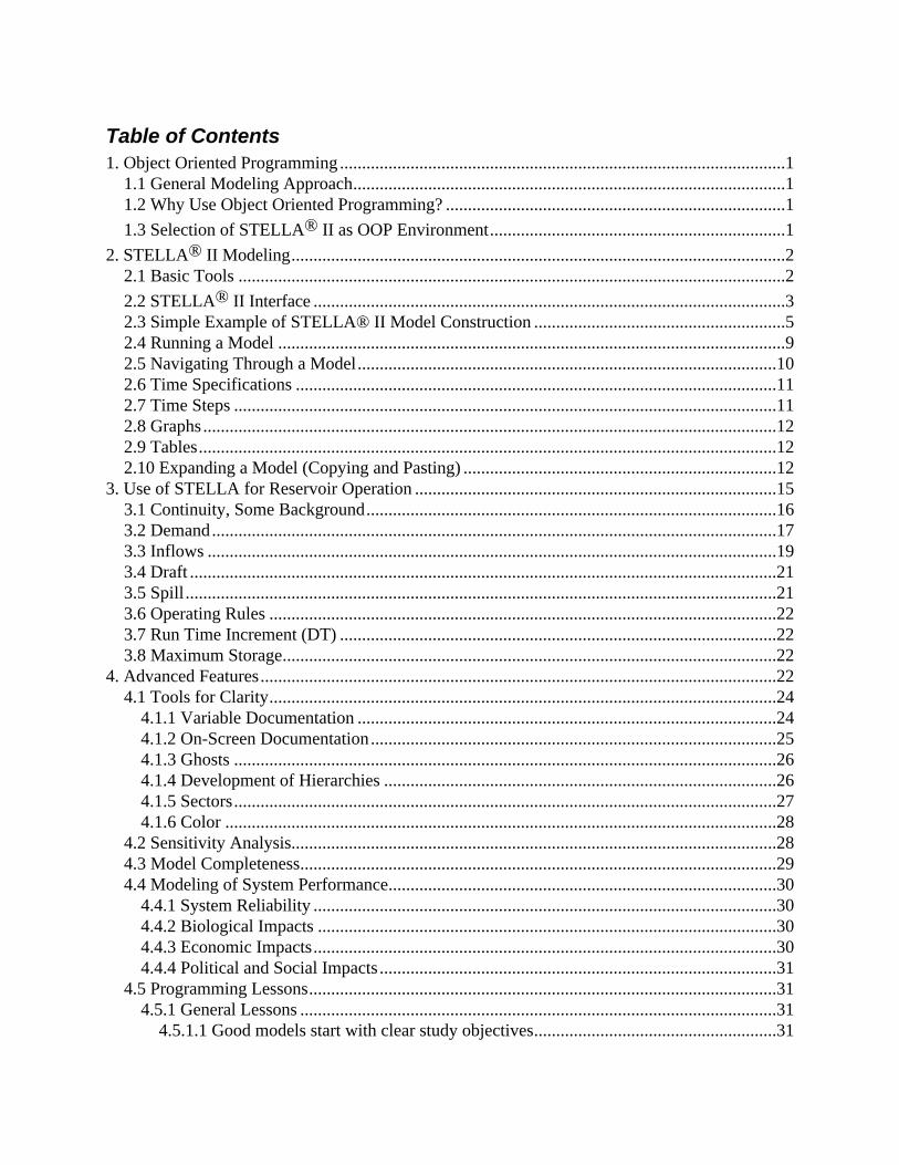
Table of Contents1. Object Oriented Programming .....................................................................................................1
1.1 General Modeling Approach..................................................................................................11.2 Why Use Object Oriented Programming? .............................................................................1
1.3 Selection of STELLA® II as OOP Environment...................................................................1
2. STELLA® II Modeling................................................................................................................22.1 Basic Tools ............................................................................................................................2
2.2 STELLA® II Interface ...........................................................................................................32.3 Simple Example of STELLA® II Model Construction .........................................................52.4 Running a Model ...................................................................................................................92.5 Navigating Through a Model...............................................................................................102.6 Time Specifications .............................................................................................................112.7 Time Steps ...........................................................................................................................112.8 Graphs..................................................................................................................................122.9 Tables...................................................................................................................................122.10 Expanding a Model (Copying and Pasting) .......................................................................12
3. Use of STELLA for Reservoir Operation ..................................................................................153.1 Continuity, Some Background.............................................................................................163.2 Demand................................................................................................................................173.3 Inflows .................................................................................................................................193.4 Draft .....................................................................................................................................213.5 Spill......................................................................................................................................213.6 Operating Rules ...................................................................................................................223.7 Run Time Increment (DT) ...................................................................................................223.8 Maximum Storage................................................................................................................22
4. Advanced Features.....................................................................................................................224.1 Tools for Clarity...................................................................................................................24
4.1.1 Variable Documentation ...............................................................................................244.1.2 On-Screen Documentation............................................................................................254.1.3 Ghosts ...........................................................................................................................264.1.4 Development of Hierarchies .........................................................................................264.1.5 Sectors...........................................................................................................................274.1.6 Color .............................................................................................................................28
4.2 Sensitivity Analysis..............................................................................................................284.3 Model Completeness............................................................................................................294.4 Modeling of System Performance........................................................................................30
4.4.1 System Reliability .........................................................................................................304.4.2 Biological Impacts ........................................................................................................304.4.3 Economic Impacts.........................................................................................................304.4.4 Political and Social Impacts ..........................................................................................31
4.5 Programming Lessons..........................................................................................................314.5.1 General Lessons ............................................................................................................31
4.5.1.1 Good models start with clear study objectives.......................................................31
4.5.1.2 Good models continue with a definition of what is important in the system.........324.5.1.3 Time allocation during modeling effort .................................................................324.5.1.4 Model Clarity .........................................................................................................324.5.1.5 Simplicity vs. Complexity......................................................................................32
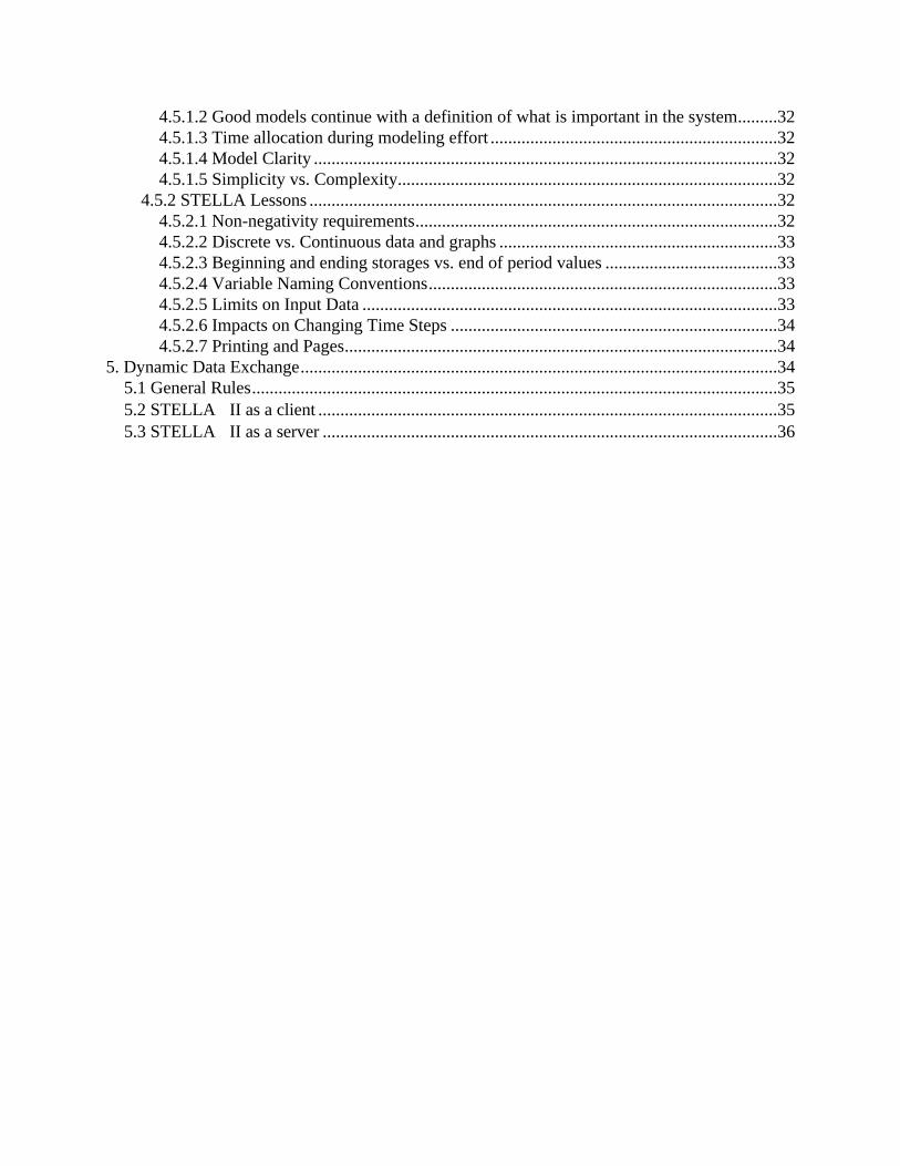
4.5.2 STELLA Lessons ..........................................................................................................324.5.2.1 Non-negativity requirements..................................................................................324.5.2.2 Discrete vs. Continuous data and graphs ...............................................................334.5.2.3 Beginning and ending storages vs. end of period values .......................................334.5.2.4 Variable Naming Conventions...............................................................................334.5.2.5 Limits on Input Data ..............................................................................................334.5.2.6 Impacts on Changing Time Steps ..........................................................................344.5.2.7 Printing and Pages..................................................................................................34
5. Dynamic Data Exchange............................................................................................................345.1 General Rules.......................................................................................................................355.2 STELLAII as a client ........................................................................................................355.3 STELLAII as a server .......................................................................................................36
List of FiguresFIGURE 2.1. BASIC MODELING ICONS IN STELLA ............................................................................................3FIGURE 2.2. BASIC STELLA USER INTERFACE...................................................................................................4FIGURE 2.3. COMPONENTS OF CHECKING ACCOUNT EXAMPLE..................................................................5FIGURE 2.4. LINKING THE COMPONENTS OF CHECKING ACCOUNT EXAMPLE .......................................6FIGURE 2.5. DEVELOPING CAUSAL RELATIONSHIPS IN THE CHECKING ACCOUNT
EXAMPLE...........................................................................................................................................................7FIGURE 2.6. ENTERING VALUE FOR INCOME INTO THE CHECKING ACCOUNT EXAMPLE....................8FIGURE 2.7. ENTERING FUNCTIONAL RELATIONSHIP FOR ACCOUNT_TRANSFER INTO THE
CHECKING ACCOUNT EXAMPLE .................................................................................................................9FIGURE 2.8. MAIN MENU IN A STELLA MODEL.................................................................................................9FIGURE 2.9. OPTIONS FOR RUNNING A MODEL ..............................................................................................10FIGURE 2.10. OPTIONS FOR TIME SPECIFICATIONS .......................................................................................11FIGURE 2.11. OPTIONS FOR GRAPH FUNCTION...............................................................................................12FIGURE 2.12. COPYING THE ICONS OF A STELLA DIAGRAM .......................................................................13FIGURE 2.13. RESULT AFTER COPYING AND PASTING ICONS.....................................................................15FIGURE 3.1. COMPONENTS OF SIMPLE RESERVOIR MODEL........................................................................16FIGURE 3.2. DEVELOPING DEMAND ..................................................................................................................17FIGURE 3.3. DEVELOPING DEMAND ..................................................................................................................18FIGURE 3.4. DEFINING THE CONVERTER MGD\ACT\MONTH.......................................................................19FIGURE 3.5. MAKING DATA A FUNCTION OF TIME........................................................................................20FIGURE 3.6. PREPARING DATA CONVERTER FOR INPUT..............................................................................20FIGURE 3.7. INPUT OF VALUES TO ICON DATA...............................................................................................21FIGURE 4.1. WELL-CONSTRUCTED STELLA MODEL OF A SIMPLE RESERVOIR SYSTEM .....................23FIGURE 4.2. POORLY CONSTRUCTED STELLA MODEL OF A SIMPLE RESERVOIR SYSTEM.................24FIGURE 4.3. VARIABLE DOCUMENTATION IN STELLA MODEL ..................................................................25FIGURE 4.4. ON-SCREEN DOCUMENTATION IN STELLA MODEL................................................................26FIGURE 4.5. SECTOR IN STELLA MODEL...........................................................................................................28FIGURE 4.6. SENSITIVITY SPECIFICATIONS IN STELLA MODEL .................................................................29
1. Object Oriented ProgrammingThe modeling approach taken in this project is significantly different from that typicallytaken in the development of water resources planning and management models.Specifically, the major players in the management of water resources in the region wereidentified, interviewed to determine what should be in the model and then encouraged tobe actively involved in the model construction. This involvement was achieved with theuse of workshops and further interviews.
1.1 General Modeling ApproachTo allow for the participation of non-programmers in the modeling process, an object-oriented programming environment was selected. This environment provides a graphical,object-oriented interface that allows the user to model complex systems without requiringproficiency in computer programming. An understanding of important systemcomponents and their interactions are the primary prerequisites for model development.Thus, the start up time for model development in these environments is minimal.
The developer interface for object-oriented models is very different than those fortraditional programming languages such as FORTRAN. Rather than writing instructionsline by line, the user builds a model using a set of object icons. Each object represents atype of action or process and has specific attributes that define how it interacts with otherobjects in the system. To create a model in this environment, the user selects appropriateicons to emulate important system components. Relations between objects are thenestablished by graphically drawing appropriate connections. Once these connections areestablished, the user specifies the functional relationships between components and initialvalues to complete the model. This user interface is more efficient than traditionalprogramming in terms of time required developing the model.
1.2 Why Use Object Oriented Programming?There are five primary advantages in using object-oriented programming (OOP) for theconstruction of water resources models. They are: 1) the increased speed of modeldevelopment, 2) the ease of model modification, 3) the facility with which model resultscan be communicated, 4) the possibility of group model development, and 5) the trustdeveloped in the model. Each of these advantages will become obvious as the descriptionof model development and implementation is described. We will return to theseadvantages in the summary section.
1.3 Selection of STELLA® II as OOP EnvironmentThe OOP environment chosen to develop the models of the WIRM Model of Bull RunWater Supply for the Portland Water Bureau was STELLA® II. This software isdeveloped and marketed by High Performance Systems. Throughout the remainder ofthis report the term STELLA refers to High Performance System's latest software release,
2
STELLA® II version 5.1.1. STELLA was first sold in 1986 and has been used inacademic, research and consulting environments since that time. It is arguably the mostpopular and efficient tool available for constructing graphical simulation models currentlyon the market. Product sales have continued to increase in recent years and it has begunreceiving significant attention from the professional water resource managementcommunity.
2. STELLA® II ModelingAs indicated previously, STELLA (Systems Thinking Environment) is an object-oriented,graphical modeling environment. In this environment a few basic icons (or objects)simulate processes. This chapter contains a description of the basic icons and a simplemodel. Basic features of the STELLA environment are then explored using this example.
2.1 Basic ToolsModel development using object-oriented programming (OOP), such as STELLA is bothsimilar to and different from typical model development. Like typical development, thefunctions the model performs must be defined, the system must be conceptualized and amodel constructed. The relationships of each component to one another must beestablished. In some cases, these relationships may be physical relationships. Forinstance, the storage behind a dam at a point in time is affected by the storage in theprevious period, the volume of inflow during the ensuing period, the releases and spillsmade from the dam, and the dam's capacity. In other cases, these relationships may bemore conceptual in nature.
However, the manner in which these components are incorporated into the programmingenvironment in OOP is remarkably different from more conventional languages such asFORTRAN. Using OOP, once a component is identified, it is incorporated into themodel by defining it as a unique object. In this fashion it is assigned a specific label orname.
It is difficult to illustrate the process of developing models in an OOP environmentwithout the aid of animation. Initial stages of model development are similar to usingcomputer drafting or drawing software in which the user simply selects from a series ofexisting icons or templates and draws what is desired. When initiating the modelingprocess, the model builder is presented with a blank page onto which all of thecomponents necessary to model the system are placed. There are four basic tools in theSTELLA environment for model diagram development: Stocks Flows, Converters andConnectors (Figure 2.1).
Stocks are used to represent system components that can accumulate material over time.Stocks can reflect the system state or condition as it changes over time. In the examplesthat follow, reservoirs are always represented as stocks. Stocks often represent otheritems as well. For instance, stocks define the cumulative differences between an in-
3
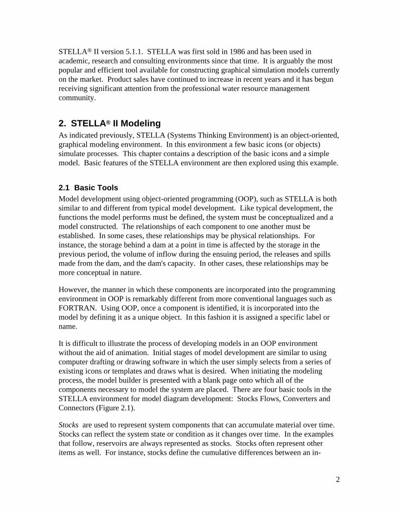
stream fish flow and a release. In STELLA, a rectangular icon represents stocks (asshown in Figure 2.1).
Figure 2.1. Basic Modeling Icons in STELLA
Flows represent components whose values are measured as rates. These rates may be aconstant, a function of time or a function of some other component in the system. A flowcan supply or drain a stock by flowing into or out of it. For example, inflows, spills andreleases from reservoirs are flows. The flow icon is the directed pipe with a flowregulator attached (see Figure 2.1). Flows can also be bi-directional, indicating that flowcan go in either direction.
Converters can represent constants, variables, functions, or time series. They also cantransform stocks and flows into other values. Converters can be represented as graphicalfunctions. This enables the modeler to sketch relationships between model variableswithout resorting to complex analytical expressions. A circular icon (Figure 2.1)represents convertors.
Connectors indicate the cause/effect relationship between diagram components. If aconnector is drawn from one component (circle end) to another (tip of the arrow) then thefirst component defines (or influences) the value of the second component. Thisgraphical indication of interaction helps model users understand STELLA diagrams.
The four basic building blocks of STELLA are described on pages 4-9 to 4-22 of theSTELLA Tutorial and Technical Documentation Manual.
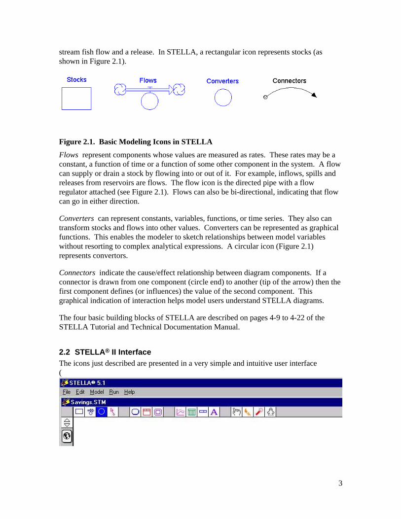
2.2 STELLA® II InterfaceThe icons just described are presented in a very simple and intuitive user interface(
4
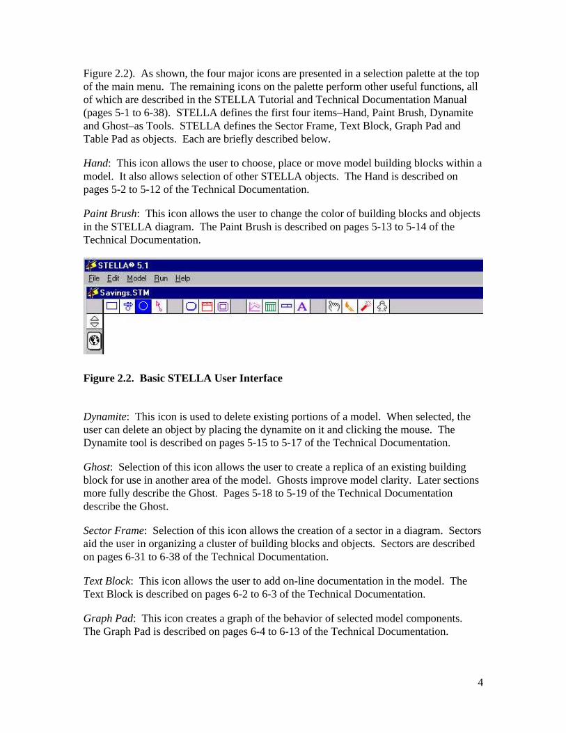
Figure 2.2). As shown, the four major icons are presented in a selection palette at the topof the main menu. The remaining icons on the palette perform other useful functions, allof which are described in the STELLA Tutorial and Technical Documentation Manual(pages 5-1 to 6-38). STELLA defines the first four items–Hand, Paint Brush, Dynamiteand Ghost–as Tools. STELLA defines the Sector Frame, Text Block, Graph Pad andTable Pad as objects. Each are briefly described below.
Hand: This icon allows the user to choose, place or move model building blocks within amodel. It also allows selection of other STELLA objects. The Hand is described onpages 5-2 to 5-12 of the Technical Documentation.
Paint Brush: This icon allows the user to change the color of building blocks and objectsin the STELLA diagram. The Paint Brush is described on pages 5-13 to 5-14 of theTechnical Documentation.
Figure 2.2. Basic STELLA User Interface
Dynamite: This icon is used to delete existing portions of a model. When selected, theuser can delete an object by placing the dynamite on it and clicking the mouse. TheDynamite tool is described on pages 5-15 to 5-17 of the Technical Documentation.
Ghost: Selection of this icon allows the user to create a replica of an existing buildingblock for use in another area of the model. Ghosts improve model clarity. Later sectionsmore fully describe the Ghost. Pages 5-18 to 5-19 of the Technical Documentationdescribe the Ghost.
Sector Frame: Selection of this icon allows the creation of a sector in a diagram. Sectorsaid the user in organizing a cluster of building blocks and objects. Sectors are describedon pages 6-31 to 6-38 of the Technical Documentation.
Text Block: This icon allows the user to add on-line documentation in the model. TheText Block is described on pages 6-2 to 6-3 of the Technical Documentation.
Graph Pad: This icon creates a graph of the behavior of selected model components.The Graph Pad is described on pages 6-4 to 6-13 of the Technical Documentation.
5
Table Pad: This icon creates a table of values over time for selected model components.The Table Pad is described on pages 6-14 to 6-28 of the Technical Documentation.
2.3 Simple Example of STELLA® II Model ConstructionA good example is a simple personal finance model.
Steve receives $3,000 a month in income. This amount is not expectedto change over the next year. His monthly expenses can be divided intotwo categories: fixed costs (rent, food, clothing, etc.) and variable costs.Fixed costs are also a constant value of $1,500. The variable costs are afunction of how rich Steve feels. Steve spends 25% of all the money hehas in his checking account over $2,000. Because he recognizes thistendency, he often transfers money between his checking account and hissavings account. Currently, he transfers all of the money greater than$3,000 from his checking account into his savings account.
There are four steps to take in creating a STELLA model
1. define variables in the problem and translate them into STELLA notation;2. link stocks and flows;3. define influences between stocks, flows, and converters;4. create functional relationships between stocks, flows, and converters.
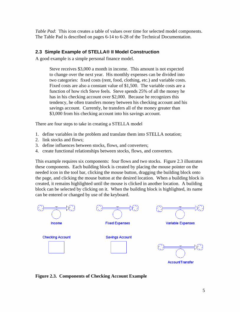
This example requires six components: four flows and two stocks. Figure 2.3 illustratesthese components. Each building block is created by placing the mouse pointer on theneeded icon in the tool bar, clicking the mouse button, dragging the building block ontothe page, and clicking the mouse button at the desired location. When a building block iscreated, it remains highlighted until the mouse is clicked in another location. A buildingblock can be selected by clicking on it. When the building block is highlighted, its namecan be entered or changed by use of the keyboard.
Figure 2.3. Components of Checking Account Example
6
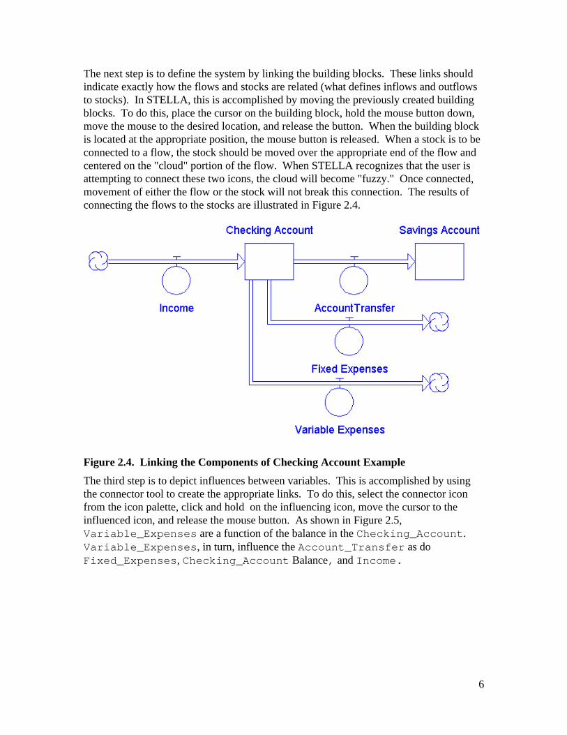
The next step is to define the system by linking the building blocks. These links shouldindicate exactly how the flows and stocks are related (what defines inflows and outflowsto stocks). In STELLA, this is accomplished by moving the previously created buildingblocks. To do this, place the cursor on the building block, hold the mouse button down,move the mouse to the desired location, and release the button. When the building blockis located at the appropriate position, the mouse button is released. When a stock is to beconnected to a flow, the stock should be moved over the appropriate end of the flow andcentered on the "cloud" portion of the flow. When STELLA recognizes that the user isattempting to connect these two icons, the cloud will become "fuzzy." Once connected,movement of either the flow or the stock will not break this connection. The results ofconnecting the flows to the stocks are illustrated in Figure 2.4.
Figure 2.4. Linking the Components of Checking Account Example
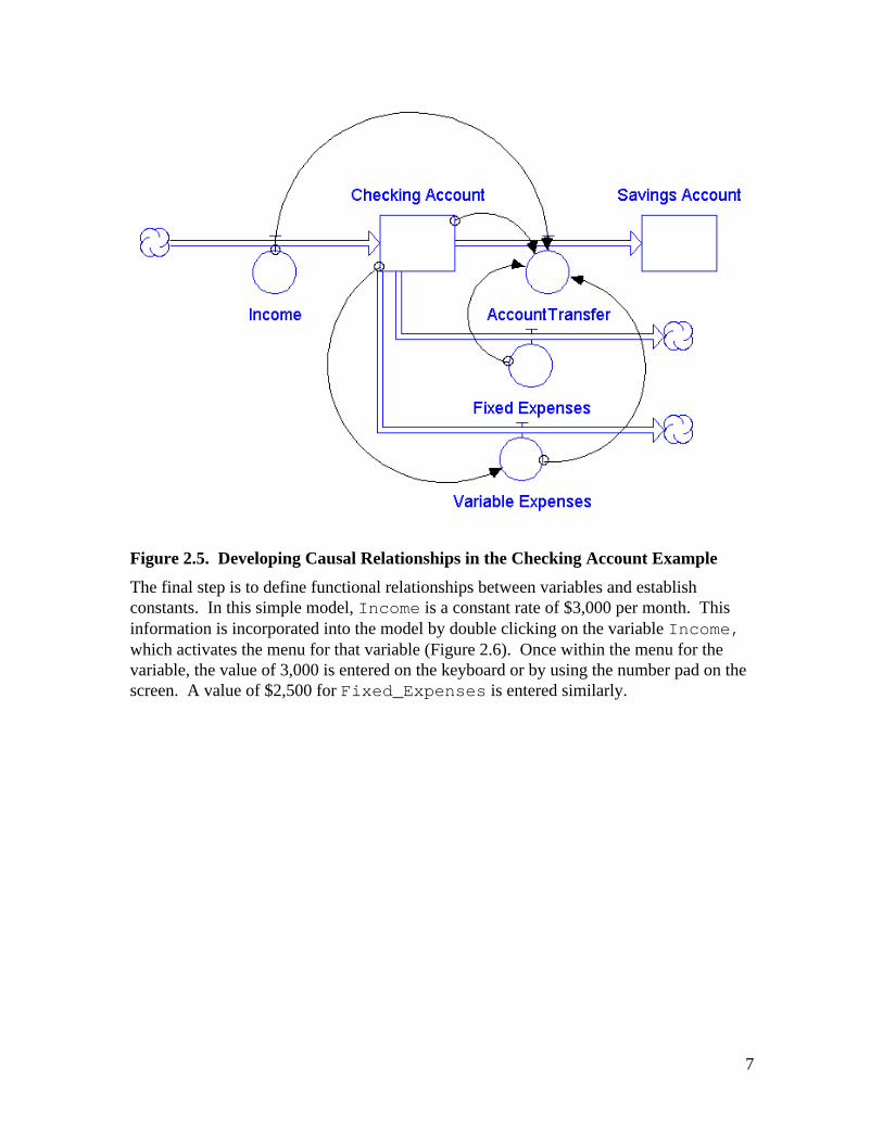
The third step is to depict influences between variables. This is accomplished by usingthe connector tool to create the appropriate links. To do this, select the connector iconfrom the icon palette, click and hold on the influencing icon, move the cursor to theinfluenced icon, and release the mouse button. As shown in Figure 2.5,Variable_Expenses are a function of the balance in the Checking_Account.Variable_Expenses, in turn, influence the Account_Transfer as doFixed_Expenses, Checking_Account Balance, and Income.
7
Figure 2.5. Developing Causal Relationships in the Checking Account Example
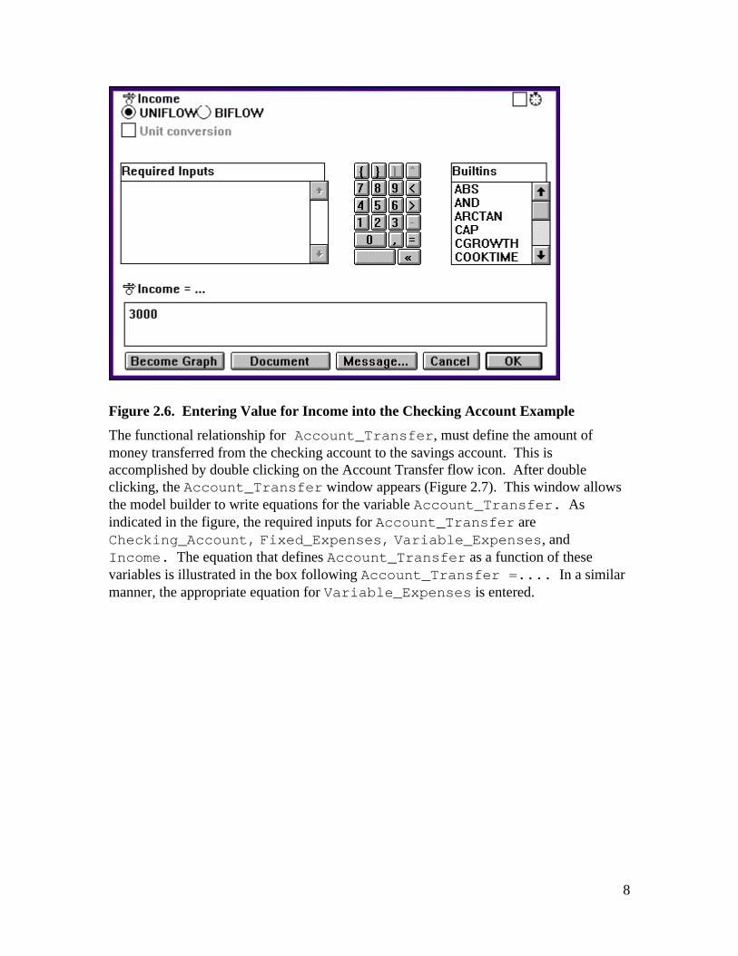
The final step is to define functional relationships between variables and establishconstants. In this simple model, Income is a constant rate of $3,000 per month. Thisinformation is incorporated into the model by double clicking on the variable Income,which activates the menu for that variable (Figure 2.6). Once within the menu for thevariable, the value of 3,000 is entered on the keyboard or by using the number pad on thescreen. A value of $2,500 for Fixed_Expenses is entered similarly.
8
Figure 2.6. Entering Value for Income into the Checking Account Example
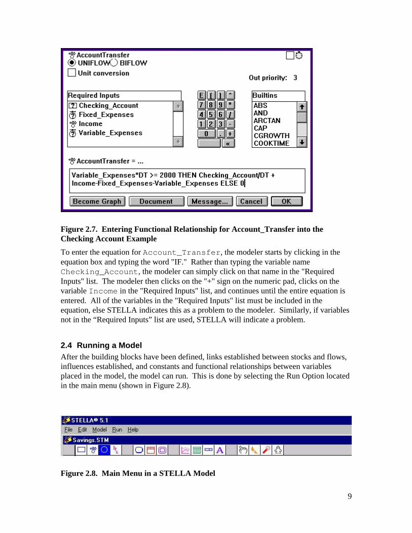
The functional relationship for Account_Transfer, must define the amount ofmoney transferred from the checking account to the savings account. This isaccomplished by double clicking on the Account Transfer flow icon. After doubleclicking, the Account_Transfer window appears (Figure 2.7). This window allowsthe model builder to write equations for the variable Account_Transfer. Asindicated in the figure, the required inputs for Account_Transfer areChecking_Account, Fixed_Expenses, Variable_Expenses, andIncome. The equation that defines Account_Transfer as a function of thesevariables is illustrated in the box following Account_Transfer =.... In a similarmanner, the appropriate equation for Variable_Expenses is entered.
9
Figure 2.7. Entering Functional Relationship for Account_Transfer into theChecking Account Example
To enter the equation for Account_Transfer, the modeler starts by clicking in theequation box and typing the word "IF." Rather than typing the variable nameChecking_Account, the modeler can simply click on that name in the "RequiredInputs" list. The modeler then clicks on the "+" sign on the numeric pad, clicks on thevariable Income in the "Required Inputs" list, and continues until the entire equation isentered. All of the variables in the "Required Inputs" list must be included in theequation, else STELLA indicates this as a problem to the modeler. Similarly, if variablesnot in the “Required Inputs” list are used, STELLA will indicate a problem.
2.4 Running a ModelAfter the building blocks have been defined, links established between stocks and flows,influences established, and constants and functional relationships between variablesplaced in the model, the model can run. This is done by selecting the Run Option locatedin the main menu (shown in Figure 2.8).
Figure 2.8. Main Menu in a STELLA Model
10
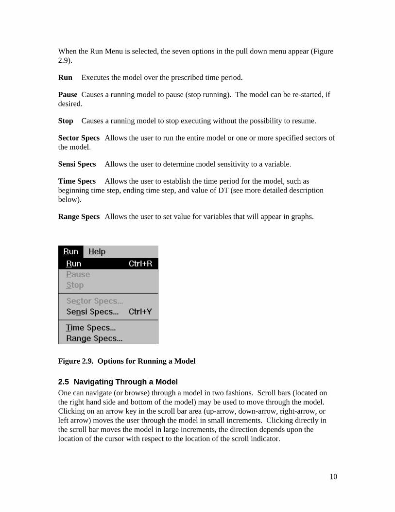
When the Run Menu is selected, the seven options in the pull down menu appear (Figure2.9).
Run Executes the model over the prescribed time period.
Pause Causes a running model to pause (stop running). The model can be re-started, ifdesired.
Stop Causes a running model to stop executing without the possibility to resume.
Sector Specs Allows the user to run the entire model or one or more specified sectors ofthe model.
Sensi Specs Allows the user to determine model sensitivity to a variable.
Time Specs Allows the user to establish the time period for the model, such asbeginning time step, ending time step, and value of DT (see more detailed descriptionbelow).
Range Specs Allows the user to set value for variables that will appear in graphs.
Figure 2.9. Options for Running a Model
2.5 Navigating Through a ModelOne can navigate (or browse) through a model in two fashions. Scroll bars (located onthe right hand side and bottom of the model) may be used to move through the model.Clicking on an arrow key in the scroll bar area (up-arrow, down-arrow, right-arrow, orleft arrow) moves the user through the model in small increments. Clicking directly inthe scroll bar moves the model in large increments, the direction depends upon thelocation of the cursor with respect to the location of the scroll indicator.
11
One may also "zoom" in and out of a diagram using the Zoom buttons located at thebottom left of the diagram and shown as "+" and "-" signs. For complex models,zooming out allows the modeler and model user to obtain an overview of all modelcomponents.
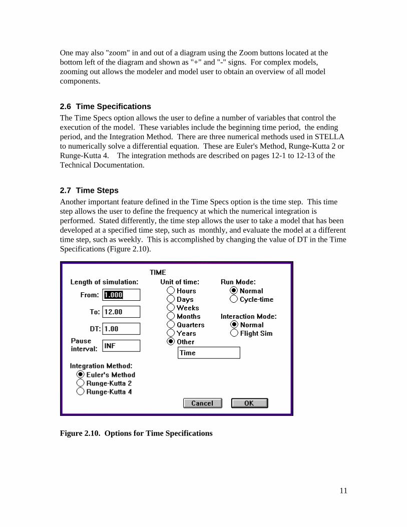
2.6 Time SpecificationsThe Time Specs option allows the user to define a number of variables that control theexecution of the model. These variables include the beginning time period, the endingperiod, and the Integration Method. There are three numerical methods used in STELLAto numerically solve a differential equation. These are Euler's Method, Runge-Kutta 2 orRunge-Kutta 4. The integration methods are described on pages 12-1 to 12-13 of theTechnical Documentation.
2.7 Time StepsAnother important feature defined in the Time Specs option is the time step. This timestep allows the user to define the frequency at which the numerical integration isperformed. Stated differently, the time step allows the user to take a model that has beendeveloped at a specified time step, such as monthly, and evaluate the model at a differenttime step, such as weekly. This is accomplished by changing the value of DT in the TimeSpecifications (Figure 2.10).
Figure 2.10. Options for Time Specifications
12
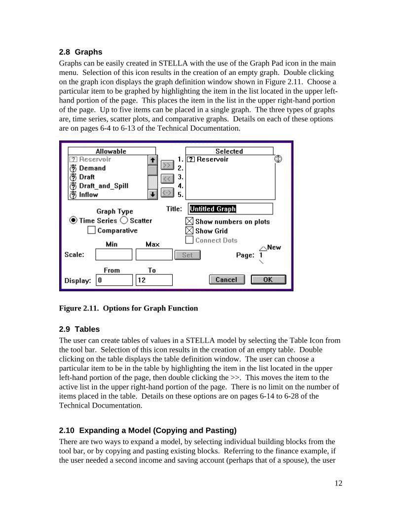
2.8 GraphsGraphs can be easily created in STELLA with the use of the Graph Pad icon in the mainmenu. Selection of this icon results in the creation of an empty graph. Double clickingon the graph icon displays the graph definition window shown in Figure 2.11. Choose aparticular item to be graphed by highlighting the item in the list located in the upper left-hand portion of the page. This places the item in the list in the upper right-hand portionof the page. Up to five items can be placed in a single graph. The three types of graphsare, time series, scatter plots, and comparative graphs. Details on each of these optionsare on pages 6-4 to 6-13 of the Technical Documentation.
Figure 2.11. Options for Graph Function
2.9 TablesThe user can create tables of values in a STELLA model by selecting the Table Icon fromthe tool bar. Selection of this icon results in the creation of an empty table. Doubleclicking on the table displays the table definition window. The user can choose aparticular item to be in the table by highlighting the item in the list located in the upperleft-hand portion of the page, then double clicking the >>. This moves the item to theactive list in the upper right-hand portion of the page. There is no limit on the number ofitems placed in the table. Details on these options are on pages 6-14 to 6-28 of theTechnical Documentation.
2.10 Expanding a Model (Copying and Pasting)There are two ways to expand a model, by selecting individual building blocks from thetool bar, or by copying and pasting existing blocks. Referring to the finance example, ifthe user needed a second income and saving account (perhaps that of a spouse), the user
13
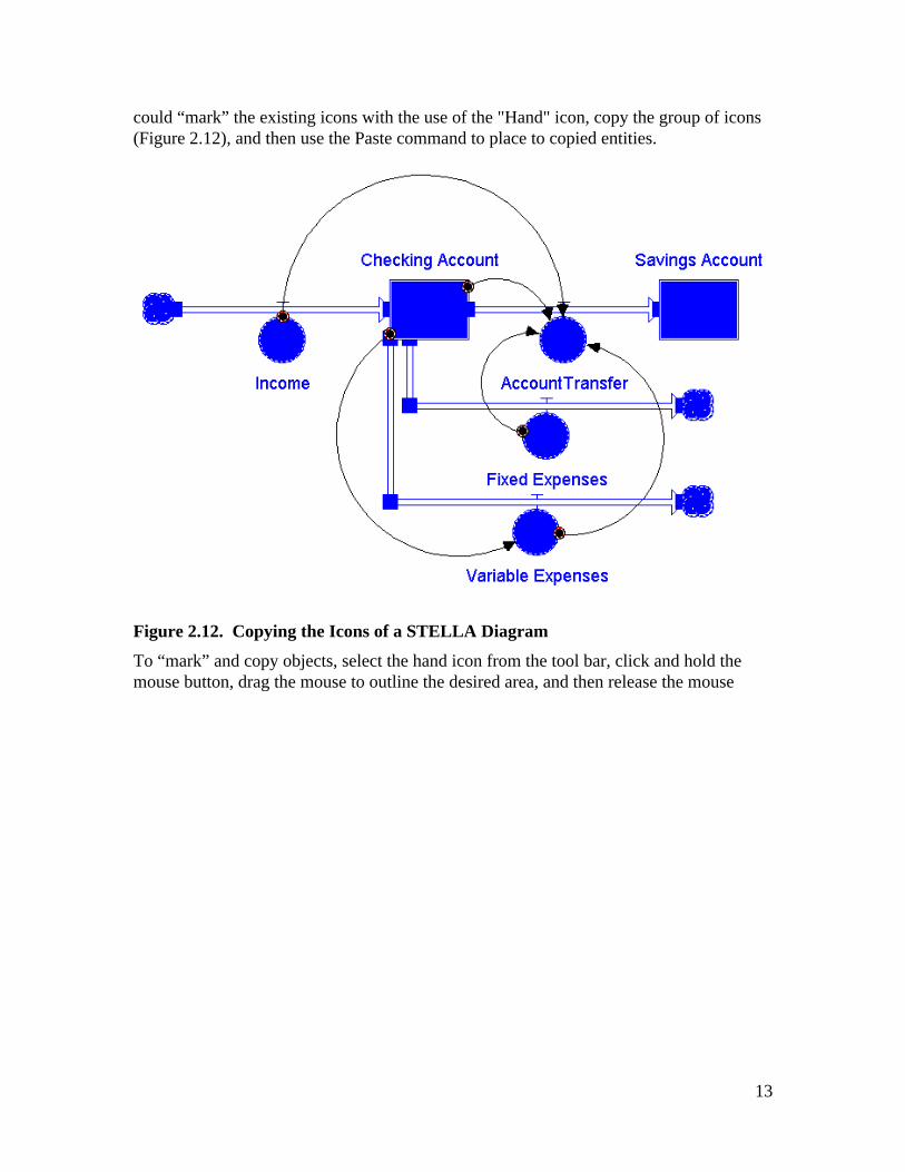
could “mark” the existing icons with the use of the "Hand" icon, copy the group of icons(Figure 2.12), and then use the Paste command to place to copied entities.
Figure 2.12. Copying the Icons of a STELLA Diagram
To “mark” and copy objects, select the hand icon from the tool bar, click and hold themouse button, drag the mouse to outline the desired area, and then release the mouse
14
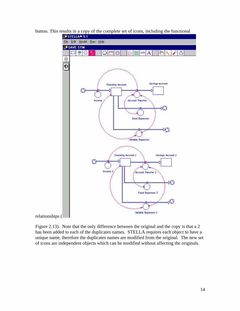
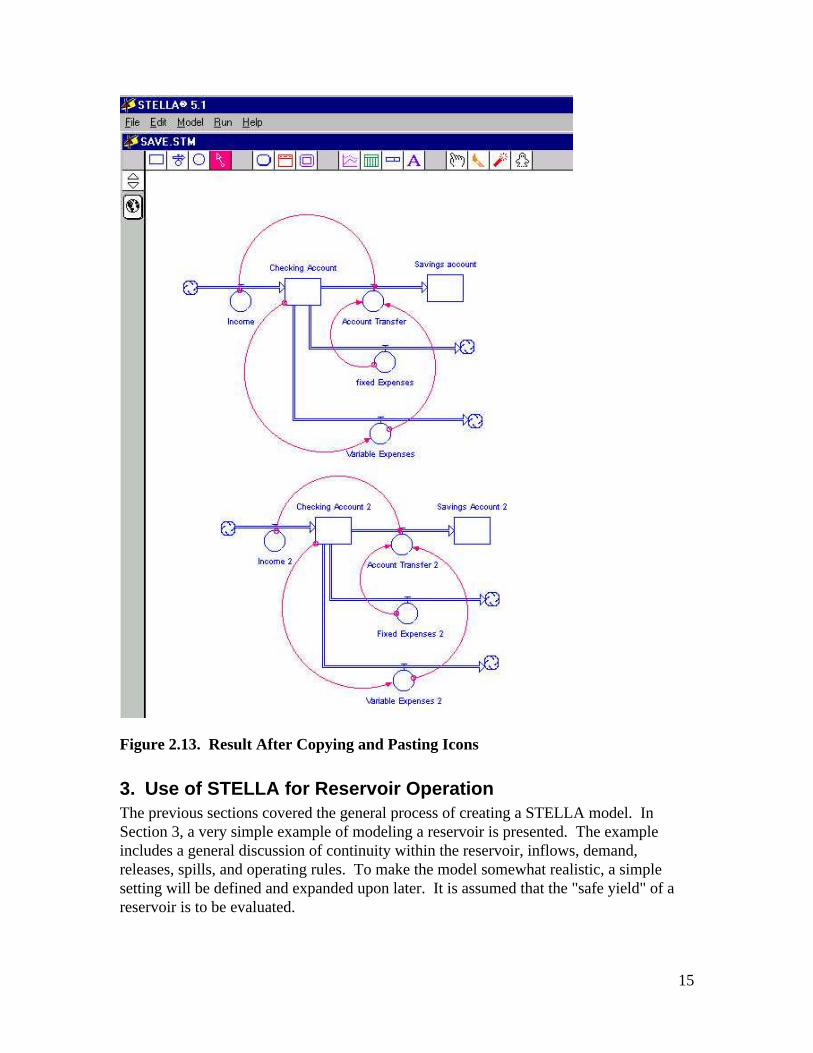
button. This results in a copy of the complete set of icons, including the functional
relationships (
Figure 2.13). Note that the only difference between the original and the copy is that a 2has been added to each of the duplicates names. STELLA requires each object to have aunique name, therefore the duplicates names are modified from the original. The new setof icons are independent objects which can be modified without affecting the originals.
15
Figure 2.13. Result After Copying and Pasting Icons
3. Use of STELLA for Reservoir OperationThe previous sections covered the general process of creating a STELLA model. InSection 3, a very simple example of modeling a reservoir is presented. The exampleincludes a general discussion of continuity within the reservoir, inflows, demand,releases, spills, and operating rules. To make the model somewhat realistic, a simplesetting will be defined and expanded upon later. It is assumed that the "safe yield" of areservoir is to be evaluated.
16
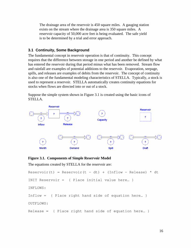
The drainage area of the reservoir is 450 square miles. A gauging stationexists on the stream where the drainage area is 350 square miles. Areservoir capacity of 50,000 acre feet is being evaluated. The safe yieldis to be determined by a trial and error approach.
3.1 Continuity, Some BackgroundThe fundamental concept in reservoir operation is that of continuity. This conceptrequires that the difference between storage in one period and another be defined by whathas entered the reservoir during that period minus what has been removed. Stream flowand rainfall are examples of potential additions to the reservoir. Evaporation, seepage,spills, and releases are examples of debits from the reservoir. The concept of continuityis also one of the fundamental modeling characteristics of STELLA. Typically, a stock isused to represent a reservoir. STELLA automatically creates continuity equations forstocks when flows are directed into or out of a stock.
Suppose the simple system shown in Figure 3.1 is created using the basic icons ofSTELLA.
Figure 3.1. Components of Simple Reservoir Model
The equations created by STELLA for the reservoir are:
Reservoir(t) = Reservoir(t - dt) + (Inflow - Release) * dt
INIT Reservoir = { Place initial value here… }
INFLOWS:
Inflow = { Place right hand side of equation here… }
OUTFLOWS:
Release = { Place right hand side of equation here… }
17
The first equation in the set is the continuity equation for the reservoir. At this stage inthe development of the model, the continuity equation states that the variableReservoir, is a function of its value at the previous time (t-dt) plus the differencebetween the Inflow and Release rate, times the time step (dt). As indicated by theequations, there is no initial value for storage and the inflows and outflows are not yetdefined.
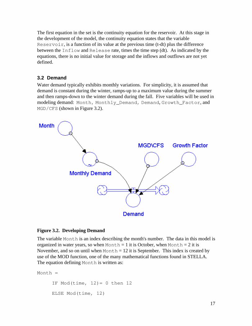
3.2 DemandWater demand typically exhibits monthly variations. For simplicity, it is assumed thatdemand is constant during the winter, ramps-up to a maximum value during the summerand then ramps-down to the winter demand during the fall. Five variables will be used inmodeling demand: Month, Monthly_Demand, Demand, Growth_Factor, andMGD/CFS (shown in Figure 3.2).
Figure 3.2. Developing Demand
The variable Month is an index describing the month's number. The data in this model isorganized in water years, so when Month = 1 it is October, when Month = 2 it isNovember, and so on until when Month = 12 it is September. This index is created byuse of the MOD function, one of the many mathematical functions found in STELLA.The equation defining Month is written as:
Month =
IF Mod(time, 12)= 0 then 12
ELSE Mod(time, 12)
18
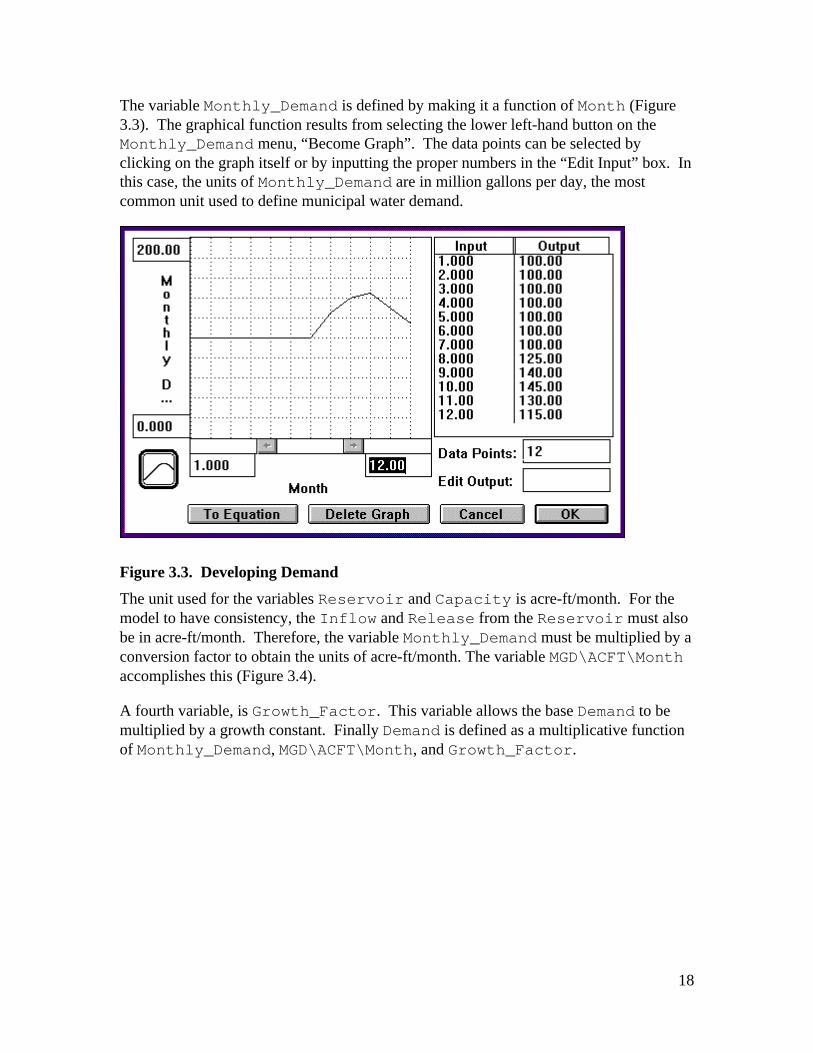
The variable Monthly_Demand is defined by making it a function of Month (Figure3.3). The graphical function results from selecting the lower left-hand button on theMonthly_Demand menu, “Become Graph”. The data points can be selected byclicking on the graph itself or by inputting the proper numbers in the “Edit Input” box. Inthis case, the units of Monthly_Demand are in million gallons per day, the mostcommon unit used to define municipal water demand.
Figure 3.3. Developing Demand
The unit used for the variables Reservoir and Capacity is acre-ft/month. For themodel to have consistency, the Inflow and Release from the Reservoir must alsobe in acre-ft/month. Therefore, the variable Monthly_Demand must be multiplied by aconversion factor to obtain the units of acre-ft/month. The variable MGD\ACFT\Monthaccomplishes this (Figure 3.4).
A fourth variable, is Growth_Factor. This variable allows the base Demand to bemultiplied by a growth constant. Finally Demand is defined as a multiplicative functionof Monthly_Demand, MGD\ACFT\Month, and Growth_Factor.

19
Figure 3.4. Defining the Converter MGD\ACT\Month
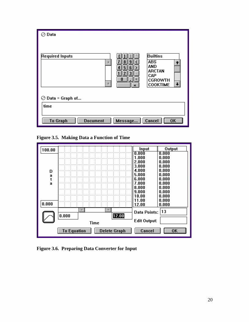
3.3 InflowsThis example uses thirty years of monthly streamflow data, placed in the variable Data.This is accomplished as follows:
First, have STELLA and EXCEL both operating, with EXCEL active and STELLA in thebackground. Copy thirty years of data (360 data points) from the EXCEL spreadsheetfile. While this data is in memory (on the clipboard), return to the STELLA model andopen the variable Data by double clicking on it. The variable Data is made a functionof time by typing "time" into the equation line, as shown in Figure 3.5.
Next, select the option "Become Graph" and a new window appears (Figure 3.6).Indicate that there are 361 data points (the first data slot is blank) by typing this into the“Data Points” box. Finally, highlight the Output column by clicking once on the“Output”. Use the Paste Command to insert the data into the column. The final resultshould appear as in Figure 3.7.
20
Figure 3.5. Making Data a Function of Time
Figure 3.6. Preparing Data Converter for Input
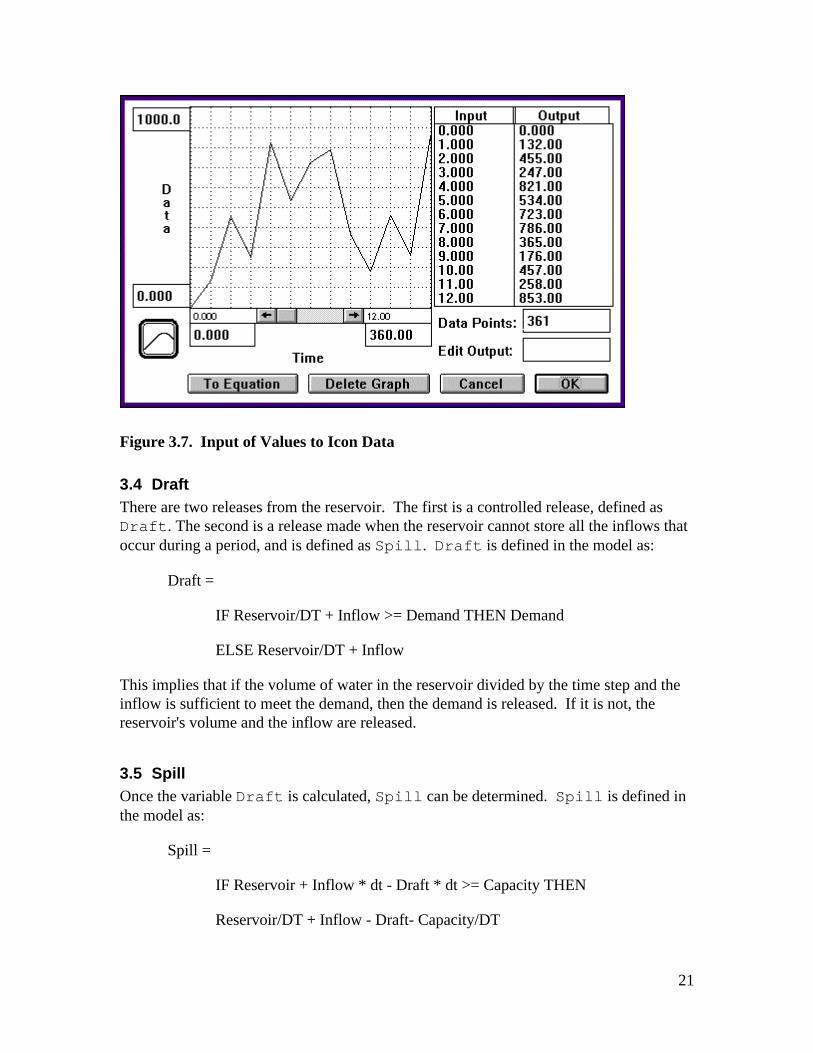
21
Figure 3.7. Input of Values to Icon Data
3.4 DraftThere are two releases from the reservoir. The first is a controlled release, defined asDraft. The second is a release made when the reservoir cannot store all the inflows thatoccur during a period, and is defined as Spill. Draft is defined in the model as:
Draft =
IF Reservoir/DT + Inflow >= Demand THEN Demand
ELSE Reservoir/DT + Inflow
This implies that if the volume of water in the reservoir divided by the time step and theinflow is sufficient to meet the demand, then the demand is released. If it is not, thereservoir's volume and the inflow are released.
3.5 SpillOnce the variable Draft is calculated, Spill can be determined. Spill is defined inthe model as:
Spill =
IF Reservoir + Inflow * dt - Draft * dt >= Capacity THEN
Reservoir/DT + Inflow - Draft- Capacity/DT
22
ELSE 0
This equation states that if the Reservoir volume plus the Inflow volume during theperiod (Inflow * dt) minus the Draft volume during the period (Draft * dt) isgreater than the Capacity, then a Spill is to be calculated. If it is not, the Spill isset equal to zero.
3.6 Operating RulesThe definitions for Draft and Spill stated above imply a very simple reservoiroperating policy. More complex policies can be developed in STELLA. Such rulesmight make the draft a function of time of year, the storage volume as a percent ofcapacity, or longer-term streamflow forecasts. One may wish to incorporate hedgingrules based upon the storage level of reservoirs or the total number of days of demand leftin storage.
3.7 Run Time Increment (DT)The value of DT defines the time step of the model. In the example, monthly streamflowvalues are entered as the driving data, and the basic time step is one month. This impliesthat when DT is set equal to 1, a monthly time step is being used. However, the value ofDT can be changed to a smaller value if desired. For instance, it may become necessaryto model the system at a weekly time step, and this can be accomplished by simplychanging the value of DT in the "Time Specs" Menu to 0.25. Values in the model arethen updated at a quarterly monthly rate. Details on DT are on pages 24-26 of theTechnical Documentation.
3.8 Maximum StorageIt is often necessary to define the maximum storage in a reservoir as a function of thetime of year. This is accomplished in the same fashion as illustrated with Demand.However, it is important to note precisely what STELLA does. If capacity is a timevariable, it indicates the maximum value of storage at the end of the period. It thereforecorresponds to the initial storage level at the beginning of the next time period. If theuser wishes the maximum storage value to control the storage level at the beginning ofthe period, the values of maximum storage should be shifted by one time period.
4. Advanced FeaturesAlthough it is very easy to use the STELLA simulation environment, the development ofcomplex models requires discipline and experience. For knowledgeable programmers,STELLA offers a wide range of productivity tools and other advantages over moreconventional programming environments. For novice modelers, STELLA offers theopportunity to develop simulation models with an ease not previously available. A
23
variety of features in STELLA aid both the experienced programmer and the novice.Some of these tools are discussed below.
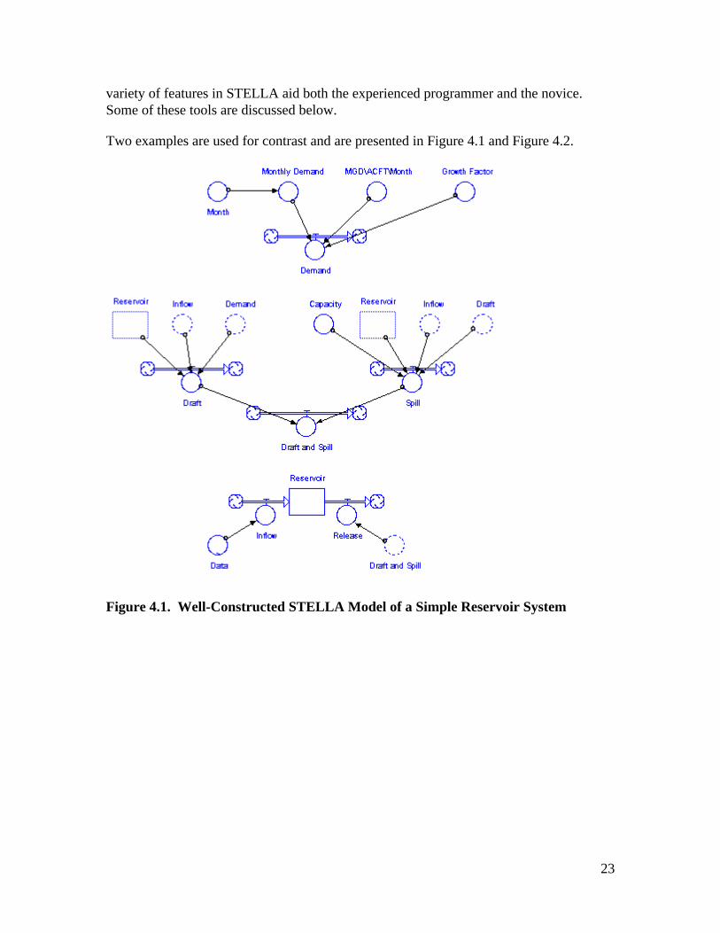
Two examples are used for contrast and are presented in Figure 4.1 and Figure 4.2.
Figure 4.1. Well-Constructed STELLA Model of a Simple Reservoir System
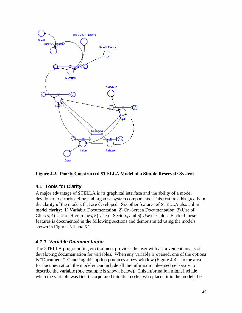
24
Figure 4.2. Poorly Constructed STELLA Model of a Simple Reservoir System
4.1 Tools for ClarityA major advantage of STELLA is its graphical interface and the ability of a modeldeveloper to clearly define and organize system components. This feature adds greatly tothe clarity of the models that are developed. Six other features of STELLA also aid inmodel clarity: 1) Variable Documentation, 2) On-Screen Documentation, 3) Use ofGhosts, 4) Use of Hierarchies, 5) Use of Sectors, and 6) Use of Color. Each of thesefeatures is documented in the following sections and demonstrated using the modelsshown in Figures 5.1 and 5.2.
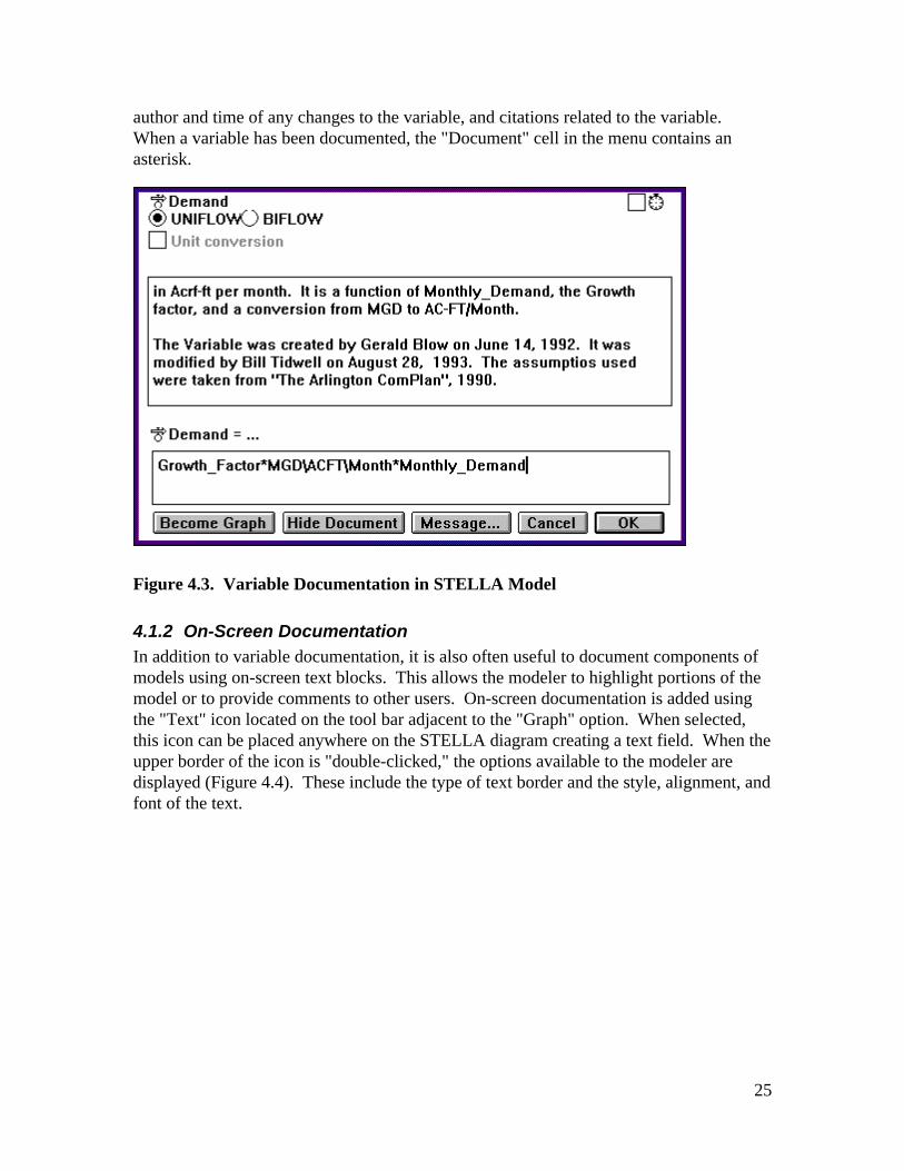
4.1.1 Variable DocumentationThe STELLA programming environment provides the user with a convenient means ofdeveloping documentation for variables. When any variable is opened, one of the optionsis "Document." Choosing this option produces a new window (Figure 4.3). In the areafor documentation, the modeler can include all the information deemed necessary todescribe the variable (one example is shown below). This information might includewhen the variable was first incorporated into the model, who placed it in the model, the
25
author and time of any changes to the variable, and citations related to the variable.When a variable has been documented, the "Document" cell in the menu contains anasterisk.
Figure 4.3. Variable Documentation in STELLA Model
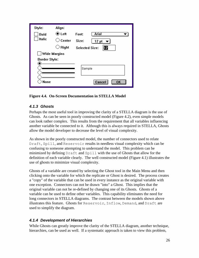
4.1.2 On-Screen DocumentationIn addition to variable documentation, it is also often useful to document components ofmodels using on-screen text blocks. This allows the modeler to highlight portions of themodel or to provide comments to other users. On-screen documentation is added usingthe "Text" icon located on the tool bar adjacent to the "Graph" option. When selected,this icon can be placed anywhere on the STELLA diagram creating a text field. When theupper border of the icon is "double-clicked," the options available to the modeler aredisplayed (Figure 4.4). These include the type of text border and the style, alignment, andfont of the text.
26
Figure 4.4. On-Screen Documentation in STELLA Model
4.1.3 GhostsPerhaps the most useful tool in improving the clarity of a STELLA diagram is the use ofGhosts. As can be seen in poorly constructed model (Figure 4.2), even simple modelscan look rather complex. This results from the requirement that all variables influencinganother variable be connected to it. Although this is always required in STELLA, Ghostsallow the model developer to decrease the level of visual complexity.
As shown in the poorly constructed model, the number of connectors used to relateDraft, Spill, and Reservoir results in needless visual complexity which can beconfusing to someone attempting to understand the model. This problem can beminimized by defining Draft and Spill with the use of Ghosts that allow for thedefinition of each variable clearly. The well constructed model (Figure 4.1) illustrates theuse of ghosts to minimize visual complexity.
Ghosts of a variable are created by selecting the Ghost tool in the Main Menu and thenclicking onto the variable for which the replicate or Ghost is desired. The process createsa "copy" of the variable that can be used in every instance as the original variable withone exception. Connectors can not be drawn "into" a Ghost. This implies that theoriginal variable can not be re-defined by changing one of its Ghosts. Ghosts of avariable can be used to define other variables. This capability eliminates the need forlong connectors in STELLA diagrams. The contrast between the models shown aboveillustrates this feature. Ghosts for Reservoir, Inflow, Demand, and Draft areused to simplify the diagram.
4.1.4 Development of HierarchiesWhile Ghosts can greatly improve the clarity of the STELLA diagram, another technique,hierarchies, can be used as well. If a systematic approach is taken to view this problem,
27
the model can be considered to perform three basic functions. First, demand is calculatedas a function of the appropriate variables. Next, Draft and Spill are calculatedsimilarly and combined into a single term. Finally, the variables Data and Demand andSpill are used to determine Inflow into the Reservoir, Reservoir_Storage,and total Release from the system.
Several features should be noted in the development of this hierarchy. In general, thediagram "flows" from the top to the bottom. In each "level" of this model, a differentactivity occurs. First, demand is calculated, then Draft and Spill, and finally theReservoir system is modeled. In this process, a number of initial variables are used tocalculate intermediate variables and then , finally, the most important variables. Thevariables of most interest, the Inflow, Release, and the Reservoir, are clearlypresented in the final level of the hierarchy without the clutter shown in the poorlyconstructed model. Anyone familiar with the notation of STELLA can easily follow thelogic of the model. The activities in the model also flow from left to right. Draft mustbe calculated before Spill, thus the cluster of variables defining Draft lie to the left ofthe cluster defining Spill.
The suggestions on developing hierarchies described above can greatly improve theclarity of a STELLA diagram. However, they are merely stylistic suggestions, not rules.With experience, a modeler using STELLA may develop other hierarchical protocol thatis equally clear. Whatever protocol is developed should be used consistently in themodel.
4.1.5 SectorsSectors within STELLA are a natural extension of hierarchies. In the previous section, itwas noted that "clusters" of variables form naturally in defining larger concepts in amodel. In more traditional programming languages such as FORTRAN, these clusters ofvariables might be located within a subroutine. When desirable, clusters can be formallygrouped into a collection using the Sector tool in the main menu. To make a Sector,select the Sector tool and place it on the diagram by clicking the mouse. Use the cornersto expand, contract, and/or move the sector to cover all of the desired variables.
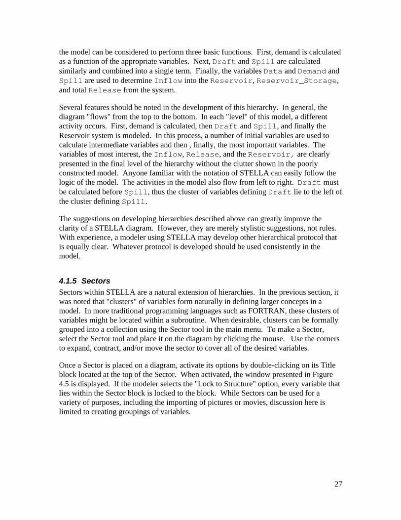
Once a Sector is placed on a diagram, activate its options by double-clicking on its Titleblock located at the top of the Sector. When activated, the window presented in Figure4.5 is displayed. If the modeler selects the "Lock to Structure" option, every variable thatlies within the Sector block is locked to the block. While Sectors can be used for avariety of purposes, including the importing of pictures or movies, discussion here islimited to creating groupings of variables.
28
Figure 4.5. Sector in STELLA Model
This process provides two helpful features. First, the variables within the Sector aremoved as a unit with the Sector, which greatly increases modeling efficiency whenworking with a large model. Second, Sectors can be run individually. This allows the"debugging" of a model sector by sector if desired, thus eliminating the need to completethe entire model before evaluating portions of the model. Details on Sectors are on pages6-31 to 6-38 of the Technical Documentation.
Note: If a sector relies on the value of a variable defined in another sector, and not allsectors are running, the results may be inaccurate and unexpected.
4.1.6 ColorTo improve model clarity, variable icons can be "painted" one of 256 different colors.Color can be used to define similar variables (for instance, painting all Inflows the samecolor) or to distinguish between different Sectors.
4.2 Sensitivity AnalysisModels are developed to answer questions related to relatively uncertain conditions. Thisis especially true in water resources modeling. For instance, the question of how demandfor water will change over time and how it will impact system performance arises often.STELLA provides the very convenient and powerful option of allowing a modeler or userto explore how changes in variables impact other variables. The user is able to select avariable for which a sensitivity analysis is desired, specify the number of runs of themodel, and the range of values the variable is to assume.
29
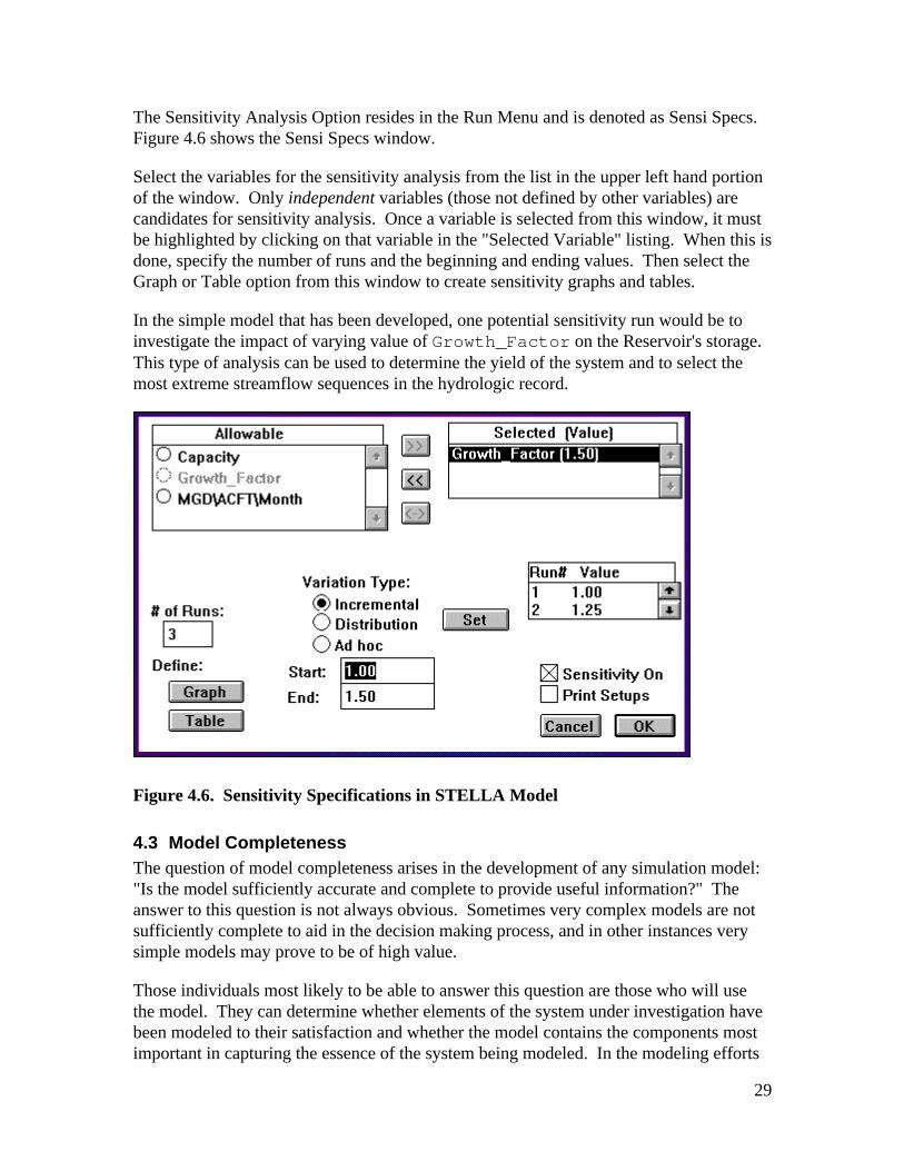
The Sensitivity Analysis Option resides in the Run Menu and is denoted as Sensi Specs.Figure 4.6 shows the Sensi Specs window.
Select the variables for the sensitivity analysis from the list in the upper left hand portionof the window. Only independent variables (those not defined by other variables) arecandidates for sensitivity analysis. Once a variable is selected from this window, it mustbe highlighted by clicking on that variable in the "Selected Variable" listing. When this isdone, specify the number of runs and the beginning and ending values. Then select theGraph or Table option from this window to create sensitivity graphs and tables.
In the simple model that has been developed, one potential sensitivity run would be toinvestigate the impact of varying value of Growth_Factor on the Reservoir's storage.This type of analysis can be used to determine the yield of the system and to select themost extreme streamflow sequences in the hydrologic record.
Figure 4.6. Sensitivity Specifications in STELLA Model
4.3 Model CompletenessThe question of model completeness arises in the development of any simulation model:"Is the model sufficiently accurate and complete to provide useful information?" Theanswer to this question is not always obvious. Sometimes very complex models are notsufficiently complete to aid in the decision making process, and in other instances verysimple models may prove to be of high value.
Those individuals most likely to be able to answer this question are those who will usethe model. They can determine whether elements of the system under investigation havebeen modeled to their satisfaction and whether the model contains the components mostimportant in capturing the essence of the system being modeled. In the modeling efforts
30
for the Portland Water Bureau, extensive efforts were made to ensure the models wouldbe useful to units of the Bureau and the various stakeholders interested in water resourcesand reservoir management.
4.4 Modeling of System PerformanceThe water resources models developed in this study were designed to aid in selecting thebest management strategies for the region. This can be accomplished by evaluatingsystem performance under the status quo and then investigating performance under avariety of alternatives. Selection of the proper measures of system performance is afunction of who will use the models and how they will be used. Common measures ofsystem performance can be categorized into four areas: 1) System reliability, 2)Biological impacts, 3) Economic impacts, and 4) Political impacts.
4.4.1 System ReliabilityThree common measures are used to evaluate system reliability. Typically reliability issimply considered the frequency with which a goal is met. For water supply, reliabilitymight be defined as the number of months in which demand is met divided by the numberof months of investigation. Two other measures are also important. One is systemresilience, defined here as the average length of time required for the system to return toan acceptable state of performance. The final measure is vulnerability, defined here asthe maximum deviation of performance measures from target values.
Although these three measures are often used to describe the performance of a systemrelative to meeting municipal and industrial water demand, they can also be used tomeasure the performance in meeting in-stream flow requirements or other target flows.
4.4.2 Biological ImpactsIt is quite feasible to model biological impacts in the STELLA environment. However, itis difficult to include biological impacts in the models discussed here because biologicalimpacts of interest in this problem are not well understood; also, no functionalrelationships exist between the flow in a river and fish production and the true quality offish habitat. Instead of directly modeling biological impacts, surrogates for biologicalimpacts have been chosen. These surrogates are the flow in the river during the year atcertain points throughout the system. Although it is recognized that flow is only asurrogate for the biological health of a river and the fish population that inhabit it, thisapproach was used due to the limited amount of data available.
4.4.3 Economic ImpactsThe shortfall of water creates many impacts. These impacts include lost revenue bymunicipalities, the loss of consumer surplus on the part of water purchasers, the negativeimpacts of outdoor vegetation, decreased fish production in streams, and a host of others.However, quantification of these impacts is extremely difficult, due to regional and
31
temporal variations in the impacts. For some items, such as fish production, theassignment of an economic loss term is complicated due to the loss of many nonquantified impacts, such as those on culture and religion. In the models developed, somenon-monetary impacts will be tracked but no attempt was made to convert them to dollarvalues. This does not imply that economic impacts can not be estimated or that this is notimportant.
4.4.4 Political and Social ImpactsThe environment in which decisions are made relating to water supply is influenced asoften by political concerns as it is by engineering analysis. Because water supply projectsare typically large in scope and impact many people in the community, the acceptance ofthe project by the public is extremely important.
The robustness of a water supply system and its ability to deliver low priced, high quality,and reliable water also reflects well on those whom the public perceive as responsible forthe system. If a water system can not meet water contracts, or if the reliability of thewater supply is called into question, public officials may be the target of extremecriticism and their positions may be placed in jeopardy.
There is little science or experience in modeling the political and social impacts of watersupply shortages. This does not imply, however, that such impacts are unimportant orthat decisions related to water supply may not be made on this basis. It is not anticipatedthat political indices will be developed in the STELLA models for the Bull Run Riverbasin. Measures such as the number, length, magnitude, and timing of shortfalls could, ina cursory sense have been made to reflect political impacts.
4.5 Programming LessonsIn the development of the STELLA models for this and other similar projects, a numberof lessons have been learned. Some of these lessons are of a general nature and othersrelate specifically to STELLA. Some of these lessons are specified below.
4.5.1 General Lessons
4.5.1.1 Good models start with clear study objectivesWhen initiating a water resources model using STELLA, there is a great temptation tobegin the modeling process early and devote a great deal of attention to the model.Perhaps the best advice is to not begin modeling until clear planning objectives have beenestablished. Although this advice seems obvious, it is surprising how difficult it is todevelop clear and concise planning objectives and then develop a model that addressesthose objectives. All to often the planning objectives play second chair to the model, andthus the model may prove unable to answer them definitively.
32
4.5.1.2 Good models continue with a definition of what is important in thesystemWhen good planning models are developed, it is much easier to see what is actuallyimportant in a system. Without planning objectives, one may be forced to model everydetail in a system since they may not know what is and isn't important. With goodplanning objectives, components in a model and their impact on the planning objectivescan be estimated and measured. Greater emphasis can be placed on those components ofmost importance.
4.5.1.3 Time allocation during modeling effortA common error in the development of a model is to devote too much time to thedevelopment of a model and too little to the calibration and verification of the model andthe generation of meaningful analysis. This may require that the model is not as complexas if all the effort was devoted to model development, but the value of the model will begreatly increased if time is apportioned to these other tasks.
4.5.1.4 Model ClarityIt is very important for those constructing models to remember they are likely the leastimportant person who will use the model from a decision-making context. The ultimateusers of the model should always be in the forefront of the modeler's consciousness andevery attempt should be made to create a model that they will find clear and easy to use.The use of Ghosts, Hierarchies, Sectors, and Color are just four of the techniquesmentioned in this report that aid in model clarity.
4.5.1.5 Simplicity vs. ComplexityThere appears to be a tendency among modelers toward complexity rather than simplicity.This is not surprising, given the educational background of most modelers and thecommon desire to make a model as complete as possible. Complex models shouldalways develop from simple models. Components should, in general, be left out ofmodels unless it is clear that their inclusion improves the ultimate value of the model.Simple models have the tendency to become complex with little encouragement.Modelers should always start simple, and make complex only those components whereinthere lies a clear value to do so.
4.5.2 STELLA Lessons
4.5.2.1 Non-negativity requirementsSTELLA offers the option of preventing a stock from going negative. This option is adefault option of a newly created stock. Although this concept seems quite reasonable, itis important in developing water resource models that the non-negativity option never
33
be used. Use of this option modifies the normal calculation of stocks and their outflowsand can create surprising results that are difficult to track.
4.5.2.2 Discrete vs. Continuous data and graphsSTELLA offers the option of representing data as either continuous or discrete. When the"Become Graph" option is selected, continuous data is shown as connected points anddiscrete data as bar lines. When the continuous data option is chosen, STELLA linearlyextrapolates between the points to find their value when a DT of less than one is used.This feature may or may not be appropriate for a given setting. For instance, if monthlydata is being used in a model and the value of DT is set to 0.25, should continuous (inwhich linear extrapolations will be made between points) or discrete (in which the sameflow is assumed to occur during the entire period) be chosen? This must be answered bya modeler who is aware of the implications.
4.5.2.3 Beginning and ending storages vs. end of period valuesWhen creating tables in STELLA, the modeler has the option to store either the value of astock at either the beginning or the end of a period. When developing continuityequations for system components and "verifying" that a model is working properly, it isimportant to know which value (beginning or ending) is being reported.
4.5.2.4 Variable Naming ConventionsAs has been emphasized, clarity is an important feature in any large or complex STELLAdiagram. One technique not previously mentioned to aid in model clarity is in theconvention chosen for naming variables. Variable names should be concise, intuitive,and descriptive. Avoid generic names like Reservoir and Flow. This permits the userto locate all information pertaining to a specific location without extensive searching.However, if the place identifier is too long, the type of data will not show in all lists ofvariables provided by STELLA.
An alternative (and equally valid) naming convention could place the type of data first,followed by the place identifier. For instance, rather than naming the building blocks forrelease from Dam1 and Dam 2, Dam1Release and Dam2Release, it may proveeffective to name them ReleaseDam1 and ReleaseDam2. In this way, anywhere inwhich variables are listed alphabetically, all flow icons would appear together, and couldbe located quickly in a table or graph menu. This convention could be applied to allvariable types that are repeated in a model such as flows, reservoirs, releases, spills, anddraft.
4.5.2.5 Limits on Input DataA flow or converter in STELLA can only contain 1500 values. This does not mean that ahistoric streamflow record with more than 1500 values can not be used. One approach tothis problem is to divide the historic data into several flow icons, each containing the
34
maximum number of values. A separate icon, linked to each of these data icons, can thenbe used to select the appropriate flows based on the current time period.
4.5.2.6 Impacts on Changing Time StepsThe numerical analysis techniques incorporated into STELLA solve differential equationsapproximately. The quality of the approximation is a function of the technique chosenand the time step. Users should be aware that if large time steps are chosen, results willbe less accurate. There is a trade-off between the speed at which the model runs and theaccuracy of the results.
Changing the time step (the value of DT) defines the accuracy of the results. It is goodpractice to run a model at various values of DT to determine if changes in DT results insignificantly large changes in the results to cause concern. It should be remembered, asnoted in the STELLA Technical Documentation that the value of DT should be a value of
(1/2)n (that is: .5, .25, .125, .0625, .03125).
4.5.2.7 Printing and PagesPrinting the STELLA diagrams is often necessary. This is accomplished by simplyselecting the Print Option in the File Menu in the main STELLA window. The user canalter the printout in two ways. Under the File Menu, the user can select the PAGESETUP option. This allows the diagram to be printed in either the Portrait or Landscapemode, with percentage reductions or enlargements. These modifications will not affectthe operations of the STELLA model but will change the manner in which it is paginated.
To preview the pagination of a diagram before printing, the user should select the "ShowPages" option found in the Diagram Preferences dialogue box under the EDIT Menu."Zooming out" (see section 3.5 of this guide) allows the user to see as much of thediagram on the computer screen as is desired.
5. Dynamic Data ExchangeA new feature in STELLAII called “Dynamic Data Exchange” (DDE). DDE allows theSTELLAII program to access data stored in another application program. These otherapplication programs include databases and spreadsheet programs such as MicrosoftEXCEL that support DDE and are a more appropriate in a tool for storing large qualitiesof data. This tool is useful when scenarios are run in STELLA which require only a smallportion of the data that exist in a spreadsheet or data base. The DDE can also be used toexport data from a STELLA run into a spreadsheet where more advance statisticalanalysis can be performed.
The information outline below comes High Performance Technical DocumentationSupplement for Dynamic Data Exchange (DD), Help Files and Import Sensitivity Setupand is supplemented with notes.
35
5.1 General RulesCreating links between Stella and a spreadsheet or database is relatively simple processalthough some general rules apply. These apply anytime you establish a DDE link.
• Each link will consist of a server, the file that generates the data, and a client, thefile that will receive the data.
• Save both the STELLAII file and the file in the other application before creatinga DDE link. The link will use the file names to describe the connection. Anychanges to the names of the files after the link is forged will prevent the re-establishment of the link when the files are subsequently opened.
• Creating links from the STELLAII file to a V file is not possible (all links mustgo through another application).
• Both the server (data originator) and the client (data recipient) files must be openfor a change in the server to be registered by the client. The update occurs at thetime of a change and not when the files are opened, so make should that both areopen before making any changes, Note that when a change is made to a largespreadsheet, time may be required to update the calculations. The link will takeplace after the calculations in the spreadsheet are complete. If an EXCELspreadsheet does not appear to be updating press F9 and then wait for thecalculations to be completed. At this time the link will update.
• The number of links will be limited by the amount of RAM you have on yourmachine. High performance does not recommend more than 250-300 links. Forlarge models and spreadsheets at lest 24 MG Ram is needed.
5.2 STELLAII as a clientTo create a link that brings data into a STELLAII model the following rules apply:
• Graphical functions, converters with no inputs or builtins, flows with no inputs orbuiltins, Reservoir initial values, and Queues can act as clients for DDEinterchange. (Graphical functions are limited to 1500 data points and otherequation dialogs are limited to 2000 characters)
• TO establish the link, you’ll need to first copy the data from the other application.Then open the appropriate dialog in STELLAII. (If you are using a graphicalfunction, click on the Output column header to highlight the entire column.)Next, use the key command control-V to paste the data set into STELLAII (theEdit menu is not available within a dialog). Once you paste, you will get asecondary dialog in which you can choose to paste either the data or the link.Choose Paste Link and click OK.
• Whenever you’re in a dialog that has a DDE link, be sure to exit the dialog withOK. Exiting via cancel will cause you to cancel (i.e. Break) the DDE link.
• If you subsequently open a model which contains links, the software will help youreestablish links and open the server. Note if the server is not in the correct pathSTELLAII will not be able to find the server.
• Note whenever opening a STELLAII to which you wish to reestablishlinks, you should always open the server (spreadsheet or data base) before
36
opening STELLAII. Failure to do so may cause your system to lock up. Ifyou are not going to reestablish links you do not need to have the serveropen.
5.3 STELLAII as a serverTo create a link which exports data from a STELLAII model the following rules apply:
• Output data from Tables acts as a server for DDE interchange.• To establish the link, copy the data you are interested in linking by clicking on the
column or row header and choosing Copy under the Edit menu.• Navigate to the other application and choose Paste Special or Paste Link (usually
from the Edit menu).• If you subsequently open a file which contains links to a STELLAII model you
must open the model first.• Note very large DDE transfers from STELLAII to EXCEL have caused
errors in which all of the data is not correctly transferred. An alternative tousing DDE is to save a STELLAII Table as text (.txt) and then openingand saving that file from within EXCEL.