Embed Size (px)
Citation preview

Svensk Kärnbränslehantering ABSwedish Nuclear Fueland Waste Management CoBox 5864SE-102 40 Stockholm SwedenTel 08-459 84 00
+46 8 459 84 00Fax 08-661 57 19
+46 8 661 57 19
Technical Report
TR-99-13
Site-scale groundwater flowmodelling of Ceberg
Douglas Walker
Duke Engineering & Services
Björn Gylling
Kemakta Konsult AB
June 1999

Keywords: Canister flux, computer modelling, F-ratio, groundwater flow,Monte Carlo simulation, repository, stochastic continuum, SR 97, travel time.
This report concerns a study which was conducted for SKB. The conclusionsand viewpoints presented in the report are those of the author(s) and do notnecessarily coincide with those of the client.
Site-scale groundwater flowmodelling of Ceberg
Douglas Walker
Duke Engineering & Services
Björn Gylling
Kemakta Konsult AB
June 1999
ISSN 1404-0344CM Gruppen AB, Bromma, 1999
i
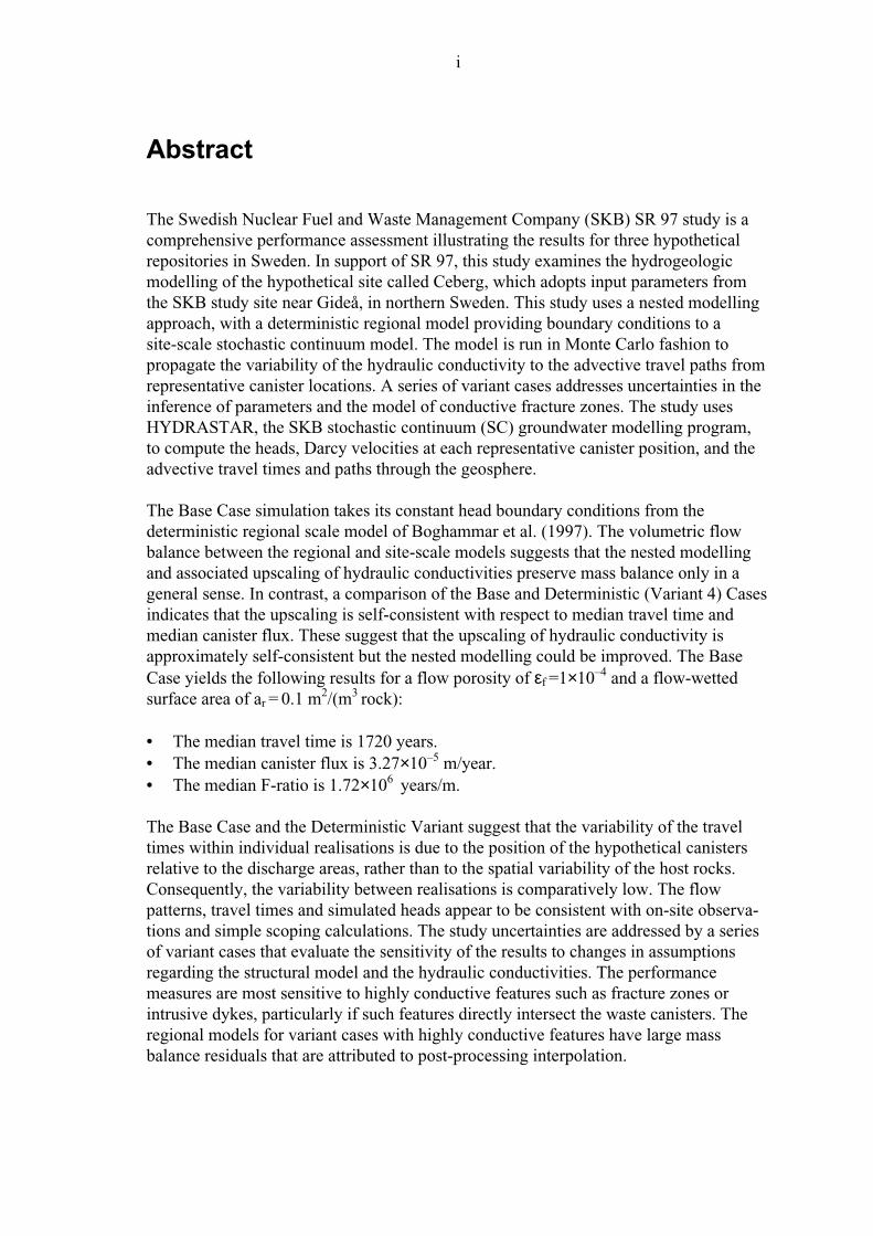
Abstract
The Swedish Nuclear Fuel and Waste Management Company (SKB) SR 97 study is a
comprehensive performance assessment illustrating the results for three hypothetical
repositories in Sweden. In support of SR 97, this study examines the hydrogeologic
modelling of the hypothetical site called Ceberg, which adopts input parameters from
the SKB study site near Gideå, in northern Sweden. This study uses a nested modelling
approach, with a deterministic regional model providing boundary conditions to a
site-scale stochastic continuum model. The model is run in Monte Carlo fashion to
propagate the variability of the hydraulic conductivity to the advective travel paths from
representative canister locations. A series of variant cases addresses uncertainties in the
inference of parameters and the model of conductive fracture zones. The study uses
HYDRASTAR, the SKB stochastic continuum (SC) groundwater modelling program,
to compute the heads, Darcy velocities at each representative canister position, and the
advective travel times and paths through the geosphere.
The Base Case simulation takes its constant head boundary conditions from the
deterministic regional scale model of Boghammar et al. (1997). The volumetric flow
balance between the regional and site-scale models suggests that the nested modelling
and associated upscaling of hydraulic conductivities preserve mass balance only in a
general sense. In contrast, a comparison of the Base and Deterministic (Variant 4) Cases
indicates that the upscaling is self-consistent with respect to median travel time and
median canister flux. These suggest that the upscaling of hydraulic conductivity is
approximately self-consistent but the nested modelling could be improved. The Base
Case yields the following results for a flow porosity of εf =1×10⁻⁴
and a flow-wetted
surface area of ar = 0.1 m2/(m
3 rock):
• The median travel time is 1720 years.
• The median canister flux is 3.27×10⁻⁵
m/year.
• The median F-ratio is 1.72×10⁶
years/m.
The Base Case and the Deterministic Variant suggest that the variability of the travel
times within individual realisations is due to the position of the hypothetical canisters
relative to the discharge areas, rather than to the spatial variability of the host rocks.
Consequently, the variability between realisations is comparatively low. The flow
patterns, travel times and simulated heads appear to be consistent with on-site observa-
tions and simple scoping calculations. The study uncertainties are addressed by a series
of variant cases that evaluate the sensitivity of the results to changes in assumptions
regarding the structural model and the hydraulic conductivities. The performance
measures are most sensitive to highly conductive features such as fracture zones or
intrusive dykes, particularly if such features directly intersect the waste canisters. The
regional models for variant cases with highly conductive features have large mass
balance residuals that are attributed to post-processing interpolation.

ii
Sammanfattning
SR 97 är en säkerhetsanalys av tre hypotetiska djupförvar i Sverige. Denna rapport,
utförd som en del av SR 97, beskriver den hydrogeologiska modelleringen av Ceberg.
Ceberg är en hypotetisk plats där indata och parametrar baseras på förhållanden vid en
plats där SKB utfört undersökningar i närheten av Gideå, som är beläget i norra Sverige.
I den här beräkningsstudien har en nästlad modellering använts där en deterministisk
regional modell ger randvillkor till en stokastisk kontinuum modell i platsskala. Monte
Carlo simulering har använts för att propagera variabiliteten i hydraulisk konduktivitet
till advektiva partikelbanor som utgår från representativa kapselpositioner. I en serie
varianter har osäkerheter vid tolkandet av parametrar och överförandet av randvillkor
analyserats. För att beräkna tryck, Darcy-hastigheter (specifkt flöde) vid kapsel-
positioner, advektiva gångtider samt partikelbanor genom geosfären har SKB:s
stokastiska kontinuumprogram för grundvattenmodellering, HYDRASTAR, använts.
I basfallet har randvillkor i form av tidsoberoende tryck från en deterministisk regional
modell (Boghammar et al., 1997) använts. Överensstämmelsen i flödesbalanserna
mellan den regionala modellen och modellen i platsskala indikerar att den nästlade
modelleringen och den därvid använda uppskalningen av hydrauliska konduktiviteter
endast bevarar massbalansen i en generell mening. En jämförelse mellan basfallet och
det deterministiska fallet indikerar emellertid att uppskalningen av hydrauliska
konduktiviteter ger konsistenta resultat för medianvärden av gångtider och specifkt
flöde vid kapselpositioner. Detta indikerar att uppskalningen approximativt ger det
eftersträvade resultatet, men att den nästlade modelleringen kan förbättras. Resultaten
för basfallet ger mätetal för förvarsfunktionen i Ceberg enligt följande när flödes-
porositeten εf = 1×10⁻⁴
och flödesvätta ytan ar = 0.1 m2
/(m3
rock) används:
• Medianen för gångtiderna är 1720 år
• Medianen för specifkt flöde vid kapselpositioner är 3.27×10⁻⁵ m/år
• Medianen för F-faktorn är 1.72×10⁶ år/m
Basfallet och den deterministiska varianten indikerar att variabiliteten i gångtider inom
en enskild realisering beror av läget på den hypotetiska kapseln relativt utströmnings-
områden snarare än den rumsliga variabiliteten i det omgivande berget. Därmed blir
variabiliteten i de beräknade mätetalen mellan olika realiseringar förhållandevis låg.
Flödesmönstren, gångtider och simulerade tryck är i överensstämmelse med observa-
tioner gjorda på platsen och med förenklade överslagsberäkningar. Osäkerheter i studien
behandlas genom att utföra en serie av varianter för att utröna känsligheten i resultat
relaterat till ändringar i strukturmodellen och konduktivitetsvärden. Mätetalen för
förvarsfunktionen påverkas i hög grad av förekomst av högkonduktiva strukturer i form
av sprickzoner eller intrusioner, speciellt om dessa strukturer träffar kapselpositioner.
De regionala modellerna för de variationsfall där konduktiviteten har ökats för
strukturerna är behäftade med stora residualer i massbalanserna. Residualerna
uppkommer i efterbehandlingsprocessen där massbalanserna uppskattas genom
interpolation.

v
Contents
Abstract i
Sammanfattning iii
Contents v
List of Figures ix
List of Tables xv
1 Introduction 1
1.1 SR 97 1
1.2 Study Overview 1
2 Modelling Approach 3
2.1 The PA Model Chain 3
2.2 HYDRASTAR 4
2.3 Development of Modelled Cases 7
3 Model Application 9
3.1 Site Description 9
3.2 Hydrogeology 10
3.3 Regional Model and Boundary Conditions 11
3.4 Model Grid and Repository Layout 14
3.5 Input Parameters 17
3.5.1 Site-Scale Conductor Domain (SCD) 18
3.5.2 Site-Scale Rock Domain (SRD) 20
3.5.3 Geostatistical Model 20
3.5.4 Other Parameters 24
4 Base Case 27
4.1 Monte Carlo Stability 27
4.2 Boundary Flux Consistency 29
4.3 Ensemble Results 32
4.3.1 Travel Time and F-ratio 32
4.3.2 Canister Flux 36
4.3.3 Flow Pattern and Exit Locations 38
4.3.4 Validity of Results 42

vi
4.4 Individual Realisations 43
4.5 Individual Starting Positions 50
5 Variant Cases 59
5.1 Increased Conductivity Contrast 61
5.2 Alternative Conductive Features 69
5.3 Increased Conductivity Variance 78
5.4 Deterministic Simulation 86
6 Discussion and Summary 91
6.1 Input Data 91
6.2 Base Case 92
6.3 Variant Cases 94
6.3.1 Increased Conductivity Contrast 94
6.3.2 Alternative Conductive Features 94
6.3.3 Increased Conductivity Variance 95
6.3.4 Deterministic Simulation 95
6.3.5 Comparison 96
6.4 Possible Model Refinements 98
6.5 Summary of Findings 98
Acknowledgements 101
References 103
Appendix A. Definition of Statistical Measures 109
A.1 Floating Histograms 109
A.2 Statistical Significance of the Comparison of Distributions 109
Appendix B. Supplemental Regional Simulation 111
B.1 Variant 2 Regional Model 111
B.1.1 Introduction 111
B.1.2 Alternative Conductive Features (GRSFX) 111
B.2 Regional Model Mass Balance Calculations 112
Appendix C. Supplemental Calculations 115
C.1 Upscaling of Hydraulic Conductivity Model 115
C.1.1 Approach 115
C.1.2 Base Case (35 m scale) Model 115
C.2 Scoping Calculation for Approximate Travel Times 117
C.2.1 Approach 117
C.2.2 Application 118
vii
Appendix D. Summary of Input Parameters 119
Appendix E. Data Sources 121
E.1 SICADA Logfile for Coordinates and 25 m Interpreted K Values 121
E.2 SICADA Logfile for Coordinates, 2 m and 3 m Interpreted K Values 121
E.3 Structural Data 122
E.4 Repository Lay-out 123
E.5 Boundary Conditions 123
E.6 File Locations 124
Appendix F. Additional Software Tools 125
Appendix G. HYDRASTAR Input file for Base Case 129
Appendix H. Coordinate Transforms 135

ix
List of Figures
Figure 2.1-1 SKB PA model chain. 4
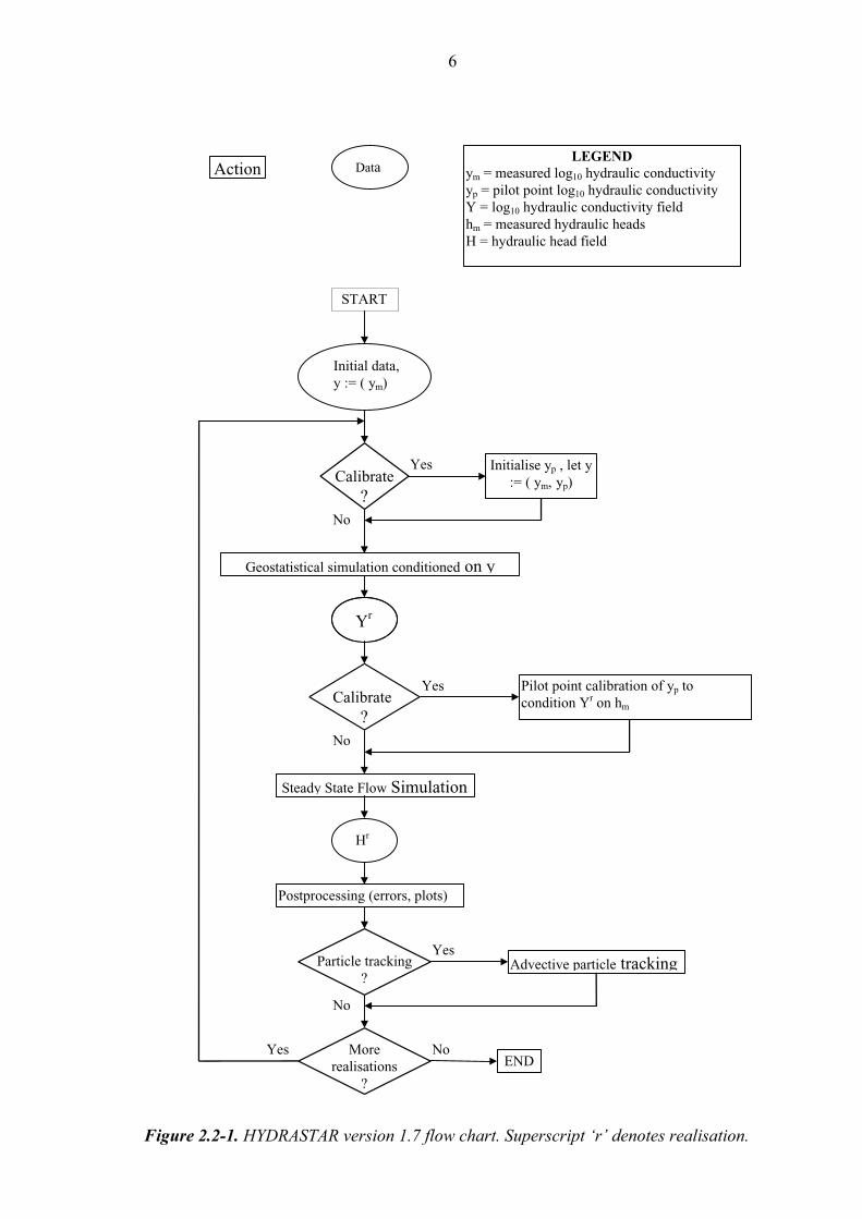
Figure 2.2-1 HYDRASTAR version 1.7 flow chart. Superscript ‘r’ denotes
realisation. 6
Figure 3.1-1 Location of the Gideå site. Dashed line represents roads. 10
Figure 3.3-1 Gideå site map, showing the large and small regional models of
Boghammar et al. (1997) in green and yellow, respectively. The
site-scale model is shown in red. 12
Figure 3.3-2 Constant head boundary conditions for each face of the model
domain for Ceberg (hydraulic head, in metres). 13
Figure 3.4-1 Gideå site-scale model domain (blue line). Tunnels of the
hypothetical repository at –500 masl are shown projected to
ground surface (scale in metres). 15
Figure 3.4-2 Ceberg hypothetical repository tunnel layout at –500 masl.
Numbered locations are 119 stream tube starting locations as
representative canister positions. 16
Figure 3.5-1 Gideå boreholes. Coordinates are a local system used in the KBS-3
study. 18
Figure 3.5-2 Ceberg site-scale conductor domains (SCD) after Hermansson et al.
(1997) and Saksa and Nummela (1998). 19
Figure 3.5-3 Semivariograms of log10 hydraulic conductivity for Ceberg rock
domain (SRD), for packer test data (25 m), INFERENS-fitted
(50 m), and interpolated (35 m). 21
Figure 3.5-4 HYDRASTAR representation of Ceberg conductive fracture zones
(SCD1). Coordinates are RAK system offset by 1,650,000 m in
east-west and 7,030,000 m in north-south (view from above, with
RAK North in the y-positive direction, scale in metres). 22
Figure 3.5-5 Log10 hydraulic conductivity on the upper model surface, Ceberg
Variant 4 (deterministic representation of hydraulic conductivity, in
plan view, with RAK North in the y-positive direction, scale in
metres). 23
Figure 3.5-6 Log10 of hydraulic conductivity for one realisation of Ceberg Base
Case. Upper image is plan view, with North in the y-positive
direction, scale in metres. Lower image is elevation view of the
same field, looking North. 24
Figure 4.1-1 Monte Carlo stability in the Ceberg Base Case. Median travel time
versus number of realisations. Results are shown for 119 starting
positions, a flow porosity of εf = 1×10⁻⁴
and travel times less than
100,000 years. 28

x
Figure 4.1-2 Monte Carlo stability in the Ceberg Base Case. Median canister
flux versus number of realisations. Results are shown for 119
starting positions. 28
Figure 4.2-1 Consistency of Ceberg boundary flow, regional versus site-scale
models. The arithmetic mean flow for five realisations of the site-
scale model is shown in parentheses. Arrows denote the regional
flow direction. 30
Figure 4.3-1 Relative frequency histogram of log10 travel time for Ceberg Base
Case. Results are shown for 100 realisations of 119 starting
positions and a flow porosity of εf = 1×10⁻⁴
. 33
Figure 4.3-2 Travel times by realisation for Ceberg Base Case. Results are
shown for 119 starting positions and a flow porosity of εf = 1×10⁻⁴
. 34
Figure 4.3-3 Number of realisations with travel times less than 1000 years
(squares) and 100,000 years (lines), by stream tube number for
Ceberg Base Case. Results are shown for 100 realisations of 119
starting positions and a flow porosity of εf = 1×10⁻⁴
. 35
Figure 4.3-4 Relative frequency histogram of log10 F-ratio for Ceberg Base Case.
Results are shown for 100 realisations of 119 starting positions,
a flow porosity of εf = 1×10⁻⁴
and a flow-wetted surface of
ar = 0.1 m2/(m
3 rock). 36
Figure 4.3-5 Relative frequency histogram of log10 canister flux for Ceberg
Base Case. Results are shown for 100 realisations of 119 starting
positions. 37
Figure 4.3-6 Box plot of log10 canister flux for Ceberg Base Case, by realisation.
Results are shown for 119 starting positions. 37
Figure 4.3-7 Log10 travel time versus log10 canister flux for Ceberg Base Case.
Results are shown for 100 realisations of 119 starting positions and
a flow porosity of εf = 1×10⁻⁴
. 38
Figure 4.3-8 Stream tubes in one realisation of the Ceberg Base Case.
Conductive fracture zones (CD) are represented as planes (view
from above, with North in the y-positive direction, scale in metres). 39
Figure 4.3-9 Exit locations for Ceberg Base Case, 100 realisations of 119
starting positions. Repository tunnels at –500 masl shown projected
up to the model surface (plan view, scale in metres). 40
Figure 4.3-10 Discharge areas and exit locations for the Ceberg Base Case.
Results are shown for 100 realisations of 119 starting positions
(plan view, scale in metres). 41
Figure 4.3-11 Floating histogram of log10 travel time for stream tubes exiting to
the discharge areas shown in Figure 4.3-10. Results are shown for
100 realisations of 119 starting positions and a flow porosity of
εf = 1×10⁻⁴
. 41
xi
Figure 4.3-12 Exit locations on the southern model surface for the Ceberg Base
Case. Results are shown for 100 realisations of 119 starting
positions (elevation view looking North, scale in metres). 42
Figure 4.4-1 Stream tubes in realisation number 1 of Ceberg Base Case. The
y-positive axis of a) is rotated cw from North. Results are shown
for 119 starting positions and a flow porosity of εf = 1×10⁻⁴
. 44
Figure 4.4-2 Stream tubes for Ceberg Base Case realisation numbers 1 through
3, plan view (looking downward). Results are shown for 119
starting positions and a flow porosity of εf = 1×10⁻⁴
. (Not to scale;
refer to Figure 4.4-1 for legend). 45
Figure 4.4-3 Realisations 1, 2, and 3 of the Ceberg Base Case, floating
histograms of log10 travel time (upper plot) and log10 canister flux
(lower plot). Results are shown for 119 starting positions and a
flow porosity of εf = 1×10⁻⁴
. 48
Figure 4.4-4 Log10 travel time versus starting position for three realisations of
the Ceberg Base Case. Results are shown for 119 starting positions
and a flow porosity of εf = 1×10⁻⁴
. 49
Figure 4.4-5 Log10 canister flux versus starting position for three realisations of
the Ceberg Base Case. Results are shown for 119 starting positions. 49
Figure 4.5-1 Monte Carlo stability at starting positions 1, 52, and 71 in the
Ceberg Base Case: median log10 travel time versus number of
realisations. Results are shown for a flow porosity of εf = 1×10⁻⁴
. 51
Figure 4.5-2 Stream tubes from starting position 1, Ceberg Base Case. Results
are shown for the first 50 realisations and a flow porosity of
εf = 1×10⁻⁴
(plan view, with North in the y-positive direction, scale
in metres). 52
Figure 4.5-3 Stream tubes from starting position 52, Ceberg Base Case. Results
are shown for the first 50 realisations and a flow porosity of
εf = 1×10⁻⁴
(plan view, with North in the y-positive direction, scale
in metres). 53
Figure 4.5-4 Stream tubes from starting position 71, Ceberg Base Case. Results
are shown for the first 50 realisations and a flow porosity of
εf = 1×10⁻⁴
(plan view, with North in the y-positive direction, scale
in metres). 54
Figure 4.5-5 Log10 travel time versus realisation number for three starting
positions in the Ceberg Base Case. Results are shown for 100
realisations and a flow porosity of εf = 1×10⁻⁴
. 56
Figure 4.5-6 Log10 canister flux versus realisation number for three starting
positions in the Ceberg Base Case. Results are shown for 100
realisations. 56
xii
Figure 4.5-7 Smoothed frequency histogram of log10 travel time for three
starting positions in the Ceberg Base Case. Results are shown for
100 realisations and a flow porosity of εf = 1×10⁻⁴
. 57
Figure 4.5-8 Smoothed frequency histogram of log10 canister flux for three
starting positions in the Ceberg Base Case. Results are shown
for100 realisations. 57
Figure 5.1-1 Log10 hydraulic conductivity in Ceberg Variant 1 (increased
contrast) on the upper surface of realisation number 1 (plan view,
with North in the y-positive direction, scale in metres). 62
Figure 5.1-2 Relative frequency histogram of log10 travel time for Ceberg
Variant 1 (increased contrast). Results are shown for 50 realisations
of 119 starting positions and a flow porosity of εf = 1×10⁻⁴
. 63
Figure 5.1-3 Log10 travel time versus log10 canister flux for Ceberg Variant 1
(increased contrast). Results are shown for 50 realisations of 119
starting positions, and a flow porosity of εf = 10–4
. 65
Figure 5.1-4 Stream tubes in realisation number 1 of Ceberg Variant 1
(increased contrast). The y-positive axis of a) is rotated 15 cw from
North. Results are shown for 119 starting positions and a flow
porosity of εf = 1×10⁻⁴
. 67
Figure 5.1-5 Exit locations for Ceberg Variant 1 (increased contrast). Results are
shown for 50 realisations of 119 starting positions (plan view, scale
in metres). 68
Figure 5.2-1 HYDRASTAR representation of fracture zones in Ceberg Variant 2
(alternative conductors). (Plan view, with North in the y-positive
direction, scale in metres). 70
Figure 5.2-2 HYDRASTAR representation of the four additional fracture zones
in Ceberg Variant 2 (alternative conductors). (Plan view, with
North in the y-positive direction, scale in metres). 70
Figure 5.2-3 The repository tunnels relative to the four additional fracture zones
in Ceberg Variant 2 (alternative conductors). (Detail of Figure
5.2-2). 71
Figure 5.2-4 Log10 hydraulic conductivity field in Ceberg Variant 2 (alternative
conductors) on the upper surface of realisation 1. (Plan view, with
North in the y-positive direction, scale in metres). 71
Figure 5.2-5 Relative frequency histogram for log10 travel time in Ceberg
Variant 2 (alternative conductors). Results are shown for 50
realisations of 119 starting positions and a flow porosity of
εf = 1×10⁻⁴
. 72
Figure 5.2-6 Log10 travel time versus log10 canister flux for Ceberg Variant 2
(alternative conductors). Results are shown for 50 realisations of
119 starting positions and a flow porosity of εf = 1×10⁻⁴
. 75

xiii
Figure 5.2-7 Stream tubes in realisation number 1 of Ceberg Variant 2
(alternative conductors). The y-positive axis of a) is rotated 15 cw
from North. Results are shown for 119 starting positions and a flow
porosity of εf = 1×10⁻⁴
. 76
Figure 5.2-8 Exit locations for Ceberg Variant 2 (alternative conductors).
Results are shown for 50 realisations of 119 starting positions
(plan view, scale in metres). 77
Figure 5.3-1 Log10 hydraulic conductivity in Ceberg Variant 3 (increased
variance) on the upper surface of realisation number 1 (plan view,
with North in the y-positive direction, scale in metres). 79
Figure 5.3-2 Monte Carlo stability of median travel time for Ceberg Variant 3
(increased variance). Results shown for a flow porosity of
εf = 1×10⁻⁴
. 80
Figure 5.3-3 Relative frequency histogram for log10 travel time for Ceberg
Variant 3 (increased variance). Results are shown for 50 realisa-
tions of 119 starting positions and a flow porosity of εf = 1×10⁻⁴
. 83
Figure 5.3-4 Log10 travel time versus log10 canister flux for Ceberg Variant 3
(increased variance). Results are shown for 50 realisations of 119
starting positions and a flow porosity of εf = 1×10⁻⁴
. 83
Figure 5.3-5 Stream tubes in realisation number 1 of Ceberg Variant 3
(increased variance). The y-positive axis of a) is rotated 15 cw from
North. Results are shown for 119 starting positions and a flow
porosity of εf = 1×10⁻⁴
. 84
Figure 5.3-6 Exit locations for Ceberg Variant 3 (increased variance). Results
are shown for 50 realisations of 119 starting positions (plan view,
scale in metres). 85
Figure 5.4-1 Stream tubes in realisation number 1 of Ceberg Variant 4
(deterministic). The y-positive axis of a) is rotated 15 cw from
North. Results are shown for 119 starting positions and a flow
porosity of εf = 1×10⁻⁴
. 89
Figure 5.4-2 Exit locations for Ceberg Variant 4 (deterministic). Results are
shown for 119 starting positions (plan view, scale in metres). 90
Figure 6.2-1 Summary of Ceberg modelling results: floating histogram of log10
travel time normalised to the number of travel times less than
100,000 years. Results are shown for 119 starting positions and a
flow porosity of εf = 1×10⁻⁴
. 92
Figure 6.2-2 Summary of Ceberg modelling results: floating histogram of log10
canister flux normalised to the total number of stream tubes. 93
Figure C-1 Semivariogram of Ceberg log10 hydraulic conductivity for rock
domain. 25 m data regularised to 50 m and fitted via INFERENS. 116
xv
List of Tables
Table 3-1 Depth dependence of hydraulic conductivity for Ceberg site-scale
conductors (SCD1). Mean of 25 m log10 hydraulic conductivity (K)
measurements from Walker et al. (1997b), scaled to 35 m. 19
Table 3-2 Depth dependence of hydraulic conductivity for Ceberg site-scale
rock mass (SRD6). Mean of 25 m log10 hydraulic conductivity (K)
measurements from Walker et al. (1997b), scaled to 35 m. 20
Table 4-1 Boundary flow consistency for Ceberg Base Case, regional model
of Boghammar et al. (1997) versus site-scale. 30
Table 4-2 Boundary flow consistency over a reduced domain at z = –100 m
for Ceberg Base Case, regional model versus site-scale model. 31
Table 4-3 Summary statistics for Ceberg Base Case. Results are shown for
100 realisations of 119 starting positions, a flow porosity of
εf = 1×10⁻⁴
and flow-wetted surface ar = 0.1 m2/(m
3 rock). Statistics
in bold are discussed in the text. Approximately 10% of the stream
tubes fail to reach the upper surface. 34
Table 4-4 Summary statistics over all starting positions for three realisations.
Results are shown for 119 starting positions, a flow porosity of
εf = 10–4
and flow-wetted surface of ar = 0.1 m2/(m
3 rock). Bold
statistics are discussed in the text. 47
Table 4-5 Summary statistics for three starting positions. Results are shown
for 100 realisations, a flow porosity of εf = 1×10⁻⁴
and flow-wetted
surface of ar = 0.1 m2/(m
3 rock). Note: No paths exceed 100,000
years; therefore, the statistics represent the full set of travel times.
Statistics in bold are discussed in the text. 55
Table 5-1 Summary of Base and Variant Cases analysed in Ceberg site-scale
modelling study. 60
Table 5-2 Summary statistics for Ceberg Variant 1 (increased contrast).
Results are shown for 50 realisations of 119 starting positions, a
flow porosity of εf = 1×10⁻⁴
and flow-wetted surface ar = 0.1 m2/(m
3
rock). Statistics in bold are discussed in the text. Approximately
5% of the stream tubes fail to reach the upper surface. 63
Table 5-3 Boundary flow consistency for Ceberg Variant 1 (increased
contrast), regional model versus site-scale model. 64
Table 5.4 Boundary flow consistency over a reduced domain at z = –100 m
for Ceberg Variant 1 (increased contrast), regional model versus
site-scale model. 65
Table 5-5 Summary statistics for Ceberg Variant 2 (alternative conductors).
Results are shown for 50 realisations of 119 starting positions,
a flow porosity of εf = 1×10⁻⁴
and flow-wetted surface

xvi
ar = 0.1 m2/(m
3 rock). Statistics in bold are discussed in the text.
Approximately 3.6% of the stream tubes fail to reach the upper
surface. 73
Table 5-6 Boundary flow consistency for Ceberg Variant 2 (alternative
conductors), regional model versus site-scale models. 73
Table 5-7 Boundary flow consistency over reduced domain at z = –100 m for
Ceberg Variant 2 (alternative conductors), regional model versus
site-scale model. 74
Table 5-8 Summary statistics for Ceberg Variant 3 (increased variance).
Results are shown for 50 realisations of 119 starting positions, a
flow porosity of εf = 1×10⁻⁴
and flow-wetted surface ar = 0.1 m2/(m
3
rock). Statistics in bold are discussed in the text. Approximately
11% of the stream tubes fail to reach the upper surface. 80
Table 5-9 Boundary flow consistency for Ceberg Variant 3 (increased
variance) versus Base Case and regional model. 82
Table 5-10 Boundary flow consistency for a reduced domain at z = –100 m for
Ceberg Variant 3 (increased variance), regional model versus site-
scale model. 82
Table 5-11 Ceberg deterministic model for hydraulic conductivity, with 25 m
measurements and 35 m grid scale shown for comparison. Upscaled
as in Appendix C.1. 86
Table 5-12 Results are shown for Ceberg Variant 4 (deterministic). In this
variant, eleven travel times exceeded 100,000 years. Results are
shown for 119 starting positions, a flow porosity of εf = 1×10⁻⁴
and
flow-wetted surface ar = 0.1 m2/(m
3 rock). Statistics in bold are
discussed in the text. Approximately 9.2% of the stream tubes fail
to reach the upper surface. 87
Table 5-13 Boundary flow consistency of Ceberg Variant 4 (deterministic) and
Base Case, regional model versus site-scale models. 88
Table 5-14 Boundary flow consistency for a reduced domain at z = –100 m for
Ceberg Variant 4 (deterministic), regional model versus site-scale
models. 88
Table 6-1 Summary of Ceberg site-scale modelling study. Results are shown
for 119 starting positions, a flow porosity of εf = 1×10⁻⁴
and flow-
wetted surface ar = 0.1 m2/(m
3
rock). Statistics in bold are discussed
in the text. 97
Table A-1 Test for Similarity of Travel Time Distributions (Kolmogorov-
Smirnov 2-sample). 110
Table C-1 Inferred variogram models for Ceberg. 117
Table C-2 Travel paths considered. 118
Table E-5.1 Boundary condition file deliveries. 123

1
1 Introduction
1.1 SR 97
Swedish Nuclear Fuel and Waste Management Company (SKB) is responsible for the
safe handling and disposal of nuclear wastes in Sweden. This responsibility includes
conducting studies into the siting of a deep repository for high-level nuclear waste. The
Safety Report 1997 (SR 97) will present a comprehensive performance assessment (PA)
of the long-term safety of three hypothetical repositories in Sweden. The PA of each
repository will include geosphere modelling to examine groundwater flow in the reposi-
tory and the possible transport of radionuclides from the emplaced waste packages
through the host rock to the accessible environment. The hypothetical repositories,
arbitrarily named Aberg, Beberg and Ceberg, take their data from sites previously
investigated by SKB.
This report is one of three SR 97 reports regarding site-scale groundwater flow model-
ling. Walker and Gylling (1998) presents a similar study for the Aberg hypothetical
repository, and Gylling et al. (1999b) presents another similar study for the Beberg
hypothetical repository.
1.2 Study Overview
This report presents the groundwater flow modelling study of the Ceberg hypothetical
repository. The Ceberg site adopts input parameters from Gideå in northern Sweden,
a site previously investigated by SKB. Walker et al. (1997b) summarises the site
characterisation studies at Äspö and presents several possible representations for the
site hydrogeology. This study applies a nested modelling approach to Ceberg, with a
deterministic regional model providing boundary conditions to a site-scale stochastic
continuum model. The model is run in Monte Carlo fashion to propagate the variability
of the hydraulic conductivity to the advective travel paths from representative canister
locations. A series of variant cases address uncertainties in the inference of parameters
and the model of fracture zones.
The study uses HYDRASTAR, the SKB stochastic continuum (SC) groundwater
modelling program, to compute the heads, Darcy velocities at each representative
canister position, and the advective travel paths through the geosphere. The tasks
involved in applying HYDRASTAR to Ceberg include the interpretation of the
hydrogeologic model into HYDRASTAR format, upscaling of parameters, simulation
and sensitivity analysis, interpretation and illustration of results, and summary reporting.
The report is organised into the following sections:

2
Sections 1 and 2 introduce SR 97 and the methods used in this study.
Section 3 describes the hydrogeologic interpretation of the Ceberg data, and any
adjustments to these data relative to previous reports.
Section 4 presents the Base Case simulation and examines several individual
realisations and starting positions in detail.
Section 5 presents the variant case simulations.
Section 6 summarises and discusses the study results.
Appendix A defines the summary statistics.
Appendix B summarises additional regional model calculations specific to this study.
Appendix C presents supplemental calculations for rescaling, geostatistical inference
and scoping calculations for travel times.
Appendix D summarises all input parameters used in this report.
Appendix E documents the data sources and data deliveries (e.g., SICADA log files for
downloading the borehole data).
Appendix F summarises the additional software used in this study for statistical
analysis, error checking and graphical display.
Appendix G presents the HYDRASTAR main input file used for the Base Case
simulations in this study.
Appendix H documents the coordinate transforms used in this study and in Munier et al.
(1997).

3
2 Modelling Approach
This study uses a stochastic continuum model of the fractured crystalline host rocks
to analyse the groundwater flow and advective flow paths. Geostatistical analysis of
hydraulic test data is used to infer a model of spatial correlation for the hydraulic
conductivity of the site. Geostatistical simulation is used to create hydraulic conduc-
tivity fields for a numerical groundwater flow model, which provides groundwater
velocities and stream tubes (flow paths) from the hypothetical waste canisters
(Neuman, 1988). The model is run in Monte Carlo fashion for a large number of
simulated hydraulic conductivity fields to create an ensemble of possible stream tubes
and Darcy groundwater velocities at the representative canister positions (canister
fluxes). Separate reports address the subsequent use of these stream tubes and fluxes
in transport and biosphere modelling.
The site-scale HYDRASTAR model requires a model domain of adequate grid density
to represent the known fractures and adequate extent so that the model reflects the
regional flow conditions. These conflicting requirements force this study to adopt a
nested modelling approach, with the site-scale model taking its boundary conditions
from a regional scale model. This permits the site-scale model to use a relatively dense
grid while incorporating the regional flow patterns through constant head (Dirichlet)
boundaries on the site-scale domain (Ward et al., 1987). The Base Case and several
variants examine this nested approach and the resulting mass balances across the site-
scale boundaries.
This study uses SKB’s Convex 220 computer to run the HYDRASTAR version 1.7.2
code under a strict source code control system. Several additional SKB programs are
used for pre- and post-processing of HYDRASTAR input and output. These include
INFERENS, a geostatistical analysis and inference program that is used to regularise
the variogram of the data to the model scale; TRAZON, which verifies the stream tube
starting positions versus the fracture zones; and HYDRAVIS, a graphical post-processor
developed from the commercial software package AVS. The commercial software
package STATISTICA post-processes and summarises the statistics of HYDRASTAR
output. These pre- and post-processing programs are summarised in Appendix F.
2.1 The PA Model Chain
The software tool for the geosphere portion of the safety analysis consists of a chain
of PA models, HYDRASTAR – COMP23 – FARF31 – BIO42, developed by SKB for
use as a computational tool in the 1995 SKB safety analysis project (SR 95). The end
product of the PA model chain is the calculation of the probable dose to the biosphere
(Figure 2.1-1). This modular approach allows each component of the repository
system to be studied separately, with the results combined at the finish to evaluate
the performance. The hydrogeologic model, HYDRASTAR, determines the Darcy

4
groundwater velocities at each stream tube starting position (canister flux) and the
advective travel paths through the geosphere. COMP23 is the near-field model,
which uses the canister fluxes to determine the release rate for radionuclides from the
representative canisters and into the groundwater flow system. FARF31 uses the release
rates from the representative canisters and the travel paths through the groundwater flow
system to determine the radionuclide flux through the geosphere. BIO42 is the biosphere
module, which takes the radionuclide fluxes from the geosphere and determines the
dose to potential receptors (SKB, 1996a). Monte Carlo simulations of the PA chain
address uncertainty in the input parameters (e.g., hydraulic conductivity, porosity, etc.).
Note that this report presents only the hydrogeologic modelling study, and consequently
discusses only the HYDRASTAR portion of the PA model chain.
Figure 2.1-1. SKB PA model chain.
2.2 HYDRASTAR
HYDRASTAR is a stochastic groundwater flow and transport modelling program
developed as a quantitative tool for support of the SKB 91 safety analysis project (SKB,
1992). A flow chart summarising the HYDRASTAR algorithm is presented in Figure
2.2-1. The current version, 1.7.2, uses the Turning Bands algorithm (Journel and
Huijbregts, 1978) to generate realisations of the hydraulic conductivity field conditioned
on the observed hydraulic conductivities. Trends in the data may be included implicitly
through the use of ordinary kriging neighbourhoods or prescribed explicitly for specific
regions. Hydraulic conductivity measurements at the borehole scale are upscaled to the
model calculation scale using a regularisation scheme based on Moye’s formula (a
corrected arithmetic mean of the packer test hydraulic conductivities within a block; see
Norman, 1992a, for details). HYDRASTAR uses the governing equation for either time-
dependent or steady-state groundwater flow in three dimensions, assuming constant
density. The solution to this governing equation is approximated by a node-centred
finite-difference method to create a linear system of equations. A pre-conditioned
conjugate-gradient algorithm solves the system of equations to arrive at a solution for
the hydraulic head at each node. The pilot point inverse method (de Marsily et al., 1984)
can be used to calibrate the input hydraulic conductivity field to minimise the error
between the simulated and observed hydraulic heads. Transport in the resulting velocity
HYDRASTAR
(Hydrology)
FARF31
(Far field)
BIO42
(Biosphere)
COMP23
(Near field)
Darcy
flux field
Field of penetra-
tion curves
penetration
curves
Darcy flux field

5
field is modelled as pure advection using a particle tracking scheme. The process of
conditional geostatistical simulation of hydraulic conductivity, calibration via inverse
modelling, and particle tracking can be repeated in Monte Carlo fashion to develop
empirical probability distributions for the hydraulic conductivity field, and the travel
paths and arrival times for advected contaminants (SKB, 1996b).
Starprog AB developed and tested the code under contract to SKB, beginning in 1989
(Norman 1991 and 1992a). Various authors have contributed to the development and
testing of the code, most notably Norman (1991 and 1992a); Morris and Cliffe (1994);
Lovius and Eriksson (1993, 1994); Walker et al. (1997a); and Walker and Bergman
(1998). The test problems include comparisons to well-known analytical and numerical
solutions, or are taken from the HYDROCOIN series of test problems (OECD, 1983;
Hodgkinson and Barker, 1985). The code also has been applied successfully to the
Finnsjön site, as part of the SKB 91 Project (Norman, 1992a and SKB, 1992).
This study does not make use of all the available features in the current version of
HYDRASTAR. Conditional geostatistical simulation using borehole data is not used.
The Moye’s formula upscaling of borehole data is only used as part of INFERENS
analysis of the data to infer a variogram model. Trends in the hydraulic conductivity are
included only as discrete, stepwise changes to represent fracture zones and rock units
(i.e., no use of a continuous function as a model of decrease in hydraulic conductivities
with depth). The calibration algorithm is not used, nor is the transient simulation of
pumping tests.
6
Figure 2.2-1. HYDRASTAR version 1.7 flow chart. Superscript ‘r’ denotes realisation.
LEGENDym = measured log10 hydraulic conductivity
yp = pilot point log10 hydraulic conductivity
Y = log10 hydraulic conductivity field
hm = measured hydraulic heads
H = hydraulic head field
DataAction
More
realisations
?
Initial data,
y := ( ym)
Calibrate
?
Geostatistical simulation conditioned on y
Pilot point calibration of yp to
condition Yr on hm
Postprocessing (errors, plots)
Yr
Steady State Flow Simulation
Hr
Yes
Yes
No
No
Calibrate
?
Initialise yp , let y
:= ( ym, yp)
Yes
No
Particle tracking
?Advective particle tracking
Yes
No
END
START

7
2.3 Development of Modelled Cases
In addition to data analysis, computer simulation, and post-processing of results, the
modelling process also requires that a set of relevant cases be analysed. In practice,
expert judgement determines which assumptions to test and which uncertainties to
evaluate. This results in a Base Case that represents the expected site conditions, and
several variation cases that assess the uncertainty of inferences and assumptions. For
this study, a separate group of scientists was convened by SKB, consisting of:
• Johan Andersson, Golder Grundteknik KB;
• Sven Follin, Golder Grundteknik KB;
• Jan-Olof Selroos, SKB;
• Anders Ström, SKB; and
• Douglas D. Walker, INTERA KB / Duke Engineering & Services.
This group met several times between November 1997 and March 1998, to discuss
the reasoning behind the modelling assumptions, the derivation of model parameters
and the modelling uncertainties. These discussions resulted in the parameters and
assumptions that constitute the Base Case and variant cases addressed in this report.
9
3 Model Application
Walker et al. (1997b) summarises the hydrogeology of the site and proposes a series of
preliminary parameter sets for the base (expected) variant cases. In addition to these
parameter sets, HYDRASTAR also requires a geostatistical description of the hydraulic
conductivity that is appropriate for the grid scale of interest. Appendix C presents
additional computations for rescaling hydraulic conductivities and the inference of
additional geostatistical parameters. Where possible, input parameters describing the
repository layout, structural model, hydraulic conductivities, etc. are taken directly from
SICADA or the authors of the respective reports (See Appendices D and E).
The site-scale HYDRASTAR model also requires a model domain of adequate extent
and boundary conditions that reflect the regional flow conditions. This modelling study
uses a nested modelling approach, taking the boundary conditions of the site-scale
model from a much larger regional scale model. Appendix B summarises the specific
regional model simulations used to generate the boundary conditions for the local scale
model. The extent of the model domain was evaluated as part of preliminary modelling
studies (Gylling et al., 1999a).
The following sections describe the application of HYDRASTAR to the Ceberg site,
including the hydrogeologic conditions and modelling assumptions.
3.1 Site Description
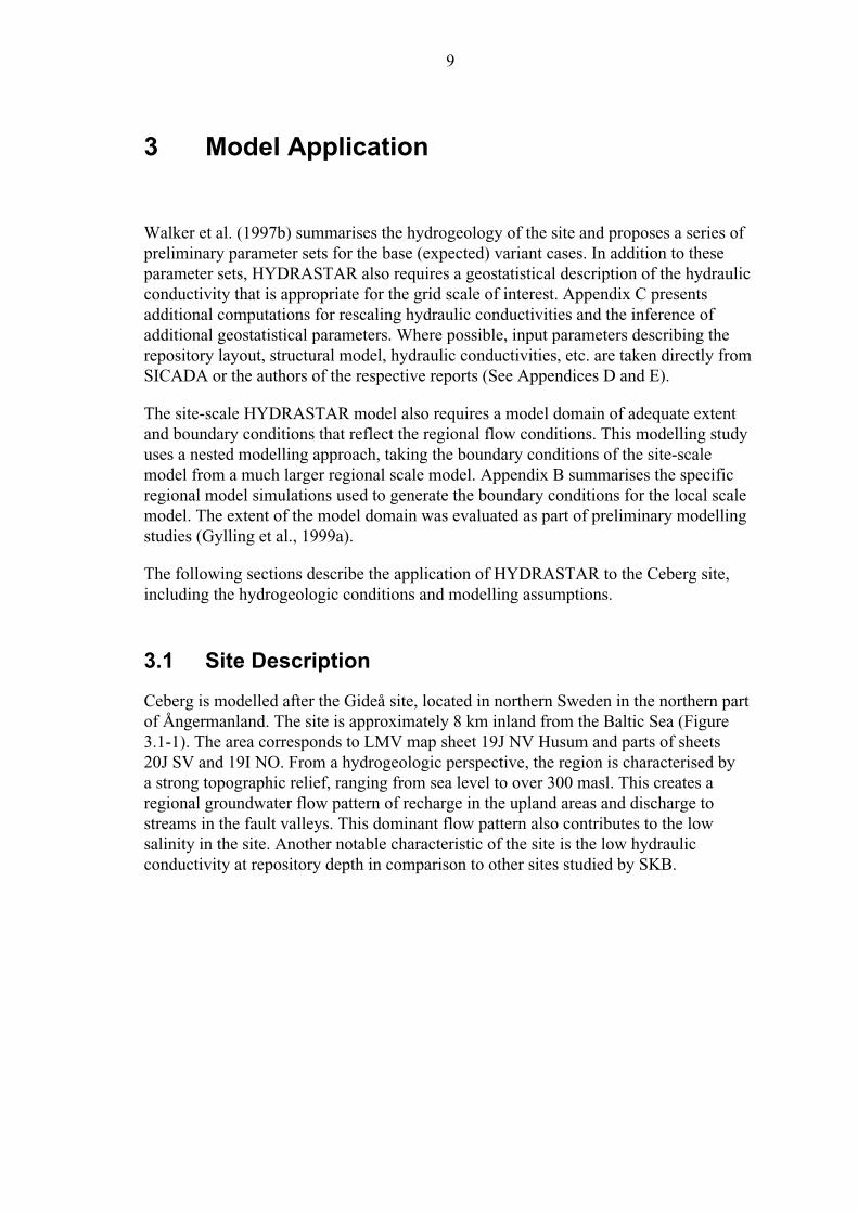
Ceberg is modelled after the Gideå site, located in northern Sweden in the northern part
of Ångermanland. The site is approximately 8 km inland from the Baltic Sea (Figure
3.1-1). The area corresponds to LMV map sheet 19J NV Husum and parts of sheets
20J SV and 19I NO. From a hydrogeologic perspective, the region is characterised by
a strong topographic relief, ranging from sea level to over 300 masl. This creates a
regional groundwater flow pattern of recharge in the upland areas and discharge to
streams in the fault valleys. This dominant flow pattern also contributes to the low
salinity in the site. Another notable characteristic of the site is the low hydraulic
conductivity at repository depth in comparison to other sites studied by SKB.

10
����������������
����������� ���� ������
����������
���������
������
������
���
������
�� �����
����������
�����
����
��
Figure 3.1-1. Location of the Gideå site. Dashed line represents roads.
3.2 Hydrogeology
The geology and hydrogeology of the Gideå site have been studied in detail and aresummarised in a series of reports (Ahlbom et al., 1991; Ahlbom et al., 1983; Hermansonet al., 1997; Askling, 1997; Timje, 1983). Walker et al. (1997b) presents a summary ofsite conditions emphasising continuum modelling.
The bedrock in the Gideå region is migmatised-veined gneiss, dominated by greywackewith subordinate schist, phyllite and slate with varying degrees of metamorphosis.Dolerite intrusive dykes are common in the region and have been observed at the site,typically as subvertical thin dykes with east-west strikes. South of the Gideå site is abody of granite gneiss and to the west is a body of granite (Hermanson et al., 1997).The region continues to experience isostatic rebound as a consequence of the last periodof continental glaciation and exhibits landrise rates amongst the fastest in Sweden,approximately 7.7 mm/yr (Björck and Svensson, 1992). The soil cover is thin generally(less than a metre) with numerous bedrock outcrops, but is somewhat deepert in valleysand larger depressions. Glacial till occurs only sparsely at ground surface, and the soilcover is dominated by marine sediments. Peatlands are found in some depressions, asare wave-washed gravel and sand (Lundqvist et al., 1990).
Regional lineaments have been interpreted from air photos and topographical maps at ascale of 1: 50,000 (Ahlbom et al., 1983; Askling, 1997; Lundqvist et al., 1990). Theselineaments have been interpreted as subvertical fractured zones, striking primarily west-northwest and northwest. In general, however, very little information is available for theregional lineaments, and their inferred characteristics should be regarded as uncertain(Ahlbom et al., 1983; Ericsson and Ronge, 1986; Askling, 1997; Hermanson et al.,

11
1997). On site, a number of steeply dipping fracture zones has been observed, whose
hydraulic conductivity is inferred to be somewhat higher than the surrounding rock
mass.
The groundwater chemistry in the Gideå area is characterised by an overall downward
recharge of precipitation, typical of upland areas with strong topographic drive
(Laaksoharju et al., 1998).
Timje (1983) summarised the Swedish Meteorological and Hydrological Institute
(SMHI) data and constructed a rainfall-runoff model for this region. The resulting
simulations suggest that the mean annual net distributed recharge to the regional
groundwater system is 10 mm, but may vary locally depending on topography. Timje
(1983) constructed a water table map that indicates that the shallow groundwater system
is dominated by recharge on the plateau and discharge to the streams that occupy fault
valleys. The effects of this topographically driven system on the site-scale model are
discussed in the next section.
3.3 Regional Model and Boundary Conditions
The model uses a nested modelling approach, relying on boundary conditions derived
from the regional groundwater flow modelling study of Boghammar et al. (1997; Figure
3.3-1). That study used a finite element continuum model, NAMMU, to study ground
water recharge and regional flow patterns. The results of that study included the steady-
state heads along the limits of the site-scale model domain. Figure 3.3-2 presents the
hydraulic heads estimated by the regional model on the boundaries of the site-scale
model. The smaller regional model of Boghammar et al. (1997) provides the constant
head boundary conditions for the Base Case site-scale model.
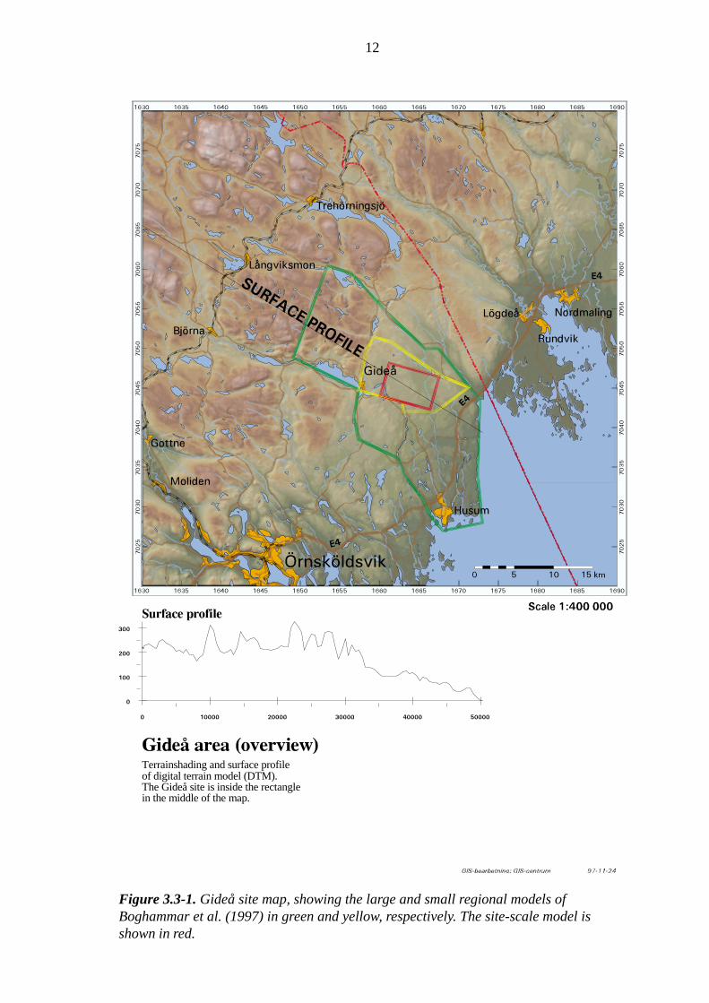
Terrainshading and surface profileof digital terrain model (DTM).The Gideå site is inside the rectanglein the middle of the map.
Figure 3.3-1. Gideå site map, showing the large and small regional models ofBoghammar et al. (1997) in green and yellow, respectively. The site-scale model isshown in red.
12

13
Figure 3.3-2. Constant head boundary conditions for each face of the model domain forCeberg (hydraulic head, in metres).
Bottom
North
West
N
0 1000 m
Approx. Scale
Top East
South

14
Variant 1, with fracture zone conductivities increased by a factor 100, and Variant 2,
with additional fracture zones, require slightly different regional models than the
Base Case to generate appropriate site-scale boundary conditions. For Variant 1, an
appropriate variant from Boghammar et al. (1997) is available to provide the constant
head boundary conditions. For Variant 2, an additional simulation is performed, based
on the regional model of Boghammar et al. (1997; see also Appendix B).
The heads predicted by the regional model along the boundaries of the site-scale model
domain are used as Dirichlet (constant-head) boundary conditions for the site-scale
model. The regional NAMMU model generates the head values using finite element
basis functions to interpolate as necessary between the NAMMU nodes for the
HYDRASTAR grid spacing of 35 m. A HYDRASTAR subroutine reads the inter-
polated heads and uses them as boundary conditions for the HYDRASTAR model
domain. Although this approach is similar to that used in other nested groundwater
models (e.g., Ward et al., 1987; Leake et al., 1998), it is also important to verify that the
flows across the boundaries are the same (i.e., conservation of mass). The consistency of
flow between the regional and site-scale model is discussed further in Section 4.0.
3.4 Model Grid and Repository Layout
The HYDRASTAR model for this application consists of a 3-dimensional finite
difference grid with a uniform grid spacing of 35 m. The regional modelling study of
Boghammar et al. (1997) examined the regional flow pattern to determine a model
domain that would include the majority of exit locations for advective travel paths
starting from the repository. Preliminary simulations by Gylling et al. (1999a) suggested
that a small percentage (approximately 10%) of particles would fail to exit to the upper
model surface and be intercepted by the southern model boundary. This application of
HYDRASTAR uses a domain with an upper surface area of 6510 m by 4290 m,
extending to a depth of 1190 m (Figure 3.4-1). The upper surface of the model is
given 60 masl. The resulting grid of 187×124×35 nodes (width, length and depth,
respectively) gives a relatively large size for HYDRASTAR models that can be run
on the SKB CONVEX.
The performance assessment measures are based on distributions of canister flux, travel
paths and travel times to exit locations in the accessible environment (i.e., ground
surface). Ideally, the model grid upper surface would correspond to the ground surface.
This is not possible in this study because HYDRASTAR uses a flat plane for the upper
model surface. Consequently the observed ground surface is represented as a horisontal
plane with the modelled domain lying below the minimum ground surface elevation
(60 masl). The HYDRASTAR particle tracking algorithm requires a minimum distance
of one grid spacing from any model boundary to calculate the velocity vectors, and thus
the exit location for these simulations is 25 masl. That is, the performance assessment
measures are based on exit locations on a horisontal plane at 25 masl.

15
Figure 3.4-1 also shows the hypothetical repository tunnel layout, a single-level design
specified by Munier et al. (1997, recommended tunnel design). The tunnels of this
repository design lie at an elevation of –500 masl, oriented perpendicular to the
principal regional stress. The design avoids mapped fracture zones, allowing an
exclusion zone whose width depends on the fracture zones’ classification. The tunnels
are placed no closer than 100 m to zones that are classified as certain (e.g., Zone 1), and
no closer than 50 m to those classified as probable (e.g., Zone 7). Note that the tunnel
design does not avoid fracture zones classified as possible, such as the dolerite dykes
(see Section 5.2). This study represents the hypothetical waste canisters with 119
locations uniformly scattered over the repository tunnels (Figure 3.4-2). HYDRASTAR
uses these 119 representative locations as starting positions for the stream tubes and the
subsequent travel time, canister flux and F-ratio calculations.
18x103
16
14
12
10
(RA
K-
7 03
0 00
0) N
orth
->
18x103 16141210
(RAK - 1 650 000) East ->
Husån
Flisbäcken
Västersjön
Skedmarkssjön
Gideån
Åktjärnen
Ceberg
Model boundaries
----- Deposition tunnels
Figure 3.4-1. Gideå site-scale model domain (blue line). Tunnels of the hypotheticalrepository at –500 masl are shown projected to ground surface (scale in metres).

16
14 000
14 500
15 000
15 500
16 000
11 000 11 500 12 000 12 500 13 000 13 500 14 000
East
Nor
th
1
2
3
4
56
7
8
9
10
11
12
13
14
15 16
17
18
19
20
21
22
2324
25
26
2728
29
30
31
32
33
3435
36
37
38
39
40
41
42
43
4445
4647
4849
50
51
52
53
54
55
56
57
58
5960
61
62
63
64
65
66
67
68
69
70
71
72
73
74
75
77
78
79
80
81
82
83
84
85
86
87
88
89
90
9192
9394
95
96
97
98
99
100
101
102
103
104
105106
107
108109
110
111
112
113
114
115116
117
118
119
76
Figure 3.4-2. Ceberg hypothetical repository tunnel layout at –500 masl. Numbered locations are 119 stream tube starting locations asrepresentative canister positions.
16
17
3.5 Input Parameters
HYDRASTAR’s input parameters require a structural, hydraulic and geostatistical
description of the site, all at an appropriate scale. This study uses the site-scale
description based on hydrogeologic information found in Ahlbom et al. (1983),
Timje (1983) and Walker et al. (1997b). The site investigations identified a number of
relatively conductive fracture zones between 5 to 50 m in width. Preliminary reports by
Ahlbom et al. (1983) and Ahlbom et al. (1991) suggested that some fractured zones are
clay-altered with very low hydraulic conductivity, while others are highly conductive.
Thus the assumption that the fracture zones are uniformly conductive features is
uncertain at Ceberg. Fractures elsewhere in the site (i.e., those not included in the
deterministic zones) are collectively included in the hydraulic conductivity estimates
for the rock mass. Consequently, the hydraulic conductivity data are divided into two
populations based on the site structural model (Walker et al., 1997b):
• Rock Domain (RD) – relatively unfractured rocks outside the deterministic
conductors. On the site-scale, this is denoted SRD.
• Conductor Domain (CD) – fractured rocks within the deterministic conductors. On
the site-scale, the set of conductors is collectively referred to as SCD.
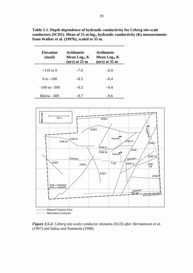
The principal source of hydraulic conductivity data is the injection and pumping tests
performed in the cored boreholes (Figure 3.5-1). These tests were interpreted and the
measurements reported for various depths, rock types, etc. as described by Ahlbom
(1983), Hermanson et al. (1997), and Walker et al. (1997b). The interpreted hydraulic
conductivities for the 25 m packer tests were taken directly from the SKB SICADA
database and analysed with the SKB geostatistical inference code INFERENS.
The scale of these measurements (as inferred from the packer length) is little different
from the proposed model grid scale. However, as discussed in Walker et al. (1997b),
hydraulic conductivity is a scale-dependent parameter, which requires that the measured
hydraulic conductivities be upscaled to the finite difference grid scale of the model. This
study uses the scaling approach described in Appendix C.1. The following sections
present both the geometric means of the test-scale and model-scale hydraulic conduc-
tivities for the conductor domain and the rock domain.

18
����������� ��������
������������� ������ ��������������
�����
����
��
��
��
��
���
�����
�
�� �
��
�����
����� ���
���� ���� ����
�
��
�
�
� � � ��
��
� ��
���
����
����
�����
!����
��
!����" ��# !����# �����#
��
��
�������������������
Figure 3.5-1. Gideå boreholes. Coordinates are a local system used in the KBS-3 study.
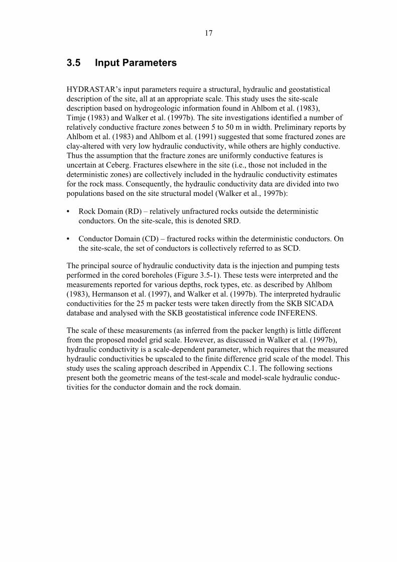
3.5.1 Site-Scale Conductor Domain (SCD)
The geometries of the hydraulic conductor domains on the site-scale (SCD) are definedby the major discontinuities described in Hermanson et al. (1997) and represented asplanar features of constant width (Figure 3.5-2). Unlike Aberg and Beberg, only single-hole borehole tests have been performed at this site, with little additional examination ofthe individual conductive structures. Walker et al. (1997b) inferred a depth-dependantmodel of hydraulic conductivities, dividing the packer test data into a series of stepwisedecreases with depth. Insufficient data are available to infer properties for individualfractures, so the log10 hydraulic conductivity of the fractures is assumed to come froma common distribution whose mean varies with depth. This study assumes that themeasurement scale is 25 m, and correspondingly upscales the reported values to thefinite difference block scale of 35 m using the relationship described in Appendix C.1.Table 3-1 presents the resulting parameter set, denoted SCD1 in Walker et al. (1997b).
19
Table 3-1. Depth dependence of hydraulic conductivity for Ceberg site-scaleconductors (SCD1). Mean of 25 m log10 hydraulic conductivity (K) measurementsfrom Walker et al. (1997b), scaled to 35 m.
Elevation(masl)
ArithmeticMean Log10 K(m/s) at 25 m
ArithmeticMean Log10 K(m/s) at 35 m
+110 to 0 –7.0 –6.9
0 to –100 –8.5 –8.4
–100 to –300 –9.5 –9.4
Below –300 –9.7 –9.6
$% #!
$% #�
$% #!!&
���������� !"#�$#%�������&
$% #!�'#%
$% #'
$% #(
�������(
$% #)
$% #�&$% #��
$% #*
$% #�
$% #�&
$% #��
+����$% #!�
+����
��)*&#++,## ���*(""-###
,�����
.�//���0�� �����1��� �������2������� ���
$% #-
$% #!!��������(
�3����
Figure 3.5-2. Ceberg site-scale conductor domains (SCD) after Hermansson et al.(1997) and Saksa and Nummela (1998).

20
3.5.2 Site-Scale Rock Domain (SRD)
Similar to the conductor domain, the rock domain on the site-scale (SRD) is divided
into elevation zones as given by Walker et al. (1997b). The geometric mean hydraulic
conductivities are based on the interpreted hydraulic conductivities of the 25 m packer
tests. These values must be upscaled from 25 m-measurement scale to 35 m-finite
difference grid scale. Table 3-2 presents the resulting parameter set, denoted SRD6
in Walker et al. (1997b), as the upscaled values used in this study.
Elevation(masl)
ArithmeticMean Log10 K(m/s) at 25 m
ArithmeticMean Log10 K(m/s) 35 m
+110 to 0 –7.6 –7.4
0 to –100 –9.0 –8.9
–100 to –300 –10.0 –9.9
Below –300 –10.3 –10.1
3.5.3 Geostatistical Model
The Ceberg site-scale geostatistical model of hydraulic conductivity consists of depth
zones for SRD6 and SCD1, the structural model of the zones and a single variogram
model. As is discussed in Walker et al. (1997b), the variogram must be adjusted
(regularised) to account for the difference between measurement and grid scales. Note
that only one variogram model can be specified in HYDRASTAR for both domains.
Because the data are most abundant for the rock domain, this study infers a regularised
variogram model based on the upscaled 25 m packer test data in the rock domain SRD
(Walker et al., 1997b). The interpreted conductivities are taken from 13 cored boreholes,
as found in SICADA. The SKB code INFERENS was used to upscale the 25 m data to
50 m and fit a model variogram to the rock mass data (Walker et al., 1997b).
Table 3-2. Depth dependence of hydraulic conductivity for Ceberg site-scalerock mass (SRD6). Mean of 25 m log10 hydraulic conductivity (K) measurementsfrom Walker et al. (1997b), scaled to 35 m.

21
Linear interpolation between the 25 m and 50 m variogram suggests the following
variogram model for the 35 m grid scale (Figure 3.5-3; see also Appendix C.1):
• Exponential model, isotropic,
• practical range of 68 m, and
• zero nugget, log10 K variance of 1.12.
The SRD and SCD are treated as step changes in Kb, the block conductivities (i.e., 0
order trends in log10 Kb), with values provided in Tables 3-1 and 3-2. Figure 3.5-4
shows the representation of the SCD within the model domain, and Figure 3.5-5 is a
deterministic realisation. Figure 3.5-6 is a plot of a single realisation (number 1) of the
log10 K field.
Figure 3.5-3. Semivariograms of log10 hydraulic conductivity for Ceberg rock domain(SRD), for packer test data (25 m), INFERENS-fitted (50 m), and interpolated (35 m).
0.00 200.00 400.00 600.00 800.00Lag Spacing (m)
0.00
0.50
1.00
1.50
Sem
ivar
iogr
am o
f Lo
g K
Res
idua
ls
25 m model
35 m model
50 m model
Ceberg Model Variogram

22
Figure 3.5-4. HYDRASTAR representation of Ceberg conductive fracture zones(SCD1). Coordinates are RAK system offset by 1,650,000 m in east-west and 7,030,000m in north-south (view from above, with RAK North in the y-positive direction, scale inmetres).

23
Figure 3.5-5. Log10 hydraulic conductivity on the upper model surface, Ceberg Variant4 (deterministic representation of hydraulic conductivity, in plan view, with RAK Northin the y-positive direction, scale in metres).

24
Figure 3.5-6. Log10 of hydraulic conductivity for one realisation of Ceberg Base Case.Upper image is plan view, with North in the y-positive direction, scale in metres. Lowerimage is elevation view of the same field, looking North.
3.5.4 Other Parameters
The remaining HYDRASTAR input parameters are hydraulic parameters required for
the transport calculations and performance measures. One of these is the flow (or
kinematic) porosity, εf, which is not easily characterised under the best of conditions.
Based on analogue data at Äspö (Rhén et al., 1997), this study uses a flow porosity of
εf = 1×10⁻⁴
, uniform over the entire domain. It should be noted that the travel times
reported in this study are directly proportional to this assumed flow porosity.

25
Another hard-to-define parameter is ar, the flow-wetted surface area per rock volume.
Similar to the flow porosity, the flow-wetted surface is assumed to be uniform over
the entire model. For Ceberg, Andersson (1999) report a range of 1.0 to 0.01 and
recommend the value ar = 0.1 m2/(m
3 rock) as the best estimate. This parameter is
not used directly as model input for HYDRASTAR, but it is used in calculating the
F-ratio, defined as:
f
rw
w
rw at
q
adF
ε==
Where:
dw = travel distance for a particle [metres]
qw = Darcy velocity = v•εf [metres/year]
ar = specific surface per rock volume for a travel path [m2/(m
3 rock)]
εf = flow (kinematic) porosity [ . ]
The F-ratio [years / m] is a ratio of resisting to driving forces for transport, which has
been used to compare model results in performance assessments (SKI, 1997). The
F-ratio is useful in evaluating repository performance in the case of sorbing nuclides,
where the transit time depends on both the surface area available for sorption and on the
Darcy velocity. Although the F-ratio is calculated for all cases, it is a simple multiple of
the travel time and is therefore plotted only for the Base Case. SR 97 uses the F-ratio to
compare the geosphere performance for the three hypothetical repositories, where the
flow-wetted surface varies from site to site.

27
4 Base Case
This section of the report presents the simulation and analysis for the Base Case, which
represents the expected site conditions as described in Section 3, and it is the reference
case for comparison to all other cases. A premodelling study by Gylling et al. (1999a)
examined the extent of the domain and suggested a volume likely to contain all exit
locations. Boundaries for this domain are specified head (Dirichlet) boundaries on all
sides of the model domain, taken from the steady-state head values of a deterministic,
freshwater simulation with the regional model of Boghammar et al (1997, case GRST).
Mapped fracture zones are modelled as conductive features and included as determin-
istic conductor domains (SCD). The site-scale hydraulic conductivity field is created
with an unconditional simulation (i.e., no direct use of measured hydraulic conductivi-
ties), prescribing the mean of log10 hydraulic conductivity for each rock unit.
One hundred realisations of the hydraulic conductivity field, each with 119 starting
locations, are used to estimate the distributions of travel time and canister fluxes. All
statistics are calculated with respect to the common logarithm transforms (log10 ) to
facilitate summary and display. No formal test for the lognormality of these results has
been performed or is inferred.
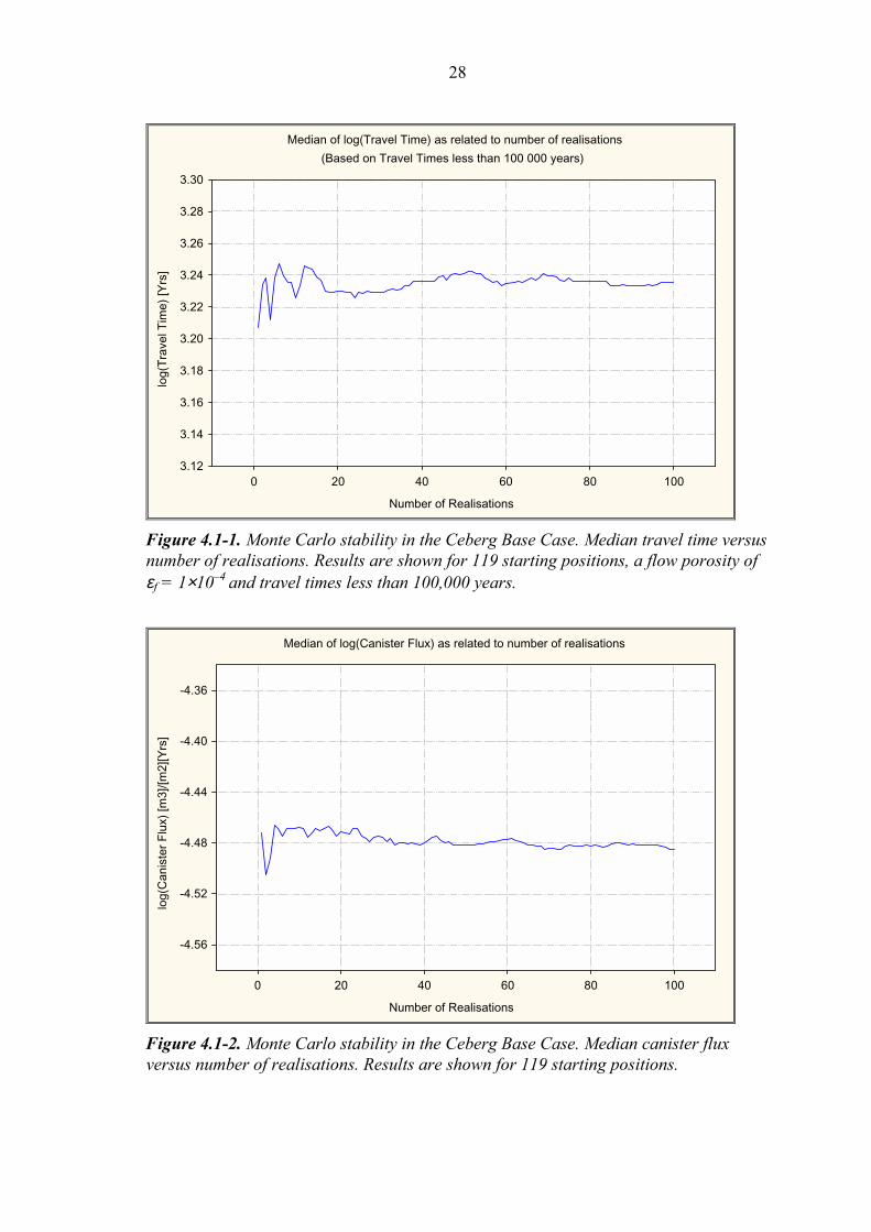
4.1 Monte Carlo Stability
A practical consideration in Monte Carlo simulation studies is that statistics of interest
be stable with respect to the number of realisations. That is, the number of realisations
should be adequate for reliable estimates of the results. This study monitored the
stability of the estimators of the median travel time and median canister fluxes with
respect to the number of realisations. Figures 4.1-1 and 4.1-2 present the medians of
the logarithm of travel time and the logarithm of canister flux, respectively, versus the
number of realisations. The plots indicate these statistics are approximately constant
after 30 realisations, with less than 3% deviation for additional realisations. Thus, for
the purposes of this study, a total number of 100 realisations were performed.
The stability of the sample median and arithmetic mean should not be taken to imply
that higher moments such as the sample variance are also stable. Estimators of higher
moments and the extreme quantiles of distributions are usually much less efficient than
the median or the mean (Larsen and Marx, 1986). In general, estimating these moments
with a similar degree of accuracy requires many more realisations than are needed for
stable estimators of the median (Hammersley and Handscomb, 1975). Consequently,
the higher-order statistics may not have stabilised and should be used cautiously.
28
Median of log(Travel Time) as related to number of realisations
(Based on Travel Times less than 100 000 years)
Number of Realisations
log(
Tra
vel T
ime)
[Yrs
]
3.12
3.14
3.16
3.18
3.20
3.22
3.24
3.26
3.28
3.30
0 20 40 60 80 100
Figure 4.1-1. Monte Carlo stability in the Ceberg Base Case. Median travel time versusnumber of realisations. Results are shown for 119 starting positions, a flow porosity ofεf = 1×10⁻⁴ and travel times less than 100,000 years.
Median of log(Canister Flux) as related to number of realisations
Number of Realisations
log(
Can
iste
r F
lux)
[m3]
/[m2]
[Yrs
]
-4.56
-4.52
-4.48
-4.44
-4.40
-4.36
0 20 40 60 80 100
Figure 4.1-2. Monte Carlo stability in the Ceberg Base Case. Median canister fluxversus number of realisations. Results are shown for 119 starting positions.

29
4.2 Boundary Flux Consistency
Stochastic continuum theory suggests that, under certain conditions, there is an effective
hydraulic conductivity, Ke, which satisfies:
hKq e
vv ∇−=
Where:
qv
= the expected flux
hv
∇ = the expected gradient
Ke is useful for nested models in that it can be used to estimate the expected value of
the flux in a smaller domain (Dagan, 1986; Rubin and Gómez-Hernández, 1990). This
suggests that a regional model with a homogeneous hydraulic conductivity of Ke could
be used to determine the expected boundary fluxes of a site-scale model. If the rescaling
of the geometric mean hydraulic conductivity is correct, the boundary flux of the
regional model should be consistent with the average boundary flux of the site-scale
stochastic continuum model. That is, the site-scale stochastic continuum model should
conserve mass in an average sense with respect to the regional model fluxes.
Walker et al. (1997) suggested that the upscaling of block scale hydraulic conductivity
could be calibrated using this relationship, adjusting the mean block hydraulic con-
ductivity until the boundary fluxes of the ensemble matched the regional scale fluxes.
However, there are several drawbacks to that approach. For example, the existence of Ke
requires that the domain be stationary, extensive and under uniform flow conditions. In
addition, the regional models conserve mass over the entire domain in an average sense,
but may not conserve mass over arbitrary subdomains. Because of these limitations, this
study does not adjust the mean block hydraulic conductivity to improve the flow balance
between the models. However, as a check on the nested modelling and the upscaling of
hydraulic conductivity, this study calculates the net volumetric flow of water across the
boundaries. These flows are also reported as a mass balance for the regional and site
models individually as a check on model internal consistency.
As shown in Figure 4.2-1, both models indicate that the majority of the inflow to the
domain comes from surface recharge, and the majority of the outflow occurs across the
southern model boundary. These flows represent the net flow across a boundary, and
consequently do not reflect the complex distribution of inflows and outflows on each of
the surfaces. The top surface, for example, has a net recharge due to precipitation, but
also discharges to the mires and streams near the site. Table 4-1 summarises the flow for
each face of the model domain. Note that the site-scale mass balance calculations carry
only three significant digits, and thus contribute some error (Lovius, 1998).

30
4
�5�����6
)5����6
������ �����7�������������8�9� �7/�������:)(#��7�;�<
Σ=�≈ ->##5Σ=�≈ �#>##(+6
5�/6
->,$5#>-'$6
(">&5#>$-#6
#>##-&$5�#>#--(6
(&>&5#>,,&6 �>'+
5#>#$$,6
->-,5#>(,#6
Figure 4.2-1. Consistency of Ceberg boundary flow, regional versus site-scale models.The arithmetic mean flow for five realisations of the site-scale model is shown inparentheses. Arrows denote the regional flow direction.
Table 4-1. Boundary flow consistency for Ceberg Base Case, regional model ofBoghammar et al. (1997) versus site-scale.
Net Flow Through Site Model Surfaces (m3/s × 10–3)
Model Surface Regional Base Case(GRST)
Site-scale Base Case (5 realisations)
West 2.59 (in) 0.289 (in)East 2.25 (in) 0.150 (in)South 16.7 (out) 0.920 (out)North 3.84 (out) 0.0995 (out)Bottom 0.00279 (out) 0.0221 (in)Top 17.7 (in) 0.557 (in)Total Inflow 22.54 1.02Total Outflow 20.54 1.02Mass balance (In – Out) 2.00 –0.001
31
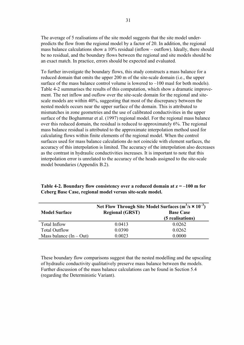
The average of 5 realisations of the site model suggests that the site model under-
predicts the flow from the regional model by a factor of 20. In addition, the regional
mass balance calculations show a 10% residual (inflow – outflow). Ideally, there should
be no residual, and the boundary flows between the regional and site models should be
an exact match. In practice, errors should be expected and evaluated.
To further investigate the boundary flows, this study constructs a mass balance for a
reduced domain that omits the upper 200 m of the site-scale domain (i.e., the upper
surface of the mass balance control volume is lowered to –100 masl for both models).
Table 4-2 summarises the results of this computation, which show a dramatic improve-
ment. The net inflow and ouflow over the site-scale domain for the regional and site-
scale models are within 40%, suggesting that most of the discrepancy between the
nested models occurs near the upper surface of the domain. This is attributed to
mismatches in zone geometries and the use of calibrated conductivities in the upper
surface of the Boghammar et al. (1997) regional model. For the regional mass balance
over this reduced domain, the residual is reduced to approximately 6%. The regional
mass balance residual is attributed to the approximate interpolation method used for
calculating flows within finite elements of the regional model. When the control
surfaces used for mass balance calculations do not coincide with element surfaces, the
accuracy of this interpolation is limited. The accuracy of the interpolation also decreases
as the contrast in hydraulic conductivities increases. It is important to note that this
interpolation error is unrelated to the accuracy of the heads assigned to the site-scale
model boundaries (Appendix B.2).
Table 4-2. Boundary flow consistency over a reduced domain at z = –100 m forCeberg Base Case, regional model versus site-scale model.
Net Flow Through Site Model Surfaces (m3/s ×× 10–3)Model Surface Regional (GRST) Base Case
(5 realisations)Total Inflow 0.0413 0.0262
Total Outflow 0.0390 0.0262
Mass balance (In – Out) 0.0023 0.0000
These boundary flow comparisons suggest that the nested modelling and the upscaling
of hydraulic conductivity qualitatively preserve mass balance between the models.
Further discussion of the mass balance calculations can be found in Section 5.4
(regarding the Deterministic Variant).

32
4.3 Ensemble Results
4.3.1 Travel Time and F-ratio
In each realisation, HYDRASTAR calculates the travel times for a particle to be
advected from each starting position (release position) to the model surface. The
resulting stream tubes are used later in one-dimensional transport calculations in the
PA model chain. Although the advective travel time is a common statistic for comparing
variant simulations, it is important to note that HYDRASTAR allows only a homo-
genous flow porosity to be specified for the entire domain. Consequently, the travel
time in any stream tube is directly proportional to this homogeneous flow porosity. This
study simply uses the flow porosity of εf = 1×10⁻⁴
, and leaves further analysis of the
flow porosity to the transport modelling studies associated with SR 97.
Figure 4.3-1 presents the frequency histogram for the common logarithm of travel time
for 100 realisations, each with 119 starting positions. A series of outliers are seen at
the extreme upper tail of the histogram, corresponding to travel times of 100,000 years.
These are the travel times for stream tubes that are intercepted by the southern, eastern
and bottom surfaces of the model and that fail to exit the model’s upper surface
(approximately 10% of the total number of stream tubes; see Figure 4.4-1). In this
circumstance, HYDRASTAR sets the travel times for these stream tubes to the default
maximum travel time of 100,000 years.
The use of the default travel time does have noticeable effects on the performance
measure statistics, as shown in Table 4-3 for the Base Case. To quantify this effect, this
study calculates the statistics both with and without the travel times greater than 100,000
years. The means and variances of the travel time and F-ratio change slightly if stream
tubes with the default travel time of 100,000 years are deleted. In contrast, the canister
flux statistics are virtually unaffected by this censoring, as are the medians of travel time
and F-ratio. For the remainder of this study, the performance measure statistics are
calculated both with and without the travel times greater than 100,000 years. For the
sake of brevity, the discussions will emphasise the medians of all measures and the
statistics of travel time and F-ratio for travel times less than 100,000 years. The canister
flux will be summarised with statistics computed for the full set of stream tubes (no
deletions). The variances and medians of the performance measures are emphasised in
bold in the summary tables (e.g., Table 4-3). The effects of this censoring on subsequent
performance assessment calculations are beyond the scope of this study.

33
Histogram of log(Travel Time) : 100 realizations
log(Travel Time) [Yrs]
Fra
ctio
n
0.00
0.04
0.08
0.12
0.16
0.20
0.24
0.28
-2.0 -1.5 -1.0 -0.5 0.0 0.5 1.0 1.5 2.0 2.5 3.0 3.5 4.0 4.5 5.0 5.5 6.0
Figure 4.3-1. Relative frequency histogram of log10 travel time for Ceberg Base Case.Results are shown for 100 realisations of 119 starting positions and a flow porosity ofεf = 1×10⁻⁴.
Table 4.3 summarises the ensemble results, presenting the statistics for the 100 Monte
Carlo realisations of all 119 starting positions for travel time, canister flux and F-ratio.
With the intercepted stream tubes deleted, the median travel time is 1720 years, with an
interquartile range from 953 to 2965 years and a variance of log10 travel time of 0.123.
Exclusive of the outliers, the distribution is almost perfectly symmetric. Figure 4.3-2
presents a box plot of the travel times by realisation, which indicates that the range of
travel times in any single realisation can be extreme, ranging from a 5th
percentile of
436 years to a 95th
percentile of 6152 years.

34
25%, 75%5%, 95%Median
Box plot of log(Travel Time)
Realization Number
log(
Tra
vel T
ime)
[Yrs
]
2.0
2.4
2.8
3.2
3.6
4.0
4.4
4.8
5.2
0 20 40 60 80 100
Figure 4.3-2. Travel times by realisation for Ceberg Base Case. Results are shown for119 starting positions and a flow porosity of εf = 1×10⁻⁴.
All values Travel Times > 100,000 yearsdeleted
Log10
tw
Log10 qc Log10 F-ratio
Log10 tw Log10 qc Log10 F-ratio
Mean 3.407 –4.499 6.407 3.224 –4.501 6.224
Median 3.288 –4.485 6.288 3.236 –4.488 6.236Variance 0.401 0.182 0.401 0.123 0.182 0.1235
th percentile 2.654 –5.220 5.654 2.639 –5.225 5.639
25th
percentile 3.011 –4.781 6.011 2.979 –4.785 5.979
75th
percentile 3.572 –4.204 6.572 3.472 –4.205 6.472
95th
percentile 5.000 –3.814 8.000 3.789 –3.815 6.789
Table 4-3. Summary statistics for Ceberg Base Case. Results are shownfor 100 realisations of 119 starting positions, a flow porosity of εεf = 1××10–4
and flow-wetted surface ar = 0.1 m2/(m3 rock). Statistics in bold arediscussed in the text. Approximately 10% of the stream tubes fail to reachthe upper surface.

35
Number of Realisations versus the Stream Tube Number with:
log(Travel Time) less than 1000 years (squares)
log(Travel Time) less than 100000 years (bars)
Stream Tube Number
Num
ber
of R
ealis
atio
ns
0
20
40
60
80
100
120
-20 0 20 40 60 80 100 120 140
Figure 4.3-3. Number of realisations with travel times less than 1000 years (squares)and 100,000 years (lines), by stream tube number for Ceberg Base Case. Results areshown for 100 realisations of 119 starting positions and a flow porosity of εf = 1×10⁻⁴.
Figure 4.3-3 presents a box plot of the number of realisations with travel times less
than a certain cut-off time, by stream tube (starting position number). There are several
patterns that can be observed in this plot, for example the cycle of increasing travel time
for certain sequences of starting position numbers (e.g., from location 11 to location 32).
This pattern is an artefact of the numbering sequence of the stream tube starting posi-
tions, where the sequence of starting position numbers corresponds to a line running SW
to NE in the repository. The SW side of the repository is relatively close to an important
exit area, and the NE side of the repository is upgradient. Because the starting position
numbers follow a sequence roughly parallel to the gradient in the central part of the
repository (Figure 3.4-2), the sequence of starting position numbers 11 to 32 corre-
sponds to an increase in travel path length. The other pattern that can be observed in
Figure 4.3-3 is the reduced total number of realisations for some stream tubes with
starting position numbers between 99 to 119. These stream tubes frequently are inter-
cepted by the lateral boundaries of the model domain, and are consequently assigned
the default maximum travel time (100,000 years). Stream tubes with starting position
numbers between 90 to 98 are intercepted by the bottom surface of the model domain,
and are likewise assigned the default maximum travel time.
The median F-ratio is 1.72×10⁶ year/m with an interquartile range from 9.53×10
5 to
2.97×10⁶ year/m and a variance of log10 F-ratio of 0.123 (the same as the variance of
log10 travel time; Table 4-3). Figure 4.3-4 presents the frequency histogram for the
common logarithm of the F-ratio for 100 realisations, each with 119 starting positions

36
for travel times less than 100,000 years. This histogram is essentially identical to the
histogram of log10 travel times (Figure 4.3-1) because the F-ratio is a simple multiple of
the travel time (see Section 3.5.4). This report presents the F-ratio for all variants, but in
the interest of brevity will present the histogram of F-ratio only for the Base Case.
Histogram of log(F-factor) : 100 realizations
(Based on Travel Times less than 100 000 years)
log(F-factor)
Fra
ctio
n
0.00
0.06
0.12
0.18
0.24
0.30
3.0 4.5 6.0 7.5 9.0
Figure 4.3-4. Relative frequency histogram of log10 F-ratio for Ceberg Base Case. Results are shown for 100 realisations of 119 starting positions, a flow porosity ofεf = 1×10⁻⁴ and a flow-wetted surface of ar = 0.1 m2/(m3 rock).
4.3.2 Canister Flux
HYDRASTAR calculated the canister fluxes (Darcy groundwater velocity) at each of
the 119 starting positions. Table 4-3 summarises the results for the canister flux, which
indicate a median canister flux of 3.27×10⁻⁵
m/year with an interquartile range from
1.66×10⁻⁵
to 6.25×10⁻⁵
m/year and a log10 canister flux variance of 0.182. Figure 4.3-5
presents the frequency histogram for log10 canister for the ensemble of 100 realisations.
The distribution is nearly symmetric, reflecting the single mean and variance of the rock
domain (i.e., there is no obvious mixing of populations resulting in a bimodal or skewed
distribution). Figure 4.3-6 presents a box plot of log10 canister flux, which indicates no
obvious pattern in the canister fluxes and that the values range over 1.5 orders of
magnitude. Figure 4.3-7 presents a plot of log10 travel times vs. log10 canister flux,
indicating that they have a weak inverse correlation. This might not be true for
models with a stronger correlation structure or greater contrast between RD and
CD conductivities. This is discussed further in Section 5.2.

37
Histogram of log(Canister Flux) : 100 realizations
log(Canister Flux) [m3]/[m2][Yrs]
Fra
ctio
n
0.00
0.05
0.10
0.15
0.20
0.25
0.30
0.35
-8.0 -7.5 -7.0 -6.5 -6.0 -5.5 -5.0 -4.5 -4.0 -3.5 -3.0 -2.5 -2.0 -1.5 -1.0 -0.5 0.0 0.5 1.0 1.5 2.0
Figure 4.3-5. Relative frequency histogram of log10 canister flux for Ceberg Base Case.Results are shown for 100 realisations of 119 starting positions.
25%, 75%5%, 95%Median
Box plot of log(Canister Flux)
Realization Number
log(
Can
iste
r F
lux)
[m3]
/[m2]
[Yrs
]
-5.6
-5.2
-4.8
-4.4
-4.0
-3.6
0 20 40 60 80 100
Figure 4.3-6. Box plot of log10 canister flux for Ceberg Base Case, by realisation.Results are shown for 119 starting positions.

38
Plot of log(Travel Time) versus log(Canister Flux) : 100 realizations
log(Canister Flux) [m3]/[m2][Yrs]
log(
Tra
vel T
ime)
[Yrs
]
Dat
a F
ile N
ame:
cba
s.ni
m
-2
-1
0
1
2
3
4
5
6
-8 -7 -6 -5 -4 -3 -2 -1 0 1 2
Figure 4.3-7. Log10 travel time versus log10 canister flux for Ceberg Base Case.Results are shown for 100 realisations of 119 starting positions and a flow porosityof εf = 1×10⁻⁴.
4.3.3 Flow Pattern and Exit Locations
The regional groundwater flow pattern is one of precipitation recharge on upland areas,
discharging to streams and mires in lowlands (Sections 3 and 4.2). This flow pattern is
reflected in the pattern of stream tubes calculated by HYDRASTAR, as shown in Figure
4.3-8. The stream tubes are directed predominantly downward, then radiating outward to
discharge areas in to the east and southwest. The major discharge areas are the mires to
the southwest of the repository (Tremyrorna, Högmyrån) and the mires and stream to the
east of the repository (Husån).
As discussed in Section 3, the mapped fracture zones have a low hydraulic conductivity
compared to fracture zones at other SKB sites. In addition, the spatial correlation is
short relative to the block length, so that the conductive features representing the
fracture zones will have little continuity. Thus we should expect the fracture zones
as represented in the model to have relatively little influence on the stream tubes.
Figure 4.3-8 also shows the stream tubes for a single realisation relative to the CD. The
stream tubes are diverted by the fracture zones, but in many instances stream tubes pass
directly through the fracture zones.
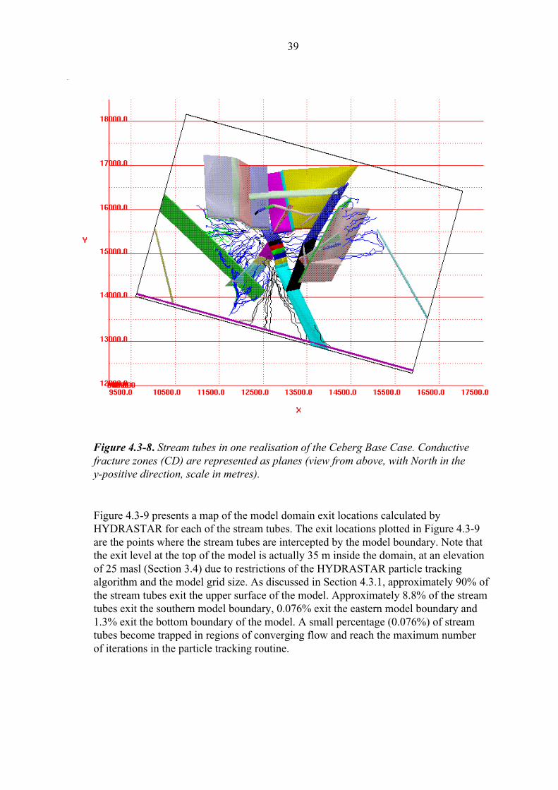
39
Figure 4.3-8. Stream tubes in one realisation of the Ceberg Base Case. Conductivefracture zones (CD) are represented as planes (view from above, with North in they-positive direction, scale in metres).
Figure 4.3-9 presents a map of the model domain exit locations calculated by
HYDRASTAR for each of the stream tubes. The exit locations plotted in Figure 4.3-9
are the points where the stream tubes are intercepted by the model boundary. Note that
the exit level at the top of the model is actually 35 m inside the domain, at an elevation
of 25 masl (Section 3.4) due to restrictions of the HYDRASTAR particle tracking
algorithm and the model grid size. As discussed in Section 4.3.1, approximately 90% of
the stream tubes exit the upper surface of the model. Approximately 8.8% of the stream
tubes exit the southern model boundary, 0.076% exit the eastern model boundary and
1.3% exit the bottom boundary of the model. A small percentage (0.076%) of stream
tubes become trapped in regions of converging flow and reach the maximum number
of iterations in the particle tracking routine.
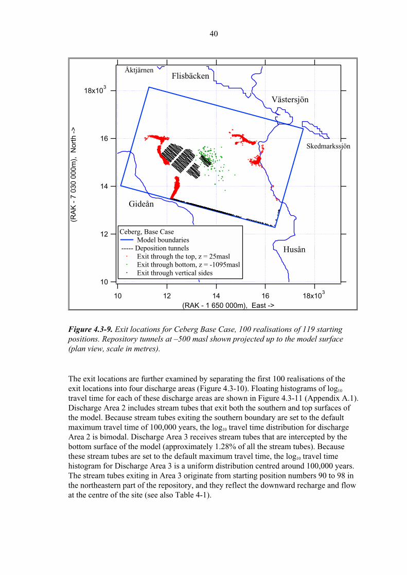
40
Figure 4.3-9. Exit locations for Ceberg Base Case, 100 realisations of 119 startingpositions. Repository tunnels at –500 masl shown projected up to the model surface(plan view, scale in metres).
The exit locations are further examined by separating the first 100 realisations of the
exit locations into four discharge areas (Figure 4.3-10). Floating histograms of log10
travel time for each of these discharge areas are shown in Figure 4.3-11 (Appendix A.1).
Discharge Area 2 includes stream tubes that exit both the southern and top surfaces of
the model. Because stream tubes exiting the southern boundary are set to the default
maximum travel time of 100,000 years, the log10 travel time distribution for discharge
Area 2 is bimodal. Discharge Area 3 receives stream tubes that are intercepted by the
bottom surface of the model (approximately 1.28% of all the stream tubes). Because
these stream tubes are set to the default maximum travel time, the log10 travel time
histogram for Discharge Area 3 is a uniform distribution centred around 100,000 years.
The stream tubes exiting in Area 3 originate from starting position numbers 90 to 98 in
the northeastern part of the repository, and they reflect the downward recharge and flow
at the centre of the site (see also Table 4-1).
18x103
16
14
12
10
(RA
K -
7 0
30 0
00m
), N
orth
->
18x103 16141210
(RAK - 1 650 000m), East ->
Husån
Flisbäcken
Västersjön
Skedmarkssjön
Gideån
Åktjärnen
Ceberg, Base Case
Model boundaries
----- Deposition tunnels
Exit through the top, z = 25masl
Exit through bottom, z = -1095masl
Exit through vertical sides

41
18x103
16
14
12
10
Nor
th -
>
18x103 16141210
East ->
Husån
Flisbäcken
Västersjön
Skedmarkssjön
Gideån
Åktjärnen
Area 1
Area 2
Area 3
Area 4
Figure 4.3-10. Discharge areas and exit locations for the Ceberg Base Case. Resultsare shown for 100 realisations of 119 starting positions (plan view, scale in metres).
Area 1Area 2Area 3Area 4
Floating histograms of log(Travel Time) for different End Point Areas: 100 real
log(Travel Time) [Yrs]
Fra
ctio
n
0.0
0.1
0.2
0.3
0.4
-2 -1 0 1 2 3 4 5 6
Figure 4.3-11. Floating histogram of log10 travel time for stream tubes exiting to thedischarge areas shown in Figure 4.3-10. Results are shown for 100 realisations of 119
starting positions and a flow porosity of εf = 1×10⁻⁴.

42
As discussed above, HYDRASTAR does not explicitly report the travel times for
stream tubes that are intercepted by the side and bottom boundaries of the model. In this
circumstance, HYDRASTAR sets the travel time to the default maximum of 100,000
years. It is possible to post-process the stream tube output of HYDRASTAR using
MatLab scripts to determine the exit locations and the travel time to the southern
boundary. Figure 4.3-12 presents the exit locations on the southern boundary. Although
there is a linear pattern suggesting that a fracture zone is controlling the flow pattern,
this is exclusively the effect of the regional flow pattern. The median travel time of the
stream tubes intercepted by this boundary is 5082 years, with an interquartile range from
3758 to 7145 years. For the stream tubes intercepted by the bottom boundary of the site,
the median travel time is 4055 years, with an interquartile range from 2655 to 5888
years.
Figure 4.3-12. Exit locations on the southern model surface for the Ceberg Base Case.Results are shown for 100 realisations of 119 starting positions (elevation view lookingNorth, scale in metres).
4.3.4 Validity of Results
An approximate calculation of the travel time was performed as a check on the validity
of the model. These computations used Darcy’s Law, the estimated gradient, a simple
flow path, and the mean hydraulic conductivities to estimate the advective travel time
from the centre of the repository to the exit locations to the south and east of the site
(Appendix C.2). The results showed that the travel time should be on the order of 1000
years, roughly in agreement with the median travel time of the Base Case.
In a previous modelling study of the Gideå site, Carlsson et al. (1983) determined the
advective travel times from –500 depth to ground surface. Using a flow porosity of
εf = 4×10
–3, they found that the travel times ranged from 1000 to 300,000 years.
Although the range of their results is extreme, the results of the Carlsson et al. study
suggest that the travel times of this study are reasonable.
-1200
-1000
-800
-600
-400
-200
0
Dep
th [m
]
17x103 16151413121110
East ->
Ceberg Base Case, 981201 Model boundaries Exit through southern side

43
It is also useful to compare the observed heads from boreholes at Gideå site versus the
simulated heads. Although a limited amount of head data are available, it is from a
relatively short monitoring interval and is therefore not believed to be representative
of the long-term steady-state conditions represented by the Base Case (Ahlbom et al.,
1991). Consequently, this study does not directly compare model-simulated heads
versus observed heads.
4.4 Individual Realisations
There are several strategies that could be used to select several realisations that are in
some sense representative of the ensemble. For example, we could select a realisation
whose travel time or canister flux is close to the median of the ensemble of the
realisations. However, the probability of each realisation in a Monte Carlo set is
equal by definition, so that no single realisation can be said to be representative of the
ensemble. This study examines three random realisations to illustrate the variability in
and among individual realisations.
Figure 4.4-1 presents the stream tubes in realisation number one of the Base Case. The
stream tubes reflect the overall downward and lateral flow pattern at the site, as a result
of the regional flow pattern.
As an illustration of the variability within and between realisations, the first three
realisations of the Base Case are examined in more detail (note that these realisations
are randomised by the random number generation). Figure 4.4-2 presents plan views of
the stream tubes for the first three realisations of the Base Case. Although the general
flow pattern remains the same from realisation to realisation, the exit locations can vary
widely for any particular stream tube.
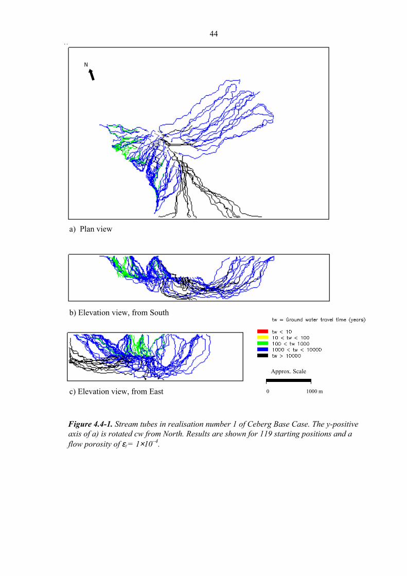
44
Figure 4.4-1. Stream tubes in realisation number 1 of Ceberg Base Case. The y-positiveaxis of a) is rotated cw from North. Results are shown for 119 starting positions and aflow porosity of εf = 1×10⁻⁴.
a) Plan view
b) Elevation view, from South
Approx. Scale
N
a) Plan view
c) Elevation view, from East 0 1000 m
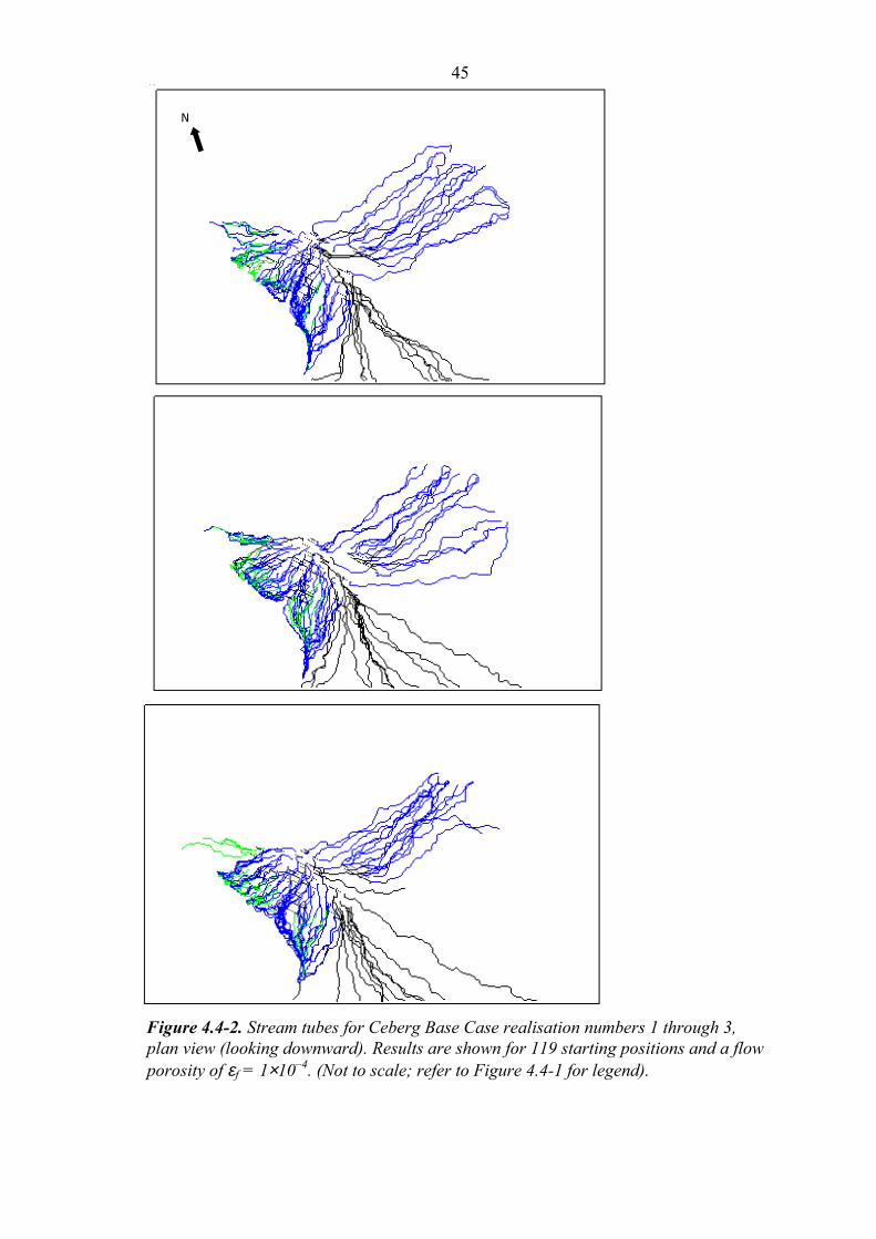
45
Figure 4.4-2. Stream tubes for Ceberg Base Case realisation numbers 1 through 3,plan view (looking downward). Results are shown for 119 starting positions and a flowporosity of εf = 1×10⁻⁴. (Not to scale; refer to Figure 4.4-1 for legend).
N

46
Table 4.4 presents the summary statistics for the realisations shown in Figure 4.4-2. The
statistics suggest that the variances of log10 travel time and log10 canister flux are rather
high within a realisation. In contrast, the medians of these performance measures change
very little from one realisation to the next. This suggests that the variability of perfor-
mance measures is the result of spatial variability within a realisation, and not the
variability between realisations. This suggestion is confirmed by the floating histograms
of these performance measures, which show little difference in shape or location from
realisation to realisation (Figure 4.4-3; Appendix A.1).
Within each realisation, the travel time and canister flux can vary widely. Figures 4.4-4
and 4.4-5 present plots of travel time and canister flux, respectively, versus starting
position number. Although the canister fluxes show no specific pattern (Figure 4.4-5),
the travel times show a cyclical pattern that reflects the travel path length (Figure 4.4-4;
see also Section 4.3.1).
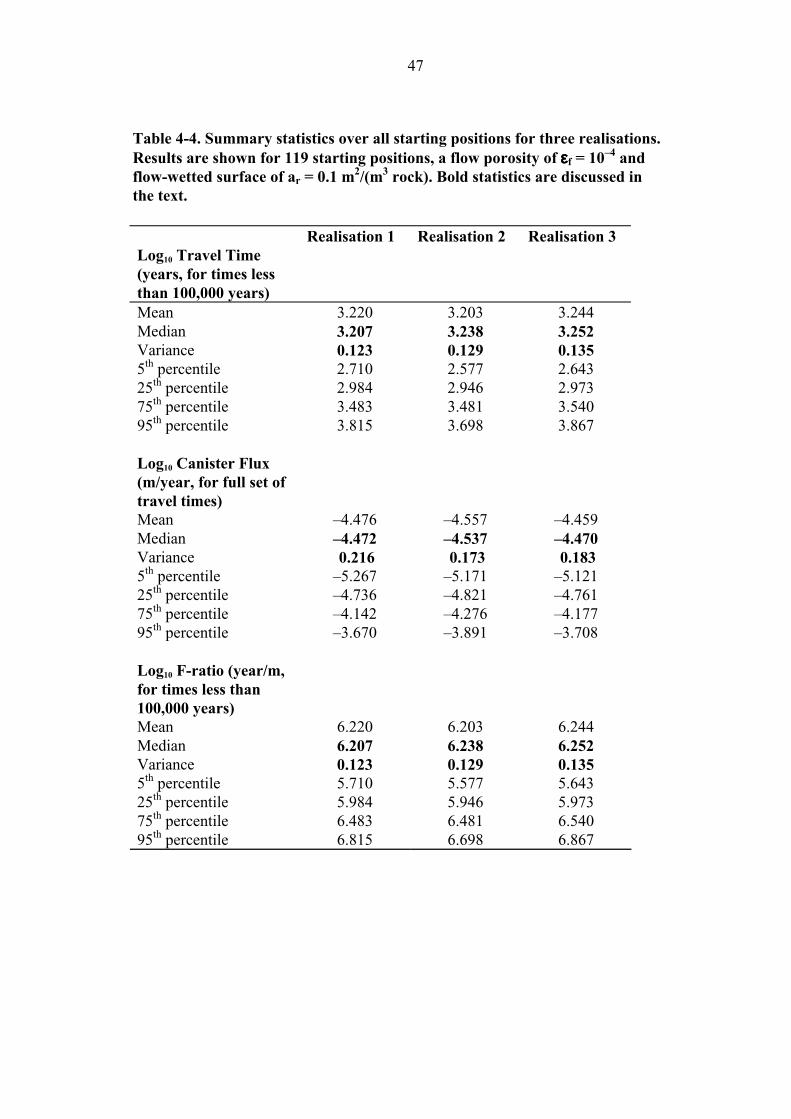
47
Table 4-4. Summary statistics over all starting positions for three realisations. Results are shown for 119 starting positions, a flow porosity of εεf = 10–4 andflow-wetted surface of ar = 0.1 m2/(m3 rock). Bold statistics are discussed inthe text.
Realisation 1 Realisation 2 Realisation 3Log10 Travel Time(years, for times lessthan 100,000 years)Mean 3.220 3.203 3.244
Median 3.207 3.238 3.252Variance 0.123 0.129 0.1355
th percentile 2.710 2.577 2.643
25th
percentile 2.984 2.946 2.973
75th
percentile 3.483 3.481 3.540
95th
percentile 3.815 3.698 3.867
Log10 Canister Flux(m/year, for full set oftravel times)Mean –4.476 –4.557 –4.459
Median –4.472 –4.537 –4.470Variance 0.216 0.173 0.1835
th percentile –5.267 –5.171 –5.121
25th
percentile –4.736 –4.821 –4.761
75th
percentile –4.142 –4.276 –4.177
95th
percentile –3.670 –3.891 –3.708
Log10 F-ratio (year/m,for times less than100,000 years)Mean 6.220 6.203 6.244
Median 6.207 6.238 6.252Variance 0.123 0.129 0.1355
th percentile 5.710 5.577 5.643
25th
percentile 5.984 5.946 5.973
75th
percentile 6.483 6.481 6.540
95th
percentile 6.815 6.698 6.867
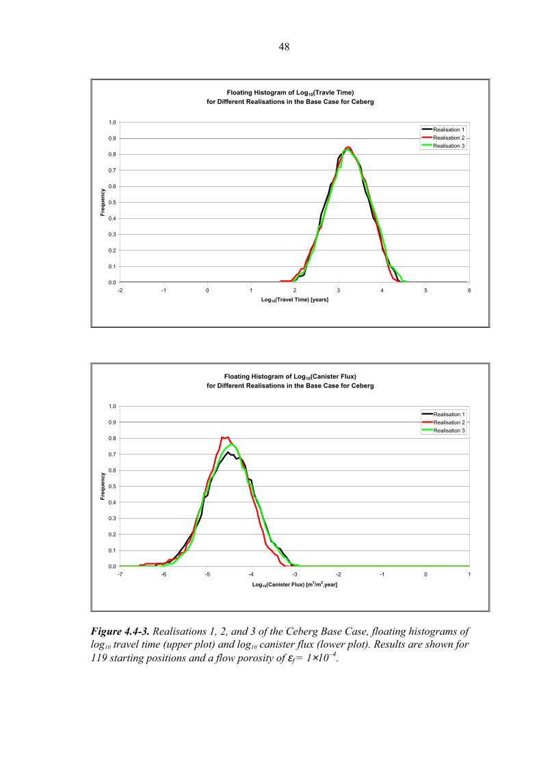
48
Floating Histogram of Log10(Travle Time)
for Different Realisations in the Base Case for Ceberg
0.0
0.1
0.2
0.3
0.4
0.5
0.6
0.7
0.8
0.9
1.0
-2 -1 0 1 2 3 4 5 6
Log10(Travel Time) [years]
Fre
qu
ency
Realisation 1
Realisation 2
Realisation 3
Floating Histogram of Log10(Canister Flux)
for Different Realisations in the Base Case for Ceberg
0.0
0.1
0.2
0.3
0.4
0.5
0.6
0.7
0.8
0.9
1.0
-7 -6 -5 -4 -3 -2 -1 0 1
Log10(Canister Flux) [m3/m2,year]
Fre
qu
ency
Realisation 1
Realisation 2
Realisation 3
Figure 4.4-3. Realisations 1, 2, and 3 of the Ceberg Base Case, floating histograms oflog10 travel time (upper plot) and log10 canister flux (lower plot). Results are shown for119 starting positions and a flow porosity of εf = 1×10⁻⁴.

49
6
4
2
0
-2
log(
Tra
vel T
ime)
[Yrs
]
120100806040200Canister Position
Ceberg, base case Realisation 1 Realisation 2 Realisation 3
Figure 4.4-4. Log10 travel time versus starting position for three realisations of theCeberg Base Case. Results are shown for 119 starting positions and a flow porosityof εf = 1×10⁻⁴.
-8
-6
-4
-2
0
log(
Can
iste
r F
lux)
[m3 /m
2 ,Yrs
]
120100806040200Canister Position
Ceberg, base case Realisation 1 Realisation 2 Realisation 3
Figure 4.4-5. Log10 canister flux versus starting position for three realisations of theCeberg Base Case. Results are shown for 119 starting positions.

50
4.5 Individual Starting Positions
This study examines three individual starting positions to illustrate the performance of
three specific repository areas. Starting position number 1 is located in block 13 and has
relatively long travel times, position 52 is located in the southern part of block 2 and has
relatively short travel times, and position 71 is located in northern part of block 2 and
has relatively long travel times. Positions 52 and 71 were chosen to illustrate the
differences due to location in the north versus the south, and position 1 was chosen to
represent the starting positions in block 13 (on the eastern side of the repository). The
stream tubes from these three starting positions are shown for the first 50 realisations.
For each of these starting positions, floating histograms (Appendix A) and summary
statistics are compiled over all realisations. Figure 4.5-1 presents the Monte Carlo
stability of the median of log10 travel time for each starting position. These plots suggest
that, after 40 realisations, the estimates of the median of log10 travel time are essentially
constant with respect to the number of realisations.
Figures 4.5-2, 4.5-3 and 4.5-4 present the stream tubes for starting positions 1, 52 and
71, respectively, and Table 4-5 summarises the statistics of the performance measures
compiled over 100 realisations. Figures 4.5-5 and 4.5-6 are plots of the log10 travel time
and log10 canister flux, respectively, versus the realisation number for these three starting
positions. Both plots illustrate a high degree of variability from realisation to realisation,
but there is an important difference illustrated by these plots. While the log10 travel time
shows that the starting positions have different average travel times, the canister flux
plot shows that the starting positions have approximately the same average canister flux.
This suggests that the differences in median travel time noted previously are due to the
difference in travel path length, not to rock type or local variations in recharge rate.
The smoothed histograms of log10 travel time and log10 canister flux for these starting
positions (Figures 4.5-7 and 4.5-8) reinforce this conclusion. At position 52, for
example, the travel times are relatively short even though the canister flux is relatively
moderate. This is attributed to the short travel path from this position, where the flow
path is essentially vertical in all realisations (Figure 4.5-3). Note that Figures 4.5-7 and
4.5-8 are smoothed relative frequency histograms, constructed somewhat differently
than the floating histograms used elsewhere in this report. These smoothed histograms
are constructed using Igor by plotting a continuous line for the frequency within chosen
bin widths, then smoothing the line via a gaussian-weighted average within a moving
window. Although smoothed histograms are a somewhat subjective filtering of the
results, the smoothing algorithm is a useful alternative when the default floating
histogram window of ± one order of magnitude is wider than the standard deviation
of the results.

Figure 4.5-1. Monte Carlo stability at starting positions 1, 52, and 71 in the Ceberg Base Case: median log10 travel time versus number ofrealisations. Results are shown for a flow porosity of εf = 1×10⁻⁴.
0 20 40 60 80 1002
2.2
2.4
2.6
2.8
3
3.2
3.4
3.6
3.8
4
Number Of Realisations
Lo
g(T
rave
lTim
e)
[Yrs
]
Ceberg: cbas; Representative Canister Position 1Accumulated Median of Log(TravelTime) ( less than 100000 years)
0 20 40 60 80 1002
2.2
2.4
2.6
2.8
3
3.2
3.4
3.6
3.8
4
Number Of Realisations
Lo
g(T
rave
lTim
e)
[Yrs
]
Ceberg: cbas; Representative Canister Posit ion 52Accumulated Median of Log(TravelTime) ( less than 100000 years)
0 20 40 60 80 1002
2.2
2.4
2.6
2.8
3
3.2
3.4
3.6
3.8
4
Number Of Realisations
Lo
g(T
rave
lTim
e)
[Yrs
]
Ceberg: cbas; Representative Canister Posit ion 71Accumulated Median of Log(TravelTime) ( less than 100000 years)
51

52
Figure 4.5-2. Stream tubes from starting position 1, Ceberg Base Case. Results areshown for the first 50 realisations and a flow porosity of εf =1×10⁻⁴ (plan view, withNorth in the y-positive direction, scale in metres).

53
Figure 4.5-3. Stream tubes from starting position 52, Ceberg Base Case. Results areshown for the first 50 realisations and a flow porosity of εf = 1×10⁻⁴ (plan view, withNorth in the y-positive direction, scale in metres).
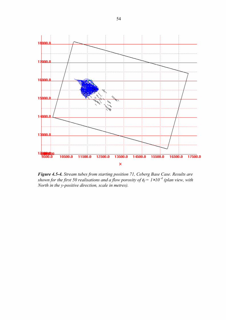
54
Figure 4.5-4. Stream tubes from starting position 71, Ceberg Base Case. Results areshown for the first 50 realisations and a flow porosity of εf = 1×10⁻⁴ (plan view, withNorth in the y-positive direction, scale in metres).
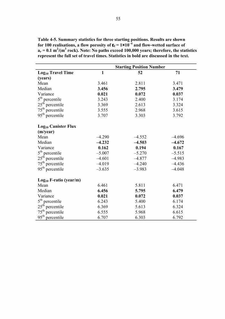
55
Table 4-5. Summary statistics for three starting positions. Results are shownfor 100 realisations, a flow porosity of εεf = 1××10–4 and flow-wetted surface ofar = 0.1 m2/(m3 rock). Note: No paths exceed 100,000 years; therefore, the statisticsrepresent the full set of travel times. Statistics in bold are discussed in the text.
Starting Position NumberLog10 Travel Time(years)
1 52 71
Mean 3.461 2.811 3.471
Median 3.456 2.795 3.479Variance 0.021 0.072 0.0375
th percentile 3.243 2.400 3.174
25th
percentile 3.369 2.613 3.324
75th
percentile 3.555 2.968 3.615
95th
percentile 3.707 3.303 3.792
Log10 Canister Flux(m/year)Mean –4.290 –4.552 –4.696
Median –4.232 –4.503 –4.672Variance 0.162 0.194 0.1675
th percentile –5.007 –5.270 –5.515
25th
percentile –4.601 –4.877 –4.983
75th
percentile –4.019 –4.240 –4.436
95th
percentile –3.635 –3.983 –4.048
Log10 F-ratio (year/m)Mean 6.461 5.811 6.471
Median 6.456 5.795 6.479Variance 0.021 0.072 0.0375
th percentile 6.243 5.400 6.174
25th
percentile 6.369 5.613 6.324
75th
percentile 6.555 5.968 6.615
95th
percentile 6.707 6.303 6.792

56
6
5
4
3
2
1
0
log(
Tra
vel T
ime)
[Yrs
]
100806040200Realisation Number
Ceberg, base case Position 1 Position 52 Position 71
Figure 4.5-5. Log10 travel time versus realisation number for three starting positionsin the Ceberg Base Case. Results are shown for100 realisations and a flow porosityof εf = 1×10⁻⁴.
-8
-6
-4
-2
0
log(
Can
iste
r F
lux)
[m3 /m
2 , Yrs
]
100806040200Realisation Number
Ceberg, base case Position 1 Position 52 Position 71
Figure 4.5-6. Log10 canister flux versus realisation number for three starting positionsin the Ceberg Base Case. Results are shown for100 realisations.

57
0.7
0.6
0.5
0.4
0.3
0.2
0.1
0.0
Fra
ctio
n
54321log(Travel Time) [Yrs]
Ceberg, base case Position 1 Position 52 Position 71
Figure 4.5-7. Smoothed frequency histogram of log10 travel time for three startingpositions in the Ceberg Base Case. Results are shown for 100 realisations and a flowporosity of εf = 1×10⁻⁴.
0.5
0.4
0.3
0.2
0.1
0.0
Fra
ctio
n
-8 -6 -4 -2 0log(Canister Flux) [m
3/m
2, Yrs]
Ceberg, base case Position 1 Position 52 Position 71
Figure 4.5-8. Smoothed frequency histogram of log10 canister flux for three startingpositions in the Ceberg Base Case. Results are shown for100 realisations.

59
5 Variant Cases
Table 5-1 summarises the Base Case (the reference case for comparison) and the four
variant cases evaluated for this study. Each of these variant simulations corresponds to
a possible interpretation of the site hydrogeology. These are summarised as follows:
• Base Case: Based on expert opinion, this model represents the expected site
conditions. This is the reference case for comparison to all other simulation results.
• Variant 1: Contrast between the conductor and rock domain (CD and RD) hydraulic
conductivities increased by a factor of 100.
• Variant 2: Alternative conductive features.
• Variant 3: Increased variance of log10 hydraulic conductivity.
• Variant 4: Simulation with a deterministic hydraulic conductivity field.
The Base Case is thoroughly discussed in Section 4. The motivation behind each variant
case is provided in the introductory section for each case. The results of each variant are
briefly compared to the Base Case in terms of the median and interquartile ranges of
the performance measures. A simple nonparametric hypotheses test determines the
statistical significance of the similarity of the performance measure distributions
(see Appendix A.2).

60
Table 5-1. Summary of Base and Variant Cases analysed in Ceberg site-scale modelling study.
BoundaryConditions
Hydraulic conductivity fieldCase
Obtainedfrom
Geostatisticalmodel
Hydraulic units EDZ/Backfill
Remarks
Base Case TR 97-21, caseGRST
Exponential,isotropic model,Variance 1.12Practical range 68m
CD: SCD1RD: SRD6(Walker et al.,1997b)
No/10–10 m/s
Variant #1
Increased Conductivity
Contrast
TR 97-21
case GRSFH
K in all CD
increased 100×Case GRSFH: All deterministic CD
increased by factor 100.
(Note: TR 97-23 proposed only 4 zones,
this study applies the increase to all zones
Variant #2
Alternative Conductive
Features
New regional
simulation case
GRSFZ; see
Appendix B
K in all CD
increased 100×Additional zones suggested by Saksa and
Nummela (1998).
Variant #3
Increased Conductivity
Variance
Variance of log10
hydraulic
conductivity = 2.0
Corresponding to covariance model based
on pooled data (SCD+SRD), i.e., larger
variance
Variant #4
Deterministic
Variance of log10
hydraulic
conductivity = 0
60
61
5.1 Increased Conductivity Contrast
The Base Case model for the site has assumed that the hydraulic conductivity of the
fracture zones is relatively similar to that of the rock mass. Although the values are
derived from the available on-site hydraulic tests, this low contrast in hydraulic
conductivity is unusual in comparison to the other SR 97 sites, Aberg and Beberg.
Some shallow percussion holes and 25 m packer tests suggest that the zones can be
quite conductive, even though the median hydraulic conductivity is quite low (Ahlbom
et al., 1983; Walker et al., 1997b). It is therefore reasonable to evaluate the possibility
that the hydraulic conductivity of the deterministic fracture zones is much higher than
that of the rock mass (Ahlbom et al., 1983; Walker et al., 1997b; Hermanson et al.,
1997).
As suggested in Walker et al. (1997b), the hydraulic conductivity of the rock mass
remains unchanged, but the hydraulic conductivity of the fracture zones given in Table
3-1 is increased by a factor of 100. This variant is similar to that of SCD4 as suggested
in Walker et al. (1997b), except that all the fracture zones have increased conductivity.
Figure 5.1-1 presents a plot of one realisation of the hydraulic conductivities for this
variant. The change in fracture conductivity might be expected to change the boundary
fluxes and heads, requiring a different set of boundary conditions from the regional
model. The regional model of Boghammar et al. (1997) included a corresponding
simulation, GRSFH, which this variant uses for site-scale boundary conditions. The
variant is otherwise unchanged from the Base Case, and uses 50 realisations.
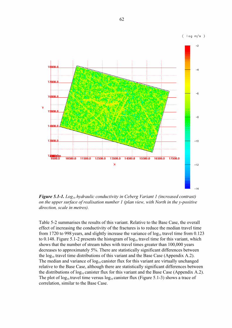
62
Figure 5.1-1. Log10 hydraulic conductivity in Ceberg Variant 1 (increased contrast)on the upper surface of realisation number 1 (plan view, with North in the y-positivedirection, scale in metres).
Table 5-2 summarises the results of this variant. Relative to the Base Case, the overall
effect of increasing the conductivity of the fractures is to reduce the median travel time
from 1720 to 998 years, and slightly increase the variance of log10 travel time from 0.123
to 0.148. Figure 5.1-2 presents the histogram of log10 travel time for this variant, which
shows that the number of stream tubes with travel times greater than 100,000 years
decreases to approximately 5%. There are statistically significant differences between
the log10 travel time distributions of this variant and the Base Case (Appendix A.2).
The median and variance of log10 canister flux for this variant are virtually unchanged
relative to the Base Case, although there are statistically significant differences between
the distributions of log10 canister flux for this variant and the Base Case (Appendix A.2).
The plot of log10 travel time versus log10 canister flux (Figure 5.1-3) shows a trace of
correlation, similar to the Base Case.

63
Table 5-2. Summary statistics for Ceberg Variant 1 (increased contrast).Results are shown for 50 realisations of 119 starting positions, a flow porosityof εεf = 1××10–4 and flow-wetted surface ar = 0.1 m2/(m3 rock). Statistics in boldare discussed in the text. Approximately 5% of the stream tubes fail to reachthe upper surface.
All values Travel Times > 100,000 yearsdeleted
Log10
tw
Log10
qc
Log10 F-ratio
Log10 tw Log10 qc Log10 F-ratio
Mean 3.061 –4.411 6.061 2.974 –4.407 5.974
Median 3.021 –4.423 6.021 2.999 –4.419 5.999Variance 0.311 0.212 0.311 0.148 0.212 0.1485
th percentile 2.306 –5.141 5.306 2.291 –5.135 5.291
25th
percentile 2.747 –4.712 5.747 2.732 –4.709 5.732
75th
percentile 3.291 –4.120 6.291 3.248 –4.114 6.248
95th
percentile 3.765 –3.663 6.765 3.560 –3.655 6.560
Histogram of log(Travel Time) : 50 realizations
log(Travel Time) [Yrs]
Fra
ctio
n
0.00
0.04
0.08
0.12
0.16
0.20
0.24
0.28
-2.0 -1.5 -1.0 -0.5 0.0 0.5 1.0 1.5 2.0 2.5 3.0 3.5 4.0 4.5 5.0 5.5 6.0
Figure 5.1-2. Relative frequency histogram of log10 travel time for Ceberg Variant 1(increased contrast). Results are shown for 50 realisations of 119 starting positions anda flow porosity of εf = 1×10⁻⁴.

64
Table 5-3 presents a comparison of the net volumetric flow of water across the
boundaries of the regional and site-scale models. The boundary flows for the site-scale
model have increased by a factor of 2 from the Base Case, reflecting the increased flow
in the deterministic fracture zones.
Table 5-3. Boundary flow consistency for Ceberg Variant 1 (increased contrast),regional model versus site-scale model.
The regional model mass balance residual is greater than 100% of the total outflow
from the site-scale domain. This error is attributed to the approximate mass balance
calculation technique and is not directly related to the boundary heads calculated by the
regional model.
To further investigate the boundary flows, this study constructs a mass balance for both
the regional and site-scale models, omitting the upper 200 m of the domain (i.e., the
upper surface of the mass balance control volume is lowered to –100 masl for both
models). Table 5-4 summarises the results, which show that the regional and site-scale
flows are within a factor of approximately 2. These results suggest that most of the
discrepancy between the regional and site-scale models occurs in the near surface
regions. This is attributed to mismatches in zone geometries and the use of calibrated
conductivities in the near surface of the Boghammar et al. (1997) regional model.
The regional mass balance residual is reduced to less than 40%, attributed to the
approximate method for calculating flows within finite elements of the regional model.
The regional mass balance residual of this variant is greater than the residual of the Base
Case because the accuracy of the approximation method decreases with increasing
hydraulic conductivity contrast (Section 4.2 and Appendix B.2).
Net Flow Through Site Model Surfaces (m3/s ×× 10–3)ModelSurface
Regional(GRSFH)
Variant 1 (5 realisations)
Base Case(5 realisations)
West 28.3 (in) 0.683 (in) 0.289 (in)
East 16.8 (out) 0.227 (out) 0.150 (in)
South 110.0 (out) 1.90 (out) 0.920 (out)
North 3.84 (out) 0.101 (out) 0.0995 (out)
Bottom 0.0639 (out) 0.152 (in) 0.0221 (in)
Top 273.0 (in) 1.39 (in) 0.557 (in)
Total Inflow 301.3 2.23 1.02
Total Outflow 130.7 2.23 1.02
Mass balance
(In – Out)
170.6 –0.003 –0.001
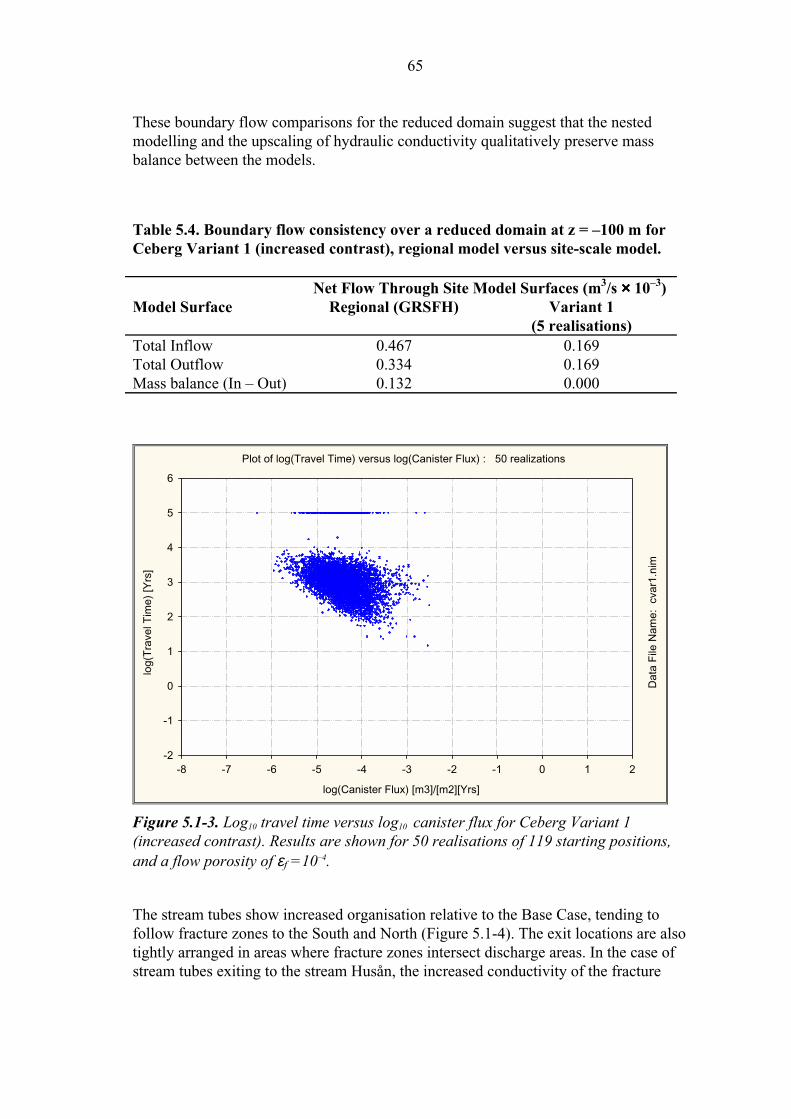
65
These boundary flow comparisons for the reduced domain suggest that the nested
modelling and the upscaling of hydraulic conductivity qualitatively preserve mass
balance between the models.
Table 5.4. Boundary flow consistency over a reduced domain at z = –100 m forCeberg Variant 1 (increased contrast), regional model versus site-scale model.
Net Flow Through Site Model Surfaces (m3/s ×× 10–3)Model Surface Regional (GRSFH) Variant 1
(5 realisations)Total Inflow 0.467 0.169
Total Outflow 0.334 0.169
Mass balance (In – Out) 0.132 0.000
Plot of log(Travel Time) versus log(Canister Flux) : 50 realizations
log(Canister Flux) [m3]/[m2][Yrs]
log(
Tra
vel T
ime)
[Yrs
]
Dat
a F
ile N
ame:
cva
r1.n
im
-2
-1
0
1
2
3
4
5
6
-8 -7 -6 -5 -4 -3 -2 -1 0 1 2
Figure 5.1-3. Log10 travel time versus log10 canister flux for Ceberg Variant 1(increased contrast). Results are shown for 50 realisations of 119 starting positions,and a flow porosity of εf =10–4.
The stream tubes show increased organisation relative to the Base Case, tending to
follow fracture zones to the South and North (Figure 5.1-4). The exit locations are also
tightly arranged in areas where fracture zones intersect discharge areas. In the case of
stream tubes exiting to the stream Husån, the increased conductivity of the fracture

66
zones results in the exit locations being shifted 1 km west to the western side of the mire
Stormyran (Figures 5.1-5).
The travel times, stream tubes and exit locations of this variant suggest that many of the
travel paths are diverted and accelerated as a result of increasing the conductivity of
the fracture zones. In addition to reducing the median travel times, this also tends to
increase the variance of travel time, since not all stream tubes follow fracture zones.
Increasing the fracture zone hydraulic conductivity appears to have little effect on the
canister flux, since the fracture zones do not intersect the starting positions representing
the hypothetical canisters.

67
Figure 5.1-4. Stream tubes in realisation number 1 of Ceberg Variant 1 (increasedcontrast). The y-positive axis of a) is rotated 15 cw from North. Results are shown for119 starting positions and a flow porosity of εf = 1×10⁻⁴.
N
N
a) Plan view
b) Elevation view, from South
c) Elevation view, from East
Approx. Scale
0 1000 m

68
18x103
16
14
12
10
(RA
K -
7 0
30 0
00),
Nor
th -
>
18x103 16141210
(RAK - 1 650 000), East ->
Husån
Flisbäcken
Västersjön
Skedmarkssjön
Gideån
Åktjärnen
Ceberg, variant 1
Model boundaries
----- Deposition tunnels
Exit locations
Figure 5.1-5. Exit locations for Ceberg Variant 1 (increased contrast). Results areshown for 50 realisations of 119 starting positions (plan view, scale in metres).

69
5.2 Alternative Conductive Features
In the site characterisation report, Ahlbom et al. (1983) suggests that the intrusive
dolerite and pegmatite dykes may be conductive features, with hydraulic conductivities
similar to the deterministic fracture zones. This has been questioned in later reports,
since such a characterisation cannot be unambiguously supported from the packer test
data (Hermanson et al., 1997). Similarly, Ahlbom et al. (1983) and Askling (1997) have
mapped an extensive topographic lineament running north-northwest to south-southeast
at the eastern margins of the site, which may be a fracture zone. However, the existence
of a fracture zone at this location cannot be unambiguously supported from the geo-
physical data (Hermanson et al., 1997). As part of SR 97, Saksa and Nummela (1998)
re-evaluated the site-scale structural model and suggested that both the intrusive dykes
and the topographic lineament might reasonably be interpreted as conductive fracture
zones.
This variant case evaluates the possibility that all of the fracture zones, the intrusive
dykes and the topographic lineaments are highly conductive fracture zones. Similar to
the variant discussed in Section 5.1, all of these features are assumed to have a hydraulic
conductivity 100 times those given in Table 3-1. Positions of the dykes and the regional
lineament are taken from Saksa and Nummela (1998) and are presented in Figure 3.5-2.
This variant is similar to that of SCD3, as suggested in Walker et al. (1997b), except
that this variant case includes all the intrusive dykes as well as the regional lineament.
Because this additional regional lineament might change the boundary fluxes and heads,
this variant requires a slightly different regional model than that used by the Base Case.
The regional model of Boghammar et al. (1997) was rerun for this study to provide site-
scale boundary conditions (Case GRSFZ, described in Appendix B). The variant is
otherwise unchanged from the Variant 1, and uses 50 realisations.
Figure 5.2-1 presents the HYDRASTAR representation of the fracture zones used in this
variant, and Figures 5.2-2 and 5.2-3 show the additional zones relative to the repository
tunnels. These figures illustrate that the additional fracture zones are very close to the
hypothetical repository, with one of the east-west trending dolerite dykes (Dolerite 1)
running directly through the repository block. The utility program TRAZON checked
the additional zones versus the starting positions (Appendix E). In contrast to the Base
Case and all other variants, several starting positions fall into the conductive features of
this variant. Seven starting positions, numbered 4, 9, 26, 39, 41, 54 and 56, fall into
Dolorite 1 (Figure 3.4-2). Figure 5.2-4 presents one realisation of the resulting hydraulic
conductivity field.

70
Figure 5.2-1. HYDRASTAR representation of fracture zones in Ceberg Variant 2(alternative conductors). (Plan view, with North in the y-positive direction, scale inmetres).
Figure 5.2-2. HYDRASTAR representation of the four additional fracture zones inCeberg Variant 2 (alternative conductors). (Plan view, with North in the y-positivedirection, scale in metres).

71
Figure 5.2-3. The repository tunnels relative to the four additional fracture zones inCeberg Variant 2 (alternative conductors). (Detail of Figure 5.2-2).
Figure 5.2-4. Log10 hydraulic conductivity field in Ceberg Variant 2 (alternativeconductors) on the upper surface of realisation 1. (Plan view, with North in they-positive direction, scale in metres).

72
Table 5-5 summarises the effects of including the additional structures, where approxi-
mately 3.6% of the stream tubes fail to reach the upper surface. In comparison to the
Base Case, the median travel time is reduced from 1720 to 800 years, and the variance
of log10 travel time is increased from 0.123 to 0.307. These results are similar to those
of Variant 1, where many of the stream tubes are intercepted by conductive features,
decreasing the median of travel time while increasing the variance of log10 travel time.
In this variant, the effect is stronger because one of the conductive features runs directly
through the repository (Dolerite 1), creating a set of stream tubes that has a much faster
travel time than the remainder of the set. The resulting log10 travel time distribution
for this variant is markedly skewed and there are statistically significant differences
between the log10 travel time distributions of this variant versus those of Variant 1
and the Base Case (Appendix A.2; Figure 5.2-5). Unlike Variant 1, the median
canister flux is increased from 3.27 ×10
–5 to 4.3×10
–5 m/year, also a consequence of
Dolerite 1 passing directly through the repository zone, intercepting seven starting
Histogram of log(Travel Time) : 50 realizations
log(Travel Time) [Yrs]
Fra
ctio
n
0.00
0.04
0.08
0.12
0.16
0.20
0.24
-2.0 -1.5 -1.0 -0.5 0.0 0.5 1.0 1.5 2.0 2.5 3.0 3.5 4.0 4.5 5.0 5.5 6.0
Figure 5.2-5. Relative frequency histogram for log10 travel time in Ceberg Variant 2(alternative conductors). Results are shown for 50 realisations of 119 starting positionsand a flow porosity of εf = 1×10⁻⁴.
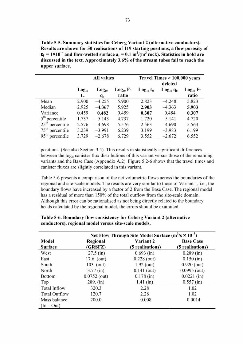
73
Table 5-5. Summary statistics for Ceberg Variant 2 (alternative conductors).Results are shown for 50 realisations of 119 starting positions, a flow porosity ofεεf = 1××10–4 and flow-wetted surface ar = 0.1 m2/(m3 rock). Statistics in bold arediscussed in the text. Approximately 3.6% of the stream tubes fail to reach theupper surface.
All values Travel Times > 100,000 yearsdeleted
Log10
tw
Log10
qc
Log10 F-ratio
Log10 tw Log10 qc Log10 F-ratio
Mean 2.900 –4.255 5.900 2.823 –4.248 5.823
Median 2.925 –4.367 5.925 2.903 –4.363 5.903Variance 0.459 0.482 0.459 0.307 0.484 0.3075
th percentile 1.737 –5.143 4.737 1.720 –5.141 4.720
25th
percentile 2.576 –4.698 5.576 2.563 –4.690 5.563
75th
percentile 3.239 –3.991 6.239 3.199 –3.983 6.199
95th
percentile 3.729 –2.678 6.729 3.552 –2.672 6.552
positions. (See also Section 3.4). This results in statistically significant differences
between the log10 canister flux distributions of this variant versus those of the remaining
variants and the Base Case (Appendix A.2). Figure 5.2-6 shows that the travel times and
canister fluxes are slightly correlated in this variant.
Table 5-6 presents a comparison of the net volumetric flows across the boundaries of the
regional and site-scale models. The results are very similar to those of Variant 1, i.e., the
boundary flows have increased by a factor of 2 from the Base Case. The regional model
has a residual of more than 150% of the total outflow from the site-scale domain.
Although this error can be rationalised as not being directly related to the boundary
heads calculated by the regional model, the errors should be examined.
Table 5-6. Boundary flow consistency for Ceberg Variant 2 (alternativeconductors), regional model versus site-scale models.
Net Flow Through Site Model Surface (m3/s ×× 10–3)ModelSurface
Regional(GRSFZ)
Variant 2 (5 realisations)
Base Case(5 realisations)
West 27.5 (in) 0.693 (in) 0.289 (in)
East 17.6 (out) 0.228 (out) 0.150 (in)
South 103. (out) 1.92 (out) 0.920 (out)
North 3.77 (in) 0.141 (out) 0.0995 (out)
Bottom 0.0752 (out) 0.178 (in) 0.0221 (in)
Top 289. (in) 1.41 (in) 0.557 (in)
Total Inflow 320.3 2.28 1.02
Total Outflow 120.7 2.28 1.02
Mass balance
(In – Out)
200.0 –0.008 –0.0014
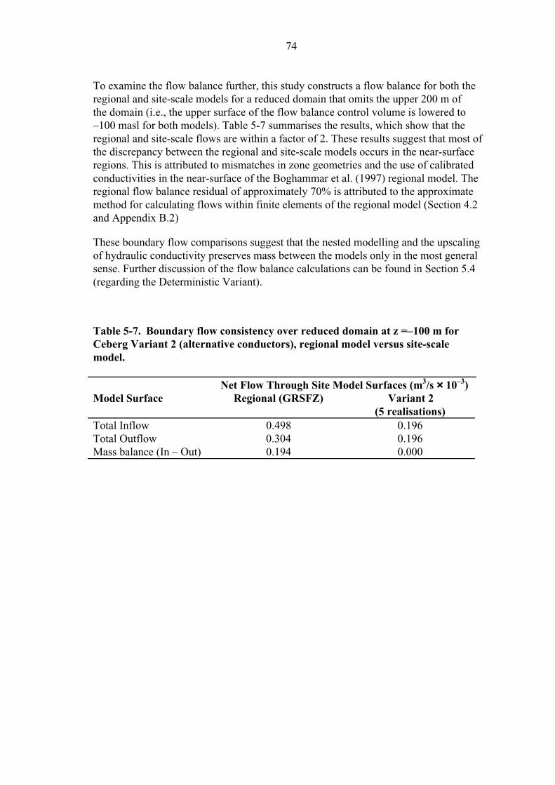
74
To examine the flow balance further, this study constructs a flow balance for both the
regional and site-scale models for a reduced domain that omits the upper 200 m of
the domain (i.e., the upper surface of the flow balance control volume is lowered to
–100 masl for both models). Table 5-7 summarises the results, which show that the
regional and site-scale flows are within a factor of 2. These results suggest that most of
the discrepancy between the regional and site-scale models occurs in the near-surface
regions. This is attributed to mismatches in zone geometries and the use of calibrated
conductivities in the near-surface of the Boghammar et al. (1997) regional model. The
regional flow balance residual of approximately 70% is attributed to the approximate
method for calculating flows within finite elements of the regional model (Section 4.2
and Appendix B.2)
These boundary flow comparisons suggest that the nested modelling and the upscaling
of hydraulic conductivity preserves mass between the models only in the most general
sense. Further discussion of the flow balance calculations can be found in Section 5.4
(regarding the Deterministic Variant).
Table 5-7. Boundary flow consistency over reduced domain at z =–100 m forCeberg Variant 2 (alternative conductors), regional model versus site-scalemodel.
Net Flow Through Site Model Surfaces (m3/s ×× 10–3)Model Surface Regional (GRSFZ) Variant 2
(5 realisations)Total Inflow 0.498 0.196
Total Outflow 0.304 0.196
Mass balance (In – Out) 0.194 0.000

75
Plot of log(Travel Time) versus log(Canister Flux) : 50 realizations
log(Canister Flux) [m3]/[m2][Yrs]
log(
Tra
vel T
ime)
[Yrs
]
Dat
a F
ile N
ame:
cva
r2.n
im
-2
-1
0
1
2
3
4
5
6
-8 -7 -6 -5 -4 -3 -2 -1 0 1 2
Figure 5.2-6. Log10 travel time versus log10 canister flux for Ceberg Variant 2(alternative conductors). Results are shown for 50 realisations of 119 startingpositions and a flow porosity of εf = 1×10⁻⁴.
Similar to Variant 1, the stream tubes show increased organisation relative to the Base
Case, tending to follow fracture zones to the South and North (Figure 5.2-7). The exit
locations are also tightly arranged in areas where fracture zones intersect discharge
areas. In the case of stream tubes exiting to the stream Husån, the increased conductivity
of the fracture zones results in the exit locations being shifted 1 km west to the western
side of the mire Stormyran (Figures 5.2-8).
The travel times, stream tubes and exit locations of this variant suggest that many of the
travel paths are diverted and accelerated as a result of increasing the conductivity of
the fracture zones. In addition to reducing the median travel times, this also tends to
increase the variance of travel time, since not all stream tubes follow fracture zones.
Comparing the results to Variant 1, the canister flux effects of this variant are attributed
to the dolerite dykes intersecting the starting positions representing the hypothetical
canisters. The results of Variants 1 and 2 taken together suggest that reasonable
assumptions regarding the occurrence, extent and properties of the conductive
features may have a strong impact on the performance assessment.
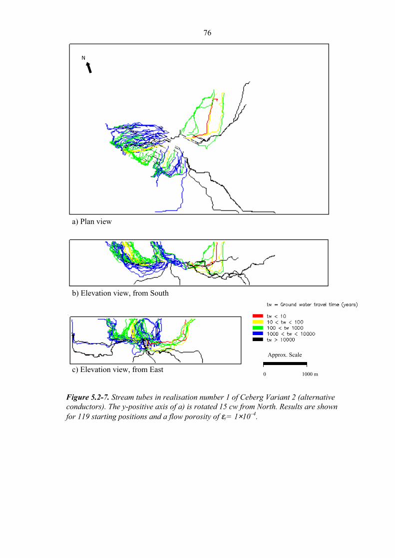
76
Figure 5.2-7. Stream tubes in realisation number 1 of Ceberg Variant 2 (alternativeconductors). The y-positive axis of a) is rotated 15 cw from North. Results are shownfor 119 starting positions and a flow porosity of εf = 1×10⁻⁴.
N
a) Plan view
b) Elevation view, from South
Approx. Scale
0 1000 mc) Elevation view, from East

77
18x103
16
14
12
10
(RA
K -
7 0
30 0
00),
Nor
th -
>
18x103 16141210
(RAK - 1 650 000), East ->
Husån
Flisbäcken
Västersjön
Skedmarkssjön
Gideån
Åktjärnen
Ceberg, variant 2
Model boundaries
----- Deposition tunnels
Exit locations
Figure 5.2-8. Exit locations for Ceberg Variant 2 (alternative conductors). Results areshown for 50 realisations of 119 starting positions (plan view, scale in metres).

78
5.3 Increased Conductivity Variance
The Base Case geostatistical model was inferred from the packer test data in the rock
mass domain (SRD), resulting in a log10 hydraulic conductivity variance of 1.12
(Appendix C). It is possible that using the SRD data separately may have under-
estimated the variance; for example, the pooled data set of SRD and SCD data has a
variance of 2.5 (Walker et al, 1997b). The simulations in Variant 3 were performed with
a log10 hydraulic conductivity variance of 2.0 to evaluate the impacts of this uncertainty.
This variant is otherwise unchanged from the Base Case, including the fact that the
same mean log10 hydraulic conductivities are used for this variant as for the Base Case.
Figure 5.3-1 presents one realisation of the resulting hydraulic conductivity field.
Because the increased variance may reduce the stability of the Monte Carlo simulations,
it is important to check the stability of the statistics of interest versus the number of
realisations. Figure 5.3-2 presents a plot of the median of log10 travel time. The figure
shows little change in the estimates beyond 30 realisations.

79
Figure 5.3-1. Log10 hydraulic conductivity in Ceberg Variant 3 (increased variance)on the upper surface of realisation number 1 (plan view, with North in the y-positivedirection, scale in metres).

80
Median of log(Travel Time) as related to number of realizations
(Based on Travel Times less than 100 000 years)
Number of Realizations
log(
Tra
vel T
ime)
[Yrs
]
2.96
3.00
3.04
3.08
3.12
3.16
3.20
3.24
0 10 20 30 40 50
Figure 5.3-2. Monte Carlo stability of median travel time for Ceberg Variant 3(increased variance). Results shown for a flow porosity of εf = 1×10⁻⁴.
Table 5-8 summarises the results of this simulation. Relative to the Base Case, the
variance of log10 travel time increases from 0.123 to 0.156 and variance of log10 canister
flux increases from 0.182 to 0.295. The median log10 travel time decreases from 1720
to 1130 years, and the median log10 canister flux increases from 3.27×10⁻⁵
m/year to
4.59×10⁻⁵
m/year. Approximately 11% of the stream tubes fail to reach the upper
surface.
Table 5-8. Summary statistics for Ceberg Variant 3 (increased variance).Results are shown for 50 realisations of 119 starting positions, a flow porosityof εεf = 1××10–4 and flow-wetted surface ar = 0.1 m2/(m3 rock). Statistics in bold arediscussed in the text. Approximately 11% of the stream tubes fail to reach theupper surface.
All values Travel Times > 100,000 yearsdeleted
Log10
tw
Log10
qc
Log10 F-ratio
Log10 tw Log10 qc Log10 F-ratio
Mean 3.258 –4.351 6.258 3.038 –4.350 6.038
Median 3.117 –4.338 6.117 3.052 –4.337 6.052Variance 0.522 0.295 0.522 0.156 0.296 0.1565
th percentile 2.403 –5.268 5.403 2.382 –5.264 5.382
25th
percentile 2.808 –4.709 5.808 2.764 –4.710 5.764
75th
percentile 3.439 –3.962 6.439 3.314 –3.955 6.314
95th
percentile 5.000 –3.485 8.000 3.671 –3.481 6.671

81
These reflect the statistically significant differences between distributions of this variant
and the Base Case for both log10 travel time and log10 canister flux (Appendix A.2;
Figure 5.3-3). Log10 travel time and log10 canister flux appear to be slightly correlated,
but little different from the Base Case (Figure 5.3-4). The stream tubes and exit loca-
tions (Figures 5.3-5 and 5.3-6) appear to be organised along fracture zones, similar to
Variant 2.
Although the increased variances can be explained as the result of the increased variance
of log10 hydraulic conductivity, the decreased travel times, increased canister flux, and
increased boundary flows indicate an overall increase in hydraulic conductivity. A
hueristic explanation for this apparent increase is provided by the Gutjahr et al. (1978)
solution for the effective conductivity of an isotropic domain:
Where Ke is the effective hydraulic conductivity of the domain, Kg is the geometric
mean of point values of hydraulic conductivity (K) within the domain, and 2
ln Kσ is the
variance of lnK. (Dagan, 1993, and Abramovich and Indelman, 1995, discuss higher
order approximations). This relationship suggests that increasing only the variance of
hydraulic conductivity increases the overall conductivity of the domain, and thus we
should expect increased fluxes and decreased travel times.
Table 5-9 indicates that the boundary flows through the domain appear to be increased
by a factor of 3, confirming that the increased variance has resulted in an increased
effective conductivity. The boundary flow comparison also indicates that the site-scale
model underpredicts the regional model flows by a factor of seven. There is also a 10%
regional mass balance residual. Although this error can be rationalised as not being
directly related to the boundary heads calculated by the regional model, the high error
should be examined.
To further investigate the boundary flows, this study constructs a mass balance for both
the regional and site-scale models for domain that omits the upper 200 m of the domain
(i.e., the upper surface of the mass balance control volume is lowered to –100 masl for
both models). Table 5-10 summarises the results, which show that the regional flows
are closely approximated by the site-scale flows. These results suggest that most of the
discrepancy between the regional and site-scale models occurs in the near surface
regions. This is attributed to mismatches in zone geometries and the use of calibrated
conductivities in the near surface of the Boghammar et al. (1997) regional model. The
regional mass balance residual is reduced to approximately 6% and is attributed to the
approximate method for calculating mass balance within finite elements of the regional
model (Section 4.1 and Appendix B.2).
+=
61
2
ln Kge KK
σ
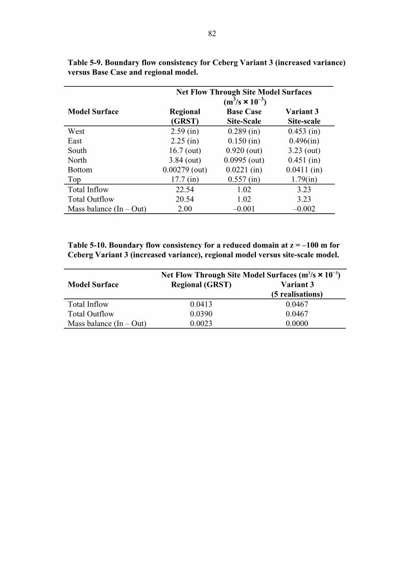
82
Table 5-9. Boundary flow consistency for Ceberg Variant 3 (increased variance)versus Base Case and regional model.
Net Flow Through Site Model Surfaces (m3/s ×× 10–3)
Model Surface Regional(GRST)
Base CaseSite-Scale
Variant 3 Site-scale
West 2.59 (in) 0.289 (in) 0.453 (in)
East 2.25 (in) 0.150 (in) 0.496(in)
South 16.7 (out) 0.920 (out) 3.23 (out)
North 3.84 (out) 0.0995 (out) 0.451 (in)
Bottom 0.00279 (out) 0.0221 (in) 0.0411 (in)
Top 17.7 (in) 0.557 (in) 1.79(in)
Total Inflow 22.54 1.02 3.23
Total Outflow 20.54 1.02 3.23
Mass balance (In – Out) 2.00 –0.001 –0.002
Table 5-10. Boundary flow consistency for a reduced domain at z = –100 m forCeberg Variant 3 (increased variance), regional model versus site-scale model.
Net Flow Through Site Model Surfaces (m3/s ×× 10–3)Model Surface Regional (GRST) Variant 3
(5 realisations)Total Inflow 0.0413 0.0467
Total Outflow 0.0390 0.0467
Mass balance (In – Out) 0.0023 0.0000
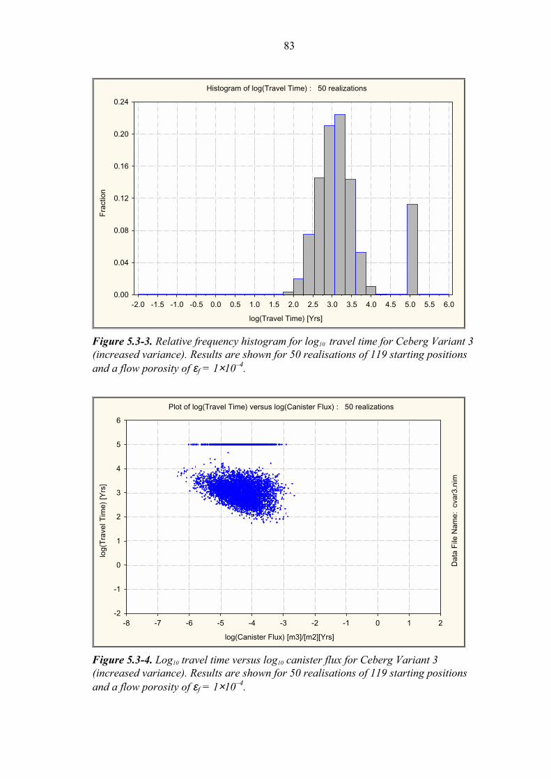
83
Histogram of log(Travel Time) : 50 realizations
log(Travel Time) [Yrs]
Fra
ctio
n
0.00
0.04
0.08
0.12
0.16
0.20
0.24
-2.0 -1.5 -1.0 -0.5 0.0 0.5 1.0 1.5 2.0 2.5 3.0 3.5 4.0 4.5 5.0 5.5 6.0
Figure 5.3-3. Relative frequency histogram for log10 travel time for Ceberg Variant 3(increased variance). Results are shown for 50 realisations of 119 starting positionsand a flow porosity of εf = 1×10⁻⁴.
Plot of log(Travel Time) versus log(Canister Flux) : 50 realizations
log(Canister Flux) [m3]/[m2][Yrs]
log(
Tra
vel T
ime)
[Yrs
]
Dat
a F
ile N
ame:
cva
r3.n
im
-2
-1
0
1
2
3
4
5
6
-8 -7 -6 -5 -4 -3 -2 -1 0 1 2
Figure 5.3-4. Log10 travel time versus log10 canister flux for Ceberg Variant 3(increased variance). Results are shown for 50 realisations of 119 starting positionsand a flow porosity of εf = 1×10⁻⁴.

84
Figure 5.3-5. Stream tubes in realisation number 1 of Ceberg Variant 3 (increasedvariance). The y-positive axis of a) is rotated 15 cw from North. Results are shown for119 starting positions and a flow porosity of εf = 1×10⁻⁴.
N
a) Plan view
b) Elevation view, from South
c) Elevation view, from East
Approx. Scale
0 1000 m

85
18x103
16
14
12
10
(RA
K -
7 0
30 0
00),
Nor
th -
>
18x103 16141210
(RAK - 1 650 000), East ->
Husån
Flisbäcken
Västersjön
Skedmarkssjön
Gideån
Åktjärnen
Ceberg, variant 3
Model boundaries
----- Deposition tunnels
Exit locations
Figure 5.3-6. Exit locations for Ceberg Variant 3 (increased variance). Results areshown for 50 realisations of 119 starting positions (plan view, scale in metres).

86
5.4 Deterministic Simulation
This variant is a simplified representation of the site using a deterministic hydraulic
conductivity field (i.e., the field has no random component and thus requires only one
‘realisation’). The objectives of this simulation are to further evaluate the empirical
upscaling and nested modelling, and to examine the effects of the large-scale hetero-
geneity (e.g., the fracture zones and rock blocks). As was discussed in Sections 4.2, 5.1
and Appendix C.1, choosing the appropriate hydraulic conductivities is complicated by
the apparent scale dependence of hydraulic conductivity. This study uses the empirical
upscaling rule (Appendix C.1) to determine the effective conductivity, Ke, for the SRD
and each SCD. If the nested modelling and upscaling are consistent, the boundary flows,
travel times and canister fluxes should be approximately the same for both the Base
Case and this Deterministic Variant.
Table 5-11 presents the effective conductivities of each unit. Note that for this variant,
there is no block-scale variability (zero variance, thus no spatial variability of hydraulic
conductivity except for the contrast between the rock domain and conductor domain).
Figure 3.5-5 shows the deterministic field.
Table 5-11. Ceberg deterministic model for hydraulic conductivity, with 25 mmeasurements and 35 m grid scale shown for comparison. Upscaled as inAppendix C.1.
Elevation (masl) 25 m MeanLog10 K (m/s)
35 m MeanLog10 K (m/s)
Deterministic (100 m)Log10 K (m/s)
SCD+110 to 0 –7.0 –6.9 –6.4
0 to –100 –8.5 –8.4 –7.9
–100 to –300 –9.5 –9.4 –8.9
Below –300 –9.7 –9.6 –9.1
SRD+110 to 0 –7.6 –7.4 –7.2
0 to –100 –9.0 –8.9 –8.7
–100 to –300 –10.0 –9.9 –9.6
Below –300 –10.3 –10.1 –9.9
Table 5-12 summarises the results of this deterministic simulation in terms of the travel
time, canister flux and F-ratio averaged over all the starting positions. Approximately
9.2% of the stream tubes fail to reach the upper surface. Note that the median travel time
is 1790 years and median canister flux is 3.40×10⁻⁵
m/year, both very similar to those of
the Base Case. In comparison to the Base Case, the variance of log10 canister flux is
much lower at 0.007 because the hydraulic conductivity field has no spatial variability.
In contrast to the canister flux, the variance of log10travel time for this variant is 0.096,
relatively unchanged from the Base Case. This suggests that the variability of travel
times is due to the differences in starting position relative to the exit location, and not
due to heterogeneity of the host rocks. This low variability is also seen in the smooth,
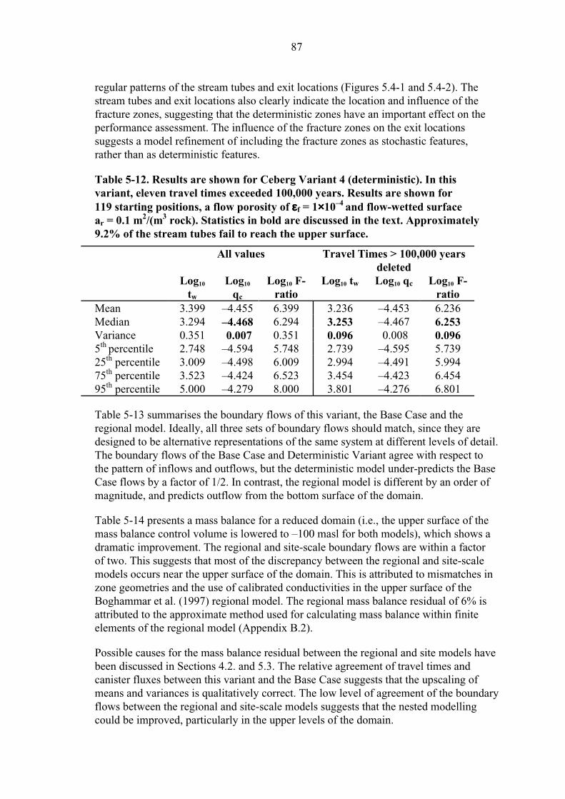
87
regular patterns of the stream tubes and exit locations (Figures 5.4-1 and 5.4-2). The
stream tubes and exit locations also clearly indicate the location and influence of the
fracture zones, suggesting that the deterministic zones have an important effect on the
performance assessment. The influence of the fracture zones on the exit locations
suggests a model refinement of including the fracture zones as stochastic features,
rather than as deterministic features.
Table 5-12. Results are shown for Ceberg Variant 4 (deterministic). In thisvariant, eleven travel times exceeded 100,000 years. Results are shown for119 starting positions, a flow porosity of εεf = 1××10–4 and flow-wetted surfacear = 0.1 m2/(m3 rock). Statistics in bold are discussed in the text. Approximately9.2% of the stream tubes fail to reach the upper surface.
All values Travel Times > 100,000 yearsdeleted
Log10
tw
Log10
qc
Log10 F-ratio
Log10 tw Log10 qc Log10 F-ratio
Mean 3.399 –4.455 6.399 3.236 –4.453 6.236
Median 3.294 –4.468 6.294 3.253 –4.467 6.253Variance 0.351 0.007 0.351 0.096 0.008 0.0965
th percentile 2.748 –4.594 5.748 2.739 –4.595 5.739
25th
percentile 3.009 –4.498 6.009 2.994 –4.491 5.994
75th
percentile 3.523 –4.424 6.523 3.454 –4.423 6.454
95th
percentile 5.000 –4.279 8.000 3.801 –4.276 6.801
Table 5-13 summarises the boundary flows of this variant, the Base Case and the
regional model. Ideally, all three sets of boundary flows should match, since they are
designed to be alternative representations of the same system at different levels of detail.
The boundary flows of the Base Case and Deterministic Variant agree with respect to
the pattern of inflows and outflows, but the deterministic model under-predicts the Base
Case flows by a factor of 1/2. In contrast, the regional model is different by an order of
magnitude, and predicts outflow from the bottom surface of the domain.
Table 5-14 presents a mass balance for a reduced domain (i.e., the upper surface of the
mass balance control volume is lowered to –100 masl for both models), which shows a
dramatic improvement. The regional and site-scale boundary flows are within a factor
of two. This suggests that most of the discrepancy between the regional and site-scale
models occurs near the upper surface of the domain. This is attributed to mismatches in
zone geometries and the use of calibrated conductivities in the upper surface of the
Boghammar et al. (1997) regional model. The regional mass balance residual of 6% is
attributed to the approximate method used for calculating mass balance within finite
elements of the regional model (Appendix B.2).
Possible causes for the mass balance residual between the regional and site models have
been discussed in Sections 4.2. and 5.3. The relative agreement of travel times and
canister fluxes between this variant and the Base Case suggests that the upscaling of
means and variances is qualitatively correct. The low level of agreement of the boundary
flows between the regional and site-scale models suggests that the nested modelling
could be improved, particularly in the upper levels of the domain.

88
Table 5-13. Boundary flow consistency of Ceberg Variant 4 (deterministic) andBase Case, regional model versus site-scale models.
Net Flow Through Site Model Surfaces (m3/s ×× 10–3)
Model Surface Regional (GRST) Site-scale:Base Case
Site-scale:Deterministic
West 2.59 (in) 0.289 (in) 0.100 (in)
East 2.25 (in) 0.150 (in) 0.0649 (in)
South 16.7 (out) 0.920 (out) 0.411 (out)
North 3.84 (out) 0.0995 (out) 0.0927 (out)
Bottom 0.00279 (out) 0.0221 (in) 0.0196 (in)
Top 17.7 (in) 0.557 (in) 0.320 (in)
Total Inflow 22.54 1.02 0.505
Total Outflow 20.54 1.02 0.504
Mass balance (In – Out) 2.00 –0.0014 0.0008
Table 5-14. Boundary flow consistency for a reduced domain at z = –100 m forCeberg Variant 4 (deterministic), regional model versus site-scale models.
Net Flow Through Site Model Surfaces (m3/s ×× 10–3)Model Surface Regional
(GRST)Base Case Deterministic Case
(5 realisations) (5 realisations)Total Inflow 0.0413 0.0262 0.0230
Total Outflow 0.0390 0.0262 0.0230
Mass balance (In – Out) 0.0023 0.000 0.0000

89
Figure 5.4-1. Stream tubes in realisation number 1 of Ceberg Variant 4 (deterministic).The y-positive axis of a) is rotated 15 cw from North. Results are shown for 119 startingpositions and a flow porosity of εf = 1×10⁻⁴.
N
a) Plan view
b) Elevation view, from South
c) Elevation view, from East
Approx. Scale
0 1000 m

90
18x103
16
14
12
10
(RA
K -
7 0
30 0
00),
Nor
th -
>
18x103 16141210
(RAK - 1 650 000), East ->
Husån
Flisbäcken
Västersjön
Skedmarkssjön
Gideån
Åktjärnen
Ceberg, variant 4
Model boundaries
----- Deposition tunnels
Exit locations
Figure 5.4-2. Exit locations for Ceberg Variant 4 (deterministic). Results are shown for119 starting positions (plan view, scale in metres).
91
6 Discussion and Summary
The SKB SR 97 study is a comprehensive performance assessment illustrating the
results for three hypothetical repositories in Sweden. This study addresses the
hydrogeologic modelling of Ceberg, one of three sites, via the application of
HYDRASTAR, a stochastic continuum groundwater flow-modelling program. The
application is relatively straightforward, with the majority of the model parameters
explicitly specified in Walker et al. (1997b). This section of the report summarises the
simulations and discusses the results of the study in terms of statistics for travel time,
F-ratio and canister flux. It also summarises the findings of the study with regard to
model parameter uncertainty, as evaluated by the variant cases.
The study results are broadly summarised by the statistics of the common logarithm
transforms of the travel times, canister fluxes and F-ratios to facilitate summary (Table
6.1). The results for the Base Case and the variants are directly compared in plots of
their floating histograms in Figures 6.2-1 and 6.2-2 (note that Variant 4 is excluded
because its low performance measure variances; see Appendix A.1 for the computation
of the floating histograms).
6.1 Input Data
Input data for the model are unmodified from that given in Walker et al. (1997b) except
for the empirical rescaling of hydraulic conductivities as suggested by Walker et al.
(1997b). The SKB geostatistical analysis code INFERENS is used to infer a regularised
variogram model, based on the 25 m interpreted hydraulic conductivities taken from
SICADA.
The boundary conditions for this model are constant head boundaries, taken from a
deterministic regional scale model of Boghammar et al. (1997). The overall groundwater
flow pattern of the regional model is typical of topographically-driven systems, with
recharge in the uplands discharging to valleys. The regional heads are transferred to
the site-scale model via constant head boundaries, generally preserving the regional
flow pattern in the site-scale model. The mass balance between the nested models is
presented via a comparison of net volumetric flow of water over the site-scale model
boundaries. Adjustment of the scaling of hydraulic conductivity to fine-tune the
boundary flows is not pursued.

92
6.2 Base Case
The Base Case uses 100 realisations of 119 stream tube starting positions to evaluate the
canister fluxes, travel times, and F-ratios for the proposed repository. As discussed in
Section 4.0, the median travel times and median canister fluxes of the Base Case appear
to be stable with respect to the number of simulations. The boundary flows of the
regional model and the site-scale model appeared to be consistent with respect to
orientation, but the site-scale model underpredicts the boundary flows of the regional
model by a factor of 20. Detailed analysis of these flows indicates that the inconsistency
occurs near the upper model surface and that the nested models and the upscaling of
hydraulic conductivity generally preserve mass balance over the majority of the domain.
A comparison of the Base and Deterministic (Variant 4) Cases indicates that the
upscaling is approximately self-consistent with respect to median travel time, median
canister flux and boundary flows.
Floating Histogram of Log10(Travel Time)
for Different Variants for Ceberg
0.0
0.1
0.2
0.3
0.4
0.5
0.6
0.7
0.8
0.9
1.0
-2 -1 0 1 2 3 4 5 6
Log10(Travle Time) [years]
Fre
qu
ency
Base CaseVariant 1
Variant 2Variant 3
Figure 6.2-1. Summary of Ceberg modelling results: floating histogram of log10 traveltime normalised to the number of travel times less than 100,000 years. Results areshown for 119 starting positions and a flow porosity of εf = 1×10⁻⁴.

93
Floating Histogram of Log10(Canister Flux)
for Different Variants for Ceberg
0.0
0.1
0.2
0.3
0.4
0.5
0.6
0.7
0.8
0.9
1.0
-7 -6 -5 -4 -3 -2 -1 0 1
Log10(Canister Flux) [m3/m2,year]
Fre
qu
ency
Base CaseVariant 1
Variant 2
Variant 3
Figure 6.2-2. Summary of Ceberg modelling results: floating histogram of log10 canisterflux normalised to the total number of stream tubes.
The results for 100 realisations of 119 starting positions with a flow porosity of
εf = 1×10⁻⁴
and a flow-wetted surface area of ar = 0.1 m2/(m
3 rock) suggest the
following results for the Base Case:
• The median travel time is 1720 years with an interquartile range from 953 to 2965
years.
• The median canister flux is 3.27×10⁻⁵
m/year with an interquartile range from
1.66×10⁻⁵
to 6.25×10⁻⁵
m/year.
• The median F-ratio is 1.72×10⁶ year/m with an interquartile range from 9.53×10
5
to 2.97×10⁶ year/m.
The current version of HYDRASTAR is limited to homogeneous flow porosity over the
entire domain. Consequently, the F-ratio is a simple multiple of the travel time, and the
log10 canister flux has a slight, inverse correlation with travel time. The stream tubes and
exit locations of the realisations are compatible with the overall pattern of flow at the
site. Approximately 10% of the stream tubes fail to reach the upper surface of the
model domain, with most of these stream tubes exiting the southern model boundary.
Approximately 1% of the total number of stream tubes exit the bottom surface of the
model, directly beneath the site.

94
Three realisations are examined to illustrate the variability within each realisation, and
are compared to illustrate the variability between realisations of the Monte Carlo set.
The variability within a realisation due to spatial variability is rather high, but the exit
locations are relatively stable between realisations. The variability between realisations
for median travel time and median canister flux is relatively low.
Three individual starting positions are examined over all 100 realisations to illustrate
variability due to the differences in location. These positions demonstrate that some
areas have shorter travel times (e.g., the southwestern side of the repository). This is
attributed to the starting position relative to the discharge area and flow pattern, rather
than to spatial variability of the host rock hydraulic conductivity.
6.3 Variant Cases
6.3.1 Increased Conductivity Contrast
This variant addresses the possibility that the deterministic fracture zones can be quite
conductive, even though the median hydraulic conductivity of the fracture zones
inferred from the hydraulic tests is quite low. As suggested in Walker et al. (1997b),
the hydraulic conductivity of the rock mass remains unchanged, but the hydraulic
conductivity of the fracture zones is increased by a factor of 100. The regional
modelling study of Boghammar et al. (1997) provided a set of boundary conditions
appropriate for increased fracture zone hydraulic conductivities, different from the
regional model used for the Base Case. Most of the boundary flow inconsistencies
between the regional and site-scale models occur in the upper model surfaces.
The overall effect of increasing the conductivity of the fractures is to reduce the median
travel time to 998 years, and slightly increase the variance of log10 travel time to 0.148.
These results reflect travel paths being diverted and accelerated as a result of increasing
the conductivity of the fracture zones. Stream tubes and exit locations are organised
around fracture zones, and exit locations near the stream Husån are shifted 1 km to the
west. Canister flux is essentially unchanged from the Base Case, since the fracture zones
do not intersect the starting positions representing the hypothetical canisters. There are
statistically significant differences between the results of this variant and those of the
Base Case. The inverse correlation of travel times and canister fluxes is stronger in this
variant than in the Base Case.
6.3.2 Alternative Conductive Features
This variant case evaluates the possibility that the intrusive dykes and one additional
regional lineament are conductive features. Similar to the variant discussed in Section
4.2, these fractures are assumed to have a hydraulic conductivity 100 times that of the
Base Case. The additional regional lineament requires a new set of boundary conditions,
95
which are provided by a new simulation based on the regional model of Boghammar
et al. (1997) (Appendix B). Most of the boundary flow inconsistencies between the
regional and site-scale models occur in the upper model surface.
In comparison to the Base Case, the median travel time is reduced to 800 years, and
the variance of log10 travel time is increased to 0.307. The travel time distribution is
markedly skewed and the median canister flux is slightly increased to 4.3×10⁻⁵
,
reflecting the fracture zones intersecting the repository zone. The inverse correlation of
travel times and canister fluxes is stronger in this variant than in the Base Case. These
results are similar to those of Variant 1, where many of the stream tubes are intercepted
by conductive features, decreasing the median travel time while increasing the variance
of log10 travel time. The effect is stronger in this variant because one of the conductive
features runs directly through the repository. Unlike Variant 1, the median canister flux
is increased as a consequence of one of the alternative features passing through the
repository zone, intercepting seven starting positions. There are statistically significant
differences between the results of this variant and those of the Base Case. Similar to
Variant 1, the stream tubes are organised along fracture zones, and exit locations near
the stream Husån are shifted 1 km to the west.
6.3.3 Increased Conductivity Variance
The simulations in Variant 3 are performed to evaluate the uncertainties associated
with the inference of the variance of hydraulic conductivity. For this variant case, the
variance of log10 hydraulic conductivity is increased from 1.12 to 2.0. The mean
conductivities for the rock mass domain and the fracture zone domain are identical to
the Base Case. The increased variance does not appear to have reduced the stability of
the Monte Carlo simulations. Excluding the upper model surface, the boundary flows
for the regional and site-scale models are in good agreement.
Relative to the Base Case, the variances of log10 travel time and log10 canister flux
increase, reflecting the increased variance. The median travel time decreases to 1130
years, and the median canister flux increases to 4.59×10⁻⁵
m/year. The increased
boundary and canister fluxes, and the decreased travel time conceptually agree with the
predictions of stochastic continuum theory regarding the effective conductivity of the
domain. There are statistically significant differences between the results of this variant
and those of the Base Case. Flow patterns for this variant appear little different from
those of the Base Case.
6.3.4 Deterministic Simulation
This variant is a simplified simulation of the site using a deterministic representation of
the hydraulic conductivity field (i.e., the field has no random component and thus needs
only one ‘realisation’). This study uses the empirical upscaling rule to estimate the
effective conductivity of the deterministic field. Note that for this variant, there is no
block-scale variability (zero variance).

96
Relative to the Base Case, the variance of log10 travel time is reduced only slightly to
0.096, suggesting that the travel time variability in the Base Case is due to the difference
in starting positions relative to the flow pattern. The variance of log10 canister flux is
much lower at 0.007, as is expected for a deterministic hydraulic conductivity field.
Similar to the Base Case, the median travel time is 1790 years and the median canister
flux is 3.40×10⁻⁵
m/year, suggesting that the upscaling of hydraulic conductivity is
approximately self-consistent.
6.3.5 Comparison
Table 6-1 presents a summary of the medians and variances of the performance
measures for the Base Case (in bold) and for Variants 1 through 4. Variant 2,
Alternative Conductive Features, yields the shortest median travel time. Variant 4,
Deterministic Simulation, yields the longest median travel time but is very similar to
the Base Case. Variant 3, Increased Variance, yields the maximum median canister
flux, and the Base Case yields the minimum median canister flux.
Note that the Base Case variability nearly encompasses the full range of variability
exhibited by the variant cases. For example, the Base Case travel time has an inter-
quartile range from 953 to 2965 years, while the range of median travel times for the
variants is from 800 years (Variant 2) to 1790 years (Variant 4). Thus the variability of
the Base Case due to parameter variability is approximately the same as the variability
of the cases studied to address uncertainty. Within the limitations of the variant cases
studied, this suggests that the Base Case has adequately characterised the Ceberg
hypothetical performance. Similarly, although there are statistically significant
differences between the distributions of the performance measures among all the
cases, the differences between the cases are believed to be minor in the context of
performance assessment.

97
Table 6-1. Summary of Ceberg site-scale modelling study. Results are shown for 119 starting positions, a flow porosity of εεf = 1××10–4
and flow-wetted surface ar = 0.1 m2/(m3 rock). Statistics in bold are discussed in the text.
PerformanceMeasure
Statistic Base Case Variant 1(FZ Contrast)
Variant 2(Alt. CD)
Variant 3(Increased Var.)
Variant 4(Deterministic)
Log10 Travel time Median 3.236 2.999 2.903 3.052 3.253
(years, for travel
times less than
100,000 years)
Variance 0.123 0.148 0.307 0.156 0.096
Log10 Canister
Flux
Median –4.485 –4.423 –4.367 –4.338 –4.468
(m/year, for all
starting positions)
Variance 0.182 0.212 0.482 0.295 0.007
Log10 F-ratio Median 6.236 5.999 5.903 6.052 6.253
(year/m, for travel
times less than
100,000 years)
Variance 0.123 0.148 0.307 0.156 0.096
97

98
6.4 Possible Model Refinements
This modelling study evaluates the groundwater flow system at the Ceberg site, using a
model that incorporates the processes believed to dominate the site groundwater system.
This includes Base Case simulations of the expected site conditions, and several Variant
Cases that evaluate uncertainties. Although the study is considered adequate for
performance assessment, there are additional variant cases that may be of interest.
It is possible to examine several additional variants and model refinements within
the current features of HYDRASTAR. For example, extending the model domain
downward and southward might capture and quantify the stream tubes that fail to exit
the upper surface of the model. The variability of hydraulic conductivity with depth is
uncertain, and could be evaluated with a variant case for an alternative representation
of the depth trend of hydraulic conductivity. It should be noted, however, that the
uncertainties evaluated by these possible variants are believed to have only a minor
effect on the performance assessment.
Other model refinements are possible but are outside of the current features of
HYDRASTAR. These include experimentation with alternative upscaling methods
and the use of alternative methods of representing the hydraulic conductivities (e.g.,
nonparametric geostatistical simulation, or discrete feature networks upscaled to
numerical block conductivities, stochastic fracture zones, etc.). Ultimately, because
of the dominating effect of the boundary conditions, such refinements may not have a
profound impact on the performance measures. The relative importance of the boundary
conditions, however, suggests a variant case to investigate the effects of using constant
flux (Neuman) or third-type boundaries instead of the present constant head (Dirichlet)
boundaries. Lastly, Variants 1 and 2 suggest refining the regional model flow balance to
reduce the apparent residual of the regional model and make the flow balance a more
powerful modelling tool.
6.5 Summary of Findings
The findings of this study can be summarised as follows. With regard to the usage of
data and consistency with the regional model, the parameters are consistent with field
observations, and are unmodified except for the rescaling of hydraulic conductivity
inherent to stochastic continuum modelling. The majority of the boundary flow
inconsistencies between the regional and site-scale models appear to occur in the
near-surface regions of the models.
With regard to the variability seen within realisations, there is great spatial variability
seen in the travel times and canister fluxes within single realisations. This variability
appears to be the result of the position of the hypothetical canisters relative to the
discharge areas, rather than to the spatial variability of the host rocks.
99
The results for 100 realisations of 119 starting positions, a flow porosity of εf = 1×10⁻⁴
and a flow-wetted surface area of ar = 0.1 m2/(m
3 rock) suggest the following results for
the Base Case:
• The median travel time is 1720 years with an interquartile range from 953 to 2965
years.
• The median canister flux is 3.27×10⁻⁵
m/year with an interquartile range from
1.66×10⁻⁵
to 6.25×10⁻⁵
m/year.
• The median F-ratio is 1.72×10⁶ year/m with an interquartile range from 9.53×10
5
to 2.97×10⁶ year/m.
• The common logarithm of canister flux appears to be inversely correlated to the
common logarithm of travel time.
• The stream tubes and exit locations are compatible with the flow pattern at the site.
The uncertainties of this study are addressed by a series of variant cases that evaluate
the sensitivity of the results to changes in assumptions regarding the structural model
and the hydraulic conductivities. The results are most sensitive to the occurrence
of additional highly conductive features such as fracture zones or intrusive dykes,
particularly if such features directly intersect with the waste canisters. However, it is
reasonable to assume that such features would be avoided in the placement of waste
canisters. Although the approach to upscaling appears to be approximately self-
consistent, the nested modelling approach and the regional model mass balance
could be re-examined.

101
Acknowledgements
The authors of this report would like to acknowledge the support and guidance
of Anders Ström and Jan-Olof Selroos of the Swedish Nuclear Fuel and Waste
Management Company (SKB). This study has benefited enormously from the review
comments of Johan Andersson and Sven Follin of Golder Grundteknik, and Ingvar
Rhén, VBB VIAK. Raymond Munier of Scandia Consult and Lee Hartley of AEA
Technology have contributed data, ideas and useful comments throughout this study.
Lydia Biggs (DE&S) contributed a number of illustrations and formatting suggestions
to this report. The final text has benefited enormously from the careful editing of
Marcie Summerlin (DE&S).
At the end of a long study, it is tempting to list all of modelling team members as
coauthors of the final report, but this would be a practical impossibility for this report.
The efforts of the following contributors are appreciated and are hereby acknowledged:
• Maria Lindgren and Hans Widén (Kemakta) implemented the structural model and
assisted in setting up the HYDRASTAR model for this study.
• Niko Marsic (Kemakta) postprocessed the model output to provide the statistical
summaries of results, and Lars Lovius (Hellström and Lovius Data) provided general
support for the HYDRASTAR simulations and postprocessing of results.
• Björn Bergman (DE&S) performed the scoping calculations for travel time, and
along with Cecilia Andersson (DE&S) assisted in preparing the preliminary sections
of the report.
• Gregory Ruskauff (DE&S) assisted in the geostatistical analysis and helped review
and summarise the study.
• Lee Hartley (AEA Technology) supported the NAMMU regional model simulations
and assisted in the preparation of Appendix B.
This study was funded by The Swedish Nuclear Fuel and Waste Management Company
(SKB).

103
References
Abramovich B and Indelman P, 1995. Effective permeability of log-normal isotropic
random media. J. Phys. A: Math. Gen., 28, p 693–700.
Ahlbom K, Albino B, Carlsson L, Nilsson G, Olsson O, Stenberg L and Timje H,1983. Evaluation of the geological, geophysical and hydrogeological conditions at
Gideå. Swedish Nuclear Fuel and Waste Management Co., SKBF/KBS Technical
Report TR 83-53, Stockholm, Sweden.
Ahlbom K, Andersson J-E, Nordqvist R, Ljunggren C, Tirén S and Voss C, 1991.Gideå study site. Scope of activities and main results. Swedish Nuclear Fuel and Waste
Management Co., SKB Technical Report TR 91-51, Stockholm, Sweden.
Andersson J, 1999. SR 97 – Data and data uncertainties: Compilation of data and
evaluation of data uncertainties for radionuclide transport calculations, Swedish
Nuclear Fuel and Waste Management Co., SKB Technical Report TR-99-09,
Stockholm, Sweden.
Askling P, 1997. Gideå lineament map. An interpretation based on elevation data
models. Swedish Nuclear Fuel and Waste Management Co., SKB Progress Report
PR U-97-06, Stockholm, Sweden.
Björck S and Svensson N-O, 1992. Climatic changes and uplift patterns – past, present
and future. Swedish Nuclear Fuel and Waste Management Co., SKB Technical Report
TR 92-38, Stockholm, Sweden.
Boghammar A and Marsic N, 1997. Using Statistica when evaluating results from
HYDRASTAR 1.5+. Swedish Nuclear Fuel and Waste Management Co., SKB Progress
Report PR U-97-18, Stockholm, Sweden.
Boghammar A, Grundfelt B and Hartley L, 1997. Investigation of the large
scale regional hydrogeological situation at Ceberg. Swedish Nuclear Fuel and Waste
Management Co., SKB Technical Report TR 97-21, Stockholm, Sweden.
Carlsson L, Winberg A and Grundfelt B, 1983. Model calculations of the ground-
water flow at Finnsjön, Fjällveden, Gideå and Kamlunge. SKBS KBS Technical Report
TR 83-45, Stockholm, Sweden.
Cliffe K A, Jackson C P and Morris S T, 1995. Assessment Model Validity
Document; NAMMU: A program for calculating groundwater flow and transport
through porous media. Swedish Nuclear Fuel and Waste Management Co., SKB
Working Report AR 95-11, Stockholm, Sweden.

104
Dagan G, 1986. Statistical theory of groundwater flow and transport: pore to laboratory,laboratory to formation, and formation to regional scale. Water Resources Research,22(9), p 1205–1345.
Dagan G, 1993. High-order correction of effective permeability of heterogeneousisotropic formations of lognormal conductivity distributions. Transport in PorousMedia, 12, p 279–290.
de Marsily G, Lavedan C, Boucher M and Fasanino G, 1984. Interpretationof Interference Tests in a Well Field Using Geostatistical Techniques to Fit thePermeability Distribution in a Reservoir Model, in Geostatistics for Natural ResourcesCharacterisation. Second NATO Advanced Study Institute, GEOSTAT 1983, TahoeCity, California. Edited by G. Verly, M. David, A.G. Journel, and A. Marachal,p 831–849, D. Reidel, Hingham, MA, USA.
Ericsson L O, and Ronge B, 1986. Correlations between tectonic lineaments andpermeability values of crystalline bedrock in the Gideå area. Swedish Nuclear Fueland Waste Management Co., SKB Technical Report TR 86-19, Stockholm, Sweden.
Geier J, 1993. Verification of the geostatistical inference code INFERENS, Version1.1, and demonstration using data from Finnsjön. Swedish Nuclear Fuel and WasteManagement Co., SKB Technical Report TR 93-09, Stockholm, Sweden.
Gutjahr A L, Gelhar L W, Baker A A and MacMillan J R, 1978. Stochasticanalysis of spatial variability in subsurface flows. 2. Evaluation and application.Water Resources Research, 14(5), p 953–959.
Gylling B, Lindgren M and Wid én H, 1999a. Preparatory hydrogeologicalcalculations for site scale models of Aberg, Beberg, and Ceberg. Swedish NuclearFuel and Waste Management Co., SKB Report R-99-06, Stockholm, Sweden.
Gylling B, Walker D and Hartley L, 1999b. Site-scale groundwater flow modelling ofBeberg. Swedish Nuclear Fuel and Waste Management Co., SKB Technical Report inpreparation, Stockholm, Sweden.
Hammersley J M and Handscomb D C, 1975. Monte Carlo Methods. Methuen,London.
Hermanson J, Hansen L M and Follin S, 1997. Update of the geological modelsof the Gideå study site. Swedish Nuclear Fuel and Waste Management Co., SKB ReportR-97-05, Stockholm, Sweden.
Hodgkinson D P and Barker J, 1985. Specification of a Test Problem forHYDROCOIN Level 1 Case1: Transient Flow from a Borehole in a FracturedPermeable Medium. Report AERE R-11574, UK Atomic Energy Authority, HarwellLaboratories, UK.

105
Hultman S, 1997. Visualisation of HYDRASTAR Simulation Data in the AVS 5System. Swedish Nuclear Fuel and Waste Management Co., SKB Progress ReportPR U-97-01, Stockholm, Sweden.
Journel A G and Huijbregts Ch J, 1978. Mining Geostatistics. Academic Press.
Laaksoharju J, Skårman C and Gurban I, 1998. SR 97: Summary of Hydro-geochemical conditions at Aberg, Beberg and Ceberg. Swedish Nuclear Fuel andWaste Management Co., SKB Technical Report TR 98-03, Stockholm, Sweden.
Larsen R J and Marx M L, 1986. An Introduction to Mathematical Statistics and ItsApplications. Prentice-Hall, London.
Leake S A, Lawson P W, Lilly M R and Claar D V, 1998. Assignment of boundaryconditions in embedded groundwater flow models. Ground Water 36(4), p 621–625.
Lovius L, 1998. Calculation of flux through boundaries in HYDRASTAR. SwedishNuclear Fuel and Waste Management Co., SKB Progress Report PR U-98-08,Stockholm, Sweden.
Lovius L and Eriksson L, 1993. Verification of HYDRASTAR version 1.4. SwedishNuclear Fuel and Waste Management Co., SKB Working Report AR 93-46, Stockholm,Sweden.
Lovius L and Eriksson L, 1994. Development of a transient version of HYDRASTAR.Swedish Nuclear Fuel and Waste Management Co., SKB Working Report AR 94-12,Stockholm, Sweden.
Lundqvist T, Gee D, Karis L, Kumpulainen R and Kresten P, 1990. Beskrivning tillberggrundskartan över Västernorrlands Län (in Swedish with an English summary).SGU ser. BA 31. Geological Survey of Sweden, Uppsala.
Marsic N, 1999. Using STATISTICA and MATLAB when evaluating results fromHYDRASTAR 1.5+. Swedish Nuclear Fuel and Waste Management Co., SKB ProgressReport TS-99-04, Stockholm, Sweden.
Morris S T and Cliffe K A, 1994. Verification of HYDRASTAR: Analysis ofhydraulic conductivity fields and dispersion. Swedish Nuclear Fuel and WasteManagement Co., SKB Technical Report TR 94-21, Stockholm, Sweden.
Munier R, Sandstedt H and Niland L, 1997. Förslag till principiella utformningar avförvar enligt KBS-3 för Aberg, Beberg and Ceberg. Swedish Nuclear Fuel and WasteManagement Co., SKB Report R 97-09, Stockholm, Sweden.
Neuman S, 1988. A proposed conceptual framework and methodology for investigatingflow and transport in Swedish crystalline rocks. Swedish Nuclear Fuel and WasteManagement Co., SKB Working Report AR 88-37, Stockholm, Sweden.

106
Neuman S and Jacobson E, 1984. Analysis of nonintrisic spatial variability by residualkriging with application to regional groundwater levels. Mathematical Geology, 16(5),p 499–521.
Norman S, 1991. Verification of HYDRASTAR – A code for stochastic continuumsimulation of groundwater flow. Swedish Nuclear Fuel and Waste Management Co.,SKB Technical Report TR 91-27, Stockholm, Sweden.
Norman S, 1992a. Statistical inference and comparison of stochastic models for thehydraulic conductivity at the Finnsjön-site. Swedish Nuclear Fuel and WasteManagement Co., SKB Technical Report TR 92-08, Stockholm, Sweden.
Norman S, 1992b. HYDRASTAR – A code for stochastic simulation of groundwaterflow. Swedish Nuclear Fuel and Waste Management Co., SKB Technical ReportTR 92-12, Stockholm, Sweden.
OECD, 1983. The International HYDROCOIN Project: Groundwater hydrologymodelling strategies for performance assessment of nuclear waste disposal. Level: Codeverification.
Renard Ph and de Marsily G, 1997. Calculating equivalent permeability: a review.Advances in Water Resources, 20 (5,6), p 253–278.
Rhén I, Gustafson G, Stanfors R and Wikberg P, 1997. Äspö Hard RockLaboratory – Geoscientific Evaluation 1997/5. Models based on site characterisation1986–1995. Swedish Nuclear Fuel and Waste Management Co., SKB Technical ReportTR 97-06, Stockholm, Sweden.
Rubin Y and Gómez-Hernández J J, 1990. A stochastic approach to the problemof upscaling of conductivity in disordered media: Theory and unconditional numericalsimulations. Water Resources Research, 26(4), p 691–701.
Saksa P and Nummela J, 1998. Geological-structural models used in SR 97:Uncertainty analysis. Swedish Nuclear Fuel and Waste Management Co., SKBTechnical Report TR 98-12, Stockholm, Sweden.
SKB, 1992. SKB 91: Final disposal of spent nuclear fuel. Importance of bedrock forsafety. Swedish Nuclear Fuel and Waste Management Co., SKB Technical ReportTR 92-20, Stockholm, Sweden.
SKB, 1996a. SR-95: Template for safety reports with descriptive example. SwedishNuclear Fuel and Waste Management Co., SKB Technical Report TR 96-05,Stockholm, Sweden.
SKB, 1996b. User’s Guide to HYDRASTAR 1.5. Swedish Nuclear Fuel and WasteManagement Co., SKB Progress Report PR-U-96-15, Stockholm, Sweden.

107
Timje H, 1983. Hydrogeological investigations at study site Gideå. Swedish NuclearFuel and Waste Management Co., SKBF/KBS Working Report AR 83-26 (in Swedish),Stockholm, Sweden.
Walker D and Bergman B, 1998. Verification of HYDRASTAR v.1.7: Transientsimulation and pilot point calibration. Swedish Nuclear Fuel and Waste ManagementCo., SKB Progress Report in preparation, Stockholm Sweden.
Walker D and Gylling B, 1998. Site-scale groundwater flow modelling of Aberg.Swedish Nuclear Fuel and Waste Management Co., SKB Technical Report TR 98-23,Stockholm, Sweden.
Walker D, Lovius L and Eriksson L, 1997a. Verification of HYDRASTAR 1.7:Nugget effect in geostatistical simulations. Swedish Nuclear Fuel and WasteManagement Co., SKB Progress Report, PR U-97-22, Stockholm, Sweden.
Walker D, Rhén I and Gurban I, 1997b. Summary of Hydrogeologic Conditionsat Aberg, Beberg and Ceberg. Swedish Nuclear Fuel and Waste Management Co., SKBTechnical Report 97-23, Stockholm, Sweden.
Ward D, Buss D, Mercer J and Hughes S, 1987. Evaluation of a groundwatercorrective action at the Chem-Dyne hazardous waste site using a telescopic meshrefinement modelling approach. Water Resources Research, 23(4), p 603–617.

109
Appendix A. Definition of Statistical Measures
A.1 Floating Histograms
This study generally uses binned histograms to display the frequency distributions of the
performance measures. The bin width of such histograms is determined by the default
algorithms of Statistica. Although the bin width is somewhat subjective, binned
histograms do provide a relatively unprocessed image of the data. However, binned
histograms are not well suited to graphical comparisons (e.g. overlaying multiple binned
histograms is confusing to the eye).
An alternative method of constructing a frequency distribution histogram is to use a
floating histogram. Floating histograms are single curved line representations of the
frequency of the data. Although floating histograms are smoothed representations of
the data, they are more legible when superimposed for the comparison of multiple
histograms. Depending on the format and type of data being processed, several software
packages (Appendix F) are used to calculate the floating histograms using a moving
window as a filter passing over the ordered sequence of the data. For each datum value
centred in the window, the smoothed frequency is calculated as the fraction of the data
falling within the window. The width of the window is somewhat arbitrarily set to ± ½
an order of magnitude around the datum value in the centre of the window, and the
frequency of each window is normalised by dividing by the total number of data.
Generally, MATLAB is used to calculate the moving window statistics, and the
histograms displayed in Excel. The exception to this is Figure 4.3-11, which is
calculated and plotted using Statistica. The floating histograms of Variant 4, the
Deterministic Case, are omitted, since the low performance measure variances result
in virtually the entire distribution falling within the smoothing window.
A.2 Statistical Significance of the Comparison ofDistributions
Section 5 makes a number of comparisons of variant cases versus the Base Case or
versus other variants, concluding that ‘there are statistically significant differences
between the distributions’. This statement of significance is quantitatively supported
by a statistical comparison of the distributions, testing the null hypothesis:
H0: the distributions are the same
The significance of this test, or p-value, is the probability of rejecting H0 when it is in
fact true (a so-called Type I error). Thus, a small p-value indicates that we can safely
reject the hypothesis that the distributions are the same (Larsen and Marx, 1986).
Because the distributions to be compared in this study are skewed, they are not suited

110
to test statistics that assume normally (Gaussian) distributed data. This study therefore
uses nonparametric (distribution-free) test statistics to compute the p-value of the above
test. The Kolmogorov-Smirnov test (K-S) is a nonparametric test used to compare
distributional shapes (i.e., skewness, variability, and location), as documented in the
Statistica manual. The p-value of a K-S test of H0 is computed for the various
combinations of the Base Case and variant cases (Table A-1).
Note: When computing the p-value for the comparisons of log10 travel time
distributions, times greater than the default maximum travel time of 100,000 years
are deleted from the distributions prior to the comparison. The resulting K-S p-value
therefore ignores the stream tubes failing to exit the upper surface of the model.
Table A-1 Test for Similarity of Travel Time Distributions (Kolmogorov-Smirnov2-sample).
Case Base Variant 1 Variant 2 Variant 3Base reject(p<0.001) reject(p<0.001) reject(p<0.001)
Variant 1 reject(p<0.001) reject(p<0.001) reject(p<0.001)
Variant 2 reject(p<0.001) reject(p<0.001) reject(p<0.001)
Variant 3 reject(p<0.001) reject(p<0.001) reject(p<0.001)
Canister FluxCase Base Variant 1 Variant 2 Variant 3Base reject(p<0.001) reject(p<0.001) reject(p<0.001)
Variant 1 reject(p<0.001) reject(p<0.001) reject(p<0.001)
Variant 2 reject(p<0.001) reject(p<0.001) reject(p<0.001)
Variant 3 reject(p<0.001) reject(p<0.001) reject(p<0.001)
111
Appendix B. Supplemental Regional Simulation
B.1 Variant 2 Regional Model
This appendix reproduces the following memo: Additional Variant of the Regional
Scale Hydrogeology at Ceberg, L.J. Hartley, AEA Technology, November 1998.
This memo describes the regional model used to create boundary conditions for Variant
Case 2. The memo is included without modification, except for deletion of figures and
several minor edits to correct references to other reports.
B.1.1 Introduction
This note documents an additional variant on the regional groundwater flow at Ceberg
performed on behalf of SKB as part of the SR 97 safety assessment project. All other
SR 97 regional-scale groundwater flow calculations for Ceberg are detailed in
Boghammar et al. (1997). The purpose of the variant is to assess the impact of several
extra site-scale fracture zones and a high contrast in hydraulic conductivity between
the fracture zones and the rock mass. The extra calculation is performed for the small
regional model (GRS) only. The resulting pressure distribution has been used to set
boundary conditions for an equivalent site-scale variant.
B.1.2 Alternative Conductive Features (GRSFX)
In the site characterisation report, Ahlbom et al. (1983) suggests that the intrusive
dolerite and pegmatite dykes may be conductive features, with hydraulic conductivities
similar to the deterministic fracture zones. This has been questioned in later reports,
since such a characterisation cannot be unambiguously supported from the packer test
data (Hermanson et al., 1997). Similarly, Ahlbom et al. (1983) and Askling (1997) have
mapped an extensive topographic lineament running north-northwest to south-southeast
at the eastern margins of the site, which may be a fracture zone. However, the existence
of a fracture zone at this location cannot be unambiguously supported from the
geophysical data (Hermanson et al., 1997). As part of SR 97, Saksa and Nummela
(1998) re-evaluated the site-scale structural model and suggested that both the intrusive
dykes and the topographic lineament might reasonably be interpreted as conductive
fracture zones.
This variant case evaluates the possibility that the fracture zones, the intrusive dykes
and the topographic lineaments are all highly conductive fracture zones. Similar to the
GRSFH variant, these fractures are assumed to have a hydraulic conductivity 100 times
that used in the Base Case.

112
Topographic head boundary conditions are used. Positions of the dykes and the regional
lineament are taken from Saksa (personal communication, 1998) and are presented in
Saksa and Nummela (1998). This variant is similar to that of SCD3, as suggested in
Walker et al. (1997b), except that all the intrusive dykes are included, as is the regional
lineament.
The pathlines are similar to the GRSFH variant, except a few paths now reach greater
depths (1500 m). This is likely to be caused by the extra zones creating a larger recharge
rate, which drives some flow paths deeper. The spatial distribution of discharge areas
varies little from the GRSFH and is consistent with the Base Case (GRST), but there
are none of the horizontally extensive paths that are seen in the GRST or GRSN Cases.
A comparison of initial Darcy velocity and travel time for the GRSFX variant and the
Base Case is constructed for a uniform array of 16 start points within the site region at
z = –350 m. For six of the start positions, the Darcy velocity is 20–100 times larger in
the GRSFX case than in the Base Case. The higher velocity is due to these paths starting
within one of the site-scale fracture zones. The travel time for these paths is corre-
spondingly shorter, some as low as 10–100 years. For the remaining start positions, the
travel time is still on average about 1000 years, suggesting that the initial part of these
paths is through the rock mass, causing an increase in the travel time.
B.2 Regional Model Mass Balance Calculations
Several sections of this report have discussed the mass balance of the regional model in
terms of the net volumetric flow of water across the boundaries of site-scale domain,
but Boghammar et al. (1997) did not document these quantities. The regional flows
discussed in this study were provided in a series of personal communications and
unpublished memos by Lee Hartley of AEA Technology. What follows is a summary of
those memos and discussions describing the post-processing of NAMMU simulations to
approximate the regional model flows across the site-scale HYDRASTAR domain for
the Base (GRST), Variant 1 (GRSFH) and Variant 2 (GRSFZ) Cases.
The mass balance computations use the small-scale regional NAMMU model for the
Gideå (GRS) to determine the net volumetric flows (m3/s) through the six planar faces
of a cube coincident with the boundaries of the site-scale model. The NAMMU code
uses the finite element method of solving the governing equations for groundwater flow,
a numerical method that inherently preserves mass balance over the element faces. In
addition, NAMMU uses a direct solver, so that the solution to the system of equations is
exact within the accuracy of the host platform. That is, regardless of the approximate
mass balance over arbitrary subdomains, the finite element method and NAMMU’s
direct solver insure that mass balance is preserved and that the resulting simulated heads
are correct (Cliffe et al, 1995).
However, the cube faces of the site-scale model do not necessarily coincide with
element faces of the regional model. For this study, the regional flows over the site-scale
domain were estimated by sampling the outward normal flux (specific discharge, m/s) at
a regular grid of points on each face of the cube. The spacing of sample points was set at

113
10 m in the horizontal directions and 3 m in the vertical. The finite elements of the
regional model are typically about 100 m on a side, so the sample points are close
enough to resolve the variation in permeability and hence velocity with depth. The
net volumetric flow out of each face was taken as the sum of pointwise fluxes at each
sample, multiplied by the cross-sectional area (m2) represented by each sampling point.
The sampling grid was refined until the calculated flows converged to a stable value,
and mass balance residuals were computed for all three regional cases. These residuals
reflect the sampling errors of this approximating method, and it is expected that a more
rigorous approach (i.e., Gaussian quadrature within each element) would reduce this
error dramatically. In addition, the mass balance is particularly poor for GRSFH and
GRSFZ because groundwater velocity is very heterogeneous in these cases, reducing
the accuracy of the approximation.
(Lee Hartley, personal communication, 1998).

115
Appendix C. Supplemental Calculations
C.1 Upscaling of Hydraulic Conductivity Model
C.1.1 Approach
The injection tests performed in the cored boreholes are the principal source of
hydraulic conductivity data. These tests were interpreted and the measurements reported
for various depths, rock types, etc. as described by Ahlbom et al. (1983). The interpreted
hydraulic conductivities for the 25 m packer tests were taken directly from the SKB
SICADA database and analysed with the SKB geostatistical inference code INFERENS.
The scale of these measurements (as inferred from the packer length) is much different
from the proposed model grid scale. As discussed in Walker et al. (1997b) and Renard
and de Marsily (1997), hydraulic conductivity is a scale-dependent parameter, which
requires that the measured hydraulic conductivities be upscaled to the finite difference
grid scale of the model. Thus, HYDRASTAR requires rescaling the geometric means
of interpreted hydraulic conductivities found in SICADA. This study uses the scaling
relationship provided in Rhén et al. (1997), which assumes that the geometric mean of
hydraulic conductivity at the measurement scale, Lm, may be adjusted for scale using the
regression equation:
)(782.010101010 mugmgu LLogLLogKLogKLog −+=
where:
Kg = geometric mean of hydraulic conductivity (m/s)
L = length scale (m), assumed equal to the packer interval.
The subscripts m and u refer to the measurement and upscaled values, respectively.
Rhén et al. (1997) developed this empirical scaling relationship using the 3 m, 30 m,
100 m packer tests and full-length tests in the same cored boreholes.
C.1.2 Base Case (35 m scale) Model
The inference of spatial correlation models for Ceberg site-scale hydraulic conductivity
begins by dividing the domain into SRD, SCD and elevation zones. The elevation zones
and SCD are treated as step changes in the mean of log10 conductivities, and a single
variogram model is inferred for the entire domain (i.e., the same variogram for SRD and
SCD). The Äspö scaling relationships of Rhén et al. (1997) are used to determine the

116
geometric mean of hydraulic conductivity in each SRD and depth zone (Appendix C.1).
The effect of upscaling on the variogram is determined by applying the Moye’s formula-
based regularisation algorithm and fitting a variogram–trend model via iterative
generalised least squares estimation (IGLSE; see Neuman and Jacobsen, 1984) to the
regularised data. The SKB program INFERENS, which includes the Moye’s formula-
based regularisation, automates the IGLSE fitting algorithm. Program restrictions of
HYDRASTAR and INFERENS limit the geostatistical model to one variogram model
for both domains. Because the majority of the 25 m packer tests fall in the SRD and
these data yield a clearer variogram, the geostatistical model will be developed from the
interpreted hydraulic conductivities in the SRD.
The Moye’s formula-based regularisation has one additional restriction, in that it only
works for regularisation scales that are multiples of the packer interval; e.g., 25 m data
can be regularised to 50 m, 75 m, etc. for the Gideå data. That is, the regularisation
imbedded in INFERENS cannot directly calculate a regularised value for the 35 m scale.
As an indirect route, this study interpolates between the inferred models at 25 m and
50m scale to infer a model at the 35 m scale for the Base Case.
Walker et al. (1997b) explores the data and fits a model for the 25 m scale. An
additional INFERENS calculation fitted a 50 m model for this study (Figure C-1).
The sill and range parameters of 35 m model are determined by linear interpolation
between the 25 and 50 m models (Table C-1). The effect of the upscaling is to decrease
the total variance of the experimental variogram and to increase the practical range.
The geometric mean (Kg) at the 50 m scale are determined via the Äspö scale
relationships. The resulting experimental and model variograms are shown in Figure
5.2-1, and the upscaled Kg are presented in Table 5.2-1.
Figure C-1. Semivariogram of Ceberg log10 hydraulic conductivity for rock domain.25 m data regularised to 50 m and fitted via INFERENS.
0.00 200.00 400.00 600.00 800.00 1000.00Lag spacing (m)
0.00
0.50
1.00
1.50
2.00
Sem
ivar
iogr
am o
f Lo
g K
res
idua
ls
Gideå 25m data, INFERENS fitConstant SRD + upscaling to 50m (Ctrn50b)
Exponential Modelnugget (C0) = 0.0sill (C1) = 1.08practical range = 84m

117
Table C-1 Inferred variogram models for Ceberg.
25 m (Fitted) 35 m(Interpolated)
50 m (Fitted)
Nugget (C0) 0 0 0
Sill (C1) 1.15 1.12 1.08
Practical Range (m) 57 68 84
C.2 Scoping Calculation for Approximate Travel Times
The purpose of this section is to provide rough estimations of travel times to be used
as check on the model results. It applies Darcy’s law to a single travel path, with the
hydraulic gradient roughly estimated from the observed water table.
C.2.1 Approach
The approach is to apply Darcy’s Law and use the hydraulic gradient ( h∇ ) and
hydraulic conductivity (K) from various reports. The apparent velocity ( aV ) is found by:
Darcy’s Law: hKVa ∇= (C.2.1)
The gradient is calculated by using the difference in water table divided by the
horizontal distances between the release and the exit locations.
Hydraulic gradient:Distance
hhh startexit −=∇ (C.2.2)
The average particle velocity ( meanV ) is given by dividing the apparent velocity ( aV ) by
the porosity ρ.
Average particle velocity:ρ
amean
VV = (C.2.3)
The porosity is given a fixed value of ρ =1e–4 for all calculations. The travel times for
the average particle is then given by
Travel times:
meanV
length Traveltimetravel = (C.2.4)

118
C.2.2 Application
The gradient is difficult to estimate due to the complexity of the flow pattern. For this
scoping calculation, we assumed that the hydraulic head at the starting position could
be estimated as the water table elevation immediately above the starting position of
interest. For head at the exit location, the water table elevation was used. For Ceberg,
the water table elevations are taken from Figure 4-14, SKB TR 97-23.
The horizontal distances were measured at the map provided in Figure 4-14, SKB
97-23 with the block location found in SKB R-97-09. The values for the hydraulic
conductivity used are taken from Walker et al (1997b). Two paths are considered:
• Path one: Start point in east part of block 2 at depth 500 m, through rock mass
following a straight line to the exit point in Husån, 1.8 km east of the start point.
• Path two: Start point in south part of block 2 at depth 500 m, through rock mass
following a straight line to the exit point in Gideälven, 2.1 km SSE of the start point.
Table C-2 presents the resulting travel times. For the effective conductivity (K100), the
results range from 1200 to 1500 years.
Table C-2. Travel paths considered.Path 1
Hydraulic
Gradient
0.01944444
Rock mass Travel length Log10 K25 Log10 K35 Log10 K100
0–200 m 633 –8.26 –8.14 –7.87
200 m< 1266 –10.14 –10.03 –9.745
Travel Times Log10 K25 Log10 K35 Log10 K100
0–200 m 18.7845832 14.2495636 7.65246873
200 m< 2849.91272 2212.23653 1147.7084
Total (years) 2868.6973 2226 yr 1155 yr
Path 2
Hydraulic
Gradient
0.01761905
Rock mass Travel length Log10 K25 Log10 K35 Log10K100
0–200 m 728 –8.26 –8.14 –7.87
200 m< 1456 –10.14 –10.03 –9.745
Travel Times Log10 K25 Log10 K35 Log10 K100
0–200 m 23.8419813 18.0859924 9.71275297
200 m< 3617.19847 2807.83988 1456.70744
Total (years) 3641.04045 2826 yr 1466 yr

119
Appendix D. Summary of Input Parameters
Mechanisms and model parameters considered in this study when modelling
groundwater flow using HYDRASTAR.
Mechanism HYDRASTAR model parameter Source
Symbol (unit) DescriptionTopographically
driven flow
__ Fracture zone and rock
domain geometries
Based on the interpreted geologic
structural model for the site,
R 97-05. Variant 2 model from
Saksa and Nummela, TR 98-12.
T (m2/s) Fracture zone
transmissivities
Based on the interpreted
geohydrological model for the
site, TR 97-23. 25 m injection tests
rescaled as described in Section 3.0
K (m/s) Rock mass hydraulic
conductivity
Based on the interpreted
geohydrological model for the site
(TR 97-23) and single-hole water
injection tests on 25 m scale. These
tests are the basis for geostatistical
analysis. Upscaling as described in
Section 3.0. See Appendix C.
Variant 1, 2, 3, 4. Alternative interpretation of K
distribution / contrast / statistical
models. See Appendix C.
Ss (m–1
) Specific storativity.
Necessary for transient
simulations.
Not used
__ Top boundary condition Constant head, as provided from
Boghammar, 1998. See Append. C.
Files: tbcsta.bcs
__ Vertical/lower boundary
conditions
Constant head, as provided from
Boghammar, 1998. See Append. B.
Files: tbcsta.bcs
__ Variant 1: See Appendix B.
Files: tbcsfn.bcs
εf (–) Flow porosity
Necessary for travel time
calculation, but is poorly
known in general
From TR 97-23, uniform
throughout model
Thermally and/or
salinity driven flow
ρ (kg/m3) Groundwater density Constant density.
Repository Tunnel Layout Single level layout from R 97-09,
Figure 6-39.
File: c_koord.xls
Canister Locations 119 representative starting
positions, spread uniformly over
the tunnels given in R 97-09 (see
Section 3.0)
EDZ / Backfill K
(m/s)
No / 10–10
m/s, based on SKB AR
D-96-011
Model Domain
121
Appendix E. Data Sources
The input data consist of coordinates for fracture zones, deposition tunnels, and
boundary conditions.
E.1 SICADA Logfile for Coordinates and 25 m Interpreted KValues
Date :970411 14:54:47
Tables :sic_dba.transient_inj_cd
Columns :transient_inj_cd.idcode, transient_inj_cd.seclen, transient_inj_cd.secup,
Criteria: (transient_inj_cd.idcode >='KGI01' AND
transient_inj_cd.idcode <='KGI13') AND transient_inj_cd.seclen =25
Result: 309 rows written
Filename: gi_tr.csv
Fileformat: csv
Coordinate system: RT
Coordinate calculation column: secup
E.2 SICADA Logfile for Coordinates, 2 m and 3 mInterpreted K Values
Output to: File
--------------------
Date :970423 15:47:22
Table(s) :sic_dba.steady_state_inj_cd
Columns: steady_state_inj_cd.idcode, steady_state_inj_cd.start_date, steady_state_inj_cd.seclen, steady_state_inj_cd.secup,
steady_state_inj_cd.k, steady_state_inj_cd.comment, steady_state_inj_cd.midpoint,
New column: midpoint=secup+seclen/2
Criteria: (steady_state_inj_cd.idcode='KGI07'OR steady_state_inj_cd.idcode='KGI09' OR

122
steady_state_inj_cd.idcode ='KGI11') AND (steady_state_inj_cd.seclen =2 OR
steady_state_inj_cd.seclen =3)
Result : 225 rows written to file.
Coordinate calculations done.
Coordinate system : RT
Coordinate calculation column: secup
Filename : /home/skbee/gi_secup.csv
File format : csv
Output to: File
--------------------
Date :970423 15:48:40
Table(s) :sic_dba.steady_state_inj_cd
Columns: steady_state_inj_cd.idcode, steady_state_inj_cd.start_date, steady_state_inj_cd.seclen, steady_state_inj_cd.secup,
steady_state_inj_cd.k, steady_state_inj_cd.comment, steady_state_inj_cd.midpoint,
New column: midpoint=secup+seclen/2
Criteria:(steady_state_inj_cd.idcode='KGI07'OR steady_state_inj_cd.idcode ='KGI09' OR
steady_state_inj_cd.idcode ='KGI11') AND (steady_state_inj_cd.seclen =2 OR
steady_state_inj_cd.seclen =3)
Result : 225 rows written to file.
Coordinate calculations done.
Coordinate system : RT
Coordinate calculation column: midpoint
Filename : /home/skbee/gi_mid.csv
File format : csv
E.3 Structural Data
Coordinates for the fracture zones were received April 10 1997 from Golder Associates
in a file called zonecoord.xls. The information was transformed and checked with SKB
R-97-05. The hydraulic properties of the fracture zones and rock mass were obtained
from Walker et al. (1997b).

123
E.4 Repository Lay-out
The data used in the final layout of the repository were received from Munier, SCC.
The data for Ceberg were submitted in two files, c_koord.xls and kapkoord.xls. The file
c_ koord.xls contains tunnel coordinates for a layout based on structures and the file
kapkoord.xls contains canister positions. The latter file was used to check that all the
positions fall into the designed tunnels. (See Figure 3-4.2).
File Main contents here Date received Source
C_koord.xls Tunnel coordinates April 16 1998 Munier, SCC
Kapkoord.xls Canister positions April 16 1998 Munier, SCC
E.5 Boundary Conditions
Three sets of boundary conditions were obtained from Hartley, AEA Technlogy, UK.
The approach used in the regional modelling is described in Boghammar et al. (1997).
The different sets correspond to the Base Case, Variant 1 (increased contrast in
conductivity fracture zones vs. rock mass) and Variant 2 (additional structures).
Variant 3 (other geostatistical parameters) and 4 (deterministic case) were using
the same boundary conditions as the Base Case. (Table E-5.1).
The path to the boundary conditions from NAMMU on the SUN machines is:
/opt/src/nammu/2119sr97/ceberg/grs/nam/bcs
Table E-5.1. Boundary condition file deliveries.
Case Files Main Contents Date received Source
Base tbcsta.bcs Pressure, [Pa] March 19 1998 Hartley, AEA
Variant 1 tbcsfh.bcs Pressure, [Pa] March 20 1998 Hartley, AEA
Variant 2 tbcsv2.bcs Pressure, [Pa] April 1998 Hartley, AEA

124
E.6 File Locations
The following input files and simulation results are located within the followingdirectories on the SKB Convex or on the SKB SUN machines. The path on Convexstarts with
/slow/s92/tmp-hyd/ceberg
or on the SUN machines (e.g. sultan):
/net/s92/export/home/tmp-hyd/ceberg
In each directory, there is a file with a short description of the performed simulations inaddition to the necessary files for HYDRASTAR and result files:
README.txt Description of the problem
The necessary HYDRASTAR files and results may be found at:
cbas/ Base Case with unconditional stochastic simulations, HYDRABOOT
cvar1/ Variant 1, Fracture zone contrast
cvar2/ Variant 2, Additional fracture zone
cvar3/ Variant 3, Geostatistical parameters
determ/ Variant 4, Deterministic calculations
holes/ Borehole information

125
Appendix F. Additional Software Tools
INFERENS (Norman, 1992b; Geier, 1993). INFERENS is a FORTRAN program
developed by SKB that incorporates the HYDRASTAR regularisation algorithm and
Universal Kriging via iterative generalised least squares estimation (IGLSE). It is
necessary in this study because each of the sites in SR 97 divides the model domain
into a series of fracture zones, rock masses and depth zones that represent stepwise
changes in the hydraulic conductivity. HYDRASTAR represents this complex hydraulic
conductivity field as a multivariate lognormal regionalised variable with local trends
in log10 hydraulic conductivity. A single variogram model is inferred for the entire
domain (i.e., the same variogram for SRD, SCD, etc.). Although not a restriction
of HYDRASTAR itself, this study will consider the trends as constants within well-
defined volumes in the domain (0 order trends in log10 Kb). This complex model
of trend and spatial correlation violates the assumptions of ordinary least squares
estimation (i.e., fitting trends by simple least squares regression). This study instead
uses the more versatile IGLSE for universal kriging suggested by Neuman and Jacobsen
(1984). INFERENS is an SKB computer program for geostatistical inference that
automates the IGLSE fitting and data exploration (Norman, 1992b). INFERENS is
unique in that it includes the same regularisation algorithm as HYDRASTAR to upscale
the data and apply universal kriging. Thus the resulting model of trends and variogram
are compatible with the conditioning data and the chosen grid scale.
A program limitation prohibited using the crossvalidation option in INFERENS for this
study. Alternative methods that met QA standards were not readily available during this
study; therefore, crossvalidation was omitted.
HYDRAVIS (Hultman, 1997) HYDRAVIS is a graphical post-processor for
HYDRASTAR, permitting users to view the repository layout, deterministic zones,
hydraulic conductivities, stream tubes, and hydraulic heads. HYDRAVIS is an
Advanced Visual Systems (AVS) system 5 application module developed by
Cap Gemeni under contract to SKB. HYDRAVIS scans the HYDRASTAR input
<casename>.hyd file and the output files for the required information, which is then
displayed in a GUI format for the user. The system runs under Sun/OS, and requires a
compatible version of AVS to be available. (AVS is a commercial software package
for scientific visualisation on Windows NT and UNIX platforms.)
IGOR Pro (WaveMetrics) IGOR Pro is a commercial Mac and MS/Windows package
used in this study to produce exit location plots, some of the floating histograms, and
special plots; e.g., for studying single realisations and single starting positions. IGOR
Pro is an interactive programmable environment for data analysis and plotting. It
handles large data sets (more than 100,000 points) and it includes a wide range of
capabilities for analysis and graphing.
MATLAB (MathWorks) MATLAB is a commercial software package for numerical
computation, visualisation and programming. It supplies a large number of high-level

126
mathematical operations that are convenient for data analysis and visualisation. In this
study, several MATLAB programs are used to post-process HYDRASTAR results, e.g.,
displays of boundary conditions, smoothing window statistics for floating histograms for
subsequent display in Excel, etc. These programs include the following:
GENERAL SCRIPTS FOR PRE-PROCESSING TO THE STATISTICA PACKAGE:
Path: 2149ac\matlab
layerabc.m These files start up and run the GUI in MATLAB.
layerfunc.m Reads the input data files and generates casename.nim. The
definitions of layers and end point areas are also made here as
well as the definition of the string variable ‘HomeDir’. This string
must be adjusted to match the installation path of the MATLAB
files.
perfm.m Calculates the performance measures for the entire data file as
well as for separate canisters (defined here) and layers or end
point areas (depending on which model domain is being studied).
perfmout.m Generates a text file called casename_s.txt containing
performance measures for the entire data file and the chosen
canisters.
perfplot.m Draws graphs of accumulated mean and median (including
standard deviation) of log10 (TT) and log10 (CF) for each one of the
three canisters selected and also scatter plots for the three
canisters.
c_out.m Generates text files containing performance measures for the
different end point areas of path lines in Ceberg. They are given
the names CebergX.txt where X is the number of the end point
area.
Scripts for visualisation of boundary conditions (Path: 2149ac\ceberg\bc):
rand_c.m Creates a figure containing the boundary conditions of Ceberg
visualised as six sides of an opened box.
boxplot.m Creates two figures containing the boundary conditions of Ceberg
visualised as boxes showed from different angles. This file is a
subroutine used by rand_c.m.
cntrl_1.m Function used by boxplot.m.
cntrl_2.m Function used by boxplot.m.
Statistica (StatSoft) Statistica is commercial MS/Windows software package that
performs general statistical analysis of data. One of its strengths is a macro scripting
language that allows users to automate a series of sorting, analysis and plotting
operations. Under contract to SKB, Kemakta has developed scripts that translate
HYDRASTAR output and compute summary statistics of the simulation results. The
first script, statistica.pl, is a Perl script that scans and extracts the raw HYDRASTAR
127
travel time and canister flux files and organises them into a format for Statistica input.
A second Perl script, endpoints.pl, extracts the exit locations from the HYDRASTAR
travel path files. A Statistica Basic program, Hydrast_.STB, is a Statistica Basic
program that acts as a macro for the Statistica GUI. Optional outputs include tables of
summary statistics, histograms, and box plots of canister fluxes, travel time and F-ratio.
This study uses Statistica version 5.1 and the scripts documented in Boghammar and
Marsic (1997). Marsic (1999) updated the script Hydrasta_.STB for use in this study.
Additional statistical post-processing was provided by MATLAB.
TRAZON
This program is a modification of HYDRASTAR 1.7.2 that helps identify the
canister locations versus the deterministic zones. It reads the HYDRASTAR input
<casename>.hyd file and compares the stream tube starting position versus the
ZONE and XALFA definitions. If the starting position falls within a defined
ZONE or XALFA, a comment is written to the logfile. This feature is intended to
be included as an option in future versions of HYDRASTAR.
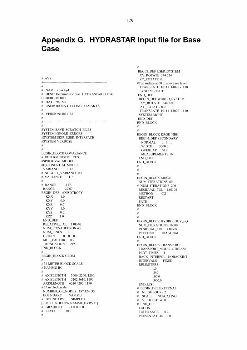
129
Appendix G. HYDRASTAR Input file for BaseCase
# AVS
#----------------------------------------------------------
#
# NAME: cbas.hyd
# DESC: Deterministic case HYDRASTAR LOCAL
CEBERG MODEL
# DATE: 980227
# USER: BJORN GYLLING, KEMAKTA
#
# VERSION: HS 1.7.1
#
#----------------------------------------------------------
#
SYSTEM SAVE_SCRATCH_FILES
SYSTEM IGNORE_ERRORS
#SYSTEM SKIP_USER_INTERFACE
#SYSTEM VERBOSE
#
#
BEGIN_BLOCK COVARIANCE
# DETERMINISTIC YES
#SPHERIVAL MODEL
#EXPONENTIAL MODEL
VARIANCE 1.12
# NUGGET_VARIANCE 0.5
# VARIANCE 1.7
#
# RANGE -117.
RANGE -22.67
BEGIN_DEF ANISOTROPY
KXX 1.0
KXY 0.0
KXZ 0.0
KYY 1.0
KYZ 0.0
KZZ 1.0
END_DEF
RELATIVE_TOL 1.0E-02
NUM_ICOSAHEDRON 40
NUM_LINES 0
ORIGIN 0.0 0.0 0.0
MUL_FACTOR 0.2
TRUNCATION 999.
END_BLOCK
#
BEGIN_BLOCK GEOM
#
# 34 METER BLOCK SCALE
# NAMMU BC
#
# AXISLENGTH 3000. 2200. 1200.
# AXISLENGTH 5202 5610. 1190.
AXISLENGTH 6510 4290. 1190.
# 35 m block scale
NUMBER_OF_NODES 187 124 35
BOUNDARY NAMMU
# BOUNDARY SIMPLE #
[SIMPLE,NOFLOW,NAMMU,HYRV11]
# GRADIENT -1.0 0.0 0.0
# LEVEL 10.0
#
#
BEGIN_DEF USER_SYSTEM
XY_ROTATE 344.524
ZY_ROTATE 0.
#Top surface at 60 m above sea level
TRANSLATE 10111 14020 -1130
SYSTEM RIGHT
END_DEF
BEGIN_DEF WORLD_SYSTEM
XY_ROTATE 344.524
ZY_ROTATE 0.0
TRANSLATE 10111 14020 -1130
SYSTEM RIGHT
END_DEF
END_BLOCK
#
#
BEGIN_BLOCK KRGE_NBH
BEGIN_DEF SECONDARY
NORMAL 0. 0. 1.
WIDTH 3000.0
OVERLAP 50.0
MEASUREMENTS 16
END_DEF
END_BLOCK
#
#
#
BEGIN_BLOCK KRIGE
NUM_ITERATIONS 60
# NUM_ITERATIONS 200
RESIDUAL_TOL 1.0E-02
METHOD CG
RESTART
PATH .
END_BLOCK
#
#
#
BEGIN_BLOCK HYDROLOGY_EQ
NUM_ITERATIONS 16000
RESIDUAL_TOL 1.0E-09
PRECOND DIAGONAL
END_BLOCK
#
BEGIN_BLOCK TRANSPORT
TRANSPORT_MODEL STREAM
PLOT_TIMES 1
BACK_INTERPOL NOBACKINT
INTERVALS FIXED
DELIMITERS
1.0
10.0
100.0
1000.0
END_LIST
# BEGIN_DEF EXTERNAL
# NEIGHBOURS 2
# SCALE NOSCALING
# VEL1DIST 40.0
# END_DEF
LOGON
TOLERANCE 0.2
PRESENTATION 0.0
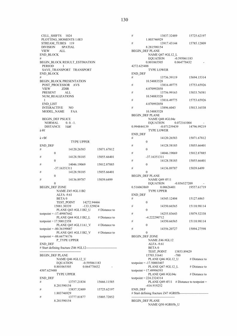
130
CELL_SHIFTS 1024
PLOTTING_MOMENTS 1.0E5
STREAM_TUBES 119
DIVISION SPATIAL
VIEW ALL
END_BLOCK
#
BEGIN_BLOCK RESULT_ESTIMATION
PERIOD 1
SAVE_TRANSPORT TRANSPORT
END_BLOCK
#
BEGIN_BLOCK PRESENTATION
POST_PROCESSOR AVS
VIEW ZDIR
PRESENT ALL
NUM_REALIZATIONS
1
END_LIST
INTERACTIVE NO
MODEL_NAME FAA
BEGIN_DEF PSLICE
NORMAL 0. 0. -1.
DISTANCE 1üâ€
à €€
à v$€
TYPE UPPER
END_DEF
# 14120.26583 15071.67812
0
# 14128.58185 15055.66401
0
# 14046.19069 15012.87885
-37.16351311
# 14128.58185 15055.66401
0
# 14136.89787 15039.6499
0
BEGIN_DEF ZONE
NAME Z45 #GL11B2
ALFA -9.61
BETA 0
TEST_POINT 14272.94466
15081.30339 -133.329834
PLANE Q43 #GL11B2_U # Distance to
testpoint = -17.49987642
PLANE Q44 #GL11B2_L # Distance to
testpoint = 17.50012358
PLANE Q45 #GL11A1_V # Distance to
testpoint = -80.36199087
PLANE Q41 #GL11B2_V # Distance to
testpoint = -88.66774176
P_TYPE UPPER
END_DEF
# Start defining fracture Z46 #GL12-----------------------------
---------------------------------------
BEGIN_DEF PLANE
NAME Q46 #GL12_U
EQUATION -0.595061183
0.801065505 0.064778432 -
4307.625488
TYPE UPPER
END_DEF
# 13757.21834 15666.11585
8.281590154
# 13837.32489 15725.62197
1.803746929
# 13777.81877 15805.72852
8.281590154
# 13837.32489 15725.62197
1.803746929
# 13917.43144 15785.12809
8.281590154
BEGIN_DEF PLANE
NAME Q47 #GL12_L
EQUATION -0.595061183
0.801065505 0.064778432 -
4272.625488
TYPE LOWER
END_DEF
# 13736.39119 15694.15314
10.54883528
# 13816.49775 15753.65926
4.070992058
# 13756.99163 15833.76581
10.54883528
# 13816.49775 15753.65926
4.070992058
# 13896.6043 15813.16538
10.54883528
BEGIN_DEF PLANE
NAME Q48 #GL04e
EQUATION 0.072161004 -
0.994844139 -0.071259439 14796.99219
TYPE LOWER
END_DEF
# 14120.26583 15071.67812
0
# 14128.58185 15055.66401
0
# 14046.19069 15012.87885
-37.16351311
# 14128.58185 15055.66401
0
# 14136.89787 15039.6499
0
BEGIN_DEF PLANE
NAME Q49 #F11
EQUATION -0.856527209 -
0.516063869 0.00626401 19557.61719
TYPE UPPER
END_DEF
# 14345.12404 15127.6863
0
# 14350.66565 15110.98114
0
# 14255.83643 15079.52338
-4.222290712
# 14350.66565 15110.98114
0
# 14356.20727 15094.27598
0
BEGIN_DEF ZONE
NAME Z46 #GL12
ALFA -9.61
BETA 0
TEST_POINT 13853.89429
15703.31641 -700
PLANE Q46 #GL12_U # Distance to
testpoint = -17.50003407
PLANE Q47 #GL12_L # Distance to
testpoint = 17.49996593
PLANE Q48 #GL04e # Distance to
testpoint = 224.2324314
PLANE Q49 #F11 # Distance to testpoint =
-416.919252
END_DEF
# Start defining fracture Z47 #GR05b---------------------------
-----------------------------------------
BEGIN_DEF PLANE
NAME Q50 #GR05b_U

131
EQUATION 0.87014246
0.492800236 0 -21235.6543
TYPE UPPER
END_DEF
# 16249.49272 14328.89184
0
# 16298.77275 14241.8776
0
# 16385.78699 14291.15762
0
# 16298.77275 14241.8776
0
# 16348.05277 14154.86335
0
BEGIN_DEF PLANE
NAME Q51 #GR05b_L
EQUATION 0.87014246
0.492800236 0 -21200.6543
TYPE LOWER
END_DEF
# 16279.94771 14346.13985
0
# 16329.22773 14259.1256
0
# 16416.24198 14308.40563
0
# 16329.22773 14259.1256
0
# 16378.50776 14172.11136
0
BEGIN_DEF PLANE
NAME Q52 #GR05a_V
EQUATION -0.285761391
0.958300802 0 -7546.57515
TYPE LOWER
END_DEF
# 17063.20533 12963.13267
0
# 17045.99944 12958.00194
0
# 17017.4233 13053.83202
0
# 17045.99944 12958.00194
0
# 17028.79355 12952.87121
0
BEGIN_DEF PLANE
NAME Q53 #F12
EQUATION -0.901027381
0.433762193 0 7297.842773
TYPE UPPER
END_DEF
# 14345.12404 15127.6863
0
# 14350.66565 15110.98114
0
# 14255.83643 15079.52338
-4.222290712
# 14350.66565 15110.98114
0
# 14356.20727 15094.27598
0
BEGIN_DEF ZONE
NAME Z47 #GR05b
ALFA -9.61
BETA 0
TEST_POINT 16314 14250.50146
-700
PLANE Q50 #GR05b_U # Distance to
testpoint = -17.49972516
PLANE Q51 #GR05b_L # Distance to
testpoint = 17.50027484
PLANE Q52 #GR05a_V # Distance to
testpoint = 1447.78051
PLANE Q53 #F12 # Distance to testpoint =
-1220.189164
END_DEF
# Start defining fracture Z48 #GR14a---------------------------
-----------------------------------------
BEGIN_DEF PLANE
NAME Q54 #GR14a_U
EQUATION 0.97285372
0.231420875 0 -13868.23242
TYPE UPPER
END_DEF
# 10474.11329 15743.83659
0
# 10497.25538 15646.55122
0
# 10594.54075 15669.69331
0
# 10497.25538 15646.55122
0
# 10520.39747 15549.26585
0
BEGIN_DEF PLANE
NAME Q55 #GR14a_L
EQUATION 0.97285372
0.231420875 0 -13833.23242
TYPE LOWER
END_DEF
# 10508.16317 15751.93632
0
# 10531.30526 15654.65095
0
# 10628.59063 15677.79304
0
# 10531.30526 15654.65095
0
# 10554.44735 15557.36558
0
BEGIN_DEF PLANE
NAME Q56 #GR15b
EQUATION -0.266835183 -
0.963742197 0 16286.76074
TYPE UPPER
END_DEF
# 17063.20533 12963.13267
0
# 17045.99944 12958.00194
0
# 17017.4233 13053.83202
0
# 17045.99944 12958.00194
0
# 17028.79355 12952.87121
0
BEGIN_DEF PLANE
NAME Q57 #GR40a_V
EQUATION 0.237961405 -
0.971274611 0 14528.07994
TYPE LOWER
END_DEF
# 10073.9946 17425.86665
0
# 10090.99229 17430.03107
0
# 10114.78843 17332.90361
0
# 10090.99229 17430.03107
0
# 10107.98998 17434.19549
0
BEGIN_DEF ZONE

132
NAME Z48 #GR14a
ALFA -9.61
BETA 0
TEST_POINT 10514.28027
15650.60107 -700
PLANE Q54 #GR14a_U # Distance to
testpoint = -17.49995422
PLANE Q55 #GR14a_L # Distance to
testpoint = 17.50004578
PLANE Q56 #GR15b # Distance to
testpoint = -1601.963814
PLANE Q57 #GR40a_V # Distance to
testpoint = 1829.041384
END_DEF
# Start defining fracture Z49 #GR15b---------------------------
-----------------------------------------
BEGIN_DEF PLANE
NAME Q58 #GR15b_U
EQUATION -0.266835183 -
0.963742197 0 16269.26074
TYPE UPPER
END_DEF
# 12613.86386 13425.20622
0
# 12517.48964 13451.88974
0
# 12490.80612 13355.51552
0
# 12517.48964 13451.88974
0
# 12421.11542 13478.57326
0
BEGIN_DEF PLANE
NAME Q59 #GR15b_L
EQUATION -0.266835183 -
0.963742197 0 16304.26074
TYPE LOWER
END_DEF
# 12604.52463 13391.47524
0
# 12508.15041 13418.15876
0
# 12481.46689 13321.78454
0
# 12508.15041 13418.15876
0
# 12411.77619 13444.84228
0
BEGIN_DEF PLANE
NAME Q60 #GR05a
EQUATION 0.997933686
0.064252369 0 -17843.35938
TYPE UPPER
END_DEF
# 17063.20533 12963.13267
0
# 17045.99944 12958.00194
0
# 17017.4233 13053.83202
0
# 17045.99944 12958.00194
0
# 17028.79355 12952.87121
0
BEGIN_DEF PLANE
NAME Q61 #GR15a_V
EQUATION 0.936133433 -
0.351644985 0 -2251.578187
TYPE LOWER
END_DEF
# 7922.456069 14687.81877
0
# 7928.63443 14704.26653
0
# 8022.247773 14669.10203
0
# 7928.63443 14704.26653
0
# 7934.812791 14720.71428
0
BEGIN_DEF ZONE
NAME Z49 #GR15b
ALFA -9.61
BETA 0
TEST_POINT 12512.82007
13435.02441 -700
PLANE Q58 #GR15b_U # Distance to
testpoint = -17.49982906
PLANE Q59 #GR15b_L # Distance to
testpoint = 17.50017094
PLANE Q60 #GR05a # Distance to
testpoint = -4493.162577
PLANE Q61 #GR15a_V # Distance to
testpoint = 4737.732064
END_DEF
# Start defining fracture Z50 #GR79-GL07---------------------
-----------------------------------------------
BEGIN_DEF PLANE
NAME Q62 #GR79-GL07_U
EQUATION 0.87871033
0.422993124 0.221235037 -
17899.57422
TYPE UPPER
END_DEF
# 14572.07708 12678.56338
52.51332888
# 14614.3764 12590.69234
30.38982519
# 14702.24743 12632.99166
52.51332888
# 14614.3764 12590.69234
30.38982519
# 14656.67571 12502.82131
52.51332888
BEGIN_DEF PLANE
NAME Q63 #GR79-GL07_L
EQUATION 0.87871033
0.422993124 0.221235037 -
17864.57422
TYPE LOWER
END_DEF
# 14602.83195 12693.36814
60.2565553
# 14645.13126 12605.4971
38.13305161
# 14733.00229 12647.79642
60.2565553
# 14645.13126 12605.4971
38.13305161
# 14687.43057 12517.62607
60.2565553
BEGIN_DEF PLANE
NAME Q64 #F16
EQUATION 0.869803071 -
0.493399024 0 -8405.542969
TYPE UPPER
END_DEF
# 7922.456069 14687.81877
0
# 7928.63443 14704.26653
0
# 8022.247773 14669.10203
0
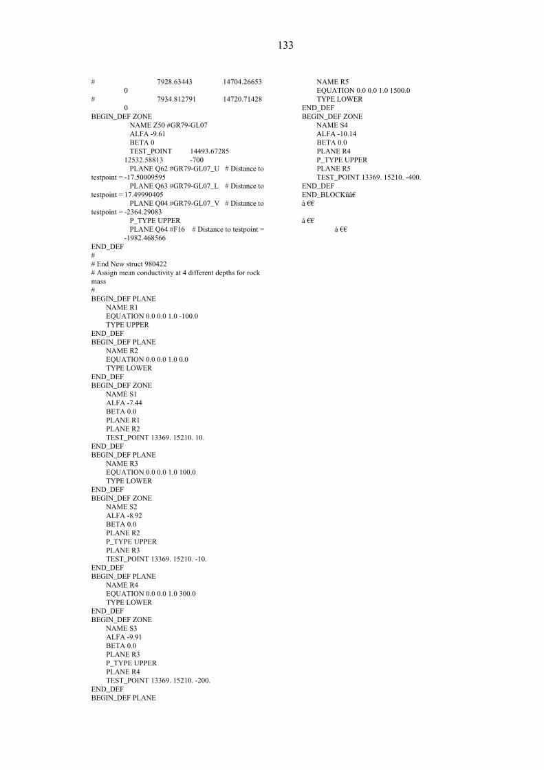
133
# 7928.63443 14704.26653
0
# 7934.812791 14720.71428
0
BEGIN_DEF ZONE
NAME Z50 #GR79-GL07
ALFA -9.61
BETA 0
TEST_POINT 14493.67285
12532.58813 -700
PLANE Q62 #GR79-GL07_U # Distance to
testpoint = -17.50009595
PLANE Q63 #GR79-GL07_L # Distance to
testpoint = 17.49990405
PLANE Q04 #GR79-GL07_V # Distance to
testpoint = -2364.29083
P_TYPE UPPER
PLANE Q64 #F16 # Distance to testpoint =
-1982.468566
END_DEF
#
# End New struct 980422
# Assign mean conductivity at 4 different depths for rock
mass
#
BEGIN_DEF PLANE
NAME R1
EQUATION 0.0 0.0 1.0 -100.0
TYPE UPPER
END_DEF
BEGIN_DEF PLANE
NAME R2
EQUATION 0.0 0.0 1.0 0.0
TYPE LOWER
END_DEF
BEGIN_DEF ZONE
NAME S1
ALFA -7.44
BETA 0.0
PLANE R1
PLANE R2
TEST_POINT 13369. 15210. 10.
END_DEF
BEGIN_DEF PLANE
NAME R3
EQUATION 0.0 0.0 1.0 100.0
TYPE LOWER
END_DEF
BEGIN_DEF ZONE
NAME S2
ALFA -8.92
BETA 0.0
PLANE R2
P_TYPE UPPER
PLANE R3
TEST_POINT 13369. 15210. -10.
END_DEF
BEGIN_DEF PLANE
NAME R4
EQUATION 0.0 0.0 1.0 300.0
TYPE LOWER
END_DEF
BEGIN_DEF ZONE
NAME S3
ALFA -9.91
BETA 0.0
PLANE R3
P_TYPE UPPER
PLANE R4
TEST_POINT 13369. 15210. -200.
END_DEF
BEGIN_DEF PLANE
NAME R5
EQUATION 0.0 0.0 1.0 1500.0
TYPE LOWER
END_DEF
BEGIN_DEF ZONE
NAME S4
ALFA -10.14
BETA 0.0
PLANE R4
P_TYPE UPPER
PLANE R5
TEST_POINT 13369. 15210. -400.
END_DEF
END_BLOCKüâ€
à €€
à €€
à €€

135
Appendix H. Coordinate Transforms
The Ceberg simulations use a local coordinate system based on a translation (off-set) of
the Swedish National grid (the RAK system). This means that all input data in the form
of e.g. stream tube starting positions and fracture zones must be defined for the local
system. The model is set up in the local system with the origin for the model cube at
(10111, 14020, -1190). The HYDRASTAR modelling terms “user system” and “world
system” are defined using that point in the local system. The HYDRASTAR “cube
system” is rotated 15.48 degrees clock-wise in relation to the local system. The used
definitions of coordinate systems give output data for e.g. exit locations, which could be
extracted from the lines_<real>.hyp files, in the local system (that is, the rotation of the
cube system is made internally in HYDRASTAR).
The Ceberg local coordinate system used in the groundwater simulations uses a
translation of 1,650,000 m and 7,030,000 m from RAK grid coordinates, in east and
north, respectively (Boghammar et al., 1997). The coordinate systems for Ceberg are
right-hand-rule with X towards east and Y towards north. The Z-direction is given in
metres above sea level (masl). To translate the modelling coordinates to RAK, the
following equations have been used:
XRAK = XOff-set + XC
YRAK = YOff-set +YC
where XRAK and YRAK stand for east and north, respectively; XC and YC are Ceberg
modelling coordinates; XOff-set = 1 650 000; and YOff-set = 7 030 000.