Groundwater Modelling Report Modelling Report 500-074 Groundwater Modelling Report_Final_20 August 2013 PAGE i Groundwater Modelling Report August 2013 This document records technical

Groundwater Modelling Report

500-074 Groundwater Modelling Report_Final_20 August 2013 PAGE i


August 2013

This document records technical and factual information used to support the NZTA's Assessment of Environmental Effects for the Pūhoi to Warkworth Project. It has been supplied to the Environmental Protection Authority by the NZTA in response to a section 149(2) Resource Management Act 1991 request. This document did not form part of the NZTA's application for the Project, which was lodged on 30 August 2013.


500-074 Groundwater Modelling Report_Final_20 August 2013 PAGE i

Pūhoi to Warkworth

Document title: Groundwater Modelling Report

Version: Final

Date: 20 August 2013

Prepared by: Jon Williamson

Approved by: Tony Innes

File name: 500-074 Groundwater Modelling Report_Final_20 August 2013

Further North Alliance Office

Level 2, Carlaw Park

12-16 Nicholls Lane

Parnell, Auckland

New Zealand

Tel: 0800 P2W NZTA (0800 729 6982)

Email: [email protected]

Tel: www.nzta.govt.nz/projects/Puhoi-wellsford

LIMITATION: This document has been prepared by the Further North Alliance (FNA) in accordance with the identified scope and for the benefit of the New Zealand Transport Agency. No liability is accepted by either of these entities (or their employees or sub-consultants) with respect to the use of this document by any other person. This disclaimer shall apply notwithstanding that this document may be made available to other persons for an application for permission or approval or to fulfill a legal requirement.


500-074 Groundwater Modelling Report_Final_20 August 2013 PAGE ii

Glossary of abbreviations Abbreviation Definition

km Kilometers

km2 Square kilometers

L/s Litres per second

mAMSL Metres Above Mean Sea Level

m Metres

m/s Metres per second

mRL Metres Reduced Level

NZTA NZ Transport Agency

RMS Root mean square

RoNS Roads of National Significance


500-074 Groundwater Modelling Report_Final_20 August 2013 PAGE iii

Glossary of defined terms Term Definition

Allochthon A large block of rock which has been moved from its original site of formation, usually by low angle thrust faulting.

Anisotropy Anisotropy in an aquifer occurs when there is a difference in conductivity in two different directions. Whenever there is a difference in conductivity, water prefers to travel along the path with least resistance. In other words, water travels preferentially along the direction of higher conductivity.

Auckland Council The unitary authority that replaced eight councils in the Auckland Region as of 1 November 2010.

Bore Any hole (typically cylindrical) that has been constructed to provide access to groundwater (for example, for monitoring of ground or groundwater conditions, taking of groundwater or the discharge of stormwater).

Drawdown Drawdown is the reduction in groundwater level resulting from any form of development or activity

Ephemeral Streams that dry up intermittently during drought periods.

Groundwater Natural water contained within soil and rock formations below the surface of the ground.

Hydraulic conductivity The ability of an aquifer material to transmit water, measured as the flow rate of water through a cross section of 1m2 under a unit hydraulic gradient. Hydraulic conductivity is typically reported in units of m/d or m/s.

Perennial Stream or river with continuous flow all year round.

Permeability The ability of a porous material to allow fluids to pass through it.

Project Pūhoi to Warkworth section of the Ara Tūhono Pūhoi to Wellsford Road of National Significance Project.

Specific yield The quantity of water yielded or taken into storage under gravity by a unit change in water level. Specific yield is expressed either as a ratio or as a percentage of the volume of the aquifer, with values typically residing between 0.01 and 0.3 or 1% to 30%.

Wetland Natural feature of the landscape that is saturated by surface or groundwater at a frequency and duration sufficient to support vegetation adapted to wet conditions.


500-074 Groundwater Modelling Report_Final_20 August 2013 PAGE iv

Contents 1. Introduction ............................................................................................................... 12. Model setup ................................................................................................................ 22.1 Model domain ................................................................................................................ 22.2 Areal discretisation ......................................................................................................... 22.3 Vertical refinement ......................................................................................................... 32.4 Boundary conditions ....................................................................................................... 43. Model calibration ........................................................................................................ 64. Sensitivity analysis ..................................................................................................... 95. Predictive analysis .................................................................................................... 115.1 Drawdown extent and impacts........................................................................................115.2 Stream flow reduction ...................................................................................................115.3 Cut seepage rates .........................................................................................................126. Conclusions .............................................................................................................. 14


500-074 Groundwater Modelling Report_Final_20 August 2013 PAGE 1

1. Introduction

This Report supplements the Hydrogeology Assessment Report prepared for the New Zealand Transport Agency (NZTA). The Hydrogeology Assessment Report provides an assessment of the environmental effects associated with groundwater, arising from the implementation of the Pūhoi to Warkworth section (the Project) of the Ara Tūhono Pūhoi to Wellsford Road of National Significance Project. The Hydrogeology Assessment Report informs the Assessment of Environmental Effects (AEE) and supports the resource consent applications and Notices of Requirement for the Project. This report does not form part of the application documentation for the Project.

A groundwater numerical model is a simulation tool that can be used to assist in the understanding of groundwater flow dynamics and impacts under natural and developed conditions.

In its simplest application, a groundwater model facilitates the combination of hydrogeological field data collected from an area into a single simulation interface to provide a level of verification of the collected data and an understanding of data gaps (e.g. probable groundwater levels in unmonitored areas). The application and accuracy of any numerical model depends on the quantity and quality of input data available for use in the model’s development.

For the Project, a fully three dimensional numerical model was developed using the Wasy-DHI FeFlow finite element groundwater modelling platform. The model was developed to quantify:

1) groundwater levels and flow directions through the designation areas and adjoining areas;

2) groundwater depressurisation adjacent to cuts and excavations;

3) groundwater seepage to cuts and excavations;

4) reduction in groundwater baseflows to streams, wetlands and rivers.

There are a number of key features of an appropriate model. These are described in the following sections.



2. Model setup

2.1 Model domain

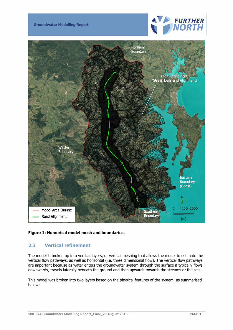
The model domain comprises an area encompassing 164km2, extending from Johnstone’s Hill in the south to 2 km north of Warkworth, a distance of approximately 18km, with an west to east width of between 3-6km (Figure 1). The placement of the boundaries was selected so as to capture the areas most likely to have a role in governing the hydrogeology of the proposed designation and potential impact areas.

In this model, northern, western and southern boundaries have been defined along topographic ridges approximately 2km away from the designation. Defining boundaries on ridges negates potential errors in assignment of model side fluxes (incoming or exiting water) because ridges act as natural groundwater flow divisions, meaning in and outward flows do not need to be considered in the model at these locations.

The eastern boundary of the system runs approximately parallel to the proposed designation along the coast at a distance of between 3 to 6km from the proposed alignment. The coast acts as a natural flow sink, draining excess groundwater from the system.

2.2 Areal discretisation

The model’s mesh discretisation (setup) provides a high level of accuracy in areas of most importance to the Project. This was achieved through strategic placement or alignment of the model nodes and variable mesh granularity, as shown in Figure 1.

Node alignment focussed on key features of the landscape that govern hydrogeological processes under both the natural and proposed development scenarios, such as streams, rivers, existing bores and the proposed road alignment.

Mesh granularity optimises accuracy versus runtime efficiency, hence more intense mesh spacing was implemented along the proposed highway alignment and lower intensity mesh (increased spacing) was implemented in distal areas of the model away from the highway alignment.

The width sizes of the model mesh varies from approximately 3m along the alignment, to 10-15m in the general refinement areas along water courses, to up to 500m in the distal low focus areas.



Figure 1: Numerical model mesh and boundaries.

2.3 Vertical refinement

The model is broken up into vertical layers, or vertical meshing that allows the model to estimate the vertical flow pathways, as well as horizontal (i.e. three dimensional flow). The vertical flow pathways are important because as water enters the groundwater system through the surface it typically flows downwards, travels laterally beneath the ground and then upwards towards the streams or the sea.

This model was broken into two layers based on the physical features of the system, as summarised below:

Southern Boundary



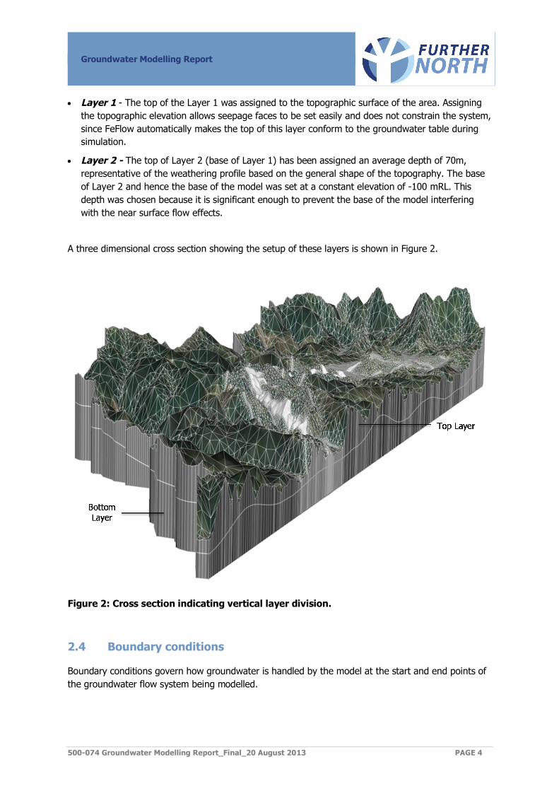
· Layer 1 - The top of the Layer 1 was assigned to the topographic surface of the area. Assigning the topographic elevation allows seepage faces to be set easily and does not constrain the system, since FeFlow automatically makes the top of this layer conform to the groundwater table during simulation.

· Layer 2 - The top of Layer 2 (base of Layer 1) has been assigned an average depth of 70m, representative of the weathering profile based on the general shape of the topography. The base of Layer 2 and hence the base of the model was set at a constant elevation of -100 mRL. This depth was chosen because it is significant enough to prevent the base of the model interfering with the near surface flow effects.

A three dimensional cross section showing the setup of these layers is shown in Figure 2.

Figure 2: Cross section indicating vertical layer division.

2.4 Boundary conditions

Boundary conditions govern how groundwater is handled by the model at the start and end points of the groundwater flow system being modelled.



Recharge Boundary

Rainfall recharge is the only source of input water in this model. It is applied over the entire surface of the area as a constant inflow, representing the proportion of rainfall that is not lost through evaporation or surface runoff.

No Flow Boundaries

There are two main groups of no flow boundaries in this system. It was mentioned previously that the northwest and south boundaries were defined along ridges, which act as flow divides. Since no flow crosses these divides, these boundaries were assigned as no flow conditions. The base of the model has also been defined as a no flow boundary, as the significant depth (-100 mRL) of the model base means it will not have any significant influence on near surface flow dynamics.

Drainage Boundaries

There are two sets of drainage boundaries in this system:

· Eastern boundary - running along the coast is assigned drainage boundaries at sea level representing drainage into the sea.

· Streams - in the system are represented by defining seepage faces across the ground surface. This means that if the water table intercepts the topography of the system, water will be drained at the low lying points, which in this case are the streams, wetlands and rivers.



3. Model calibration

The model has been calibrated to the physical observations of the system. These observations consist of the water levels obtained from groundwater bores throughout the model area. Calibration of the model to these levels involved altering both the hydraulic conductivity of the geological formations in the area and the rainfall recharge at the surface. Other hydraulic parameters such as specific storage and specific yield are used in transient model calibration; however these parameters have not been used here, since this is a steady state model only.

The calibration process undertaken comprised two phases of work:

1) Preliminary Calibration - A preliminary calibration to the observed regional water levels was performed by breaking the model up into the three main geology types based on the surface geology map; Waitemata Group, Northern Allochthon and alluvium. The hydraulic parameters of these units as well as the rainfall recharge rate were varied until most of the water levels in the system were roughly matched to observed groundwater levels. This calibration resulted in the general hydraulic conductivity values shown in Table 1, together with a mean annual rainfall recharge estimate of 50 mm/annum (approximately 3.3% of annual rainfall). This estimate is consistent with other studies and Auckland Council indicate recharge in the Waitemata group materials (which comprise the majority of the geology in the model area) typically range from 2 to 4% of mean annual rainfall (pers. com., Kelsey, 2013 working on behalf of Auckland Council).

Table 1: Calibrated hydraulic conductivities – general calibration.

Material Hydraulic Conductivity (m/s) Vertical Anisotropy

Alluvium 1.0x10-6 0.1

Northern Allochthon 5.0x10-8 0.1

Waitemata Group (General) 1.0x10-7 0.1

Waitemata Group (Western Section) 2.5x10-8 0.1

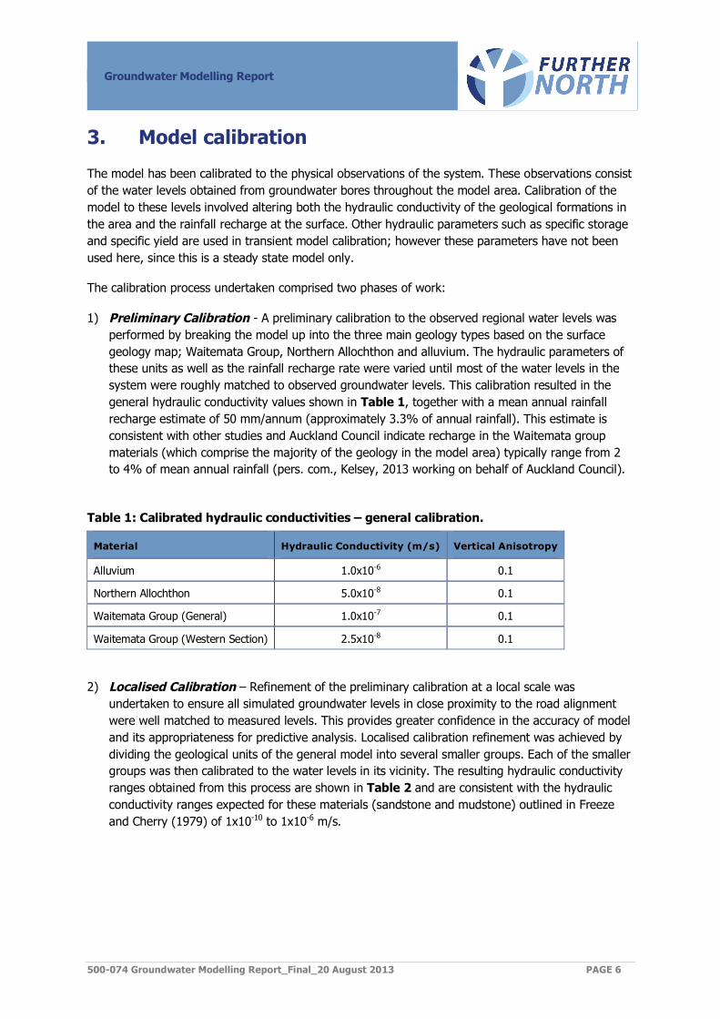
2) Localised Calibration – Refinement of the preliminary calibration at a local scale was undertaken to ensure all simulated groundwater levels in close proximity to the road alignment were well matched to measured levels. This provides greater confidence in the accuracy of model and its appropriateness for predictive analysis. Localised calibration refinement was achieved by dividing the geological units of the general model into several smaller groups. Each of the smaller groups was then calibrated to the water levels in its vicinity. The resulting hydraulic conductivity ranges obtained from this process are shown in Table 2 and are consistent with the hydraulic conductivity ranges expected for these materials (sandstone and mudstone) outlined in Freeze and Cherry (1979) of 1x10-10 to 1x10-6 m/s.



Table 2: Calibrated hydraulic conductivities – localised calibration.

Material

Hydraulic Conductivity

Vertical Anisotropy Max (m/s) Min (m/s)

Alluvium 1.0x10-6 1.0x10-6 0.1

Northern Allocthon 5.0x10-8 5.0x10-8 0.1

Waitemata Group 7.0x10-7 1.2x10-8 0.1

Plots of the localised variation in hydraulic conductivity for the two model layers are shown in Figure 3.

Figure 3: Calibrated hydraulic conductivities.

Layer 1 Layer 2



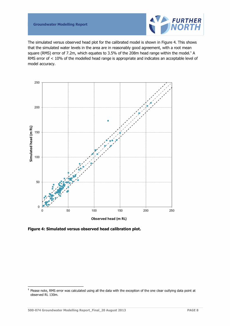
The simulated versus observed head plot for the calibrated model is shown in Figure 4. This shows that the simulated water levels in the area are in reasonably good agreement, with a root mean square (RMS) error of 7.2m, which equates to 3.5% of the 208m head range within the model.1 A RMS error of < 10% of the modelled head range is appropriate and indicates an acceptable level of model accuracy.

Figure 4: Simulated versus observed head calibration plot.

1 Please note, RMS error was calculated using all the data with the exception of the one clear outlying data point at

observed RL 130m.

0

50

100

150

200

250

0 50 100 150 200 250

Sim

ulat

ed h

ead

(m R

L)

Observed head (m RL)



4. Sensitivity analysis

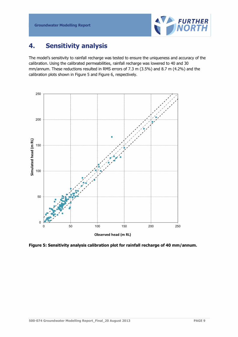
The model’s sensitivity to rainfall recharge was tested to ensure the uniqueness and accuracy of the calibration. Using the calibrated permeabilities, rainfall recharge was lowered to 40 and 30 mm/annum. These reductions resulted in RMS errors of 7.3 m (3.5%) and 8.7 m (4.2%) and the calibration plots shown in Figure 5 and Figure 6, respectively.

Figure 5: Sensitivity analysis calibration plot for rainfall recharge of 40 mm/annum.

0

50

100

150

200

250

0 50 100 150 200 250

Sim

ulat

ed h

ead

(m R

L)




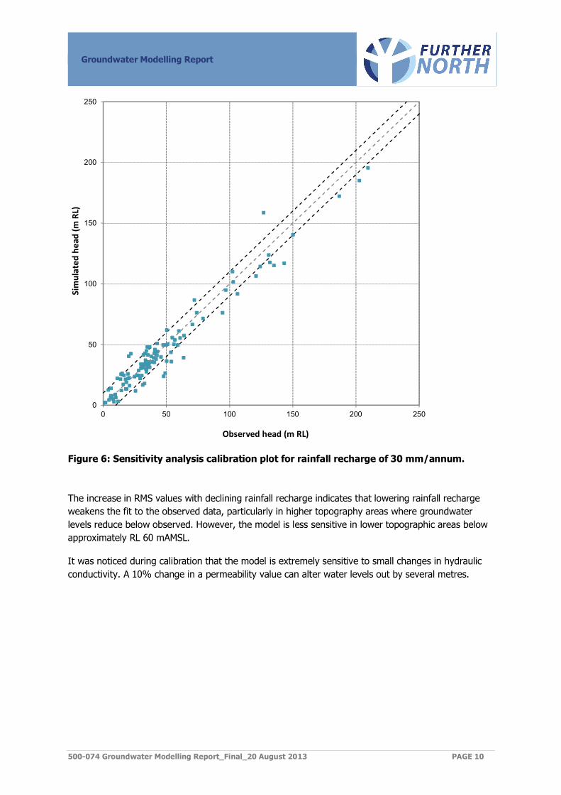
Figure 6: Sensitivity analysis calibration plot for rainfall recharge of 30 mm/annum.

The increase in RMS values with declining rainfall recharge indicates that lowering rainfall recharge weakens the fit to the observed data, particularly in higher topography areas where groundwater levels reduce below observed. However, the model is less sensitive in lower topographic areas below approximately RL 60 mAMSL.

It was noticed during calibration that the model is extremely sensitive to small changes in hydraulic conductivity. A 10% change in a permeability value can alter water levels out by several metres.

0

50

100

150

200

250

0 50 100 150 200 250

Sim

ulat

ed h

ead

(m R

L)




5. Predictive analysis

The model was used in steady-state mode to perform predictive analysis of the impacts of the indicative alignment, focussing on the following impacts:

· Extent of drawdown from cuts; and

· Depletion of groundwater flow to surface water bodies (wetlands, streams and rivers).

The top surface of the model was lowered to represent the elevation of the proposed highway cuts. This constrains groundwater level to the near the invert of the cut and forces any intercepted groundwater to be drained.

The following sections describe the comparison between groundwater levels and groundwater dependent flows of the calibrated model and the predictive model.

5.1 Drawdown extent and impacts

The extent of drawdown2 defines the area within which potential impacts are most likely to be experienced, and is shown in Drawings ES-101 to ES-117. From these figures, which show drawdown contours of 0.1m (the smallest drawdown level that can be practically measured) to a maximum of 35m, several observations can be made:

1) All the measurable drawdown is contained within a 700m radius of the indicative alignment, meaning that any use of groundwater outside this radius is unlikely to be affected by the cuts;

2) Drawdowns of 5m or more are observed at almost all major cuts along the alignment, at radii of up to 160m from these cuts.

5.2 Stream flow reduction

The model was used to analyse depletion of groundwater input to streams (stream flow depletion). Stream flow depletion is important because a reduction in groundwater inputs (baseflow) may reduce habitat quality depending on the scale of reduction. This impact is only of significance during low flow events, as during these times the proportion of water in a stream is predominately groundwater. During high to flood flows, the volume of the surface water component in stream flow is exponentially higher than the groundwater component.

Only streams considered to be perennial3 by the Further North hydrologists were selected for analysis. Groundwater discharge to each selected stream was simulated under natural state conditions with the calibrated model. This was also simulated using the predictive model with the cuts included, and baseflow reduction calculated for each stream.

The stream depletion analysis undertaken represents an upper limit on the impact expected because of the following assumptions:

2 Drawdown in the context of this project is the difference between the simulated natural groundwater conditions and

those following construction of the proposed highway cuts. 3 Perennial streams flow year round, whereas ephemeral streams dry up intermittently during drought periods.



· Groundwater seepages at the cuts are not channelled back into nearby surface water courses. However, in practice any groundwater seepages or diversions will be routed through the Project’s stormwater system; and

· Streams assessed included only perennial streams located either crossing or immediately adjacent to the indicative alignment, which means that any impacts would progressively lessen with distance downstream from the alignment because of the additional catchment contributions.

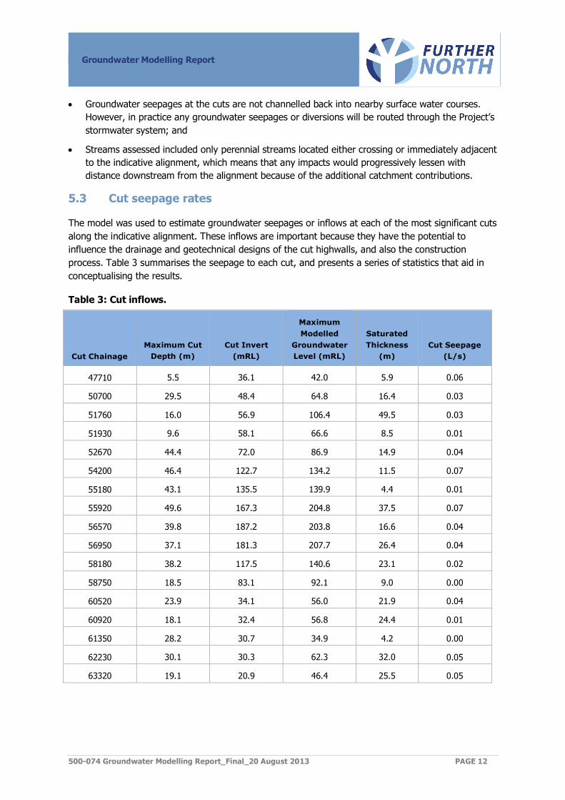
5.3 Cut seepage rates

The model was used to estimate groundwater seepages or inflows at each of the most significant cuts along the indicative alignment. These inflows are important because they have the potential to influence the drainage and geotechnical designs of the cut highwalls, and also the construction process. Table 3 summarises the seepage to each cut, and presents a series of statistics that aid in conceptualising the results.

Table 3: Cut inflows.

Cut Chainage Maximum Cut

Depth (m) Cut Invert

(mRL)

Maximum Modelled

Groundwater Level (mRL)

Saturated Thickness

(m) Cut Seepage

(L/s)

47710 5.5 36.1 42.0 5.9 0.06

50700 29.5 48.4 64.8 16.4 0.03

51760 16.0 56.9 106.4 49.5 0.03

51930 9.6 58.1 66.6 8.5 0.01

52670 44.4 72.0 86.9 14.9 0.04

54200 46.4 122.7 134.2 11.5 0.07

55180 43.1 135.5 139.9 4.4 0.01

55920 49.6 167.3 204.8 37.5 0.07

56570 39.8 187.2 203.8 16.6 0.04

56950 37.1 181.3 207.7 26.4 0.04

58180 38.2 117.5 140.6 23.1 0.02

58750 18.5 83.1 92.1 9.0 0.00

60520 23.9 34.1 56.0 21.9 0.04

60920 18.1 32.4 56.8 24.4 0.01

61350 28.2 30.7 34.9 4.2 0.00

62230 30.1 30.3 62.3 32.0 0.05

63320 19.1 20.9 46.4 25.5 0.05



The key finding in Table 3 is as follows:

· All cuts have inflows of 0.1 L/s or less, which is a very small flow and is half that of a standard garden hose (0.2 L/s).

· These inflows are comparable to the flow reductions observed in the stream flow reduction analysis.



6. Conclusions

A numerical model of the Project area was constructed and calibrated to observed groundwater levels in the area. This calibrated model was used to assess the potential impacts anticipated to result from earth cuts or excavations required along the road alignment.

No groundwater impacts are expected in fill areas due to drainage engineering works that will prevent groundwater mounding (rise), hence this was not assessed with the groundwater model.

Drawdown contours from the cuts showed that drawdown impacts are unlikely to be felt further than 500m from the alignment given the low permeability of the materials in the area, hence groundwater users will not be impacted if outside this 700m radius.

Stream baseflow reductions were analysed and it was found that the reduction was small in absolute magnitude (L/s), but proportionately for some of the smaller streams, the baseflow reduction represented a large proportion of the flow at that point. In those cases, where stream flows have a large proportionate affect, the streams in question typically have very small naturally occurring baseflow rates (0.05 L/s or less) due to their small catchment size. Given the small magnitude of flow, these streams are more likely wet depressions or wet areas. The ecological significance of these is commented on in the Freshwater Ecology Assessment Report.

Groundwater seepages to the major cuts along the proposed alignment were analysed and found to have very low inflows of 0.1 L/s or less.

Documents

Groundwater Modelling Report Modelling Report 500-074 Groundwater Modelling Report_Final_20 August 2013 PAGE i Groundwater Modelling Report August 2013 This document records technical