Simulation and high-precision wavelength determination of

Applied Physics B - Lasers and Optics,DOI 10.1007/s00340-011-4391-9The original publication is available athttp://www.springerlink.com/content/u3311lvg67060665/

Simulation and high-precision wavelength determination of noisy 2D Fabry-Perotinterferometric rings for direct-detection Doppler lidar and laser spectroscopy

Markus C. Hirschberger and Gerhard Ehret

Deutsches Zentrum fur Luft- und Raumfahrt (DLR), Institutfur Physik der Atmosphare (IPA),Oberpfaffenhofen, Munchner Str. 20, 82234 Wessling, Germanye-mail:[email protected] , phone: 08153/28-2554 , fax: 08153/28-1271

Received: 28 July 2010 / Revised version: 13 December 2010

Abstract Doppler wind lidar (DWL) measurements by thefringe-imaging technique in front of aircrafts at flight speedrequire rapid processing of backscattered signals. We discussthe measurement principle to derive the 3D wind vector fromthree line-of-sight (LOS) measurements. Then we simulaterealistic fringe patterns of a Fabry-Perot-interferometer (FPI)on a 2D charge-coupled device (CCD) localized at the focalplane behind it, taking atmospheric and instrument proper-ties like scattering and noise into account. A laser at355 nmwith pulse energies of70mJ at 100Hz repetition rate and arange bin of only10m were assumed. This yields count ratesof 24 (13) million photons per pulse at56 (76)m distanceand8.5 km altitude, that are distributed on a CCD with up to960× 780 pixels without intensification and therefore gener-ate noisy pixel signals. We present two methods for the pre-cise determination of the radii, i.e. wavelengths, of thesesim-ulated FPI rings and show that both are suitable for eliminat-ing pixel noise from the output and coping with fringe broad-ening by Rayleigh scattering. One of them proves to reach theaccuracy necessary for LOS velocity measurements. A stan-dard deviation of2.5m

s including center determination can beachieved with only20 images to average. The bias is7m

s . Forexactly known ring centers, each can be even better than2m

s .The methods could also be useful for high-resolution laserspectroscopy.

PACS 42.68.Wt · 42.25.Hz· 95.55.Aq

1 Introduction

In atmospheric remote sensing, Doppler wind lidar (DWL)[1] is a commonly used tool for measuring the wavelengthor frequency shift of light backscattered from moving atmo-spheric molecules and aerosols, and thus extracting infor-mation about the wind speed and direction. Coherent [2–6]or incoherent detection methods were realized. Incoherent(direct-detection) DWL has three main categories: the edgeor double-edge (DE) technique [7–14], techniques based on

temperature stabilized iodine vapor cells as a frequency dis-criminator [15–17] and the fringe-imaging (FI) technique [18–22] . All three make use of instruments like Michelson [22] or(multiple) Fabry-Perot interferometers (FPI) [14,15,17,21],with lasers emitting at532 nm or even better at355 nm to ob-tain stronger signals from molecular backscattering. DE andFI techniques have been compared and analysed in [23,24].A FI-type FPI was the first one to be tested on aircraft [25,26] for wind speed measurements. FPIs are applied in scan-ning mode for plasma jet Rayleigh scattering measurementsto determine gas temperature and velocity profiles of plas-mas [27], in planar Doppler velocimetry [28] or, similar toour approach, in imaging mode to measure the flow proper-ties by Rayleigh scattering in a small supersonic wind tun-nel [29] via the locations of interference fringes [30] on atwo-dimensional (2D) charge-coupled device (CCD). Amongother Doppler lidar methods that use FPIs with 2D informa-tion are the image plane detector (IPD) for the Dynamics Ex-plorer spacecraft [31], which allows for circular-pixel ring-detection, and the circle-to-line interferometer opticalsystem(CLIO) [32,33], which uses a reflective cone to convert circu-lar fringes from a FPI into a linear series of spots on a CCD.A holographic circle-to-point converter for use with FPIs wasinvented, too [34]. We characterize a DWL that measures theDoppler shifts via FI in front of aircrafts using the angulardisplacement of Fabry-Perot fringes [35,36].

The main focus of the article is on two novel radii evalua-tion strategies including a center determination, that make useof the complete 2D information given on a CCD screen in thefocus behind a FPI, thus significantly reducing the noise ofsingle one-dimensional (1D) cuts through the 2D rings. Aftera calibration to relate the ring radii to wavelengths and thusto Doppler shifts, we check these algorithms for their useful-ness. We show that one of the methods is sufficient for DWLmeasurements, especially because of the low number of im-ages necessary to average, which is fundamental for use as avelocity sensor on board of aircrafts.

Although our approach refers to that of Jenaro Rabadan etal. [26] and measurements of less than2m

s are reported there,in this context no algorithms for analyzing these 2D fringes

2 Markus C. Hirschberger and Gerhard Ehret

distance from lidar to measurement plane center [m]r

lidar instrument

measurement plane(blue hexagon)

volume aroundupper left corner

velocity of aircraft v

(flight direction)A/C

volume aroundlower left corner

volumearoundcenter

laser beampropagation

axes

one of six trianglesinside the hexagon

(u,v,w)T

v = vLOS,1 1

V= v

LOS,2

2

v = vLOS,33

B w

DR

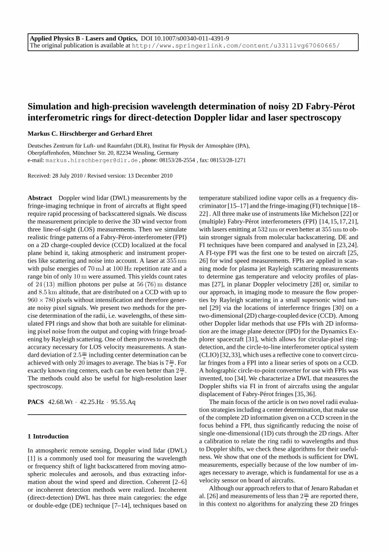
Fig. 1 Measurement principle onboard an aircraft (here DLR Fal-con): see Sec. 2 for details.

in a comprehensible way have been reported yet in combi-nation with results that show the connection of the evaluatedring radii to the Doppler shift. Furthermore we use a rangebin of only 10m (instead of30m in [26]) and no intensifi-cation on the CCD, but still we reach a standard deviation ofless than2m

s by averaging just20 images at8.5 km altitudewith the corresponding environmental conditions. A multi-tude of methods for 2D ring radii calculation of FPI fringeshave been reported in literature, e.g. [37–40], some of themalso including a center evaluation (e.g. [38,40]). While thesemethods are mainly suited for low noise rings in laboratoryexperiments, our approach is also suited for situations withvery noisy rings and the necessity for subpixel accuracy.

The paper is organized as follows: after a description ofthe measurement geometry and a general device setup, wesimulate realistic 2D fringe patterns including atmosphericeffects and noise. Finally we calculate the ring radii (i.e.thewavelengths) of these images and assess the results.

2 Goals and measurement geometry

The goal is a fast and simple instrument for measurements on-board aircrafts in real-time to react to flight-safety endanger-ing phenomena like strong gusts and wake vortices at higherflight altitude and in landing approach or at takeoffs in a dis-tance up to100m in front of them [26]. Figures 1 and 2 il-lustrate the geometrical situation for the determination of a3D wind vector. A laser emitter transmits one pulse of single-mode, single-frequency radiation in each so-called line-of-sight (LOS) direction under an azimuth angle0 ≤ θ < 360

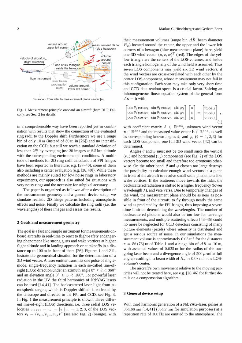
and an elevation angle0 ≤ ϕ < 180. For powerful laserradiation in the UV the third harmonics of Nd:YAG laserscan be used [14,41]. The backscattered laser light from at-mospheric targets, which is Doppler-shifted, is collectedbythe telescope and directed to the FPI and CCD, see Fig. 3.In Fig. 1 the measurement principle is shown: Three differ-ent line-of-sight (LOS) directions, i.e. three radial LOS ve-locities vLOS,i = vi = |vi| , i = 1, 2, 3, of the LOS vec-torsvi = (vx,i, vy,i, vz,i)

T (see also Fig. 2) (orange), with

their measurement volumes (range bin∆R, beam diameterBw) located around the center, the upper and the lower leftcorners of a hexagon (blue measurement plane) here, yieldone 3D wind vector(u, v, w)T (red). The edges of the yel-low triangle are the centers of the LOS-volumes, and insideeach triangle homogeneity of the wind field is assumed. Thusseven LOS components may yield six 3D wind vectors, ifthe wind vectors are cross-correlated with each other by thecenter LOS-component, whose measurement may not fail inthis configuration. Each scan may take only very short timeand CCD data readout speed is a crucial factor. Solving aninhomogeneous linear equation system of the general formAx = b with

cos θ1 cosϕ1 sin θ1 cosϕ1 sinϕ1



uvw

=

vLOS,1

vLOS,2

vLOS,3

,

(1)with coefficient matrixA ∈ R

3×3, unknown wind vectorx ∈ R

3×1 and the measured value vectorb ∈ R3×1, as well

as corresponding known anglesθi andϕi (i = 1, 2, 3) foreach LOS component, one full 3D wind vector [42] can bedetermined.

Anglesθ andϕ must not be too small since the vertical(vx) and horizontal (vy) components (see Fig. 2) of the LOSvectors become too small and therefore too erroneous other-wise. On the other hand,θ andϕ chosen too large destroysthe possibility to calculate enough wind vectors in a planein front of the aircraft to resolve small-scale phenomena likewake vortices. If the scatterers move towards the lidar, thebackscattered radiation is shifted to a higher frequency (lowerwavelengthλ), and vice versa. Due to temporally changes ofthe wind, the measurement plane should be as near as pos-sible in front of the aircraft, to fly through nearly the samewind as predicted by the FPI fringes, thus imposing a severetime limit on determining the wavelengths. The number ofbackscattered photons would also be too low for far-rangemeasurements, and multiple scattering effects [43–45] couldno more be neglected for CCD detectors consisting of manypicture elements (pixels) where intensity is distributed andget a serious source of noise. In our simulations the mea-surement volume is approximately0.05m3 for the distancesr = 56 (76)m of Table 1 and a range bin of∆R = 10m,with assumed values of0.025m for the radius of the out-going laser beam and a divergence angle of500µrad at fullangle, resulting in a beam width ofBw ≈ 0.08m in the LOS-volume’s center.

The aircraft’s own movement relative to the moving par-ticles will not be treated here, see e.g. [26,46] for furtherde-tails on a compensation algorithm.

3 General device setup

With third harmonic generation of a Nd:YAG-laser, pulses at354.88 nm [14,41] (354.7 nm for simulation purposes) at arepetition rate of100Hz are emitted to the atmosphere. The

Simulation and high-precision wavelength determination of noisy 2D Fabry-Perot interferometric rings 3

Fig. 2 Line-of-sight-velocity vectorv (red) and its x-, y-, z-components (green) at a ranger for an azimuth angleθ and an ele-vation angleϕ, and resulting absolute valuevLOS in a constant windfield (u, v, w)T (blue). Two realizations of (θ, ϕ) with vLOS are vi-sualized here.

beams are directed to the variable LOS-directions in depen-dence on time. Some of the pulses are weakened and usedas direct reference signals for frequency stabilization and forDoppler-shift calculations together with the backscattered lightfrom the atmosphere. A wavemeter is required as well for sta-bilizing the seed laser wavelength to stay within the free spec-tral range (FSR) of the FPI (i.e. the same interference order)for unique wavelength assignment (accuracy of±0.002 nmor better required). The receiving telescope collects the backscat-tered photons as well as background radiation of the solarspectrum. After a field stop a fast switch or chopper betweenreference laser signal and backscattered signal is implementedinto the optical paths, that is switched according to the timebetween two consecutive pulses, and whether the signal isused for referencing or for atmospheric backscattering, whichdelays the signal approximately two times the measurementdistance. A schematical setup of the FI-receiver includingonly the most essential parts is shown in Fig. 3. Behind a firstcollecting lens a narrow-band filter blocks most of the broadsolar radiation, allowing only the necessary wavelengths topropagate to an air-spaced Fabry-Perot-etalon. Anotherlenscollects the waves behind the FPI and focuses them to theCCD in the lens focus. This CCD is triggered by the pulseemission time and is activated and paused according to thedesired measurement range. Between the backscatter signals,sometimes one pulse is used as reference signal, which thenmeans a different gating time for the CCD. Finally the noisybackscattered images or the strong reference images are readout very quickly. Algorithms finally calculate the differencein the ring radii of a reference and a backscattered image, andthus the Doppler shift (extracting the true air speed is neces-sary in reality) in one LOS-direction each time.

sun filter

laser-light forreference

lens 1

focusing lens 2

solid- or air-gap-etalonwith two plane-parallelplates at fixed distance

CCD plane

focal length f

plate distance d

refractive index nFPI

interference

multiplereflections

inside plates

backscatteredlight from

atmosphere

chopper orswitch

Fig. 3 Schematical setup of the FI-receiver in this study.

Table 1 Single scattering lidar equation parameters for a transmit-ted pulse energy ofEL = 70mJ and pulse lengthτp = 10 ns at aflight height of8.5 km.

n photons received at CCD 1.3× 107 / 2.4× 107

λL center pulse wavelength 354.7 nmr range 76m / 56mβ(λL, h) backscatter coefficient 3.104 × 10−6 m−1 sr−1

Ar area of the telescope 0.13m2

k instrument constant 0.15α(λL, h) extinction coefficient 2.70× 10−5 m−1

∆R range of atmo. volume 10m

4 Fabry-Perot ring generation including atmosphericeffects and noise

For simulation and visualization of the Fabry-Perot-generatedfringes on the CCD (see Fig. 3), a number of important prop-erties have to be taken into account, see Table 1. These will bediscussed in detail in the following subsections and includedin the FPI ring creation process for an aircraft flight heightof8.5 km. A different approach to generate these FPI rings byray tracing simulations [47] making use of wave propertieswill be described in a forthcoming publication.

4.1 Atmospheric properties

Multiple studies with lidars on the elastic backscatteringandextinction properties for varying heights and regions havebeen carried out [49–52]. A reference model for the atmo-sphere [51,52] from airborne backscatter measurements atspecific wavelengths is applied to estimate the backscatterand extinction coefficients at355 nm.

Rayleigh (molecular) scattering is split into a non-shiftedcenter part, called the Cabannes line, and shifted sidebandsdue to (pure) rotational Raman scattering [53–58]. In thisstudy we use the Gaussian approximation (low density of par-ticles) of the Cabannes line for simplicity.

For our simulations the molecular backscatter coefficientβmol is derived from the Rayleigh backscatter cross sectionper air molecule, which was measured at a (back)scatteringangle ofπ atλ = 0.55µm [59] : dσ/dΩ|π = 5.45×10−32m2 sr−1 .The formula [52]

βmol(h, λ) = 10−7

(

1064 nm

λ

)4.09

exp

(

− h

8000m

)

1

m sr,

(2)


0

0.2

0.4

0.6

0.8

1

-3.0⋅10-10-1.5⋅10-10 0 1.5⋅10-103.0⋅10-10norm

aliz

ed in

tens

ity [a

.u.]

position [a.u.]

(a)

0

0.2

0.4

0.6

0.8

1

-1.0⋅10-12-5.0⋅10-13 0 5.0⋅10-131.0⋅10-12norm

aliz

ed in

tens

ity [a

.u.]

position [a.u.]

(b)

0

0.2

0.4

0.6

0.8

1

-3⋅10-10 0 3⋅10-10norm

aliz

ed in

tens

ity [a

.u.]

position [a.u.]

(c)

0

0.2

0.4

0.6

0.8

1

0 1⋅10-10 2⋅10-10 3⋅10-10norm

aliz

ed in

tens

ity [a

.u.]

position [a.u.]

(d)

0

0.2

0.4

0.6

0.8

1

0 1⋅10-10 2⋅10-10 3⋅10-10norm

aliz

ed in

tens

ity [a

.u.]

position [a.u.]

(e)

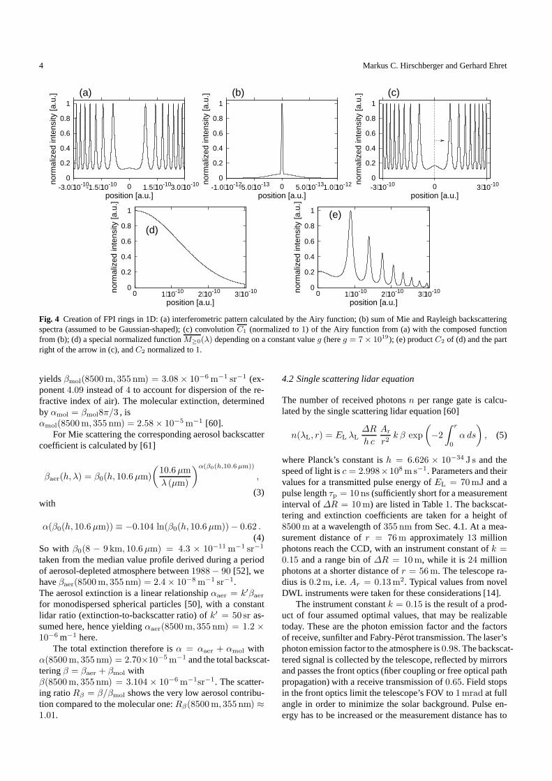
Fig. 4 Creation of FPI rings in 1D: (a) interferometric pattern calculated by the Airy function; (b) sum of Mie and Rayleigh backscatteringspectra (assumed to be Gaussian-shaped); (c) convolutionC1 (normalized to1) of the Airy function from (a) with the composed functionfrom (b); (d) a special normalized functionM≥0(λ) depending on a constant valueg (hereg = 7× 1019); (e) productC2 of (d) and the partright of the arrow in (c), andC2 normalized to1.

yieldsβmol(8500m, 355 nm) = 3.08× 10−6m−1 sr−1 (ex-ponent4.09 instead of4 to account for dispersion of the re-fractive index of air). The molecular extinction, determinedbyαmol = βmol8π/3 , isαmol(8500m, 355 nm) = 2.58× 10−5m−1 [60].

For Mie scattering the corresponding aerosol backscattercoefficient is calculated by [61]

βaer(h, λ) = β0(h, 10.6µm)

(

10.6µm

λ (µm)

)α(β0(h,10.6µm))

,

(3)with

α(β0(h, 10.6µm)) ≡ −0.104 ln(β0(h, 10.6µm))− 0.62 .(4)

So with β0(8 − 9 km, 10.6µm) = 4.3 × 10−11m−1 sr−1

taken from the median value profile derived during a periodof aerosol-depleted atmosphere between1988− 90 [52], wehaveβaer(8500m, 355 nm) = 2.4× 10−8m−1 sr−1.The aerosol extinction is a linear relationshipαaer = k′βaer

for monodispersed spherical particles [50], with a constantlidar ratio (extinction-to-backscatter ratio) ofk′ = 50 sr as-sumed here, hence yieldingαaer(8500m, 355 nm) = 1.2 ×10−6 m−1 here.

The total extinction therefore isα = αaer + αmol withα(8500m, 355 nm) = 2.70×10−5m−1 and the total backscat-teringβ = βaer + βmol withβ(8500m, 355 nm) = 3.104 × 10−6m−1sr−1. The scatter-ing ratioRβ = β/βmol shows the very low aerosol contribu-tion compared to the molecular one:Rβ(8500m, 355 nm) ≈1.01.

4.2 Single scattering lidar equation

The number of received photonsn per range gate is calcu-lated by the single scattering lidar equation [60]

n(λL, r) = EL λL∆R

h c

Ar

r2k β exp

(

−2

∫ r

0

α ds

)

, (5)

where Planck’s constant ish = 6.626 × 10−34 J s and thespeed of light isc = 2.998×108ms−1. Parameters and theirvalues for a transmitted pulse energy ofEL = 70mJ and apulse lengthτp = 10 ns (sufficiently short for a measurementinterval of∆R = 10m) are listed in Table1. The backscat-tering and extinction coefficients are taken for a height of8500m at a wavelength of355 nm from Sec. 4.1. At a mea-surement distance ofr = 76m approximately13 millionphotons reach the CCD, with an instrument constant ofk =0.15 and a range bin of∆R = 10m, while it is 24 millionphotons at a shorter distance ofr = 56m. The telescope ra-dius is0.2m, i.e.Ar = 0.13m2. Typical values from novelDWL instruments were taken for these considerations [14].

The instrument constantk = 0.15 is the result of a prod-uct of four assumed optimal values, that may be realizabletoday. These are the photon emission factor and the factorsof receive, sunfilter and Fabry-Perot transmission. The laser’sphoton emission factor to the atmosphere is0.98. The backscat-tered signal is collected by the telescope, reflected by mirrorsand passes the front optics (fiber coupling or free optical pathpropagation) with a receive transmission of0.65. Field stopsin the front optics limit the telescope’s FOV to1mrad at fullangle in order to minimize the solar background. Pulse en-ergy has to be increased or the measurement distance has to


be reduced if this factor is lower than0.65 in reality. At aFWHM of 0.5 nm the sunfilter transmits a factor of0.95. Fora low reflectivity of0.70 of the FPI plates the losses insidethe etalon are relatively low, not considering absorptionof theplates. Depending on the width of the fringes, the correctedtransmission factor of the etalon onto the CCD, calculatedby integrating the intensity columns of patterns like the oneshown in Fig. 4(e) and dividing them by intensity columnsof maximum value1, may slightly vary around0.25. So0.25was chosen as a mean value.

4.3 Mie and Rayleigh scattering

Simulations were performed with Gaussian models of Mieand Rayleigh scattering. Mie and Rayleigh scattering func-tions in our case are needed for a convolution to create ringsof different widths depending on temperature and pressureor heights according to US Standard atmosphere [62]. Thecalculations will be valid for all kinds of FPI rings with sym-metrically shaped peaks over a background.

The first step is carried out one-dimensional. The Rayleighscattering line shape is governed by broadening which resultsin the following Gaussian line profile function [50,60] cen-tered aroundλL:

IR(λ) =1

√

2πσ 2R

exp

(

−0.5(λ− λL)

2

σ 2R

)

, (6)

whereσR denotes the standard deviation of the Rayleigh spec-trum given by

σR(mair) =2λL

c

√

kBTNA

mair, (7)

wheremair = 2.9 × 10−2kg/mol is the mean molecular airmass,λL is the laser wavelength,kB = 1.38×10−23J/K theBoltzmann constant,T (8500m) = 232.9K the temperature,c the speed of light, andNA = 6.023× 1023mol−1 the Avo-gadro constant.

The laser beam intensity is assumed to have a Gaussianshaped spectral distribution [63]:

IL(λ) = πτ 2p exp(−0.5(∆ω)2τ 2

p ) , (8)

with pulse lengthτp = 10 ns and frequency interval∆ω =2πc(λ − λL)/λ

2L . The step resolutionλ is used for model-

ing. The full width at half maximum of (8) is∆λLFWHM=

2|λI,max − λLFWHM|, with theλ-value of peak intensity (the

center)λI,max and the distanceλLFWHMto it. The aerosol

(Mie) scattering spectrumIM(λ), governed by the laser pro-file, looks like that of (6), replacing onlyIR by IM andσR byσM, with

σM =∆λLFWHM√

8 · ln 2, (9)

where∆λLFWHMis the full width at half maximum (FWHM)

of the Gaussian laser spectrum mentioned afore. The Miepeak is added to the broadband Rayleigh part, see Fig. 4 (b).The shape of this pattern is important, hence the diagramswith arbitrary units illustrate the principle.

0

0.2

0.4

0.6

0.8

1

0 1⋅10-10 2⋅10-10 3⋅10-10

norm

aliz

ed in

tens

ity [a

.u.]

position [a.u.]

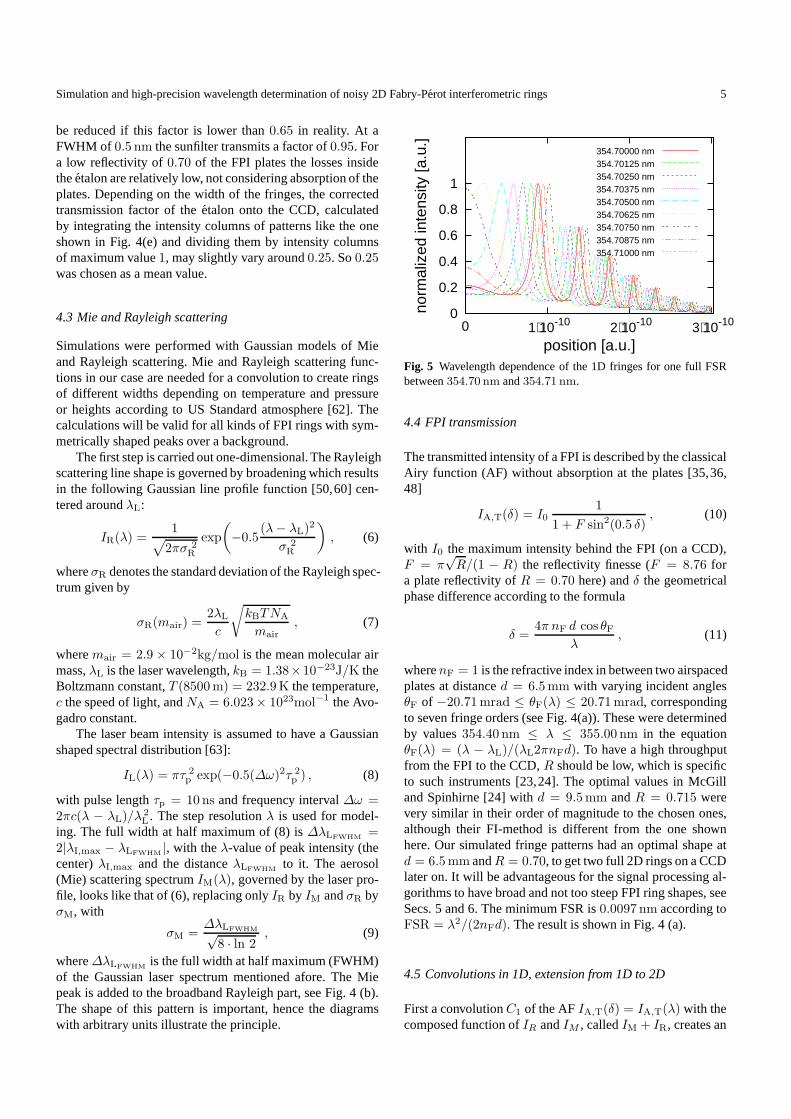
354.70000 nm354.70125 nm354.70250 nm354.70375 nm354.70500 nm354.70625 nm354.70750 nm354.70875 nm354.71000 nm

Fig. 5 Wavelength dependence of the 1D fringes for one full FSRbetween354.70 nm and354.71 nm.

4.4 FPI transmission

The transmitted intensity of a FPI is described by the classicalAiry function (AF) without absorption at the plates [35,36,48]

IA,T(δ) = I01

1 + F sin2(0.5 δ), (10)

with I0 the maximum intensity behind the FPI (on a CCD),F = π

√R/(1 − R) the reflectivity finesse (F = 8.76 for

a plate reflectivity ofR = 0.70 here) andδ the geometricalphase difference according to the formula

δ =4π nF d cos θF

λ, (11)

wherenF = 1 is the refractive index in between two airspacedplates at distanced = 6.5mm with varying incident anglesθF of −20.71mrad ≤ θF(λ) ≤ 20.71mrad, correspondingto seven fringe orders (see Fig. 4(a)). These were determinedby values354.40 nm ≤ λ ≤ 355.00 nm in the equationθF(λ) = (λ − λL)/(λL2πnFd). To have a high throughputfrom the FPI to the CCD,R should be low, which is specificto such instruments [23,24]. The optimal values in McGilland Spinhirne [24] withd = 9.5mm andR = 0.715 werevery similar in their order of magnitude to the chosen ones,although their FI-method is different from the one shownhere. Our simulated fringe patterns had an optimal shape atd = 6.5mm andR = 0.70, to get two full 2D rings on a CCDlater on. It will be advantageous for the signal processing al-gorithms to have broad and not too steep FPI ring shapes, seeSecs. 5 and 6. The minimum FSR is0.0097 nm according toFSR = λ2/(2nFd). The result is shown in Fig. 4 (a).

4.5 Convolutions in 1D, extension from 1D to 2D

First a convolutionC1 of the AFIA,T(δ) = IA,T(λ) with thecomposed function ofIR andIM , calledIM + IR, creates an


underground below the AF (Fig. 4 (c)) and may broaden thefinal fringes via

C1(λ) = (IA,T ∗ (IM + IR))(λ)

=

∫

R

IA,T(x) (IM + IR)(λ− x) dx ,(12)

where∗ denotes the convolution operator. The segment widthhas to be equal forIA,T(λ) andIM+ IR. Then the maximumof C1 is determined and set to the value1; the whole graphis stretched or jolted, see Fig. 4 (c), resulting in the functionC1.

A decay of the intensity to the points more distant fromthe ring center is observed in reality, see [26,33,39,40,48].This is here accomplished by multiplication ofC1, takingonly the points right of the ring center (arrow in Fig. 4 (c)),with the branch to the right of the maximum of a special func-tion

M(λ) =

√

g

2πexp

(

−g λ2

2

)

, (13)

with a constantg = 7× 1019 (appropriate for the dimensionsof the position-axis), that was picked here due to its decayproperty.M(λ) has no physical meaning and is used to modeldifferent steepnesses of peak decays by varyingg (Fig. 4 (d)).Only λ-values greater zero are taken and the maximum ofMis normalized to1, resulting in a functionM≥0(λ). The prod-uct isC2(λ) = C1(λ) · M≥0(λ), which is normalized to arotational-symmetric functionC2(λ) around0 (Fig. 4 (e)).

Fig. 5 shows the wavelength-dependence of fringe pat-terns like the one shown in Fig. 4 (e) over one full FSR. Forthe wavelength-determination algorithms it will be advanta-geous to have the first peak away from the center as far aspossible, to have more pixels to average later on. A wave-length ofλ = 354.70000 nm (i.e. the center wavelength inour simulations) is therefore best suited in this case, whileλ = 354.70625 nm with the first peak at the center wouldbe a bad choice. The useful part of the FSR for the measure-ments should therefore be limited to±0.002 nm around thecenter wavelength.

From that (Figs. 4(e) and 5) a 2D, rotational-symmetricpattern of non-equidistant rings can be created. Dependingon the width of the convolving functionIM + IR a quadraticimage of equal number of points with equidistant segmentwidths on thex- andy-axes arises, each tuple(x, y) ∈ R

2 be-ing a pixel. The number of points on each axis after convolu-tions in 1D usually was between506 and541. In 2D the num-ber of points on each axis is doubled by symmetry around0.CCD imagers normally are non-quadratic, so on each axis anumber of points are dropped (see Figs. 6 (a), (b)), and in-stead of1010× 1010 pixels any lower dimension can be cho-sen; in our case it is961 × 781 pixels (see Figs. 6 (c), (d)),since odd numbers yield a unique center pixel at(0, 0) andfor the algorithms a pixel number as high as possible shouldbe aimed at.

4.6 Noise modeling by random number generation

A PCO dicam pro intensified-CCD (ICCD) camera [64] andits specifications may serve as a sample for a suitable imag-ing device. Most of the parameters for the simulations arechosen in the order of magnitude of this camera’s specifica-tions. A model of this series was used for DWL measure-ments in an aircraft [25]. However, a CCD’s noise proper-ties were modeled here, which means an excess noise factor(ENF) ofENFCCD ≈ 1 (i.e. gain factor of 1, no excess noise)[65], while it is ENFICCD ≈ 2 for an ICCD with gain fac-tors of 100 and higher [65]. Intensification is excluded forsimplicity and to simulate a worst-case scenario in this study.Despite the fact that the ICCD shows a larger ENF, this de-vice usually provides a greater signal-to-noise ratio (SNR)than a CCD, as shown by Carranza et al. [66] for a spectralrange around400 nm. The shortest shutter of the ICCD cam-era is as low as3 ns, thus realization of intervals of67 ns(range gate∆R = 10m) is possible. One hundred pulses persecond means100 CCD images (see Sec. 3) and in this wayabout10ms time to readout the data of one image, before thisstep is repeated. The laser is linked to the CCD to trigger theCCD shutter with the moment of pulse emission.

Three main sources of noise distort the optimal shape ofthe rings shown in Figs. 6 (a) and (b). For the reference signalspeckle noise is relevant, at insignificantly low photon noise.The backscattered signal comprises neglectable speckle noise,while photon noise is dominating. The CCD’s readout noiseoccurs for both signal types.

Dark current noise can be ignored owing to the short gatetime of67 ns and the narrow-band filter in the receiver. Usualdark currents are lower than100 electrons per second for eachpixel, so it should be maximum0.67 × 10−6 electrons perpixel in 67 ns in our case. Solar noise can also be excludedfrom modeling, see Sec. 4.7.

Artificial creation of noise implies using a modern, non-standard, fast random number generator (RNG) like Ran ofNumerical Recipes [67] for uniform deviates with sufficientlylong period to create variable values without repetition. Theseed values to start the RNG must be chosen differently forevery picture.

CCDs are arrays of light-sensitive photodiodes that gen-erate and store electrons from photons with a certain quantumefficiencyη (η ≈ 0.21 for dicam CCD at355 nm) [68]. Wedefine the number of signal (photo) electrons (e−) generatedby a numbern of backscattered (calculated by (5)) or directphotons by

nsg = η n . (14)

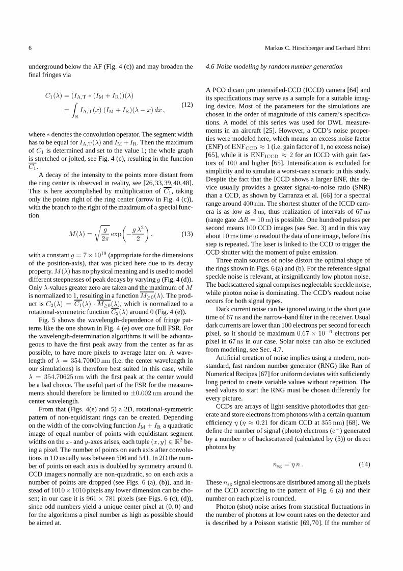
Thesensg signal electrons are distributed among all the pixelsof the CCD according to the pattern of Fig. 6 (a) and theirnumber on each pixel is rounded.

Photon (shot) noise arises from statistical fluctuations inthe number of photons at low count rates on the detector andis described by a Poisson statistic [69,70]. If the number of


Fig. 6 Creation of FPI ringsin 2D on a CCD (contin-ued from Fig. 4): (a) 2D,rotational-symmetric patternof non-equidistant rings atλ = 354.7000 nm after non-quadratic area reduction from asquare to a rectangular shapedCCD image; (b) the same as (a)for λ = 354.7075 nm; (c) pat-tern atλ = 354.7000 nm afterrestructuring of the positionsin (a) to pixel numbers, anddistribution of photoelectronsonto the pixels of the CCDimage; (d) the same as (c) fora broad ring structure due toconvolution.

signal electrons on a single pixel with indexi is nsg,i, then

nsg =1

m · n

m·n∑

i=1

nsg,i (15)

denotes the average signal electrons on each pixel (the meanand variance of a Poisson deviate), wherem andn are thex-andy-axes dimensions (e.g.m = 961 andn = 781 pixels inFig. 6), respectively. In order to simulate the number ofe−,the Ran-RNG [67] was used to genereate Poisson-distributedrandom numbers by the so-called rejection-method [67]. Theprobability distribution is

PPoi,nsg(Xsg,i = nsg,i) =

nsgnsg,i

(nsg,i)!exp(−nsg) , (16)

which denotes the probability, that the random numbers (vari-ables)Xsg,i will take the values (realizations)nsg,i [70].

Gamma-distributed random numbers serve for character-ization of speckle noise, with parameterssi for the number ofspeckle grains averaged on thei-th pixel which can be mea-sured for each pixel; we took an average value ofs = 10.0for all the si, since similar values were measured [70]. Theprobability distribution is

PΓ (Xsg,i = nsg,i) =1

Γ (si)

(

sinsg

)si

nsi−1sg,i exp

(

−sinsg,i

nsg

)

,

(17)with a mean ofnsg, a variance of(nsg

2)/si, and a Gamma-functionΓ (·) that is commonly defined.

The CCD’s readout noise obeys a Gaussian-distribution,thus normal deviates created by the ratio-of-uniforms method

[67] are taken, with a probability distribution

PN (µ,σ2) (Xsg,i = nsg,i) =1√2πσ2

exp

(

− (µ− nsg,i)2

2σ2

)

,

(18)with the meanµ = 0 and the varianceσ2 (σ may vary de-pending on the type of CCD; hereσ = 5.0 was chosen, simi-lar to a measured value for a CCD [70]).

For simulations of backscatter signals (as shown in Fig. 6),the final number of charge carriers on a pixeli is

nC,i = RNPoi,i +RNN ,i , (19)

whereRNPoi,i andRNN ,i are the random numbers includ-ing photon and readout noise, respectively, that were createdusing the probability distributions specified in (16) and (18).For reference signals or for calibration we have

nC,i = RNΓ,i +RNN ,i , (20)

whereRNΓ,i are the random numbers including speckle noiserelated to (17). Thus uncorrelated noise sources (especiallyphoton and speckle noise [71]) can be assumed, i.e. the ran-dom numbers are independent and can be summed. Negativenumbers ofnC,i, which may occur due to the normal devi-ates, are set to zero (numbers ofe− lower 0 are impossible).Results of differently broad rings for backscatter signalsatr = 56m (24 million photons) due to modeling, includingnoise, are shown in Figs. 6 (c) and (d).

4.7 Solar background

If the sky is clear, i.e. at lack of aerosols, the lidar will detectsolar radiance (direct and scattered by molecules) besidesthe


0

100

200

300

400

500

600

700

300 400 500 600 700 800

radi

ance

[mW

/(m

2 nm

sr)

]

solar wavelength [nm]354.7

100 150 200 250 300 350 400 450

350 360354.7

Fig. 7 Received solar spectrum from290− 800 nm.

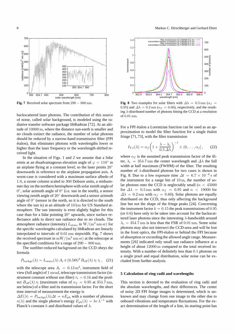
backscattered laser photons. The contribution of this sourceof noise, called solar background, is modeled using the ra-diative transfer software package libRadtran [72]. At an alti-tude of10000m, where the distance sun-earth is smaller andno clouds extinct the radiance, the number of solar photonsshould be reduced by a narrow-band transmissive filter (FPIetalon), that eliminates photons with wavelengths lower orhigher than the laser frequency or the wavelength-shifted re-ceived light.

In the situation of Figs. 1 and 2 we assume that a lidaremits at an disadvantageous elevation angle ofϕ = 110 inan airplane flying at a constant level; so the laser points20

downwards in reference to the airplane propagation axis. Aworst-case is considered with a maximum surface albedo of1.0, a ozone column scaled to300 Dobson units, a midsum-mer day on the northern hemisphere with solar zenith angle of0, solar azimuth angle of0 (i.e. sun in the south), a sensorviewing zenith angle of20 downwards and a sensor azimuthangle of0 (sensor in the north, so it is directed to the southwhere the sun is) at an altitude of10 km for US Standard at-mosphere. The sun intensity is even slightly higher for thiscase than for a lidar pointing20 upwards, since surface re-flectance adds to direct sun radiance due to no clouds. Theatmosphere radiance (intensity)Latmo in W/(m2 nm sr) forthe specific wavelengths calculated by libRadtran are linearlyinterpolated to intervals of0.01 nm stepwidth. Fig. 7 showsthe received spectrum inmW/(m2 nm sr) at the telescope atthe specified conditions for a range of290− 800 nm.

The sunfilter-reduced background on the CCD obeys theformula

Pbackgr(λ) = Latmo(λ)Ar π (0.5Θ)2 Beff(λ) τf τt , (21)

with the telescope areaAr = 0.13m2, instrument field ofview (full angle) of1mrad, telescope transmission factor (in-strument constant without sun filter)τt = 0.16 and the prod-uct Beff(λ) τf (maximum value ofαf = 0.95 at 354.7 nm,see below) of a filter and its transmission factor. For the shorttime interval of measurement the energy is∆E(λ) = Pbackgr(λ)∆t = nEph with a number of photonsn(λ) and the single photon’s energyEph(λ) = hc λ−1 withPlanck’s constanth and distributed values ofλ.

0

0.2

0.4

0.6

0.8

1

1.2

1.4

352.9 353.5 354.1 354.7 355.3 355.9 356.5 0

100

200

300

400

500

600

700

tran

smis

sion

num

ber

of p

hoto

ns

wavelength [nm]

filter transmission for FWHM=0.5 nmtransmitted number of photons for FWHM=0.5 nm

filter transmission for FWHM=0.2 nmtransmitted number of photons for FWHM=0.2 nm

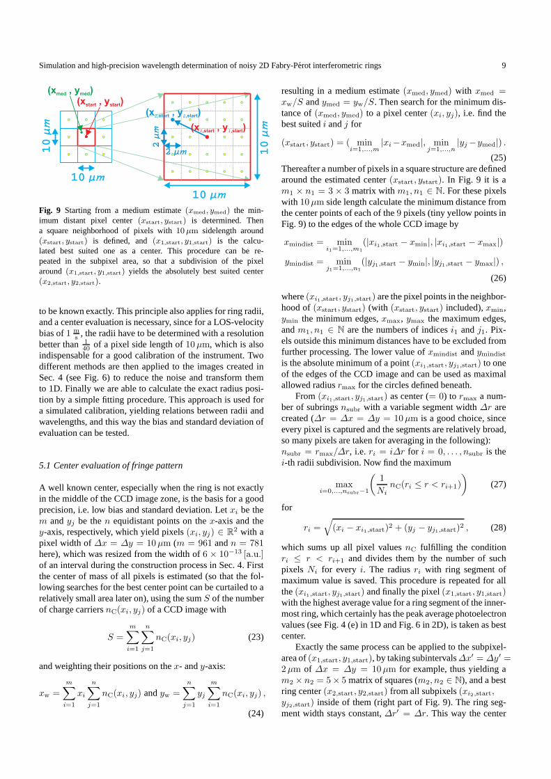
Fig. 8 Two examples for solar filters with∆λ = 0.5 nm (αf =0.95) and∆λ = 0.2 nm (αf = 0.60), respectively, and the result-ing λ-distributed number of photons hitting the CCD at a resolutionof 0.01 nm.

For a FPI etalon a Lorentzian function can be used as an ap-proximation to model the filter function for a single etalonfringe [71,73], with the filter transmission

IT,f(λ) = αf

(

1 +λ− λc

0.5∆λ

)−1

∈ (0, . . . , αf ] , (22)

whereαf is the assumed peak transmission factor of the fil-ter, λc = 354.7 nm the center wavelength and∆λ the fullwidth at half maximum (FWHM) of the filter. The resultingnumber ofλ-distributed photons for two cases is shown inFig. 8. Due to a low exposure time∆t = 6.7 × 10−8 s ofthe instrument for a range bin of10m, the number of so-lar photons onto the CCD is neglectably small (n < 45000for ∆λ = 0.5 nm with αf = 0.95 and n < 19000 for∆λ = 0.2 nm with αf = 0.60). Solar photons are equallydistributed on the CCD, thus only affecting the backgroundline but not the shape of the fringe peaks [24]. Concerningthe instrument factork = 0.15 the peak transmissions of0.95(or 0.6) have only to be taken into account for the backscat-tered laser photons since the interestingλ-bandwidth aroundλc = 354.7 nm is less than the FSR of0.01 nm. Some solarphotons may also not intersect the CCD-area and will be lostin the front optics, the FPI-etalon or behind the FPI becauseof absorption or exceeding the allowed angle range. Measure-ments [26] indicated only small sun radiance influence at aheight of about12000m compared to the total received in-tensity. With a number of definitely less than0.1 photons ona single pixel and equal distribution, solar noise can be ex-cluded from further analysis.

5 Calculation of ring radii and wavelengths

This section is devoted to the evaluation of ring radii andthe absolute wavelengths, and their differences. The centerof noisy 2D FPI fringe images is determined, which is un-known and may change from one image to the other due toonboard vibrations and temperature fluctuations. For the ex-act determination of the length of a line, its starting pointhas


10 mm

10

mm

10 mm

10

mm

2 mm2

mm (x , y )

1 1,start ,start

(x , y )2 2,start ,start

(x , y )med med

(x , y )start start

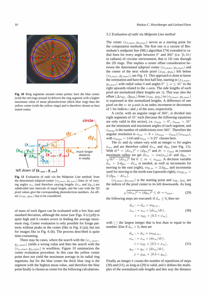
Fig. 9 Starting from a medium estimate(xmed, ymed) the min-imum distant pixel center(xstart, ystart) is determined. Thena square neighborhood of pixels with10µm sidelength around(xstart, ystart) is defined, and(x1,start, y1,start) is the calcu-lated best suited one as a center. This procedure can be re-peated in the subpixel area, so that a subdivision of the pixelaround(x1,start, y1,start) yields the absolutely best suited center(x2,start, y2,start).

to be known exactly. This principle also applies for ring radii,and a center evaluation is necessary, since for a LOS-velocitybias of1 m

s , the radii have to be determined with a resolutionbetter than1

40 of a pixel side length of10µm, which is alsoindispensable for a good calibration of the instrument. Twodifferent methods are then applied to the images created inSec. 4 (see Fig. 6) to reduce the noise and transform themto 1D. Finally we are able to calculate the exact radius posi-tion by a simple fitting procedure. This approach is used fora simulated calibration, yielding relations between radiiandwavelengths, and this way the bias and standard deviation ofevaluation can be tested.

5.1 Center evaluation of fringe pattern

A well known center, especially when the ring is not exactlyin the middle of the CCD image zone, is the basis for a goodprecision, i.e. low bias and standard deviation. Letxi be them andyj be then equidistant points on thex-axis and they-axis, respectively, which yield pixels(xi, yj) ∈ R

2 with apixel width of∆x = ∆y = 10µm (m = 961 andn = 781here), which was resized from the width of6 × 10−13 [a.u.]of an interval during the construction process in Sec. 4. Firstthe center of mass of all pixels is estimated (so that the fol-lowing searches for the best center point can be curtailed toarelatively small area later on), using the sumS of the numberof charge carriersnC(xi, yj) of a CCD image with

S =

m∑

i=1

n∑

j=1

nC(xi, yj) (23)

and weighting their positions on thex- andy-axis:

xw =

m∑

i=1

xi

n∑

j=1

nC(xi, yj) andyw =

n∑

j=1

yj

m∑

i=1

nC(xi, yj) ,

(24)

resulting in a medium estimate(xmed, ymed) with xmed =xw/S andymed = yw/S. Then search for the minimum dis-tance of(xmed, ymed) to a pixel center(xi, yj), i.e. find thebest suitedi andj for

(xstart, ystart) = ( mini=1,...,m

|xi−xmed|, minj=1,...,n

|yj−ymed|) .(25)

Thereafter a number of pixels in a square structure are definedaround the estimated center(xstart, ystart). In Fig. 9 it is am1 × n1 = 3 × 3 matrix withm1, n1 ∈ N. For these pixelswith 10µm side length calculate the minimum distance fromthe center points of each of the9 pixels (tiny yellow points inFig. 9) to the edges of the whole CCD image by

xmindist = mini1=1,...,m1

(|xi1,start − xmin|, |xi1,start − xmax|)

ymindist = minj1=1,...,n1

(|yj1,start − ymin|, |yj1,start − ymax|) ,(26)

where(xi1,start, yj1,start) are the pixel points in the neighbor-hood of(xstart, ystart) (with (xstart, ystart) included),xmin,ymin the minimum edges,xmax, ymax the maximum edges,andm1, n1 ∈ N are the numbers of indicesi1 andj1. Pix-els outside this minimum distances have to be excluded fromfurther processing. The lower value ofxmindist andymindist

is the absolute minimum of a point(xi1,start, yj1,start) to oneof the edges of the CCD image and can be used as maximalallowed radiusrmax for the circles defined beneath.

From(xi1,start, yj1,start) as center (= 0) to rmax a num-ber of subringsnsubr with a variable segment width∆r arecreated (∆r = ∆x = ∆y = 10µm is a good choice, sinceevery pixel is captured and the segments are relatively broad,so many pixels are taken for averaging in the following):nsubr = rmax/∆r, i.e. ri = i∆r for i = 0, . . . , nsubr is thei-th radii subdivision. Now find the maximum

maxi=0,...,nsubr−1

(

1

Ni

nC(ri ≤ r < ri+1)

)

(27)

for

ri =√

(xi − xi1,start)2 + (yj − yj1,start)

2 , (28)

which sums up all pixel valuesnC fulfilling the conditionri ≤ r < ri+1 and divides them by the number of suchpixels Ni for every i. The radiusri with ring segment ofmaximum value is saved. This procedure is repeated for allthe(xi1,start, yj1,start) and finally the pixel(x1,start, y1,start)with the highest average value for a ring segment of the inner-most ring, which certainly has the peak average photoelectronvalues (see Fig. 4 (e) in 1D and Fig. 6 in 2D), is taken as bestcenter.

Exactly the same process can be applied to the subpixel-area of(x1,start, y1,start), by taking subintervals∆x′ = ∆y′ =2µm of ∆x = ∆y = 10µm for example, thus yielding am2 × n2 = 5× 5 matrix of squares (m2, n2 ∈ N), and a bestring center(x2,start, y2,start) from all subpixels(xi2,start,yj2,start) inside of them (right part of Fig. 9). The ring seg-ment width stays constant,∆r′ = ∆r. This way the center


Fig. 10 Ring segments around center points: here the blue center(with the red rings around it) delivers the ring segment witha highermaximum value of mean photoelectrons (thick blue ring) thantheyellow center (with the yellow rings) and is therefore chosen as bestsuited center.

2 mm

2 m

m

(x , y )1 1,start ,startDxML

DyML(x , y )ML ML

left down of (x , y )2 2,start ,start

(x , y )2 2,start ,start

much longerdistancein reality

dym

dxm

dr

am

circle

Fig. 11 Evaluation of radii via the Midpoint Line method: fromthe determined subpixel-center(x2,start, y2,start) linesdr of vary-ing anglesαm (and therefore varying lengthsdxm anddym) aresubdivided into intervals of equal length, and the cuts withthe 2Dpixel values give the corresponding photoelectron numbers. An off-set(xML, yML) has to be considered.

of mass of each figure can be evaluated with a low bias andstandard deviation, although the noise (see Figs. 6 (c),(d)) isquite high and it creates errors in finding the average maxi-mum ring. Center evaluation is only possible for fringe pat-terns without peaks in the center (like in Fig. 6 (a)), but notfor images like in Fig. 6 (b). The process described is quitetime-consuming.

There may be cases, where the search with the(xi1,start,yj1,start) yields a wrong value and then the search with the(xi2,start, yj2,start) is worthless. Figure 10 summarizes thecenter evaluation procedure. In this case the yellow centerpoint does not yield the maximum average in its radial ringsegments, but for the blue center the thick blue ring is thesegment with the highest mean value, and therefore the bluepoint finally is chosen as center for the following calculations.

5.2 Evaluation of radii via Midpoint Line method

The center(x2,start, y2,start) serves as a starting point forthe computation methods. The first one is a variant of Bre-senham’s midpoint line (ML) algorithm [74] extended to ra-dial lines for every angle between0 and360 (i.e. [0, 2π)in radians) of circular environment, that is 1D cuts throughthe 2D rings. This implies a center offset consideration be-tween the determined subpixel center(x2,start, y2,start) andthe center of the next whole pixel(xML, yML) left below(x2,start, y2,start), see Fig. 11. This approach is done to knowthe orientation and have the first half line, starting in(x2,start,y2,start) with radial value0 and angles0 ≤ α ≤ 45 to theright upwards related to thex-axis. The side lengths of eachpixel are normalized (their lengths are1). This way also theoffset(∆xML, ∆yML) from (xML, yML) to (x2,start, y2,start)is expressed in this normalized lengths. A difference of onepixel on thex- or y-axis is an index increment or decrementof 1 for indicesi andj of the axes, respectively.

A circle, with an angular range of360, is divided intoeight segments of45 each (because the following equationsare only valid in this sector), i.e.αmin = 0, αmax = 45

are the minimum and maximum angles of each segment, andαsteps is the number of subdivisions over360. Therefore theangular resolution isαres = 8 × (αmax − αmin)/(αsteps),with αsteps = 1440 andαres = 0.25 chosen here.

Thedx anddy values vary with an integerm for anglesαm, and are therefore calleddxm and dym (see Fig. 11).With dr2 = (dxm)2 + (dym)2 anddr = rmax as constantmaximum radius we getdxm = cos(αm) dr and dym =√

dr2 − (dxm)2 for 0 ≤ m < αmax. A decision variabledm = 2 dym − dxm is needed, as well as increments formoving to the east (right),inE,m = 2 dym, and incrementsused for moving to the north-east (upwards-right),inNE,m =2 (dym − dxm).

(x2,start, y2,start) is the starting point andiML, jML arethe indices of the pixel center to its left downwards. As longas

√

(dxm)2 + (dym)2 ≤ dr = rmax , (29)

the following steps are executed: ifdm ≤ 0, then set

dm : = dm + inE,m ,

xm : = xm + (dxm/dr) ,

i = iML + ⌊0.5 + xm⌋.(30)

with ⌊·⌋ the largest integer that is less than or equal to thenumber. Else ifdm > 0, then set

dm : = dm + inNE,m ,

xm : = xm + (dxm/dr) ,

i = iML + ⌊0.5 + xm⌋ ,ym : = ym + (dxm/dr) ,

j = jML + ⌊0.5 + ym⌋.

(31)

Finally an integerk counts the number of repetitions of steps(30) and (31), as long as (29) is valid, andk defines the multi-ples of the normalized side lengths and this way the distance


from the center. Note that this solely describes the procedurefor angles0 ≤ αm < 45. The formulas in (30) and (31)and before need only be slightly adapted for the other 7 sec-tors covering45 each. For example,dxm = − cos(αm) dr,or dm = 2 dxm − dym, or ym := ym − (dxm/dr) andj = jML − ⌊0.5 + ym⌋, and so on, are possible changes,that have to be combined due to geometrical and symmetricalconsiderations for all sectors.

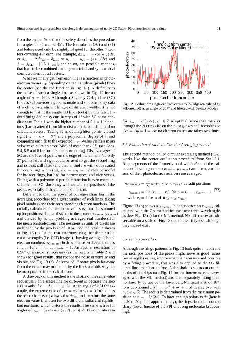
What we finally get from each line is a function of photo-electron valuesnC depending on radius values (pixels) fromthe center (see the red function in Fig. 12). A difficulty isthe noise of such a single line, as shown in Fig. 12 for anangle ofα = 269. Although a Savitzky-Golay filter (SG)[67,75,76] provides a good estimate and smooths noisy dataof such non-equidistant fringes of different widths, it is notenough to just fit the single 1D lines (cuts) by this filter. In-deed fitting360 noisy cuts in steps of1 with SG at the con-ditions of Table 1 with the higher number of2.4 × 107 pho-tons (backscattered from56m distance) delivers big randomcalculation errors. Taking37 smoothing filter points left andright (nL = nR = 37) and a polynomial degree of 4, andcomparing each fit to the expectedvLOS-value yields a meanvelocity calculation error (bias) of more than50m

s (see Secs.5.4, 5.5 and 6 for further details on fitting). DisadvantagesofSG are the loss of points on the edge of the domain (so only37 points left and right could be used to get the second ringand its peak still fitted) and thatnL andnR will not be suitedfor every ring width (e.g.nL = nR = 37 may be usefulfor broader rings, but bad for narrow ones, and vice versa).Fitting with a polynomial periodic function is even more un-suitable than SG, since they will not keep the positions of thepeaks, especially if they are nonequidistant.

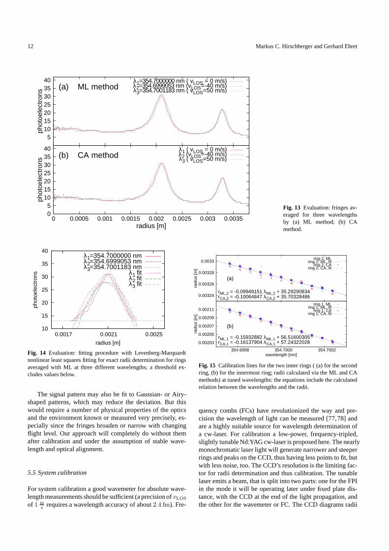
Different to that, the power of our algorithms lies in theaveraging procedure for a great number of such lines, takingpixel numbers and their corresponding electron numbers. Theradially calculated photoelectron valuesnC must be summedup for positions of equal distance to the center(x2,start, y2,start)and divided byαsteps, yielding averaged real numbers forthe mean photoelectrons. The positions in units of pixels aremultiplied by the pixelsize of10µm and the result is shownin Fig. 13 (a) for the two innermost rings for three differ-ent wavelengths (i.e. CCD images), showing averaged photo-electron numbersnC,mean,i in dependence on the radii valuesrmean,i for i = 0, . . . , nsubr − 1. An angular resolution of0.25 of a circle is necessary (as the results in Table 2 willshow) for good results, that reduce the noise drastically andvisible, see Fig. 13 (a). At steps of1 some pixels far awayfrom the center may not be hit by the lines and this way notbe incorporated in the calculations.

A drawback of this method is the choice of the same valuesequentially on a single line for differentk, because the stepsize is only∆x = ∆y = 1 ≥ ∆r. At an angle ofπ/4 for ex-ample, the extreme case of∆r = cos(π/4) = 0.707 < 1 isthe reason for having a low valuedxm, and therefore the sameelectron value is chosen for two different radial and equidis-tant positions, which distorts the results. The same is trueforangles ofαm = (π/4)+k′(π/2) , k′ ∈ Z. The opposite case

0

5

10

15

20

25

30

35

40

0 50 100 150 200 250 300 350 400

phot

oele

ctro

ns

pixel number from center

ring cut from centerSavitzky-Golay filtered

Fig. 12 Evaluation: single cut from center to the edge (calculated byML-method) at an angle of269 and filtered with Savitzky-Golay.

for αm = k′(π/2) , k′ ∈ Z is optimal, since then the cutsthrough the 2D rings lie on thex- or y-axes and according to∆x = ∆y = 1 = ∆r no electron values are taken two times.

5.3 Evaluation of radii via Circular Averaging method

The second method, called circular averaging method (CA),works like the center evaluation procedure from Sec. 5.1.Ring segments of the formerly used width∆r and the cal-culated best ring center(x2,start, y2,start) are taken, and thesum of their photoelectron numbers are averaged:

nC,mean,i =1

Ni

nC(ri ≤ r < ri+1) at radii positions

rmean,i = 0.5 (ri+1 − ri) for i = 0, . . . , nsubr − 1

with ri = i∆r and 0 ≤ r ≤ rmax.

(32)

Figure 13 (b) showsnC,mean,i in dependence onrmean,i cal-culated with the CA method for the same three wavelengthsas does Fig. 13 (a) for the ML method. No differences are ob-servable on a scale of Fig. 13 due to their tinyness, althoughthey indeed exist.

5.4 Fitting procedure

Although the fringe patterns in Fig. 13 look quite smooth andthe radii positions of the peaks might serve as good radius(wavelength) values, improvement is necessary and possibleby a fitting procedure, that was also applied to the SG fil-tered lines mentioned afore. A threshold is set to cut out thepeaks of the rings (see Fig. 14 for the innermost rings aver-aged with the ML method) and then separately fitting themnonlinearly by use of the Levenberg-Marquart method [67]to a polynomialp(r) = ar2 + br + c of degree two witha, b, c ∈ R. The radius is determined from the maximum po-sition asr = −b/(2a). To have enough points to fit (here itis 30 to 50 points approximately), the rings should be not toosharp (lower finesse of the FPI or strong molecular broaden-ing).


5 10 15 20 25 30 35 40

phot

oele

ctro

ns

(a) ML methodλ1=354.7000000 nm ( vLOS = 0 m/s)λ2=354.6999053 nm (vLOS=-40 m/s)λ3=354.7001183 nm ( vLOS=50 m/s)

0 5

10 15 20 25 30 35 40

0 0.0005 0.001 0.0015 0.002 0.0025 0.003 0.0035

phot

oele

ctro

ns

radius [m]

(b) CA methodλ1 ( vLOS = 0 m/s)λ2 (vLOS=-40 m/s)λ3 ( vLOS=50 m/s)

Fig. 13 Evaluation: fringes av-eraged for three wavelengthsby (a) ML method; (b) CAmethod.

10

15

20

25

30

35

40

0.0017 0.0021 0.0025

phot

oele

ctro

ns

radius [m]

λ1=354.7000000 nmλ2=354.6999053 nmλ3=354.7001183 nm

λ1 fitλ2 fitλ3 fit

Fig. 14 Evaluation: fitting procedure with Levenberg-Marquardtnonlinear least squares fitting for exact radii determination for ringsaveraged with ML at three different wavelengths; a threshold ex-cludes values below.

The signal pattern may also be fit to Gaussian- or Airy-shaped patterns, which may reduce the deviation. But thiswould require a number of physical properties of the opticsand the environment known or measured very precisely, es-pecially since the fringes broaden or narrow with changingflight level. Our approach will completely do without themafter calibration and under the assumption of stable wave-length and optical alignment.

5.5 System calibration

For system calibration a good wavemeter for absolute wave-length measurements should be sufficient (a precision ofvLOS

of 1 ms requires a wavelength accuracy of about2.4 fm). Fre-

0.00324

0.00326

0.00328

0.0033

radi

us [m

]

(a)

rML,2 = -0.09949151 λML,2 + 35.29290834rCA,2 = -0.10064847 λCA,2 + 35.70328486

ring 2, MLring 2, ML, fit

ring 2, CAring 2, CA, fit

0.00203

0.00205

0.00207

0.00209

0.00211

354.6998 354.7000 354.7002

radi

us [m

]

wavelength [nm]

(b)

rML,1 = -0.15932882 λML,1 + 56.51600305rCA,1 = -0.16137904 λCA,1 + 57.24322028

ring 1, MLring 1, ML, fit

ring 1, CAring 1, CA, fit

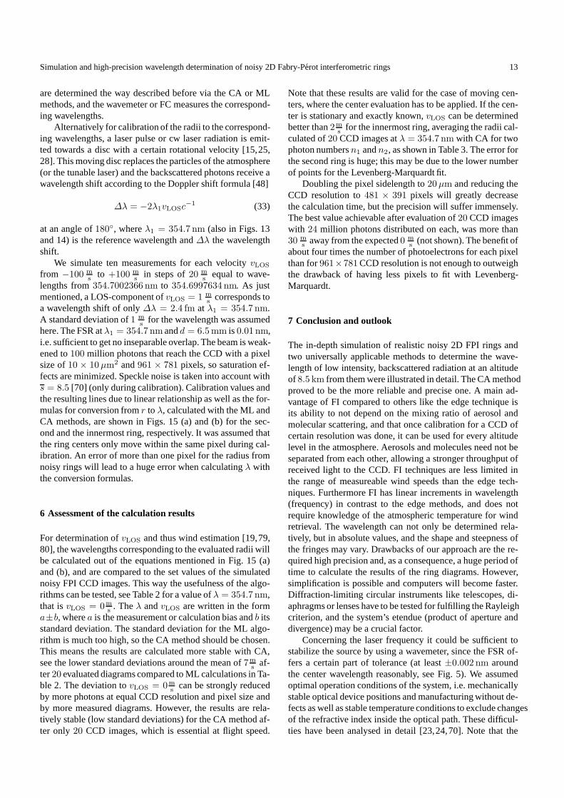
Fig. 15 Calibration lines for the two inner rings ( (a) for the secondring, (b) for the innermost ring; radii calculated via the MLand CAmethods) at tuned wavelengths: the equations include the calculatedrelation between the wavelengths and the radii.

quency combs (FCs) have revolutionized the way and pre-cision the wavelength of light can be measured [77,78] andare a highly suitable source for wavelength determination ofa cw-laser. For calibration a low-power, frequency-tripled,slightly tunable Nd:YAG cw-laser is proposed here. The nearlymonochromatic laser light will generate narrower and steeperrings and peaks on the CCD, thus having less points to fit, butwith less noise, too. The CCD’s resolution is the limiting fac-tor for radii determination and thus calibration. The tunablelaser emits a beam, that is split into two parts: one for the FPIin the mode it will be operating later under fixed plate dis-tance, with the CCD at the end of the light propagation, andthe other for the wavemeter or FC. The CCD diagrams radii


are determined the way described before via the CA or MLmethods, and the wavemeter or FC measures the correspond-ing wavelengths.

Alternatively for calibration of the radii to the correspond-ing wavelengths, a laser pulse or cw laser radiation is emit-ted towards a disc with a certain rotational velocity [15,25,28]. This moving disc replaces the particles of the atmosphere(or the tunable laser) and the backscattered photons receive awavelength shift according to the Doppler shift formula [48]

∆λ = −2λ1vLOSc−1 (33)

at an angle of180, whereλ1 = 354.7 nm (also in Figs. 13and 14) is the reference wavelength and∆λ the wavelengthshift.

We simulate ten measurements for each velocityvLOS

from −100 ms to +100 m

s in steps of20 ms equal to wave-

lengths from354.7002366 nm to 354.6997634 nm. As justmentioned, a LOS-component ofvLOS = 1 m

s corresponds toa wavelength shift of only∆λ = 2.4 fm at λ1 = 354.7 nm.A standard deviation of1 m

s for the wavelength was assumedhere. The FSR atλ1 = 354.7 nmandd = 6.5mm is0.01 nm,i.e. sufficient to get no inseparable overlap. The beam is weak-ened to100 million photons that reach the CCD with a pixelsize of10 × 10µm2 and961 × 781 pixels, so saturation ef-fects are minimized. Speckle noise is taken into account withs = 8.5 [70] (only during calibration). Calibration values andthe resulting lines due to linear relationship as well as thefor-mulas for conversion fromr toλ, calculated with the ML andCA methods, are shown in Figs. 15 (a) and (b) for the sec-ond and the innermost ring, respectively. It was assumed thatthe ring centers only move within the same pixel during cal-ibration. An error of more than one pixel for the radius fromnoisy rings will lead to a huge error when calculatingλ withthe conversion formulas.

6 Assessment of the calculation results

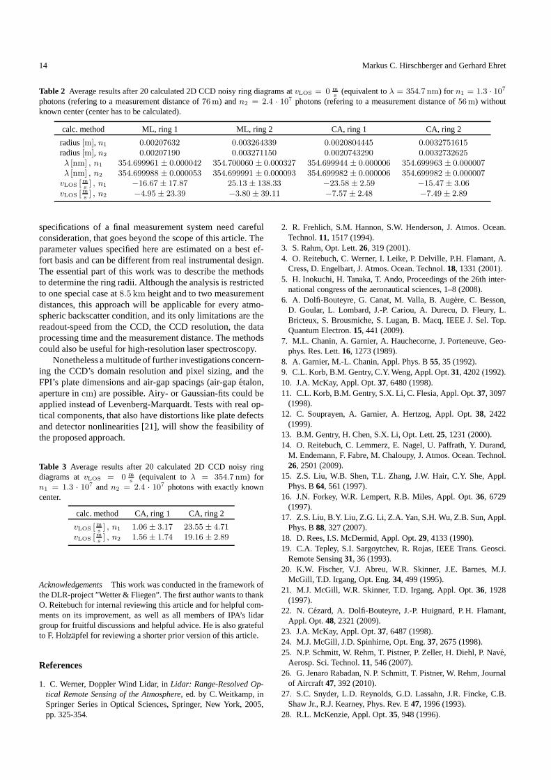
For determination ofvLOS and thus wind estimation [19,79,80], the wavelengths corresponding to the evaluated radii willbe calculated out of the equations mentioned in Fig. 15 (a)and (b), and are compared to the set values of the simulatednoisy FPI CCD images. This way the usefulness of the algo-rithms can be tested, see Table 2 for a value ofλ = 354.7 nm,that isvLOS = 0m

s . Theλ andvLOS are written in the forma±b, wherea is the measurement or calculation bias andb itsstandard deviation. The standard deviation for the ML algo-rithm is much too high, so the CA method should be chosen.This means the results are calculated more stable with CA,see the lower standard deviations around the mean of7m

s af-ter20 evaluated diagrams compared to ML calculations in Ta-ble 2. The deviation tovLOS = 0m

s can be strongly reducedby more photons at equal CCD resolution and pixel size andby more measured diagrams. However, the results are rela-tively stable (low standard deviations) for the CA method af-ter only 20 CCD images, which is essential at flight speed.

Note that these results are valid for the case of moving cen-ters, where the center evaluation has to be applied. If the cen-ter is stationary and exactly known,vLOS can be determinedbetter than2m

s for the innermost ring, averaging the radii cal-culated of20 CCD images atλ = 354.7 nm with CA for twophoton numbersn1 andn2, as shown in Table 3. The error forthe second ring is huge; this may be due to the lower numberof points for the Levenberg-Marquardt fit.

Doubling the pixel sidelength to20µm and reducing theCCD resolution to481 × 391 pixels will greatly decreasethe calculation time, but the precision will suffer immensely.The best value achievable after evaluation of20 CCD imageswith 24 million photons distributed on each, was more than30 m

s away from the expected0 ms (not shown). The benefit of

about four times the number of photoelectrons for each pixelthan for961×781CCD resolution is not enough to outweighthe drawback of having less pixels to fit with Levenberg-Marquardt.

7 Conclusion and outlook

The in-depth simulation of realistic noisy 2D FPI rings andtwo universally applicable methods to determine the wave-length of low intensity, backscattered radiation at an altitudeof 8.5 km from them were illustrated in detail. The CA methodproved to be the more reliable and precise one. A main ad-vantage of FI compared to others like the edge technique isits ability to not depend on the mixing ratio of aerosol andmolecular scattering, and that once calibration for a CCD ofcertain resolution was done, it can be used for every altitudelevel in the atmosphere. Aerosols and molecules need not beseparated from each other, allowing a stronger throughput ofreceived light to the CCD. FI techniques are less limited inthe range of measureable wind speeds than the edge tech-niques. Furthermore FI has linear increments in wavelength(frequency) in contrast to the edge methods, and does notrequire knowledge of the atmospheric temperature for windretrieval. The wavelength can not only be determined rela-tively, but in absolute values, and the shape and steepness ofthe fringes may vary. Drawbacks of our approach are the re-quired high precision and, as a consequence, a huge period oftime to calculate the results of the ring diagrams. However,simplification is possible and computers will become faster.Diffraction-limiting circular instruments like telescopes, di-aphragms or lenses have to be tested for fulfilling the Rayleighcriterion, and the system’s etendue (product of aperture anddivergence) may be a crucial factor.

Concerning the laser frequency it could be sufficient tostabilize the source by using a wavemeter, since the FSR of-fers a certain part of tolerance (at least±0.002 nm aroundthe center wavelength reasonably, see Fig. 5). We assumedoptimal operation conditions of the system, i.e. mechanicallystable optical device positions and manufacturing withoutde-fects as well as stable temperature conditions to exclude changesof the refractive index inside the optical path. These difficul-ties have been analysed in detail [23,24,70]. Note that the


Table 2 Average results after 20 calculated 2D CCD noisy ring diagrams atvLOS = 0 m

s(equivalent toλ = 354.7 nm) for n1 = 1.3 · 107

photons (refering to a measurement distance of76m) andn2 = 2.4 · 107 photons (refering to a measurement distance of56m) withoutknown center (center has to be calculated).

calc. method ML, ring 1 ML, ring 2 CA, ring 1 CA, ring 2

radius[m], n1 0.00207632 0.003264339 0.0020804445 0.0032751615radius[m], n2 0.00207190 0.003271150 0.0020743290 0.0032732625λ [nm] , n1 354.699961 ± 0.000042 354.700060 ± 0.000327 354.699944 ± 0.000006 354.699963 ± 0.000007λ [nm] , n2 354.699988 ± 0.000053 354.699991 ± 0.000093 354.699982 ± 0.000006 354.699982 ± 0.000007

vLOS [m

s] , n1 −16.67 ± 17.87 25.13 ± 138.33 −23.58 ± 2.59 −15.47± 3.06

vLOS [m

s] , n2 −4.95± 23.39 −3.80± 39.11 −7.57 ± 2.48 −7.49± 2.89

specifications of a final measurement system need carefulconsideration, that goes beyond the scope of this article. Theparameter values specified here are estimated on a best ef-fort basis and can be different from real instrumental design.The essential part of this work was to describe the methodsto determine the ring radii. Although the analysis is restrictedto one special case at8.5 km height and to two measurementdistances, this approach will be applicable for every atmo-spheric backscatter condition, and its only limitations are thereadout-speed from the CCD, the CCD resolution, the dataprocessing time and the measurement distance. The methodscould also be useful for high-resolution laser spectroscopy.

Nonetheless a multitude of further investigations concern-ing the CCD’s domain resolution and pixel sizing, and theFPI’s plate dimensions and air-gap spacings (air-gap etalon,aperture incm) are possible. Airy- or Gaussian-fits could beapplied instead of Levenberg-Marquardt. Tests with real op-tical components, that also have distortions like plate defectsand detector nonlinearities [21], will show the feasibility ofthe proposed approach.

Table 3 Average results after 20 calculated 2D CCD noisy ringdiagrams atvLOS = 0 m

s(equivalent toλ = 354.7 nm) for

n1 = 1.3 · 107 andn2 = 2.4 · 107 photons with exactly knowncenter.

calc. method CA, ring 1 CA, ring 2

vLOS [m

s] , n1 1.06± 3.17 23.55 ± 4.71

vLOS [m

s] , n2 1.56± 1.74 19.16 ± 2.89

AcknowledgementsThis work was conducted in the framework ofthe DLR-project ”Wetter & Fliegen”. The first author wants tothankO. Reitebuch for internal reviewing this article and for helpful com-ments on its improvement, as well as all members of IPA’s lidargroup for fruitful discussions and helpful advice. He is also gratefulto F. Holzapfel for reviewing a shorter prior version of this article.

References

1. C. Werner, Doppler Wind Lidar, inLidar: Range-Resolved Op-tical Remote Sensing of the Atmosphere, ed. by C. Weitkamp, inSpringer Series in Optical Sciences, Springer, New York, 2005,pp. 325-354.

2. R. Frehlich, S.M. Hannon, S.W. Henderson, J. Atmos. Ocean.Technol.11, 1517 (1994).

3. S. Rahm, Opt. Lett.26, 319 (2001).4. O. Reitebuch, C. Werner, I. Leike, P. Delville, P.H. Flamant, A.

Cress, D. Engelbart, J. Atmos. Ocean. Technol.18, 1331 (2001).5. H. Inokuchi, H. Tanaka, T. Ando, Proceedings of the 26th inter-

national congress of the aeronautical sciences, 1–8 (2008).6. A. Dolfi-Bouteyre, G. Canat, M. Valla, B. Augere, C. Besson,

D. Goular, L. Lombard, J.-P. Cariou, A. Durecu, D. Fleury, L.Bricteux, S. Brousmiche, S. Lugan, B. Macq, IEEE J. Sel. Top.Quantum Electron.15, 441 (2009).

7. M.L. Chanin, A. Garnier, A. Hauchecorne, J. Porteneuve, Geo-phys. Res. Lett.16, 1273 (1989).

8. A. Garnier, M.-L. Chanin, Appl. Phys. B55, 35 (1992).9. C.L. Korb, B.M. Gentry, C.Y. Weng, Appl. Opt.31, 4202 (1992).10. J.A. McKay, Appl. Opt.37, 6480 (1998).11. C.L. Korb, B.M. Gentry, S.X. Li, C. Flesia, Appl. Opt.37, 3097

(1998).12. C. Souprayen, A. Garnier, A. Hertzog, Appl. Opt.38, 2422

(1999).13. B.M. Gentry, H. Chen, S.X. Li, Opt. Lett.25, 1231 (2000).14. O. Reitebuch, C. Lemmerz, E. Nagel, U. Paffrath, Y. Durand,

M. Endemann, F. Fabre, M. Chaloupy, J. Atmos. Ocean. Technol.26, 2501 (2009).

15. Z.S. Liu, W.B. Shen, T.L. Zhang, J.W. Hair, C.Y. She, Appl.Phys. B64, 561 (1997).

16. J.N. Forkey, W.R. Lempert, R.B. Miles, Appl. Opt.36, 6729(1997).

17. Z.S. Liu, B.Y. Liu, Z.G. Li, Z.A. Yan, S.H. Wu, Z.B. Sun, Appl.Phys. B88, 327 (2007).

18. D. Rees, I.S. McDermid, Appl. Opt.29, 4133 (1990).19. C.A. Tepley, S.I. Sargoytchev, R. Rojas, IEEE Trans. Geosci.

Remote Sensing31, 36 (1993).20. K.W. Fischer, V.J. Abreu, W.R. Skinner, J.E. Barnes, M.J.

McGill, T.D. Irgang, Opt. Eng.34, 499 (1995).21. M.J. McGill, W.R. Skinner, T.D. Irgang, Appl. Opt.36, 1928

(1997).22. N. Cezard, A. Dolfi-Bouteyre, J.-P. Huignard, P. H. Flamant,

Appl. Opt.48, 2321 (2009).23. J.A. McKay, Appl. Opt.37, 6487 (1998).24. M.J. McGill, J.D. Spinhirne, Opt. Eng.37, 2675 (1998).25. N.P. Schmitt, W. Rehm, T. Pistner, P. Zeller, H. Diehl, P.Nave,

Aerosp. Sci. Technol.11, 546 (2007).26. G. Jenaro Rabadan, N. P. Schmitt, T. Pistner, W. Rehm, Journal

of Aircraft 47, 392 (2010).27. S.C. Snyder, L.D. Reynolds, G.D. Lassahn, J.R. Fincke, C.B.

Shaw Jr., R.J. Kearney, Phys. Rev. E47, 1996 (1993).28. R.L. McKenzie, Appl. Opt.35, 948 (1996).


29. R.G. Seasholtz, A.E. Buggele, M.F.Reeder, Opt. Lasers Eng.27, 543 (1997).

30. M.M. Clem, A.F. Mielke-Fagan, K.A. Elam, ”Study of Fabry-Perot Etalon Stability and Tuning for Spectroscopic RayleighScattering,” 48th AIAA Aerospace Sciences Meeting Includingthe New Horizons Forum and Aerospace Exposition, Orlando,Florida, Jan. 4-7, 2010, AIAA 2010-855.

31. T.L. Killeen, B.C. Kennedy, P.B. Hays, D.A. Symanow, D.H.Ceckowski, Appl. Opt.22, 3503 (1983).

32. P.B. Hays, Appl. Opt.29, 1482 (1990).33. J. Wu, J. Wang, P.B. Hays, Appl. Opt.33, 7823 (1994).34. M.J. McGill, M. Marzouk, V.S. Scott, J.D. Spinhirne, Opt. Eng.

36, 2171 (1997).35. J.M. Vaughan,The Fabry-Perot Interferometer(Adam Hilger,

Bristol, 1989).36. G. Hernandez,Fabry-Perot interferometers(Cambridge Uni-

versity Press, 1986).37. K.W. Meissner, J. Opt. Soc. Am.31, 405 (1941).38. N. Barakat, M. Medhat, Optica Acta33, 939 (1986).39. T.J. Scholl, S.J. Rehse, R.A. Holt, S.D. Rosner, Rev. Sci. In-

strum.75, 3318 (2004).40. M. O’Hora, B. Bowe, V. Toal, J. Opt. A: Pure Appl. Opt.7, 364

(2005).41. T. Schroder, C. Lemmerz, O. Reitebuch, M. Wirth, C. Wuhrer,

R. Treichel, Appl. Phys. B87, 437 (2007).42. V.A. Banakh, I.N. Smalikho, F. Kopp, C. Werner, Appl. Opt.

34, 2055 (1995).43. S.R. Pal, A.I. Carswell, Appl. Opt.15, 1990 (1976).44. L.R. Bissonnette, P. Bruscaglioni, A. Ismaelli, G. Zaccanti,

A. Cohen, Y. Benayahu, M. Kleiman, S. Egert, C. Flesia, P.Schwendimann, A.V. Starkov, M. Noormohammadian, U.G. Op-pel, D.M. Winker, E.P. Zege, I.L. Katsev, I.N. Polonsky, Appl.Phys. B60, 355 (1995).

45. L.I. Chaikovskaya, E.P. Zege, I.L. Katsev, M. Hirschberger,U.G. Oppel, Appl. Opt.48, 623 (2009).

46. D. Pierrottet, F. Amzajerdian, L. Petway, B. Barnes, G.Lockard, Proc. SPIE7323, 732311 (2009).

47. N. Lindlein, G. Leuchs, Geometrical Optics, Chap. 2.4 RayTracing, inSpringer Handbook of Lasers and Optics, ed. by F.Trager, Springer, New York, 2007, pp. 61-67.

48. W. Demtroder,Laser Spectroscopy, Vol. 1: Basic Principles(Springer, Berlin Heidelberg, 4th ed. 2008).

49. A. Ansmann, U. Wandinger, O. Le Rille, D. Lajas, A.G.Straume, Appl. Opt.46, 6606 (2007).

50. U. Paffrath, C. Lemmerz, O. Reitebuch, B. Witschas, I. Niko-laus, V. Freudenthaler, J. Atmos. Ocean. Technol.26, 2516 (2009).

51. J.M. Vaughan, D.W. Brown, C. Nash, S.B. Alejandro, G.G.Koenig, J. Geophys. Res.,100(D1), 1043 (1995).

52. J.M. Vaughan, N.J. Geddes, P.H. Flamant, C. Flesia, ”Establish-ment of a backscatter coefficient and atmospheric database,” ESAcontract 12510/97/NL/RE, 110 p. , (1998).

53. A.T. Young, Phys. Today35, 42–48 (January 1982).54. A.T. Young, G.W. Kattawar, Appl. Opt.22, 3668 (1983).55. C.-Y. She, Appl. Opt.404875, (2001).56. R.B. Miles, W.R. Lempert, J.N. Forkey, Meas. Sci. Technol. 12,

R33-R51 (2001).57. B.-Y. Liu, M. Esselborn, M. Wirth, A. Fix, D.-C. Bi, G. Ehret,

Appl. Opt.48, 5143 (2009).58. B. Witschas, M. Vieitez, E.-J. van Duijn, O. Reitebuch, W. van

de Water, W. Ubachs, Appl. Opt.49, 4217 (2010).59. R.T.H. Collis, P.B. Russell, ”Lidar measurement of particles

and gases by elastic backscattering and differential absorption,” in

Laser Monitoring of the Atmosphere, ed. by E.D. Hinkley, Topicsin Applied Physics, Vol.14, Springer, Berlin, Heidelberg, 1976,pp. 71-151.

60. R.M. Measures,Laser Remote Sensing(Wiley, Florida, 1992).61. G.J. Marseille, A. Stoffelen, Q. J. R. Meteorol. Soc.129, 3079

(2003).62. K.S.W. Champion, ”Standard and reference atmospheres,” in

Handbook of geophysics and the space environment, ed. byA.S. Jursa, United States Air Force Geophysics Laboratory,14-1 (1985).

63. G.A. Reider,photonik (Springer, Wien New York, 2nd ed.2005).

64. http://www.pco.de/intensified-cameras/dicam-pro/ ,2010.65. K. Arisaka, Nucl. Instr. and Meth. A442, 80 (2000).66. J.E. Carranza, E. Gibb, B.W. Smith, D.W. Hahn, J.D. Wineford-

ner, Appl. Opt.42, 6016 (2003).67. W.H. Press, S.A. Teukolsky, W.T. Vetterling, B.P. Flannery,Nu-

merical recipes: the art of scientific computing(Cambridge, 3rded., 2007).

68. D. Dussault, P. Hoess, Proc. SPIE,5563, 195 (2004).69. Z. Liu, W. Hunt, M. Vaughan, C. Hostetler, M. McGill, K. Pow-

ell, D. Winker, Y. Hu, Appl. Opt.45, 4437 (2006).70. N. Cezard, A. Dolfi-Bouteyre, J.-P. Huignard, P. Flamant, Proc.

of SPIE,6750, 0801-0810 (2007).71. G. Ehret, C. Kiemle, M. Wirth, A. Amediek, A. Fix, S. Houwel-

ing, Appl. Phys. B90, 593 (2008).72. B. Mayer, A. Kylling, Atmos. Chem. Phys. Discuss.,5, 1319

(2005).73. C. Flesia, C.L. Korb, Appl. Opt.38, 432 (1999).74. J.E. Bresenham, IBM Systems Journal4, 25 (1965).75. A. Savitzky, M.L.E. Golay, Anal. Chem.36, 1627 (1964).76. H. Ziegler, Appl. Spectrosc.35, 88 (1981).77. S.A. Diddams, D.J. Jones, J. Ye, S.T. Cundiff, J.L. Hall,J.K.

Ranka, R.S. Windeler, R. Holzwarth, Th. Udem, T.W. Hansch,Phys. Rev. Lett.84, 5102 (2000).

78. Th. Udem, R. Holzwarth, T.W. Hansch, Nature416, 233 (2002).79. R. Frehlich, J. Atmos. Oceanic Technol.18, 1628 (2001).80. F. Andreucci, M.V. Arbolino, IEEE Geoscience & remote sens-

ing Symposium, 1995, Vol. 3, pp. 2319–2322.

Documents

Simulation and high-precision wavelength determination of